July/August/September 2011

Vol 26 No 3

Spotlight on SEM for economists

(and others who think they don’t care)This article is for those who are unfamiliar with SEM, who do not see publications using SEM in their field, or who otherwise think they don’t care about SEM.

p. 4 The Stata News: Executive Editor: ........... Karen Strope

Production Supervisor: ... Annette Fett

New public training courses and datesIntensive, in-depth courses taught by StataCorp around the country.

p. 6

Have you upgraded yet?Stata 12 is now shipping. If you haven’t upgraded, you are missing exciting new statistics and a host of new features.

• SEM (structural equation modeling)

• Chained equations in MI

• Survey support for mixed models

• Contour plots

• Contrasts

• Pairwise comparisons

• ARFIMA

• Multivariate GARCH

• UCM (unobserved components model)

• Time-series filters

• Business calendars

• Margins plots

• ROC analysis

• Automatic memory management

• Excel import/export

• Installation Qualification

• More ...

m1

m2

m3

m4

m5

m6

m7

L1

L2

L3

ε1

ε2

ε3

ε4

ε8ε5

ε6

ε7

65,0

0075

,000

85,0

00N

orth

ing

30,000 35,000 40,000 45,000 49,000Easting

7,600

7,700

7,800

7,900

8,000

Dep

th (f

t)

Subsea elevation of Lamont Sandstone, Ohio

46

810

1214

1970m1 1980m1 1990m1 2000m1 2010m1Month

median duration of unemployment trend, smooth

−2−1

01

2se

ason

al, s

moo

th

1970m1 1980m1 1990m1 2000m1 2010m1Month

95% CI

−.4

−.3

−.2

−.1

0.1

10 20 30 40 50 60Body Mass Index (BMI)

Male−Female Contrasts of Predictive Margins of Pr(HighBP)

Upgrade today! www.stata.com

RELEASE

SEM (structural equation modeling)

SEM has something for nearly

every researcher in nearly every

discipline.

Those of you who have been

asking for SEM know why you

want it: confirmatory factor

analysis, measurement-error

models, path analysis models,

multiple-factor measurement models, MIMIC models, latent growth models,

correlated uniqueness models, standardized and unstandardized estimates,

modification indices.

If you are not familiar with SEM, you should consider that it can elegantly

handle endogenous variables, confounding variables, mediating variables,

moderated effects, observed and latent variables, univariate outcomes,

and multivariate outcomes. Aside from standard linear models such as

regression, multivariate regression, and seemingly unrelated regression,

here are some of the models you can fit with sem: simultaneous systems

with all observed variables or with observed and latent variables; random-

effects models with latent (unobserved) dependent variables or with

endogenous variables; random-effects models with autocorrelated errors;

or any combination of the preceding. In all cases, sem can easily estimate

direct, indirect, and total effects of covariates.

SEM is a framework that encompasses most univariate and multivariate

linear models and also provides for latent (unobserved) variables and for

dependent variables that simultaneously affect each other. It also supports

correlations of errors, including autocorrelation in panel data.

Stata 12’s new sem command provides an intuitive syntax for specifying

models. sem y <- x1 x2 x3

specifies a linear regression model of y on x1, x2, and x3. We might also

say it creates three paths, one from each x to y.

sem (x1 -> y) (x2 -> y) (x3 -> y)

is an equivalent specification.

sem y1 y2 <- x1 x2 x3

specifies a multivariate regression of y1 and y2 on x1, x2, and x3.

sem (y1 <- y2 x1) (y2 <- y1 x2)

specifies a simultaneous system where the dependent variables y1 and y2

are affected by each other.

sem L -> m1 m2 m3

specifies a measurement model where the latent variable L is measured by

the observed measurement variables m1, m2, and m3.

All the above may be combined in sem to create complex structural models.

If you prefer to build models graphically, the SEM Builder is integrated into

Stata 12 and provides all the tools you need to graphically create and

estimate SEMs.

Missing data: Chained equations (and more) in MI

New features in Stata 12’s MI (multiple imputation) facilities dramatically

expand your options in handling missing data.

Chained equations let you handle arbitrary missing-data patterns

in continuous, ordinal, cardinal, and count variables. This method is

also known as sequential regression multivariate imputation (SRMI).

It supports imputation via linear, truncated, interval censored, logit/

logistic, ordered logit, multinomial logit, Poisson, and negative

binomial regressions.

Conditional imputation lets you customize imputation within

groups, even when the group identifier itself is missing.

Simulation error can now be estimated.

Panel and multilevel data are now supported.

Predictions, both linear and nonlinear, can now be performed.

Contrasts and pairwise comparisons

The new contrast command makes it simple to compare and

contrast the effects of categorical and indicator covariates, whether the

estimator is ANOVA, linear regression, logistic regression, or virtually any

of Stata’s 140 estimators. Named contrasts let you automatically compare

against reference categories, adjacent categories, the grand mean, or all

prior categories. It can also perform orthogonal polynomial contrasts and

handle multiway interactions.

Beyond the named contrasts, you can create any custom contrast. The

interaction operator works with custom contrasts, saving you the tedium

of creating tables that perform inner products of multiway contrasts.

contrast also performs ANOVA-style tests of main effects, interaction

effects, simple effects, and nested effects after any estimator.

Moreover, the margins command now supports contrast operators so

that contrasts can be obtained for any results from margins—from

estimated marginal means and conditional probabilities to marginal effects

and population-averaged probabilities.

The new pwmean command performs all pairwise comparisons of the

means across groups or interactions of multiple groups.

The new pwcompare command performs pairwise comparisons of

estimated means and estimated marginal means after fitting a model with

almost any estimator.

Pairwise comparisons of nonlinear responses and their margins are now

supported by the margins command.

The contrast, pwmean, pwcompare, and margins

commands all provide adjustments for multiple comparisons using

Bonferroni, Šidák, Scheffé, Tukey, SNK, Duncan, and Dunnett methods.

2

Margins plotsGraph anything that margins can compute—

estimated means, marginal probabilities,

conditional or population-averaged effects,

marginal effects, contrasts, and more. Graph within

or across one or more groups or factor-variable levels. Easily!

Survey-data support for multilevel mixed modelsLinear mixed models estimated via xtmixed now support sampling weights; robust and cluster-

robust standard errors; and, for survey data, standard errors adjusted for the first level of sampling

(primary sampling units, PSUs).

Time-series: Multivariate GARCH, ARFIMA, UCM, filtersStata 12 has a phalanx of new time-series estimators and filters.

A full suite of multivariate GARCH models joins the diagonal vech estimator

that was previously available. Advanced conditional correlation structures are

now supported with the CCC (constant conditional correlation), DCC (dynamic

conditional correlation), and VCC (varying conditional correlation) estimators.

In- and out-of-sample predictions of the conditional variance are available

after all models.

ARFIMA (autoregressive fractionally integrated moving average) is now

available to estimate long-memory processes that reside in the middle

ground between short-memory (ARMA) process and fully integrated (ARIMA) models.

Stata 12 has time-series filters to decompose a series into trend and cyclic components. Four filters are

available: the Baxter–King and Christiano–Fitzgerald band-pass filters, and the Butterworth and Hodrick–

Prescott high-pass filters.

The new UCM (unobserved components model) estimator provides a flexible, modern, and formal

framework for decomposing a series into trend, seasonal, cyclic, and idiosyncratic components. A

major advantage of the UCM framework is the ease of interpretation and the direct relevance of the

trend, cyclic, and spectral components.

Business datesStata 12 handles business dates—dates that exclude Saturday and Sunday.

What’s more, you can define your own business dates using business calendars. Create dates for the

New York, London, Tokyo, Shanghai, Deutsche Börse, or other stock exchanges. Or, create a calendar

for your own institution.

ROC analysisStata 12 can model ROC curves that control for covariates. Think of it as

regression for ROC. It can also test whether ROC curves differ or the areas

under the curve (AUC) differ across groups, adjusting for covariates.

Excel import/exportStata 12 can now directly import data from and export data to Microsoft Excel files.

On Windows, Mac, or Linux, you can import any worksheet or partial worksheet from multisheet workbooks.

You can export Stata data to create a new workbook, replace or add a worksheet in an existing workbook, or

modify a subset of cells. Stata variable and value labels are supported, as is automatic conversion of dates.

Automatic memory managementYou no longer have to tell Stata how much

memory to use.

Stata 12 automatically adjusts its memory

according to the size of your dataset, even as

you create new variables or merge and append

datasets.

As a side benefit, Stata 12 often can access

more of the memory available on 32-bit

Windows computers.

Interface enhancementsThe Stata 12 window is laid out

to better take advantage of wide

computer monitors. Better yet,

you can manage your variables—including the

labels, value labels, notes, formats, and types—

directly from the new Properties window on the

main Stata 12 interface. You can do the same

in the Data Editor. You can also now filter your

commands and variables to show only what

you are interested in. The new version of the

Viewer is tabbed and has direct links to dialog

boxes, also sees, and sections of the help files

(Options, Examples, etc.).

Contour plots

And moreThere are too many new features to list here.

We have not discussed spectral density plots,

functions for Tukey’s Studentized range and

Dunnett’s multiple range, or new estimators for

truncated count-data regressions.

www.stata.com/stata12

−15

−10

−5

0

5

20−29 30−39 40−49 50−59 60−69 70+Age Group

Contrasts by Sex of Estimated Means by Age Group

95% CI

−.4

−.3

−.2

−.1

0.1

10 20 30 40 50 60Body Mass Index (BMI)

Male−Female Contrasts of Predictive Margins of Pr(HighBP)

110

120

130

140

150

20−29 30−39 40−49 50−59 60−69 70+Age Group

MaleFemale

Estimated Means by Age Group and Sex with 95% CIs

−0.25

−0.125

0

0.125

0.25

1920 1930 1940 1950 1960 1970 1980 1990 2000 2010Quarterly data

Recessions highlightedButterworth Cyclical Component

00.

001

0.00

20.

003

01jan2009 01jul2009 01jan2010 01jul2010 01jan2011 01jul2011

ToyotaNissanHonda

Modeled & Forecast Variances of Stock Returns

0

0.25

0.5

0.75

1

True

-pos

itive

rate

(RO

C)

0 0.25 0.5 0.75 1False-positive rate

reference30 mos.40 mos.50 mos.

ROC, by age

02

46

Nor

th−S

outh

(50−

ft)

0 2 4 6East−West (50−ft)

925900875850825800775750725700

Elevation of Rock Formation

65,0

0075

,000

85,0

00N

orth

ing

30,000 35,000 40,000 45,000 49,000Easting

7,600

7,700

7,800

7,900

8,000

Dep

th (f

t)

Subsea elevation of Lamont Sandstone, Ohio

3

Spotlight on SEM for economists (and others who think they don’t care)

This article is not for those who know about SEM (structural equation

modeling). Those who want measurement models, path analysis,

confirmatory factor analysis, MIMIC models, latent growth models, and

general structural relations among unobserved (latent) regressors and

outcomes. Those who want all the above with simple and elegant handling

of missing data. This article is for those who are unfamiliar with SEM, who

do not see publications using SEM in their field, or who otherwise think they

don’t care about SEM.

I am not going to try to convince you that you want the things listed above

(though there are likely some useful tools in that list for you). Rather, I am

going to show you some cases where SEM can fit models that you know

and use, and can fit them in more flexible ways and with extensions not

available with your usual estimators.

Extensions to SUR

Let’s start with seemingly unrelated regression (SUR), which is just an

extension of multivariate regression wherein each dependent variable can

depend on a different set of covariates, making the coefficient estimates

themselves depend on the covariance of the disturbances and not just their

standard errors. A simple three-equation model is

y1 = β

1 x

1 + β

2 x

2 + ε

1 ε

1 ~ i.i.d. normal(0, σ

12)

y2 = β

3 x

1 + β

4 x

3 + ε

2 ε

2 ~ i.i.d. normal(0, σ

22)

y3 = β

5 x

1 + β

6 x

2 + β

7 x

3 + ε

3 ε

3 ~ i.i.d. normal(0, σ

32)

and ε1, ε

2, and ε

3 are correlated.

Note that the normality assumption is not required for asymptotic

inference.

We typically estimate such models in Stata by the method of generalized

least squares (GLS) using sureg: sureg (y1 x1 x2) (y2 x1 x3) (y3 x1 x2 x3)

In Stata 12, we can estimate that same model by maximum likelihood (ML)

using sem: sem (y1 <- x1 x2) (y2 <- x1 x3) (y3 <- x1 x2 x3), covstruct(e.oendogenous, unstructured)

One nice thing about the ML estimates is that their standard errors (SEs) do

not assume we have perfectly estimated the correlations among the errors.

Rather, those correlations are simply more free parameter estimates in the

model.

Nicer still are the extensions we get from sem.

We can apply any constraints we wish to the covariance matrix of the

errors. For example, sem (y1 <- x1 x2) (y2 <- x1 x3) (y3 <- x1 x2 x3), covstruct(e.oendogenous, exchangeable)

makes all the ε’s homoskedastic (σ1 = σ2 = σ3 ) and with a single shared

correlation. sem supports several other identified covariance structures,

or you can supply a covariance pattern, a fixed covariance matrix, or apply

individual constraints to the variances and covariance of the ε’s.

We can obtain SEs, confidence intervals (CIs), and associated tests that are

robust to lack of independence within identified groups of observations: sem (y1 <- x1 x2) (y2 <- x1 x3) (y3 <- x1 x2 x3), vce(cluster group)

And, we can do any of the above when the data are “unbalanced”—that is,

when there is a different number of “observations” for y1, y2, or y3, sem (y1 <- x1 x2) (y2 <- x1 x3) (y3 <- x1 x2 x3), method(mlmv)

Put another way, values of y1, y2, and y3 can be missing at random

(MAR), and we can still use the information on the other variables. The

MAR assumption, also called “selection on observables”, stipulates that the

missingness depends only on the values of y1, y2, y3, x1, x2, and x3 and

does not depend on variables that are not observed.

When only the y ’s are missing, the mlmv estimation method adds no

additional assumptions to the estimation. We can also estimate using mlmv

when there are missing values in the x’s, but we must then make the much

more binding assumption that the x’s are distributed multivariate normal.

Endogeneity

Endogeneity simply means that there is a correlation between a regressor

and the error term in a regression. Endogeneity presents a fundamental

problem for parameter estimation. If the endogeneity is not accounted

for, then the parameter estimates will be biased and inconsistent—no

amount of data is going to make the estimates less biased. Endogeneity

arises in a number of situations: simultaneous systems, omitted variables/

confounders, measurement error, correlated disturbances, and others. All

these problems can be addressed with SEM. The approach is most direct

for simultaneous systems.

Simultaneous systems arise when two or more dependent variables affect

each other.

y1 = β

1 y

2 + β

2 x

1 + β

3 x

2 + ε

1

y2 = β

4 y

1 + β

5 x

1 + β

6 x

3 + ε

2

We often make assumptions about the ε’s being normally distributed

and correlated, though many estimators are robust to these

assumptions.

The endogeneity is obvious: a function of y1, y

2 is clearly correlated with

y1’s disturbance. Why not just estimate the reduced-form equations that

result from substituting the expression for y1 into the equation for y

2 and

vice versa? The structure of our original equations often arises from theory,

and the parameters in the equations are themselves of primary interest. A

classic example in economics would have y1 be the quantity demanded

of a product and y2 be the price of the product. β

1 is clearly an important

parameter, relating the quantity demanded to the offering price.

4

Such parameters are so important that economists have a name for

them—structural parameters—and the equations are so important that

we have a name for them—structural equations. It is the height of irony

that you rarely, if ever, see the structural equations estimated by structural

equation modeling (SEM), even though “structural” means the same thing

in both parlances. Perhaps we are put off by the latent variables that

can also appear in SEM, though that seems ironic too given the current

popularity of dynamic-factor models (many of which can be estimated by

Stata’s dfactor command).

In Stata 11, you can estimate the above system with the method of three-

stage least squares (3SLS) by typing reg3 (y1 y2 x1 x2) (y2 y1 x1 x3)

In Stata 12, you can also estimate the system with the method of full-

information maximum likelihood (FIML) by typing sem (y1 <- y2 x1 x2) (y2 <- y1 x1 x3), cov(e.y1*e.y2)

For any true SEMers still reading, the path diagram for this model looks like

Like the ML estimator for SUR, the FIML estimator is not conditional on the

estimated covariance of the errors (the 3SLS estimator is).

Also like the ML estimator for SUR, we get some handy extensions not

available in reg3:

• We can control and constrain the structure of the error covariance

matrix.

• We can obtain SEs, CIs, and associated tests that are robust to lack

of independence within identified groups of observations—option

vce(cluster <group>).

• We can handle missing data in the dependent variables, so long as it

is missing on observables.

We can also estimate via GMM (generalized method of moments),

an estimator that makes fewer distributional assumptions—option

method(adf). ADF stands for asymptotic distribution free and is

SEM-speak for GMM.

While the structural parameters (direct effects) are often of primary interest,

we sometimes also want to know the indirect effect of a variable (its effect

through other variables) or its total effect (the direct plus indirect effects).

After estimation with sem, those effects, their SEs, and their CIs are a

command away—estat teffects.

To the right is what

those results might

look like after fitting our

notional model.

sem can also estimate

our simultaneous

system by limited-

information maximum

likelihood (LIML). This

estimator requires that

we know the form

of only the structural

equation of interest,

and we handle the

remaining endogenous

variables using their

reduced forms. We

could also consider

this estimation by

instrumental variables.

For our current model,

in Stata 11 we type

ivregress liml y1 x1 x2 (y2 = x1 x2 x3)

In Stata 12, we can also type sem (y1 <- y2 x1 x2) (y2 <- x1 x2 x3), cov(e.y1*e.y2)

This will estimate the structural model for y1 but only a reduced-form model

for y2. The approach is appropriate for many forms of endogeneity beyond

simultaneous systems. As with SUR and simultaneous systems, sem

offers some flexibility that ivregress does not.

What else?

In all the models considered above, the exogenous or endogenous

variables can represent latent unobservable quantities or quantities that

are measured with error. But here we enter the true realm of SEM and I

promised not to go there.

How about that, with a little effort, sem can extend all the models above

into random-effects panel-data models or even multilevel random-effects

models. Once in SEM form, other extensions also suggest themselves—

correlations across the groups in a level (not possible in either xtmixed

or xtreg), making the random effects conditional, and more. For an

overview of this approach, see the Not Elsewhere Classified blog posting at

www.stata.com/blog/xtsem.

If you have been dismissing SEM as “not for you”, you might want to take

another look.

— Vince Wiggins, Vice President of Scientific Development, StataCorp

5

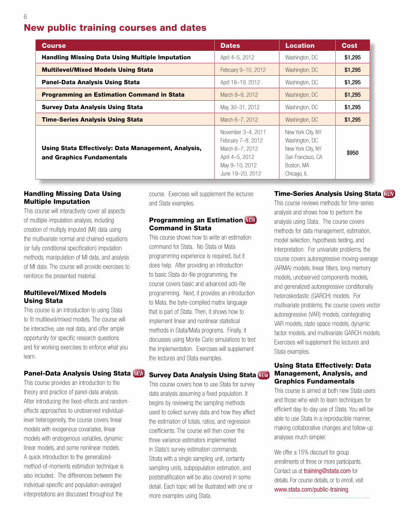
New public training courses and dates

Handling Missing Data Using Multiple ImputationThis course will interactively cover all aspects

of multiple-imputation analysis, including

creation of multiply imputed (MI) data using

the multivariate normal and chained-equations

(or fully conditional specification) imputation

methods, manipulation of MI data, and analysis

of MI data. The course will provide exercises to

reinforce the presented material.

Multilevel/Mixed Models Using StataThis course is an introduction to using Stata

to fit multilevel/mixed models. The course will

be interactive, use real data, and offer ample

opportunity for specific research questions

and for working exercises to enforce what you

learn.

Panel-Data Analysis Using StataThis course provides an introduction to the

theory and practice of panel-data analysis.

After introducing the fixed-effects and random-

effects approaches to unobserved individual-

level heterogeneity, the course covers linear

models with exogenous covariates, linear

models with endogenous variables, dynamic

linear models, and some nonlinear models.

A quick introduction to the generalized-

method-of-moments estimation technique is

also included. The differences between the

individual-specific and population-averaged

interpretations are discussed throughout the

course. Exercises will supplement the lectures

and Stata examples.

Programming an Estimation Command in StataThis course shows how to write an estimation

command for Stata. No Stata or Mata

programming experience is required, but it

does help. After providing an introduction

to basic Stata do-file programming, the

course covers basic and advanced ado-file

programming. Next, it provides an introduction

to Mata, the byte-compiled matrix language

that is part of Stata. Then, it shows how to

implement linear and nonlinear statistical

methods in Stata/Mata programs. Finally, it

discusses using Monte Carlo simulations to test

the implementation. Exercises will supplement

the lectures and Stata examples.

Survey Data Analysis Using StataThis course covers how to use Stata for survey

data analysis assuming a fixed population. It

begins by reviewing the sampling methods

used to collect survey data and how they affect

the estimation of totals, ratios, and regression

coefficients. The course will then cover the

three variance estimators implemented

in Stata’s survey estimation commands.

Strata with a single sampling unit, certainty

sampling units, subpopulation estimation, and

poststratification will be also covered in some

detail. Each topic will be illustrated with one or

more examples using Stata.

Time-Series Analysis Using StataThis course reviews methods for time-series

analysis and shows how to perform the

analysis using Stata. The course covers

methods for data management, estimation,

model selection, hypothesis testing, and

interpretation. For univariate problems, the

course covers autoregressive moving-average

(ARMA) models, linear filters, long-memory

models, unobserved components models,

and generalized autoregressive conditionally

heteroskedastic (GARCH) models. For

multivariate problems, the course covers vector

autoregressive (VAR) models, cointegrating

VAR models, state-space models, dynamic

factor models, and multivariate GARCH models.

Exercises will supplement the lectures and

Stata examples.

Using Stata Effectively: Data Management, Analysis, and Graphics FundamentalsThis course is aimed at both new Stata users

and those who wish to learn techniques for

efficient day-to-day use of Stata. You will be

able to use Stata in a reproducible manner,

making collaborative changes and follow-up

analyses much simpler.

We offer a 15% discount for group

enrollments of three or more participants.

Contact us at training@stata.com for

details. For course details, or to enroll, visit

www.stata.com/public-training.

Course Dates Location Cost

Handling Missing Data Using Multiple Imputation April 4–5, 2012 Washington, DC $1,295

Multilevel/Mixed Models Using Stata February 9–10, 2012 Washington, DC $1,295

Panel-Data Analysis Using Stata April 18–19, 2012 Washington, DC $1,295

Programming an Estimation Command in Stata March 8–9, 2012 Washington, DC $1,295

Survey Data Analysis Using Stata May 30–31, 2012 Washington, DC $1,295

Time-Series Analysis Using Stata March 6–7, 2012 Washington, DC $1,295

Using Stata Effectively: Data Management, Analysis,

and Graphics Fundamentals

November 3–4, 2011

February 7–8, 2012

March 6–7, 2012

April 4–5, 2012

May 9–10, 2012

June 19–20, 2012

New York City, NY

Washington, DC

New York City, NY

San Francisco, CA

Boston, MA

Chicago, IL

$950

NEW

NEW

NEW

NEW

6

New from the Stata Bookstore

Practical Multivariate Analysis, Fifth Edition

Authors: Abdelmonem Afifi, Susanne May,

and Virginia A. Clark

Publisher: Chapman & Hall/CRC

Copyright: 2011

ISBN-13: 978-1-4398-1680-6

Pages: 517; hardcover

Price: $78.50

The fifth edition of Practical Multivariate Analysis, by Afifi, May, and Clark,

provides an applied introduction to the analysis of multivariate data. The

preface says:

“We wrote this book for investigators, specifically behavioral scientists,

biomedical scientists, and industrial or academic researchers, who

wish to perform multivariate statistical analyses and understand the

results. We expect readers to be able to perform and understand the

results, but also expect them to know when to ask for help from an

expert on the subject. It can either be used as a self-guided textbook

or as a text in an applied course in multivariate analysis.”

Sections 1 and 2, the first half of the book, review the basics:

understanding the different types of data, preparing your data, selecting

appropriate statistical techniques, and using and understanding regression

and correlation techniques.

Section 3, the second half of the book, covers canonical correlation,

discriminant analysis, logistic regression, survival analysis, principal

components, factor analysis, cluster analysis, log-linear analysis, and

correlated outcomes regression (think xtmixed in Stata).

The applied introductory nature of the book can be seen in the table of

contents. Most chapters include subsections titled “Chapter outline”, “When

is [this technique] used”, “Data example”, “Basic concepts”, “Discussion of

computer programs”, “What to watch out for”, “Summary”, and “Problems”.

The UCLA website,

www.ats.ucla.edu/stat/examples/cama4

is another resource for readers of this book. Here many of the examples

that were in the fourth edition of the book are demonstrated in Stata and in

four other statistical packages.

The data for the fifth edition are available for download from within Stata so

that you can practice applying the techniques as you read.

If you are looking for derivations and proofs, this book is not for you. If you

are looking for guidance on techniques to use, when to use them, and how

to interpret what they produce, this book will prove helpful.

You can find the table of contents and online ordering information at

www.stata.com/bookstore/practical-multivariate-analysis.

Negative Binomial Regression, Second Edition

Author: Joseph M. Hilbe

Publisher: Cambridge University Press

Copyright: 2011

ISBN-13: 978-0-521-19815-8

Pages: 553; hardcover

Price: $66.50

Negative Binomial Regression, Second Edition, by Joseph M. Hilbe,

reviews the negative binomial model and its variations. Negative binomial

regression—a recently popular alternative to Poisson regression—is used

to account for overdispersion, which is often encountered in many real-

world applications with count responses.

Negative Binomial Regression covers the count response models, their

estimation methods, and the algorithms used to fit these models. Hilbe

details the problem of overdispersion and ways to handle it. The book

emphasizes the application of negative binomial models to various research

problems involving overdispersed count data. Much of the book is devoted

to discussing model-selection techniques, the interpretation of results,

regression diagnostics, and methods of assessing goodness of fit.

Hilbe uses Stata extensively throughout the book to display examples. He

describes various extensions of the negative binomial model—those that

handle excess zeros, censored and truncated data, panel and longitudinal

data, and data from sample selection.

Negative Binomial Regression is aimed at those statisticians,

econometricians, and practicing researchers analyzing count-response

data. The book is written for a reader with a general background in

maximum likelihood estimation and generalized linear models, but Hilbe

includes enough mathematical details to satisfy the more theoretically

minded reader.

This second edition includes added material on finite-mixture models;

quantile-count models; bivariate negative binomial models; and various

methods of handling endogeneity, including the generalized method of

moments.

You can find the table of contents and online ordering information at

www.stata.com/bookstore/negative-binomial-regression.

7

Contact us979-696-4600 979-696-4601 (fax)

service@stata.com www.stata.comPlease include your Stata serial number with all correspondence.

Find a Stata distributor near you www.stata.com/worldwide

Copyright 2011 by StataCorp LP.

Find us on Facebook. Follow us on Twitter. Check out our blog.

StataCorp

4905 Lakeway Drive

College Station, TX 77845

USA

Return service requested.

Serious software for serious researchers. Stata is a registered trademark of StataCorp LP. Serious software for serious researchers is a trademark of StataCorp LP.

Upcoming Stata Users Group meetings

Sweden

The meeting, organized jointly by Metrika Consulting,

Stata’s distributor in the Nordic and Baltic regions, and

Karolinska Institutet is open to everyone. Personnel

from StataCorp will attend, and there will be the

usual “Wishes and grumbles” session at which you

may air your thoughts to Stata developers. Attending

from StataCorp are Yulia Marchenko, Associate

Director, Biostatistics and Vince Wiggins, Vice

President, Scientific Development. For details, visit

www.stata.com/meeting/sweden11.

Italy

The meeting, organized by TStat, Stata’s distributor in

Italy, provides Stata users working in different research

areas with a unique opportunity to exchange ideas,

experiences, and information on user-written routines

and applications. Stata users interested in contributing

to the meeting are encouraged to submit their proposals to the scientific committee. As in previous

years, the emphasis will be on the development of new commands or procedures currently unavailable

in Stata. For details, including a preliminary program, visit www.stata.com/meeting/italy11.

Visit us at APHA 2011

Washington, DC, October 29–November 2

The American Public Heath Association

will have its annual meeting in Washington,

DC from October 29 through November

2. For more information, go to

www.apha.org/meetings/highlights.

Stata representatives, including Bill Rising,

Director of Educational Services, and Theresa

Boswell, Biostatistician and Software Developer,

will be available at the Stata booth to answer

your questions about all things Stata. Stop

by booth #4001 to visit with the people who

develop and support the software and to get

20% off your purchase of Stata Press books

and Stata Journal subscriptions.