July 2006 RFF DP 06-36 DISCUSSION PAPER · July 2006 RFF DP 06-36 Taking up the Slack: Lessons from...
39
1616 P St. NW Washington, DC 20036 202-328-5000 www.rff.org July 2006 RFF DP 06-3 6 Taking up the Slack: Lessons from a Cap- and-Trade Program in Chicago David A. Evans and Joseph A. Kruger DISCUSSION PAPER
Transcript of July 2006 RFF DP 06-36 DISCUSSION PAPER · July 2006 RFF DP 06-36 Taking up the Slack: Lessons from...
1616 P St. NW Washington, DC 20036 202-328-5000 www.rff.org
July 2006 RFF DP 06-36
Taking up the Slack: Lessons from a Cap-and-Trade Program in Chicago
Dav id A . Evans and Joseph A . Krug er
DIS
CU
SSIO
N P
APE
R

© 2006 Resources for the Future. All rights reserved. No portion of this paper may be reproduced without permission of the authors.
Discussion papers are research materials circulated by their authors for purposes of information and discussion. They have not necessarily undergone formal peer review.
Taking Up the Slack
Lessons from a Cap-andTrade Program in Chicago
David A. Evans and Joseph A. Kruger
Abstract The Emissions Reduction Market System (ERMS), an emissions-trading program for volatile
organic materials (VOMs) in Chicago, Illinois, has been characterized by emissions significantly below the annual allocation of emission allowances, allowance prices much lower than predicted, limited trading, and emission allowances that expire unused. Essentially, it appears that a fundamental prerequisite for a tradable allowance program is missing—there is no scarcity of allowances. We evaluate a variety of hypotheses that may explain why the ERMS cap does not appear to be affecting abatement behavior and identify three that contributed to the lack of scarcity in the ERMS program: (1) a baseline process that inflated the cap; (2) hazardous air pollutant regulations that contributed to VOM reductions at some sources; and (3) numerous facility shutdowns. We conclude that the ERMS experience illustrates the inherent unpredictability of economic, regulatory, and other factors when setting an emissions target; a conclusion that resonates with the recent experience of the European Union Emissions Trading Scheme. This argues for gathering reliable emissions data, developing sophisticated emissions projections, and making transparent assumptions about the impacts of other policies and regulations during the program planning and design phase. However, even with all these attributes, it is still difficult to anticipate every possible outcome. Thus, it is desirable to have robust mechanisms to address the uncertainties of emissions-trading markets and to make midcourse corrections if necessary. Finally, we offer some comments on how to think about the results of ERMS versus a hypothetical command and control program that might have been designed to reach the same environmental outcome.
Key Words: emissions-trading, ERMS, European Union, climate change
JEL Classification Numbers: Q53, Q58
Contents
1. Introduction......................................................................................................................... 5
2. Background on ERMS........................................................................................................ 8
2.1 Regulatory Context of Policy Development ................................................................. 8
2.2 Key Features of ERMS ................................................................................................. 9 2.2.1 Affected Sources...................................................................................................9 2.2.2 Allocation of Emission Allowances....................................................................10 2.2.3 Trading and Banking Rules ................................................................................10 2.2.4 Compliance and Enforcement.............................................................................11
2.3 Performance of ERMS................................................................................................ 11
3. Explaining Slackness in the ERMS Cap ......................................................................... 12
3.1 Hypothesis #1: Inflation of Baseline........................................................................... 12
3.2 Hypothesis #2: Other Regulations .............................................................................. 16
3.3 Hypothesis #3: Industry Contraction .......................................................................... 20
3.4 Hypothesis #4: Market Behavior and Uncertainty...................................................... 23
3.5 Hypothesis #5: Innovation and Managerial Empowerment........................................ 25
4. Conclusions/Additional Program Experience/Lessons.................................................. 26
Mechanism to Address Unexpected Outcomes ................................................................ 27
Was the ERMS Program a Success?................................................................................. 29
References.............................................................................................................................. 36
Acronyms
ACMA............Alternative Compliance Market Account
ATU ...............Allotment Trading Unit
CAAA ............Clean Air Act Amendments
CAAPP...........Clean Air Act Permit Program
ERG................Emissions Reduction Generators
ERMS.............Emissions Reduction Market System
EU ETS ..........European Union Emissions Trading Scheme
HAP................hazardous air pollutant
IEPA...............Illinois Environmental Protection Agency
NESHAP........National Emission Standards for Hazardous Air Pollutants
NOX................nitrogen oxide
RECLAIM......Regional Clean Air Incentives Market
ROP................rate-of-progress plan
SIC .................Standard Industrial Classification
TRI .................Toxics Release Inventory
SO2 .................sulfur dioxide
U.S.EPA.........U.S. Environmental Protection Agency
VOMs.............volatile organic materials
Resources for the Future Evans and Krueger
5
Taking up the Slack Cap: Lessons from a Cap-and-Trade Program in Chicago
David A. Evans and Joseph A. Kruger ∗
1. Introduction
Although there is a substantial literature on the U.S. sulfur dioxide (SO2) and nitrogen oxide (NOX) programs1, little attention has been paid a smaller, less publicized cap-and-trade program: the Emissions Reduction Market System (ERMS) for volatile organic materials (VOMs) in Chicago, Illinois.2 The ERMS program encompasses a small geographical area and consists of relatively few sources.3 However, this modest initiative and other similar experiments in the laboratories of state and local government offer important lessons for the design of new greenhouse gas and other market-based policies in the United States and Europe. The most prominent of these new efforts is the European Union Emissions Trading Scheme (EU ETS),
∗ Evans is a research associate at Resources for the Future and a graduate student in the Department of Economics at the University of Maryland. Kruger is policy director at the National Commission on Energy Policy and a former visiting scholar at RFF. The views expressed in this paper are his own and are not necessarily those of the National Commission on Energy Policy. This study was funded by the Emissions Trading in Climate Policy project (ETIC) as part of Mistra's Climate Policy Research Programme (Clipore). We thank Bob Smet, David “Buzz” Asselmeir, David Bloomberg, and Dixon Nwaji of the IEPA, Bill Compton of Caterpillar, Ed Moodie of Stepan, Ralph Fasano of RF Consultants, and John Summerhays of the U.S.EPA, Region 5, for generously taking the time to meet with us and answer our questions. We thank John Schaefer of the U.S.EPA for providing National Emission Standards for Hazardous Air Pollutants (NESHAP) applicability data. We also thank Dallas Burtraw for comments on earlier drafts. 1 For a review of this literature see Burtraw et al., 2005. 2 VOMs are primarily a byproduct of industrial processes and are a precursor to the formation of ozone. Examples of VOMs include industrial chemicals such as benzene, perchloroethylene, toluene, and xylene. Although typically regulated for ozone control, some VOMs are federally regulated as hazardous air pollutants. 3 The trading program most similar to ERMS is the Regional Clean Air Incentives Market (RECLAIM) cap-and-trade program in the Los Angeles basin. RECLAIM started in January 1994 and regulates SO2 and NOX emissions. ERMS and RECLAIM are the only two programs in the United States affecting a wide variety of sources with the goal of attaining local air quality standards. Most other cap-and-trade applications control emissions from electricity-generating sources.
Resources for the Future Evans and Kruger
6
which includes the 25 member states of the European Union and began operation in January 2005 (European Commission 2003).4
Designers of the ERMS program faced many of the same uncertainties policy makers are addressing with the latest round of emissions-trading programs. For example, how reliable are baseline emissions data and projections of future business-as-usual trends? How will economic factors affect future emissions and, subsequently, the cost and stringency of the emissions target? Will the program be affected by interactions with other policies and regulatory requirements? Should credit be given to sources that voluntarily reduce emissions ahead of schedule? If so, should this affect the overall emissions target?
For the EU ETS, these questions are more relevant than ever. In the spring of 2006, there was a steep drop in allowances prices when the first wave of emissions reports from EU member states revealed that emissions were significantly below allowance allocations. Although the full implications of emissions and price trends of these early reports are still not fully understood, there has been considerable speculation that many member states “overallocated” emission allowances to affected installations.5 Further, some analysts have hypothesized that this overallocation may have been a result of poor baseline emissions data or inaccurate projections of “business as usual” emissions trajectories (Grubb and Neuhoff 2006). However, the member states have an opportunity to, in a sense, start over when the EU ETS begins its second phase in 2008.
ERMS is particularly relevant to the questions outlined above because the first years of its operation reveal a curious outcome. Despite expectations to the contrary, emissions have been significantly below the annual allocation of emission allowances, and allowance prices have been much lower than predicted.6 Trading has been limited and many allowances have expired
4 In the United States, seven states in the Northeastern and Mid-Atlantic regions announced an agreement in December 2005 to regulate CO2 emissions from the electric power sector using a cap-and-trade program [Regional Greenhouse Gas Initiative (RGGI) 2005]. California is also considering a CO2-trading program in the power sector [California Public Utilities Commission 2006]. Finally, at the national level in the United States, there have been proposals for mandatory greenhouse gas emissions trading programs (see, e.g., the McCain-Lieberman Climate Stewardship Act 2005 and National Commission on Energy Policy 2004). 5 See, for example, the relevant commentaries in Point Carbon, 2006. 6 Like ERMS, in the early years of RECLAIM the caps for both pollutants were slack. However, affected parties expected a slack cap with RECLAIM (Harrison 2004).

Resources for the Future Evans and Kruger
7
unused. Essentially, it appears that a fundamental prerequisite for a tradable allowance program is missing—there is no scarcity of allowances.
In this paper we evaluate a variety of hypotheses that may explain why the ERMS cap does not appear to be affecting abatement behavior and provide some additional lessons from the program. We begin with some background on ERMS, including the history and relevant design features of the program. We then describe the performance of the program thus far, including emissions from affected sources, emission allowance prices, and activity in the ERMS emissions-trading market. Next, we describe and assess several hypotheses to explain why emissions have been well below the cap. We conclude with some of the lessons learned from ERMS and recommend several features for future emissions-trading programs, in particular those regulating greenhouse gas emissions.
Of the five hypotheses evaluated in this paper, we find three in particular that contributed to the lack of scarcity in the ERMS program. First, several aspects of the baseline-setting process, including allowing sources to adjust their emissions baselines to compensate for voluntary overcompliance, inflated the cap. Second, hazardous air pollutant (HAP) regulations adopted just prior to and during the program likely contributed to VOM reductions at a subset of the affected sources. These two factors resulted in a lack of scarcity during the first year of the program. This initial overallocation in ERMS was compounded by a third factor: the significant shutdowns of facilities that began in 2001. These shutdowns reduced emissions even further and led to excess allowances equal to 14 percent of the total allocation by 2005.
We conclude that the ERMS experience illustrates the inherent unpredictability of economic, regulatory, and other factors when setting an emissions target. This argues for gathering reliable emissions data, developing sophisticated emissions projections, and making transparent assumptions about the impacts of other policies and regulations during the program planning and design phase.7 However, even with all these attributes, it is still difficult to anticipate every possible outcome. Thus, it is desirable to have robust mechanisms to address the uncertainties of emissions-trading markets and to make midcourse corrections if necessary. Finally, we offer some comments on how to think about the results of ERMS versus a
7 These features are also emphasized in guidance provided by the European Commission for development of National Allocation Plans for the second phase of the EU ETS. In particular, the commission has required a common set of data tables that it believes will “improve transparency of the plans” (European Commission 2005).

Resources for the Future Evans and Kruger
8
hypothetical command and control program that might have been designed to reach the same environmental outcome.
2. Background on ERMS
This section describes the genesis of ERMS, discusses its major features, and summarizes the performance of the market over the first six years.
2.1 Regulatory Context of Policy Development
The ERMS program affects large stationary sources of VOM emissions in and around Chicago, Illinois. The 1990 Clean Air Act Amendments (CAAA) designated the Chicago airshed as a severe nonattainment region given its frequent noncompliance with the National Ambient Air Quality Standard for ozone. The 1990 CAAA require a 15 percent reduction in either nitrogen oxides or VOMs, the two precursors of ozone, from 1990 levels by 1996. After 1996, the CAAA require the sum of the percentage reductions in VOMs and in NOX emissions to average 3 percent annually over any three consecutive years until the ozone standard is attained. These directives are referred to as the 15 percent and 3 percent rate-of-progress plan (ROP), respectively. To comply with the 15 percent ROP mandate, the Illinois Environmental Protection Agency (IEPA) relied primarily on performance and technology standards for controlling emissions from point sources.8
While other states with regions subject to the 3 percent ROP rules complied by imposing new and tighter performance standards, the IEPA instead adopted the ERMS cap-and-trade program.9 The program targets a 12 percent reduction from baseline emissions (described below) to achieve the required 3 percent annual reduction in ozone from 1997 to 1999 and an additional 3 percent reduction contingency required by the 1990 CAAA (IEPA 1996a). Furthermore, sources in ERMS remain subject to all traditional emission control requirements for VOMs that existed before the program began. Thus, ERMS is only intended to reduce the cost of the incremental 12 percent reduction in emissions, not the cost of VOM pollution control from point sources in general.
8 In 1990 point sources accounted for approximately 25 percent of total VOM emissions in the Chicago region (IEPA 1995). 9 Although ERMS is statutorily required by the state (415 ILCS 5/9.8), the statute was adopted at the behest of the IEPA (IEPA 1995).

Resources for the Future Evans and Kruger
9
The first public draft of the ERMS rules envisioned 1998 as the first year of the program, with mandatory participation by large sources in 1999 and smaller sources in 2000 (IEPA, 1995). Due to a variety of administrative and regulatory delays, the program did not begin until 2000. However, most of the sources participating in the program in 2000 reported their seasonal emissions in 1998 and 1999.
2.2 Key Features of ERMS
2.2.1 Affected Sources
ERMS affects sources with emissions of more than ten tons of VOMs during the seasonal compliance period that are mandatory participants in the Clean Air Act Permit Program10,11 (CAAPP). These sources were selected because the information required for program administration, such as descriptions of measurement techniques, is already in their CAAPP permit. A source may request exemption from ERMS if it accepts a 15-ton limit on its seasonal emissions or if it accepts a permanent 18 percent reduction from its emission baseline. These exemptions are in response to concerns expressed by small firms that they lacked the administrative ability to participate in the market. However, these sources must still monitor and report their emissions.
There is considerable heterogeneity in the population of sources affected by ERMS. Twenty-four industry types at the 2-digit Standard Industrial Classification (SIC) level are represented in the program. In 2000, the seasonal VOM emissions ranged from 0 to 703 tons and averaged 26 tons (with a standard deviation of 62). VOM emissions typically arise from the storage and transfer of VOM-containing liquids; fuel combustion; and the coating of a variety of materials including plastics, metals, and food. Although there are similarities in how VOM emissions from different processes are abated, the processes are sufficiently unique to suggest that there are significant differences in abatement costs across sources; this is just the situation where the benefits of an emissions-trading approach are the greatest.
10 Created by the 1990 CAAA, the CAAPP permit system centralizes federal, state, and local reporting requirements into one document for facilities that, in severe nonattainment regions, emit more than 25 tons of criteria pollutants per year. 11 In this paper a “source” is essentially a contiguous and commonly owned facility. Each source has one or more emission “points” where VOMs are released into the environment. Some points are not necessarily a discrete origin of emissions, like a smoke stack. Some emissions are fugitive and arise from storage tanks, piping, and the like. The IEPA typically refers to emission points as emission units.
Resources for the Future Evans and Kruger
10
2.2.2 Allocation of Emission Allowances
Each Allotment Trading Unit (ATU), the transferable emission right central to ERMS, allows emission of 200 pounds of VOMs. Allocations are based on historic emissions. A source's emissions baseline is found by averaging the source’s two highest seasonal emission levels for the years 1994 to 1996. Sources that overcomplied with emission requirements during these years could petition the IEPA for an adjustment to their baseline. A source may also petition the IEPA to accept 1990, 1991, 1992, 1993, or 1997 as an alternative baseline year if the others are somehow unrepresentative.
Emission points subject to federal HAP regulations and new or significantly modified emission points are typically subject to more stringent regulation than existing sources and as such receive special treatment under ERMS. Emission points subject to these tighter restrictions in the baseline period were exempted from the 12 percent reduction. New emitting points that were not operating in the baseline period, but were permitted prior to May 1, 1999, were provided allocations based on their emissions during their first three years of operation. Those emissions units with major modifications that commence operation after this date do not receive allocations and are required to offset any increase in emissions by retiring 1.3 ATUs for each 200 pounds (1 ATU) of VOMs emitted. New units or emissions units with minor modifications retire ATUs at a rate of 1:1.
2.2.3 Trading and Banking Rules
Participants in the program may buy and sell ATUs without IEPA approval. They are simply required to report these transactions in a timely manner to the IEPA. Sources may also purchase ATUs from the Alternative Compliance Market Account (ACMA). The purpose of the ACMA is to provide liquidity to the market if sources find themselves short ATUs. Each year, allowances equal to 1 percent of the total allocation to participants are provided to the ACMA. Allowances in the ACMA have an indefinite life. Sources may purchase ATUs from the ACMA for the lesser of $1,000 or 1.5 times the current exchange price.
ERMS sources may also seek additional emission reductions from facilities not subject to ERMS. These sources are called Emissions Reduction Generators (ERGs). Exchanges of ATUs from ERGs to ERMS sources are subject to IEPA approval. Clearinghouses and trade brokers, called general participants, and individuals and organizations that purchase ATUs to retire them, called special participants, may also engage in the market
ATUs may be used either in the season they are allocated or in the following season. They expire if they are not used after two seasons. This restriction minimizes unfettered growth
Resources for the Future Evans and Kruger
11
in the number of allowances banked for use in future seasons.12 Although ATUs may expire, a source may use saved ATUs prior to using ATUs allocated in the current season. Surplus ATUs from the current season can then be saved for the next.
2.2.4 Compliance and Enforcement
Ozone formation is facilitated by warm air and sunlight, and as a result violations of the ozone standard occur in the summer months. Accordingly, ERMS is seasonal with a compliance period from May 1 through September 30. Sources have until the December following the compliance season to hold sufficient ATUs to cover their emissions. If a source is found in noncompliance with its allowance holdings at the end of the grace period it must either buy ATUs from the ACMA at a ratio of 1.2 times the amount of the emissions excursion or have its following season’s allocation reduced by 1.2 times the amount of the excursion. If the firm does not comply the following season with its ATU holdings, the offset ratio rises to 1.5.
The IEPA regulates VOM measurement through a source’s CAAPP. The same measurement technique used to determine baseline emissions must be used to determine program emissions. There are a variety of methods to measure VOMs. These methods vary in their accuracy and are typically associated with a particular process. A few common measurement techniques are emissions factors, emissions monitors, and material balance equations.
2.3 Performance of ERMS
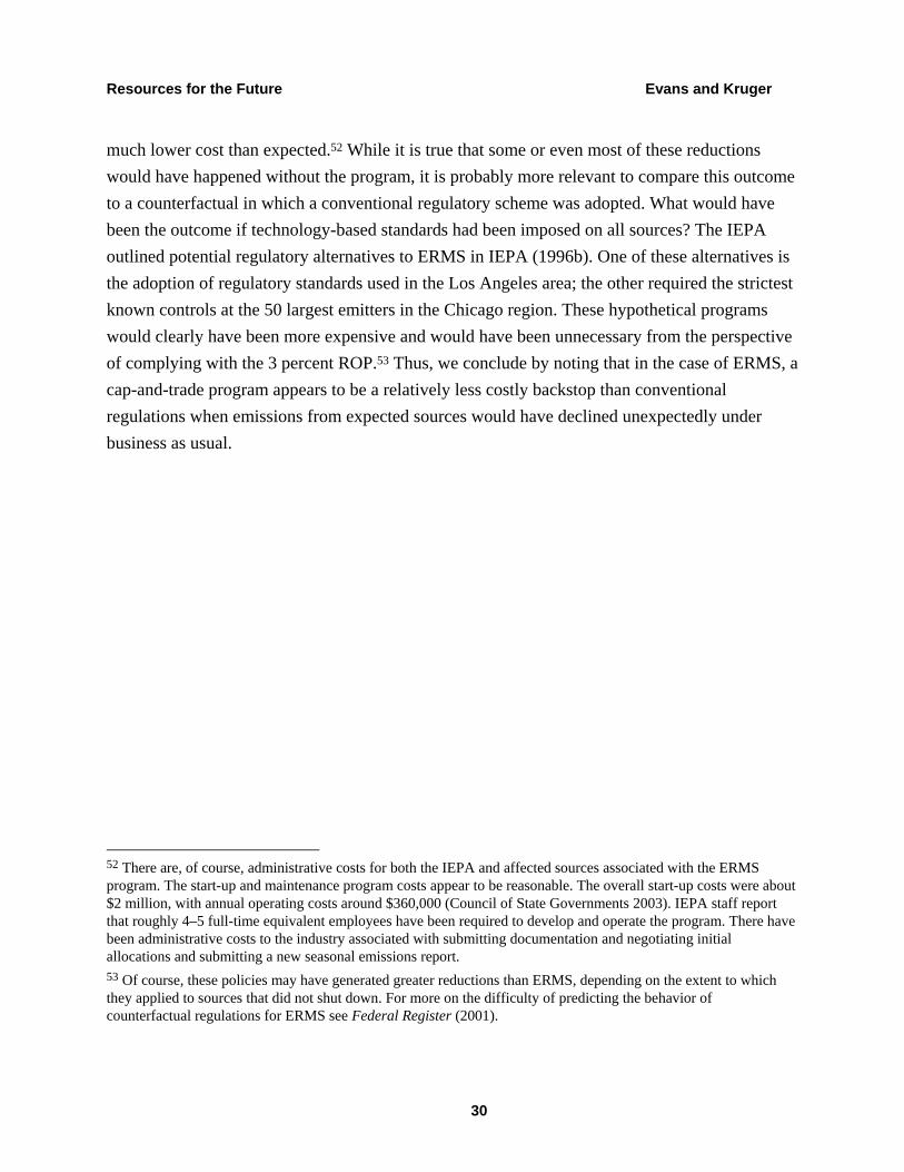
The electronic data available to analyze the program include source level seasonal emissions data from the ERMS Seasonal Emission Reports from 1998 to 2005. These data were provided by request from the IEPA. Table 1 summarizes the participation, emissions, and allowance allocation from the ERMS sources over this period.13 Reported emissions are far lower than allocations in all years. From 2000 to 2005 participating sources used 61, 52, 51, 44,
12 The utility of this banking restriction is debatable. It may help ensure that the region is in compliance with the ROP requirements by preventing substantial growth in emissions in a particular season. However, it does little to affect VOM emissions over timeframes critical for ozone control (days). At the same time, although it seems improbable that manufacturing in the region would swing so significantly to make this restriction even relevant, we do see allowances expiring due to source shutdown (see below). Furthermore, one unintended consequence of this restriction may be that it helps to reduce disagreement about what to do with banked allowances if allocations are adjusted in the future (IEPA 2001-2006). 13 The data reported here are slightly different from those reported in the IEPA’s annual ERMS reviews. This occurs for a variety of reasons. For example, there have been adjustments to emission reports and disagreements regarding emission reports between the IEPA and affected sources that are resolved after the reviews are released.

Resources for the Future Evans and Kruger
12
45, and 42 percent of their total allowance allocation. Despite the fact that there is no scarcity in the market, emissions are generally falling over time! As a consequence many allowances remain unused after their two-year lifetime and subsequently expire.
Table 2 summarizes total transactions, volume, and average allowance price as reported in the annual ERMS reviews. There have been relatively few ATU transactions between distinct sources. Allowance prices have been much lower than prices predicted prior to the advent of the program.14 IEPA (1996b) used cost data collected from the 15 percent ROP rule development, U.S.EPA abatement technology analyses, and proprietary information to develop representative abatement costs by SIC code and predicted a $285 ATU price (1996 $). Evans (1999) predicted allowance prices in the neighborhood of $1,000 per ATU (1999 $) using abatement cost data used to estimate the cost of the proposed RECLAIM VOM cap-and-trade program. In comparison, the average allowance price reported in 2005 was about $14 per ATU.
What explains the unexpected result that the ERMS cap was not binding and that allowance prices are essentially minimal? The following section explores competing hypotheses to explain why emissions are so far below allocations and examines the evidence.
3. Explaining Slackness in the ERMS Cap
3.1 Hypothesis #1: Inflation of Baseline
Recall that each source’s emissions baseline was determined from an average of the two highest summertime emissions from 1994 to 1996, with provisions for substituting other years if these three were not representative. If procedures to determine this baseline overstate the “typical” emissions from ERMS sources, then potentially there may be surplus allowances even with the 12 percent reduction from the baseline. Could this have contributed to the surplus of allowances in ERMS?
Several aspects of the process for setting baselines could explain the slackness of the ERMS cap. First, IEPA officials and company representatives say that in a few cases data for the
14 The realized allowance prices, particularly in later years, presumably solely reflect transaction costs as marginal abatement costs (given the performance standard restrictions) appear to be zero. A simple test of this hypothesis would be to see if total transaction prices are relatively insensitive to the number of ATUs transacted. Unfortunately we do not have transaction data.
Resources for the Future Evans and Kruger
13
baseline years were incomplete or based on rudimentary measurement methodologies.15 Although companies were required to report their VOM emissions during the base period through an annual emissions report, these data had not received much scrutiny prior to the process of determining each source’s allocation. Although it is impossible to judge whether all data are accurate, it is clear that the baseline emissions data received significantly more regulatory scrutiny under the allocation-setting process than they had in the past. The initial step in setting baselines was for the IEPA to provide each source with an estimate of its baseline. A source was then able to provide additional information to improve the estimate.
As with other trading programs, companies clearly had an incentive to document their emissions completely because higher emissions in the baseline years can translate into higher allocations (Montero et al. 2002). Thus, it is possible that the incentive for companies to better document their emissions data could have led to a higher baseline than was originally expected by regulators. On the other hand, there are some rules and incentives that counter this motivation. One important rule is that measurement techniques used to establish the baseline must be used for ERMS compliance, so higher allocations may simply be taken up by higher reported ERMS emissions. Secondly, sources may not want to avoid suggesting their sources emit more than the IEPA initially thought because such behavior may draw additional regulatory attention.
The ability to select the two years with highest emissions may also have an impact on the overall baseline as there is a convolution that “typical” emissions are somehow “high” emissions. Defined this way, the sum of “typical” emissions over each source may equal a level of emissions that is quite atypical for the entire region. To get a better sense of the influence of allowing the substituting of baseline years and averaging multiple years in the baseline, we looked at the ERMS allocation applications of 15 randomly selected full participants. Four of
15 A variation on this hypothesis is that measurement methodologies changed between the baseline period and the emissions-reporting period. For example, if sources revised their methodologies in ways that made emissions lower (e.g., changed to a lower emissions factor), this could explain the excess allowances. A few experts at the U.S.EPA and elsewhere were concerned that ERMS would suffer from an inflated baseline given the difficulty in measuring emissions (Evans 1999). Fears about the reliability of monitoring and measuring VOM emissions led to the abandonment of a VOM trading market under RECLAIM (Lents 2000; Thompson 2000). However, Illinois EPA officials noted that a source would need to adjust its baseline and thus allocations if it chose to use this new emissions factor, thereby preventing the generation of excess allowances from a methodology change. Also we note that ERMS emissions reports were subject to particular scrutiny of measurement techniques in the first few years of the program and, with the exception of sources that shut down, emissions have been relatively constant. This suggests that measurement techniques have been consistent. Furthermore, as it is clear that the cap is slack, a source’s incentive to try to apply a less stringent measurement methodology is relatively low.

Resources for the Future Evans and Kruger
14
these 15 sources used at least one year outside the 1994–1996 period as the basis for their emissions baseline. The justification for three of these sources was simply that sales were depressed and consequently alternative years ought to be used.
Given that the third baseline year likely had the lowest emissions (and ignoring the selection of alternative years), let us speculate that the year with the lower level of emissions among the two baseline years actually used is, in a sense, representative of all three years. The proposed baseline from these 15 sources is 5 percent (with a standard deviation of 3.4 percent) higher than emissions from the year with the second highest emissions.16 One can think of this statistic as a rough estimate of the baseline inflation that results from selecting a baseline from a number of years. The baseline would be even lower if shoulder years could not be used as a substitute. Unfortunately, we cannot make any more sophisticated hypotheses about the effect of alternative baseline calculations because we do not have reliable data on each source’s seasonal emissions for all years prior to 1998.
A third feature of the baseline-setting process was the ability of sources to request adjustments to baselines to get credit for voluntary overcompliance during the baseline period (provided such over compliance began post-1990). That is, baselines are generally based on allowable, not actual, emissions. IEPA officials noted that addressing source claims about voluntary credits was one of the most difficult parts of the baseline negotiation. Essentially, if companies were able to argue that their actual emissions were lower than their permit allowed, they received ATUs based on their allowable emissions.
To understand the significance of allocation for voluntary overcompliance, we looked at whether any of our 15 randomly selected sources had requested allowances for voluntary overcompliance.17 We examined “baseline request forms” for the 15 sources and found that 5 clearly requested additional allocations for over compliance. Over all 15 of the sources, they requested allocations at least 7 percent greater than their actual emissions. Despite this request for overcompliance, in total these sources actually received about 7 percent less than what they
16 Looking at variations in manufacturing data, the U.S.EPA predicted that the effect of this selection and averaging over multiple years would increase the cap by only .7 percent (Federal Register 2001). 17 Overcompliance is ubiquitous with command and control regulations. One hypothesis is that there is stochasticity in emissions so sources at any moment are typically overcomplying (Magat, Krupnick, and Harrington 1986). This suggests that if regulators wish to achieve a particular ambient outcome, they should take into account the deviation between allowable and actual emissions when developing a program to achieve further emission reductions.

Resources for the Future Evans and Kruger
15
requested. However, it is not clear that this difference in what the IEPA allocated is attributable to a rejection of the request for additional allowances due to overallocation. None of the 15 sources received exactly the baseline they requested; some received more allowances and some received fewer. The standard deviation of the percentage of allowances received to those allocated is 23 percent, so the adjustments made by the IEPA are often significant.18
How important was the baseline-setting process in contributing to the slack cap? We believe that incomplete or inaccurate emissions data, allowing the selection of the two highest years, and credit for voluntary overcompliance are significant contributors to the initial slackness in the ERMS cap.19 Further evidence that there is inflation in the baseline is that 1998 emissions would use only 67 percent of the total ATU allocation in 2000 (for those sources for which 1998 and 2000 data are available). In other words, two years before the ERMS program began, emissions were already 33 percent below the total 2000 allocation. The original intended start year for ERMS was 1999, so it is conceivable that there could be some early emission reductions in anticipation of the start date of the program. However, the magnitude of the gap between emissions and allowances, as well as our preceding analysis, indicates that early compliance is unlikely to explain much of the initial surplus of allowances.
Interestingly, none of the factors that inflated baselines would be significant to our discussion of the slack cap if the allocation process had been decoupled from the overall size of the cap. Other trading programs began with a fixed cap, and then allocated shares of the cap
18 We wanted to compare the baseline requests to the justification for the actual allocations the sources received as reflected in the IEPA’s “baseline determination letter.” However, despite the newness of the program and the pubic availability of these determination letters, they are only available in paper form and one must personally go through each source’s permit file to pull them out to copy. 19 Another allocation rule that may have resulted in baseline inflation is allowing some new emitting points (those permitted prior to May 1, 1999) to receive allocations. These new points may be replacing existing points. If both points, the original and replacement points, receive allocations, then there is overallocation. Although we do not know exactly (given data restrictions) whether these “pre-1999” new points displaced old ones, we have some idea as to their share of emissions from sources that also have points in operation from 1994 to 1996. In 2000, there were 178 tons of emissions from pre-1999 new points that did not yet have three years of operational data. This represents only about 3 percent of emissions from full participants in 2000. Of course, this small quantity of emissions could be displacing a much larger quantity. However, the sources that have such points used about 65 percent of their total allocation, representing 19 percent of the total allocation, in 2000. This is not much different than the ATU use of sources that do not have new points. Furthermore, the allowance use of these sources does not decrease substantially over time, suggesting that they are not displacing existing point emissions with new point emissions.
Resources for the Future Evans and Kruger
16
based on each source’s share of historic emissions.20 These other programs saw similar efforts to improve the accuracy of emissions baselines, to give flexibility on baseline years, and to address voluntary overcompliance but to the end of identifying a source’s share of the total cap. With the cap set first there is a zero sum game; if one source gets more, other companies will get less. In the case of ERMS, the absolute emission level was determined during the allocation process. To the extent that more emissions were “found,” there was a larger overall cap.
3.2 Hypothesis #2: Other Regulations
A second hypothesis for declining emissions and the subsequently nonbinding cap is that sources reduced their emissions to comply with other regulations, either actual or anticipated. As we discuss below, this theory has been advanced in the only other ex post analysis of the ERMS program of which we are aware. Potential sources of regulation that might have affected VOM emissions include (a) regulations promulgated by the state of Illinois for ozone compliance; (b) federal controls on HAPs; (c) regulations affecting new emission sources (new source review); (d) state and federal reporting requirements for HAPs; (e) existing and anticipated federal regulations affecting the VOM content of consumer products and coatings; and (f) voluntary reporting requirements for HAPs.
Kosobud et al. (2004) use a regression analysis to advance the theory that the “underlying layer” of conventional regulation is the primary cause of low allowance prices and expiring allowances in the system. The authors argue that such regulations explain why individual sources do not emit up to their individual allocations.21 However, this claim is made absent identification of any regulations promulgated after the baseline period that might affect current emissions. Indeed, the IEPA has not adopted any regulations affecting VOM emissions from ERMS sources since the program was adopted in 1997.22
20 For example, in the SO2-trading program, baseline adjustments for forced outages, as well as allocation formulas within Title IV of the Clean Air Act, would have led to about a 9 percent increase in the SO2 cap had there not been a ratchet (McLean 1996). This feature, sometimes known as a “compliance factor,” was also present in allowance allocation methodologies put forward in some Member State National Allocation Plans in the EU ETS. 21 In some sense this argument is undeniable; if command and control regulations are taken away, emissions would likely rise. However, ERMS is intended to reduce emissions beyond what would be realized if only command and control rules in place during the baseline were enforced. 22 Also note that the statistical analysis in Kosobud et al. (2004) is limited to those sources that engage in trades, which is an indirect way of explaining why the cap is slack.
Resources for the Future Evans and Kruger
17
If sources were required to comply with HAPs technology-based standards that affect VOMs then this could have led to an overall level of emissions below the ERMS cap.23 Both industry and IEPA officials we interviewed maintained that existing HAPs regulations were not primarily responsible for the decline in emissions under ERMS. However, a check of the federal schedule for the promulgation of HAPs rules reveals that most of the 70 or so HAP regulations that come into effect from 1997 to 2007 affect VOM emissions (U.S.EPA 2006). For example, Hazardous Organic NESHAP (the “HON Rule”), when finalized in 1994, was expected to reduce national VOM emissions by 1 million tons annually (U.S.EPA 2000). Sources were not required to comply with this rule until 1998, after baseline emissions were determined. These HAP regulations typically affect sources annually emitting 10 tons of any one of the 188 regulated HAP pollutants or 25 tons of these HAP pollutants.
Moreover, IEPA officials and some company representatives noted that the anticipation of future federal regulations could have affected emissions. One company official said that his company starts planning for compliance once a regulation is proposed. Another industry representative indicated that his facility adopted a leak detection system, which led to VOM reductions, in anticipation of a federal requirement for such a system for smaller chemical production facilities. An official of a different company noted that expectations about future regulations were sometimes built into capital expenditures. In some cases, these could have been specific proposed future regulations, but in other cases it could have been a more general sense that regulations would eventually be tighter. An IEPA official agreed that as companies “swap out” manufacturing equipment, they sometimes also make environmental improvements to address future regulations. He noted that this happens, for example, in the printing industry where capital turnover is rapid.
Unfortunately, knowing which ERMS sources are affected by the HAP rules is difficult. This is because the IEPA does not know for certain if a source is affected by a particular rule until the source goes through a CAAPP permitting process (either a new permit or a renewal). The promulgation of a HAP rule is not cause to reassess the permit of any source that may be affected. However, despite the rule not being identified in its operating permit, the source is still responsible for complying with a rule if the source fits the applicability criteria of the rule on the date the rule goes into effect.
23 Note that the technologies that abate HAP VOMs often do not discriminate. When used, they also abate non-HAP VOMs that are present with the HAP VOMs.

Resources for the Future Evans and Kruger
18
However, we can estimate the effect of these HAP rules on emissions from ERMS sources by considering whether a source is likely to be affected by one of these rules. The source must fit two criteria. First, it must be part of an industry that is likely to be affected by one of the rules. Second, it must be likely to have an emissions level that meets the applicability threshold. During each HAP rulemaking the U.S.EPA typically identifies those industries, identified by their four-digit SIC code, most likely to be affected by the rule. (However, applicability will depend ultimately on a source’s production processes.) A compilation of these SIC codes for each HAP rule was provided to us by the U.S.EPA, and the IEPA provided us with the SIC code for each affected source. Recall that typically only sources with annual emissions of 25 total tons or 10 tons of one HAP pollutant are affected by the HAP rules. We only have access to source-level seasonal HAP emissions data from 2001 to 2005, so the emissions are scaled to an annual basis. Provided it is in one of the likely affected industries, we assume that if a source meets either of the HAP emissions thresholds in any year it may be affected by a HAP rule.
To roughly estimate the effect of these HAP rules we use a regression with annual emissions (by 200 pound, one ATU, increments) as the dependent variable. The independent variable of interest is a dummy variable indicating whether the source must (likely) comply with at least one of the rules within two years. We assume that the rule begins to affect source behavior two compliance periods in advance based on comments from representatives of regulated sources. Additional explanatory variables include year dummies and firm fixed effects. Only those sources for which we have seasonal data from 1998 to 2005 are included in the analysis, which is reported in Table 3.24
We see that the coefficient on the variable RULE is negative and suggests that allowance use falls by about 125 ATUs per year for those sources likely affected by a HAP rule. There are 6 sources affected by a rule in 2000, rising to 20 sources by 2005. So, the sources in the sample used about 750 fewer allowances in 2000 and about 2,500 fewer allowances in 2005. The sources in the sample used about 5,000 fewer allowances from 2000 to 2005, so our rough estimate suggests that in 2005 about a third of the reduction in allowance used by these sources is due to HAP rules.
24 For a description of these sources see the following section on source shutdowns. The sources that have not shut down comprise the majority of emissions and individual sources operating in the program. Of course, to the extent that the HAP rules promote source closure, eliminating the shutdown sources may result in any underestimate of the total effect of these rules.
Resources for the Future Evans and Kruger
19
Is it also possible that capital turnover triggered regulatory requirements that led to additional reductions in emissions? New sources are subject to tighter performance standards than existing sources, so as capital turns over emissions are ratcheted downward presuming production does not increase substantially.25 The evidence suggests otherwise. Any new source permitted prior to May 1, 1999, but not in existence in the baseline period may receive allocations. These new emission points require three years of operational data before they receive allocations, so if such sources exist they are typically identified in the seasonal data. However, these emissions do not seem to be displacing emissions from existing points (see footnote 19). Second, emissions are not declining significantly after 2000 for those sources that do not shut down, suggesting that sources of emissions existing in the baseline period are not being displaced significantly. Finally, major new sources must use 1.3 allowances for every 200 pounds of VOMs emitted, and only 0.1 to 17 tons of total emissions, depending on the year, are subject to this requirement.
Under section 183(e) of the 1990 Clean Air Act, the U.S.EPA was charged with developing national standards for VOMs from commercial and consumer products that account for at least 80 percent of VOM emissions on a reactivity-adjusted basis in areas not in compliance with the ambient ozone standard. The U.S.EPA was provided a choice to regulate the VOM content of these products, or develop guidance for the control of VOM emissions from the use of these products (Federal Register 2005).26 The first of these rules was adopted in 1998. The input requirements presumably have an affect on the emissions from both the end user and the producer of these products.27, 28 Could these regulations have an impact on emissions at sources affected by ERMS? Promulgation of these regulations began in the mid-nineties and
25 As VOM emissions typically represent lost product or input, it is also possible that VOM emissions would simply fall with efficiency gains from capital turnover. 26 It appears that in cases where a NESHAP rule is already affecting a particular source of end user (such as wood furniture coaters), the U.S.EPA has taken the route of providing control guidance. 27 One company representative mentioned that his firm was producing products with less VOM content due to changes in the demands of the consumers, which in part were motivated by Occupational Safety and Health Administration regulations regarding the combustibility of inputs. 28 Although not all VOM-containing products have been regulated federally, the influence of state regulations may be having a similar effect. For example, sources in many regions are subject to tight limitations on the VOM content of the coatings they use. This would expand the market for VOM coatings and potentially influencing emissions from end-users (if the low-VOM coatings are cost/performance-comparable) or the producers of these products (by lowering the use of VOM feedstocks).
Resources for the Future Evans and Kruger
20
started to become effective in the late nineties. Thus, we might expect that their effect is absent in both the baseline and the compliance period.
Alternatively, could reporting requirements for toxic emissions have led sources to voluntarily or preemptively reduce their emissions?29 Two different reporting requirements affect sources in ERMS. The first is the Toxics Release Inventory (TRI), which began in 1988 and is administered by the U.S.EPA.30 The second set of requirements is from the IEPA, which began requiring sources to report hazardous emissions that are also VOMs on annual and ERMS reporting forms in 2001.
Given data limitations, it is difficult to test for the influence of hazardous emissions disclosure on emissions. However, there are a few reasons to believe that the voluntary aspect of hazardous emission reporting does not explain why the ERMS cap is slack. First, as the TRI program started in 1988, many of the low-cost reductions presumably occurred well before the start of the ERMS program (although the TRI may then be explaining overcompliance in the baseline). Second, although hazardous emissions must be reported to the IEPA, it is difficult to claim that they are truly disclosed at the source level as these data are not easily accessible to the public. Finally, none of the industry officials we interviewed said that TRI or the IEPA HAP reporting requirements were a major factor in VOM reductions at their companies.
3.3 Hypothesis #3: Industry Contraction
Could the dramatic drop in emissions be explained by economic conditions in the industries affected by the ERMS program?31 If facilities in the region shut down or reduced production, and if there were not a significant number of new facilities, this could explain the lack of demand for allowances and the subsequent surplus.
Before exploring this hypothesis, it is necessary to know how shutdowns of facilities are treated. In ERMS, facilities continue to receive 100 percent of their allowances if they shut
29 The justification for disclosing toxic emissions is to provide communities with information on surrounding environmental hazards and to encourage emissions reductions through anticipated or actual community pressure (Weil et al. 2006; Hamilton 2005). 30 There is mixed evidence as to whether TRI itself can be credited for the reported reductions in hazardous emissions after its adoption (Weil et al. 2006; Hamilton 2005). 31 No attempt is made here to identify the source of any industry contraction. However, hypotheses include economic downturn (as with RECLAIM, see Klier et al. 1997) and differential treatment of industry inside and outside nonattainment areas (Henderson 1996).

Resources for the Future Evans and Kruger
21
down. If these allowances are not used within a year, 20 percent of them are confiscated and provided to the ACMA. This provision was incorporated into ERMS to prevent the cap from shrinking, as new sources are not provided their own allocation (IEPA 1996a).
The policy of continuing to allocate allowances after the closure of a facility is a feature of other U.S. trading programs, but generally not in the EU ETS (Ahman et al. 2005). Although it may seem counterintuitive to continue to distribute allowances to a facility that does not operate, there is an important economic rationale for this provision. If allowances are confiscated, an incentive exists to continue the operation of old and inefficient facilities. Essentially, by tying allocation to operation, allowances become a subsidy for the continued operation of a facility (Baumol and Oates 1988; Kling and Zhao 2000).32
Shutdowns have had a significant effect on emissions under ERMS. In 2005, thirty-six facilities with no emissions continued to receive allocations.33 In contrast, only 9 new facilities entered the program between 2000 and 2005. As described below, Figure 1 confirms that source shutdowns play a large role in emission reductions and consequently the additional slackness in the cap, after 2000. However, source shutdowns do not explain why a large share of the allowances remained unused in 2000.
We see in Figure 1 the influence of source shutdowns on the share of the total ATU allocation retired for compliance each year. The solid line represents the share of the allocation used by all existing, new, and shutdown full participants in each period. These data are taken from Table 1, assuming that the hypothetical allocation in 1998 and 1999 is the same as in 2000. Note that only 62 percent of the total allowance allocation is used in 2000 and that this percentage falls in 2001. It drops again in 2003 and by 2005 is about 42 percent.
The dotted line represents the share of their own allowance allocations used by sources that reported their emissions in 1998 and 1999, received allowances in 2000 and shut down by 2005 (i.e., they have an allocation, but no emissions), and five other sources with special
32 One way to avoid an indefinite allocation of the property right to pollute without adversely affecting a source’s shutdown decision is to auction the allowances (Kling and Zhao 2000). 33 It clearly would be more informative to perform this analysis at the point level, because then we might see if economic pressures are also driving emission reductions at individual sources, either by points being shut down or used less extensively.

Resources for the Future Evans and Kruger
22
circumstances that make them more like shutdown sources.34 In 2000, these sources used about 50 percent of their allocation. We see that as they are shutting down, the share of allocations used by these sources drops dramatically over the six-year period the program is in place. Furthermore, these sources represent a nontrivial share, about 28 percent, of the total allocation in all six years.
In contrast to the large number of shutdowns starting in 2001, there are very few source shutdowns prior to 2001. In 2000, only five sources with no emissions continued to receive allocations. These sources received a collective allocation of 958 ATUs, which represents only 3 percent of the unused allowances allocated in 2000.
To what extent are shutdowns driving the increased slackness in the allowance cap after 2000? Answering this question requires an assumption about how many ATUs these shutdown sources would have used if they had continued to operate. For this, we look at the share of allowances used by sources that were in the program and operated in each of the six years (and reported emissions in 1998 and 1999). The long dashed line represents these sources. There are 133 such sources and they received about 69 percent of the total ATU allocation in each year.35 Their emissions as a share of their allocations in 2000 is 70 percent, which declines to 58 percent by 2005.36 Figure 2 uses data from these sources that do not shut down to show how emissions are considerably lower than allocations across all industry types in the ERMS program.37
34 One of these sources shut down, but then a small portion of the source was bought, along with most of its allocation stream, and began emitting again in 2003 (although at only 10 percent of its allocation). Similarly, two of the other sources were commonly owned and both closed; however, about a third of their allocation stream was sold to a new participating source that only uses about 15 percent of it. 35 About 4 percent of the allocation each period went to sources that did not shut down, did not emit all six years, or for which we have no 1998 or 1999 seasonal emissions data. These sources either received a CAAPP permit after 2000, are new, changed their participation status, or changed their permitting status (either from a CAAPP to another permit type or vice versa). Furthermore, the percentages in Figure 1 do not take into account allocations to ERGs (some of which are sources that shut down that would have been ERMS participants) or the unused allowances confiscated from shutdown sources. 36 One hypothesis we did not explore is whether some underlying cause of source shutdown, say reduced economic activity in the relevant sectors, is also influencing emissions from sources that have remained in existence. 37 It is not enough to claim that because ATU use as a share of total allocations is relatively constant over time, the behavior of individual sources is typically invariant over time. To investigate the behavior of individual sources, using OLS we regressed the log ratio of source’s annual emissions to its ATU allocation on source fixed effects and year dummies. The R2 of this regression is .89. This implies that a large share of the variation in allowance use can be identified with these variables so we can be comfortable that there is significant consistency over time in the behavior of individual sources.
Resources for the Future Evans and Kruger
23
The mixed-interval line shows the share of the total allocation used in each period assuming that shutdown sources use their allocation at the same rate as the sources that emit all six years.38 We can now clearly see that source shutdowns explain the vast majority of the reduction in allowance use after 2000.39 In reality, 2005 emissions are 71 percent of 2000 emissions, but in the counterfactual (i.e., no shutdown) case, they are 89 percent of 2000 emissions. So we can attribute 62 percent of the emission reduction from 2000 to 2005 to source shutdown. In terms of ATU use, in 2005 about 25 percent of the unused ATUs, accounting for 14 percent of the total cap, are attributable to source shutdown given our assumed counterfactual.
3.4 Hypothesis #4: Market Behavior and Uncertainty
Emissions trading is based on the idea that firms will not only seek out the lowest cost options from their own facilities but will also make investments to sell or buy allowances from other firms if the expected allowance price is above or below their own marginal cost of reductions. This tenet of emissions trading is based on several assumptions. First, firms minimize their total compliance cost, which is the sum of their abatement cost and the cost of trading. Second, firms are confident in the validity of the program and can rely on institutions to ensure a liquid and dependable market to provide allowances currently and in the future. Finally, firms have good knowledge about the cost of reductions at other firms and about current and expected future prices in the allowance market. That is, they have a reasonable idea of their position in the market. Each of these assumptions may be violated under ERMS and may contribute to the allowance surplus, but the relative importance of these violations is very difficult to quantify.
The incentives of company staff making environmental compliance decisions may not be consistent with minimizing the cost of abatement. This may occur because the environmental manager is unwilling to bear the risk of relying on the market for compliance. That is, the risk to the individual may exceed the risk to the source of being caught short of required allowances. Alternatively, the explanation could simply be inertia in firm structure. Both industry and IEPA officials emphasized that a combination of these factors made some firms reluctant to depend on
38 Emissions from new entrants are not included in these hypothetical shares. ATU use from new entrants is quite low, at most 2 percent of total emissions. Adding them back in would make the decline in ATU use as a percentage of allocation even less significant. 39 Presumably, these shutdowns have nothing to do with the ERMS program, particularly considering the low emission reductions required of ERMS and that almost all of them occurred after ERMS came into effect.

Resources for the Future Evans and Kruger
24
allowances for compliance.40 It is also possible that sources do not engage in the market because they are concerned about the viability of the ERMS program or that other regulations would be adopted that would disrupt their compliance strategy.41 The delays, changes, and uncertainties surrounding the start-up of the ERMS program may have further discouraged sources from fully engaging in the ERMS market.42
The last condition for efficient market behavior, that is, that sources must know their position in the market, might be relevant to the ERMS mystery. As noted above, the allowance price expected by the IEPA was significantly greater than what was realized in the market. Expecting a higher price, sources may have overinvested in abatement techniques, leading to more emissions abatement than is socially optimal and subsequently lower allowance prices and emissions. This is a great irony of emissions trading. Although the benefits to emissions trading are ostensibly the greatest when sources are more heterogeneous and their costs more opaque to regulators, the heterogeneity itself likely implies significant opaqueness for participants in the market. Sources may not be able to identify their appropriate position in the market, at least at its outset.43 None of these explanations, however, satisfactorily explains why emissions continue to be so far below allocations.
Once the market gets going, however, the price (both spot and forward) is the only signal required, provided there is sufficient market activity. Even if these sources anticipated selling allowances, economic theory would suggest that with very low ATU prices, sources might decide to emit more to reduce variable costs associated with reducing emissions. Sources also have built banks they can rely on if they find themselves unexpectedly short of ATUs. Certainly other emissions-trading markets have reacted this way when prices have fallen (Ellerman et al.
40 Industry officials noted that some firms are reluctant to depend on allowances for compliance either because they don’t have the expertise to take advantage of trading or because they are reluctant to rely on the market for compliance given regulatory and other uncertainties. For example, one said that his company would not depend on going to the market to address future growth and would handle compliance within the company. IEPA officials believe that, in general, many companies did not want to be in position of buying ATUs because there was great fear that there wouldn’t be adequate supply. They reiterated that the purpose of ACMA was to allay fears that the “market would be a desert.” 41 This may result in what economists call “autarkic compliance” (Foster and Hahn 1995; Tripp and Dudek 1989). That is, a situation in which sources simply do not engage in the market and prefer to “go it alone.” 42 See IEPA (2001) for details on the regulatory uncertainty surrounding the ERMS program. 43 Admittedly, this does not necessarily imply that sources more often expected to be sellers in the market. However, one can imagine that given the asymmetric costs of being short allowances (regulatory penalties, greater regulatory attention in the future), it is easier to make compliance decisions assuming one may sell allowances.
Resources for the Future Evans and Kruger
25
2000; Burtraw and Evans 2004). However, we do not see this behavior in the EMRS market, so we suspect that this source of market inefficiency is not contributing to the allowance surplus.44
3.5 Hypothesis #5: Innovation and Managerial Empowerment
The economics literature generally holds that market-based approaches to regulation such as taxes or tradable allowance programs have a greater impact on innovation than do conventional technology standards (Jaffe et al. 2003; Sterner 2003). The additional innovation expected by the economics literature requires a price signal that indicates scarcity of emission allowances. The scarcer allowances are, the higher the price and the greater the incentive to innovate. The reductions required of sources were not that significant, so the innovation incentive prior to the advent of the program, when the expected allowance price was nontrivial, was likely weak.
Porter and others in the business school literature have stressed that the flexibility inherent in emissions trading can be used to encourage firms to operate more efficiently, such that environmental regulations may even pay for themselves (Porter and van der Linde 1995). Unfortunately, rarely do such observers identify specific conditions under which they expect such situations to occur (Palmer et al. 1995). However, perhaps environmental compliance managers are limited in the activities that they can engage in due to inefficiencies in firm structure. A cap-and-trade program might identify these inefficiencies and empower environmental managers to take a more holistic view of the production process, identify places where inputs are lost, and improve production efficiency. Once let loose on the entire production process, managers identify enough input savings that the cap becomes unnecessary.45 Industry and government officers said that they believed that the flexibility of the program led to the identification of numerous low-cost abatement options, but there is little evidence that this is the case.
44 It is possible, but we do not know how likely, that a source that overcomplied in the early years may find difficulty in reversing its compliance decision. For example, perhaps the source installed an abatement device or made substantial process changes. Contributing to this irreversibility is the possibility that the compliance method is now integral to the source’s operating permit. Unfortunately we cannot easily identify which permits incorporate voluntary compliance methods as a result of ERMS because the CAAPP permit program started at the same time. 45 Note the competing view of the environmental manager/compliance officer compared to Hypothesis 4. Here, they are a neglected and untapped resource. In Hypothesis 4, their self-interest might be so poorly aligned with the interest of the firm that they engage in autarky.

Resources for the Future Evans and Kruger
26
4. Conclusions/Additional Program Experience/Lessons
As we have discussed, a number of factors could have contributed to the lack of scarcity in the ERMS program. However, we have identified three important causes. At the beginning of the program, a generous allocation of ATUs to address voluntary overcompliance and other baseline concerns, clearly contributed to an overall allocation that was higher than emissions. In addition, HAPs regulations that came into effect after the baseline period also contributed to lower than expected emission levels. This overallocation might have been a transitory condition if it was followed by production and emissions growth in the following years so that eventually the increased demand for allowances led to a binding cap. However, a third factor, the significant number of shutdowns that began in 2000, led to a continued drop in emissions. As we have shown, these shutdowns reduced ATU use by an additional 14 percent by 2005. This combination of factors has essentially made the ERMS cap irrelevant as an emissions reduction mechanism.46
The ERMS case points to the challenges of setting the “right” target in an emissions-trading program.47 One of the most difficult analytical aspects associated with the design of an emissions-trading program is projecting what would happen without the program (sometimes known as the “counterfactual” or “business as usual” case). This is particularly true where emissions-trading programs address diverse sources in multiple industrial sectors. In such cases, it is difficult to predict how economic changes might affect a wide variety of industries and product lines. Models used to project the business as usual case for ERMS were relatively basic, and could not have anticipated the number of shutdowns that would result in the early years of the program.
Furthermore, where emissions reductions are relatively small on a percentage basis, there is potentially less room for error in calculating a business as usual case and the needed reductions. For ERMS, the relatively modest reduction from baseline emission levels meant that if baseline emissions were significantly overestimated or if the impact of shutdowns was
46 Similarly, voluntary shutdowns, increases in control efficiencies, and new federal HAP regulations accounted for over a third of the required reductions for the 15 percent ROP rule (IEPA 1996b). 47 We do not address the question of whether the ERMS target was justified from a cost and benefit perspective. Although we have not assessed this aspect of the ERMS program in this paper, it is important to remember that this is a critical piece for judging the program’s overall performance.
Resources for the Future Evans and Kruger
27
significantly underestimated, then there was a chance that the cap would not bind. This same set of conditions might not have the same effect in a program with a larger emission reduction.
In addition, compared to the emissions data for electric power plants covered in the U.S. SO2 program, emissions data used for the development of ERMS were poor and much less transparent. The dearth of data on actual emissions highlights an important drawback faced when developing regulations in general. Ultimately, one lesson from ERMS is that no matter what abatement strategy is being contemplated, it is important to get a measurement program into place quickly to get an accurate baseline.48
Starting with a fixed quantity of allowable emissions would help avoid the apparent “baseline inflation” that occurred with ERMS. If the emissions target is set at the beginning, then any adjustments for overcompliance or to address individual baseline year anomalies becomes a case of dividing the pie rather than making the pie bigger. If there are more claims for allowances than anticipated, there can be a “ratchet” of the overall allocation whereby every source’s allocation is adjusted downward to maintain the size of the cap. This type of cap-setting procedure is similar to the methods used in the SO2 program and in some member states in the EU ETS. For achieving a particular environmental outcome, this is preferable to the procedure in the ERMS program, in which adjustments to source baselines were made before the size of the overall cap was determined.
Mechanism to Address Unexpected Outcomes
The recent price drop and lower than expected emissions levels in the EU ETS are not the first unexpected outcomes in an emissions-trading program. For example, both the NOX Ozone Transport Commission and RECLAIM markets were marked by unexpected price spikes (Kruger and Pizer 2004; Burtraw et al. 2005). The ERMS case provides further evidence demonstrating the need for institutions and mechanisms that respond to new information or adjust to unexpected outcomes.49 In most cases, these types of mechanisms are discussed in the context of addressing the possibility of higher, as opposed to lower, than anticipated prices. For example, Pizer (2002)
48 There is actually a significant dearth of reliable electronic data for ERMS. Presumably it would be much easier to understand the performance of the program and to evaluate emission reports (to check for consistency in measurement techniques, for example) if information were reported electronically. 49 Here we are discussing these types of mechanisms in general and not necessarily in the context of ERMS, where statutory restrictions may limit their introduction.
Resources for the Future Evans and Kruger
28
suggests a “safety valve” mechanism whereby a regulated facility would be able to purchase additional allowances at a set price. Bluestein (2003) proposes a “circuit breaker” in which allowance allocations decline over time, but the decline would be halted if allowance prices exceeded a certain level.
Approaches could also be introduced to ensure that prices are not “too low.” The economic rationale for this type of mechanism is that a price floor would improve economic welfare.50 On the other hand, this type of mechanism might create implementation difficulties, as it would require governments to intervene in markets by buying up or confiscating excess allowances. However, Hepburn et al. (2006) suggest that a floor price could be created by the use of a minimum bid price auction. Sources would indicate offer prices for different quantities of allowances in the auction. If the clearing price for the auction were too low, the number of allowances being auctioned would be reduced until an acceptable clearing price was realized.
Ultimately, mechanisms to ensure a minimum allowance price might not be necessary to ensure near-term allowance scarcity if there is a banking mechanism and there is a general expectation that abatement costs will increase and allocations will decrease in the future. In other words, overallocation is less of a problem if expectations of higher prices in the future lead firms to abate in the present and bank allowances for future use (by allowing banking, future allowance prices would be lower but current prices would be higher). In this sense, ERMS and the EU ETS have the opposite problem. In the case of the EU ETS, there is an expectation that there will be higher demand for allowances in the second phase of the program, which begins in 2008. However, allowances banked in the first phase of the program may not be held for use in the second phase. On the other hand, there is a banking mechanism in ERMS that despite being somewhat restrictive should nevertheless allow current emission reductions to be held for future use in the form of banked allowances. However, there is no apparent prospect of significant
50 In other words, if pollution causes damage yet is not scarce, that is, the price is zero, then emissions should be reduced in order to improve welfare. Note, however, that we are abstracting from the actual situation in ERMS where there are also regulatory standards that may bind.

Resources for the Future Evans and Kruger
29
growth in emissions demand in ERMS or the anticipation of future higher prices.51 Thus, there is no incentive to reduce current emissions to maintain a bank. Instead, sources have allowed a significant number of allowances to expire. ERMS therefore appears to be something of an anomaly—a cap-and-trade program in which emissions appear to have stabilized, at least for the immediate future—without the help of a cap.
Finally, when examining approaches to limiting price or emissions uncertainty in emissions-trading programs, we find that several of the classic environmental instrument questions are as relevant as ever. What levels of emissions reductions are necessary to meet an environmental goal? When do those goals need to be met, that is, in the short term or the long term? What level of cost is justified by the environmental benefits of reduction? What cost is politically feasible? The answers to these questions might be very different for different environmental problems and might lead policy makers to adopt different approaches to addressing uncertain outcomes in cap-and-trade programs.
Was the ERMS Program a Success?
The ERMS program does not fit the textbook model of how a trading program should behave. The purpose of an emissions-trading system is to ration a scarce good efficiently. Clearly VOM emissions are not scarce in this market given the vast amount of banked ATUs expiring and the minimal price for ATUs. It is also clear that the cap-setting and allocation processes contributed to this outcome.
On the other hand, it is important to remember that the emission reduction objectives of the ERMS program were met. It was the IEPA’s obligation to comply with the 3 percent ROP plan, not to achieve an efficient level of VOM emissions with a cost-effective regulatory instrument. Reductions were achieved well beyond the objectives of the program and likely at a
51 This could change, of course, if the IEPA decides to lower the ERMS cap to meet the new 8-hour ozone standard, as it is strongly considering (IEPA 2006). There are numerous issues to address if the cap is to be adjusted. The obvious one is whether all sources should be treated alike when adjusting allocations; in particular, whether shutdown sources and sources that have and will be affected by NESHAP standards will be treated the same as the other sources. Furthermore, there is the question of what to do with the allowances currently in the ACMA (which have an indefinite life). There is also the matter of the push toward regulating VOMs based on their potential to create ozone, that is, their reactivity (for a discussion on the challenges in modifying ERMS to account for reactivity, see Solomon and Gorman 1998). A cap-and-trade program with trading ratios has the ability to explicitly capture differences in reactivity, but again, adjusting allocations to this end may be challenging.
Resources for the Future Evans and Kruger
30
much lower cost than expected.52 While it is true that some or even most of these reductions would have happened without the program, it is probably more relevant to compare this outcome to a counterfactual in which a conventional regulatory scheme was adopted. What would have been the outcome if technology-based standards had been imposed on all sources? The IEPA outlined potential regulatory alternatives to ERMS in IEPA (1996b). One of these alternatives is the adoption of regulatory standards used in the Los Angeles area; the other required the strictest known controls at the 50 largest emitters in the Chicago region. These hypothetical programs would clearly have been more expensive and would have been unnecessary from the perspective of complying with the 3 percent ROP.53 Thus, we conclude by noting that in the case of ERMS, a cap-and-trade program appears to be a relatively less costly backstop than conventional regulations when emissions from expected sources would have declined unexpectedly under business as usual.
52 There are, of course, administrative costs for both the IEPA and affected sources associated with the ERMS program. The start-up and maintenance program costs appear to be reasonable. The overall start-up costs were about $2 million, with annual operating costs around $360,000 (Council of State Governments 2003). IEPA staff report that roughly 4–5 full-time equivalent employees have been required to develop and operate the program. There have been administrative costs to the industry associated with submitting documentation and negotiating initial allocations and submitting a new seasonal emissions report. 53 Of course, these policies may have generated greater reductions than ERMS, depending on the extent to which they applied to sources that did not shut down. For more on the difficulty of predicting the behavior of counterfactual regulations for ERMS see Federal Register (2001).
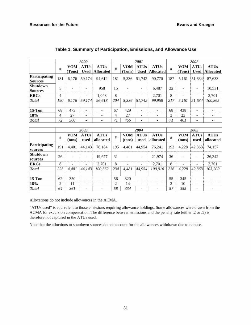
Resources for the Future Evans and Krueger
31
Table 1. Summary of Participation, Emissions, and Allowance Use 2000 2001 2002 # VOM
(Tons) ATUs Used
ATUs Allocated # VOM
(Tons)ATUsUsed
ATUs Allocated # VOM
(Tons) ATUsUsed
ATUs Allocated
Participating Sources 181 6,176 59,174 94,612 181 5,336 51,742 90,770 187 5,161 51,634 87,633
Shutdown Sources 5 - - 958 15 - - 6,487 22 - - 10,531
ERGs 4 - - 1,048 8 - - 2,701 8 - - 2,701 Total 190 6,176 59,174 96,618 204 5,336 51,742 99,958 217 5,161 51,634 100,865 15-Ton 68 473 - - 67 429 - - 68 438 - - 18% 4 27 - - 4 27 - - 3 23 - - Total 72 500 - - 71 456 - - 71 461 - -
2003 2004 2005 # VOM
(tons) ATUs used
ATUs allocated # VOM
(tons) ATUsused
ATUs allocated # VOM
(tons) ATUsused
ATUs allocated
Participating sources 191 4,401 44,143 78,184 195 4,481 44,954 76,241 192 4,228 42,363 74,157
Shutdown sources 26 - - 19,677 31 - - 21,974 36 - - 26,342
ERGs 8 - - 2,701 8 - - 2,701 8 - - 2,701 Total 225 4,401 44,143 100,562 234 4,481 44,954 100,916 236 4,228 42,363 103,200 15-Ton 62 350 - - 56 320 - - 55 345 - - 18% 2 11 - - 2 14 - - 2 10 - - Total 64 361 - - 58 334 - - 57 355 - -
Allocations do not include allowances in the ACMA.
“ATUs used” is equivalent to those emissions requiring allowance holdings. Some allowances were drawn from the ACMA for excursion compensation. The difference between emissions and the penalty rate (either .2 or .5) is therefore not captured in the ATUs used.
Note that the alloctions to shutdown sources do not account for the allowances withdrawn due to nonuse.
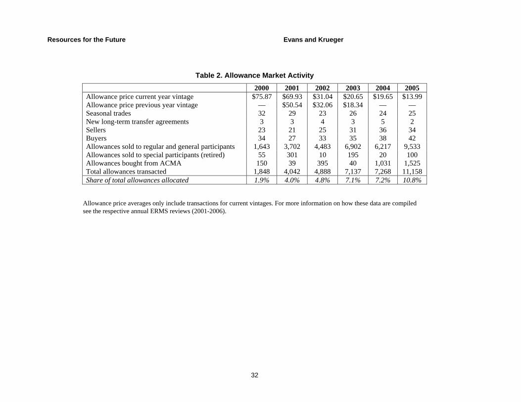
Resources for the Future Evans and Krueger
32
Table 2. Allowance Market Activity 2000 2001 2002 2003 2004 2005 Allowance price current year vintage $75.87 $69.93 $31.04 $20.65 $19.65 $13.99 Allowance price previous year vintage — $50.54 $32.06 $18.34 — — Seasonal trades 32 29 23 26 24 25 New long-term transfer agreements 3 3 4 3 5 2 Sellers 23 21 25 31 36 34 Buyers 34 27 33 35 38 42 Allowances sold to regular and general participants 1,643 3,702 4,483 6,902 6,217 9,533 Allowances sold to special participants (retired) 55 301 10 195 20 100 Allowances bought from ACMA 150 39 395 40 1,031 1,525 Total allowances transacted 1,848 4,042 4,888 7,137 7,268 11,158 Share of total allowances allocated 1.9% 4.0% 4.8% 7.1% 7.2% 10.8%
Allowance price averages only include transactions for current vintages. For more information on how these data are compiled see the respective annual ERMS reviews (2001-2006).
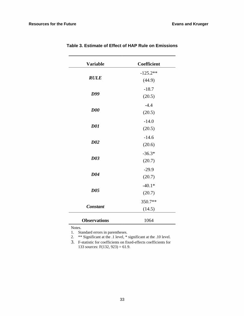
Resources for the Future Evans and Krueger
33
Table 3. Estimate of Effect of HAP Rule on Emissions
Variable Coefficient
RULE -125.2**
(44.9)
D99 -18.7 (20.5)
D00 -4.4
(20.5)
D01 -14.0 (20.5)
D02 -14.6 (20.6)
D03 -36.3* (20.7)
D04 -29.9 (20.7)
D05 -40.1* (20.7)
Constant 350.7** (14.5)
Observations 1064 Notes. 1. Standard errors in parentheses. 2. ** Significant at the .1 level, * significant at the .10 level. 3. F-statistic for coefficients on fixed-effects coefficients for
133 sources: F(132, 923) = 61.9.
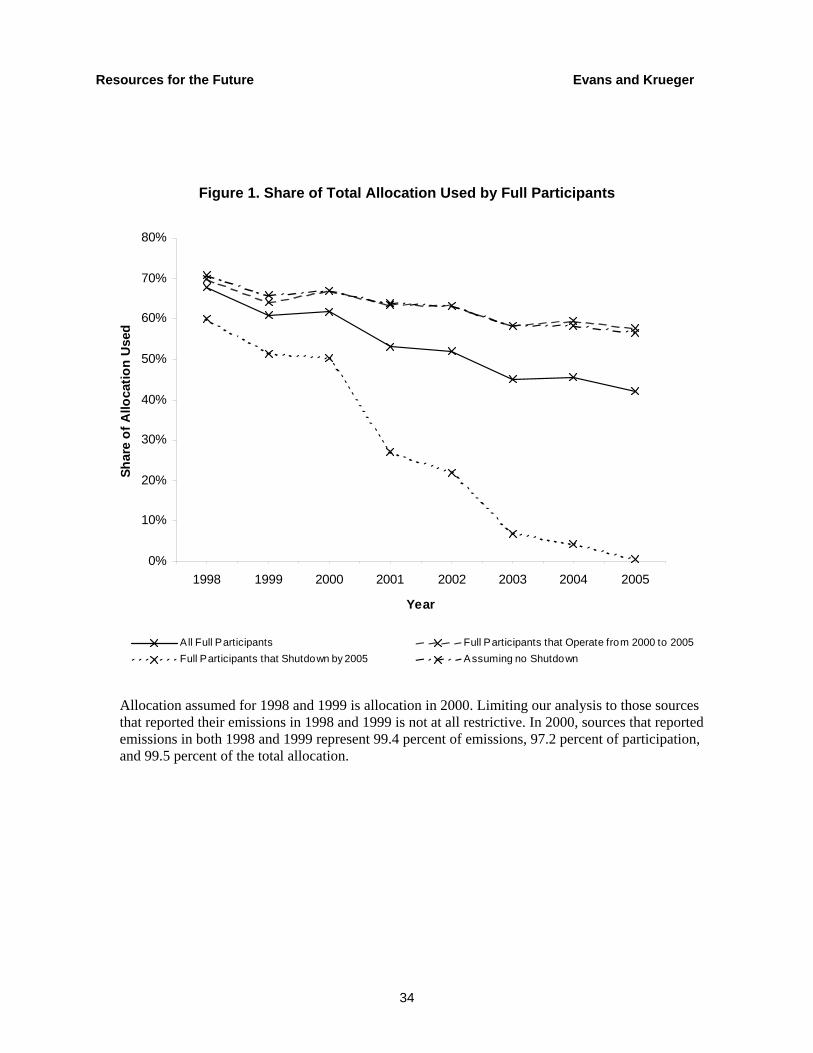
Resources for the Future Evans and Krueger
34
Figure 1. Share of Total Allocation Used by Full Participants
0%
10%
20%
30%
40%
50%
60%
70%
80%
1998 1999 2000 2001 2002 2003 2004 2005
Year
Shar
e of
Allo
catio
n U
sed
All Full Participants Full Participants that Operate from 2000 to 2005Full Participants that Shutdown by 2005 Assuming no Shutdown
Allocation assumed for 1998 and 1999 is allocation in 2000. Limiting our analysis to those sources that reported their emissions in 1998 and 1999 is not at all restrictive. In 2000, sources that reported emissions in both 1998 and 1999 represent 99.4 percent of emissions, 97.2 percent of participation, and 99.5 percent of the total allocation.
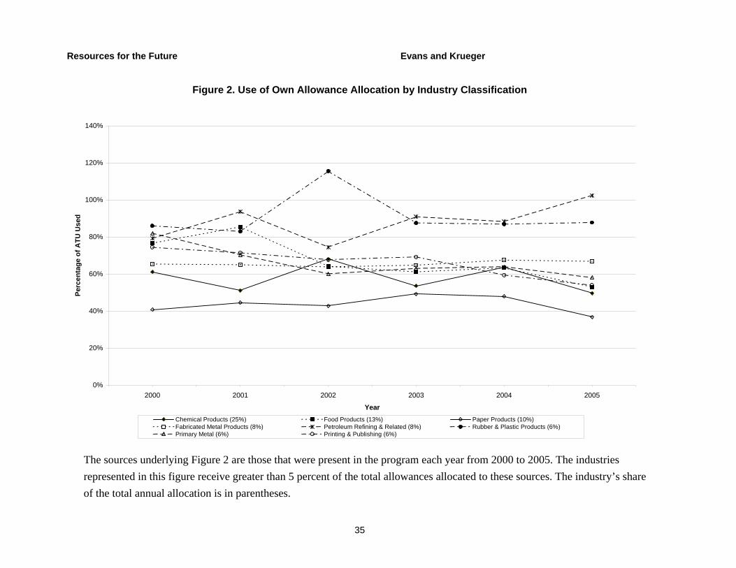
Resources for the Future Evans and Krueger
35
Figure 2. Use of Own Allowance Allocation by Industry Classification
0%
20%
40%
60%
80%
100%
120%
140%
2000 2001 2002 2003 2004 2005
Year
Perc
enta
ge o
f ATU
Use
d
Chemical Products (25%) Food Products (13%) Paper Products (10%)Fabricated Metal Products (8%) Petroleum Refining & Related (8%) Rubber & Plastic Products (6%)Primary Metal (6%) Printing & Publishing (6%)
The sources underlying Figure 2 are those that were present in the program each year from 2000 to 2005. The industries represented in this figure receive greater than 5 percent of the total allowances allocated to these sources. The industry’s share of the total annual allocation is in parentheses.

Resources for the Future Evans and Krueger
36
References
Ahman, M., D. Burtraw, J. Kruger, and L. Zetterberg. 2005. A Ten Year Rule to Guide the Allocation of EU Emissions Allowances, Clipore Report Series, No. 2005-1, August 2005.
Bluestein, J. 2003. Testimony of Joel Bluestein before the Committee on Environment and Public Works, Subcommittee on Clean Air, Climate Change and Nuclear Safety, United States Senate, May 8, 2003. http://epw.senate.gov/108th/Bluestein_050803.pdf (accessed April 1, 2006).
Burtraw, D., D.A. Evans, A. Krupnick, K. Palmer, and R. Toth. 2005. “Economics of Pollution Trading for SO2 and NOX.” Annual Review of Environment and Resources 30:253-289.
Burtraw, D. and D.A. Evans. 2004. “NOX Emissions in the United States: A Potpourri of Policies.” In Choosing Environmental Policy: Comparing Instruments and Outcomes in the United States and Europe. W. Harrington, R. Morgenstern, and T. Sterner, Eds. Washington, DC: Resources for the Future.
Council of State Governments. 2003. Innovative State Environmental and Natural Resource Programs. http://ssl.csg.org/innovations/2003/environment/2003envrpt.pdf (accessed February 15, 2006).
Ellerman, A.D., P. Joskow, R. Schmalensee, J.P. Montero, and E. Bailey. 2000. Markets for Clean Air, The U.S. Acid Rain Program. New York: Cambridge University Press.
European Commission. 2003. “Directive 2003/87/EC of the European Parliament and of the Council of 13 October 2003 establishing a scheme for greenhouse gas emission allowance trading within the Community and amending Council Directive 96/61/EC,” Official Journal of the European Union L 275/32, 25.10.2003.
European Commission . 2005. “Further guidance on allocation plans for the 2008 to 2012 trading period of the EU Emissions Trading Scheme,” COM (2005) 703 final, Brussels, 22.12.2005.
Evans, D.A. 1999. An Analysis of the Proposed Emissions Reduction Market System for Volatile Organic Materials in Chicago. Master’s thesis, Department of Agricultural and Consumer Economics, University of Illinois at Urbana-Champaign.
Resources for the Future Evans and Kruger
37
Federal Register. 2001. Approval and Promulgation of Implementation Plans; Illinois Trading Program 66(199):52343-52359.
Federal Register. 2005. Consumer and Commercial Products: Schedule for Regulation 70(221):69759-69761.
Foster, V. and R.W. Hahn. 1995. “Designing More Efficient Markets: Lessons form Los Angeles Smog Control.” Journal of Law and Economics 38:19-48.
Grubb, M. and K. Neuhoff, 2007. “Allocation and competitiveness in the EU Emissions Trading System: Policy Overview.” Climate Policy (forthcoming).
Hamilton, J.T. 2005. Regulation through Revelation: The Origin, Politics, and Impacts of the Toxics Release Inventory Program. New York: Cambridge University Press.
Harrison, D. 2004. “Ex Post Evaluation of the RECLAIM Emissions Trading Programmes for the Los Angeles Air Basin.” In Tradeable Permits: Policy Evaluation, Design and Reform. Paris: Organization for Economic Cooperation and Development.
Hepburn, C., M. Grubb, Neuhoff, K., Matthes, F., and M. Tse, 2007. “Auctioning of EU ETS Phase II allowances: How and why?” Climate Policy (forthcoming).
Henderson, V.J. 1996. “Effects of Air Quality Regulation.” The American Economic Review 86(4):789-813.
Illinois Environmental Protection Agency. 1995. Design For VOM Emissions Trading System. Author: Springfield, IL.
Illinois Environmental Protection Agency. 1996a. Emissions Reduction Market System Adoption of 35 Ill. Adm. Code 205 and Amendments to 35 Illinois Administrative Code 106: Statement of Reasons. Author: Springfield, IL.
Illinois Environmental Protection Agency. 1996b. Technical Support Document for VOM Emissions Reduction Market System. Author: Springfield, IL.
Illinois Environmental Protection Agency. 2001-2006. Annual Performance Review Report: Emissions Reduction Market System. http://www.epa.state.il.us/air/erms/apr/index.html (accessed May 1, 2006).
Jaffe, A. B., R.G. Newell, and R.N. Stavins. 2003. “Technological Change and the Environment.” In Handbook of Environmental Economics. Karl-Göran Mäler and Jeffrey Vincent, Eds. Amsterdam, The Netherlands: North-Holland/Elsevier Science.
Resources for the Future Evans and Kruger
38
Klier T.H., Mattoon R.H., and Prager M.A. 1997. “A mixed bag: assessment of market performance and firm trading behavior in the NOx RECLAIM Programme.” Journal of Environmental Planning and Management 40(6):751-74
Kling, C.L. and J. Zhao. 2000. “On the Long-Run Efficiency of Auctioned vs. Free Permits.” Economics Letters 69:235-238.
Kosobud, R.F., H.H. Stokes, C.D. Tallarico, and B.L. Scott. 2004. “The Chicago VOC Trading System: The Consequences of Market Design for Performance.” MIT CEEPR Working Paper WP-2004-019. http://web.mit.edu/ceepr/www/2004-019.pdf (accessed March 13, 2005).
Kruger, J.A. and W.A. Pizer. 2004. “Greenhouse gas trading in Europe: The new grand policy experiment.” Environment 46(8):8-23.
Lents, J.M. 2000. “The RECLAIM Program (Los Angeles’ Market-Based Emissions Reduction Program) at Three Years.” In Emissions Trading: Environmental Policy's New Approach. R.F. Kosobud, D.L. Schreder, H.M. Biggs, Eds. New York, New York: National Association of Manufacturers.
Magat, W.J., A.J. Krupnick and W. Harrington. 1986. Rules in the Making : A Statistical Analysis of Regulatory Agency Behavior. Washington, DC: Resources for the Future.
McLean, B.J. 1997. “Evolution of marketable permits: The U.S. experience with sulfur dioxide trading.” International Journal of Environment and Pollution 8(1/2):19–36.
Montero, J.P., J.M. Sanchez and R. Katz, 2002. “A Market-Based Environmental Policy Experiment in Chile.” Journal of Law and Economics Vol. XLV, April.
National Commission on Energy Policy (NCEP). 2004. Ending the Energy Stalemate: A Bipartisan Strategy to Address America's Energy Challenges. Washington, DC: National Commission on Energy Policy.
Palmer, K., W. E. Oates and P.R. Portney. 1995. “Tightening Environmental Standards: The Benefit-Cost or the No-Cost Paradigm?” The Journal of Economic Perspectives 9(4):119-132.
Pizer, W.A. 2002. “Combining Price and Quantity Controls to Mitigate Global Climate Change.” Journal of Public Economics 85(3):409-434.
Point Carbon, 2006. Carbon Market Europe, May 12, 2006.
Resources for the Future Evans and Kruger
39
Porter, M.E. and C. van der Linde. 1995. “Toward a New Conception of the Environment-Competitiveness Relationship” The Journal of Economic Perspectives 9(4):97-118.
Regional Greenhouse Gas Initiative. 2005. “Memorandum of Understanding,” accessed at http://www.rggi.org/docs/mou_12_20_05.pdf (accessed January 10, 2006)
Solomon, B.D. and H.S. Gorman. 1998. “State-Level Air Emissions Trading: The Michigan and Illinois Models.” The Journal of Air and Waste Management 48:1156-1165.
Sterner, T. 2003. Policy Instruments for Environmental and Natural Resource Management. Washington, DC: Resources for the Future.
Thompson, D.B. 2000. “Political Obstacles to the Implementation of Emissions Markets: Lessons from RECLAIM.” Natural Resources Journal 40(3):645-697.
Tripp, J.T.B. and D. J. Dudek. 1989. “Institutional Guidelines for Successful Transferable Rights Programs.” Yale Journal of Regulation 6:369-90.
U.S. Environmental Protection Agency. 2000. Taking the Toxics Out of the Air. EPA-452/K-00-002. http://www.epa.gov/oar/oaqps/takingtoxics/airtox.pdf (accessed March 23, 2006).
U.S. Environmental Protection Agency. 2006. Table of Final MACT Rules. http://www.epa.gov/ttn/atw/mactfnl.html (accessed March 30, 2006).
Weil, D., A. Fung, M. Graham, and E. Fagotto. 2006. “The Effectiveness of Regulatory Disclosure Policies.” Journal of Policy Analysis and Management 25(1):155–181.