Distribution Category:Mathematics and Computers

(UC-32)

ANL-82-45

ArJL--82-45

DE83 003342

ARGONNE NATIONAL LABORATORY9700 South Cass Avenue

Argonne, Illinois 60439

A METHODOLOGY FOR ALGORITHM DEVELOPMENTTHROUGH SCHEMA TRANSFORMATIONS

by

M. N. Muralidharan

Mathematics and Computer Science Division

July 192

Based on a thesis prepared forthe degree of Doctor of Philosophy

for the Indian Institute of Technology, Kanpur

3

TABLE OF CONTENTS

Page

LIST OF SYMBOLS........................................................ 6

ABSTRACT....................... ....... ......................... ... 7

CHAPTER 1 INTRODUCTION............................................. 9

1.1 Scope of the Report .................... 9

1.2 Organization of the Report........................... 9

CHAPTER 2 LITERATURE SURVEY......................................... 11

2.1 Program Synthesis Systems............................ 11

2.2 Program Manipulating systems......................... 14

2.3 Programming Languages and Techniques................. 16

2.4 Discussion and Present Work.......................... 16

CHAPTER 3 OUTLINE OF THE METHODOLOGY................................. 18

3.1 Basic Notations and Rues......u...................... 18

3.2 Multiple Refinement.................................. 29

CHAPTER 4 DERIVATION OF PERMUTATION GENERATION ALGORITHMS........... 32

4,1 Recursive Permutation Algorithms..................... 32

4.2 Relation to the Work of Darlington and of

Sedgewick............................................ 53

CHAPTER 5 RELATED PROBLEMS... .... ................................... 56

5.1 Stack Permutations and Tree Codes.................... 565.2 An Algorithm for Generating Stack Permutations....... 585.3 Correspondence between Stack Permutations and

Tree Codes ........................................... 62

CHAPTER 6 CONCLUSION................................................ 68

ACKNOWLEDGMENTS ........................................................ 69

REFERENCES ............................................................. 70

APPENDIXES

A. Listing of the Permutation Algorithms........................... 73

B. Implementation of the Permutation Algorithm in LISP............ 76

4

LIST OF FIGURES

No. Title Pag

4.1 Representation of a permutation 'ABCD' as a bijective function.... 32

4.2 The structure of the derivation................................... 34

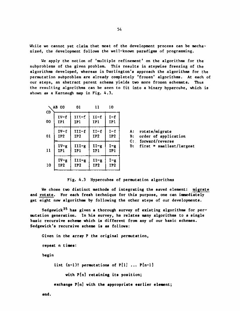
4.3 Hypercubes of permutation algorithms.............................. 54

5.1 Labelling a binary tree........................................... 57

5.2 All possible binary trees with 3 internal nodes................... 59

5.3 A binary tree with node numbers................................... 62

5.4 Tree for rule 2 ................................. 65

5.5 Tree for rule 3................................................ ... 65

5

LIST Of STIBO.

6

Symbol

C

0

U

n

x

3

[]e

O

0u

underline

+

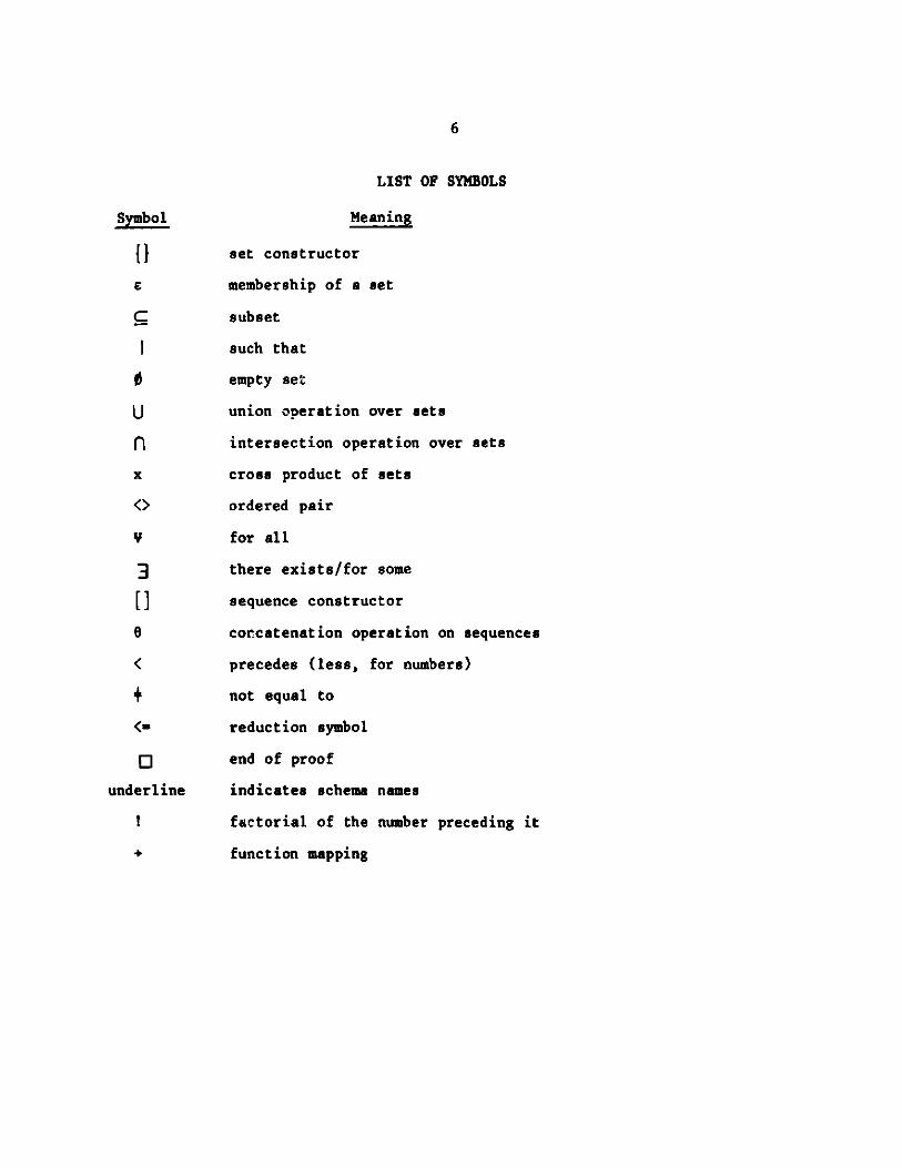
LIST OF SYMBOLS

Meaning

set constructor

membership of a set

subset

such that

empty set

union operation over sets

intersection operation over sets

cross product of sets

ordered pair

for all

there exists/for some

sequence constructor

concatenation operation on sequences

precedes (less, for numbers)

not equal to

reduction symbol

end of proof

indicates schema names

factorial of the number preceding it

function mapping

7

A METHODOLOGY FOR ALGORITHM DEVELOPMENTTHROUGH SCHEMA TRANSFORMATIONS

by

M. N. Muralidharan

ABSTRACT

A programming methodology based on schema transformations

is presented. Such an approach is a logical outcome of recentdevelopments in program manipulating systems. Concurrent

development of algorithms and their proofs of correctness is a

significant feature of the proposed methodology. As the

development process begins with an abstract schema, it is

often possible to derive several related end algorithms in a

single development process. This has implications in both the

economics of software development and the understanding and

teaching of algorithms.

The initial schematic specification (a skeleton algorithm

schema), the intermediate and final algorithm schemata are all

expressed in Darlington's first-order recursion equation

language exploiting set-theoretic constructs. A set of trans-

formation rules together with a set of reduction rules for set

expressions is then used to successively transform the sche-

matic specification into different algorithm schemata. Most

of the transformations are applications of a small number of

common rewriting rules.

Combinatorial problems are chosen for their simplicity

and elegance, which allows us to keep the illustrations brief.

However, the methodology can be applied to other domains once

appropriate systems of transformations are defined in these

domains. Three problems are considered: 1) generating all

permutations of a set of objects, 2) generating stack permuta-tions, and 3) generating all binary trees with n nodes. We

conclude by discussing the problems that need further investi-gations and suggesting directions for further work.

8

9

CHAPTER 1

INTRODUCTION

1.1 Scope of the Report

This report is concerned with the problem of developing a methodology for

simultaneously deriving several algorithms for a given problem. The techniqueproduces proofs of the algorithms as a natural by-product of algorithm devel-opment. Such a methodology promises to make program development more reli-

able. Further, since a battery of different solutions becomes available, onecan be adaptive to the envirorL:ent of the problem by choosing the most appro-

priate one for each occasion.

The methodology presented here is based on schema transformations. We

start with an abstract schema based on the problem definition and then, by

using a set of transformation rules together with a set of reduction rules forset expressions, successively transform the abstract schema into a set ofalgorithm schemata. We apply the notion of 'multiple refinement' to the de-

velopment of algorithms for the subproblems of a given problem.

Most of the transformations are applications of a small number of rewrit-

ing rules. As the development process begins with an abstract schema, it is

often possible to derive several related end algorithms in a single develop-ment process. There are two noteworthy features of the methodology:

1. Once the initial schematic specification and the transformationsused are shown correct, correctness is preserved at each step of the

derivation process.

2. Schematic specification and subsequent derivation of the algorithmschemata make it possible to derive several algorithmssimultaneously.

The methodology is illustrated by deriving algorithms for a combinatorialproblem and later adapting the development for variants of the problem. Thenatural simplicity and elegance of combinatorics allow us to keep the illus-trations brief. However, there is nothing in our methodology which is inher-ently restricted to a specific problem domain. The methodology can be appliedto other domains once appropriate systems of transformation are establishedfor the domain concerned.

1.2 Organisation of the Report

In Chapter 2, we give a survey of the literature relevant to our work.The areas touched upon include program synthesis systems, program manipulatingsystems, and programming languages and techniques. We describe a few inter-esting systems in each of these areas and then conclude the survey by a dis-cussion of these systems in the context of our work.

10

Chapter 3 outlines the main features of the methodology for algorithm

development proposed in the paper. Basic notations and rules used are de-

scribed, by giving examples wherever necessary, followed by a description of

the notion of 'multiple refinement' used in the methodology.

In Chapter 4, we apply the methodology to the problem of generating allpermutations of the elements of a given set. A set of sixteen variantalgor' thins for permutation generation is derived. In the last part of thechapter we discuss the relation with Darlington's work9 and Sedgewick'swork.35

In Chapter 5, one algorithm from the previous chapter is adapted forhandling a related problem of generating stack permutations. We firstanalyze properties of stack permutations to arrive at a test that can be usedin conjunction with the given permutation algorithm. This test is thenintegrated into that algorithm to achieve the desired result. Then, we

establish a correspondence between stack permutations and binary trees. Thiscorrespondence can be utilized for generating all binary trees with a given

number of nodes.

In the final chapter, we give our conclusions and suggest possibledirections for future research.

11

CHAPTER 2

LITERATURE SURVEY

The growing need for developing reliable programs has necessitated the

invention of new tools for program development. It is well known that the

human input is the major component in software development. This fact has led

some peopLe to develop new prOgramming languages and systems that reduce thetotal amount of human input needed and systematize whatever human contribution

is essential. These systems occupy a wide spectrum, ranging from fully auto-

matic systems to completely manual systems. In this chapter, we have at-

tempted to sample systems from that spectrum.

There are program synthesis systems that allow the user to specify theintent of his program in a suitable specification language and then construct

automatically a (correct) program meeting the given specification. In these

systems, the human involvement is minimal.

Then, there are systems that accept a rough-hewn source program in a highlevel language (possibly a very inefficient one) and produce a polished ver-

sion of it by way of program manipulation. Here the human involvement is ingiving a correct source program initially and further guiding the system in

developing the desired efficient program. Preservation of correctness with

each manipulation applied to the source program is guaranteed by the system.

In these systems, which could be called 'computer-aided,' the amount of human

involvement is somewhat more than in program synthesis systems.

On the other end of the spectrum there are languages supporting a par-

ticular programming discipline that is known to increase reliability of the

programs developed. These languages offer abstraction facilities so that theuser can clearly and correctly express the problem by choosing abstractions

appropriate to his problem domain. Compilers are then equipped with facili-ties for checking the user-supplied assertions.

The following sections contain a survey of the system mentioned above.

2.1 Program Synthesis Systems

Program synthesis systems enable the user to specify the intent of his

program by giving input-output predicates (as in the DEDALUS system33) ortraces7 or natural language (the SAFE system2'3) or a mixture of all of

these (the PSI program synthesis system 1 5, 1 6 ) and then automatically synthe-sizes the required program. Biermann7 gives a survey of automatic programsynthesis systems. Considerable progress has been made in the implementationof DEDALUS and PSI systems, and we describe here the important characteristics

of these two systems.

12

2.1.1 The DEDALUS System

Manna's approach to automatic program synthesis has evolved out of his

earlier work in the area of program verification (see Ref. 32). His systemDEDALUS applies deductive techniques to systematically derive programs from

given specifications. The control structure of the synthesized programs isdeveloped by using deduction in the derivation process.

The system takes a program specified as input-output predicates and suc-

cessively transforms the nonprimitive constructs in the specification into

primitive constructs in the LISP-like target language. In the process, con-ditionals and recursive calls are introduced as and when their need is recog-

nized by the deductive system. Simultaneously with the creation of theprogram, the system develops a proof of total correctness of the program. The

domain of the programs constructed consists of sets (and lists) of integers.

.The system employs a large number of transformation rules. It repeatedlyapplies these rules to the given specification until a program containing only

primitive constructs is produced. Some transformation rules exploit proper-

ties of the underlying domains (i.e., properties of integers or list struc-

tures). Other rules are based on the meaning of the constructs in thespecification and target languages (e.g., head(1) in the target language).Finally, there are rules that represent a formulation of basic programmingtechnique which do not depend on a particular subject domain (e.g., the intro-

duction of conditional expressions and recursion).

The system uses deduction in two situations:

1. In cases where the conditions associated with the rules cannot be

applied unless the conditions have been proven correct in the

current context.

2. In cases where the conditions have not been proven, for introducing

conditional control structure in order to provide contexts in which

the conditions are provable (and hence the rule can be applied).

The system is implemented in QLISP, a language having pattern-matchingand backtracking facilities. The specifications are expressed in a languagesupporting very high-level constructs from the subject domain of the applica-

tion. The synthesized program are in a language close to LISP. The trans-formation rules are expressed as programs in the QLISP language. The systemcontains more than a hundred transformation rules. The programs successfullyconstructed by the system include those for finding the maximum element of alist of integers, greatest co..on divisor of two integers, and artesianproduct of two sets.

13

2.1.2 The PSI Program Synthesis System

The PSI program synthesis project, started under the guidance of

Green,15 ,16 has the design goal of developing a system that would accept high-level descriptions of program as specification and synthesize a program out of

it. As of last report available, only one module of the system is ready. Thefollowing discussion describes the design.

The user specifies the desired program in natural language, input-outputpairs and partial traces. Then, the system synthesizes the programs in a

LISP-like language. In the process of synthesis, interactive dialogues be-

tween the user and the system may occur, where each is to take the initiative

in leading the discussion and asking questions as the situation demands.

This system has a large knowledge-base containing a great deal of informa-

tion about the domains of programs and certain programming principles, as well

as information necessary for discussing a program with the user. According to

the design of the system, it is to be organized as a collection of closelyinteracting modules or experts. The modules proposed in the design are listed

below:

1. Parser Interpreter

The parser-interpreter module has the function to parse and par-

tially interpret sentences into less linguistic and more program-oriented

terms.

2. Trace Expert

The trace expert infers program model fragments from the given input

traces and sends them to the model builder.

3. Discourse Expert

The discourse expert models the user, the dialogue, and the state of

the system and then uses these models to select appropriate questions or

statements to present to the user.

4. Domain Expert

The domain expert takes as input the partially interpreted sentencesfrom the natural language expert and produces fragments of program descriptionin a program description-oriented language called FRAGMENTS, to be given tothe model builder to assemble.

14

5. Model Building Expert

The model building expert takes as input the fragments of programdescription from domain expert cr trace expert and produces a complete algo-

rithm and information structure model.

6. Coding Expert

The coding expert takes the program model from the model expert andproduces code in target language. It interacts closely with the efficiency

expert in this task.

7. Efficiency Expert

The efficiency expert selects efficient algorithms and data struc-

tures from the alternatives offered by the coding expert.

Of the module's stated above, the implementation of only the coding mod-ule, called PECOS, has been reported in the literature as completed.4 ,5 ,1 7

The status of implementation of other modules is not known.

The code expert, PECOS, takes an abstract description of a program and

successively refines this description by applying rules until a concrete

executable program in LISP is produced. The knowledge-base of PECOS contains

about 400 rules. PECOS interacts with the user or efficiency expert (as

required by the situation) in producing the code.

2.2 Program Manipulating Systems

The systems described in the previous section aimed at synthesizing aprogram in a high-level language, given the specification of the program,whereas the program manipulating systems, to be described now, take as input a

source program in a high-level language and modify it in order to improve its

efficiency, by applying source-to-source transformations to it.

Source-to-source transformation techniques have evolved from the work on

developing systems that improved the execution time of the object code pro-

duced by a compiler by applying a set of optimizing transformations like con-

stant folding, invariant code ,vement, and common subexpression elimination.1

In these systems, once the object code is generated, optimization of theobject code is done by applying optimizing transformations automatically; the

process of optimization is neither visible nor explicitly accessible to the

user. It was found that if manipulations are carried out at the source

language level instead of at object code level, it is possible for the user todevelop efficient programs. The system will automatically produce an effi-cient program starting with an inefficient one, by choosing and applyingappropriate program transformations.6 ,8,10 ,18,19, 3 1 ,34 ,38 ,4 0 The basic

15

philosophy in all these systems is that a catalogue of transformations isstored in the system; and given a program, the system will successively trans-

form it into another which may be an improvement over the first.

We now describe two of the successfully implemented source-to-source

transformation systems.

2.2.1 Burstall and Darlington's System

The Burstall and Darlington's system allows the user to specify the pro-gram in the form of a set of equations in a first-order recursion equation

language called NPL. The system then modifies the given set of equations intoa new set by applying transformation rules--namely, definition, instantiation,

unfolding, folding and rules based on domain properties. The user must guide

the evolution of the program through the system. The system carries each lead

given by the user to its conclusion, making as many transformations as possi-

ble and leaving it to the user to judge the outcome.

Their initial system10 removed recursion in favor of iteration from theprogram given in the form of recursion equations. It was extended later,8 so

that it allows more manipulations to be made before removing recursion. Thus,the extended system transforms a recursive program into another recursive one

by a sequence of manipulations, before ultimately converting them into a pro-

gram in a procedural language. This kind of source-to-source manipulation is

shown to yield better improvements to the program than the first system. This

fact was illustrated by the authors by deriving efficient programs for finding

fibonacci number, for computing the table of factorials, and for computing the

sums and products of 'tips' of a tree.

The final programs produced by the system are in LISP. The current

implementation, as reported in Ref. 8, requires the user to give the following:

1. A list of equations augmented by any new definitions ('eureka'

definitions).

2. A list of useful lemmas in equational form (for use as rewriterules) and statements of which functions are associative or commutative or

both.

3. A list of all the properly instantiated left-hand sides of the equa-tions on which the user wants the system to work. The system then modifiesthe given equations by applying the transformation rules. The resulting newequations are printed out for examination by the user.

2.2.2 SPECIALIST

SPECIALIST is a prototype transformation system implemented at the

University of California at Irvine by Standish and his group. 23,38 It is a

16

pattern-directed source-to-source transformation system. A pattern-directedsystem is one that replaces a matched left-hand pattern with an instantiated

right-hand pattern. The transformations in the system do not change the basicstrategy of the algorithm. The system accepts Algol-like program as input and

applies a set of pattern-directed transformations automatically in order to

successively transform the program. It allows the user to specify the con-

straint or restriction on the data structure along with the input. The system

then attempts to simplify the input program to take advantage of the special-

ized data structure.

The system is implemented in LISP. It is a rule-based system containing

about fifty rules. A majority of the rules are language-independent. The

domain of the programs handled by the system is that of matrix computations.

2.3 Programing Languages and Techniques

Structured programing, as advocated by Dijkstra,1 2 Knuth,2 7 and

Wirth,4 1 ,42,43 involves systematic use of abstraction in program development.In such an approach, the program development goes through different levels of

abstraction, from the most abstract program at the topmost level, throughlesser and lesser abstract programs in successive levels, to a level where the

program is fully in concrete form. The goal is to develop programs in a

systematic manner so that it is simpler to reason about and easier to under-

stand them. This initiated development of new programming languages support-

ing this philosophy.

Since a program consists of a data structure part and a control structure

part, abstraction of each is possible. Therefore, new languages supporting

data abstraction (CLU, 2 9 , 3 0 ALPHARD,3 6 ,4 4 EUCLID2 8) and control abstraction14

have been developed in the recent years. Apart from offering abstraction

facilities, these languages have constructs specifically designed to aid in

the verification of programs written in them. The verification techniques

used in these languages are based on the invariant assertion method pioneered

by Floyd,1 3 and developed by Hoare,2 0-2 2 and others. Other verification

styles have been proposed elsewhere.1 1

2.4 Discussion and Present Work

Program synthesis systems and program manipulating systems have theoreti-

cal as well as practical limitations. Theoretically, it is known that these

systems are not complete. That is, given any system, one can always find

programing problems whose solutions will necessitate adding more rules to thesystem. On the practical side, storage and time are the limiting factors. Alarge number of rules need to be stored and constantly searched for possibleapplication. 'Intermediate swell' of the problem also strains storage. Thealgorithms for rule application are time-consuming.

17

In DEDALUS, the process of introducing conditional expressions may become

somewhat time-consuming, as it involves exhausting all the rules that mightapply to each condition that could not be proved or disproved. A certain

amount of futile theorem-proving effort is always expended in situations whereone can neither prove or disprove the condition. At any stage of the synthe-

sis, if the specifications are too general, DEDALUS may not be able to con-

struct a program. According to the report, 33 there is no way in which thesystem can avoid such situations. Efficiency is not considered while synthe-

sizing a program. Programs constructed by the system may be very inefficient.

The system is restricted to the construction of programs involving lists and

simple arrays only. Certain classes of programs (e.g., operating systems)cannot be described by input-output relationship, and there is no way in which

such programs can be specified to the system.

The PSI program synthesis system has been able to successfully construe t

sort, set union and other programs. It has programming knowledge for space

reutilization, ordered set enumeration, and divide-and-conquer paradigm. The

knowledge is represented as rules in the system; there are about 400 rules

included.1 7 Not all the rules have been implemented, nor is the system fully

implemented.

Burstall and Darlington's system does only the routine rewriting task on

a given set of equations and leaves it to the user to guide the evolution of

the desired program.8 The system is not interactive. The user and the systemwork independently in the evolution process. The system does not assess the

efficiency of the program developed.

In SPECIALIST, many optimizations require a deeper understanding of the

algorithm's intent than the source code level of representation it provides.

Strict pattern-directed behavior of the system may obscure certain simplifica-

tions which would otherwise be possible if manipulations of the pattern wereallowed.

The programming languages supporting data abstraction and control ab-

straction require the user to supply the relevant invariant assertions of hisprograms so that the correctness can be machine-checked. It is not always

easy to find the invariant assertions, and therefore it is an additional

burden on the user to supply them.

In all the systems described so far, there is little or no scope fortrying out new methods or techniques, whereas in manual systems, one can try

out new ideas and techniques. We present a novel methodology for deriving a

set of algorithms, starting from the problem definition and applying programtransformation techniques. Simultaneously with the development of algorithms,

we develop their proofs also. Though the methodology described involvesmanual development of algorithm, certain steps in the development lend them-selves to automation on the lines of the program manipulating system. 8 ,37 ,38

18

CHAPTER 3

OUTLINE OF THE METHODOLOGY

In this chapter, we develop our methodology for program development byderiving a set of algorithms for a small problem. Basic notations and rules

used are explained first. The correctness of the rules is shown next, and

finally the methodology is illustrated by means of a small example.

3.1 Basic Notations and Rules

We use the equational notation of the first-order recursion equation

language proposed by Burstall8'9 for specifying the algorithm and employ

transformation rules and set-reduction rules as explained therein. For the

sake of completeness, we explain below the basic notations and rules, withillustrations wherever necessary.

3.1.1 Notation

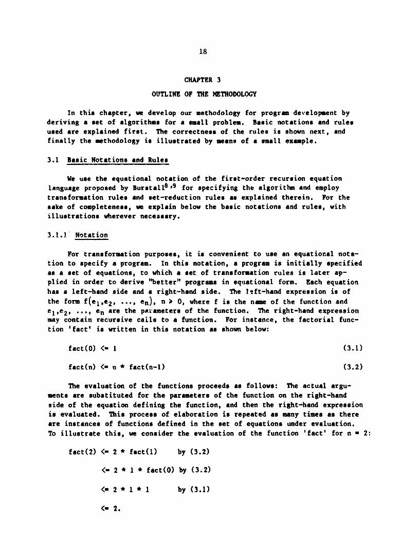
For transformation purposes, it is convenient to use an equational nota-

tion to specify a program. In this notation, a program is initially specifiedas a set of equations, to which a set of transformation rules is later ap-plied in order to derive "better" programs in equational form. Each equationhas a left-hand side and a right-hand side. The left-hand expression is ofthe form f(e1,e2 , ... , en), n > 0, where f is the name of the function andei,e2 , ... , en are the parameters of the function. The right-hand expressionmay contain recursive calls to a function. For instance, the factorial func-

tion 'fact' is written in this notation as shown below:

fact(0) <= 1 (3.1)

fact(n) <= n * fact(n-1) (3.2)

The evaluation of the functions proceeds as follows: The actual argu-

ments are substituted for the parameters of the function on the right-hand

side of the equation defining the function, and then the right-hand expression

is evaluated. This process of elaboration is repeated as many times as there

are instances of functions defined in the set of equations under evaluation.

To illustrate this, we consider the evaluation of the function 'fact' for n - 2:

fact(2) <= 2 * fact(1) by (3.2)

<= 2 * 1 * fact(O) by (3.2)

<= 2 * 1 * 1 by (3.1)

< 2.

19

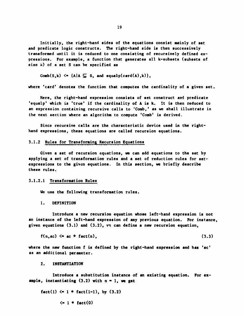
Initially, the right-hand sides of the equations consist mainly of setand predicate logic constructs. The right-hand side is then successivelytransformed until it is reduced to one consisting of recursively defined ex-

pressions. For example, a function that generates all k-subsets (subsets of

size k) of a set S can be specified as

Comb(S,k) <= (A|A S, and equalp(card(A),k)},

where 'card' denotes the function that computes the cardinality of a given set.

Here, the right-hand expression consists of set construct and predicate

'equalp' which is 'true' if the cardinality of A is k. It is then reduced toan expression containing recursive calls to 'Comb,' as we shall illustrate in

the next section where an algorithm to compute 'Comb' is derived.

Since recursive calls are the characteristic device used in the right-hand expressions, these equations are called recursion equations.

3.1.2 Rules for Transforming Recursion Equations

Given a set of recursion equations, we can add equations to the set byapplying a set of transformation rules and a set of reduction rules for set-

expressions to the given equations. In this section, we briefly describe

these rules.

3.1.2.1 Transformation Rules

We use the following transformation rules.

1. DEFINITION

Introduce a new recursion equation whose left-hand expression is notan instance of the left-hand expression of any previous equation. For instance,

given equations (3.1) and (3.2), v- can define a new recursion equation,

f(n,ac) <" ac * fact(n), (3.3)

where the new function f is defined by the right-hand expression and has 'ac'as an additional parameter.

2. INSTANTIATION

Introduce a substitution instance of an existing equation. For ex-

ample, instantiating (3.2) with n - 1, we get

fact(1) <a 1 * fact(1-1), by (3.2)

<- 1 * fact(o)

20

<= 1 * 1, simplifying with (3.1)

<= 1.

3. UNFOLDING

If E <= F and G < H are equations and there is an occurrence in H of

a symbolic instance of E, then G <- H can be rewritten as G <= I, where I is

obtained by replacing every occurrence of the symbolic instance of E by the

corresponding symbolic instance of F. For example, given equations (3.1),

(3.2) and (3.3), let us apply the unfolding rule to (3.3). We get

f(n,ac) <= ac * n * fact(n-1) (3.4)

** unfolding with (3.2).

4. DOMAIN PROPERTIES

We may transform an equation by using on its right-hand expression

any laws we have about the primitives used therein, obtaining a new equation.

For instance, equation (3.4) can be simplified as

f(n,ac) <_ (ac * n) * fect(n-1) (3.5)

** by associative property of multiplication.

5. FOLDING

If E <= F and G <= H are equations and there is an occurrence in Hof a symbolic instance of F, then G <= H can be rewritten as G <= I, where Iis obtained by replacing every symbolic occurrence of F in H by the corre-sponding symbolic instance of E. For example, (3.5) can be rewritten as

f(n,ac) <= f(n-1, ac * n)

** folding with (3.3).

The unfolding rule above corresponds to the symbolic evaluation of

recursively defined functions. Folding is the rule by means of which recur-

sions are introduced into a system of equations.

Now, we illustrate the application of all these rules by a set of

examples.

Example 1:

Find the sum of a set of integers, S,

sum(0) <= 0, given, (3.6)

sum(S) <0 one(S) + sum(rest(S,one(S))), given. (3.7)

21

The function 'one' returns an element of the set S, and the function 'rest'returns all the elements of S except one(S).

Let us define 'f' as follows:

f(rest(S,one(S)),ac) <= ac + sum(rest(Sone(S))) (3.8)

** definition (eureka)

f(0,ac) <= ac + sum(o), instantiating (3.8)

<= ac + 0, using (3.6)

<= ac (3.9)

f(S,ac) <= ac + sum(S), instantiating (3.8)

<= ac + one(S) + sum(rest(S,one(S)))

** unfolding with (3.7)

<_ (ac + one(S)) + sum(rest(S,one(S)))

** by associative property of +

<= f(rest(S,one(S)), ac + one(S)) (3.10)

** folding with (3.8)

sum(S) <= f(rest(S,one(S)), one(S)) (3.11)

** folding (3.7) with (3.8).

Now, the new definition of 'sum' is

sum(o) <= 0

sum(S) <= f(rest(S, one(S)), one(S))

f(0,ac) <= ac

f(8,ac) <= f(rest(S,one(S)),ac+one(S)).

Example 2:

Given a program to compute the non-repetitive union of two sequences,write a program to compute the non-repetitive union of three sequences.

22

Let us assume that we are given a function 'union2' that takes twosequences (each one containing distinct elements) as arguments and returns asingle sequence c4 staining distinct elements:

union2(0,Y) <- Y (3.12)

(3.13 )union2(X,Y) <= union2(rest(X),Y),

if uccursp(first(X) ,Y)

<" [first(X)J e union2(rest(X),Y), otherwise.

The predicate occursp(a,S) returns 'true' if the element 'a' occurs in thesequence S, and 'false' otherwise.

Let 'union3' denote the function that computes the non-repetitiveunion.of three sequences. Given a definition of function 'union3,' we willfind a redefinition for it by applying transformation rules:

union3(X,Y,Z) <= union2(union2(X,Y),Z),given

union3(0,Y,Z) <= union2(union2(0,Y),Z),inst.

(3.14)

(3.14)

(3.15)<= union2(Y,Z)

** on simplification using (3.12).

Unfolding (3.14) with (3.13), we get

union3(X,Y,Z) <= union2(union2(rest(X),Y),Z) (3.16a)

if occursp(first(X),Y)

<- union2((firast(X)l e

union2(rest(X),Y),Z), otherwise. (3.16b)

Let W - [first(X)J

union2(rest(X),Y).

that W is also not

o union2(rest(X),Y). Then, first(W) " first(X), rest(W) -

In the context of (3.16a) and (3.16b), X not null impliesnull. Therefore, (3.16b) can be rewritten as

< union2(W,Z).

Further unfolding with (3.11) and simplifying with the definition of W, we get

<= union2(union2(rest(X),Y),Z),

if occursp(first(X),Z)

23

<_ [first(X)] union2(union2(resto.,,Y),Z),

otherwise. (3.16b1)

Upon folding (3.16a), (3.16b1) with (3.14), we get

union3(X,Y,Z) <= union3(rest(X),Y,Z)

if occursp(first(X),Y)

<= union3(rest(X),Y,Z)

if occursp(first(X),Z)

< [first(X)] 0 union3(rest(X),Y,Z), otherwise. (3.17)

Thus, -the new definition of 'union3' (the function computing the nonrepetitive

union of three sequences) is

union3(0,Y,Z) <= union2(Y,Z)

union3(X,Y,Z) <= union3(rest(X),Y,Z),

if occursp(first(X) ,Y)

<= union3(rest(X),Y,Z),

if occursp(first(X),Z)

<_ [first(X)] 0 union3(rest(X),Y,Z), otherwise.

3.1.2.2 Reduction Rules for Set-Expressions

We first describe the reduction rules for set-expressions, illustrating

their application by a set of examples, and then show their correctness.

Reduction Rules. In the case where we have set constructs on the right-

hand side of the equations that cannot be expanded further using program

transformation rules, we use the following set-reduction rules. The form of

the rule is

set-expression <= set-expression,

indicating that the expression on the left-hand side can be reduced to theexpression on the right.

24

1.

MR1:

MR2:

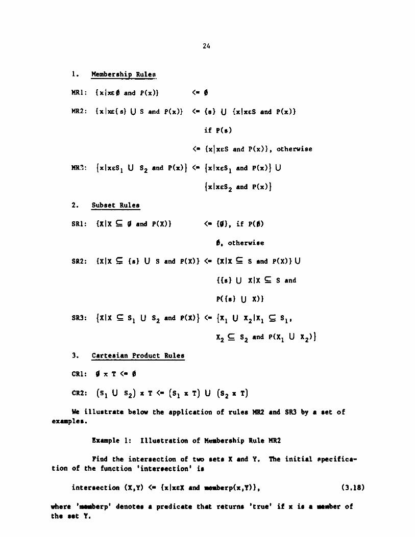
Membership Rulers

{xixc0 and P(x)}

{xaxe{s} U S and P(x)}

MRS: txixcSi U S2 and P(x)}

2.

SRI:

Subset Rules

(Xix C 0 and P(X)}

SR2: (XIX {s} U S and P(X)}

3R3: {XiX Si U S2 and P(X)}

3. Cartesian Product Rules

CR1: xT<=0

CR2: (SI U S2) x T <- (Si x T)

We illustrate below the applicatexamples.

0

(s) U {xixcS and P(x)}

if P(s)

{xlxeS and P(x)}, otherwise

{xixeS1 and P(x)} U

{xixeS2 and P(x)}

<= (0), if P(O)

0, otherwise

<' (xix R S and P(X)) U

{{s} U Xix 5 S and

P({s} U X)}

<= {X1 U X2 |i ElCS1,

X2 S2 and P(X1 U x2 )

U

ion

I

(s2 x T)

of rules MR2 and SR3 by a set of

Example 1: Illustration of Membership Rule MR2

Find the intersection of two sets X and Y. The initial specifica-tion of the function 'intersection' is

intersection (X,Y) <" (xixcX and memberp(x,Y)), (3.18)

where 'aemberp' denotes a predicate that returns 'true' if x is a member ofthe set Y.

25

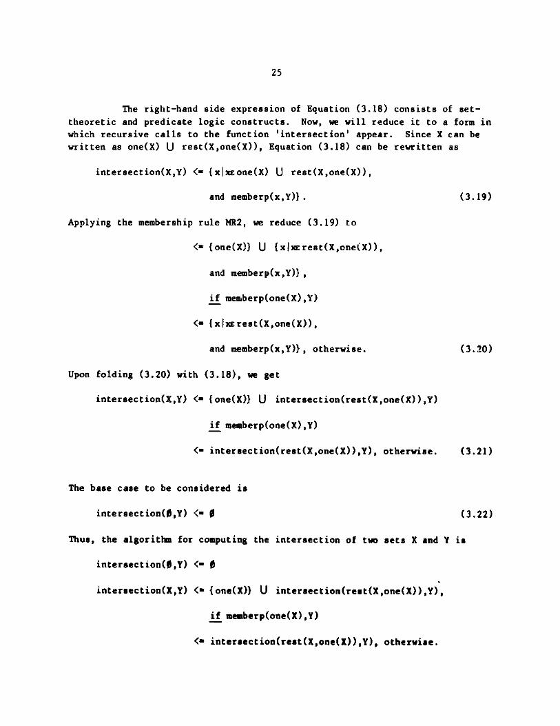
The right-hand side expression of Equation (3.18) consists of set-

theoretic and predicate logic constructs. Now, we will reduce it to a form inwhich recursive calls to the function 'intersection' appear. Since X can bewritten as one(X) U rest(X,one(X)), Equation (3.18) can be rewritten as

intersection(X,Y) < {xlxcone(X) U rest(X,one(X)),

and memberp(x,Y)). (3.19)

Applying the membership rule MR2, we reduce (3.19) to

<_ (one(X)) U (xlxErest(X,one(X)),

and memberp(x,Y)},

if memberp(one(X),Y)

<_ {xlxrest(X,one(X)),

and memberp(x,Y)}, otherwise. (3.20)

Upon folding (3.20) with (3.18), we get

intersection(X,Y) <_ {one(X)} U intersection(rest(X,one(X)),Y)

if memberp(one(X),Y)

<= intersection(rest(X,one(X)),Y), otherwise. (3.21)

The base case to be considered is

intersection(0,Y) <_ 0 (3.22)

Thus, the algorithm for computing the intersection of two sets X and Y is

intersection(0,Y) <= 0

intersection(X,Y) <_ (one(X)) U intersection(rest(X,one(X)),Y),

if memberp(one(X),Y)

<= intersection(rest(X,one(X)),Y), otherwise.

26

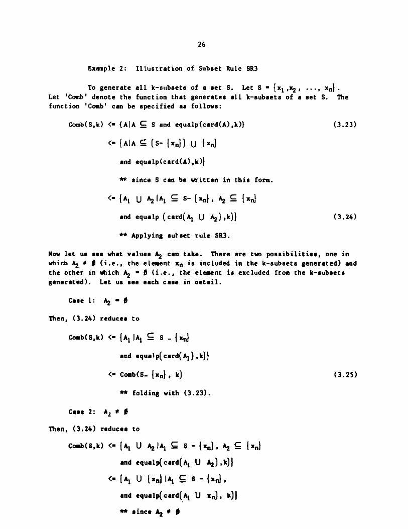
Example 2: Illustration of Subset Rule SR3

To generate all k-subsets of a set S. Let S - jx1 ,x2, - --. , xn}Let 'Comb' denote the function that generates all k-subsets of a set S. The

function 'Comb' can be specified as follows:

Comb(S,k) < (A|A C S and equalp(card(A),k)) (3.23)

<- JAIA C (S- {xnI) U jXnJ

and equalp(card(A),k)}

** since S can be written in this form.

<- {A1 U A2lIA A S- {xn}, A2 C txn

and equalp (card(A 1 U A2 ),k)I (3.24)

** Applying su-set rule SR3.

Now let us see what values A2 can take. There are two possibilities, one in

which A2 * 0 (i.e., the element xn is included in the k-subsets generated) and

the other in which A2 - 0 (i.e., the element is excluded from the k-subsets

generated). Let us see each case in detail.

Case 1: A2 - 0

Then, (3.24) reduces to

Comb(S,k) <- (A1 IAl S - {ixnI

and equalp(card(Al) ,k)}

<- Comb(S. (xn}, k) (3.25)

** folding with (3.23).

Case 2: Al * 0

Then, (3.24) reduces to

Comb(S,k) <- {A1 U A2IAl C S - ( x , A2 C (XnI

and equalp(card(A1 U A2 ),k)}

<- {Al U (xn)lA S - (xn ,

and equalp(card(A 1 U xn), k)}

**since A2 * 0

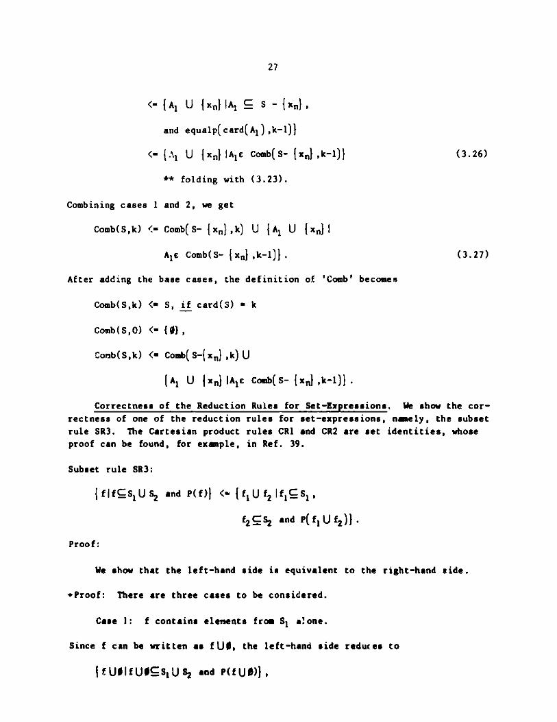
27

<- { Al U { xn} IA S - { xn} ,

and equalp(card(A 1),k-1))

<- {A1 U {xn} IAe Comb(S- {xn},k-1)} (3.26)

** folding with (3.23).

Combining cases 1 and 2, we get

Comb(S,k) <= Comb(S- {xn},k) U {Al U {xn})I

Ae Comb(S- txnI ,k-1)}. (3.27)

After adding the base cases, the definition of 'Comb' becomes

Comb(S,k) <= S, if card(S) = k

Comb(S,O) < (0),

Comb(S,k) <= Comb(S-{xn} ,k) U

{Al U {xn} IAgc Comb(S- {xn},k-1)}

Correctness of the Reduction Rules for Set-Expressions. We show the cor-

rectness of one of the reduction rules for set-expressions, namely, the subset

rule SR3. The Cartesian product rules CR1 and CR2 are set identities, whose

proof can be found, for example, in Ref. 39.

Subset rule SR3:

{ fIfcS1U S2 and P(f)I <,{ f1 U f2 If 1cS1 ,

f2 C S2 and P(f 1 U f2 )I}.

Proof:

We show that the left-hand side is equivalent to the right-hand side.

+Proof: There are three cases to be considered.

Case 1: f contains elements from S alone.

Since f can be written as fUO, the left-hand side redues to

{fU6fU s1Us2 and P(fUO)},

28

i.e.,

{fUIfcS1 , 0cS2 and P(fU0)},

since f contains elements from S1 only and 0 is a subset of all sets. This is

in the same form as the expression on the right-hand side.

Case 2: f contains elements from S2 alone.

Proof is the same as above.

Case 3: f contains elements from S1 as well as S2.

f can be written as f - fiUf2 ,

where f1 contains elements from Si alone, (i.e., fiCSi) and f2 contains ele-

ments from S2 alone (i.e., f2CS2 ).

Then, the left-hand side reduces to

{ f1 U 22I f i U f2 cS1 U S2 , and P(f 1 U f2 ) },

i.e.,

{ f1 U f2 If1CSi, f2CS 2 , and P(f1 U f 2 )}J,

since fi1CS1 , f2 9S2 by definition.

+Proof: Again there are three cases to be considered.

Case 1: fi - 0 and f2 * 0.

Then, the right-hand side reduces to

{0Uf2 I09cS1 , f2 CS2 and P(0Uf 2)},

i.e.,

{ f2 IOU f2 CS1 U S2 and P(f2)J},

i.e.,

{f2 If 2 - iUS2 and P(f2)}.

Case 2: fl * 0 and f2 n'0.

The proof is same as above.

29

Case 3: f1 * 0$and f2 * 0.

Let f denote f1 Uf2 . Since f1 CS1 and f2C;S2 , it follows that f S1 US2 .Then, the right-hand side reduces to

{ff9S1 US2 and P(f)}.

Hence the proof.0

3.2 Multiple Refinement

In our methodology, we start with the problem definition in first-order

recursion equation language and then successively transform it into a set of

algorithms, by applying the transformation rules and reduction rules for set-

expressions explained in the previous section. In the process, we carry out

multiple refinements on the algorithms for the subproblems of a given problem.

We now illustrate, by means of an example, the notion of multiple refine-

ment. A more elaborate application is presented in the next chapter. The

treatment in the example here is less formal, since our purpose is to explain

the notion briefly and clearly.

Example:

To define the predicate 'occursp,' which takes an element x and a se-

quence S as arguments and returns 'true' if x occurs in the sequence S and

'false' otherwise.

Recall that the predicate 'occursp' was used in the Section 3.1.2.1. IL

is that predicate which we shall define in this example.

Let 'first' denote the function, assumed to be primitive, that returns

the first element of a given sequence. Consider the subproblem of testing

whether a given element x occurs in the first position of each sequence of a

given set of sequences. Let 'eqfirst' denote the function that returns 'true'if the element x occurs as the first element of (at least) one of a given set

of sequences, and 'false' otherwise. Such a function can be defined as

follows-

eqfirst(x,0) <" false

eqfirst(x,.') <" true, if x " first(one(S))

<" eqfirst(x,rest(&,one(S))), otherwise.

Now consider another subproblem, namely, that of generating a set of se-quences which, when used as the second argument of 'eqfirst,' will give us the

30

answer for 'occursp.' In other words, each element of the original sequence

occurs as the first element in one of these sequences. We show two ways ofgenerating these sequences. As a result, further refinement of the problem

'occursp' in t'o directions is possible.

Refinement 1: Generation of Sequences by Rotation

Given a sequence, let 'rotate' denote a function that generates the set

of all distinct sequences obtained by rotating the sequence. The cardinality

of the set is equal to the length of the given sequence. The function

'rotate' can be defined as shown below:

rotate(S) ( rotgen(length(S),S)

rotgen(0,S) <= 0

rotgen(n,S) <{ (S) U rotgen(n-l,rest(S) 8[first(S)J).

Here, the function 'length' returns the length of a given sequence. The

auxiliary function 'rotgen' is used to actually generate the set of sequences

by rotation.

Now the functions 'rotate' and 'eqfirst' can be combined to define the

predicate 'occursp' as follows:

occursp(x,S) <* eqfirst(x,rotate(S))

eqfirst(x,O) <= false

eqfirst(x,') <= true, if x - first(one(4))

< eqfirst(xrest(S',one(S))), otherwise.

rotate(S) <= rotgen(length(S),S)

rotgen(O,S) <m 0

rotgen(n,S) <w (S)Urotgen(n-1,rest(S) 8(first(S)J).

Refinement 2: Generation of Subsequences of a Sequence

Given a sequence 8, let 'subseq' denote a function that generates the set

of all final nonempty subsequences. The cardinality of the set is equal to

the length of the given sequence. The function 'subseq' can be defined asshown below:

subseq(S) <= subseggen(length(S),S)

subseggen(0,S) < 0

subseqgen(n,S) <" (S) U subseqen(n-,rest(s)).

31

The auxiliary function 'subseqgen' is used to actually generate the desiredsubsequences.

Now the predicate 'occursp' can be defined by combining 'eqfirst' and'subseq,' as shown below:

occursp(x,S) <= eqfirst(x,subseq(S))

eqfirst(x,O) <= false

eqfirst(x,S') <= true, if x - first(one(S'))

<= eqfirst(x,rest(sone(~'))), otherwise

3ubseq(S) <= subseqgen(length(S),S)

subseqgen(O,S) <_ 0

subseqgen(n,S) <_ (S) U subseqgen(n-1,rest(S)).

32

CHAPTER 4

DERIVATION OF PERMUTATION GENERATION ALGORITHMS

In this chapter, we apply the methodology developed in the previouschapter to the problem of generating all permutations of the elements of a

given set. Working in the 'multiple refinement' style, we present two alter-native solutions to a subproblem at each refinement step, thereby yielding a

binary tree of algorithm schemata. At most steps, there are a multitude ofother solutions possible which are not considered. We choose just two repre-sentative solutions to illustrate the development. The illustrative develop-ment yields sixteen variant algorithms. The chapter concludes with a

discussion of two closely related studies, namely, Darlington's synthesis of

sorting algorithms9 and Sedgewick's compendium of permutation algorithms.3 5

4.1 Recursive Permutation Algorithms

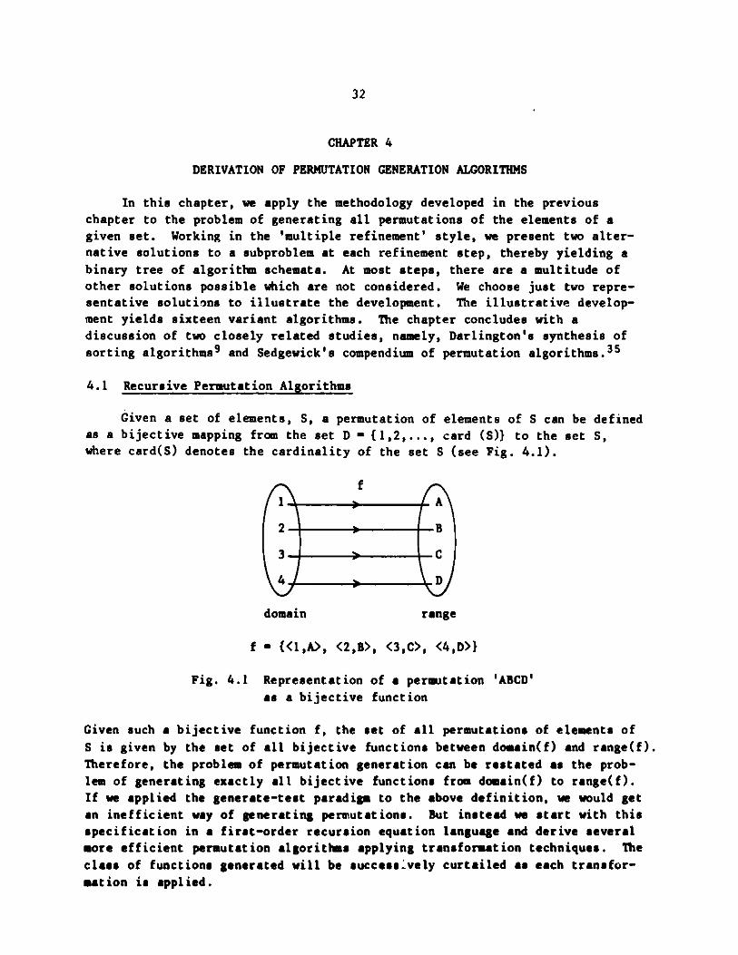
Given a set of elements, S, a permutation of elements of S can be definedas a bijective mapping from the set D = (1,2,..., card (S)} to the set S,where card(S) denotes the cardinality of the set S (see Fig. 4.1).

f

1 i A

2 aB

3 3 C

4 D

domain range

f - {<1,A>, <2,B>, <3,C>, <4,D>}

Fig. 4.1 Representation of a permutation 'ABCD'as a bijective function

Given such a bijective function f, the set of all permutations of elements of

S is given by the set of all bijective functions between domain(f) and range(f).

Therefore, the problem of permutation generation can be restated as the prob-

lem of generating exactly all biject ive functions from domain(f) to range(f).If we applied the generate-test paradigm to the above definition, we would getan inefficient way of generating permutations. But instead we start with thisspecification in a first-order recursion equation language and derive severalmore efficient permutation algorithms applying transformation techniques. The

class of functions generated will be successively curtailed as each transfor-mation is applied.

33

4.1.1 Outline of the Derivation

Given a set S of elements to be permuted, we assume a base mapping F:D +

S (or, S + D). Such a mapping induces a total order on S; i.e., for si, s2 eS,

s1 < s2, iff their images (or, preimages) d1, d2 exhibit the same relation,namely, d1 < d2 . The set of all permutations of elements of S can be obtainedfrom either the set of all bijective functions of the type D + S or the set ofall bijective functions of the type S + D. So, the set of all permutations of

elements of S can be schematically specified as follows:

Perm(F) <_ {F1I F1 domain (F) x range (F), and

Bijp (F 1 , domain (F), range (F))I where

(domain (F), range (F)} {S,D}. (4.1)

Note that the underlined words denote schema names. Instantiating (4.1) with

F = 0, we get

Perm(F) <_ {F1 F1 domain (0) x range (0) and

Bijp (F1 , domain (0), range (0))I

<_ {}. (4.2a)

Instantiating (4.1) with F = (<u,v>}, we get

Perm({<u,v>}) < {F1 IF1 C domain({<u,v>}) x range ({<u,v>}) and

Bijp (F, domain({<u,v>}), range({<u,v>} ))I

< {{<u,v>}}. (4.2b)

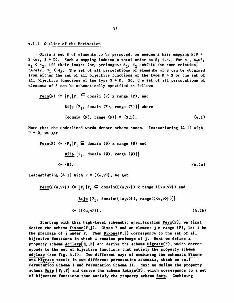
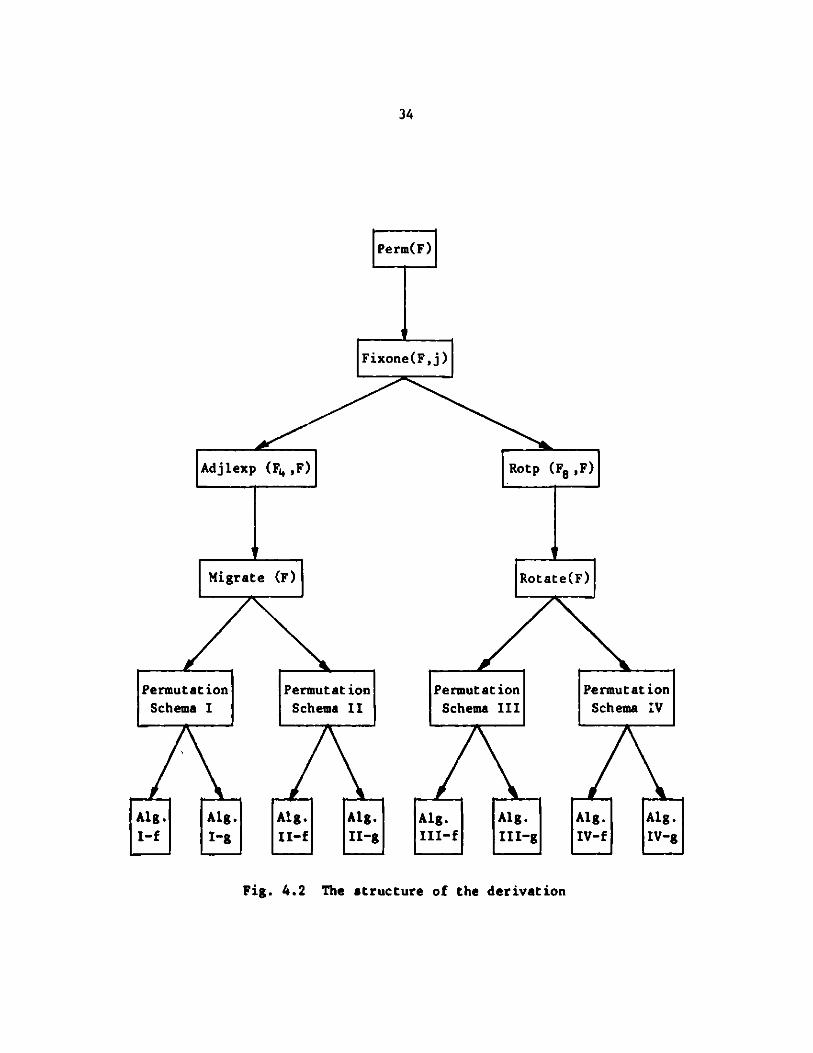
Starting with this high-level schematic specification Perm(F), we first

derive the schema Fixone(F,j). Given F and an element j e range (F), let i bethe preimage of j under F. Then Fixone(F,j) corresponds to the set of all

bijective functions in which i remains preimage of j. Next we define aproperty schema Adjlexp(F ,F) a-ad derive the schema Migrate(F), which corre-sponds to the set of bijective functions that satisfy the property schemaAdjlexp (see Fig. 4.2). Two different ways of combining the schemata Fixoneand Migrate result in two different permutation schemata, which we call

Permutation Schema I and Permutation Schema II. Next we define the property

schema Rot (F8 ,F) and derive the schema Rotate(F), which corresponds to a set

of bijective functions that satisfy the property schema Rotp. Combining

34

Perm(F)

Fixone(F,j)

Adjlexp (F4 ,F) Rotp (F8 ,F)

Migrate (F) Rotate(F)

Permutation Permutation Permutation PermutationSchema I Schema II Schema III Schema IV

Alg. Alg. Alg. Alg. Alg. Alg. Alg. Alg.

I-f I-g II-f II-g III-f III-g IV-f IV-g

Fig. 4.2 The structure of the derivation

35

Rotate and Fixone in two different ways results in two different permutation

schemata, which we call Permutation Schema III and Permutation Schema IV.

4.1.2 Derivation of Subschemata Fixone, Migrate, and Rotate

Let s - first(domain(F)),

t - F(s),

81 =succ Cs),

t1 F(s1),

r F - {<s,t>} - {<s1,t1>},

A range(F) - (t,ti),

N - domain(F) - {s}

B - tt + A.

We define below several relations between bijective functions from domain

(F) to range (F). Each such relation X(F,H) induces a set of functions

{HH = domain(F) x range(F),

Bijp (H,domain(F), range(F)), and X(F,H)}.

Three such instances appear in the three subsections below.

4.1.2.1 The Schema Fixone

Given F and an element j e range(F), let i = preimage(j) in F. Let K =domain(F) - (i}, and C = range(F) - (j}. The first rel '.on we consider is

that the preimage of j should remain fixed. Let us generate only those bijec-tive functions in which i remains the preimage of j. Let the resulting set ofobjective functions be denoted by Fixone. Since j can be arbitrarily chosenfrom range(F), we will have j as an argument to Fixone. Imposing the aboverestriction in (4.1), we can write Fixone as follows:

Fixone(F,j) <_ {F2 |F2 = (i+K) x (j+C), and

Bijp(F2 ,i+K,j+C), and

(preimage(j) in F2 - preimage(j) in F)}

36

<_ {F2 1F2 C {<i,j>) U (K x C), and

Bijp(F2 ,i+K,j+C)I

<_ { F2 U F3 IF2 C {<i, j>}, F3 C K x C,

and Bi jp( F2 U F3 , i+K, j+C)}

** using rule SR3

<_ {{<i,j>} U F3 IF3 C K x C, and

Bijp({<i, j>} U F3 ,i+K, j+C)}

** since both F2 and F3 have to

** be non-null, as otherwise

** Bijp(F2 U F3 ,i+K, j+C) will be

** false.

<_ {{<i,j>} U F3 IF3 C K x C,

Bij({<i,j>} ,i,j),

and Bijp(F3 ,K,C)} .

Breaking down the bijective filter Bijp this way is possible since

domain({ <i, j>}) and domain(F3 ) are disjoint and range({(<i, j>}) and range(F3 )

are disjoint:

<- {{<i,j>} U F3 I

F3 C domain(F-{<i, j>}) x range(F-{<i, j>}), and

Bij(F3 ,domain(F- {<i, j>} ), range(F- {<i, j>) ))I

<- {{<i, j>} U F31 F3 C Perm(F-{(<i, j>} )) (4.3)

** after folding with (4.1).

37

4.1.2.2 The Schema Migrate

The second relation we consider is the Adjlexp property shown below. Letus generate only those bijective functions that satisfy the property schema

Adjlexp:

Adjlexp(F4 ,F) <= V <u,v> c F4

v = F(first(domain(F))), or

F- 1 (v) { (u,succ(u)}. (4.4)

This property is the adjacency property if F:D + S and the lexicographicproperty if F:S + D. Let Migrate denote the class of bijective functions thatsatisfy the above property schema. Imposing this property schema in (4.1), we

get

Migrate(F) <_ {F4jF4 domain(F) x range(F),

Bijj_(F 4 ,domain(F), range(F)),

and Adjlexp(F4 ,F)}

< ngeF({<domain <s,t>,<s1,t1>,r})

x range({<s, t>,<s1,t 1>,r}1 ,

Bijp(Fg ,domain({ <s, t>,<si , t1i> ,r} ) ,

range({<s,t>,<s 1 ,t1 >,r}))

and Adjlexp(F4 ,F)} (4.5)

** using s,t,s1 ,t1 ,r defined in

** the beginning of Sec. 4.1.2.

In order to simplify (4.5), let us rearrange the terms contributed by

domain(j<s,t> , <s1,t1>, r}) x range((<s,t>, <s1,t1>, r}) as shown below:

domain({<s,t> , <siti> , r})

x range({<s,t> , <s1 ,t> ,r}) s (s+N) x (t+t1 +A)

- {<s,t>} U {<s,ti>} U

(s) x A U (N x (t)) U

(N x (ti}) U (N x A) (4.6)

** using rule CR2.

38

Let us replicate N x A in (4.6) and rearrange the union operations as shown

below:

S{<s,t>} U (N x {t1}) U (N x A) U {<s,t1>} U

({s} x A) U (N x {t}) U (N x A) (4.6a)

Let

S1 = {<s,t>} U (N x {t1 }) U (N x A),

S2- {<s,ti>} U ({s) x A) U (N x {t}) U (N x A).

Then (4.6) can be written as S1 U S2.

Now using (4.6) and (4.6a), we can rewrite (4.5) as

<- {F4 IF4 C S1 U S2 >

Bij(F4 ,s+N,t+B) ,

and Ad jlexp(F4 ,F) },

and further using rule SR3,

<_ {F5 U F61F5 C {<s,t>} U N x (t1 + A)

F6 C {<s,t1 >} U (s} x A U N x (t+A),

Bijp(F5 U F6 ,s+N,t+t 1 +A)

and Adjlexp(F 5 U F6 ,F)} . (4.7)

Let us now see what values F5 and F6 can take:

Case 1: F5 # 0 and F6 = 0

Case 2: F5 0 and F6 * 0

Case 3: F5 # 0 and F6 0

For case 1, (4.7) reduces to

39

<_ (F5 |F5 C {<s,t>} U N x (t1 +A),

Bj(F 5 ,s+N,t+t1+A),

and Adjlexp(F5 ,F)}

<_ {{<s,t> , <s 1 ,t 1> ,r}}

** since in all other cases the

** property schema Adjlexp will

** be violated.

< {F).

For case 2, (4.7) reduces to

<_ {F 6 IF6 C {<s,t 1>} U {s} x A U N x (t+A),

B~ij(F6 ,s+N,t 1 +t+A),

and Adjlexp(F6 ,F)I

<= {{<s,t 1>} U F7IF7 C N x (t+A),

Bijp({<s,t1>} U F7,s+N,t1+t+A),

and Adjlexp({<s,t 1>} U F7 ,F)}

** by rule SR3.

Note that the set {s} x A is not considered in computing F7. This is because

its inclusion will violate the function property, as a is already mapping onto

tie We get

<_ {{<s,t1>} U F7IF7 C N x (t+A),

Bij(F7 ,N,t+A), and

Adjlexp(F7 ,F)

** after breaking down the Bijj

** function.

The above is valid because domain and range of {<s,t 1>} and F7 are disjoint.Breaking Adjlexp is also consistent with the definition of Adjlexp given in

40

(4.4). Now, as N - domain({<s1 ,t> ,r)), and (t+A)=range({<si ,t>, r}) , we get

<_ {{<sti>} U F7 |F7 C domain((<s 1 ,t>,r}) x range(j<s1 ,t>,r}),

Bi(F7 ,N,t+A) and

Adjlexp(F 7 ,{<s,t>, r})} . (4.8)

In order to introduce a fold, we have to rewrite the second argument of

Adjlexp in (4.8) as Adjlexp(F 7 ,{ <s1 ,t>,r})). This rewriting is consistent withthe definition of Adjlexp given in (4.4) because si = first(domain({<s1 ,t>,r}))

and t is image(s1). After a fold is introduced, (4.8) becomes

<_ {{<s,ti>} U F7 |F7 e Migrate({<s1 ,t>,r})}.

Case 3: Both F5 and F6 are not null:

F5 C S1, and F6 C 2

where

S ={<s,t>} U (N x {ti}) U (N x A)

S2 = {<s,t 1 >} U ((s} x A) U (N x {t}) U (N x A).

Note that N x A occurs both in S and S2.

Suppose we choose {<s,t>} from S for F5 . Then we are bound to choose

{ <s1 ,tl>} from S for F5 , since there is no legal t<u,ti>} in S2 which, whencombined with {<s,t>}, will not violate Bijp and Adjlexp properties. Having

chosen {<s,t>, <s5 ,t1>}, we are left with only r from N x A, as the rest of itthat is, (N x A - r) will violate the Adjlexp property. This subset can be

chosen from N x A of either Si or S2. We need not consider the choice from S2since this is already absorbed in case 1. Similarly, if we choose {<si ,t1>}from S , then we are bound to choose {<s,t>} also from Si for F5 , and the samecase as above results.

The only other possibility is to choose some subset of N x A from Si for

F5 and some subset of S2 and consider their union. Since N x A occurs in S2also, it is enough if we consider the subset of S2 alone. This is absorbed in

case 2, which we considered earlier.

Thus, we need not consider the case F5 U F6 where both F5 and F6 are notnull, since the functions they compute occur either in case 1 or case 2.

Hence, Migrate(F) can be rewritten retaining only case 1 and case 2:

41

Mijrate(F) <_ {F} U {{<s,ti>} U F7jF7 E Migrate( {<s1,t>,r})}.

After adding the base case, we obtain the following definition of Migrate:

Migrate({<u,v>}) <_ {{<u,v>}}

Migrate(F) <_ {F} U {{<s,t1>} U F7 |F7 c Migrate({<slt>,r})}.

4.1.2.3 The Schema Rotate

The third relation we consider is the property schema Rotp shown below:

Rotp(F8 ,F) <= 3m, -1 < m < card(domain(F)), such that V <u,v> c F8,

V-= F(succ'm (u)), (4.9)

where succ' is the circular successor function

succ'(u) = succ(u), for all u,u < last(domain(F))

and

succ'(last(domain(F))) = first(domain(F)).

The property Rotp induces a set of functions Rotate(F), for a givenfunction F:

Rotate(F) <_ {F9 |F9 = domain(F) x range(F),

Bijj(F9,domain(F),range(F)), and

Rtp(F9,F)}

<_ {{<u,v>Iu E domain(F) and

v = F(succ'm (u))I,

for -1 < m < card(domain(F))}

** from the definition of

** property schema Rotp.

4.1.3 Derivation of Different Permutation Schemata

We derive different permutation schemata by suitably combining thedifferent subschemata derived in the previous section. Given F, let

v - F(first(domain(F))). (4.10)

42

4.1.3.1 Derivation of Permutation Schemata I and II

We combine the subschemata Fixone and Migrate and derive Permutation

Schemata I and II. We use the following construction in showing that the

combination yields permutation schemata.

Construction:

Given any function Fi and a (total) ordering of its domain, let Mi be a

function, defined for ill d e domain(Fi) as follows:

Mi(d) <_ {<a,b>la a domain(F i),

bik, if a -=d,

b=Fi(succ(a)), if a < d,

b-Fi(a), if a > d.1

where

k-Fi(first(domain(Fi))). (4.11)

We invoke this construction with two functions, namely, F and F1 1 , in the

subsequent sections. Hence, the symbols Fi and Mi above are used in a generic

sense and will be instantiated by a pair of matching M and F symbols, e.g.,

(M,F) and (M11,F11), when needed.

Informally, Mi defines a set of functions that satisfy Adjlexp property,

i.e., V d e domain(F), Adjlexp(Mi(d),Fi) is true. From (4.11) it follows that

Preimage (Fi(first(domain(Fi))) in Mi(d) - d. (4.12)

Permutation Schema I. Let us apply Fixone to each of the bijective

functions resulting from applying Migrate to F. For the moment, let us denote

the resulting set of bijective functions by Perm'(F). We shall show that it

is the same as Perm(F). Thus, we have

Perm'(F) <- U Fixone(F1 0 ,v)F10e Migrate(F), (4.13)

where

v1 is as defined in (4.10).

Proof: by construction.

43

From (4.11) and (4.12), it follows that the functions M(d) for all d edomain(F) satisfy the Bijp and Adjlexp properties (see the definition of

Adjlexp given in (4.4)). From (4.12), it can be inferred that the functions

M(d) are all distinct. There are card(domain(F)) functions 'fined by M(d).

Since Migrate(F) produces a set of bijective functions with Adjlexp property

satisfied, it should contain at least card(domain(F)) distinct functions

defined by M(d).

From the definition of Fixone and (4.11), it follows that

Vd1 , d2 e domain(F),

Fixone(M(d 1 ), v1) fl Fixone(M(d 2) ,v1) = 0. (4.14)

For each d e domain (F), Fixone (M(d),v ) generates one function for each

bijective function from (domain(F)- {d}) to ?range(F) - {v}j). We know thatthere are (n-1)! functions from (domain(F) - {d}) to (range (F) - {v1}) .Equation (4.14) and the fact that Migrate (F) has at least card(do.nain(F))

(i.e., n) distinct bijective functions defined by M(d), together imply that

Perm', as defined in (4.13), generates at least n.(n-1)! =n! unique bijective

functions from domain(F) to range (F). In other words, it generates all

permutations, and hence Perm'(F) is the same as Perm(F). 0

Thus, the Permutation Schema I is

Perm (0) < {0}

Perm({<u,v>}) <= {{<u,v>}}

Perm(F) <= U Fixone(F 1 0 v1

F10e Migrate(F)

Fixone(F1 0 ,v1 ) <_ {{<i,v1>} U F3 1I F3 Perm (F10-{ <iv>}) }

where i = preimage(v 1 ) in F10

Migrate({<u,v>}) ( <{{<u,v>}}

Migrate(F) <_ {F} U {{<s,ti>} U F71 F7 a Migrate((<s1 ,t>,rI))

44

Permutation Schema II. Let us apply Migrate to each of the bijective

functions resulting from applying Fixone to F. For the moment, let us denotethe resulting set of bijective functions by Perm''(F). We shall show that it

is the same as Perm(F). Thus, we have

Perm''(F) <- U Migrate(Fl )F1 Fixone(F,v1 ), (4.15)

where v1 is as defined in (4.10).

Proof: by construction.

From (4.11) and (4.12), it follows that, for any F11 e Fixone (F,v 1 ), thefunctions M 1(d) for all d e domain(F1 1) satisfy the Bijp and Adjlexp proper-

ties (see the definition of Adjlexp given in (4.4)). From (4.12), it cau beinferred that the functions M1 1id) are all distinct. There are card(domain

(F1 1 )). functions defined by M1 1 (d). Since Migrate(F11) produces a set ofbijective functions with Adjlexp property satisfied, it should contain at

least card(domain(F1 1)) distinct functions defined by M11 (d). Note that

card(domain(F11 )) is the same as card(domain(F)), since Fixone generates a set

of bijective functions from domain(F) to range(F).

Lemma 1:

For any F1 2 ,F 1 2 ' e Fixone(F,v1 ) , F1 2 * F1 2 ', M12(d1) * M12 '(d2)V dd 2 a domain(F1 2 ) .

Proof: Only the following two cases need be considered.

Case 1: d1 * d2

By definition of M1 2 , dl is the preimage of v1 in M1 2 (dl) and d2 is thepreimage of vl in M1 2 '(d 2); hence, the two bijective functions are not equal.

Case 2: d1 - d2, ("d, say)

From the definition of Fixone (F,v1), it follows that there exists w such

that

w c range(F), w * v1 , and

preimage(w) in F12 * preimage(w) in F12'. (4.16)

Let u and u' be the preimages of w in M12(d) and M1 2'(d), respectively. There

are essentially the following four cases to be considered:

Case a: u < d and u' > d

45

This implies that u * u' and, hence,

M12(d) * M12 '(d)

Case b: u > d and u' < d

This again implies that u * u' and, hence,

M 1 2 (d) * M1 2 '(d)

Case c: u < d and u' < d

From (4.11) and (4.12), it follows that

preimage(w) in F12 s succ(u), preimage(w) in F12 ' - succ(u').

From (4.16), it follows that succ(u) * succ(u'), which in turn impliesthat u * u'. Hence,

M1 2 (d) # M12'(d).

Case d: u > d and u' > d

From (4.11) and (4.12), it follows that

preimage(w) in F1 2 - u, preimage(w) in F12 ' - u'.

Fsom (4.16), it follows that u * u' and, hence,

M 1 2 (d) * M1 2 '(d). Q

Fixone(F,v1 ) generates one function for each bijective function from

(domain(F) - (i)) to (range(F) - lvii). We know that there are (n-1)! func-tions from (domain(F)- i}) to (range(F) - {v1}). Lemma 1 and the fact thatMigrate (F11) has at least card(domain(Fl 1 )), (i.e., n), distinct bijectivefunctions defined by M1 1 (d) together imply that Perm'', as defined in (4.15),produces at least n.(n-1)!"n! unique bijective functions from domain(F) to

range(F). In other words, it generates all permutations, and hence Perm''(F)

is the same as Perm(F). 0

Thus, the Permutation Schema II is

Perm(0) < (0)

Perm({<u,v>}) < {{<u,v>}}

Perm(F) <- U Migrate(F 1 )F11c Fixone (F,v1)

46

Fixone (F,v 1 ) < {{<i,v1 >} U F3 | F3 c Perm (F- (<i,vi >)f

where i - preimage (v 1 ) in F

Migrate({<u,v>}) < {{<u,v>}}

Migrate(F) <_ {F) U {{<s,t1 >} U F7 1

F7 Migrate({ (s1 , t>,r})).

4.1.3.2 Derivation of Permutation Schemata III and 1V

We combine the subschemata Fixone and Rotate and derive Permutation

Schemata III and IV. We use the following construction in showing that the

combination yields permutation schemata.

Construction:

Given Fi, let R be a function defined as follows:

R( Fi) <_ { <a, b>|Ia c domain( Fi) ,

b - Fi(succ'(a))}.

Let R*(Fi) denote the set

{Fi,R(Fi),R(R(Fi)), ... , R(m-1) (Fi)},

where

m - card(domain(F)).

Since RP(Fi) * Rq(Fi) for p # q, -1 < p , q < m, it follows that

card(R*(Fi)) = m = card(domain(Fi)). (4.17)

Further, the functions in R*(Fi) satisfy Bijp and Rot properties and are

all distinct. There are card(domain(Fi)) functions in R* Fi) . SinceRotate(Fi) produces the set of all bijective functions with Rotp property

satisfied, it should contain at least the card(domain(Fi)) distinct functionswhich are in R*(Fi) .

Permutation Schema III. Let us apply Fixone to each of the bijective

functions resulting from applying Rotate to F. For the moment, let us denote

47

the resulting set of bijective functions by Perm'''(F). We shall show that itis the same as Perm(F). Thus, we have

Perm'''(F) < U Fixone( F1 2,v1)

F12e Rotate(F), (4.18)

where v1 is as defined in (4.10).

Proof: by construction

Rotate(F) contains at least card(domain(F)) distinct functions which are

in R*(F).

From the definition of Fixone and the fact that v1 has distinct preimagesin each of the functions in R*(F), it follows that, for any F13 ,F14 c R*(F),

Fixone(F1 3 ,v1) fl Fixone(F1 4 ,vI) - 0. (4.19)

Given a function F13 e R*(F), Fixone(F1 3 3v1) generates one function for

each bijective function from (domain(F)- {i}) to (range(F) - {vl}), where i isthe preimage of v1 in F1 3. We know that there are (n-1)! such functions.Equation (4.19) and the fact that Rotate(F) has at least card(domain(F))

(i.e., n) distinct bijective functions as defined by R*(F) together imply thatPerm''', as defined in (4.18), generates at least n.(n-1)! - n! unique

bijective functions from domain(F) to range(F). In other words, it generates

all permutations, and hence Perm'''(F) is the same as Perm(F). Thus,

Permutation Schema III is

Perm($) < {}

Perm({<u,v>}) ( {{<u,v>}}

Perm(F) <- U Fixone(F 1 2 ,v 1 )F12e Rotate(F)

Rotate(F) <_ {{ <u,v>Iuc domain(F) and v = F(succ'm(u))},

for m,-1 < m < card(domain(F))

Fixone(F 1 2 ,v 1) (_{{(iv1>} U F3 1 F3 Perm(F12- {<iv 1>})}

where iipreimage(v 1 ) in F1 2 .0

48

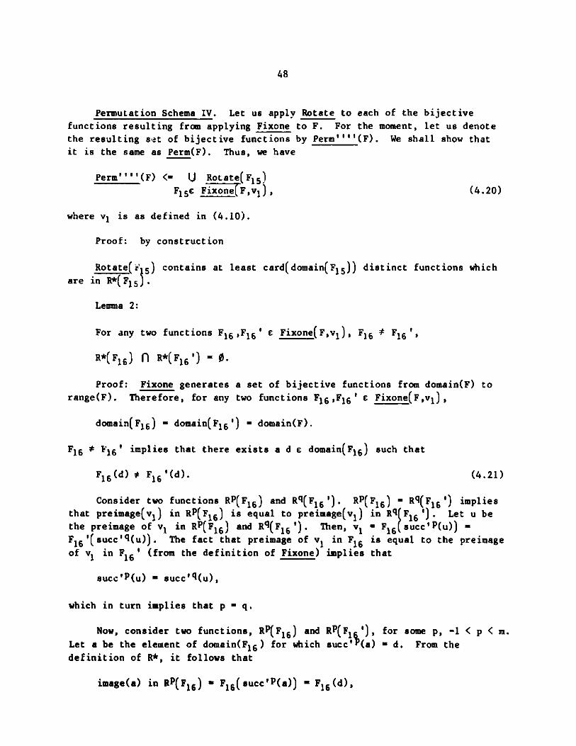
Permutation Schema IV. Let us apply Rotate to each of the bijectivefunctions resulting from applying Fixone to F. For the moment, let us denotethe resulting set of bijective functions by Perm''''(F). We shall show thatit is the same as Perm(F). Thus, we have

Perm''''(F) <_ U Rotate(F1 5 )F1 5c Fixone(F,vj) , (4.20)

where v1 is as defined in (4.10).

Proof: by construction

Rotate( r' 5 ) contains at least card(domain(F1 5)) distinct functions whichare in R*(F1 5 )-

Lemma 2:

For any two functions F1 6 ,F 1 6 ' e Fixone(F,v1 ), F1 6 *F16 1 ,

R*(F1 6 ) fl R*(F1 6 ' - 0'

Proof: Fixone generates a set of bijective functions from domain(F) to

range(F). Therefore, for any two functions F1 6 ,F 1 6 ' c Fixone(F,v1),

domain(F 1 6 ) - domain(F1 6 ') - domain(F).

F1 6 * F1 6' implies that there exists a d c domain(F16) such that

F1 6 (d) * F1 6 '(d). (4.21)

Consider two functions RP(F1 6 ) and R(F1 6 ') . RP(F1 6 ) = R(F1 6 ') impliesthat preimage(v1 ) in RP(F1 6 ) is equal to preimage(v 1 ) in R (F16 ') . Let u bethe preimage of v1 in RP(F1 6 ) and R(F 1 6 ') . Then, v1 - F1 6 (succ' P(u)) -F1 6 '(succ'q(u)) . The fact that preimage of v1 in F16 is equal to the preimageof v1 in F1 6' (from the definition of Fixone) implies that

succ'p(u) - succ'q(u),

which in turn implies that p - q.

Now, consider two functions, RP(F1 6 ) and RP(F16 '), for some p, -1 < p < m.Let a be the element of domain(F1 6 ) for which succ' P(a) - d. From thedefinition of R*, it follows that

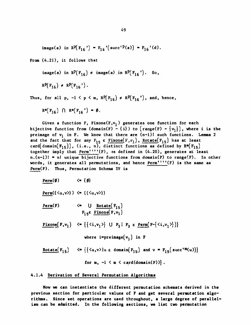
image(a) in RP(F16) a F16(succ'P(a)) - F16(d),

49

image a) in RP(F1 6 ') = F1 6 '(succ'P(a)) = F1 6 '(d).

From (4.21), it follows that

image(a) in RP(F1 6 ) * image(a) Jin RP(F1 6 '). So,

RP(F1 6 ) * RP(F1 6 ') .

Thus, for all p, -1 < p < m, RP(F1 6 ) * RP(F1 6 '), and, hence,

R*(F1 6 ) fl R*(F 1 6 ') 0.

Given a function F, Fixone(F,v1 ) generates one function for each

bijective function from (domain(F) - (i}) to (range(F) - {v1}), where i is the

preimage of v1 in F. We know that there are (n-1)! such functions. Lemma 2

and the fact that for any F1 5 a Fixone(F,v 1 ), Rotate(F1 5 ) has at leastcard(domain(F 1 5 )), (i.e., n), distinct functions as defined by R*(F1 5 )together imply that Perm''''(F), as defined in (4.20), generates at least

n.(n-1)! = n! unique bijective functions from domain(F) to range(F). In other

words, it generates all permutations, and hence Perm''''(F) is the same as

Perm(F). Thus, Permutation Schema IV is

Perm(0) < {0)

Perm({(<u,v>}) < ({{<u,v>})

Perm(F) <- U Rotate(F1 5)

F1 5 e Fixone(F,v 1 )

Fixone(F,v 1 ) <_ {({ i,v1 >} U F31 F3 a Perm(F-{<i,vi >})

where i=preimage(v1) in F

Rotate(F1 5 ) <_ {{<u,v>Iu e domain(F 1 5 ) and v = F1 5(succ'm(u))j

for m, -1 < m < card(domain(F)).

4.1.4 Derivation of Several Permutation Algorithms

Now we can instantiate the different permutation schemata derived in the

previous section for particular values of F and get several permutation algo-

rithms. Since set operations are used throughout, a large degree of parallel-

ism can be admitted. In the following sections, we list two permutation

50

algorithms obtained by instantiating Permutation Schema I and II, respec-

tively, and explain the order in which the permutations are generated. The

remaining algorithms obtained by instantiating Permutation Schemata I, II,

III, and IV are listed in Appendix A. These algorithms can be implemented

sequentially by generating the sets as sequences. In order to compare thesesequential algorithms, we list in Appendix B the permutation sequences gener-

ated by these algorithms for f-{<1,A>, <2,B>, <3,C>, <4,D>}.

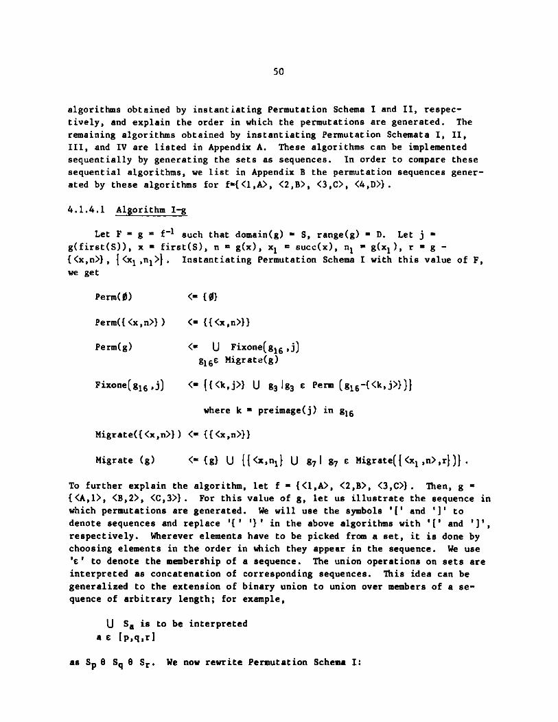
4.1.4.1 Algorithm I-g

Let F = g = f-1 such that domain(g) - S, range(g) = D. Let j -g(first(S)), x - first(S), n - g(x), x1 = succ(x), n1 = g(x1), r = g -{<x,n>}, {<x1 ,n1>}. Instantiating Permutation Schema I with this value of F,we get

Perm($) <_ {0}

Perm({<x,n>}) <_ {{<x,n>}}

Perm(g) <- U Fixone(g16,j)

g16e Migrate(g)

Fixone(g 1 6 ,j) < {{<k,j>} U g3 1g3 Perm (g16 -(<k,j>))}

where k = preimage(j) in g1 6

Migrate({<x,n>}) < {{<x,n>}}

Migrate (g) <_ {g} U I<x,n} U 97 1 g7 e Migrate({<x 1 ,n>,r})}

To further explain the algorithm, let f = {<l,A>, <2,B>, <3,C>}. Then, g ={<A,1>, <B,2>, <C,3>}. For this value of g, let us illustrate the sequence inwhich permutations are generated. We will use the symbols '[' and ']' to

denote sequences and replace '{' '}' in the above algorithms with '[' and 'J',respectively. Wherever elements have to be picked from a set, it is done by

choosing elements in the order in which they appear in the sequence. We use'e' to denote the membership of a sequence. The union operations on sets areinterpreted as concatenation of corresponding sequences. This idea can be

generalized to the extension of binary union to union over members of a se-

quence of arbitrary length; for example,

U Sa is to be interpreteda [p,q,r]

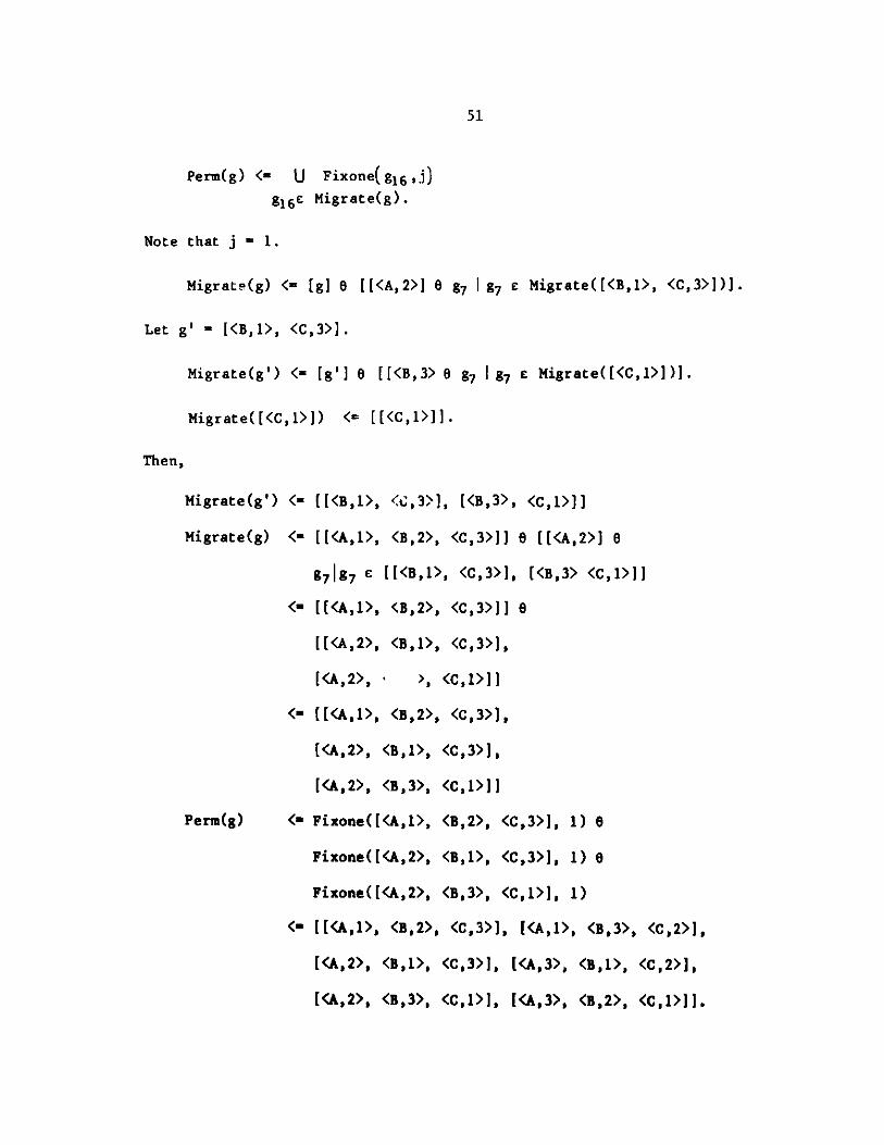
as Sp 0 Sq 0 Sr. We now rewrite Permutation Schema I:

51

Perm(g) <- U Fixone(g 1 6 >-)

g1 6e Migrate(g).

Note that j - 1.

Migrate(g) < [g] [[<A,2>] 8 g7 I g7 e Migrate([<B,1>, <C,3>J)].

Let g' - [<B,1>, <C,3>].

Migrate(g') <_ [g'] 0 [[<B,3> 0 g7 1 g7 e Migrate([<C,1>])].

Migrate([<C,1>]) << [[<C,1>]].

Then,

Migrate(g')

Migrate(g)

Perm(g)

< [([<B,1>, <C,3>], [<B,3>, <ci>]]

<_ [[<A,1>, <B,2>, <C,3>J e [[<A,2>] e

971g7 c [[<B,1>, <C,3>], [<B,3> <C,1>]]

<_ [[<A,1>, <B,2>, <C,3>] 0

[[<A,2>, <B,1>, <C,3>],

[<A,2>, ' >, <C,1>JJ

<_ [[<A,1>, <B,2>, <C,3>J,

[<A,2>, <B,1>, <C,3>J,

[<A,2>, <B,3>, <C,1>]J

<= Fixone([<A,1>, <B,2>, <C,3>], 1) 0

Fixone([<A,2>, <B,1>, <C,3>J, 1) 0

Fixone([<A,2>, <B,3>, <C,1>], 1)

<_ [[<A,1>, <B,2>, <C,3>J, [<A,1>, <B,3>, <C,2>J,

[<A,2>, <B,1>, <C,3>1, [<A,3>, <B,1>, <C,2>1,

[<A,2>, <B,3>, <C,1>j, [<A,3>, <B,2>, <C,1>]J.

52

4.4.2 Algorithm II-f

Let F = f such that domain(f) = D, range(f) = S. Instantiating

Permutation Schema II with this value of F, we get

Perm(0) <_ {}

Perm({ <n , x>}) <_{ (<n , x>}}

Perm(F) < U Migrate (f1 7 )

f1 7e Fixone(f,j)

where j = f(first(D))

Fixone(f,j) <_ {{<i,j>} U f3 1 f3 c Perm(f-{(<i,j>})}

where i = preimage(j) in f.

Migrate({<n,x>}) < {{<n,x>}}

Migrate(f17) <_ {f 1 7} U {{<n,x1 >} U f 7 I

f7 c Migrate({<n1 ,x> ,r})} ,

where

n - first(domain(f1 7 )), n1 = succ(n), x =f17(n,

x1=- f17(n1), r - f1 7 -{<n,x>} - {<n1,x1>}.

Let f - {<l,A>, <2,B>, <3,C>}. Then,

Perm(f) <= U Migrate(f17 )

f1 7c Fixone(f,j).

Note that j - A.

Fixone(f,A) <_ [[<1,A>) a f3 Ilf 3 Perm([<2,B>, <3,C>1)]).

53

Let f' - [<2,B>, <3,C>].

Perm(f') <= U Migrate(f1 7')

f17'e Fixone (f',B)

Fixone(f',B) <_ [[<2,B>] a f3 1 f3' e Perm([<3,C>])]

<_ [[<2, - >, <3,C>1]

Perm(f') <= Migrate([<2,B>, <3,C>])

<_ [[<2,B>, <3,C>], [<2,C>, <3,B>]]

Fixone(f,A) <_ [[<1,A>, <2,B>, <3,C>],

[<1,A>, <2,C>, <3,B>]]

Perm(f) <= Migrate([<l,A>, <2,B>, <3,C>]) e

Migrate([<l,A>, <2,C>, <3,B>])

<_ [[<l,A>, <2,B>, <3,C>],

[<1,B>, <2,A>, <3,C>],

[<l,B>, <2,C>, <3,A>],

[<1,A>, <2,C>, <3,B>],

[<1,C>, <2,A>, <3,B>J,

[<1,c>, <2,B>, <3,A>]].

4.2 Relation to the Work of Darlington and of Sedgewick

Our work is closely related to Darlington's recent work on synthesizing a

set of sorting algorithms.9 We differ from his approach in that we start with

an abstract schema based on the problem definition and derive a set of algo-

rithm schemata. Under different interpretations, these schemata yield differ-

ent algorithms for the same problem.

Darlington has used permutation generation as an intermediate problem

towards creating sorting algorithms. The connection between the two becomes

apparent only when the algorithms are developed. On the other hand, our

development proceeds in small steps from the definition of the problem.

54

While we cannot yet claim that most of the development process can be mecha-nized, the development follows the well-known paradigms of programming.

We apply the notion of 'multiple refinement' on the algorithms for thesubproblems of the given problem. This results in stepwise freezing of thealgorithms developed, whereas in Darlington's approach the algorithms for thepermutation subproblem are already completely 'frozen' algorithms. At each ofour steps, an abstract parent schema yields two more frozen schemata. Thusthe resulting algorithms can be seen to fit into a binary hypercube, which isshown as a Karnaugh map in Fig. 4.3.

\AB 00 01 11 10

A:B:C:D:"

rotate/migrateorder of applicationforward/reversefirst = smallest/largest

Fig. 4.3 Hypercubes of permutation algorithms

We chose two distinct methods ofand rotate. For each fresh techniqueget eight new algorithms by following

integrating the saved element: migratefor this purpose, one can immediatelythe other steps of our developments.

Sedgewick 3 5 has given a thorough survey of existing algorithms for per-mutation generation. In his survey, he relates many algorithms to a singlebasic recursive scheme which is different from any of our basic schemes.Sedgewick's recursive scheme is as follows:

Given in the array P the original permutation,

repeat n times:

begin

lint (n-1)! permutations of P[11 ... P[n-11

with P[n] retaining its position;

exchange P[nJ with the appropriate earlier element;

end.

CD

00

01

11

10

IV-f III-f II-f I-fIP1 IP1 IP1 IP1

IV-f III-f II-f I-fIP2 IP2 IP2 IP2

IV-g III-g II-g I-gIP1 IP1 IP1 IP1

IV-g III-g II-g I-gIP2 IP2 IP2 IP2

x1%

55

The 'appropriate' element with which to exchange P[n] has to be determined so

that all n! distinct permutations get listed. The choice depends on the lastshorter permutations listed. This basic scheme guarantees that each algorithmproduced requires a single exchange at each step while moving from one permu-

tation to the next. Those algorithms that do not satisfy this property (e.g.,lexicographic) have to be treated separately.

None of our algorithms has that property. It would be interesting tostudy how they can be modified to achieve it. The following algorithms appearclosest to each other:

Ours Sedgewick's

II-g-IP1 Algorithm 3

III-g (IP1 and IP2) Algorithm 5

IV-f-IP2 Algorithm 6

56

CHAPTER 5

RELATED PROBLEMS

In the last chapter, we applied our methodology to the derivation of a setof algorithms for the problem of generating all permutations of the elements of

a given set. A related class of problems requires us to generate only thosepermutations that satisfy a certain property. In this chapter, we consider

one such problem, namely, the problem of generating all permutations that areproducible using a stack. We shall call such permutations 'stack permuta-

tions.' A brute force method of generating all stack permutations is to gener-ate all the permutations of the elements of a given set and then reject thosethat do not satisfy the stack permutation property. We develop a conditionwhich guarantees that an extension of a given stack permutation through

'Migrate' is also a stack permutation. This condition is then used for step-

wise pruning of non-stack permutations so that the number of permutations

tried is significantly less than in the brute force method. The algorithmproduced is an adaptation of the algorithm II-f of the previous chapter.

Next we discuss an interesting relationship between stack permutations

and binary trees.

5.1 Stack Permutations and Tree Codes

Definition 5.1: Any permutation of 1,2,..., n that can be produced from

the sequence 1,2, ...,n using a stack to alter the sequence of elements is

said to be a stack permutation. A generalized stack permutation (hereafterdenoted as g-stack permutation) is a sequence obtained from a stack permuta-

tion by incrementing all the elements in the stack permutation by the sameconstant. For example, given the input sequence 1234, the output sequence

2431 is a stack permutation. The' sequence of elements 3542 is a generalizedstack permutation, obtained from 2431 by incrementing all the elements by 1.

The operations associated with the stack are 'push,' 'pop' and 'pass.''Push' pushes the next element in the input sequence onto the stack, 'pop'pops out the top element of the stack onto the output, and p1rs' passes thenext element in the input sequence onto the output.

Definition 5.2: A stack program is a sequence of stack operations thatoperates on the given input sequence and produces a stack permutation. Forinstance, the stack permutation 2431 above is obtained by the stack program

push, pass, push, pass, pop, pop.

In any stack PLogram, the number of 'push' operations is equal to the numberof 'pop' operations. Further, at any point, the number of 'pop' operations

cannot exceed the number of 'push' operations.

The sequence of elements resulting from feeding a sequence of ele-

marts 1,2, ... , n Lo a stack program is a st ck permutation. Alternatively,

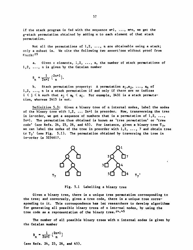
57

if the stack program is fed with the sequence m+l, ..., m+n, we get the

g-stack permutation obtained by adding m to each element of that stackpermutation.

Not all the permutations of 1,2, ..., n are obtainable using a stack;

only a subset is. We cite the following two assertions without proof from

Knuth: 25

a. Given n elements, 1,2, ... , n, the number of stack permutations of1,2, ..., n is given by the Catalan number

1 (2n+1n 2n+1 n

b. Stack permutation property: A permutation a1,a2, .'', an of1,2, ... , n is a stack permutation if and only if there are no indicesi < j < k such that aj < ak < ai. For example, 2431 is a stack permuta-tion, whereas 2413 is not.

Definition 5.3: Given a binary tree of n internal nodes, label the nodes

of the binary tree with 1,2, ... 2n+1 in preorder. Now, transversing the treein in-order, we get a sequence of numbers that is a permutation of 1,2, ... ,2n+1. The permutation thus obtained is known as 'tree permutation' or 'tree

code' (see Refs. 24, 25, 26, and 45). For instance, given a binary tree T7,we can label the nodes of the tree in preorder with 1,2, ..., 7 and obtain tree

tr T7' (see Fig. 5.1). The permutation obtained by traversing the tree in

in-order is 3254617.

1

2 7

3 4

T7 5 6

Fig. 5.1 Labelling a binary tree

Given a binary tree, there is a unique tree permutation corresponding to

the tree; and conversely, given a tree code, there is a unique tree corre-

sponding to it. This correspondence has led researchers to develop algorithmsfor generating all possible binary trees of n internal nodes, by using the

tree code as a representation of the binary tree.24,4 5

The number of all possible binary trees with n internal nodes is given by

the Catalan number

B - 1 (2n+1)n 2n+1 n

(see Rers. 24, 25, 26, and 45).

58

All possible binary trees with three internal nodes, along with tree

codes representing them, are shown in Fig. 5.2.

5.2 An Algorithm for Generating Stack Permutations

Permutation Algorithm II-f derived in the previous chapter generates the

set of all permutations by first applying Fixone to F, and then applying

Migrate to each of the functions generated by Fixone. By an adaptation ofthis algorithm, we get an algorithm that generates g-stack permutations in a

similar manner. Let 'spmigrate,' 'spfixone' and 'spperm' denote functions

analogous to the functions 'Migrate,' 'Fixone' and 'Perm' used in the permuta-

tion algorithms.

Given a g-stack permutation a1,a2, ... , an and an integer m such that

m < ai for all i, i = 1, ... , n, m a1 .... an is a g-stack permutation.

We can generate the remaining extensions of al, ... , an, which are g-stack

permutations, by allowing m to migrate to the right one position at a time.The 'Migrate' function of Permutation Algorithm II-f generates a set of permu-

tations by allowing the first element to migrate to the right. But in the

present case of generating g-stack permutations, not all the permutationsresulting from 'Migrate' will satisfy the stack permutation property. Forinstance, given the g-stack permutation 432 and m - 1, the permutations pro-

duced by 'Migrate' are 4132, 4312, 4321, of which only 4321 is a g-stack per-mutation. Therefore, we have to find a condition under which a permutation

obtained by 'Migrate' applied to a g-stack permutation is a g-stack

permutation.

We first develop the condition that should be satisfied by a permutation

obtained by 'Migrate' and then develop the stack permutation generation algo-

rithm by adapting Permutation Algorithm II-f.

Given a g-stack permutation a1,a2, ... , an and an element m such thatm < ai, for all i, i - 1, ... , n, we start with the g-stack permutation

mal,a2>'..., an and generate a set of permutations by applying 'Migrate' toit. We have to find a condition under which each successive permutation gener-

ated is a g-stack permutation. Let us consider an arbitrary permutation

al,a2, ... , ak+1 m ak+2, ... , an, generated by 'Migrate.' If this permutationis not a g-stack permutation, then there must be a triple using m that vio-

lates the stack permutation property. Since the middle element of a tripleis the smallest and m is the smallest in the whole permutation, m must become

the middle element of the violating triple. Hence, the triple is of the form

ai,m,aj, for some i, i < k+1for some j, j > k+2.

There are two possibilities:

Possibility 1: ak+l, m, aj is a violating triple for some j, j > k+2.

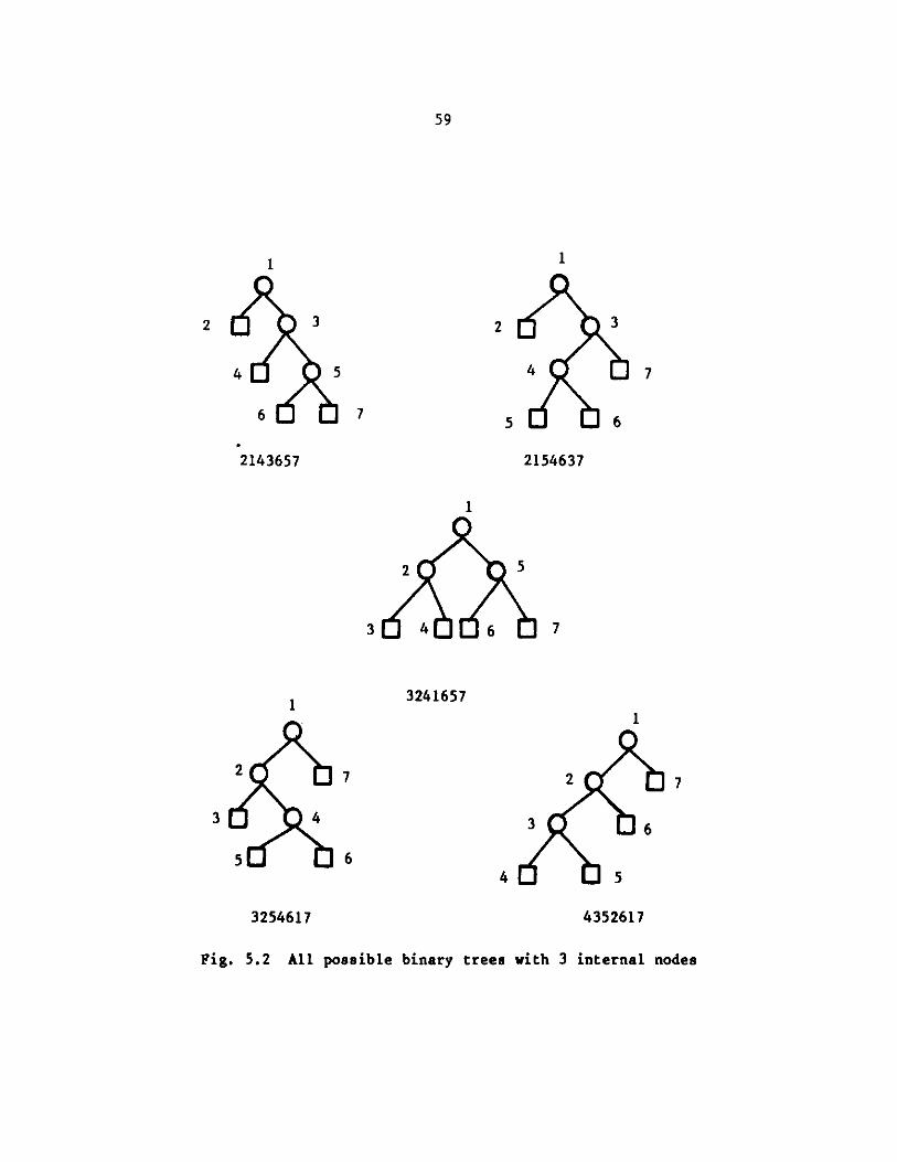
59

1

2 3

4 5

6 7

2143657

1

2 3

4 7

5 6

2154637

1

2 5

3 4 6 7

1

2 7

3 4

5 6

3241657

1

2 7

3 6

4 5

3254617 4352617

Fig. 5.2 All possible binary trees with 3 internal nodes

60

Possibility 2: All triples ak+li m, aj, j > k+2 are non-violating triples,but ai m aj' is a violating triple for some i < k+l and j > k+2. This canbe expressed as follows:

j, j > k+2, ak+l > aj > m (5.1)

and

3 i,j', i c k, j' > k+2, ai > aj' > m. (5.2)

Expression (5.1) can be rewritten as

Yj > k+2, ak+l 4 aj or_ aj < m. (5.3)

Of this, aj < m is always false, since m is the smallest element. Therefore,(5.3) becomes

Yj > k+2, ak+l < aj.

We can deduce

Yj > k+2, ak+l < aj, (5.4)

since the ai's are all distinct. From (5.2) it follows that for some i,j

i < k+l, j > k+l, ai > aj. (5.5)

Therefore, for the j satisfying (5.5),

ai > aj > ak+1,

which is a violating triple and hence contradicts the assumption that ala2... an is a g-stack permutation. Hence, 'possibility 2' does not exist. It

is enough if we check for 'possibility 1' in each of the permutationsgenerated by 'Migrate.' The condition expressed by 'possibility 1' is

% j,j > k+2, ak+l > aj > in.

The above condition is adequate to ensure that the extension is g-stack

permutation. Since m is the smallest element in the extension, aj > m is

guaranteed. Therefore it is enough if we check whether ak+l > aj for any

j > k+2. Since all the elements are distinct, the condition we have to check

reduces to

Yj > k+2, aj > ak+l.

This is precisely the condition that we will use in adapting the function'Migrate' to generate stack permutations. After adding this condition, we

obtain the definition of 'Spmigrate'

61

Spmigrate({<u,v>}) ( {<u,v>}

Sprigrate(F) < {F} U {{<st1>} U F2 0 1F2 0 c Sphop(t1 ,

{<s 1,t>,r})}

Sphop(w,{<u,v>}) < {{<u,v>}}

Sphop(w,F 2 1 ) < {{<s,t 1 >} U F2 2 1F2 2 e Sphop (t 1, {<s 1,t>,rI)}

if_' y E range(F2 1 -{<s,t>}) such that y < w

< {{(s,t1>} U F2 3jF2 3 e Sphop (t1, {<s1,t>,r})},

otherwise,

where s,t,s 1,t1,r are as defined in the beginning of Section 4.1.2. The

complete algorithm for generating stack permutations is given by

Spperm(0) <= 0

Spperm({<u,v>}) < {{<u,v>}}

Spperm(F) <= U Spmigrate(F2 4 )

F2 4c Spfixone(F,v1),

where v1 is as defined in (4.10).

Spfixone(F,v1) <_ {{<i,v1>} U F25 IF25 Spperm(F-{<i,v1>})}

where i - preimage(v1) in F.

Spmigrate({<u,v>}) ( {{<u,v>}}

Spmigrate(F) <_ {F} U {{<st1>} U F 2 0 1F2 0 c Sphop(t1 ,

{<s 1,t>,r})}

Sphop(w,{<u,v>} <_ {{<u,v>}}

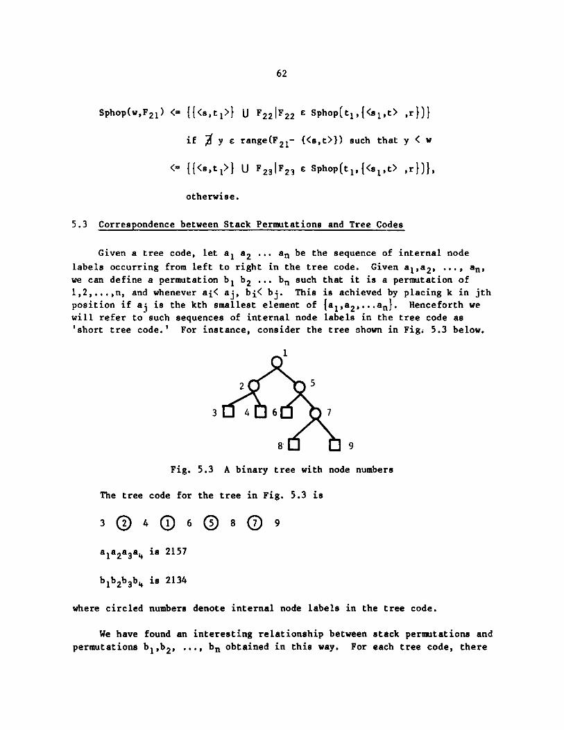
62

Sphop(w,F2 1) <_ {{<s,t1>} U F2 2 1F2 2 a Sphop(t1 ,(<s 1 ,t> ,r})}

if ' y e range(F2 1 - {<s,t>}) such that y < w

<= {{<s,tl>} U F2 31F2 3 a Sphop(t 1 ,{<s 1 ,t> ,r})),

otherwise.

5.3 Correspondence between Stack Permutations and Tree Codes

Given a tree code, let al a2 ... an be the sequence of internal node

labels occurring from left to right in the tree code. Given a1 ,a2, ... , an,we can define a permutation b1 b2 ... bn such that it is a permutation of1,2,... ,n, and whenever ai< aj, bi< bj. This is achieved by placing k in jthposition if aj is the kth smallest element of {ai,a2,...an}. Henceforth we

will refer to such sequences of internal node labels in the tree code as'short tree code.' For instance, consider the tree shown in Fig. 5.3 below.

2 5

3 4 6 7

8 9

Fig. 5.3 A binary tree with node numbers

The tree code for the tree in Fig. 5.3 is

3QO24 Q®6®OS8Q9 9

a1a2a3a4 is 2157

b1 b2b3 b4 is 2134

where circled numbers denote internal node labels in the tree code.

We have found an interesting relationship between stack permutations and

permutations b1,b2 , ... , bn obtained in this way. For each tree code, there

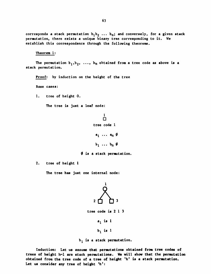
63

corresponds a stack permutation b1 b2 ... bn; and conversely, for a given stackpermutation, there exists a unique binary tree corresponding to it. Weestablish this correspondence through the following theorems.

Theorem 1:

The permutation b1,b2, ... , bn obtained from a tree code as above is a

stack permutation.

Proof: by induction on the height of the tree

Base cases:

1. tree of height 0.

The tree is just a leaf node:

1

tree code 1

a1 ... an 0

bi ... bn 0

0 is a stack permutation.

2. tree of height 1

The tree has just one internal node:

2 3

tree code is 2 1 3

a1 is 1

b1 is 1

bl is a stack permutation.

Induction: Let us assume that permutations obtained from tree codes oftrees of height h-1 are stack permutations. We will show that the permutationobtained from the tree code of a tree of height 'h' is a stack peratation.Let us consider any tree of height 'h':

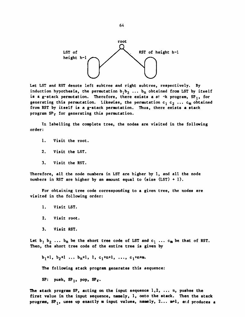
64

root

LST of RST of height h-1height h-i

Let LST and RST denote left subtree and right subtree, respectively. By

induction hypothesis, the permutation b1b2 ... bn obtained from LST by itselfis a g-stack permutation. Therefore, there exists a St ^k program, SP1, for

generating this permutation. Likewise, the permutation c1 c2 ... cm obtainedfrom RST by itself is a g-stack permutation. Thus, there exists a stack

program SPr for generating this permutation.

In labelling the complete tree, the nodes are visited in the following

order:

1. Visit the root.

2. Visit the LST.

3. Visit the RST.

Therefore, all the node numbers in LST are higher by 1, and all the nodenumbers in RST are higher by an amount equal to (size (LST) + 1).

For obtaining tree code corresponding to a given tree, the nodes are

visited in the following order:

1. Visit LST.

2. Visit root.

3. Visit RST.

Let b1 b2 ... bn be the short tree code of LST and cl ... cm be that of RST.Then, the short tree code of the entire tree is given by

b1+1, b2+1 ... bn+1, 1, c1+n+1, ... , c1+n+m.

The following stack program generates this sequence:

SP: push, SP1 , pop, SPr.

The stack program SP, acting on the input sequence 1,2, ... n, pushes the

first value in the input sequence, namely, 1, onto the stack. Then the stack

program, SP1, uses up exactly m input values, namely, 2... m+l, ard produces a

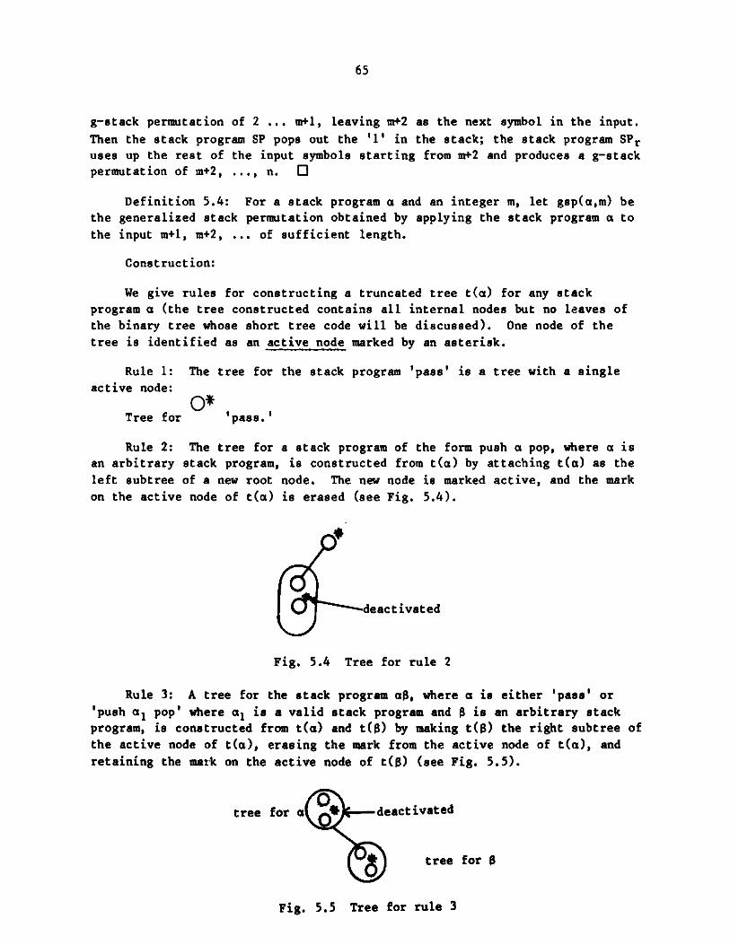
65

g-stack permutation of 2 ... m+l, leaving m+2 as the next symbol in the input.

Then the stack program SP pops out the '1' in the stack; the stack program SPruses up the rest of the input symbols starting from m+2 and produces a g-stack

permutation of m+2, ..., n. 0

Definition 5.4: For a stack program a and an integer m, let gsp(a,m) be

the generalized stack permutation obtained by applying the stack program a to

the input m+l, m+2, ... of sufficient length.

Construction:

We give rules for constructing a truncated tree t(a) for any stack

program a (the tree constructed contains all internal nodes but no leaves of

the binary tree whose short tree code will be discussed). One node of thetree is identified as an active node marked by an asterisk.

Rule 1: The tree for the stack program 'pass' is a tree with a singleactive node:

0*Tree for 'pass.'

Rule 2: The tree for a stack program of the form push a pop, where a is

an arbitrary stack program, is constructed from t(a) by attaching t(a) as the

left subtree of a new root node. The new node is marked active, and the mark

on the active node of t(a) is erased (see Fig. 5.4).

deactivated

Fig. 5.4 Tree for rule 2

Rule 3: A tree for the stack program aB, where a is either 'pass' or

'push ai pop' where a1 is a valid stack program and S is an arbitrary stack

program, is constructed from t(a) and t(8) by making t(B) the right subtree of

the active node of t(a), erasing the mark from the active node of t(a), and

retaining the mark on the active node of t(8) (see Fig. 5.5).

0tree for a deactivated

tree for 0

Fig. 5.5 Tree for rule 3

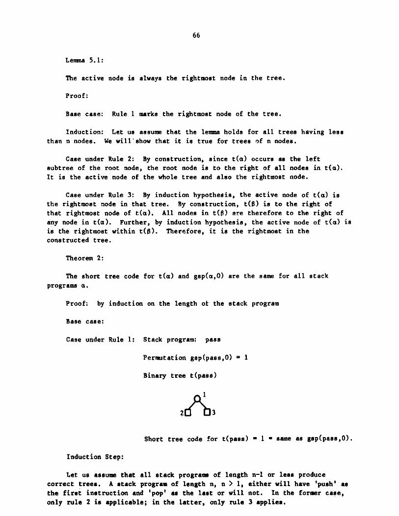
66

Lemma 5.1:

The active node is always the rightmost node in the tree.

Proof:

Base case: Rule 1 marks the rightmost node of the tree.

Induction: Let us assume that the lemma holds for all trees having less

than n nodes. We will'show that it is true for trees of n nodes.

Case under Rule 2: By construction, since t(a) occurs as the leftsubtree of the root node, the root node is to the right of all nodes in t(a).

It is the active node of the whole tree and also the rightmost node.

Case under Rule 3: By induction hypothesis, the active node of t(a) isthe rightmost node in that tree. By construction, t(O) is to the right ofthat rightmost node of t(a). All nodes in t(0) are therefore to the right of

any node in t(a). Further, by induction hypothesis, the active node of t(a) is

is the rightmost within t(S). Therefore, it is the rightmost in theconstructed tree.

Theorem 2:

The short tree code for t(a) and gsp(a,0) are the same for all stack

programs a.

Proof: by induction on the length of the stack program

Base case:

Case under Rule 1: Stack program: pass

Permutation gsp(pass,0) - 1

Binary tree t(pass)

2 3

Short tree code for t(pass) - 1 ' same as gsp(pasa,0).

Induction Step:

Let us assume that all stack programs of length n-1 or less producecorrect trees. A stack program of length n, n > 1, either will have 'push' asthe first instruction and 'pop' as the last or will not. In the former case,

only rule 2 is applicable; in the latter, only rule 3 applies.

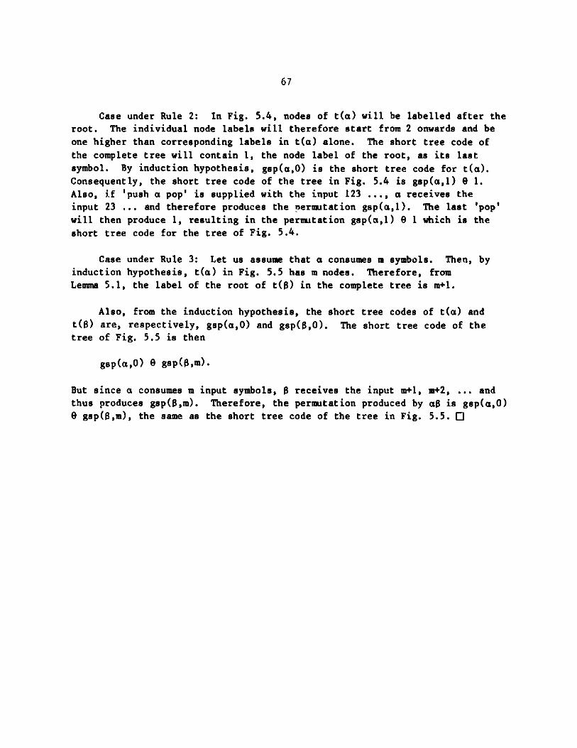
67

Case under Rule 2: In Fig. 5.4, nodes of t(a) will be labelled after theroot. The individual node labels will therefore start from 2 onwards and be

one higher than corresponding labels in t(a) alone. The short tree code ofthe complete tree will contain 1, the node label of the root, as its lastsymbol. By induction hypothesis, gsp(a,0) is the short tree code for t(a).Consequently, the short tree code of the tree in Fig. 5.4 is gap(a,1) 9 1.Also, if 'push a pop' is supplied with the input 123 ... , a receives theinput 23 ... and therefore produces the nermutation gsp(a,1). The last 'pop'will then produce 1, resulting in the permutation gsp(a,1) 9 1 which is the

short tree code for the tree of Fig. 5.4.

Case under Rule 3: Let us assume that a consumes m symbols. Then, byinduction hypothesis, t(a) in Fig. 5.5 has m nodes. Therefore, fromLemma 5.1, the label of the root of t(O) in the complete tree is m+1.

Also, from the induction hypothesis, the short tree codes of t(a) andt(s) are, respectively, gsp(a,O) and gsp(B,0). The short tree code of thetree of Fig. 5.5 is then

gsp(a,0) e gsp(R,m).

But since a consumes m input symbols, B receives the input m+1, m+2, ... andthus produces gsp(B,m). Therefore, the permutation produced by aB is gsp(a,0)e gap(B,m), the same as the short tree code of the tree in Fig. 5.5. 0

68

CHAPTER 6

CONCLUSION

We have presented a methodology for algorithm development through schematransformations. This methodology features a natural integration between thedevelopments of algorithms and their proofs. The many algorithms that getdeveloped for a problem fit into a systematic structure that is often amenableto extension at each of the branch points. The commonalities between variousalgorithms can aid in collective proof development.

In Chapter 4, we have suggested 16 permutation algorithms. The number can

be easily increased further, for example, by finding more alternative ways ofcombining the last element with the permutations of the remaining elements.However, there are permutation algorithms that are unlikely to be generatedthrough the extension of this structure (see, for example, Ref. 35).

The development in Chapter 5 gives one instance of an application of thestructure in Chapter 4 to a related but different programming problem, which isan aspect of programming which could stand more study. The correspondence wehave shown between stack permutations and binary trees could be exploited to

further adapt the stack permutation algorithm for the generation of binarytrees.

The style of collective development of related algorithms needs more ex-ploration to find out all the ways in which it can be used in programming. Italso has repercussions on the teaching of programming.

Further work in the area can try to generalize as much as possible thesystems of transformations available to the programmer. The system we have

described in Chapter 3 is suited for set-theoretic problems. One can eitherseek common transformation rules that are applicable to a number of problemdomains or compile rules that cover, individually, a number of domains. Withthe extension of the scope of available rules one can examine diverse program-ming problems with a view to discovering the recurring paradigms of this style.Together with this exercise one could build computer support for the methodol-ogy in the form of algorithm schema manipulation tools and possibly cataloguingsystems.

69

ACKNOWLEDGMENTS

I am deeply grateful to the following people:

Professor R. V. Sahasrabuddhe, my thesis supervisor, for his insight,enthusiasm,and patience. Without his encouragement and support I could nothave brought this work to completion.

Dr. James M. Boyle and Dr. Paul Messina, for their encouragement andsupport in bringing out thi' report.

Mr. H. Karnick, for the help in debugging the LISP programs.

Dr. Gail Pieper, for helping me in the proofreading.

All my friends who made my stay at Kanpur memorable.

70

REFERENCES

1. F. E. Allen and J. Cocke, "A Catalogue of Optimising Transformations," in

Design and Optimisation of Compilers, R. Rustin, ed., Prentice-Hall (1972),pp. 1-30.

2. R. Balzer, N. Goldman, and D. Wile, "On the Transformational Approach to

Programming," in Proc. Second Internationc 1 Conference on Software Engi-neering, San Francisco (1976), pp. 337-344.

3. R. Balzer, N. Goldman, and D. Wile, Informlity in Progam Specifications,IEEE Trans. on Software Engineering, SE-4(2), 94-103 (1978).

4. D. R. Barstow, An Experiment in Knowledge-based Programming, ArtificialIntelligence 12, 73-119 (1979).

5. D. R. Barstow, Knowledge-Based Program Construction, North Holland (1979).

6. L. Beckman et al., A Partial Evaluator and Its Use as a Programming Toot,Artificial Intelligence 7, 319-357 (1976).

7. A. W. Biermann, "Approaches to Automatic Programming," in Advances in

Computers, M. Rabinoff and M. C. Yovits, eds., vol. 15, Academic Press,

New York (1976), pp. 11-63.

8. R. M. Burstall and J. Darlington, A Transformation System for DevelopingRecursive Programs, Journal of the ACM 24(1), 44-67 (1977).

9. J. Darlington, A Synthesis of Several Sorting Algorithms, ACTA Infor-matica 11, 1-30 (1978).

10. J. Darlington and R. M. Burstall, A System Which Automatically ImprovesPrograms, ACTA Informatica 6, 41-60 (1976).

11. E. W. Dijkstra, A Discipline of Programming, Prentice-Hall (1976).

12. E. W. Dijkstra, "Notes on Structured Programming," in Structured Progmm-

ming, 0. S. Dahl, E. W. Dijkstra, and C. A. R. Hoare, eds., Academic PresNew York (1972), pp. 1-81.

13. R. W. Floyd, "Assigning Meanings to Programs," in Proc. Amer. Math. Soc.

Symposia in Applied :'athematics, vol. 19 (1967), pp. 19-31.

14. S. L. Gerhart and L. Yelowitz, Control Structure Abstractions of theBacktracking Programming Technique, IEEE Trans. on Software Engineering,SE-2(4), 285-292 (1976).

15. C. Green, "The Design of the PSI Program Synthesis System," in Proc.

Second International Conference on Softwmare Engineering, San Francisco(1976), pp. 4-18.

16. C. Green, "A Summary of the PSI Program Synthesis System," in Proc. of FifthInternational Conference on Artificial Intelligence, Cambridge, Massachusetts(1977), pp. 380-381.

71

17. C. Green and D. R. Barstow, On Program Synthesis Knowledge, Artificial

Intelligence 10, 241-279 (1978).

18. A. Haraldson, A Partial Evaluator and Its Use for Compiling IterativeStatements in LISP, LiTH-MAT-R-77-26, Linkoeping University (1977).

19. A. Haraldson, A Program Manipulation System Based on Partial Evaluation,Ph.D. Thesis, Linkoeping University, Sweden (1977).

20. C. A. R. Hoare, An Axiomntic Basis for Computer Programming, Commun.ACM 12, 576-580 (1969).

21. C. A. R. Hoare, "Notes on Data Structuring," in Structured Programming,

0. J. Dahl, E. W. Dijkstra, and C. A. R. Hoare, eds., Academic Press,

New York (1972), pp. 83-174.

22. C. A. R. Hoare, Proof of Correctness of Data Representations, ACTA Infor-matica 1(4), 271-281 (1972).

23. D. F. Kibler, Power, Efficiency and Correctness of Transformtion Systems,Ph.D. Thesis, Computer Science Dept., University of California at Irvine

(1978).

24. G. D. Knott, A Numbering System for Binary Trees, Commun. ACM 20(2),113-115 (1977).

25. D. E. Knuth, The Art of Computer Programning, vol. 1: FundamentalAlgorithms, Addison-Wesley Pub. Co, Reading, Massachusetts (1973).

26. D. E. Knuth, The Art of Computer Programnning, vol. 3: Sorting andSearching, Addison-Wesley Pub. Co., Reading, Massachusetts (1973).

27. D. E. Knuth, Structured Programmning with Go To Statements, ComputingSurveys 6(4), 261-302 (1974).

28. B. W. Lampson et al., Report on the Programming Language Euclid, ACMSIGPLAN Notices 12(2), pp. 1-79 (1977).

29. B. H. Liskov and S. N. Zilles, Specification Techniques for Data Abstrac-tions, IEEE Trans. on Software Engineering, vol. SE-1(1), 7-19 (1975).

30. B. H. Liskov et al., Abstraction Mechanisms in CLU, Commun. ACM 20(8),564-576 (1977).

31. D. B. Loveman, Program Improvement by Source-to-Source Traneformations,Journal of the ACM 24, 121-145 (1977).

32. Z. Manna and R. Waldinger, The Logic of Computer Prograning, IEEE Trans.on Software Engineering, vol. SE-4(3), 199-229 (1978).

33. Z. Manna and R. Waldinger, Synthesis: Dreams => Programs, IEEE Trans. on

Software Engineering, vol. SE-5(4), 294-328 (1979).

34. P. B. Schneck and E. Angel, FORTR4N to FORTRAN Optimising Compiler, Com-puter Journal 16(4), 322-340 (1973).

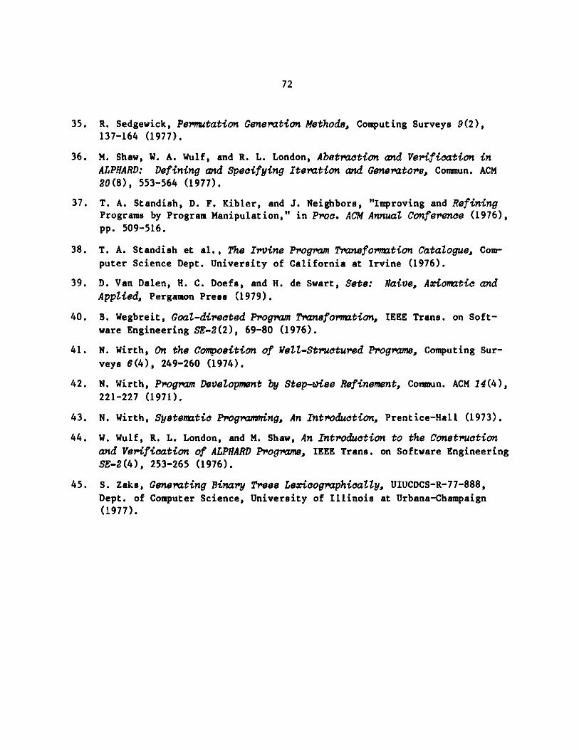
72

35. R. Sedgewick, Permutation Generation Methods, Computing Surveys 9(2),137-164 (1977).

36. M. Shaw, W. A. Wulf, and R. L. London, Abstraction and Verification inALPHARD: Defining and Specifying Iteration and Generators, Commun. ACM20(8), 553-564 (1977).

37. T. A. Standish, D. F. Kibler, and J. Neighbors, "Improving and RefiningPrograms by Program Manipulation," in Proc. ACM Annual Conference (1976),pp. 509-516.

38. T. A. Standish et al., The Irvine Program Traneformation Catalogue, Com-puter Science Dept. University of California at Irvine (1976).

39. D. Van Dalen, H. C. Doefs, and H. de Swart, Sets: Naive, Axiomatic andApplied, Pergamon Press (1979).

40. B. Wegbreit, Goal-directed Program Transfornrrtion, IEEE Trans. on Soft-ware Engineering SE-2(2), 69-80 (1976).

41. N. Wirth, On the Composition of Wetl-Structured Programs, Computing Sur-veys 6(4), 249-260 (1974).

42. N. Wirth, Program Development by Step-wise Refinement, Conmun. ACM 14(4),221-227 (1971).

43. N. Wirth, Systemtic Programing, An Introduction, Prentice-Hall (1973).

44. W. Wulf, R. L. London, and M. Shaw, An Introduction to the Constructionand Verification of ALPRARD Programs, IEEE Trans. on Software EngineeringSE-2(4), 253-265 (1976).

45. S. Zaks, Generating Binary Trees Lexicographically, UIUCDCS-R-77-888,Dept. of Computer Science, University of Illinois at Urbana-Champaign

(1977).

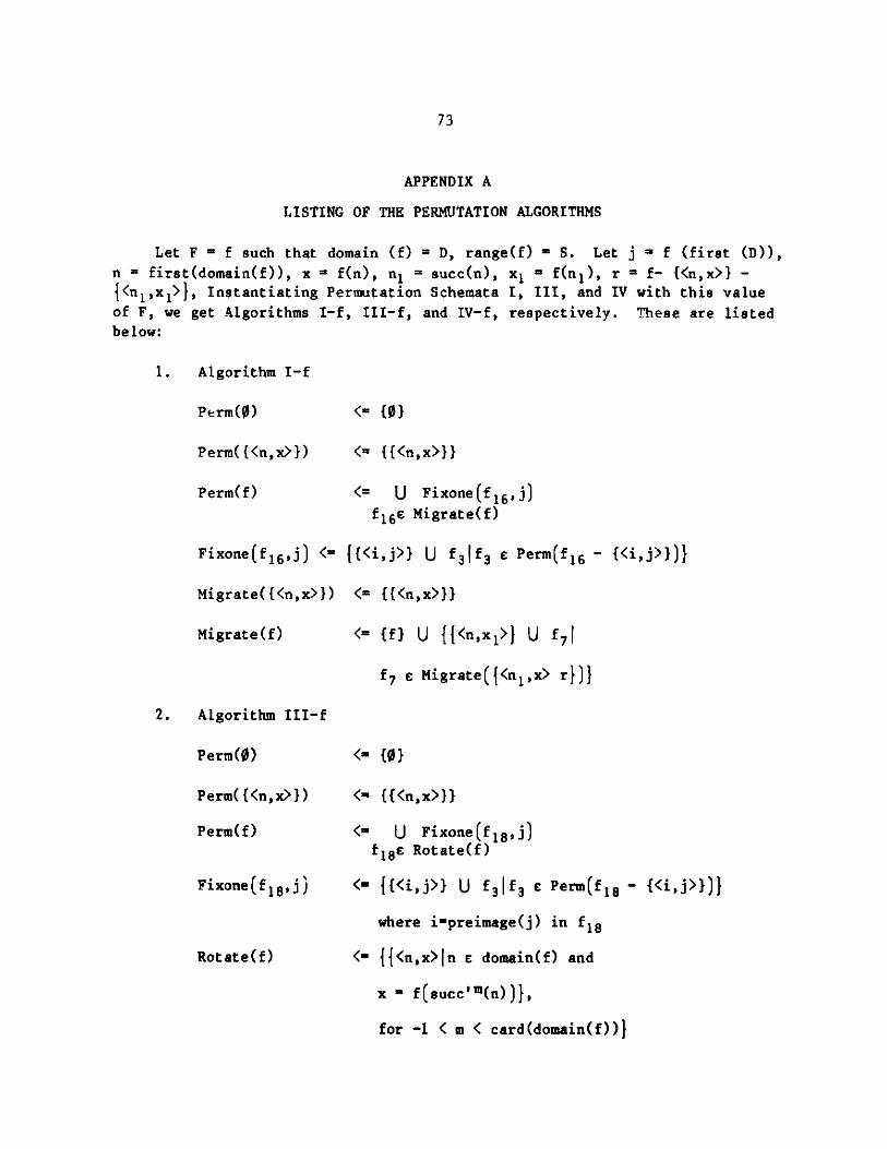
73

APPENDIX A

LISTING OF THE PERMUTATION ALGORITHMS

Let F = f such that domain (f) = D, range(f) = S. Let j f (first (D)),n = first(domain(f)), x = f(n), n1 = succ(n), xi = f(ni), r = f- {<n,x>} -{<ni,xi>}, Instantiating Permutation Schemata I, III, and IV with this valueof F, we get Algorithms I-f, III-f, and IV-f, respectively. These are listedbelow:

1. Algorithm I-f

Perm(0) <= 01

Perm({<n,x>})

Perm(ff)

<= {{<n,x>}}

<= U Fixone(fl6,,j)

f16e Migrate(f)

Fixone(f16 ,j) <- {{<i,j>} U f3 1f 3 e Perm(f16 - {<i,j>})}

Migrate({<n,x>})

Migrate(f)

<= ({<n,x>}}

<= {f} U {{<n,xl>} U f7j

f7 c Migrate({<n1 ,x> r))

2. Algorithm III-f

Perm(0) <- {}

Perm({<n,x>})

Perm(f)

Fixone(f1 8,j)

Rotate(f)

<= {{<n,x>}}

<- U Fixone(fl 8 ,j)118E Rotate(f)

<- {{<i,j>} U f3lf3 c Perm(f1 8 - {<i,j>})}

where impreimage(j) in f18

< {{<n,x>jn domain(f) and

x - f(succ'm(n))},

for -1 < m < card(domain(f))}

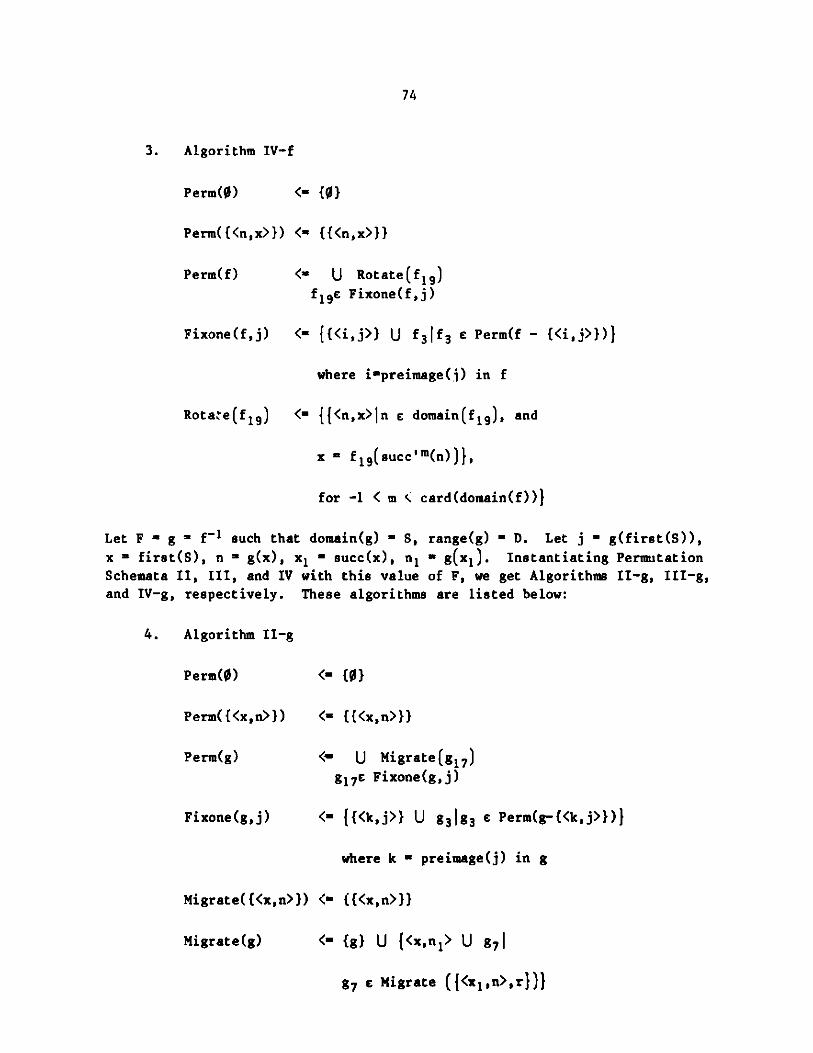
74

3. Algorithm IV-f

Perm(0) (a {}

Perm({<n,x>}) <= {{<n,x>}}

<U U Rotate(f1 9 )

f19e Fixone(f,j)

Fixone(f,j) < {{<i,j>} U f 3 jf3 Perm(f - {<i,j>})}

where impreimage(j) in f

Rota;e(f 1 9 ) <( {{<n,x>jn e domain(f19 ), and

x = f 19 (succsm(n))I,

for -1 < m < card(domain(f))}

Let F = g = f 1 such that domain(g) - S, range(g) - D. Let j - g(first(S)),x = first(S), n - g(x), x1 - succ(x), n1 - g(x1 ). Instantiating Permutation

Schemata II, III, and IV with this value of F, we get Algorithms II-g, III-g,and IV-g, respectively. These algorithms are listed below:

4. Algorithm II-g

Perm(0) <- (0}

Perm({<x,n>})

Perm(g)

Fixone(g,j)

<= ((<x,n>}}

<w U Migrate(g1 7 )gl 7e Fixone(g,j)

<= {{<k,j>} U g31g3 e Perm(g-(<k,j>})}

where k - preimage(j) in g

Migrate((<x,n>}) <" {{<x,n>}}

Migrate(g) <{ (g} U {<x,n1 > U g71

g7 c Migrate ({<x 1 ,n>,r})I

Perm(ff)

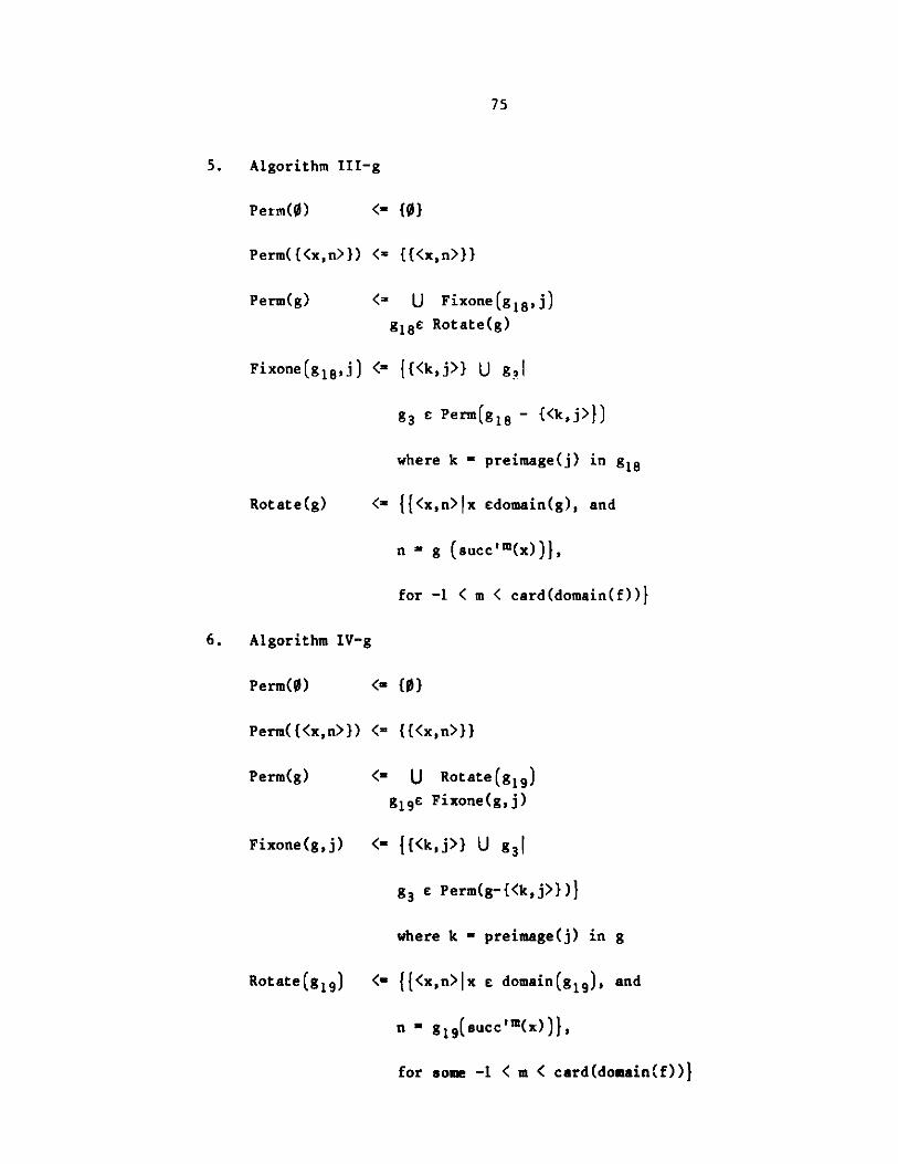
75

5. Algorithm III-g

Perm(O) < {0}

Perm({<x,n>}) < {{<x,n>J}

Perm(g) <= U Fixone(g18,j)

g1 8e Rotate(g)

Fixone(g1 8,j) <= {{<k,j>} U g.41

g3 c Perm(g1 8 - {<k,j>})

where k - preimage(j) in g18

Rotate(g) <_ {{<x,n>jx edomain(g), and

n = g (succ'm(x))},

for -1 < m < card(domain(f))}

6. Algorithm IV-g

Perm(O) <_ {0}

Perm({<x,n>}) <= {{<x,n>}}

Perm(g) <- U Rotate(g19 )

g19e Fixone(g,j)

Fixone(g,j) <_ {{<k,j>} U g31

g3 cPerm(g-{<k,j>})}

where k - preimage(j) in g

Rotate(g1 9) <_ {{<x,n>Ix c domain(g19), and

n - g19(succ'm(x))},

for some -1 < m < card(domain(f))}

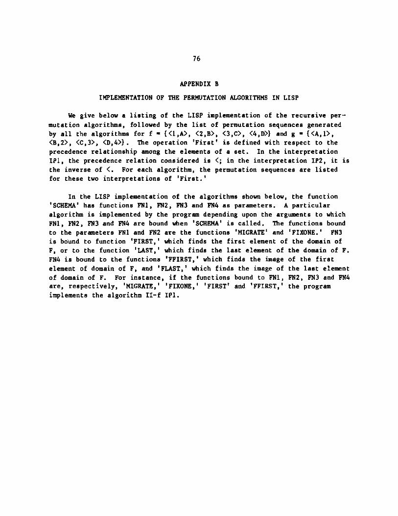
76

APPENDIX B

IMPLEMENTATION OF THE PERMUTATION ALGORITHMS IN LISP

We give below a listing of the LISP implementation of the recursive per-mutation algorithms, followed by the list of permutation sequences generatedby all the algorithms for f - {<1,A>, <2,B>, <3,C>, <4,D>} and g - {<A,1>,<B,2>, <C,3>, <D,4>}. The operation 'First' is defined with respect to theprecedence relationship among the elements of a set. In the interpretationIP1, the precedence relation considered is (; in the interpretation IP2, it isthe inverse of <. For each algorithm, the permutation sequences are listedfor these two interpretations of 'First.'

In the LISP implementation of the algorithms shown below, the function'SCHEMA' has functions FN1, FN2, FN3 and FN4 as parameters. A particularalgorithm is implemented by the program depending upon the arguments to whichFN1, FN2, FN3 and FN4 are bound when 'SCHEMA' is called. The functions boundto the parameters FN1 and FN2 are the functions 'MIGRATE' and 'FIXONE.' FN3is bound to function 'FIRST,' which finds the first element of the domain ofF, or to the function 'LAST,' which finds the last element of the domain of F.FN4 is bound to the functions 'FFIRST,' which finds the image of the first

element of domain of F, and 'FLAST,' which finds the image of the last elementof domain of F. For instance, if the functions bound to FN1, FN2, FN3 and FN4are, respectively, 'MIGRATE,' 'FIXONE,' 'FIRST' and 'FFIRST,' the program

implements the algorithm II-f IPi.

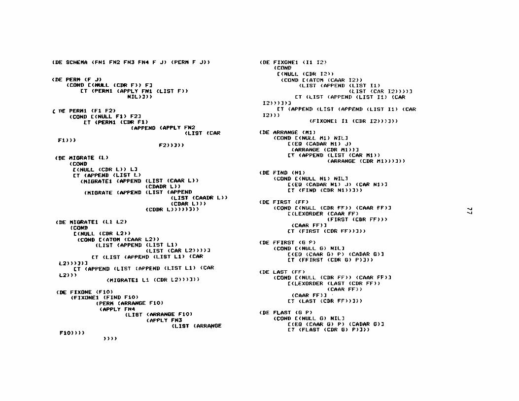
(DE SCHEMA (FN1 FN2 FN3 FN4 F J) (PERM F J))

(DE PERM (F J)CONDOD ((NULL (CDR F)) FJ

CT (PERM1 (APPLY FN1 (LIST F))NIL)]))

D tE PERM1 (Fl F2)(COND ((NULL Fl) F2J

CT (PERM1 (CDR Fl)(APPEND (APPLY FN2

(LIST (CAR

Fl)))F2))]))

(DE MIGRATE (L)CONDOD((NULL (CDR L)) L)CT (APPEND (LIST L)

(MIGRATEl (APPEND

(MIGRATE (APPEND

(LIST (CAAR L))(CD'ADR L))(LIST (APPEND

(LIST (CAADR L))(CDAR L)))

(CDDR L)))))]))

(DE MIGRATED (LI L2)CONDOD((NULL (CDR L2))CONDOD ((ATOM (CAAR L2))

(LIST (APPEND (LIST L1)(LIST (CAR L2))))]

ET (LIST (APPEND (LIST L1) (CAR

L2) ) )])]JET (APPEND (LIST (APPEND (LIST L1) (CAR

L2)))MIGRATEDI L1 (CDR L2)))]))

(DE FIXONE (FiO)(FIXONEI (FIND FiO)

(PERM (ARRANGE FiO)(APPLY FN4

(LIST (ARRANGE FiO)(APPLY FN3

(LIST (ARRANGE

F10))))

(DE FIXONE1 (I1I2)(CONE'((NULL (CDR 12))(CONK ((ATOM (CAAR 12))

(LIST (APPEND (LIST II)(LIST (CAR 12))))]IT (LIST (APPEND (LIST Ii) (CAR

I2)))])CT (APPEND (LIST (APPEND (LIST I1) (CAR

12)))(FIXONEl I1 (CDR 12)))]))

(DE ARRANGE (Ml)CONDOD [(NULL Ml) NIL)

C(EQ (CADAR Ml) J)(ARRANGE (CDR Mi)))ET (APPEND (LIST (CAR Ml))

(ARRANGE (CDR Mi)))]))

(DE FIND (Ni)(CONE' ((NULL Ni) NIL)

(C(EQ (CADAR Ni) J) (CAR Ni))IT (FIND (CDR Ni))]))

(DE FIRST (FF)(CONK ((NULL (CDR FF)) (CAAR FF)J

((LEXORDER (CAAR FF)(FIRST (CDR FF)))

(CAAR FF))CT (FIRST (CER FF))]))

(DE FFIRST (G P)(CONE' ((NULL G) NIL)

((EQ (CAAR G) P) (CADAR G))CT (FFIRST (CDR G) P)))

(DE LAST (FF)CONDOD ((NULL (CDR FF)) (CAAR FF))

C(LEXORDER (LAST (CDR FF))(CAAR FF))

(CAAR FF))CT (LAST (CDR FF))]))

(DE FLAST (G P)(CON ((NULL G) NIL)

((EQ (CAAR G) P) (CADAR G))(T (FLAST (CER G) P)]))

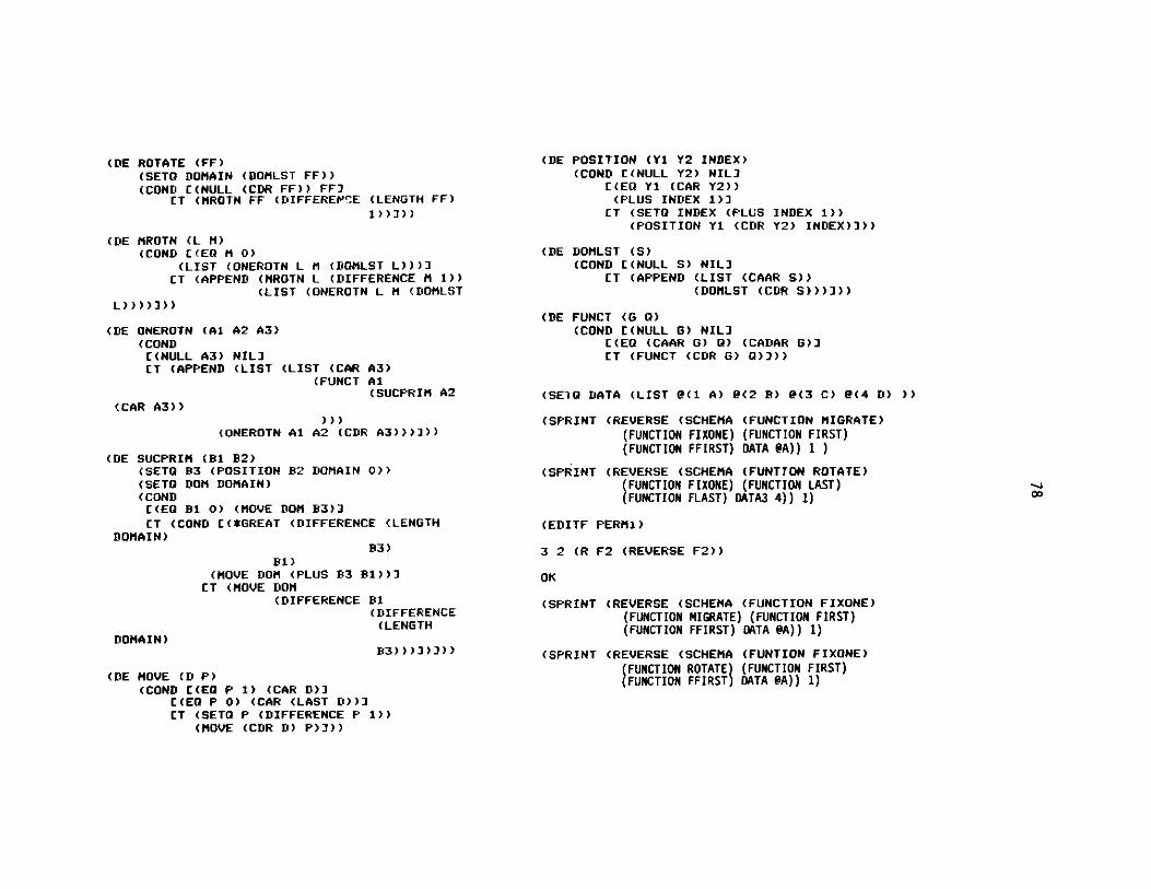
(DE ROTATE (FF)(SETO DOMAIN (DOMLST FF))(COND ((NULL (CDR FF)) FFJ

CT (MROTN FF DIFFERENCEE (LENGTH FF)1))]))

(DE MROTN (L M)(COND C(EQ M 0)

(LIST (ONEROTN L M (DOMLST L)))J(T (APPEND (MROTN L (DIFFERENCE M 1))

(LIST (ONEROTN L M (DOMLSTL))))]J))

(DE ONEROTN (Al A2 A3)(COND((NULL A3) NIL)CT (APPEND (LIST (LIST (CAR A3)

(FUNCT Al(SUCPRIM A2

(CAR A3)))))

(ONEROTN Al A2 (CDR A3)))J))

(DE SUCPRIM (B1 B2)(SETO B3 (POSITION B2 DOMAIN 0))(SETO DOM DOMAIN)(CONDC(EQ B1 0) (MOVE DOM B3))

CT (COND C(*GREAT (DIFFERENCE (LENGTHDOMAIN)

B3)B1)

(MOVE DOM (PLUS B3 B1))]CT (MOVE DOM

(DIFFERENCE B1(DIFFERENCE(LENGTH

DOMAIN)B3)))J)J))

(DE MOVE (D P)(COND C(EQ P 1) (CAR D)J

C(EQ P 0) (CAR (LAST D))JCT (SETA P (DIFFERENCE P 1))

(MOVE (CDR D) P)]))

(DE POSITION (Y1 Y2 INDEX)(COND [(NULL Y2) NIL)

C(EQ Y1 (CAR Y2))(PLUS INDEX 1)]

CT (SETQ INDEX (PLUS INDEX 1))(POSITION Y1 (CDR Y2) INDEX)]))

(DE DOMLST (S)(COND [(NULL S) NIL)

CT (APPEND (LIST (CAAR S))(DOMLST (CDR S)))]))

(DE FUNCT (G 0)(COND [(NULL 6) NIL)

((EQ (CAAR G) 0) (CADAR 6))CT (FUNCT (CDR G) 0)]))

(SElQ DATA (LIST @(1 A) @(2 B) @(3 C) l(4 D) ))

(SPRINT (REVERSE (SCHEMA (FUNCTION MIGRATE)(FUNCTION FIXONE) (FUNCTION FIRST)(FUNCTION FFIRST) DATA @A)) 1

(SPRINT (REVERSE (SCHEMA (FUNTTON ROTATE)(FUNCTION FIXONE) (FUNCTION LAST)(FUNCTION FLAST) DATA3 4)) 1)

(EDITF PERM1)

3 2 (R F2 (REVERSE F2))

OK

(SPRINT (REVERSE (SCHEMA (FUNCTION FIXONE)(FUNCTION MIGRATE) (FUNCTION FIRST)(FUNCTION FFIRST) DATA @A)) 1)

(SPRINT (REVERSE (SCHEMA (FUNTION FIXONE)

FUNCTION ROTATE (FUNCTION FIRST)FUNCTION FFIRST DATA @A)) 1)

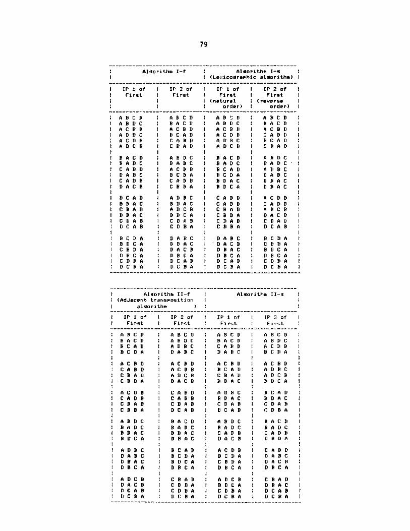
79

Algorithm I-f Algorithm I-gI (Lexicographic algorithm)

IP i of IP 2 of IFlI of I IP 2 ofFirst I First First I First

(natural (reverseorder) order)

A B C D I A B C D I A B C D A B C DA B D C I B A C D I A B D C 1 B A C DA C B D A C B D I A C DD A C B DA D B C C A D A C D B I C A B DA C D B C A B D A D B C I B C A DA D C B I C B A D I A D C B I C B A D

B A C D I A B D C B A C D A B D CSA D C I B A D C B A D C B A D CC A B D I A C D B I B C A D I A D B CD A B C B C D A I B C D A D A B C1

C A D B C A D B I B D AC I B D A CD A C B I C B D A I B D C A I D BRA C

R C A D I A D B C I C A BD A C D BB D A C I B D A C I C A DB I C A D BC B A D ! A D C B I C R A D I A D C BD B A C I B D C A I C B D A D A C BC D A B I C D AB C D A B I C D A BD C A B C D B A I C D B A D C A B

B C D A D A B C I D A B C I B C D AB D C A I D B A C D A C B I C B D AC B D A I D A C B I D B A C B D C AD BRC A I DBC A I D BCA I D BC AC D B A[ D C A B D C A B I C D B AD C B A I D C B A D C B A I D C B A

Algorithm II-f I Algorithm II-1(AdJacent transposition

algorithm )

IP1 of I IP 2 of I IP1 of IP 2 ofFirst I First I First First

A BC D I AB C D I A BC D I A B CDB A C D IA B D C AUD I A B D CB C A D A D B C C A BRD I A C D BB C D A D A B C D A B C B C D A

A C B D I A C B D I A C B D I A C BDC A B D A C D B B C A D I A D B CC B A D A D C? iC R A DI A D C BC B D A D A C B I D B A C B D C A

A C D B I C A UB D A D B C B C A DC A D B I C A DB I BD AC I B D A CC D A B C D A B C D A B C D A BC D B A DAB D C A B C D B A

A BRD CIAD I A B D C I B A C DB A D C 1 B A D C I B A D C 1 B A D C

B D A C I B D A C C A D B I C A D BB D C A I DIBCAC I D A UCB I CU B [' A

D A B C I BC D A I BCDA I DBABCDIBA C I B DUCA I CUBD A D AC tDIBC A D BCA I D BC A : D BUCA

A DUCB I CUBAD I A DUCB UCB A D

D C A B I C D B A I C D B A I D C A BD C B A I D C B A I D C B A I D C B A

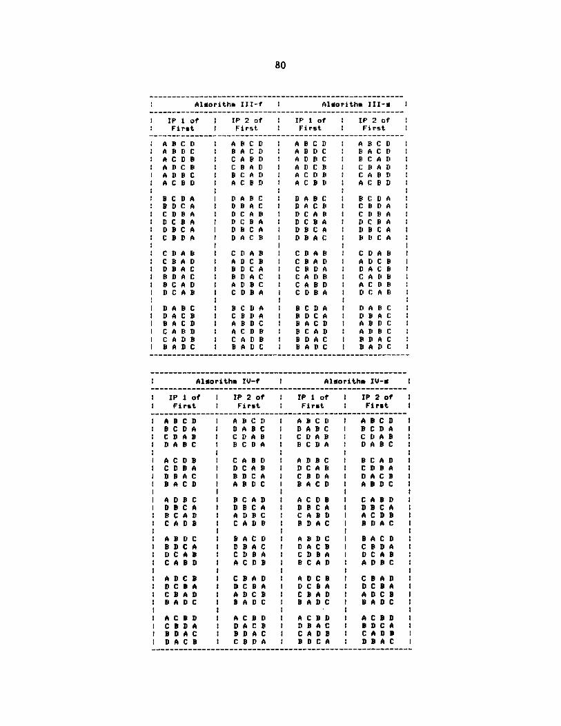
80

Algorithm III-f Algorithm III-

IP1 of 2 IP 2 of IP1 of 1 IP 2 ofFirst 2 First 1 First 2 First

A B C D A B C D I A B C D A B C DA B D C I D A C D I A B D C I R A C DA C D B C A [D 2 A D C B C A D 2A D C 2 IC R A D I A D C B CAA DA D B C B C A D I A C D R I C A R D

A C D 2 A C D A C D A C B D

S C D A 2 D A C 2 D A B C I 2 C D AB D C A D B A C D A C B C B D AC D B A I D C A B D C A I C D B AD C B A D C B A D C B A D C B AD B C A D B C A D B C A D B C AC B D A D A C B D B A C R D C A

C D A B I C D A BI C D A B I C D A BC B A D I A D C B C A D 2 A D C BD B A C D C A C B D A D A C BB D A C I B D A C C A D B 2 C A D B2 C A D A D B C C A D A C DD C A B I C D B A I C D B A D C A

D A B C II 2 C D A 2 I C D A I D A R CD A C B C B D A D C A D B A CB A C D A B D C A C D A B D CC A B D I A C D 2I B C A D A D R CIC A D B C A D B B D A C I B D A CR A D C I B A D C B A D C B A D C

Algorithm IV- I Algorithm IV-i

2 IP1of 2 IP 2of 2 IPIof IP 2 ofFirst 2 First 2 First 2 First I

A B C D I A B C D A B C D A B C D IB C D A D A B C I D A B C I C D AC D A B C D A B I C D A B I C D A BD A B C I R C D A I 2 C D A I D A B C

A C D B C AID 2 A D C I B C A D 2C D B A D C A B D C A B I C D B AD B A C I B D C A C B D A I D A C BIR A C D I A B D C I A C D A B D C

2 I I !A D B C I B C A D A C D B C A DD B C A D B C A I D B C A I D B C AB C A D 2 A D C 2 C A ID I A C D B !C A D B I C A D B 1 B D A C I B D A C2 CA I CA I 2IDC 2 DA

A B D C R A C D A B D C I R A C D

B D C A D B A C I D A C B I C B D AD C A B I C D B A C D B A I D C A BC A R D I A C D B B C A D I A D R C I

A D C D C AD I A D C B I C B A DD C B A I D C B A I D C B A D C B AC B A D 1 A D C B I C B A D I A D C B IB A D C I B A D C I B A D C I B A D C

A C A D I A C B D I A C B D I A C IDC CI D A D A C B I D B A C 1 2 D C A IB D A C I B D A C I C A D B I C A D B ID A C B I C B D A 1 2 D C A I D B A C I