Evaluating Bank Specialness

Juliane Begenau and Erik Stafford*

September 2017

ABSTRACT

Bank specialness combines notions of important economic functions, distinctive production technologies, and relative efficiency. We argue that direct evidence on the efficiency of distinctive bank technologies relative to those employed elsewhere in the capital market is scarce, but widely assumed to be supportive of the relative efficiency of banks. In contrast to this assumption, we find that, in the aggregate, (1) bank assets underperform passive portfolios of maturity-matched US Treasury bonds, (2) the cost of bank deposits exceeds the cost of bank debt, and (3) portfolios of bank equities consistently underperform portfolios designed to passively mimic their economic exposures over the period 1980 through 2015. The very strong investment performance of passive maturity transformation strategies over this period masks the underperformance of the specialized bank activities.

* Begenau (begenau@stanford.edu) and Stafford (estafford@hbs.edu) are at Stanford and Harvard Business School. We thank Robin Greenwood, Sam Hanson, David Scharfstein, Andrei Shleifer, Jeremy Stein, and Adi Sunderam for helpful comments and discussions. Harvard Business School’s Division of Research provided research support.

USC FBE FINANCE SEMINARpresented by Erik StaffordFRIDAY, Nov. 3, 201710:30 am – 12:00 pm, Room: JFF-236

1

Banks are widely viewed to be special. The notion that banks are special connotes that

their activities (1) are economically important, (2) rely on specific technologies that are distinct

from those used elsewhere in the capital market, and (3) are advantaged in the sense of allowing

for either lower production costs or improved investment returns than are available with

alternative capital market technologies. For example, Diamond (1984) develops a theory of

banking relying on banks having a net cost advantage in loan monitoring relative to the capital

market, providing banks a relative advantage in the credit issuance activity for many borrowers.

Diamond and Dybvig (1983) present a model of banks as liquidity providers with a production

technology that offers a relative advantage over capital markets in transforming illiquid assets

into short-term demandable claims. Gorton and Pennacchi (1990) argue that banks have a unique

technology for producing private money-like securities (transactable deposit accounts). Clearly,

these functions are economically important and performed by banks with distinctive

technologies. However, importance of the economic function, combined with a distinctive

production technology does not imply relative efficiency to competing capital market

technologies for performing these activities. We argue that while there is widespread confidence

in the belief of the relative efficiency of bank technologies, there is little direct evidence. This

paper seeks to fill this gap by empirically evaluating the efficiency of bank activities relative to

their closest capital market offerings.

We begin with three empirical facts that appear to be inconsistent with the conjunctive

belief set of bank specialness. These facts are organized around the premise that most banking

activities are built around the maturity transformation activity, whereby short-to-medium term

interest rate sensitive assets are funded largely with very short-term debt. A passive version of

this maturity transformation investment strategy can be executed in the capital markets, and thus

2

provides a simple starting point for benchmarking bank performance. Under the null of bank

specialness, as we have defined it, banks should outperform this passive benchmark, as their

specialized activities are advantaged relative to what can be achieved in capital markets. In

contrast, the empirical analysis shows the following. First, bank assets underperform passive

maturity-matched investments in US Treasury (UST) bond portfolios, suggesting that the

specialized asset-based activities of banks contribute negatively to performance. Second, the

average cost of bank deposits, inclusive of their share of operating expenses, exceeds the average

cost of non-deposit bank debt issued in the capital market, suggesting that banks have a funding

disadvantage associated with deposits relative to capital market debt. Third, a passive portfolio

of UST bonds with average maturity and leverage matched to the aggregate banking sector has a

stock market beta of zero and an annualized alpha exceeding 10% per year since 1980, while a

portfolio of bank stocks has a stock market beta of 1.1 and an annualized alpha that is

statistically indistinguishable from zero (-0.4%) over this period. This suggests that the

specialized bank activities are the source of the high systematic risk measured from bank equity

and that these specialized activities have realized negative risk-adjusted returns offsetting the

strong tailwinds associated with the basic business model of maturity transformation since 1980.

These initial results leave us with less confidence that the distinctive technologies of

banks are relatively efficient, leading us to evaluate specific bank activities relative to their

closest capital market counterparts using more detailed bank-level data available over a shorter

sample period. The results from these additional analyses continue to reject the notion of bank

specialness, but also suggest an empirical tendency for the most distinctive bank activities to

have the most negative relative performance.

3

To investigate empirically the relative efficiency of bank activities to their closest capital

market offerings, we face several practical challenges. First, the comparison of banks’

accounting returns and values to market returns and values requires adjustments for the

accounting rules that are applied to bank financial statements, most notably the smoothness of

reported balance sheet valuations. A second important issue is that operating costs of banks are

economically large, averaging over 3% and never below 2% of assets from 1960 to 2015, but

must be allocated across specific activities. This is a messy exercise because details about which

activities generate the costs are not available, but nonetheless, important to do. For example,

many inferences about the relative efficiency of bank deposits over capital market debt appear to

ignore the costs of developing and maintaining access to this source of funding, leading to biased

estimates of the total and marginal costs of each funding source. We show that with a wide range

of assumptions about the overall share of costs for the deposit-taking activity, deposits are a

relatively expensive form of funding for banks over the period 1960 through 2015. Importantly,

by examining all of the banks’ activities, we are able to impose the realistic constraint that total

operating expenses are fully allocated across activities.

Additionally, we argue that recent (circa 2000) technological innovations embraced in the

capital market have reduced the frictional cost of short-term capital market leverage to near zero

with the widespread availability of portfolio margin rules becoming effective in 2008. Portfolio

margin rules rely on real-time monitoring of portfolio market values combined with liquidation

rights to create nearly riskfree collateral at rates as low as 0.25% per year. In contrast, the

frictional costs of short-term bank leverage have remained economically large. An equity

investor forgoing bank equities in favor of bank asset portfolios levered in the capital market has

outperformed bank equities by 15% per year since the introduction of portfolio margin.

4

This paper is organized as follows. Section 1 describes the data. Section 2 evaluates bank

performance through the lens of passive maturity transformation strategies that can be executed

in the capital market. Section 3 evaluates the relative advantage of various bank funding types.

Section 4 evaluates bank asset returns by asset class. Section 5 discusses the implications for

bank equity. Section 6 concludes the paper.

I. Data Description

We use aggregate data on FDIC insured commercial and savings banks in the United

States from the FDIC Historical Statistics on Banking (HSOB).1 These data are reported at an

annual frequency from 1934 through 2016, and include information on the number of institutions

and some detail on their structure, as well as financial data from income statements and balance

sheets.

We use detailed bank-level data sourced from quarterly regulatory filings of bank holding

companies (BHC) collected by the Federal Reserve in form FR Y-9C. 2 These data begin in

1986, but many important variables only become available in the mid-1990s. To obtain

additional information on the maturity composition of bank balance sheets we link each BHC to

its commercial banks that file forms FFIEC 031 and FFIEC 041 each quarter. We focus on the

BHCs because they are more likely to be publicly traded, allowing us to examine stock market

returns and valuations.

1 http://www2.fdic.gov/hsob/. 2 A detailed description of our sample selection is in the Appendix.

5

We use stock market data, including returns and market capitalization of publicly traded

BHCs, from the Center for Research in Security Prices (CRSP). The Federal Reserve provides a

table for linking the bank regulatory data with CRSP. We also use a variety of additional capital

market data on US Treasury (UST) bonds, US corporate bond indices, and passive bond index

portfolios available to retail investors through Vanguard. We obtain monthly yields on UST for

various maturities from the Federal Reserve, monthly returns on the value-weighted stock market

and the one-month US Treasury bill, as calculated by Ken French and available on his website,

as well as returns on a short-term investment grade corporate bond fund (VFSTX) and an

intermediate term high yield fund (VWEHX). Both funds are available from Vanguard and

available monthly since 1982 and 1979, respectively. To calculate various bank debt alternatives,

we use daily effective Federal Funds rates (converted to a monthly frequency) published by the

Federal Reserve H.15 release, monthly yields on the BofA Merrill Lynch US Corporate AA bond

index for different maturities, monthly secondary market rates on 6-month Certificates of

Deposits (CDs) from the Federal Reserve (H.15) available since 1964, and quotes for 6-month

CDs by banks from RateWatch since 1997.

II. Evaluating Bank Performance through the Lens of Maturity Transformation

Maturity transformation refers to the issuance of short-term debt claims against portfolios

of longer-term bonds. This strategy exposes the investor, or the equity claim, to an interest rate

term risk. The simplest version of this strategy is free of credit risk on the asset leg of the trade,

and nearly free of credit risk after levering the underlying interest rate exposure, so long as the

leverage remains modest relative to aggressively stress-tested price fluctuations.

6

We begin our investigation of the specialness of banks with an analysis of the risks and

returns of maturity transformation for two reasons. First, this simple strategy underlies many of

the more specialized activities in which banks engage. In its simplest form, the cash and

securities holdings of banks funded with short-term debt are essentially this strategy. As we will

discuss in more detail later, extending loans (credit issuance activity) adds only a small amount

of credit risk to the asset leg of this investment strategy, accounting for less than 15% of the

return for these assets3, such that a levered credit issuance strategy closely resembles a maturity

transformations strategy. The literature on banking posits that a key economic function of banks

is liquidity provision, which is typically associated with the deposit-taking activity of banks

(Gorton and Pennacchi (1990)) and sometimes combined with the credit issuance activity

(Kashyap, Stein, and Rajan (2002)). Thus, liquidity provision appears highly similar to the

levered credit issuance strategy, but with potentially enhanced funding terms. Since the levered

credit strategy is itself primarily a maturity transformation strategy, the strategy refinements

implied by liquidity provision do not take this distinctive bank activity too far from a simple

maturity transformation strategy.4

3 The capital market credit risk premium on short-term high quality credit-sensitive securities is around 0.5% per year over the period 1997 through 2015, while similar maturity US Treasury bonds earned 3.7% over this period.

4 Gatev and Strahan (2006) argue and provide evidence that liquidity provision by banks embeds some features that we would relate to market timing. Specifically, their story involves bank deposits becoming safer relative to their closest capital market substitutes in periods of poor economic conditions, while the demand for credit increases, allowing for banks to experience relatively advantageous business opportunities in economic downturns. The parallel to a market timing opportunity within the levered credit issuance strategy, involves predictable variation in the attractiveness of potentially both the funding terms and the investment opportunities across economic states. What is not resolved is whether banks engaging in conditional liquidity provision, or market timing, earn risk-adjusted returns, as is implicitly assumed when these distinctive bank activities are viewed to be relatively efficient.

7

Second, the simplest version of the maturity transformation strategy has performed

remarkably well for the past 35 years. Fama (2006) argues and provides empirical evidence that

the behavior of US interest rates appears to exhibit a highly persistent pattern in the post-WWII

period, relative to what was likely expected ex ante. He writes, “the long up and down swing in

the spot rate [1-year UST yield] during 1952-2004 is largely the result of permanent shocks to

the long-term expected spot rate that are on balance positive to mid-1981 and negative

thereafter.” The consequences for a maturity transformation strategy are economically

meaningful. In particular, the investment leg of the strategy is consistently priced to earn more

than turns out to be required to protect against the possibility of future interest rate increases.

Therefore, the investor in intermediate-term US Treasury bonds both earns a term premium if the

short-term riskfree rate of interest remains constant (yield on 5-year bond minus yield on 1-

month bond) and realizes the persistent unexpected benefit of lower short-term interest rates,

which has the effect of persistently increasing the value of the inventory of bonds in the

portfolio.

Given the centrality of maturity transformation to many banking activities, it is useful to

characterize the risk and return properties of the components to passive capital market maturity

transformation over our sample period, 1960-2016. The key to banks having an advantage in

their distinctive activities beyond simple maturity transformation is that they will do better than

this passive strategy.

A. The Historical Returns to Investing in US Treasury Bonds

As a first step to understanding the returns to maturity transformation, we examine the

excess returns to the asset leg of this strategy. Specifically, we analyze the returns to a passive

8

investment strategy that each month simply purchases an h-year US Treasury (UST) bond, where

h {2, 4, 6, 8}, and holds it until maturity. Thus, each month the portfolio has an inventory of

bonds with an average maturity of h/2. Following Fama (2006), we bifurcate our sample into pre

and post June 1981, sub-samples. Bond returns are calculated based on monthly yields to

maturity (YTM) reported by the Federal Reserve. Our calculation requires that each month we

have a term structure of YTMs with monthly increments, which we estimate by linearly

extrapolating between values reported at fixed maturities. Figure 1 displays the time series of

YTMs for the 5-year and 1-month UST securities, showing the steady rise and then decline in the

level of interest rates turning in mid-1981. Additionally, the figure shows that the gap between

yields, the so-called 5-year term spread, oscillates regularly around zero, averaging an

annualized 0.13% in the pre-1981 period, while in the post-1981 period, the gap is consistently

positive, averaging an annualized 0.85%.

Table 1 reports CAPM-style regressions explaining the excess returns to the UST bond

portfolios with the excess returns of the value-weight stock market, using both monthly and

quarterly returns. Panel A reports results from the earlier sub-period, 1960 through mid-1981.

The slope coefficients are reliably positive, although economically small, ranging from 0.03 to

0.11, while the intercepts are virtually all indistinguishable from zero. The regression intercepts

measure the average unearned return, given the required risk premium, and are commonly called

“alpha.” We report annualized alphas in percent. Panel B reports regressions from the recent sub-

period, mid-1981 through 2016. The slope coefficients (or market betas) are economically small

and statistically indistinguishable from zero with quarterly returns, while marginally statistically

significant with monthly returns. The alphas are statistically and economically large. For

example, the bond portfolio with an average maturity of 2-years earns 2% per year more than

9

was required according to the CAPM risk-adjustment. The estimated alphas are all highly

statistically significant and are monotonically increasing in portfolio maturity over the range

considered, highlighting the excellent investment performance of passive maturity

transformation strategies since mid-1981.

B. The Historical Returns to Bank Assets

Our notion of bank specialness requires that bank assets (and equity) exhibit advantaged

returns after benchmarking against their closest passive capital market substitutes. In light of the

strong performance of passive maturity transformation strategies over the last 35 years of the

sample, the hurdle is high.

An empirical evaluation of bank asset returns requires us to (1) allocate a share of

operating expenses to the asset-based banking activities (with the remaining clearly being

allocated to the liability-based activities) and (2) adjust the accounting-based values and returns

to make them comparable to market values and returns. We initially assume that 50% of

operating expenses are associated with asset-based banking activities and then examine the

robustness of inferences with different assumptions. The primary concern with comparisons of

accounting values for bank assets (and liabilities) with the market values and returns associated

with capital market substitutes is that the accounting rules allow for many asset values to remain

at par value, while market values fluctuate based on changing economic conditions and

investors’ assessments of these conditions. Our approach to this challenge is to measure and

report the market values of our capital market replicating portfolios, but to also apply a simple

hold-to-maturity accounting rule to these portfolios, such that the accounting values and returns

should be more directly comparable. Specifically, we calculate an accounting value (or book

10

value (BV)) of the portfolio using the standard capital accumulation rule, BV(t+1) = BV(t) +

interest income – purchases + proceeds, where purchases and proceeds are measured at market

transaction value and interest income is earned periodically according to the bond coupon terms.

This results in the portfolio book value ignoring the effects of fluctuating interest rates on the

market values of the bonds in the portfolio, implicitly assuming that their values equal par.

We first illustrate the economically important transformation of returns that hold-to-

maturity accounting applies to passive US Treasury bond portfolios. Specifically, for passive

strategies that each month invest in h-period bonds and hold them to maturity, where h {2, 4, 6,

8}. We calculate both the current market value and the hold-to-maturity accounting value of the

portfolio each month from 1960 through 2016. From the time series of portfolio values we

calculate both monthly and quarterly returns and drawdowns, with drawdowns defined as the

percentage change in the current value from its previous maximum value. Figure 2 displays the

time series plots of these returns and drawdowns under both market-based and accounting-based

valuation schemes. The figure shows that the deviations between market and accounting returns

increase with the maturity of the bonds in the portfolio. The portfolio that buys-and-holds 2-year

bonds, and therefore has an average bond maturity of 1 year, has economically small deviations

between market and accounting returns. However, as the average maturity increases to 4 years,

return deviations between accounting schemes become economically meaningful. For example,

risk assessments based on accounting returns would suggest that there is no risk to any of these

portfolios, as every quarterly return is positive leading to no drawdowns, while market returns to

the longer maturity bond portfolio reveal significant risk with a minimum drawdown of -9.6%

that would completely exhaust the equity of a portfolio levered 10.4x (i.e. assets =100, equity =

9.6).

11

We calculate the returns to aggregate bank assets with data from the FDIC Historical

Statistics on Banking (HSOB), which reports annual values for various income statement and

balance sheet items for the aggregate commercial banking sector. Specifically, we calculate the

return on assets (ROA) as net income plus interest expense minus service charges on deposit

accounts plus (1-s) times non-interest expense, all divided by the previous period assets, where s

represents the share of non-interest expense (i.e. operating expense) that is allocated to asset-

based activities. We report results for s {0.3, 0.5, 0.7} and focus on s = 0.5 as our baseline.

The mean annual return on bank assets over the period 1960 through 2015 is 5.3%, and the

annual time series of returns is plotted in Panel A of Figure 3. For comparison, we also report the

market and accounting returns for the three-year average maturity UST bond portfolio, which

have average annual returns of 6.5% and 6.3%, respectively. The three-year average maturity is

chosen to reflect the average maturity of bank assets that we calculate from more detailed data

available since 1995, so this is not necessarily an accurate proxy for the maturity of the bank

asset portfolio for the earlier part of the sample. The baseline result suggests that the asset-based

activities (passive plus specialized) of the aggregate banking sector have underperformed a

passive maturity-matched investment in US Treasury bonds by a full 1% per year over the period

1960 to 2015.

To assess the robustness of this result, we analyze the relative performance of aggregate

bank assets and passive US Treasury bond portfolios with various assumptions about the share of

operating expenses attributed to asset-based banking activities, with various assumptions about

average asset maturity, and across sub-periods. We report the results from these analyses in

Table 2. Across all considered UST benchmarks, the aggregate ROA of the commercial banking

sector has lower mean returns in the full sample (Panel A). This result holds for both sub-periods

12

as well, with the exception of the post-1981 sub-period, where with the low operating expense

share of 30% and a UST benchmark with the short average maturity of 2-years, the aggregate

ROA and the UST benchmark portfolio are essentially equal. Panel A also reports correlations

between ROA and the UST benchmarks.5 Interestingly, the correlations between aggregate bank

ROA and the UST benchmark returns are systematically higher when the UST portfolio returns

are calculated after applying the hold-to-maturity accounting scheme (BV) than when calculated

with market values (MV). For example, the correlation between the baseline ROA, assuming

50% of operating expenses are due to asset-based bank activities, and the maturity-matched UST

portfolio with an average maturity of three-years, is 0.73 based on market values and 0.89 based

on accounting values. The higher correlation between bank ROA and the accounting-based UST

portfolio return is consistent with the premise behind this analysis, namely that bank asset returns

are likely to be highly related to a passive maturity transformation strategy after adjusting

market-based returns to reflect the accounting rules for banks. These results are highly

inconsistent with the common notion of bank specialness, where the distinctive activities of

banks are believed to be executed in an advantaged manner relative to capital markets.

C. Comparing the Costs of Bank Deposits to the Costs of Capital Market Debt

Banks are widely believed to receive a funding advantage from their deposit-taking

activity relative to capital market alternatives. For a representative example, consider Kashyap,

Rajan, and Stein (2002), who develop a model to explain why the deposit-taking and credit

5 We do not report the entire correlation matrix to improve readability of the table. The results are highly similar for each of the two sub-periods.

13

issuance activities occur jointly within banks. They explicitly assume that bank deposits are

cheaper than debt issued in the capital market and go on to develop and test several predictions

of their model, but do not provide evidence to support their underlying assumption.

Developing a proper capital market benchmark for deposits initially appears daunting, as

deposits provide banks with a highly distinct funding source with no direct substitutes.

Government restrictions on which intermediaries are able to offer transactable accounts and

government deposit insurance make this a unique source of funding for banks (i.e. a distinct

funding technology). The counterfactual that we are after is the capital market cost for a bank

issuing debt with no deposits, holding both its leverage and assets constant. A simple, but

somewhat biased estimate comes from banks own debt. In addition to deposits, most banks also

issue debt directly to the capital market. This debt is almost surely riskier than the debt in the

ideal counterfactual because the majority of the deposits are insured by the FDIC, and therefore

not bearing any of the risk of the assets. The actual bank debt rate reflects the required

compensation for a junior claim, while the counterfactual debt rate would reflect the required

compensation for both a senior and the same junior claim, and therefore would be expected to

have a lower average rate. Moreover, these data are readily available from the FDIC Historical

Statistics on Banking.

One key to this analysis is that we measure the cost of deposits, as opposed to simply the

interest rate on deposits, and therefore add a share of the banks’ operating expenses to the

interest rate paid on deposits. The deposit-taking activity is a defining-feature of banks and likely

to generate a large share of total operating expenses. To be consistent with our analysis of bank

asset returns, we assume that 50% of operating expenses are attributable to the deposit-taking

activity and then examine the robustness of inferences with different assumptions. We calculate

14

the cost of deposits as deposit interest minus service charges on deposit accounts + (1 – s) times

non-interest expense, all divided by the previous period deposits. We calculate the cost of capital

market debt as interest expense minus deposit interest, all divided by the previous period debt.

We measure debt from the balance sheet identity, assets minus total equity minus deposits.

Panel B of Figure 3 displays the time series of annual deposit costs and capital market

debt costs. For the baseline analysis, where s = 0.5, the cost of deposits exceeds the cost of debt

in the full sample. In the first sub-period, from 1960 to 1981, the average cost of deposits is

essentially equal to the average cost of debt for the aggregate commercial banking sector. The

big cost difference comes in the second sub-period, from 1982 to 2015, when the cost of deposits

averages a full 1% per year more than the average cost of debt. The figure also displays the time

series of annual deposit “effective” interest rates, calculated as the interest on deposits less the

service charges on deposit accounts. This measure is lower than the cost of debt, but a poor

estimate of the economic cost of deposits as it assumes that 100% of the operating expenses are

allocated to asset-based activities (s = 1.0).

Additional calculations are summarized in Table 3, which reports results based on

assumptions that parallel those made in the analyses of asset returns. Over the full sample, the

cost of deposits are roughly equal to the cost of debt when 70% of total operating expenses are

allocated to asset-based activities. This result is driven by the second sub-period, as bank deposit

costs are essentially equal to capital market debt costs in the first sub-period. The 70% allocation

to asset-based activities is likely to be at the high end of the plausible range, and, of course,

implies that the asset-based bank activities severely underperform maturity-matched US

Treasury bond portfolios. For example, with this cost allocation bank assets underperform their

conservative benchmark by 2% per year from 1982 to 2015. These results suggest that bank

15

investors would be better off issuing capital market debt and completely foregoing the deposit-

taking activity, if their asset portfolios could otherwise remain constant. While there are some

issues to be addressed in subsequent sections regarding potential synergies between deposit-

taking and asset-based activities, these results push strongly against the conventional view that

deposits provide banks with a funding advantage over capital market debt in the post-1981

period.

D. Leverage and Equity Returns

Bank leverage is distinctively high and commonly viewed to provide an advantage to

bank stakeholders. It is sometimes argued that high leverage allows banks to “hold less equity

capital”, which is viewed to be a fallacy from the perspective of standard theories of finance (e.g.

Miller (1985), Admati, DeMarzo, Hellwig, and Pfleiderer (2013), Cochrane (2014)). The

analysis in the previous sub-section highlights that the riskiest dollar of bank leverage is sourced

in the capital market itself, so the availability of high leverage for banks is not really distinct

from capital markets. More precisely, it is the choice by banks to use such high leverage that is

distinct from other participants in capital markets. This choice potentially creates both private

and social costs associated with financial distress, and, of course, has meaningful consequences

for the risks and returns of bank equity (Modigliani and Miller (1958)).

Common measures of leverage (e.g. assets-to-equity or debt-to-assets) are high in the

banking sector relative to other sectors. For example, the average ratio of book assets to book

equity for the aggregate commercial banking sector averages 16.6x over the period 1960 through

2015, while it averages 3.8x for the aggregate non-banking sector. These estimates are from the

sample of publically-traded firms with data reported in CRSP and Compustat. Panel A of Figure

16

4 displays the time series of market and book leverage ratios for the bank and non-bank sectors.

The market leverage is calculated assuming that book liabilities are a good proxy for the market

value of liabilities (book debt equals market debt) and measures market equity (ME) as the

product of share price and shares outstanding. The high leverage of the banking sector is

presumably feasible because the risks of bank assets are considerably lower than the risks of

non-bank assets.

Another perspective on bank leverage comes from the risks of the passive UST bond

portfolios whose drawdowns are plotted in Figure 2. For example, the 3-year UST bond

portfolio, which has the same average maturity as the aggregate banking sector in the later part

of the sample, experiences a drawdown of -7.6%. Using this worst drawdown as a shock for a

stress test, we calculate what would be the post-shock ratio of equity-to-assets, E* / A.

Specifically, each month we calculate E* / A = (1+shock) – D / A.6 This is not an especially

severe stress test, as the shock size is based on the historical return series of UST bonds, while

banks hold somewhat riskier portfolios. Additionally, this analysis uses the aggregate leverage,

so there are many banks with higher leverage. The time series of (market and book value) post-

shock equity to assets are plotted in Panel B of Figure 4. Based on both book and market

leverage, a shock of this magnitude would exhaust the aggregate equity in most months.

Not all shock consequences are immediate, so banks may have an opportunity to react as

the episode unfolds. However, many of the theories of banking and equilibrium financial distress

6 This calculation relies on the accounting identity, E = A – D, and assumes that post-shock assets equal, A* = A (1+shock), while liabilities are unaltered, D* = D.

17

(e.g. Shleifer and Vishny (1992, 1997)) highlight that capital market frictions can be high, so

reactions that involve selling specialized assets and sourcing additional capital from capital

markets may turn out to be costly. We explore this notion more carefully later in the paper,

emphasizing the economic conditions where actual bank assets tend to experience losses and the

capital market pricing of equity when actual bank equity is issued. These issues are going to add

operating challenges and costs to this underlying risk of insolvency arising from the choice of

high leverage relative to a conservative asset portfolio risk, as demonstrated with the historical

returns realized on UST bond portfolios free of credit risk.

Equity is the residual claim, entitled to the cash flows remaining after all other liabilities

have been paid. One attractive property of equity returns is that assumptions about how operating

expenses should be allocated across activities can be completely skirted, as equity cash flows are

net of these expenses. There are also several empirical challenges in evaluating the performance

of bank equity. First, not all banks in the FDIC HSOB are publically-traded, so an analysis of

market equity values and returns does not perfectly coincide with the aggregate assets and

liabilities. Second, market equity values and returns reflect the combined realities of both asset-

based and liability-based and synergy-based bank activities, not allowing for an easy

decomposition.

One decomposition that can be done simply is to evaluate bank equity performance

relative to a similarly levered passive maturity transformation portfolio. The premise of our

notion of bank specialness is that bank equity should handily outperform this benchmark.

However, as documented above, the investment performance of passive portfolios in 3-year

average maturity UST bond portfolios have a market beta of zero and an annualized alpha

exceeding 2%. In a frictionless capital market able to offer short-term riskfree debt to investors, a

18

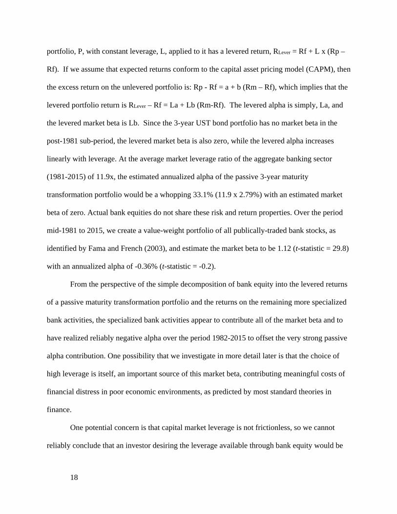
portfolio, P, with constant leverage, L, applied to it has a levered return, RLever = Rf + L x (Rp –

Rf). If we assume that expected returns conform to the capital asset pricing model (CAPM), then

the excess return on the unlevered portfolio is: Rp - Rf = a + b (Rm – Rf), which implies that the

levered portfolio return is RLever – Rf = La + Lb (Rm-Rf). The levered alpha is simply, La, and

the levered market beta is Lb. Since the 3-year UST bond portfolio has no market beta in the

post-1981 sub-period, the levered market beta is also zero, while the levered alpha increases

linearly with leverage. At the average market leverage ratio of the aggregate banking sector

(1981-2015) of 11.9x, the estimated annualized alpha of the passive 3-year maturity

transformation portfolio would be a whopping 33.1% (11.9 x 2.79%) with an estimated market

beta of zero. Actual bank equities do not share these risk and return properties. Over the period

mid-1981 to 2015, we create a value-weight portfolio of all publically-traded bank stocks, as

identified by Fama and French (2003), and estimate the market beta to be 1.12 (t-statistic = 29.8)

with an annualized alpha of -0.36% (t-statistic = -0.2).

From the perspective of the simple decomposition of bank equity into the levered returns

of a passive maturity transformation portfolio and the returns on the remaining more specialized

bank activities, the specialized bank activities appear to contribute all of the market beta and to

have realized reliably negative alpha over the period 1982-2015 to offset the very strong passive

alpha contribution. One possibility that we investigate in more detail later is that the choice of

high leverage is itself, an important source of this market beta, contributing meaningful costs of

financial distress in poor economic environments, as predicted by most standard theories in

finance.

One potential concern is that capital market leverage is not frictionless, so we cannot

reliably conclude that an investor desiring the leverage available through bank equity would be

19

able to achieve her investment goals with investments in more realistically levered passive

maturity transformation strategies. This turns out not to be a meaningful concern for many

investors. Consider an investor who holds the market portfolio of public stocks. Now, restrict

this investor from holding any bank stocks, but instead provide access to the unlevered passive

maturity transformation portfolio. Assuming a one-for-one swap of these exposures (i.e. holding

all other portfolio weights constant) the investor is better off in terms of higher realized mean

return, lower portfolio volatility, higher Sharpe ratio, and higher terminal wealth.7 Overall, these

results are highly inconsistent with the view that bank equity investors are advantaged relative to

capital market alternatives for maturity transformation strategies.

III. Distinctiveness & Relative Advantage of Bank Funding

A bank funding advantage relative to capital markets is a common assumption and

frequent conclusion in the banking literature. It potentially derives from a customer’s willingness

to pay for transaction services via forgone market interest on transactable deposit accounts and

customers may be forced to sacrifice these returns if there is imperfect competition. Government

restrictions on which intermediaries are able to offer transactable accounts and government

deposit insurance make this a unique source of funding for banks (i.e. a distinct funding

technology). Whether this technology is efficient relative to a capital market alternative is a

separate issue that this section investigates. We refer to situations where the bank technology

appears relatively efficient to the closest capital market technology as being advantaged.

7 Allowing the investor to re-optimize the portfolio will improve performance. In general, the differential alphas ensures the improved welfare of the investor for whom the CAPM is a reasonable risk model (Sharpe (1966)).

20

We first explore whether bank customers accept below market investment returns from

claims that do not offer transaction services, but are otherwise money-like (i.e. short-term and

safe). The second issue we explore is whether banks are able produce claims for which

customers are willing to forgo market returns at a sufficiently low cost that they come out ahead

of their alternative funding strategy of issuing debt directly in the capital market.

A. Assessing Customers’ Acceptance of below Market Returns by Bank Funding Type

To provide context on the scope for specialness in bank funding technologies, we first

summarize the various forms of bank debt outstanding for the aggregate banking sector each

quarter from 1998 through 2015. Figure 5 plots the time series of various forms of bank debt

funding – notional values in Panel A and shares of book asset values in Panel B – for the

aggregate banking sector. Our classification of the distinctiveness of the bank technology for

issuing these claims relative to the closest capital market alternative identifies deposits as the

only distinct source of funds. The figure highlights that roughly 40% of bank funding comes

directly from the capital market in the form of repo, debt, and equity, and therefore has no

meaningful distinctiveness. Bank deposits are distinct and account for 60% of bank funding.

A.1Deposits

Our notion of a distinctive technology applies to deposits because these specific claims

are unique to banks. However, banks are not the sole provider of all of the economic functions

these claims support. From the customer perspective, bank deposits offer riskfree investments

with or without transaction services (e.g. term deposits do not provide transaction services).

Short-term riskfree investments are available through portfolios of US Treasury bonds (nearly

21

perfect risk-match since the US Government backs both the bonds it issues and bank deposits)

and relatively safe, although not riskfree, short-term investments are available in the form of

repo, money market mutual funds, and short-term investment grade bonds. This suggests that

transactable deposits have imperfect substitutes and that non-transactable deposits have near

perfect substitutes from the customer perspective.

We are first interested in characterizing the willingness of deposit-holders to forgo

market interest and how this relates to the closeness of available substitutes in terms of economic

function (Merton and Bodie (1993, 1995)). Using the detailed maturity composition of various

deposit account types reported in regulatory filings for each bank, we are able to classify deposits

into transactable and time-deposit accounts and to calculate the average maturity of each of these

categories. The maturity of a deposit account stipulates the period for which depositors cannot

withdraw funds. What we term “transactable accounts” are defined as withdrawable within a

week and includes all checking accounts and savings accounts that allow for multiple

withdrawals within a month. In addition to being demandable, checking and savings accounts

(up to $250K) are also riskfree for investors through FDIC insurance. Time deposits up to $250K

are also FDIC insured.

Figure 6 summarizes the quarterly maturity composition of bank deposits for the

aggregate banking sector over the period 1998 through 2015. The majority of bank deposits,

equivalent to roughly 40% of book value of assets, are transactable deposit accounts. The

remaining “term-deposit accounts” have an average maturity of nearly 15 months over this

sample. The overall value weighted average maturity of deposits, including transactable deposits,

averages just under 5 months.

22

There is considerable empirical support for the notion that customers are willing to pay

for transaction services by accepting less than market interest on transactable deposits (Hannan

and Berger (1991), Neumark and Sharpe (1992), O’Brian (2000), and Krishnamurthy and

Vissing-Jorgensen (2012)). Additionally, the rate banks pay to customers on transactable

accounts is relatively insensitive to changes in the market riskfree interest rate. We confirm these

properties in our sample by comparing the deposit interest rate earned by customers on

transactable accounts, inclusive of the fees charged to customers, to the one-month US Treasury

bill rate. Panel B of Figure 7 displays these quarterly returns. Table 4 reports that the mean

annualized rate earned by investors on transactable deposits between 1997 and 2015 is 0.97%,

while investments in 1-month US Treasury bills earned 2.2% over this period. This significant

difference in returns confirms that bank customers accepted less on their transactable deposit

accounts than their closest capital market alternative investment.

To determine whether these properties extend to time deposits, we do two things. First,

we compare the rates paid on newly issued 6-month certificates of deposit (CDs), secondary

market rates on 6-month CDs, and 6-month US Treasury bills (T-bills). These monthly rates are

displayed in Panel A of Figure 7. The rates on US T-bills and secondary market CDs are

available from 1965 through 2015, while the newly issued CD rates, calculated as the average

rate offered and reported by RateWatch, are available from 1997 through 2015. Clearly, 6-month

CDs are well integrated into capital markets as they are traded in the secondary market. It

appears that, on average, 6-month CDs have reliably higher rates than 6-month US T-bills in the

secondary capital market, with their annualized rates averaging 0.7% higher. The quoted rates on

newly offered 6-month CDs are indistinguishable from 6-month US T-bill yields.

23

This suggests that time deposits may be viewed by customers as having near perfect

capital market substitutes and, as such, they are not willing to forgo market interest for these

non-transactable deposits. To provide further evidence of this possibility, we compare the overall

average rate paid to customers on time deposits to the return that would be earned on a portfolio

of US Treasury bonds with an investment policy of each month purchasing newly issued 18-

month bonds and holding them to maturity. This results in an average portfolio maturity of 9-

months, which is somewhat below that of the aggregate portfolio of time deposits, estimated to

be 15 months. To make this comparison of market returns comparable to the accounting returns

available for banks, we apply the simple book value accounting scheme that we used earlier, to

our capital market portfolio, whereby we maintain security values at par value and use interest

income as it is earned. The results of this analysis are reported in Panel C of Figure 7 and in

Table 4. In each quarter, the rate earned by customers on time deposits looks very similar to the

rate earned by investors in a capital market portfolio of similar maturity with similar reporting.

Additionally, the mean returns on non-transactable deposits and maturity-matched UST bond

portfolios are statistically indistinguishable from each other with small periodic deviations. This

suggests that (1) rates on time deposits are highly sensitive to changes in capital market interest

rates8 and (2) although non-transactable deposits appear by some metrics to be distinct, the scope

for this funding type to provide an advantage for banks is limited because from the customers’

8 Our interpretation of this result contrasts somewhat with the interpretations of Drechsler, Savov, and Schnabl (2017) who find that accounting asset returns net of accounting liability returns are immune to interest rate exposure. We view the apparent insensitivity to interest rates to be primarily a consequence of the accounting treatment and that the economically-relevant interest rate exposures of both assets and liabilities are better estimated from maturity-matched portfolios of US Treasury bond portfolios, with maturities coming from the detailed reported distributions of maturities by asset and liability type at the bank level from regulatory filings.

24

perspectives they have excellent capital market substitutes in terms of economic function

(Merton and Bodie (1993, 1995)). Customers appear to sacrifice market returns only for bank

funding types that offer transaction services (except for equity, as discussed later).

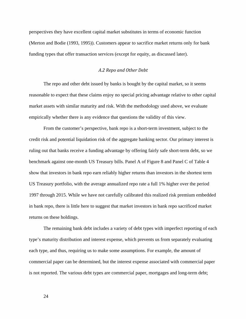
A.2RepoandOtherDebt

The repo and other debt issued by banks is bought by the capital market, so it seems

reasonable to expect that these claims enjoy no special pricing advantage relative to other capital

market assets with similar maturity and risk. With the methodology used above, we evaluate

empirically whether there is any evidence that questions the validity of this view.

From the customer’s perspective, bank repo is a short-term investment, subject to the

credit risk and potential liquidation risk of the aggregate banking sector. Our primary interest is

ruling out that banks receive a funding advantage by offering fairly safe short-term debt, so we

benchmark against one-month US Treasury bills. Panel A of Figure 8 and Panel C of Table 4

show that investors in bank repo earn reliably higher returns than investors in the shortest term

US Treasury portfolio, with the average annualized repo rate a full 1% higher over the period

1997 through 2015. While we have not carefully calibrated this realized risk premium embedded

in bank repo, there is little here to suggest that market investors in bank repo sacrificed market

returns on these holdings.

The remaining bank debt includes a variety of debt types with imperfect reporting of each

type’s maturity distribution and interest expense, which prevents us from separately evaluating

each type, and thus, requiring us to make some assumptions. For example, the amount of

commercial paper can be determined, but the interest expense associated with commercial paper

is not reported. The various debt types are commercial paper, mortgages and long-term debt;

25

subordinated corporate bonds; and trading liabilities. Our approach is to model this overall

category as a portfolio of 1-month US T-bills and a passive strategy that each month purchases a

-maturity A-rated corporate bond. We assume that commercial paper, trading liabilities, and

other borrowed money less than 1-year, representing 70% of this category, are equivalent to 1-

month US T-bills. The remaining 30% has an estimated average maturity of 3-years, which we

mimic by purchasing 6-year A-rated corporate bonds so that the average maturity of this portion

of the portfolio is 3-years. We then adjust these returns to reflect the accounting treatment, as

described earlier. Panel B of Figure 8 and Panel C of Table 4 show that investors in the other

bank debt earned very similar returns to what they would have earned on a portfolio with similar

risk and maturity characteristics.

Overall, it appears reasonable to conclude that the non-deposit debt claims issued by

banks in the capital market are priced consistently with similar capital market alternatives. Thus,

the scope for a potential funding advantage seems to be limited to transactable deposit accounts,

as customers and investors appear to not sacrifice market returns for any other bank liability.

B. Assessing Bank Advantage by Funding Type

The previous subsection shows that the scope for a funding advantage is limited to

transactable deposits, as these are the only claims for which customers sacrifice market returns.

The key question to be addressed in this section is whether banks are able to obtain a practical

funding advantage from their transactable deposits, net of the production costs associated with

supplying these claims and associated transaction services. In addition, we seek to clarify the

scope for banks to obtain an advantage related to the amount of debt that they issue relative to

their assets (i.e. leverage).

26

Banks issue large amounts of relatively safe short-term debt in the form of deposits.

Maintaining these individual deposit accounts requires banks to incur ongoing operating costs,

which we have assumed to be equal to 50% of the total operating costs of banks, with the

remaining 50% being attributed to asset-based activities. The question is whether the sacrificed

market returns on deposits are large enough to justify these deposit-based operating costs, or if

relying entirely on capital market funding would be cheaper.

Define the market returns sacrificed by deposit customers to be , the cost of producing

deposits to be , and the frictional cost of producing nearly riskfree short-term debt in the capital

market to be . The condition for banks to have a funding advantage is - < . We highlight

this condition because the frictional cost of issuing nearly riskfree short-term debt in the capital

market has declined significantly in the later part of the sample with advancements in

technology. For example, portfolio margin9, first introduced around 2000, and becoming widely

available to capital market participants in 2008, relies on real-time portfolio monitoring of

market values, combined with portfolio liquidation rights to offer short-term loans to investors at

rates as low as 25 basis points (bps) over the Federal Funds rate.10 The technology cost required

to perform this activity was likely exorbitant in the early part of our sample, but has declined to

the point where the frictional cost of short-term borrowing in the capital market appear to be

below 25 bps ( 25 bps). Moreover, the amount of leverage available with portfolio margin

9 In 1998, the Board of Governors of the Federal Reserve System amended Regulation T, allowing self-regulated organizations to implement portfolio margin rules (Federal Reserve System (1998)).

10 For example, Interactive Brokers charges 0.25% per year over the Federal Funds rate on margin balances over $3 million, (https://www.interactivebrokers.com/en/index.php?f=interest&p=schedule), accessed September 25, 2017.

27

exceeds the typical deposit-based leverage (i.e. the average ratio of deposits to assets for small

banks is 0.7 and 0.5 for the largest banks). The technology that enables portfolio margin is

essentially continuously stress testing the portfolio to determine the required equity cushion to

keep the loan nearly riskfree and allows for investors in broad-based indices to maintain loans 7x

their marked-to-market equity value (e.g. A=100, L=86, E=14).

This contrasts with the persistently large production costs for banks. Based on the

baseline assumption of s = 0.5, the annual average aggregate production cost of deposits (i.e. the

allocated operating expense divided by deposits) is 2.9%. This is large relative to the average

annual market returns sacrificed by bank deposit holders, which average 1.25% for transactable

deposits and 0% for non-transactable deposits. Thus, bank deposits are highly disadvantaged

relative to capital market funding at the end of our sample.

We summarize the costs of bank deposits relative to capital market debt costs for the

aggregate sample of bank holding companies, as well as by size-based categories of banks. Each

quarter we categorize banks based on their asset value rank, with the largest 5 banks considered

“mega”, the next 50 banks being “large”, the next 100 banks being “medium”, and the remainder

being “small.” For each size category we calculate the value weighted average cost of deposits

across various assumptions for s, the share of non-interest expenses attributed to asset-based

activities. We benchmark these deposit costs against the cost of debt issued by these same banks

over the full sample period from 1997 through 2015 (Panel A), and by subperiods, 1997-2007

(Panel B) and 2008-2015 (Panel C). Additionally, in the latest subperiod, we also benchmark

against the cost of portfolio margin, calculated as the Federal Funds rate plus 25bps. These

results are reported in Table 5.

28

Deposit and debt costs are decreasing in bank size, operating expenses are essentially

identical across size categories, and the share of assets funded with deposits is decreasing in bank

size. This highlights that our calculations with constant s across size categories may not be

directly comparable. For example, one possibility is that a 50% of operating expenses for small

and medium banks should be scaled by the relative deposit-to-asset shares of the mega banks to

smaller banks, such that the corresponding deposit share of operating costs is just over 30% (i.e.

s=0.7). While it is not entirely clear what the proper share of operating expenses is for each size

category, it is clear that deposit costs are larger than debt costs for all but the most extreme

assumptions. As noted above, this is especially true in the later subperiod when compared to

portfolio margin costs (reported in Panel C).

Short-term leverage is routinely supplied in capital markets. A capital market investor or

entrepreneur able to otherwise obtain the asset exposures similar to banks, can obtain financial

leverage by issuing corporate debt, repo, or borrowing via margin loan. This suggests that from

the issuer perspective there are many close substitutes. The empirical results suggests that the

most distinctive type of bank funding – bank deposits – are disadvantaged after costs, while repo

and other bank debt appear to be priced equivalently to capital market alternatives.

IV. The Relative Advantage of Bank Asset Investments

Asset-based banking activities are viewed to have the potential for an advantage relative

to capital markets through specialized credit issuance technology and through low cost sourcing

of potential borrowers through their deposit-taking activities. In addition, they may have

opportunities to provide additional specialized services to their banking customers, which would

present as net income with little required capital. Following the approach developed earlier, we

29

recognize that banking technologies for providing some asset-based economic functions are

distinctive from those used elsewhere in the capital market, but we focus on evaluating whether

these technologies are relatively efficient.

We first measure bank asset returns relative to passive maturity-matched US Treasury

bond portfolios to determine the basic properties of the risk premia banks earn on their assets.

The second issue we explore is whether banks are able to capture more attractive risk premia

than are available elsewhere in the capital market.

A. Risk Premia on Bank Assets

Bank assets are comprised of cash, securities, various types of classified loans (e.g.

business loans, mortgages, consumer loans), and various unclassified investments. On average,

cash and securities account for approximately 30% of book assets, classified loans account for

approximately 50% of book assets, with the remaining 20% of book assets being unclassified

investments. Figure 10 displays the quarterly asset composition of these categories (Panel A) and

as shares of total assets (Panel B). In addition, there is fairly rich data at the bank level describing

the maturity distribution of assets, including information within the security and loan categories.

Banks are required to report the remaining maturity on their assets for fixed interest rate

contracts by reporting the amount of time remaining from the date of the filing (FR-Y-9C or

equivalent) until the final contractual maturity of the instruments. For floating rate contracts,

banks report the amount of time between the date of the filing and the next repricing date or the

contractual maturity, whichever is earlier. Therefore, the reported maturities measure the period

over which interest rates are contractually fixed, as opposed to the notional maturity of the asset.

Figure 10 also displays the reported quarterly maturity distributions for securities and loans, and

30

our estimates for total assets. To estimate the maturity distribution for assets, we assume (1)

specific maturities for the maturity categories reported for securities and loans and (2) specific

maturities for cash and other unclassified assets. The following table shows our maturity

assumptions for the reported categories:

Reported Maturity Category <3mo 3mo-1yr 1yr-3yr 3yr-5yr 5yr-15yr >15yr Assumed Maturity in Months 1 7 24 48 120 180

We assume that cash and Federal Funds sold have maturity of one-month (maturity category 1)

and that the unclassified other assets have a maturity of seven months (maturity category 2). We

view these assignments to be conservative, as the unclassified investments include unclassified

loans and other relatively long-lived investments. This allows us to estimate the maturity

distribution for total assets. For the benchmark portfolio, we model this maturity distribution as a

weighted average of shortest-term maturity and the average maturity (long-term average

maturity) across the remaining categories, so that the passive portfolio invests to achieve a

similar maturity distribution by investing in one-month US T–bills and each month purchasing h-

maturity bonds, where h is 2 times the long-term average maturity, and holding these until

maturity to produce an average maturity similar to the long-term average maturity of bank assets.

The bottom-left panel of Figure 10 displays the average asset maturity and the long-term average

maturity. There is also considerable information about the income from each asset category,

which allows us to construct the returns to various asset categories. We subtract the accounting

returns from the associated maturity-matched passive portfolio strategies of US Treasury bonds

to measure realized risk premia.

31

We calculate the unlevered return on assets by removing the effects of financing to

isolate the net income earned on asset-based activities. Specifically, we calculate the return on

book assets in quarter t as:

, (1)

where NI is net income, DepositIncome is service charges on deposits, OpEx is non-interest

expenses, s is the share of non-interest expenses allocated to asset-based activities, and is the

tax rate assumed to be 0.3.11 Aggregate bank assets have an average maturity of 2.84 years,

comprised of 38.7% short-term assets with an average maturity of one-month and 61.3% longer-

term assets with an average maturity of 4.52 years. With the baseline assumption that s = 0.5, the

annualized return on aggregate bank assets averages 3.37% over the period 1997 to 2015. A

passive portfolio designed to match this maturity distribution with buy-and-hold investments in

US Treasury bonds earns 3.94% on average, producing a reliably negative realized risk premium

for bank assets of -.47% per year (t-statistic = -3.35). Figure 11 displays the quarterly time series

of these annualized returns, showing that the accounting returns on the simple benchmark

portfolio track the asset returns well and that the gap in returns is not driven by the 2008

financial crisis, as the UST portfolio has higher returns in the pre-crisis period. This suggests that

bank assets have not earned positive risk premia for the credit and illiquidity risks in their asset

portfolios.

11 We calculate the tax rate as, 1 . The time series average aggregate tax rate is 29.9%.

32

Table 6 summarizes these calculations for various assumptions about the share of

operating expenses allocated to asset-based activities and across various bank size categories, as

described earlier. It is useful to note that smaller banks tend to have longer reported maturities

and larger allocations to loans than larger banks. The differences in maturity are captured in the

maturity-based benchmark, but the potential credit risk differences are not. With the assumption

that only 30% of operating expenses are due to asset-based activities, the aggregate bank asset

risk premium averages zero and is reliably negative for the medium and small banks. At all other

considered asset-based activity shares of operating expenses, aggregate asset risk premium are

reliably negative.

B. Bank Investment Returns by Asset Category

In light of the remarkable finding that the realized risk premium for bank assets has been

zero with the most generous assumptions, and likely to have been reliably negative over the

period 1997-2015, we investigate the realized risk premia by asset category. We view this

exercise as providing some robustness checks on our basic methodology as we can evaluate

whether the simple benchmark returns, adjusted for accounting rules, track returns well across

asset types and bank size categories.

We first calculate bank returns by asset type and determine the benchmark strategy based

on the maturity distribution of each asset type. The return on cash and Federal Funds sold is

calculated simply as the quarterly interest income on these two categories divided by their

beginning of period balances. The return on securities and on loans are calculated as follows:

, (2)

33

, (3)

where CL denotes classified loans. We assume that there are no overhead charges associated

with managing the securities portfolio. Since bank loans are issued with a distinctive specialized

technology, the management of these investments is likely to generate some of the operating

expenses. We assume that their share of operating expenses is proportional to their asset share,

. This leaves the return on other assets to be defined as the residual unlevered income

divided by beginning of period other assets. The results of these calculations, at the baseline

assumption of s = 0.5, are summarized in Figure 12, which shows the relative investment

performance across asset types by bank size category.

Figure 12 shows that the simple maturity-matched benchmark portfolios track the time

trends in returns well except for the other assets. As expected, the security returns look very

similar to their UST benchmarks and have similar means. The loan returns also look quite similar

to the UST benchmarks and have similar returns, which indicates that they earn no risk premium

for the credit and illiquidity risk they bear. This is driven by the loan returns of the mega banks,

which are -0.5% per year lower than their benchmark with s = 0.5. The bank loan risk premia for

all other size categories are reliably positive. The most striking returns are those associated with

the other assets, which capture the profits from many of the most distinctive asset-based bank

activities. These returns are reliably negative for all size categories and cost assumptions. These

results push against the view that the synergies from combining deposit-taking and credit

issuance are positive, as the economic returns from these synergies are a component of these

returns.

34

C. Credit Risk Premia in the Capital Market

One natural concern is that the realized risk premia on bank assets that we have measured

over the period 1997 through 2015 are biased down because of the 2008 financial crisis. During

this period, banks realized credit losses that were large relative to what was expected, which

could lead to realized returns that are considerably lower than what was expected ex ante. We

investigate this possibility by examining the excess returns to passive credit portfolios available

in the capital market. Specifically, we examine the returns to several Vanguard index funds that

passively invest in either investment grade or high yield bonds and compare these funds to their

maturity-matched UST index also managed by Vanguard. There are three different UST indices

with maturities described as short-term, intermediate-term, and long-term. Since bank assets are

relatively short-term, we do not consider the long-term portfolios.12 Vanguard has a short-term

investment grade portfolio and an intermediate-term high yield portfolio. The maturity-matched

annualized excess returns are 0.52% and 0.53% for the investment grade and high yield

portfolios, respectively. This is consistent with the notion that short- and intermediate-term credit

risk premia were positive elsewhere in the capital market over this period.

12 The Vanguard short-term US Treasury index has an annualized mean return of 3.7%, while the Vanguard intermediate-term US Treasury index has an annualized mean return of 5.5%. Our maturity-matched UST portfolio designed to match aggregate bank asset maturity has an annualized mean return of 4%, suggesting that the short-term maturity index is a better maturity-match than the intermediate-term index.

35

V. Consequences and Implications for Bank Equity

The empirical evidence suggests that bank assets underperform US Treasury portfolios

and that bank deposits are a relatively inefficient source of funding for banks, which together

translate into bank equity underperforming its passive capital market opportunity cost. As

demonstrated earlier, from the perspective of common equity risk models (e.g. CAPM) this

underperformance can be masked by the strong performance of the passive components of the

bank business model. Recall that an unlevered maturity-matched passive portfolio of US

Treasury bonds had a market beta of zero and an annualized alpha of 2% from 1981 through

2015, while bank equity had a market beta over 1 and an annualized alpha of zero over this

period.

In the aggregate, bank assets are relatively safe and the well-classified assets are mostly

free of market beta.13 This suggests that the source of the market beta may be the unclassified

assets and banks’ leverage policy itself, both of which can be viewed as highly distinctive

relative to other capital market activities. To illustrate one possible way to reconcile the

relatively high market betas of bank equities with the extremely low market betas of the

classified bank assets is to model the unclassified assets as high yield bonds. Specifically, we

consider a pseudo bank asset portfolio as being a combination of 30% short-term US Treasury

bonds, 50% short-term investment grade bonds, and 20% intermediate-term high yield bonds, all

proxied with Vanguard funds. This unlevered portfolio has a market beta of 0.066 (t-statistic =

13 A portfolio that invests 50% in short-term investment grade bonds and 50% in short-term US Treasury bonds has a market beta of zero over the period 1981 through 2015.

36

6.9) and an annualized alpha of 1.8% (t-statistic = 3.3) over the period 1997 through 2015. In

2008, this unlevered pseudo-bank portfolio has a drawdown of nearly -9%, as illustrated in Panel

A of Figure 13.

Consider how leverage affects the risk of the equity on this portfolio. In the period shortly

before the financial crisis, the aggregate bank leverage based on book values was around 15x

(see Figure 4). This drawdown levered 15x is expected to essentially exhaust the equity. To

account for the fact that the drawdown is not experienced immediately, we calculate the levered

equity returns to the pseudo-bank assuming both that the portfolio is levered 15x and 5x,

maintaining these target leverages through monthly rebalancing. The cumulative equity returns

are displayed in Panel B of Figure 13, along with the cumulative returns to the aggregate banking

sector equity portfolio. We approximate the portfolio margin requirement as 15% of the

portfolio’s previous maximum value and plot this value along with the cumulative equity levels.

In the depths of the financial crisis, the relatively small losses of the pseudo-bank asset portfolio

are translated into losses that trigger a sustained margin call for the pseudo-bank equity that is

levered 15x.

A capital market portfolio approaching a margin call can (1) hope prices recover and do

nothing; (2) sell assets; and (3) raise equity capital. Option (1) is clearly risky, but will

sometimes work. Options (2) and (3) can be costly to equity investors, as asset sales of illiquid

specialized assets may occur at fire sale prices, and the cost of equity capital may be especially

high during periods of poor economic conditions. From this capital market perspective, it is not

surprising to find that banks are forced to issue large amounts of equity at these times. Black,

Floros, and Sengupta (2016) find that banks issue approximately $50 billion worth of equity in

the last quarter of 2008. This is approximately 5% of the total market value of publically traded

37

bank equity in a single quarter, at a time when bank equities are trading at less than one-half their

previous high values. This is especially perverse from the perspective of one who is inclined to

believe that high leverage is a useful way for banks to avoid the frictional costs of issuing equity

(e.g. Baker and Wurgler (2015)). It is also useful to note that the pseudo-bank levered 5x does

not come close to a margin call and has mean equity returns that are nearly identical to those for

actual banks with one-third of the market beta, over the period 1997 to 2015. This leads to a

marginally reliable difference in annualized alphas of -11.5% (t-statistic = 1.88).

VI. Conclusion

This paper argues that despite a widespread belief in bank specialness, the evidence on

the efficiency of distinctive bank technologies relative to those used elsewhere in the capital

market is scarce. The evidence presented here suggests that bank activities appear to be

inefficient relative to their closest capital market substitutes. Moreover, there is some tendency

for the most distinctive components of the bank business model to be the most inefficient, which

is in direct conflict with the notion of bank specialness.

38

39

References

Admati, Anat, Peter DeMarzo, Martin Hellwig, and Paul Pfleiderer, 2013, “Fallacies, Irrelevant Facts, and Myths in the Discussion of Capital Regulation: Why Bank Equity is Not Socially Expensive” Stanford working paper.

Baker, Malcolm and Jeffrey Wurgler, 2015, “Do Strict Capital Requirements Raise the Cost of Capital? Bank Regulation, Capital Structure and the Low Risk Anomaly” American Economic Review: Papers and Proceedings 105, no. 5, 315-320.

Begenau, Juliane, Monika Piazzesi, Martin Schneider, 2015 “Banks’ Risk Exposure”, working paper

Berger, Allen, 1995, “The Relationship between Capital and Earnings in Banking” Journal of Money, Credit, and Banking 27, no. 2, 432-456.

Berger, A.N. and Bouwman, C.H., 2009. Bank liquidity creation. Review of Financial Studies, 22(9), pp.3779-3837.

Berger, A.N. and Bouwman, C.H., 2013, “How does capital affect bank performance during financial crises?” Journal of Financial Economics 109, no. 1, 146-176.

Black, Lamont, Ioannis Floros, and Rajdeep Sengupta, 2016, “Raising Capital When the Going Gets Tough: U.S. Bank Equity Issuance from 2001 to 2014”, Federal Reserve Bank of Kansas City Research Working Paper.

Cochrane, John, 2014, Across the Great Divide: New Perspectives on the Financial Crisis, Martin Neil Baily, John B. Taylor, eds., Hoover Press.

Damodaran, Aswath, 2006. Damodaran on Valuation: Security Analysis for Investment and Corporate Finance, 2nd Edition, John Wiley & Sons.

Diamond, D.W., 1984. Financial intermediation and delegated monitoring. The Review of Economic Studies, 51(3), pp.393-414.

Diamond, D.W. and Rajan, R.G., 2000. A theory of bank capital. The Journal of Finance, 55(6), pp.2431-2465.

Diamond, D.W. and R.G. Rajan., 2001, “Liquidity risk, liquidity creation and financial fragility: a theory of banking” Journal of Political Economy, 109, pp. 287–327

Drechsler, Itamar, Alexi Savov, and Phillip Schnabl, 2017, “Banking on Deposits: Maturity Transformation without Interest Rate Risk,” New York University working paper.

40

Fahlenbrach, R., Prilmeier, R. and Stulz, R.M., 2016. Why Does Fast Loan Growth Predict Poor Performance for Banks? (No. w22089). National Bureau of Economic Research.

Fama, Eugene F, 2006, “The Behavior of Interest Rates,” The Review of Financial Studies 19, no. 2, 359-379.

Fama, Eugene F, Kenneth R. French, 1997, “Industry Costs of Equity,” Journal of Financial Economics 47, 153-193.

Federal Reserve System, 1998, “Securities Credit Transactions; Borrowing By Broker and Dealers,” Regulations G, T, U and X; Dockets Nos. R-0905, R-0923 and R-0944, 63 FR 2806 (January 16, 1998).

Flannery, Mark J., and Sorin M. Sorescu, 1996, "Evidence of bank market discipline in subordinated debenture yields: 1983–1991" The Journal of Finance 51, no. 4, 1347-1377.

Gatev, Evan and Philip Strahan, “Banks’ Advantage in Hedging Liquidity Risk: Theory and Evidence from the Commercial Paper Market,” Journal of Finance 61, 867-892.

Gorton, G., and G. Pennacchi, 1990, “Financial intermediaries and liquidity creation” Journal of Finance, 45, pp. 49–71

Gropp, Reint, and Florian Heider, 2010, "The determinants of bank capital structure" Review of Finance 14, no. 4, 587-622

Hannan, Timothy H., and Allen N. Berger. "The Rigidity of Prices: Evidence from the Banking Industry." The American Economic Review 81, no. 4 (1991): 938-45.

Kashyap, Anil K., Raghuram Rajan, and Jeremy C. Stein, 2002, “Bank as Liquidity Providers: An Explanation for the Coexistence of Lending and Deposit Taking” TheJournalofFinance57, no. 1, 33–73.

Krishnamurthy, Arvind, and Annette Vissing-Jorgensen. "The aggregate demand for treasury debt." Journal of Political Economy 120, no. 2 (2012): 233-267.

Leland, Hayne E., and David H. Pyle. "Informational Asymmetries, Financial Structure, and Financial Intermediation." The Journal of Finance 32, no. 2 (1977): 371-87.

Linter, John, 1965, “The valuation of risk assets and the selection of risky investments in stock portfolios and capital budgets” ReviewofEconomicsofStatistics47, 13–37.

Mehran, H. and Thakor, A., 2011. Bank capital and value in the cross-section. Review of Financial Studies, 24(4), pp.1019-1067.

Merton, R.C., 1977. An analytic derivation of the cost of deposit insurance and loan guarantees an application of modern option pricing theory. Journal of Banking & Finance, 1(1), pp.3-11.

41

Merton, R.C., 1987. A simple model of capital market equilibrium with incomplete information. The journal of finance, 42(3), pp.483-510.

Merton, R.C. and Bodie, Z., 1993, Deposit insurance reform: a functional approach. In Carnegie-Rochester Conference Series on Public Policy (Vol. 38, pp. 1-34). North-Holland.

Merton, R.C. and Bodie, Z., 1995. A conceptual framework for analyzing the financial system. The global financial system: A functional perspective, pp.3-31.

Miller, Merton H, 1995, "Do the M & M propositions apply to banks?" Journal of Banking & Finance 19, no. 3, 483-489.

Modigliani, Franco and Merton Miller, 1958, “The Cost of Capital, Corporation Finance and the Theory of Investment” American Economic Review 53, no. 3, 433-443.

Neumark, David, and Steven A. Sharpe. "Market Structure and the Nature of Price Rigidity: Evidence from the Market for Consumer Deposits." The Quarterly Journal of Economics 107, no. 2 (1992): 657-80.

O’Brian, James, 2000, “Estimating the Value and Interest Rate Risk of Interest-Bearing Transaction Deposits,” Federal Reserve working paper.

Sharpe, William F., 1964, “Capital asset prices: A theory of market equilibrium under conditions of risk” JournalofFinance19, 425–442.

Shleifer, Andrei, Vishny, Robert, 1992. Liquidation values and debt capacity: a market equilibrium approach. Journal of Finance 47, 1343–1366.

Shleifer, Andrei, Vishny, Robert, 1997. The limits to arbitrage. Journal of Finance 52, 35–55.

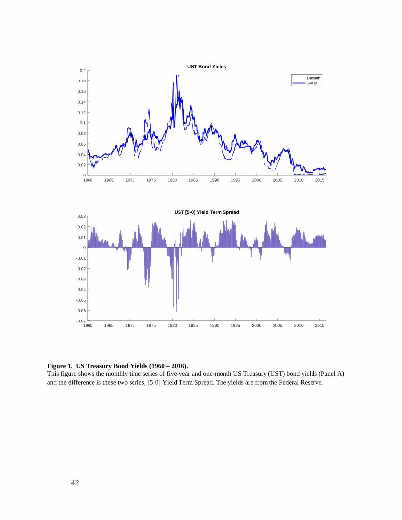
42

Figure 1. US Treasury Bond Yields (1960 – 2016). This figure shows the monthly time series of five-year and one-month US Treasury (UST) bond yields (Panel A) and the difference is these two series, [5-0] Yield Term Spread. The yields are from the Federal Reserve.

1960 1965 1970 1975 1980 1985 1990 1995 2000 2005 2010 20150

0.02

0.04

0.06

0.08

0.1

0.12

0.14

0.16

0.18

0.2UST Bond Yields

1-month5-year

1960 1965 1970 1975 1980 1985 1990 1995 2000 2005 2010 2015-0.07

-0.06

-0.05

-0.04

-0.03

-0.02

-0.01

0

0.01

0.02

0.03UST [5-0] Yield Term Spread

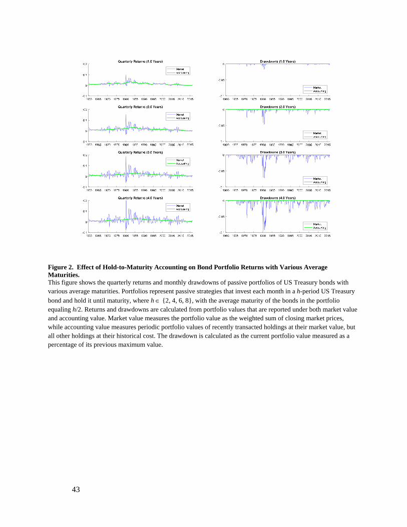
43

Figure 2. Effect of Hold-to-Maturity Accounting on Bond Portfolio Returns with Various Average Maturities. This figure shows the quarterly returns and monthly drawdowns of passive portfolios of US Treasury bonds with various average maturities. Portfolios represent passive strategies that invest each month in a h-period US Treasury

bond and hold it until maturity, where h {2, 4, 6, 8}, with the average maturity of the bonds in the portfolio equaling h/2. Returns and drawdowns are calculated from portfolio values that are reported under both market value and accounting value. Market value measures the portfolio value as the weighted sum of closing market prices, while accounting value measures periodic portfolio values of recently transacted holdings at their market value, but all other holdings at their historical cost. The drawdown is calculated as the current portfolio value measured as a percentage of its previous maximum value.

44

Figure 3. Annual Returns on Aggregate Bank Assets and Costs of Various Bank Debt.

This figure shows the annual asset returns and debt costs for the aggregate commercial banking sector. Panel A displays the return on assets, calculated as net income plus interest expense minus service charges on deposit accounts plus (1-s) times non-interest expense, all divided by the previous period assets, where s represents the share

of non-interest expense allocated to asset-based activities. We consider s {0.3, 0.5, 0.7} and focus on s = 0.5 as our baseline. Panel A also plots the market and accounting returns on a passive portfolio that invest each month in a six-year US Treasury bond and holds it until maturity with a three-year average maturity of the bonds in the portfolio. In Panel B, the annual cost of deposits is calculated as deposit interest minus service charges on deposit

accounts + (1 – s) times non-interest expense, all divided by the previous period deposits. We consider s {0.5, 1.0}. We calculate the cost of non-deposit debt as interest expense minus deposit interest, all divided by the previous period debt. We measure debt from the balance sheet identity, assets minus total equity minus deposits.

1960 1965 1970 1975 1980 1985 1990 1995 2000 2005 2010 2015-0.05

0

0.05

0.1

0.15

0.2

0.25

0.3Annual Returns on Aggregate Bank Asset

Banks 30% expense allocation to assetsBanks 50% expense allocation to assetsBanks 70% expense allocation to assetsUST MarketUST Accounting

1960 1965 1970 1975 1980 1985 1990 1995 2000 2005 2010 2015-0.02

0

0.02

0.04

0.06

0.08

0.1

0.12Bank Deposit and Debt Costs

Bank Deposits 100% expense allocation to assetsBank Deposits 50% expense allocation to assetsBanks Non-Deposit Debt

45

Figure 4. Commercial Banking Sector Leverage. Panel A displays time series plots of aggregate leverage. Leverage is the ratio of aggregate assets to aggregate equity, calculated for the sample of publically-traded firms covered in the CRSP-Compustat Merged Database. Banks are identified based on the criterion in Fama and French (1997), leaving all other firms as non-banks. Market (book) values of assets and equity are used to calculate market (book) leverage. Panel B displays the ratio of aggregate equity to aggregate assets resulting from a stress test, assuming that a shock to asset values were to occur. The shock is -7.64%, estimated as the worst realized drawdown for the three-year UST bond portfolio over the period 1960-2015, applied to the aggregate banking sector assets. Post-shock equity values are calculated as, E* = A (1+shock) – D.

1960 1965 1970 1975 1980 1985 1990 1995 2000 2005 2010 20150

5

10

15

20

25

30

35Bank Leverage (A/E)

Banks (Market)Banks (Book)Non-Banks (Market)Non-Banks (Book)

1960 1965 1970 1975 1980 1985 1990 1995 2000 2005 2010 2015-0.1

-0.05

0

0.05

0.1

0.15

0.2Post-Shock Equity-to-Assets

Banks (Market)Banks (Book)

46

Figure 5. Aggregate Funding Composition for Bank Holding Companies (1997-2015). Panel A displays quarterly composition of aggregate bank capital structure. Bank funding types are deposits, repo, and other bank debt. Panel B displays the quarterly composition of aggregate bank capital structure scaled by aggregate assets.

1996 1998 2000 2002 2004 2006 2008 2010 2012 2014 20160

2000

4000

6000

8000

10000

12000

14000

$ B

illio

nsBank Debt

DepositsRepoOther Bank Debt

1996 1998 2000 2002 2004 2006 2008 2010 2012 2014 20160

10

20

30

40

50

60

70

80

90

100

perc

ent

Bank Debt Asset Share

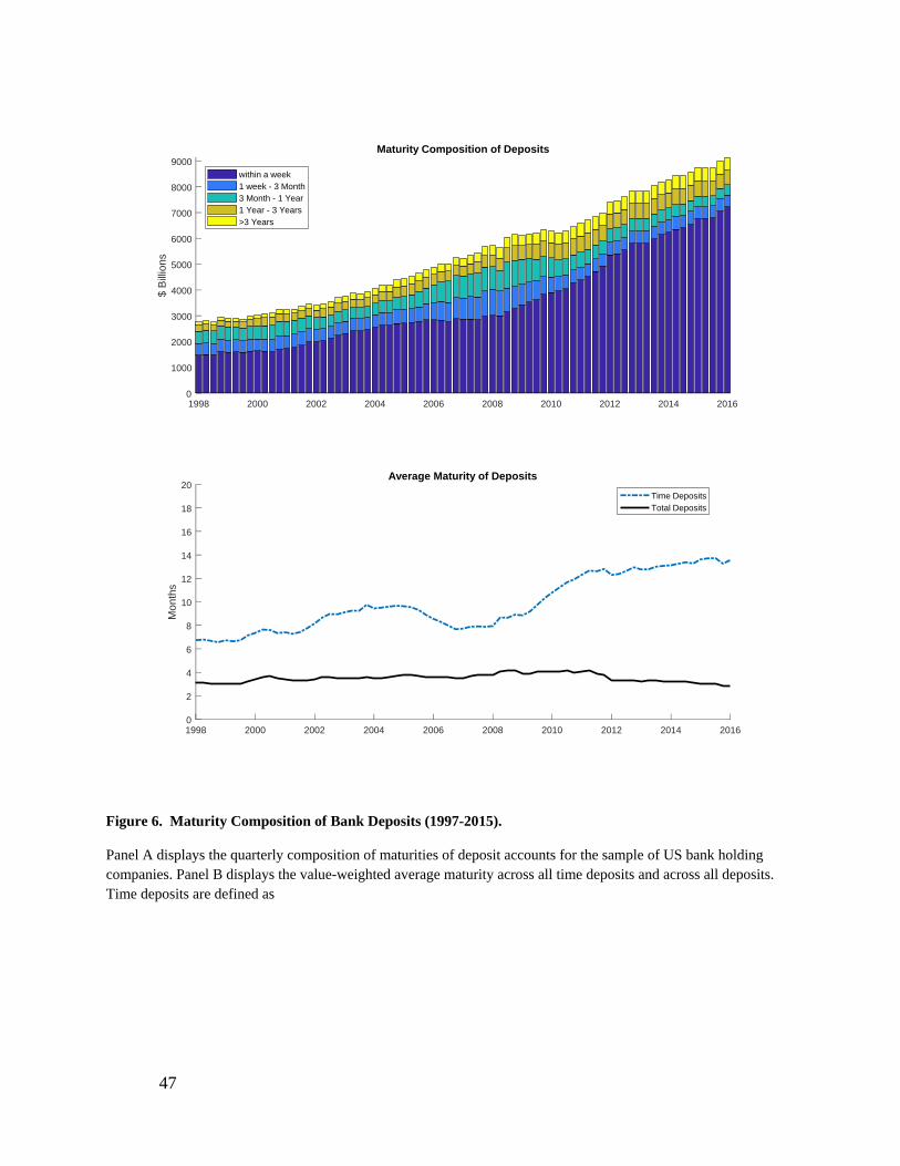
47

Figure 6. Maturity Composition of Bank Deposits (1997-2015). Panel A displays the quarterly composition of maturities of deposit accounts for the sample of US bank holding companies. Panel B displays the value-weighted average maturity across all time deposits and across all deposits. Time deposits are defined as

1998 2000 2002 2004 2006 2008 2010 2012 2014 20160

1000

2000

3000

4000

5000

6000

7000

8000

9000$

Bill

ions

Maturity Composition of Deposits

within a week1 week - 3 Month3 Month - 1 Year1 Year - 3 Years>3 Years

1998 2000 2002 2004 2006 2008 2010 2012 2014 20160

2

4

6

8

10

12

14

16

18

20

Mon

ths

Average Maturity of Deposits

Time DepositsTotal Deposits

48

Figure 7. Rates on Bank Deposits Compared to Customers’ Capital Market Alternatives. Panel A displays monthly annualized yields on 6-month certificates of deposit (CD) and 6-month US Treasury (UST) bonds trading in the capital market. The solid blue line corresponds to secondary market CD yields, the dashed (dash-dot) red line represents offers (quotes) for newly issued CDs, and the black dashed line shows the UST yield. The bottom panels compare annualized yields on transactable deposits (Panel B) and time deposits (Panel C) to the yields on maturity-matched UST portfolios. Transactable deposits are compared to one-month UST yields and time deposits are compared to the accounting returns on a passive portfolio that invest each month in 18-month UST bonds and holds it until maturity with a 9-month average maturity of the bonds in the portfolio.

1970 1975 1980 1985 1990 1995 2000 2005 2010 2015

2

4

6

8

10

12

14

16%

p.a

.

6-Month CD Rates

6-mo CD Secondary Market6-mo UST Secondary Market6-mo CD Month RateWatch Quote

2000 2005 2010 20150

1

2

3

4

5

6

7

8

% p

.a.

Within a Week Bank Deposits

Transactable Deposits1-mo US T-bill

2000 2005 2010 20150

1

2

3

4

5

6

7

8

% p

.a.

Beyond a Week Bank Deposits

Time DepositsAccounting Return UST (9 Months)

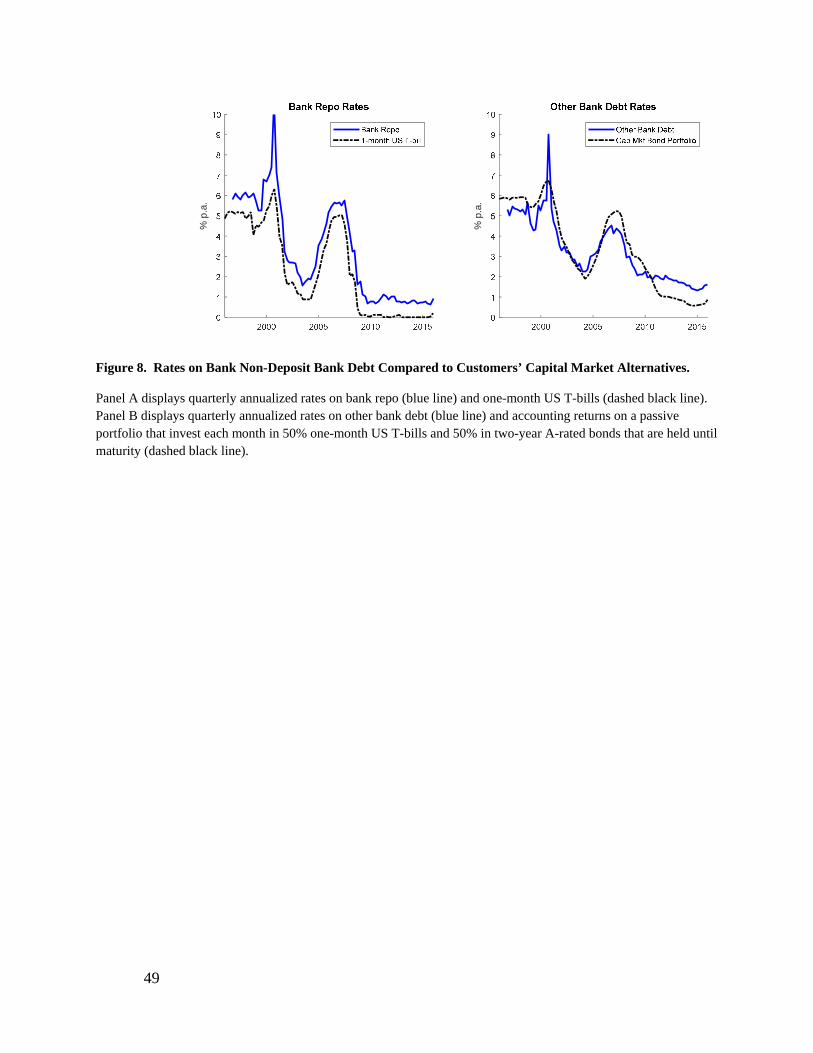
49

Figure 8. Rates on Bank Non-Deposit Bank Debt Compared to Customers’ Capital Market Alternatives. Panel A displays quarterly annualized rates on bank repo (blue line) and one-month US T-bills (dashed black line). Panel B displays quarterly annualized rates on other bank debt (blue line) and accounting returns on a passive portfolio that invest each month in 50% one-month US T-bills and 50% in two-year A-rated bonds that are held until maturity (dashed black line).

% p

.a.

% p

.a.

50

Figure 9. Short-term Funding Costs. The annualized costs of deposits (blue line) are calculated each quarter as deposit interest minus service charges on deposit accounts + (1 – s) times non-interest expense, all divided by the previous period deposits, where s=0.5, is the share of non-interest expense that we allocate to asset-based activities. We calculate the cost of bank debt as interest expense minus deposit interest, all divided by the previous period debt. We measure debt from the balance sheet identity, assets minus total equity minus deposits. The portfolio margin rate is calculated as the annualized Federal Funds rate plus 0.25% (dotted black line), which is displayed over the entire sample period, but only becomes a feasible funding source beginning in 2008.

% p

.a.

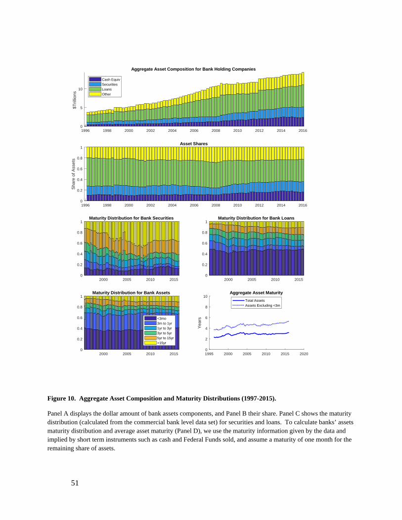
51

Figure 10. Aggregate Asset Composition and Maturity Distributions (1997-2015). Panel A displays the dollar amount of bank assets components, and Panel B their share. Panel C shows the maturity distribution (calculated from the commercial bank level data set) for securities and loans. To calculate banks’ assets maturity distribution and average asset maturity (Panel D), we use the maturity information given by the data and implied by short term instruments such as cash and Federal Funds sold, and assume a maturity of one month for the remaining share of assets.

1996 1998 2000 2002 2004 2006 2008 2010 2012 2014 20160

5

10

$Tril

lions

Aggregate Asset Composition for Bank Holding Companies

Cash EquivSecuritiesLoansOther

1996 1998 2000 2002 2004 2006 2008 2010 2012 2014 20160

0.2

0.4

0.6

0.8

1

Sha

re o

f Ass

ets

Asset Shares

2000 2005 2010 20150

0.2

0.4

0.6

0.8

1Maturity Distribution for Bank Securities

2000 2005 2010 20150

0.2

0.4

0.6

0.8

1Maturity Distribution for Bank Loans

2000 2005 2010 20150

0.2

0.4

0.6

0.8

1Maturity Distribution for Bank Assets

<3mo3m to 1yr1yr to 3yr3yr to 5yr5yr to 15yr>15yr

1995 2000 2005 2010 2015 20200

2

4

6

8

10

Yea

rs

Aggregate Asset Maturity

Total AssetsAssets Excluding <3m

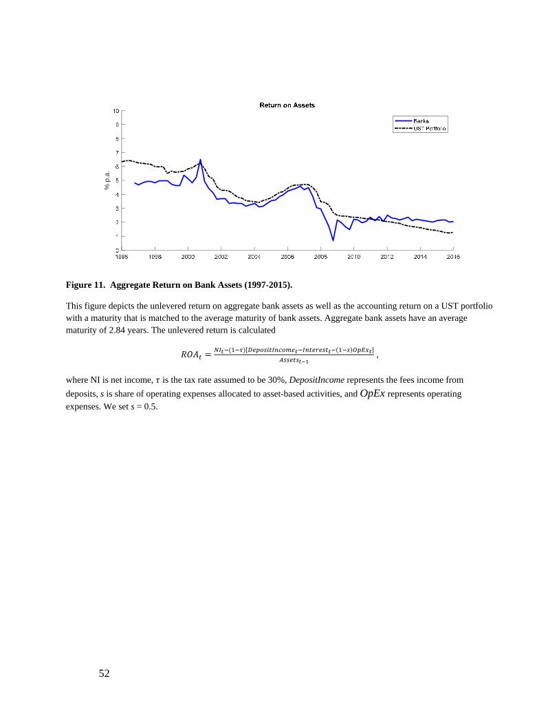
52

Figure 11. Aggregate Return on Bank Assets (1997-2015). This figure depicts the unlevered return on aggregate bank assets as well as the accounting return on a UST portfolio with a maturity that is matched to the average maturity of bank assets. Aggregate bank assets have an average maturity of 2.84 years. The unlevered return is calculated

,

where NI is net income, is the tax rate assumed to be 30%, DepositIncome represents the fees income from

deposits, s is share of operating expenses allocated to asset-based activities, and OpEx represents operating expenses. We set s = 0.5.

% p

.a.

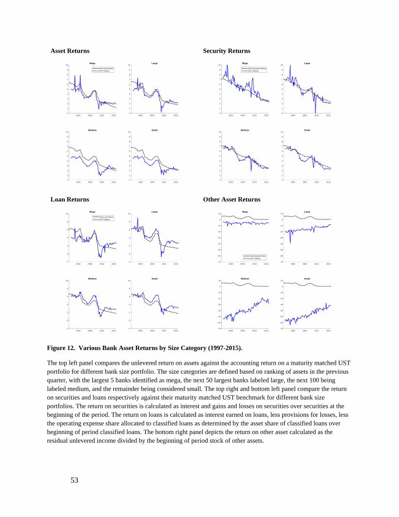
53

Asset Returns Security Returns

Loan Returns Other Asset Returns

Figure 12. Various Bank Asset Returns by Size Category (1997-2015). The top left panel compares the unlevered return on assets against the accounting return on a maturity matched UST portfolio for different bank size portfolio. The size categories are defined based on ranking of assets in the previous quarter, with the largest 5 banks identified as mega, the next 50 largest banks labeled large, the next 100 being labeled medium, and the remainder being considered small. The top right and bottom left panel compare the return on securities and loans respectively against their maturity matched UST benchmark for different bank size portfolios. The return on securities is calculated as interest and gains and losses on securities over securities at the beginning of the period. The return on loans is calculated as interest earned on loans, less provisions for losses, less the operating expense share allocated to classified loans as determined by the asset share of classified loans over beginning of period classified loans. The bottom right panel depicts the return on other asset calculated as the residual unlevered income divided by the beginning of period stock of other assets.

2000 2005 2010 20150

1

2

3

4

5

6

7

8

9

10Mega

Bank Asset ReturnUST Portfolio

2000 2005 2010 20150

1

2

3

4

5

6

7

8

9

10Large

2000 2005 2010 20150

1

2

3

4

5

6

7

8

9

10Medium

2000 2005 2010 20150

1

2

3

4

5

6

7

8

9

10Small

2000 2005 2010 20150

1

2

3

4

5

6

7

8

9

10Mega

Bank Securities ReturnUST Portfolio

2000 2005 2010 20150

1

2

3

4

5

6

7

8

9

10Large

2000 2005 2010 20150

1

2

3

4

5

6

7

8

9

10Medium

2000 2005 2010 20150

1

2

3

4

5

6

7

8

9

10Small

2000 2005 2010 2015-2

0

2

4

6

8

10Mega

Bank Loan Return

UST Portfolio

2000 2005 2010 2015-2

0

2

4

6

8

10Large

2000 2005 2010 2015-2

0

2

4

6

8

10Medium

2000 2005 2010 2015-2

0

2

4

6

8

10Small

2000 2005 2010 2015-70

-60

-50

-40

-30

-20

-10

0

10Mega

Bank Special Return

UST Portfolio

2000 2005 2010 2015-70

-60

-50

-40

-30

-20

-10

0

10Large

2000 2005 2010 2015-70

-60

-50

-40

-30

-20

-10

0

10Medium

2000 2005 2010 2015-70

-60

-50

-40

-30

-20

-10

0

10Small

54

Figure 13. Effect of Leverage on Bank Equity. The top panel presents the drawdowns on the assets of a pseudo bank with 30% short-term UST, 50% short-term investment grade bonds, and 20% intermediate-term high yield bonds available from Vanguard. The bottom panel depicts the cumulative bank equity return (available from CRSP) against that of the pseudo-bank levered 5x (available in capital markets) as well as 15x (aggregate banking sector leverage). The bottom panel also presents the portfolio margin requirement of the pseudo bank at 15x leverage calculated as 15% of the portfolio’s previous maximum value.

2005 2007 2009 2011 2013 2015-0.09

-0.08

-0.07

-0.06

-0.05

-0.04

-0.03

-0.02

-0.01

0Drawdowns on Pseudo-Bank Asset Portfolio

2005 2007 2009 2011 2013 20150

0.5

1

1.5

2

2.5

3

3.5

4

4.5

5Compounded Returns on Bank Equity

Bank EquityPseudo Bank Equity (Leverage = 5x)Pseudo Bank Equity (Leverage = 15x)Portfolio Margin Requirement (Leverage = 15x)

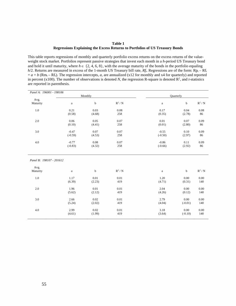
55

Table 1

Regressions Explaining the Excess Returns to Portfolios of US Treasury Bonds This table reports regressions of monthly and quarterly portfolio excess returns on the excess returns of the value-weight stock market. Portfolios represent passive strategies that invest each month in a h-period US Treasury bond and hold it until maturity, where h {2, 4, 6, 8}, with the average maturity of the bonds in the portfolio equaling h/2. Returns are measured in excess of the 1-month US Treasury bill rate, Rft. Regressions are of the form: Rpt – Rft = a + b (Rmt – Rft). The regression intercepts, a, are annualized (x12 for monthly and x4 for quarterly) and reported in percent (x100). The number of observations is denoted N, the regression R-square is denoted R2, and t-statistics are reported in parenthesis.

Panel A: 196001 - 198106 Monthly Quarterly

Avg. Maturity a b R2 / N a b R2 / N

1.0 0.21 0.03 0.08 0.17 0.04 0.08

(0.58) (4.68) 258 (0.35) (2.78) 86

2.0 0.06 0.05 0.07 0.01 0.07 0.09 (0.10) (4.41) 258 (0.01) (2.80) 86

3.0 -0.47 0.07 0.07 -0.55 0.10 0.09 (-0.59) (4.53) 258 (-0.50) (2.97) 86

4.0 -0.77 0.08 0.07 -0.86 0.11 0.09 (-0.83) (4.32) 258 (-0.66) (2.92) 86

Panel B: 198107 - 201612

Avg. Maturity a b R2 / N a b R2 / N

1.0 1.17 0.01 0.01 1.20 0.00 0.00

(6.39) (2.23) 419 (4.71) (0.31) 140

2.0 1.96 0.01 0.01 2.04 0.00 0.00 (5.62) (2.12) 419 (4.26) (0.12) 140

3.0 2.66 0.02 0.01 2.79 0.00 0.00 (5.24) (2.02) 419 (4.04) (-0.01) 140

4.0 2.99 0.02 0.01 3.18 0.00 0.00 (4.61) (1.99) 419 (3.64) (-0.10) 140

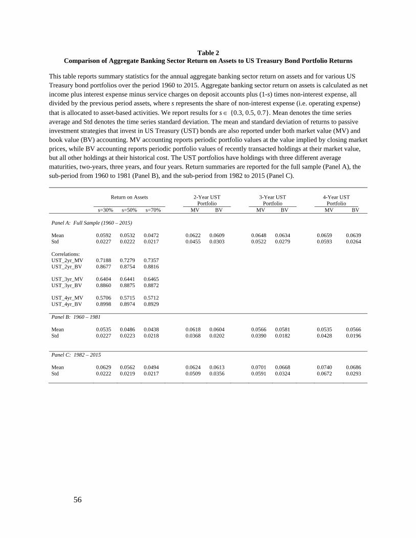
56

Table 2 Comparison of Aggregate Banking Sector Return on Assets to US Treasury Bond Portfolio Returns

This table reports summary statistics for the annual aggregate banking sector return on assets and for various US Treasury bond portfolios over the period 1960 to 2015. Aggregate banking sector return on assets is calculated as net income plus interest expense minus service charges on deposit accounts plus (1-s) times non-interest expense, all divided by the previous period assets, where s represents the share of non-interest expense (i.e. operating expense)

that is allocated to asset-based activities. We report results for s {0.3, 0.5, 0.7}. Mean denotes the time series average and Std denotes the time series standard deviation. The mean and standard deviation of returns to passive investment strategies that invest in US Treasury (UST) bonds are also reported under both market value (MV) and book value (BV) accounting. MV accounting reports periodic portfolio values at the value implied by closing market prices, while BV accounting reports periodic portfolio values of recently transacted holdings at their market value, but all other holdings at their historical cost. The UST portfolios have holdings with three different average maturities, two-years, three years, and four years. Return summaries are reported for the full sample (Panel A), the sub-period from 1960 to 1981 (Panel B), and the sub-period from 1982 to 2015 (Panel C).

Return on Assets 2-Year UST

Portfolio 3-Year UST

Portfolio 4-Year UST

Portfolio

s=30% s=50% s=70% MV BV MV BV MV BV Panel A: Full Sample (1960 – 2015) Mean 0.0592 0.0532 0.0472 0.0622 0.0609 0.0648 0.0634 0.0659 0.0639 Std 0.0227 0.0222 0.0217 0.0455 0.0303 0.0522 0.0279 0.0593 0.0264 Correlations: UST_2yr_MV 0.7188 0.7279 0.7357 UST_2yr_BV 0.8677 0.8754 0.8816 UST_3yr_MV 0.6404 0.6441 0.6465 UST_3yr_BV 0.8860 0.8875 0.8872 UST_4yr_MV 0.5706 0.5715 0.5712 UST_4yr_BV 0.8998 0.8974 0.8929 Panel B: 1960 – 1981 Mean 0.0535 0.0486 0.0438 0.0618 0.0604 0.0566 0.0581 0.0535 0.0566 Std 0.0227 0.0223 0.0218 0.0368 0.0202 0.0390 0.0182 0.0428 0.0196 Panel C: 1982 – 2015 Mean 0.0629 0.0562 0.0494 0.0624 0.0613 0.0701 0.0668 0.0740 0.0686 Std 0.0222 0.0219 0.0217 0.0509 0.0356 0.0591 0.0324 0.0672 0.0293

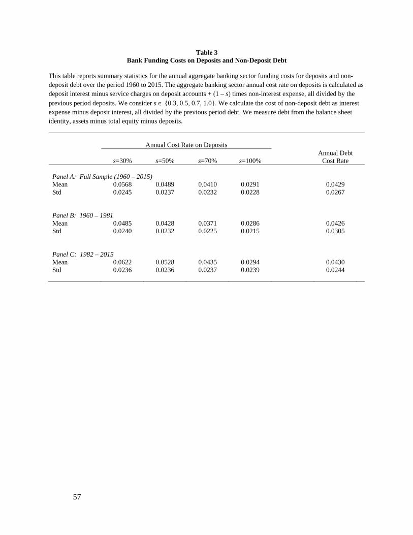
57

Table 3 Bank Funding Costs on Deposits and Non-Deposit Debt

This table reports summary statistics for the annual aggregate banking sector funding costs for deposits and non-deposit debt over the period 1960 to 2015. The aggregate banking sector annual cost rate on deposits is calculated as deposit interest minus service charges on deposit accounts + (1 – s) times non-interest expense, all divided by the

previous period deposits. We consider s {0.3, 0.5, 0.7, 1.0}. We calculate the cost of non-deposit debt as interest expense minus deposit interest, all divided by the previous period debt. We measure debt from the balance sheet identity, assets minus total equity minus deposits.

Annual Cost Rate on Deposits

s=30% s=50% s=70% s=100% Annual Debt

Cost Rate

Panel A: Full Sample (1960 – 2015) Mean 0.0568 0.0489 0.0410 0.0291 0.0429 Std 0.0245 0.0237 0.0232 0.0228 0.0267 Panel B: 1960 – 1981 Mean 0.0485 0.0428 0.0371 0.0286 0.0426 Std 0.0240 0.0232 0.0225 0.0215 0.0305 Panel C: 1982 – 2015 Mean 0.0622 0.0528 0.0435 0.0294 0.0430 Std 0.0236 0.0236 0.0237 0.0239 0.0244

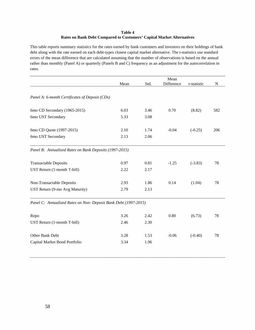
58

Table 4 Rates on Bank Debt Compared to Customers’ Capital Market Alternatives

This table reports summary statistics for the rates earned by bank customers and investors on their holdings of bank debt along with the rate earned on each debt-types closest capital market alternative. The t-statistics use standard errors of the mean difference that are calculated assuming that the number of observations is based on the annual rather than monthly (Panel A) or quarterly (Panels B and C) frequency as an adjustment for the autocorrelation in rates.

Mean Std. Mean

Difference t-statistic N

Panel A: 6-month Certificates of Deposit (CDs)

6mo CD Secondary (1965-2015) 6.03 3.46 0.70 (8.82) 582

6mo UST Secondary 5.33 3.08

6mo CD Quote (1997-2015) 2.10 1.74 -0.04 (-0.25) 206

6mo UST Secondary 2.13 2.06

Panel B: Annualized Rates on Bank Deposits (1997-2015)

Transactable Deposits 0.97 0.81 -1.25 (-3.83) 78

UST Return (1-month T-bill) 2.22 2.17

Non-Transactable Deposits 2.93 1.86 0.14 (1.04) 78

UST Return (9-mo Avg Maturity) 2.79 2.13

Panel C: Annualized Rates on Non- Deposit Bank Debt (1997-2015)

Repo 3.26 2.42 0.80 (6.73) 78

UST Return (1-month T-bill) 2.46 2.30

Other Bank Debt 3.28 1.53 -0.06 (-0.40) 78

Capital Market Bond Portfolio 3.34 1.96

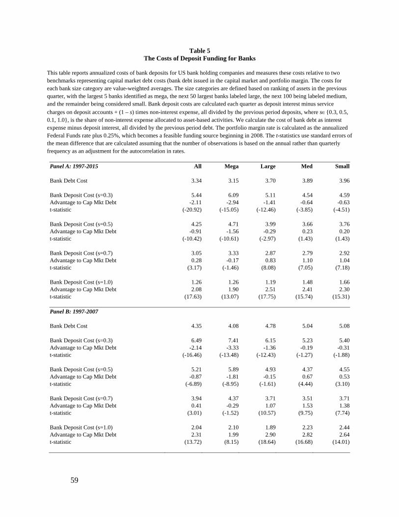
59

Table 5 The Costs of Deposit Funding for Banks

This table reports annualized costs of bank deposits for US bank holding companies and measures these costs relative to two benchmarks representing capital market debt costs (bank debt issued in the capital market and portfolio margin. The costs for each bank size category are value-weighted averages. The size categories are defined based on ranking of assets in the previous quarter, with the largest 5 banks identified as mega, the next 50 largest banks labeled large, the next 100 being labeled medium, and the remainder being considered small. Bank deposit costs are calculated each quarter as deposit interest minus service

charges on deposit accounts + (1 – s) times non-interest expense, all divided by the previous period deposits, where s{0.3, 0.5, 0.1, 1.0}, is the share of non-interest expense allocated to asset-based activities. We calculate the cost of bank debt as interest expense minus deposit interest, all divided by the previous period debt. The portfolio margin rate is calculated as the annualized Federal Funds rate plus 0.25%, which becomes a feasible funding source beginning in 2008. The t-statistics use standard errors of the mean difference that are calculated assuming that the number of observations is based on the annual rather than quarterly frequency as an adjustment for the autocorrelation in rates.

Panel A: 1997-2015 All Mega Large Med Small Bank Debt Cost 3.34 3.15 3.70 3.89 3.96 Bank Deposit Cost (s=0.3) 5.44 6.09 5.11 4.54 4.59Advantage to Cap Mkt Debt -2.11 -2.94 -1.41 -0.64 -0.63t-statistic (-20.92) (-15.05) (-12.46) (-3.85) (-4.51) Bank Deposit Cost (s=0.5) 4.25 4.71 3.99 3.66 3.76Advantage to Cap Mkt Debt -0.91 -1.56 -0.29 0.23 0.20t-statistic (-10.42) (-10.61) (-2.97) (1.43) (1.43) Bank Deposit Cost (s=0.7) 3.05 3.33 2.87 2.79 2.92Advantage to Cap Mkt Debt 0.28 -0.17 0.83 1.10 1.04t-statistic (3.17) (-1.46) (8.08) (7.05) (7.18) Bank Deposit Cost (s=1.0) 1.26 1.26 1.19 1.48 1.66Advantage to Cap Mkt Debt 2.08 1.90 2.51 2.41 2.30t-statistic (17.63) (13.07) (17.75) (15.74) (15.31) Panel B: 1997-2007 Bank Debt Cost 4.35 4.08 4.78 5.04 5.08 Bank Deposit Cost (s=0.3) 6.49 7.41 6.15 5.23 5.40Advantage to Cap Mkt Debt -2.14 -3.33 -1.36 -0.19 -0.31t-statistic (-16.46) (-13.48) (-12.43) (-1.27) (-1.88) Bank Deposit Cost (s=0.5) 5.21 5.89 4.93 4.37 4.55Advantage to Cap Mkt Debt -0.87 -1.81 -0.15 0.67 0.53t-statistic (-6.89) (-8.95) (-1.61) (4.44) (3.10) Bank Deposit Cost (s=0.7) 3.94 4.37 3.71 3.51 3.71Advantage to Cap Mkt Debt 0.41 -0.29 1.07 1.53 1.38t-statistic (3.01) (-1.52) (10.57) (9.75) (7.74) Bank Deposit Cost (s=1.0) 2.04 2.10 1.89 2.23 2.44Advantage to Cap Mkt Debt 2.31 1.99 2.90 2.82 2.64t-statistic (13.72) (8.15) (18.64) (16.68) (14.01)

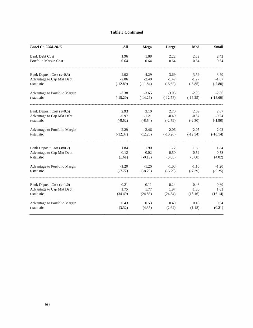
60

Table 5 Continued

Panel C: 2008-2015 All Mega Large Med Small Bank Debt Cost 1.96 1.88 2.22 2.32 2.42Portfolio Margin Cost 0.64 0.64 0.64 0.64 0.64 Bank Deposit Cost (s=0.3) 4.02 4.29 3.69 3.59 3.50Advantage to Cap Mkt Debt -2.06 -2.40 -1.47 -1.27 -1.07t-statistic (-12.89) (-11.84) (-6.62) (-6.85) (-7.80) Advantage to Portfolio Margin -3.38 -3.65 -3.05 -2.95 -2.86t-statistic (-15.20) (-14.26) (-12.78) (-16.25) (-13.69) Bank Deposit Cost (s=0.5) 2.93 3.10 2.70 2.69 2.67Advantage to Cap Mkt Debt -0.97 -1.21 -0.49 -0.37 -0.24t-statistic (-8.52) (-8.54) (-2.79) (-2.30) (-1.90) Advantage to Portfolio Margin -2.29 -2.46 -2.06 -2.05 -2.03t-statistic (-12.37) (-12.26) (-10.26) (-12.34) (-10.14) Bank Deposit Cost (s=0.7) 1.84 1.90 1.72 1.80 1.84Advantage to Cap Mkt Debt 0.12 -0.02 0.50 0.52 0.58t-statistic (1.61) (-0.19) (3.83) (3.68) (4.82) Advantage to Portfolio Margin -1.20 -1.26 -1.08 -1.16 -1.20t-statistic (-7.77) (-8.23) (-6.29) (-7.39) (-6.25) Bank Deposit Cost (s=1.0) 0.21 0.11 0.24 0.46 0.60Advantage to Cap Mkt Debt 1.75 1.77 1.97 1.86 1.82t-statistic (34.49) (24.83) (24.34) (15.16) (16.14) Advantage to Portfolio Margin 0.43 0.53 0.40 0.18 0.04t-statistic (3.32) (4.35) (2.64) (1.18) (0.21)

61

Table 6 Bank Asset Returns and Risk Premia

This table reports annualized returns on bank assets for US bank holding companies and measures these returns relative to passive maturity-matched portfolios of US Treasury bonds. The returns for each bank size category are value-weighted averages. The size categories are defined based on ranking of assets in the previous quarter, with the largest 5 banks identified as mega, the next 50 largest banks labeled large, the next 100 being labeled medium, and the remainder being considered small. Bank asset returns are calculated each quarter with various assumptions about

s, the share of non-interest expense allocated to asset-based activities, where s{0.3, 0.5, 0.1, 1.0}. The mean returns on the benchmark are accounting returns. Each month, for each size category, the benchmark portfolio invests the short-term asset share in one-month US Treasury bills and the remaining in a h-period US Treasury bond that is held until maturity, where h = 2 x the long-term average maturity of assets in that size category, with the average maturity of the bonds in the portfolio equaling h/2. The t-statistics use standard errors of the mean difference that are calculated assuming that the number of observations is based on the annual rather than quarterly frequency as an adjustment for the autocorrelation in accounting returns.

All Mega Large Medium Small

Short-term Asset Share (%) 37.69 38.81 39.04 28.73 28.3Long-term Avg Maturity in Years 4.57 3.82 5.22 5.73 5.26Loans to Assets (%) 46.3 38.98 53.25 61.03 63.69

US Treasury Benchmark Return 3.94 3.72 3.99 4.26 4.27

Bank Asset Return (s=0.3) 3.86 3.85 3.98 3.65 3.72Average Risk Premium 0.02 0.23 0.09 -0.51 -0.46t-statistic (0.14) (1.37) (0.56) (-2.91) (-3.18)

Bank Asset Return (s=0.5) 3.37 3.37 3.47 3.20 3.25Average Risk Premium -0.47 -0.25 -0.43 -0.97 -0.92t-statistic (-3.35) (-1.55) (-2.63) (-5.62) (-6.35)

Bank Asset Return (s=0.7) 2.89 2.90 2.95 2.74 2.79Average Risk Premium -0.95 -0.73 -0.95 -1.42 -1.39t-statistic (-6.57) (-4.48) (-5.69) (-8.41) (-9.44)

Bank Asset Return (s=1.0) 2.16 2.18 2.17 2.05 2.09Average Risk Premium -1.68 -1.44 -1.72 -2.11 -2.08t-statistic (-10.77) (-8.56) (-9.86) (-12.65) (-13.90)

62

Appendix

A. Data: Reporting requirements for form FR Y-9C are related to asset size and have changed over time. Specifically, in March 2006, the asset-size reporting requirement was increased from $150M to $500M, and in March 2015, it was increased from $500M to $1B. To create a more consistent sample over our sample period, we require banks to have assets exceeding a size cutoff rule defined as follows: $1B in March 2015 deflated at the quarterly rate of 1.5%. Additionally, we restrict the sample to US banks with deposits equaling at least 20% of assets. This results in an average quarterly sample size of nearly 600 BHCs that is roughly constant through time. Despite the size-based sample restrictions, the resulting sample is heavily tilted towards small banks. Most banks are three orders of magnitude smaller than the largest three banks. The following exhibit shows the size distribution of the bank sample with categories based on average ln asset values measured over 2004-2005.

Exhibit A: Size Distribution of US Bank Holding Companies Based on Average Quarterly Assets (2004-2005).

Size Category Count Mean Min Max Share

Small

499 1,310,176 528,473 5,017,250 9%Medium 72 13,643,268 5,088,496 46,675,000 13%Large 14 152,525,893 49,987,500 478,875,000 29%Mega 3 1,224,125,000 1,083,625,000 1,455,000,000 49%