Journal of Technical Analysis (JOTA). Issue 54 (2000, Summer)
37
SM A Publication of Summer-Fall 2000 ● Issue 54 MARKET TECHNICIANS ASSOCIATION, INC. One World Trade Center ● Suite 4447 ● New York, NY 10048 ● 212/912-0995 ● Fax: 212/912-1064 ● e-mail: [email protected] ● www.mta.org A Not-For-Profit Professional Organization ● Incorporated 1973 MTA JOURNAL
-
Upload
beniamin-paylevanyan -
Category
Economy & Finance
-
view
153 -
download
7
Transcript of Journal of Technical Analysis (JOTA). Issue 54 (2000, Summer)

SM
A Publication of
Summer-Fall 2000 ● Issue 54
MARKET TECHNICIANS ASSOCIATION, INC.One World Trade Center ● Suite 4447 ● New York, NY 10048 ● 212/912-0995 ● Fax: 212/912-1064 ● e-mail: [email protected] ● www.mta.org
A Not-For-Profit Professional Organization ● Incorporated 1973
MTAJOURNAL

MTA JOURNAL • Summer-Fall 2000 2
THE MTA JOURNAL – TABLE OF CONTENTS
SUMMER - FALL 2000 • ISSUE 54
12345
MTA JOURNAL EDITORIAL STAFF 3
ABOUT THE MTA JOURNAL 4
MTA MEMBER AND AFFILIATE INFORMATION 5
1999-2000 BOARD OF DIRECTORS AND MANAGEMENT COMMITTEE 6
EDITORIAL COMMENTARYADDRESS TO MTA 25TH ANNIVERSARY SEMINAR – MAY 2000 – “LIVING LEGENDS” PANEL 7
Robert J. Farrell
EXPLOITING VOLATILITY TO ACHIEVE A TRADING EDGE: MARKET-NEUTRAL/DELTA-NEUTRALTRADING USING THE PRISM TRADING SYSTEMS 9
Jeff Morton, M.D., CMT
MECHANICAL TRADING SYSTEM VS. THE SP 100 INDEX: CAN A MECHANICAL TRADING SYSTEMBASED ON THE FOUR WEEK RULE BEAT THE SP 100 INDEX? 13
Art Ruszkowski, CMT, M.Sc.
SCIENCE IS REVEALING THE MECHANISM OF THE WAVE PRINCIPLE 19
Robert R. Prechter, Jr., CMT
TESTING THE EFFICACY OF THE NEW HIGH/NEW LOW INDEX USING PROPRIETARY DATA 25
Richard T. Williams, CFA, CMT
BIRTH OF A CANDLESTICK - USING GENETIC ALGORITHM TO IDENTIFY USEFUL 31CANDLESTICK REVERSAL PATTERNS
Jonathan T. Lin, CMT

MTA JOURNAL • Summer-Fall 2000 3
EDITOR
Henry O. Pruden, Ph.D.Golden Gate University
San Francisco, California
ASSOCIATE EDITORS
David L. Upshaw, CFA, CMT Jeffrey Morton, M.D.Lake Quivira, Kansas PRISM Trading Advisors
Missouri City, Texas
Connie Brown, CMTAerodynamic Investments Inc.
Pawley's Island, South Carolina
John A. Carder, CMTTopline Investment Graphics
Boulder, Colorado
Ann F. Cody, CFAHilliard Lyons
Louisville, Kentucky
Robert B. PeirceCookson, Peirce & Co., Inc.Pittsburgh, Pennsylvania
Charles D. Kirkpatrick, II, CMTKirkpatrick and Company, Inc.
Chatham, Massachusetts
John McGinley, CMTTechnical Trends
Wilton, Connecticut
Cornelius LucaBridge Information Systems
New York, New York
Theodore �E. Loud, CMTTel Advisor Inc. of Virginia
Charlottesville, Virginia
Michael J. Moody, CMTDorsey, Wright & Associates
Pasadena, California
Richard C. Orr, Ph.D.ROME Partners
Marblehead, Massachusetts
Kenneth G. Tower, CMTUST Securities
Princeton, New Jersey
J. Adrian Trezise, M. App. Sc. (II)Consultant to J.P. Morgan
London, England
PRODUCTION COORDINATOR
Barbara I. GompertsFinancial & Investment Graphic Design
Marblehead, Massachusetts
PUBLISHER
Market Technicians Association, Inc.One World Trade Center, Suite 4447
New York, New York 10048
MANUSCRIPT REVIEWERS
THE MTA JOURNAL
SUMMER - FALL 2000 • ISSUE 54

MTA JOURNAL • Summer-Fall 2000 4
A NOTE TO AUTHORS ABOUT STYLE
You want your article to be published. The staff of the MTA Journal wants to help you. Our commongoal can be achieved efficiently if you will observe the following conventions. You'll also earn thethanks of our reviewers, editors, and production people.
1. Send your article on a disk. When you send typewritten work, please use 8-1/2" x 11" paper. DOUBLE-SPACE YOUR TEXT. If you use both sides of the paper, take care that it is heavy enough to avoidreverse-side images. Footnotes and references should appear at the end of your article.
2. Submit two copies of your article.3. All charts should be provided in camera-ready form and be properly labeled for text reference. Try
to avoid using the words "above" or "below," but rather, Chart A, Table II, etc. when referring to yourgraphics.
4. Greek characters should be avoided in the text and in all formulae.5. Include a short (one paragraph) biography. We will place this at the end of your article upon
publication. Your name will appear beneath the title of your article.We will consider any article you send us, regardless of style, but upon acceptance, we will ask you to
make your article conform to the above conventions.For a more detailed style sheet, please contact the MTA Office, One World Trade Center, Suite 4447,
New York, NY 10048.
Mail your manuscripts to:Dr. Henry O. Pruden
Golden Gate University536 Mission Street
San Francisco, CA 94105-2968
The Market Technicians Association Journal is pub-
lished by the Market Technicians Association, Inc.,
(MTA) One World Trade Center, Suite 4447, New
York, NY 10048. Its purpose is to promote the inves-
tigation and analysis of the price and volume activi-
ties of the world's financial markets. The MTA Jour-
nal is distributed to individuals (both academic and
practitioner) and libraries in the United States,
Canada, Europe and several other countries. The
MTA Journal is copyrighted by the Market Technicians
Association and registered with the Library of Con-
gress. All rights are reserved.
ABOUT THE MTA JOURNAL
DESCRIPTION OF THE MTA JOURNAL

MTA JOURNAL • Summer-Fall 2000 5
Members Affiliates■ Invitation to MTA educational meetings ■■ ■■
■ Receive monthly MTA newsletter ■■ ■■
■ Receive MTA Journal ■■ ■■
■ Use of MTA library ■■ ■■
■ Participate on various committees ■■ ■■
■ Colleague of IFTA ■■ ■■
■ Eligible to chair a committee ■■
■ Eligible to vote ■■
Annual subscription to the MTA Journal for nonmembers: $50 (minimum two issues).
Single issue of the MTA Journal (including back issues): $20 each for members and affiliates and
$30 for nonmembers.
✔ ✔
✔ ✔
✔ ✔
✔ ✔
✔ ✔
✔ ✔
✔ ■■
✔ ■■
MARKET TECHNICIANS ASSOCIATION, INC.MEMBER AND AFFILIATE INFORMATION
MEMBER
Member category is available to those "whose professional efforts are spent practicing financial technicalanalysis that is either made available to the investing public or becomes a primary input into an activeportfolio management process or for whom technical analysis is a primary basis of their investment decision-making process." Applicants for Member must be engaged in the above capacity for five years and must besponsored by three MTA Members familiar with the applicant's work.
AFFILIATE
Affiliate status is available to individuals who are interested in technical analysis, but who do not fullymeet the requirements for Member, as stated above; or who currently do not know three MTA members forsponsorship. Privileges are noted below.
DUES
Dues for Members and Affiliates are $200 per year and are payable when joining the MTA and thereafterupon receipt of annual dues notice mailed on July 1. College students may join at a reduced rate of $50 withthe endorsement of a professor.
APPLICATION FEES
Applicants for Member will be charged a onetime, nonrefundable application fee of $25; no fee forAffiliates.
BENEFITS OF THE MTA

MTA JOURNAL • Summer-Fall 2000 6
Director: PresidentPhilip B. Erlanger, CMT
Phil Erlanger Research Co. Inc.978/263-2536
Fax: 978/266-1104E-mail: [email protected]: Vice President
Richard A. DicksonScott & Stringfellow Inc.
804/780-3292Fax: 804/643-9327
E-mail: [email protected]: Secretary
Bruno DiGiorgiLowry's Reports Inc.
561/842-3514Fax: 561/842-1523
E-mail: [email protected]: Treasurer
Andrew BekoffBloomberg Financial Markets
212/495-0558Fax: 212/809-9143
E-mail: [email protected]: Past President
Dodge Dorland, CMTLANDOR Investment Management
212/737-1254Fax: 212/861-0027
E-mail: [email protected]
Bruce M. Kamich, CMTwallstreetREALITY.com, Inc.
732/463-8438Fax: 732/463-2078
e-mail: [email protected]
Charles Kirkpatrick II, CMTKirkpatrick & Co.
508/945-3222Fax: 508/945-8064
E-mail: [email protected]
Philip J. Roth, CMTMorgan Stanley Dean Witter
212/761-6603Fax: 212/761-0471
E-mail: [email protected]
Kenneth G. Tower, CMTUST Securities Corp.
609/734-7747Fax: 609/520-1635
E-mail: [email protected]
2000-2001 BOARD OF DIRECTORS AND MANAGEMENT COMMITTEEOF THE MARKET TECHNICIANS ASSOCIATION, INC.
Management Committee(4 Officers, Past President and Committee Chairs)
AccreditationDavid L. Upshaw, CFA, CMT
913/268-4708Fax: 913/268-7675
E-mail: [email protected]
Neal Genda, CMTCity National Bank
310/888-6416Fax: 310/888-6388
E-mail: [email protected] of Knowledge
John C. Brooks, CMTYelton Fiscal Inc.
770/645-0095Fax: 770/645-0098
E-mail: [email protected]
TBADistance LearningRichard A. Dickson
Scott & Stringfellow Inc.804/780-3292, Fax: 804/643-9327
E-mail: [email protected]
Philip J. Roth, CMTMorgan Stanley Dean Witter
212/761-6603Fax: 212/761-0471
E-mail: [email protected] & StandardsLisa M. Kinne, CMT
Salomon Smith Barney212/816-3796
Fax: 212/816-3590E-mail: [email protected]
FoundationBruce M. Kamich, CMT
732/463-8438Fax: 732/463-2078
e-mail: [email protected] LiaisonMike Epstein
NDB Capital Markets Corp.617/753-9910
Fax: 617/753-9914E-mail: [email protected]
Internship CommitteeJohn Kosar, CMT
Bridge Information Services312/930-1511
Fax: 312-454-3465E-mail: [email protected]
Board of Directors(4 Officers, 4 Directors & Past President)
Journal�Henry (Hank) O. PrudenGolden Gate University
415/442-6583Fax: 415/442-6579
E-mail: [email protected]
Daniel L. Chesler, CTA, CMT561/793-6867
Fax: 561/791-3379E-mail: [email protected]
MembershipLarry Katz
Market Summary & Forecast805/370-1919
Fax 805/777-0044E-mail: [email protected]
NewsletterMichael N. Kahn
Bridge Information Systems212/372-7541
E-mail: [email protected]
Rick BensignorMorgan Stanley Dean Witter
212/761-6148Fax: 212/761-0471
E-mail: [email protected] (NY)Bernard Prebor
MCM MoneyWatch212/908-4323
Fax: 212/908-4331E-mail: [email protected]
RegionsM. Frederick Meissner
404/875-3733E-mail: [email protected]
RulesGeorge A. Schade, Jr., CMT
602/542-9841Fax: 602/542-9827
E-mail: [email protected]
Nina G. CooperPendragon Research, Inc.
815/244-4451Fax: 815/244-4452
E-mail: [email protected]
MTA JOURNAL • Summer-Fall 2000 7
ADDRESS TO MTA 25TH ANNIVERSARY SEMINAR – MAY 2000“LIVING LEGENDS” PANEL
Robert J. Farrell
[Editor's Note: At the 25th Anniversary Seminar in May 2000 inAtlanta, Georgia, Bob Farrell was a member of a panel called The LivingLegends: A tribute to, and remarks by, the eight winners of the MTA An-nual Award. The winners were: Art Merrill, Hiroshi Okamoto, RalphAcampora, Bob Farrell, Don Worden, Dick Arms, Alan Shaw, and JohnBrooks and all were in attendance. The panel was hosted by your editor,Henry Pruden. The following is the text from Bob Farrell's presentation:]
I appreciate being included in this 25th anniversary year forMTA Seminars. I also appreciate being one of the living recipients
of the annualaward. I remem-ber participatingin the first semi-nar as part of whatwas called the 1-2-3 panel for thefirst time. Institu-tional Investormagazine had in-cluded a markettiming category inits annual All-American Re-search Team polland Don Hahn,
Stan Berge and I were those chosen. That was an indication ofgreater institutional recognition of market analysis and timing. Be-fore the great Bear Market of 1972-74, technical analysis was mostlyregarded with suspicion by professionals. Institutional portfoliomanagers generally denigrated its importance even though in ev-ery meeting I had with them, they all carried chart books. The bigbreakthrough came, however, after so many of them got hurt inthe 1972-74 Bear Market. They started asking how could we haveanticipated the collapse of the nifty-fifty and most other stocks. Theythen began to notice that many market analysts and technicianshad issued warnings about the coming debacle. From then on,they started paying more attention. But just as they did not careabout technical timing at the top of the bull market in the late1960s, by the mid-1970s they wanted to hear more about how toavoid the next bear market. In fact, the Financial Analysts Federa-tion asked me to speak at their annual conference in New York in1975 on using technical tools to avoid the next bear market. WhatI chose to speak about was how to use market timing tools to helpidentify where to be invested for the coming long-term bull mar-ket. It seemed clear to me bear markets of the 1974 intensity didnot come along often and set the stage for new long bull runs.They wanted to me to talk about the past instead of the future.
When I chose to be a market analyst instead of a security analystin the early 1960s, I soon realized that what I needed as a goal wasprofessional recognition. I also realized that it could only comefrom institutions as their dominance was growing in the market.But I knew most portfolio manager's eyes glazed over when I spokeof technical indicators or they were outright hostile to technicians.
So, I came up with a plan. I incorporated more long-term trendand cycle work in my analysis so portfolio managers could look atmy analysis as something beyond short-term trading. I also real-ized I could get their attention by giving them fundamental rea-sons for the conclusions I had arrived at using market indicators.Then I figured out that if I wanted to have impact, effective com-munication was everything. Of course, I had to be right a goodpercentage of the time and make sense, but the ability to write andspeak in a common sense style without arrogance was crucial togetting their attention.
I also realized, as I am sure many of you have figured out, thatmost professional money managers have strong views that you arenot going to change in a single meeting or with a single report.When I got a conviction about a sector or a market change, I knewit had to offer more than a conclusion or opinion. We had to sup-ply information and present it logically to prove a point. Today,there is more information available more quickly than ever beforebut, interestingly, results of most managers are still worse than apassive index. Most want and need to be told which information isimportant. One of the things I capitalized on was the idea that Ihad information not available elsewhere, i.e., Merrill Lynch inter-nal transaction figures. We, in fact, applied the term sentimentanalysis to our figures back in the mid 1960s and used them toadvantage as contrary indicators. Even though they were only onetool, they gave us an edge in supplying unique information to cli-ents. Today, of course, many firms have such data and it is lessunique.
I don't believe in us versus them when it comes to technical analysisand fundamental analysis. The goal is to come up with profitableideas, not whose tools are best. Nevertheless, I had one chance toturn the tables on fundamental security analysts which I enjoyedimmensely. When I went to Columbia Business School in 1955 toget a Master's in Investment Finance, I had both Ben Graham andDavid Dodd as professors. As you know, they were the originalvalue investors who wrote the bible of fundamental analysis called,"Security Analysis." Published in 1934, there was a 50th anniver-sary seminar in 1984 at Columbia to which I was invited as a speaker.When the Dean first invited me, I asked him incredulously, "Doyou know what I do?" Even though he understood that most tech-nical analysis was poles apart from the fundamental value trainingof Graham & Dodd, he said, "Just tell us how they influenced you."I was the last speaker on the all-day program which included War-ren Buffet, Mario Gabelli and others, and I felt very intimidated.But I decided to try a different approach and gave a speech en-titled, Why Ben Graham Was A Closet Technician. Surprisingly, it waswell received. I cited many references he made to the characteris-tics of a market top and his references to measures of speculation.
The fact that I was rated number one in 16 of the 17 years Icompeted in the Institutional Investor All-Star Research poll as ChiefMarket Analyst was not because I was more right than anybody else.I did have a good platform at Merrill Lynch but not everybody atMerrill was ranked #1 either. I think it was my ability to communi-cate what was happening or changing in the markets with an his-

MTA JOURNAL • Summer-Fall 2000 8
torical perspective in a form that mostly fundamental clients couldunderstand. I never talked down to them and always had a sectoropinion that I emphasized where my conviction level was high. Ithought they usually took away something useful from my presen-tation even if they disagreed with some of the general conclusions.
As a result of the integration of fundamental reasoning to backup technical conclusions, I became less regarded as a technicianand more as a market strategist who used historical precedent andtechnical tools. I have never liked the term technician because it istoo limiting and am very much in favor of finding another way todescribe what we do. We study so many things such as price trends,momentum, money flows, cycles and waves, investor behavior andsentiment, supply-demand changes, volume relationships, insideractivity, monetary policy and historical precedent. We have a broadfield of study that has grown more inclusive with time and the com-puter age. It is just not adequately summed up in the term techni-cian. At Merrill Lynch, we use the broader term of market analystto avoid the limiting label of technician. Despite all the attemptsat upgrading and professionalizing our craft by our association, westill have the press calling technicians sorcerers, elves, entrail read-ers and other denigrating terms. We have come a long way, but wehave not shaken the negative image of the past that goes with theterm technician, particularly with the press. You may disagree oreven not care, but experience tells me to emphasize our broaderrange of skills.
I am impressed with the advanced techniques being used to ana-lyze the market data and the progress made in working with theFinancial Analysts Federation and the academic community. Thereis much more substance in our craft as a result of your efforts. Nev-ertheless, the world at large needs to be educated. Investor's Busi-ness Daily does an excellent job of explaining how to use technicaltools and integrate technical and fundamental information on anongoing, real-time basis. We should use this model as an organiza-tion and have our members publish regular educational articles inthe mainstream press or on a net website. We have created excel-lent professional credentials over the years. Now we need to mar-ket our profession – if not as technicians, perhaps as market behav-ioral strategists or market timing and behavioral strategists. Youdeserve recognition for your broader range of skills as well as yourability to provide profitable market and stock conclusions.
Thank you for inviting me.
ROBERT J. FARRELL
Bob Farrell is Senior Investment Advisor of Merrill Lynch,Pierce, Fenner & Smith, Inc., the nation’s largest securitiesfirm, and one of Wall Street’s most highly respected stock mar-ket analysts.
He had been named Number One in the Market Timingcategory of Institutional Investor’s annual “All-American Re-search Team” poll for 16 years prior to assuming his new role.
Bob has spent his entire business career with Merrill Lynch.As Manager of Market Analysis, he pioneered the use of senti-ment figures using Merrill Lynch internal data. His “WeeklyMarket Commentary,” published since 1970, was followed bythousands of professional money managers in this country andabroad.
In his current role as Senior Investment Advisor, he hasbeen writing quarterly on longer-term theme changes in themarket. He will continue advising clients on market strategiesimplementing themes.
Bob was a charter member of the Market Technicians Asso-ciation and its first president from 1972-1974. Bob was alsothe recipient of the MTA Annual Award in 1988. In 1993 hewas inducted into the Wall Street Week Hall of Fame.
He was graduated from Manhattan College in 1954 with aBBA in Economics & Finance, and received an MS in invest-ment finance from the Columbia Graduate School of Busi-ness in 1955.
MTA JOURNAL • Summer-Fall 2000 9
PurposeThis study was designed to evaluate the theoretical returns for a
simple non-directional option strategy initiated after a sudden andsignificant volatility implosion of an underlying stock.
Methods and MaterialsThe 30 Dow Jones Industrial stocks from November 1, 1993,
through May 30, 1998, were chosen for this study. Delta neutral/gamma positive straddle positions were initiated on the openingprice of the stock after the near-term historical volatility of the stockhad significantly imploded relative to its longer-term historical vola-tility. Any signals generated in the same stock before the 6- weektermination date of a prior trade were ignored. On the date ofcalculation, the options prices were determined with the actualimplied volatility using the Black-Scholes model, assuming moder-ate slippage. All trades were equally weighted. The value of theoptions’ positions were calculated based on the closing stock priceat the 2-, 4-, and 6- week periods respectively. Two trading systemswere evaluated. In the first system (time-based system), time wasthe sole determinant used to determine when the option positionswould be closed out. In the second trading system (money man-agement system), simple money management rules were added toreduce draw-downs and to “lock-in” profits in profitable trades.Given the wide variability of brokerage fees, the results are pre-sented without commission costs deducted.
ResultsA total of 280 trades were generated between November 1, 1993,
and May 30, 1998. For the time-based trading system (trading system1), the 2-week, 4-week, and 6-week cumulative return was -191.9%,+334.7%, and -84.3% and the average return per trade was -0.69%,+1.20%, and -0.30% respectively. For the money managementtrading system (trading system 2), the 4-week and 6-week cumulativereturns were +993.4%, and +1188.6% and the average return pertrade was +3.55% and +4.25% respectively. The use of a simplemoney management system significantly reduced the draw-downsof the system.
ConclusionsThe simple time-based volatility trading strategy produced a
positive return holding the options for four weeks. This simplestraddle-based options strategy had significant draw-downs thatpreclude it as a viable trading strategy without modifications. Theaddition of some very simple money management rules significantlyimproved the returns while simultaneously decreasing the draw-downs. This volatility-based, market-neutral, delta-neutral (gammapositive) trading strategy yielded a very substantial positive returnacross a large number of large-cap stocks and across a broad fiveyear period. These results demonstrate the potential positive re-turns that can be obtained from a market-neutral/delta-neutralstrategy. The benefit of a market-neutral strategy as demonstratedhere is of significant importance to institutional portfolio manag-ers in search of non-correlated asset classes.
INTRODUCTION
For options-based trading, the price action of any freely-tradedasset (e.g., stocks, futures, index futures, etc.) can be grouped intothree generic categories (however defined by the trader): (a) bull-ish price action; (b) bearish price action; (c) congestion/tradingrange price action. Specific options-based strategies can be imple-mented which result in profits if any two out of the three outcomesunfold. For example, the purchase of both call and put options onthe same underlying asset for the same strike price and same expi-ration date is termed a “straddle” position (e.g., buying XYZ $100strike March 1999 call and put options = XYZ $100 March 1999straddle). This straddle position can be profitable if either (a) or(b) quickly occur with significant magnitude (i.e., price volatility)prior to option expiration. In this sense, a straddle trade is non-directional since it can profit in both bull and bear moves.
Price volatility can be described by several common technicalindicators including ADX, average-true-range, standard deviation,and statistical volatility (also called historical volatility). Volatilityhas been observed to be “mean-reverting.” Periods of abnormallyhigh or low short-term price volatility are followed by price volatil-ity that is closer to the long-term price volatility of the underlyingasset.(1,3) A short-term drop in price volatility (volatility implosion)can be reliably expected to be followed by a sudden volatility in-crease (volatility explosion). Connors, et. al. have shown that mul-tiple days of short-term volatility implosion is a predictor of a strongprice move.(1,2)
The volatility implosion does not predict the direction of theimpending price move, but only that there is a high probabilitythat the underlying asset is going to move away from its currentprice and by a significant amount. In addition, the volatility implo-sion does not predict when (how quickly) the explosion price movewill develop. We can predict which direction the price of the stock,commodity, or market is not going to move with a high degree ofprobability. It most likely will not move side-ways indefinitely. Know-ing this, one can devise a trading strategy that is able to profit, or atleast not lose money, if the stock moves quickly higher or lowersuch as the straddle strategy earlier described above.
In the option straddle strategy described above (e.g., XYZ $100March 1999 straddle), as the price of the underlying asset movesaway from the option's strike price in either direction, the optionthat is gaining in value will increase at a greater rate than the op-posing option that is losing value. The position is said to be gammapositive in both directions. The straddle will lose if the price of theasset stays at or near the strike prices of the options, i.e. the stockmoves side-ways. The straddle position deteriorates because ofcontinued decrease in the volatility of the underlying asset, plusthe time-decay value of the option as it approaches expiration.
This study was designed to explore the potential investment re-turns that could be obtained using the basic option straddle strat-egy. At PRISM Trading Advisors, Inc., this strategy has been suc-cessfully implemented to generate superior returns at lower riskthan traditional investment portfolio benchmarks.
EXPLOITING VOLATILITY TO ACHIEVE A TRADING EDGE:Market-Neutral/Delta-Neutral Trading Using
the PRISM Trading Systems
Jeff Morton, MD, CMT
1

MTA JOURNAL • Summer-Fall 2000 10
METHODS AND MATERIALS
System 1 (Time-Based Strategy)To test the robustness of this trading strategy, the Dow 30 Indus-
trial stocks from November, 1, 1993, through May 31, 1998, werechosen for this study. They were chosen because they are a well-known group of stocks that have been designed to represent themarket at large. Volatility is defined by the price statistical volatil-ity formula: s.v. = s.d.{log(c/c[1]),n} * square-root (365). Statisti-cal (or historical) price volatility can be descriptively defined asthe standard deviation of day-to-day price change using a log-nor-mal distribution and stated as an annualized percentage. Detailedinformation on statistical volatility is available from the refer-ences.(1,2,3)
■ Rule 1: 6-day s.v. is 50% or less than the 90-day s.v.■ Rule 2: 10-day s.v. is 50% or less than the 90-day s.v.■ Rule 3: Both rule #1 and rule #2 must be satisfied to
initiate the trade. Thus in this study, a volatility implosion was defined as when
the 6-day and 10-day historical volatilities were 50% or less thanthe 90-day historical volatility. When this condition is met, a signalto initiate a straddle position was taken the following trading day.The Black-Scholes model was used to calculate the options pricesthat were used to establish the straddle positions. The openingprice of the stock, the actual implied volatility, and the yield of the90-day U.S. Treasury Bill were used to calculate the price of theoptions. The professional software package OpVue 5 version 1.12(OpVue Systems International) was used to calculate the prices ofthe options assuming a moderate amount of slippage. For the pur-poses of this analysis, it was assumed that each trade was equallyweighted and that an equal dollar amount was invested into eachtrade. Based on the closing stock price, the value of the optionstraddle positions were then calculated using the same methoddescribed above after 2 weeks, 4 weeks, and 6 weeks respectively.Any trading signals generated in a stock with a current open op-tion straddle position before the end of the 6-week open trade pe-riod were ignored. To minimize the effect of time decay and vola-tility, options with greater than 75 days to expiration were used toestablish the straddle positions. The positions were closed out atthe end of the 6-week time period with more than 30 days left untilexpiration. To further minimize the effect of volatility, options werepurchased “at or near the money.” Given the current large vari-ability of brokerage fees, the results were calculated without de-ducting commission costs.
System 2 (Money Management Strategy)A second trading strategy was explored. It was identical to the
first trading strategy except a set of simple money managementrules were added. The rules were designed to 1) cut losses short,2) allow profits to run, and 3) lock in profits.■ Rule #1: A position was closed immediately if a 10% loss oc-
curred.■ Rule #2: If a 5% profit (or greater) was generated, then a trail-
ing stop of one-half (50%) of the maximum open profit achievedby the position was placed and the position closed if the 50%trailing stop was violated.
■ Rule #3: If neither rule #1 or #2 was violated then the positionwas closed out after either 4 weeks or 6 weeks.
RESULTS
System 1 (Time-Based Strategy)A total of 280 trades were generated between November 1, 1993
and May 30, 1998. Numerous parameters of the 280 trades wereanalyzed. The results are summarized in Table 1. The 2-week, 4-week, and 6-week cumulative returns were +191.9%, +334.7%, and-84.3% respectively and are shown in Figure 1. The return of theDJIA over the same time period was +241.8% (3,680.59 to 8,899.95).The maximum draw-downs for the 2-week, 4-week, and 6-week se-ries were, -424.3%, (November 12, 1993 - April 28, 1995), -450.8%(November 8, 1993 - May 17, 1995), and -763.3% (December 6,1993 - May 19, 1995). The maximum draw-ups for the 2-week, 4-week, and 6-week series were, +373.9% (April 7, 1995 - July 1, 1997),+933.2% (April 18, 1995 - November 11, 1997), and +948.2% (April7, 1995 - November 17, 1997).
System 2 (Money Management Strategy)A total of 280 trades were generated between November 1, 1993
and May 30, 1998. Numerous parameters of the 280 trades wereanalyzed. The results are summarized in Table 2. The 4-week, and6-week cumulative returns were +993.4%, and +1188.6% respec-tively, and are shown in Figure 2. The return of the DJIA over thesame time period was +241.8% (3,680.59 to 8,899.95). The maxi-mum draw-downs for the 4-week and 6-week series were -188.1%,(August 5, 1994 - February 23, 1995) and -246.2% (August 5, 1994- February 23, 1995). The maximum draw-ups for the 4-week and6-week series were +641.4% (September 20, 1996 - October 20, 1997)and +704.1% (September 20, 1996 - October 20, 1997).
DISCUSSION
It has been observed that short-term volatility will have a ten-dency to revert back to its longer-term mean.(1,3) Connors et.al.(1)
have published the Connors-Hayward Historical Volatility Systemand showed that when the ratio of the 10-day versus the 100-dayhistorical volatilities was 0.5 or less, there was a tendency for strongstock price moves to follow.
In this study, PRISM Trading Advisors, Inc., have confirmed thephenomenon of volatility mean reversion by presenting the firstlarge scale option-based analysis while maintaining a strict market-neutral/delta-neutral (gamma positive) trading program. We haveshown that a significant price move occurs 75% of the time follow-ing a short-term volatility implosion (as defined in the Methodsand Materials section).
For this analysis we chose a relatively straightforward strategy:to purchase a straddle. A straddle is the proper balance of put andcall options that produce a trade with no directional bias. A straddleis said to be “delta neutral” and will generate the same profit whetherthe underlying asset’s price moves higher or lower. As the assetprice moves away from its initial price one option will increase invalue while the other opposing option will decrease in value. Aprofit is generated because the option that is increasing in valuewill increase in value at a faster rate than the opposing option isdecreasing in value. The straddle is said to be “gamma positive” inboth directions.
This option strategy has a defined maximum risk of the tradethat is known at the initiation of the trade. This maximum risk ofloss is limited to the initial purchase costs of the straddle (premiumcosts of both put and call options). There is no margin call withthis straddle strategy. There is an additional way that this strategycan profit. Since the options are purchased at the time there has

MTA JOURNAL • Summer-Fall 2000 11
(Over)
been an acute rapid decrease in volatility, one should theoreticallybe purchasing “undervalued” options. As the price of the assetsubsequently experiences a sharp price move, there will be an asso-ciated increase in volatility which will increase the value of all theoptions that make-up the straddle position. The side of the straddlewhich is increasing in value will increase at an even faster rate, whilethe opposite side of the straddle which is decreasing in value willdecrease in value at a slower rate. So as to not further complicatethe analysis, the exit strategy for the first system (time-based strat-egy) for this study was even more basic using a time-stop exit crite-ria.
Prior to the study, it was our impression that a 4-week time pe-riod would be the most optimal of the three. This is what was seen.The 4-week exit produced a positive return over the study period(334.7%). However, the use of a 2-week time-stop was frequentlynot sufficient time to allow for the anticipated price move. Notethat in Figure 1, the 2-week maximum open-profit draw-up was sig-nificantly less than the draw-ups for both the 4-week and 6-weektime-stops (373.9% vs. 933.2% and 948.2% respectively). The 6-weeks strategy was too long, allowing for substantially greater maxi-mum draw-down secondary to the adverse effects of time decay,volatility, and price regression back toward the stock’s initial start-ing price that eroded the value to the straddle position when com-pared to the 2-week and 4-week strategies. All other aspects of thetrades of the three exit strategies were similar. There were no sig-nificant differences in the percentage of wining/losing trades ornumber of consecutive winning or losing trades.
A second system using a simple set of money management ruleswas tested (money management system). These rules were designedto close-out non-performing trades early before they could turninto large losses and kept performing positions open as long asthey continued to generate profits. These goals were accomplishedby closing out any position if its value decreased to 90% of its ini-tial value (10% loss). A position with open profits had a 50% trail-ing stop of the maximum open profit achieved by the position atanytime open profits exceeded 5%. If neither of these two condi-tions occurred, the position was closed out at the end of six weeks.
As predicted, the 6-week money management strategy producedboth a greater total return (+993.4% versus 1,188.6%) and a slightlygreater maximum draw-down than the 4-week money managementstrategy. By closing positions when a loss of 10% had occurred, wewere able to significantly decrease the amount of losses incurred.This is evidenced by the maximum draw-down for the 6-weekpositions being decreased significantly from (-763.3%) to (-246.2%) employing no money management versus implementingthe above money management rules. Also the total returns weremarkedly improved with the total return increasing from (-84.3%)to (+1188.6%).
While the first trading system (time-based strategy) study dem-onstrated that this trading strategy with a 4-week time-stop exit pro-duced a positive return, it is not sufficient as a stand-alone systemfor real-time trading. It does, however, indicate that this strategycan be used as the foundation to design a viable trading systemthat can capture the majority of the gains while simultaneously elimi-nating the majority of the loses. There are almost an infinite num-ber of possibilities one could explore to achieve this goal.
The second method, and the one explored in this paper, wasthe application of a simple set of money management rules. Asdiscussed above, this dramatically improved the overall returns whilesimultaneously decreasing the draw-downs experienced in the firststrategy (time-based strategy). Other possibilities include the ad-dition of a second entry filter such as a momentum indicator like
the RSI, ROC or MACD indicator. One could design a more so-phisticated exit strategy such as exiting the position if the stockprice exceeds a predetermined price objective as defined by pricechannels, parabolic functions, etc. An additional possibility wouldbe to re-establish a nondirectional option’s position at a predeter-mined price objective, thereby “locking in” all the profits gener-ated up to that point. The myriad of options-based strategies avail-able to adjust back to a delta neutral position based on technicalindicators and predetermined price objectives are beyond the scopeof this paper.
Although both systems had positive expectations based on 280trades, there are several limitations of the study design. Althoughmoderate slippage was used in all the calculations, the robustnessof this study might have been improved if access to real-time stockoption bid-ask prices were available for all of the trades investi-gated. Unfortunately, such a large, detailed database is not readilyavailable. Given that the real-time bid-ask prices were not avail-able, the use of the Black-Scholes formula with the known histori-cal inputs (stock price, implied volatility, 90-day T-Bill yield) is anacceptable alternative thereby minimizing any pricing differencesbetween the actual and theoretical option prices systematicallythroughout the time period used in the study.
The current study revealed that a simple straddle options-basedstrategy designed to exploit a sudden implosion of a stock’s volatil-ity with time as the only existing criteria produced draw-downs thatpreclude it as a viable trading strategy in its own right. However,this simple strategy had a positive expectation of generating supe-rior returns, and therefore can be used as the basis to develop trad-ing strategies capable of producing superior returns without theneed to correctly predict the direction of a given stock, commod-ity, or market being traded. The addition of some simple moneymanagement rules dramatically improved the overall returns whilesimultaneously decreasing the excessive draw-downs that plaguedthe original trading strategy, thereby transforming it into a appli-cable trading system for every day use. This volatility-based, delta-neutral strategy also is independent of market direction. A mar-ket-neutral strategy and portfolio may be considered as a separateasset class by portfolio managers in the efficient allocation of theirclients’ investment portfolios to boost returns while simultaneouslydecreasing their clients risk exposure.
In conclusion, this is the first large-scale trading research studyto be shared with the trading public that clearly demonstrated howthe phenomenon of price volatility mean-reversion can be exploitedby using an options-based delta-neutral approach. Price, time andvolatility factors using options-based strategies to further maximizepositive expectancy represent active areas of real-time trading re-search at PRISM Trading Advisors, Inc. These results will be thesubject of future articles.
REFERENCES
1. Connors, L. A., and Hayward, B.E., Investment Secrets of a HedgeFund Manager, Probus Publishing, 1995.
2. Connors, L. A: Professional Traders Journal, Oceanview FinancialResearch, Malibu, CA. March 1996, Volume 1, Issue 1.
3. Natenberg, S., Option Volatility and Pricing. Advanced Trading Strat-egies and Techniques, McGraw Hill, 1994.

MTA JOURNAL • Summer-Fall 2000 12
TABLE 1
System 1 (Time-Based System)
2 Week 4 Week 6 Week
Total Return -191.9% +334.7% -84.3%
Average Return per Trade -0.69% +1.20% -0.30%
Maximum Draw-Up +373.9% +933.2% +948.2%
Maximum Draw-Down -424.3% -450.8% -763.3%
Total # Winning Trades 91 106 100
Total # Break Even Trades 4 0 3
Total # Losing Trades 185 174 177
Max. # of Consecutive Wins 7 5 5
Max. # of Consecutive Loses 14 9 13
Greatest Gain in One Trade +87.8% +132.1% +109.0%
Greatest Loss in One Trade -48.0% -51.8% -59.0%
Figure 1
System 1 (Time-Based System)
TABLE 2
System 2 (Money Management System)
4 Week 6 Week
Total Return +993.4% +1188.6%
Average Return per Trade +3.55% +4.25%
Maximum Draw-up +641.4% +704.1%
Maximum Draw-Down -188.1% -246.2%
Total # Winning Trades 120 117
Total # Break Even Trades 0 2
Total # Losing Trades 160 161
Max. # Consecutive Wins 6 7
Max. # Consecutive Loses 8 9
Greatest Gain in One Trade +132.1% +109.0%
Greatest Loss in One Trade -10.0% -10.0%
Figure 2
System 2 (Money Management System)
JEFF MORTON, MD, CMT
Jeff Morton is Chief Technical Analyst & Executive VicePresident at PRISM Trading Advisors (Electronic SignatureOnly). He received his bachelor’s degree from Stanford Uni-versity Medical School in 1981 and his Medical Degree fromthe Yale School of Medicine in 1985. He began his career as atechnical analysts in 1992 as a consultant for Schea CapitalManagement. In 1995, he helped start PRISM Trading Advi-sors, Inc. a Houston, Texas based proprietary trading firm.His major areas of expertise include options strategies, volatil-ity trading, and trading strategies based on ADX, ATR, point& figure charting. His other duties at PRISM Trading Advi-sors, Inc. include compliance/due diligence, trader education,and journal publications. Dr. Morton is very active in theMTA. He currently is serving as an associate editor of the MTAJournal, and on the accreditation committee.

MTA JOURNAL • Summer-Fall 2000 13
PREFACE
In their quest to outperform the Index, equity fund managersmust solve a four-piece puzzle: which stocks should they buy, whenshould they buy them, when should they sell them and how much capitalshould they allocate to each stock. The performance of different fundmanagers varies greatly. Some are able to outperform the Index,and others cannot. This paper investigates the question of whethertechnical analysis in its most simplistic form along with simplemoney management can be used to outperform the Index.
THE FOUR-WEEK RULE
Most market technicians will agree that the simplest technicalmarket analysis rule is the Four-Week Rule. The Four-Week Rule(4WR) was originally developed for application to futures marketsby Richard Donchian, and can be expressed as follows:
Cover shorts and go long when the price exceeds the highs of thefour preceding full calendar weeks and conversely liquidate longsand go short when the price falls below the lows of the four preced-ing full calendar weeks.
The rationale behind this rule is that the four-week or 20-daytrading cycle is a dominant cycle that influences all markets.
For the purpose of further discussion, let’s modify the Four-Week Rule system as follows:
Buy if the price exceeds the highs of the four preceding full calendarweeks and liquidate open positions when the price falls below thelows of the four preceding full calendar weeks.
With this modification, the 4WR – (no shorts) system can beeasily applied by many equity fund managers because very few ofthem can go short.
Let us formally define our modified mechanical system:
System Code: NS-20BS-EQ (No Shorts, 20 days for Buy andSell Rules, Equally Allocate Capital)
1. Money management rule - Equal allocation ruleUse $100,000 of capital into one hundred S&P 100 Index stocks,allocating an equal amount of money into each stock ($1000).
2. Technical analysis rule - BuyBuy a stock if its closing price is higher than the high of last 20trading days.
3. Technical analysis rule - SellSell a stock if its close price is lower than the low of last 20 trad-ing days
4. Money management rule - Redistribute profits equallyIf the profit from the sale of a stock is greater than the initialallocation of capital to this stock, then that profit is equally dis-tributed among all stocks which are in a potential Buy position.
5. Money management rule - Earn interest on cashAll cash on hand earns fix rate interest @ 5% per annum.
6. Money management rule - Transaction costsA fixed transaction cost of $50 is applied to each transaction(this cost represents a fair average of commissions and slippage).
A custom computer software was designed and created to testthis system in the time frame from January 1, 1984 to January 1,1989. During this time frame the following performance statisticswere calculated for NS-20BS-EQ system and were compared to theperformance statistics of the Index (S&P 100) with a “Buy-and-HoldStrategy.”
Performance Statistics MeasuredThe following performance statistics were measured for each
case (definitions are included in Appendix 1):■ Average Annual Compounded Return (R)■ Sharpe Ratio (SR)■ Return Retracement Ratio (RRR)■ Maximum Loss (ML)
ResultsDays used for
System� Time Frame� Money Allocation� Buy and Sell rules�
NS-20BS-EQ� 01/01/1984 - 01/01/1989 Equal 20�
System� IndexAverage Annual Compounded Return 7.58% 9.00%��
Sharpe Ratio� 4.15% 3.85%��
Return Retracement Ratio� 0.45 0.34��
Maximum Loss� 0.36� 0.58��
It is clear that the above system is performing less than the “Buy-and-Hold Strategy” of S&P 100 Index.
There are several choices to improve performance of the sys-tem by modifying system parameters. The most natural change isto search for better performance by modifying the number daysused for the Buy and Sell rules. The performance of the NS-xBS-EQ system where x is the number of days for Buy and Sell rules wastested for x between 10 days and 90 days. Results of the test areprovided in the Appendix 2.1.
Testing proved that the best performing system was the one with50 days used for the Buy and Sell rules.
ResultsDays used for
System� Time Frame� Money Allocation� Buy and Sell rules�
NS-50BS-EQ 01/01/1984 - 01/01/1989 Equal� 50��
System IndexAverage Annual Compounded Return� 7.70%� 9.00%��
Sharpe Ratio 4.49% 3.85%��
Return Retracement Ratio 0.42 0.34��
Maximum Loss� 0.40� 0.58��
Still the performance of the above system is not very impres-sive, so let’s consider further research. Let’s modify Rule 1 fromthe system definition and replace it by following rule:1A. Money management rule - Proportional allocation rule
Use $100,000 of capital into one hundred S&P 100 Index stocks,allocating money into each stock according to its percentageparticipation in the index at the starting date of the testing pe-riod (January 1, 1984).
MECHANICAL TRADING SYSTEM VS. THE S&P 100 INDEXCan a Mechanical Trading System Based on the
Four-Week Rule Beat the S&P 100 Index?
Art Ruszkowski, CMT, M.Sc.
2
MTA JOURNAL • Summer-Fall 2000 14
So we consider the new system:
System Code: NS-xBS-P (No Shorts, x Days for Buy and SellRules, Proportionally Allocate Capital)
The new system consists of Rule 1A and Rules 2-6.The performance of the NS-xBS-P system where x is the num-
ber of days for Buy and Sell rules was tested for x between 10 daysand 90 days. Results of the test are provided in the Appendix 2.2.
Testing proved that the best-performing system was one with 50days used for Buy and Sell rules.
ResultsDays used for
System� Time Frame� Money Allocation� Buy and Sell rules�
NS-50BS-P� 01/01/1984 - 01/01/1989 Proportional� 50��
System� IndexAverage Annual Compounded Return� 10.57%� 9.00%��
Sharpe Ratio� 4.44% 3.85%��
Return Retracement Ratio� 0.51 0.34��
Maximum Loss� 0.48 0.58��
The last system outperforms the S&P100 “Buy-and-Hold Strat-egy” but let’s consider further research. So far modifications werelimited to systems with different number of days for the Buy andSell rule and for using different initial allocations of the capital –equal and proportional. Let’s consider the following hybrid of theoriginal NS-20BS-EQ system – by replacing Rule 3 with followingnew rule:3B. Money management Stop Loss Rule - Sell losing positions
Sell a stock if it is losing more than y% of its buy price, where yis a system parameter
Let’s name this system:
System Code: NS-xB-P-Sy (No Shorts, x Days for Buy Rule,Proportionally Allocate Capital, – Sell When Drops y%)
Only systems with proportionally allocated capital are analyzeddue to the fact that they perform better than equally allocated onesin a considered period of time. The performance of the NS-xB-P-Sy system where x is the number of days for Buy rule was tested forx between 10 days and 90 days and for y between 10% and 70%.Results of the test are provided in the Appendix 3.
Testing of systems NS-xB-P-Sy proved that the best performingsystem was one with 50 days used for Buy rule and 25% moneymanagement stop loss rule.
ResultsMoney Days used % Loss used
System� Time Frame� Allocation� for Buy in Rule 3B
NS-50B-P-S25� 01/01/1984 - 01/01/1989 Proportional� 50� 25%��
System� IndexAverage Annual Compounded Return� 14.78%� 9.00%��
Sharpe Ratio� 4.48%� 3.85%��
Return Retracement Ratio� 0.52� 0.34��
Maximum Loss� 0.64� 0.58��
The last system which is the result of several cycles of modifica-tions to the initial 4WR outperforms the S&P100 “Buy-and-HoldStrategy” by a good margin. To find out how time-stable the abovesystem was, a blind test was conducted.
Blind Test Results: System (NS-50B-P-S25)The system was tested in a new time period (between January 1,
1989 and January 1, 1994). Here is the comparison of market sta-tistics between the Index and the NS-50B-P-S25 system in the timeframe from January 1, 1989 to January 1, 1994.
System� IndexAverage Annual Compounded Return� 13.88%� 10.00%��
Sharpe Ratio� 5.47%� 6.92%��
Return Retracement Ratio� 0.68� 0.59��
Maximum Loss� 0.49� 0.40��
Comparing these values, we see that the system still outper-formed the Index in respect to the Average Annual CompoundedReturn (by 40%) and the Return Retracement Ratio, but margin-ally under-performed with the other two statistics. This can be ex-plained by comparing the monthly DMI readings in the time pe-riod of 1984-1989 and 1989-1994. In the first time period, the stan-dard 14-month Directional Movement Index (DMI) was well above25 (a strong trending market); however, in the second time pe-riod, the DMI was only marginally above 25 (a weak trending mar-ket). So in such a time period, a trend following system doesn’tdisplay as impressive results.
GRAPHS
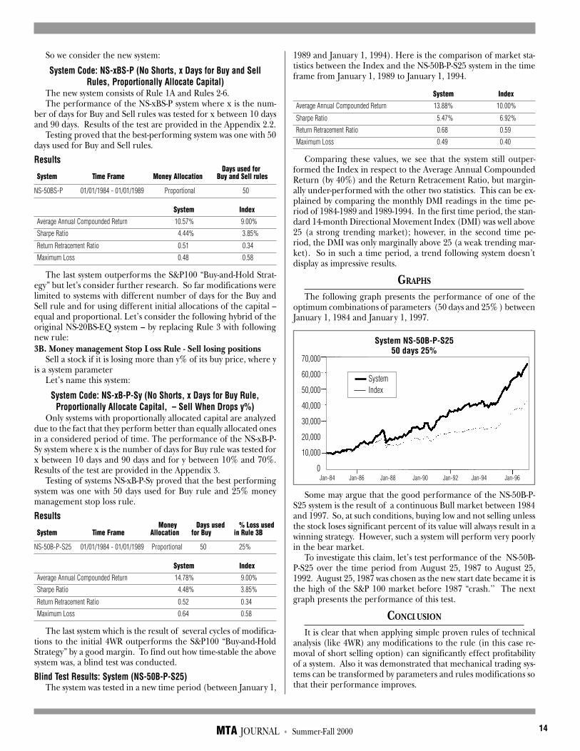
The following graph presents the performance of one of theoptimum combinations of parameters (50 days and 25% ) betweenJanuary 1, 1984 and January 1, 1997.
Some may argue that the good performance of the NS-50B-P-S25 system is the result of a continuous Bull market between 1984and 1997. So, at such conditions, buying low and not selling unlessthe stock loses significant percent of its value will always result in awinning strategy. However, such a system will perform very poorlyin the bear market.
To investigate this claim, let’s test performance of the NS-50B-P-S25 over the time period from August 25, 1987 to August 25,1992. August 25, 1987 was chosen as the new start date became it isthe high of the S&P 100 market before 1987 “crash.’’ The nextgraph presents the performance of this test.
CONCLUSION
It is clear that when applying simple proven rules of technicalanalysis (like 4WR) any modifications to the rule (in this case re-moval of short selling option) can significantly effect profitabilityof a system. Also it was demonstrated that mechanical trading sys-tems can be transformed by parameters and rules modifications sothat their performance improves.
System NS-50B-P-S2550 days 25%
70,000
60,000
50,000
40,000
30,000
20,000
10,000
0
SystemIndex
Jan-84 Jan-86 Jan-88 Jan-90 Jan-92 Jan-94 Jan-96

MTA JOURNAL • Summer-Fall 2000 15
One very interesting observation worth further study is the factthat the large difference in performance was affected by the amountof money allocated into each stock. This is due to fact that the S&P100 Index is a capitalization-weighted index of 100 stocks. Thecomponent stocks are weighted according to the total market valueof their outstanding shares. The impact of the component’s pricechange is proportional to the stock’s total market value, which isthe share price times the number of shares outstanding. In otherwords, the S&P 100 Index can be considered as a relative-strengthbased index. An index-based capital allocation system (NS-50B-P-S25) performs best and gives an objective measure of the validityof its trading rules as well as its money management rules when itsperformance is compared to the performance of the Index. Sys-tems with sound trading and money management rules, as well ascapital-allocation based on relative strength should, in general,outperform both the index and equally-allocated systems.
It is worth observing that the proportionally-allocated systemoutperformed the equally-allocated system and the Index duringthe tested time periods regardless whether during those periodsthe Large Cap outperformed the Small Cap or vice versa.
BIBLIOGRAPHY
i John. J. Murphy, Technical Analysis of the Futures Markets, NewYork Institute of Finance,1986.
ii Jack D. Schwager, Schwager on Futures - Technical Analysis, JohnWiley & Sons, Inc., 1996.
iii Carla Cavaletti, Trading Style Wars, Futures, July 1997.�
APPENDIX 1
Glossary of Terms:Mechanical Trading System: A set of rules that can be used to gen-erate trade signals and trading performed according to the rulesof mechanical system. Primary benefits of mechanical trading sys-tems are elimination of emotions from trading, and consistency ofapproach and risk management. Mechanical trading systems canbe classified as Trend-Following (initiating a position with thetrend), and Counter-Trend (initiating a position in the oppositedirection to the trend). Trend following systems can be dividedinto fast and slow. Fast – a more sensitive system responds quicklyto signs of trend reversal and will tend to maximize profit on validsignals, but also generate far more false signals. A good trend fol-lowing system should not be too fast or too slow. ii �
Trading according to signals generated by mechanical tradingsystem is called systematic trading which is opposite to discretion-ary trading. Discretionary traders claim that emotions, which areexcluded from systems trading, offer an edge. On the contrary,
systematic traders favor backtesting, analyzing patterns and elimi-nating emotions. According to Barclay Trading Group Ltd., overthe last ten years systematic traders have yielded higher annual re-turns than discretionary traders six times. iii �Optimization of the trading system: The process of finding thebest performing parameter set for a given system. The underlyingpremise of optimization is that the parameter set must work notonly in its initial time frame but any time frame. Almost any me-chanical system can be optimized in a way that it will show positiveresults in any given period of time. ii
Parameter: A value that can be freely assigned in the trading sys-tem in order to vary the timing of signals. iiParameter Set: Any combination of parameter values. ii
Parameter Stability: The goal of optimization is to find broad re-gions of parameter values with good system performance, insteadonly one parameter which can represent an isolated set of marketconditions. ii
Time Stability: In the case of positive performance of the mechani-cal system in a specific time frame, it should be analyzed in differ-ent time frames to make sure the good performance is not depen-dent only on the initial time frame. ii
Blind Simulation: This is the test of an optimized parameter set ina different time frame to see if the good results reoccur.Average Parameter Set Performance: The complete universe ofparameter sets is defined before any simulation. Simulations arethen run for all the selected parameter sets, and the average ofthese is used as an indication of the system’s potential performance.ii
Average Annual Compounded Return: R = exp(1/N(ln(E) - ln(S)) - 1S - starting equityE - ending equityN - number of years ii
Return Retracement Ratio: (RRR) = R/AMRR - average annual compounded returnAMR - average maximum retracement for each data point. Using
drawdowns (the worst at each given point in time) to measurerisk, the risk component of RRR (AMR) comes closer to de-scribing risk than standard deviation. n
AMR=1/n(Σ MRi) i=1MRi=max(MRPPi,MRSLi)
MRPPi=(PEi - Ei)/PeiMRSLi=(Ei - MEi)/Ei-1Ei - equity at the end of month i,PEi - peak equity on or prior to month i,Ei-1 - equity at the end of month prior to month i,MEi - minimum equity on or subsequent to month i.
RRR represents better return/risk measure than Sharpe ratio.ii
Sharpe Ratio: SR=E/sdvE - expected returnSdv - standard deviation of returns.ii
Expected Net Profit Per Trade: ENPPT= P*AP - L*AL,P - percent of total trades that are profitableL - percent of total trades that are in net lossAP - average net profit of profitable tradesAL - average net loss of losing trade.ii
Maximum Loss: ML= max(MRSLi)i<=n, this represent worse-casepossibilityii
Trade-Based Profit/Loss Ratio: TBPLR= P*AP/L*ALii
4WR_NS_B50_P_M2550 days 25%
20,000
15,000
10,000
5,000
0
SystemIndex
Aug-87 Aug-88 Aug-89 Aug-90 Aug-91

MTA JOURNAL • Summer-Fall 2000 16
APPENDIX 3To find the best performing system we follow procedure:1. For each column in first table select five best-performing rows.2. Select best-performing rows from each column in the second
table only if the row was selected in first table.3. Repeat step two for each subsequent table.4. Select optimal cell from still left cells.
System Money Allocation Sell Rule Start End��
NS-xB-P-Sy Proportional No 01/01/1984 01/01/1989��
This table shows the Average Annual Compounded Return (R)in %. The columns are the percentages used in the Sell Losing Posi-tions Rule and the rows are the number of days used in the Buy rule.
� 10%� 15%� 20%� 25%� 30%� 35%� 40%� 50%� 60%� 70%10� 14.47� 14.43� 14.84� 14.82� 14.95� 15.04� 15.05� 15.11� 15.17� 15.16��
20� 13.79� 14.40� 14.76� 14.92� 14.95� 15.09� 15.14� 15.22� 15.26� 15.25��30� 13.96� 14.57� 14.68� 14.81� 14.94� 15.08� 15.13� 15.20� 15.26� 15.25��40� 13.83 � 14.03� 14.36� 14.56� 14.68� 14.70� 14.78� 14.87� 14.92� 14.94� �
50 � 13.74� 14.00� 14.23� 14.56� 14.68� 14.67� 14.78� 14.88� 14.92� 14.94��
60 � 13.32� 13.94� 14.24� 14.38� 14.33� 14.52� 14.51� 14.73� 14.73� 14.50��
70� 13.59� 14.08� 14.38 � 14.35� 14.39� 14.42� 14.40� 14.63� 14.62� 14.65��
80 13.30� 14.08� 14.18� 14.16� 14.22� 14.21� 14.21� 14.42� 14.41� 14.43
90 13.23� 14.00� 14.10� 14.07� 14.17� 14.12� 14.16� 14.36� 14.35� 14.37��
This table shows the Sharpe Ratio in %. The columns are thepercentages used in the Sell Losing Positions Rule and the rows arethe number of days used in the Buy rule.
10%� 15%� 20%� 25%� 30%� 35%� 40%� 50%� 60%� 70%��10 4.32� 4.29� 4.38� 4.38� 4.41� 4.42� 4.43� 4.44� 4.43� 4.43
20 � 4.22� 4.34� 4.42� 4.45� 4.47� 4.48� 4.49� 4.49� 4.49� 4.49� �
30� 4.33 � 4.45� 4.46� 4.49� 4.49� 4.53� 4.53� 4.53� 4.53� 4.5340� 4.29 � 4.37� 4.41� 4.46� 4.46� 4.47� 4.47� 4.47� 4.46� 4.46� �
50 � 4.31� 4.37� 4.43� 4.47� 4.47� 4.48� 4.48� 4.48� 4.47� 4.47
60 � 4.25� 4.37� 4.43� 4.45� 4.45� 4.47� 4.47� 4.45� 4.45� 4.45��
70 � 4.33� 4.37� 4.43 � 4.43� 4.43� 4.45� 4.45� 4.43� 4.43� 4.43��
80� 4.28� 4.36� 4.39� 4.39� 4.39� 4.40� 4.40� 4.39� 4.39� 4.39
90 � 4.32� 4.38� 4.39� 4.39� 4.39� 4.40� 4.40� 4.38� 4.38� 4.38��
This table shows the Return Retracement Ratio. The columnsare the percentages used in the Sell Losing Positions Rule and therows are the number of days used in the Buy rule.
� 10%� 15%� 20%� 25% 30% 35% 40% 50% 60% 70%��
10 � 0.49� 0.48� 0.50� 0.49� 0.49� 0.50� 0.50� 0.50� 0.50� 0.50
20 � 0.49� 0.49� 0.50� 0.50� 0.50� 0.50� 0.50� 0.50� 0.50� 0.50
30� 0.51 � 0.51� 0.51� 0.50� 0.51 �0.51� 0.51� 0.51� 0.51� 0.51
40� 0.51� 0.50� 0.51� 0.50� 0.51� 0.51� 0.51� 0.51� 0.51� 0.51
50� 0.51 � 0.51� 0.51� 0.51� 0.52� 0.51� 0.52� 0.52� 0.52� 0.5260 � 0.51� 0.51� 0.51� 0.51� 0.51� 0.51� 0.51� 0.52� 0.52� 0.52
70 � 0.52� 0.53� 0.53 � 0.53� 0.53� 0.53� 0.53� 0.54� 0.54� 0.54
80 � 0.51� 0.53� 0.53� 0.53� 0.53� 0.53� 0.53� 0.54� 0.54� 0.54
90 � 0.51� 0.53� 0.53� 0.53� 0.53� 0.53� 0.53� 0.54� 0.54� 0.54
APPENDIX 2.1
Results for NS-xBS-EQ where x represents number of daysused in Buy and Sell rules, x>=10 and x<=90
To find optimal number of days used in Buy and Sell rules fol-low procedure:1. In each column select five best performing results (according
to the column definition. So for example in the case of theaverage annual compounded return, we select five highest num-bers, but in the case of maximum loss five lowest numbers).Mark the results by bold typeface.
2. Find the rows which are marked in each column - mark the rowsby italic typeface.
3. From selected rows choose one with the optimal results.Number of Average Sharpe Return Expected Net Trade Based MaximumDays for Buys Annual Ratio Retracement Profit Per Profit Loss Loss (ML)and Sell Compounded in % Ratio Trade Ratio in %Rules Return (%) (ENPPT)($) (TBPLR)
10 3.93� 2.82� 0.30� 96.20� 1.34� 2620� 7.58� 4.15� 0.45� 296.53� 1.81� 36� �30 � 8.46� 4.27� 0.48� 471.96� 2.05� 40� �40� 8.04 � 4.36� 0.44� 559.21� 2.09� 40 �
50 � 7.70� 4.49� 0.42� 638.58 � 2.13� 40� �60 � 7.84� 4.50� 0.43� 770.62� 2.30� 40��
70 � 7.76 4.60 0.42 859.30 2.41 41
80 � 7.59� 4.64� 0.40� 930.93� 2.49 � 41�
90� 7.56� 4.64� 0.39� 1011.86� 2.59 � 42��
The optimal the system with 50 days used for Buy and Sell rules.
APPENDIX 2.2
Results for NS-xBS-P where x represents number of daysused in Buy and Sell rules, x>=10 and x<=90
Number of Average Sharpe Return Expected Net Trade Based MaximumDays for Buys Annual Ratio Retracement Profit Per Profit Loss Loss (ML)and Sell Compounded in % Ratio Trade Ratio in %Rules Return (%) (ENPPT)($) (TBPLR)��
10 4.48� 3.07� 0.30� 109.72� 1.40� 29 �
20� 8.85� 4.18� 0.48� 361.66� 2.04� 40 � �
30 � 10.05� 4.37� 0.52� 594.16� 2.44� 44
40 � 10.15� 4.37� 0.52� 763.29� 2.73� 4650� 10.57� 4.44� 0.51� 979.46� 2.95� 48 ��60 � 10.90� 4.38� 0.53� 1206.84 � 3.43� 48��
70� 10.96 � 4.55� 0.51� 1206.84� 3.85� 49��
80 � 10.62� 4.60� 0.48� 1479.84� 3.91� 50��
90 10.30� 4.61� 0.47� 1585.23� 4.19� 50��
The optimal is the system with 50 days for Buy and Sell rules.

MTA JOURNAL • Summer-Fall 2000 17
This table shows the Expected Net Profit Per Trade (ENPPT)in $. The columns are the percentages used in the Sell Losing Posi-tions Rule and the rows are the number of days used in the Buy rule.
10%� 15%� 20%� 25%� 30%� 35%� 40%� 50%� 60%� 70%��10 3511.64� 4507.22� 5905.14� 6597.08� 7739.21� 8520.50� 8823.50� 9802.04� 10245.87 10447.28
20 3385.28� 4695.31� 5949.73� 7252.84 7716.12 8677.11 9264.20 9869.52 10502.81 10498.79
30 � 3709.77 5067.45 5923.62 7009.01 7807.08 8492.72 9224.62 9817.10 10472.16 10465.79
40 � 3805.97 4834.92 5955.58 7140.84 7725.92 8265.74 8924.55 9607.69 10041.16 10156.11
50� 3925.73 � 5107.18� 6188.47� 7345.42� 7969.82� 8372.83� 9164.75� 9608.21�10030.17�10149.77
60 � 3710.81� 5241.00� 6428.99� 7492.27� 7966.95� 8540.02� 8931.42� 9557.56� 9840.63� 9961.49
70 � 4053.34� 5541.77� 6717.81 � 7384.87� 8043.70� 8427.56� 8805.56� 9528.22� 9711.08� 9830.62
80 � 4078.14� 5771.52� 6622.01� 7355.29� 8109.93� 8316.63� 8708.21� 9420.13� 9502.17� 9619.90
90 � 4020.47 5821.46 6611.41 7275.61 8127.05 8230.48 8736.40 9347.20 9432.68 9544.71
This table shows the Maximum Loss (ML) in %. The columnsare the percentages used in the Sell Losing Positions Rule and therows are the number of days used in the Buy rule.
� 10%� 15%� 20% �25%� 30%� 35%� 40%� 50%� 60%� 70%��10� 0.65� 0.66� 0.66� 0.66� 0.66� 0.66� 0.67� 0.67� 0.67� 0.67��
20 � 0.63� 0.65� 0.65� 0.66� 0.66� 0.66� 0.66� 0.66� 0.67� 0.67��
30 � 0.62� 0.64� 0.64� 0.65� 0.65� 0.65� 0.66� 0.66� 0.66� 0.66��
40� 0.61� 0.62� 0.63� 0.64� 0.64� 0.64� 0.65� 0.65� 0.65� 0.65��
50� 0.61� 0.62� 0.63� 0.63� 0.64� 0.64� 0.64� 0.64� 0.64� 0.6460 � 0.60� 0.61� 0.62� 0.63� 0.63� 0.63� 0.63� 0.64� 0.64� 0.64��
70 � 0.60� 0.61� 0.61 � 0.62� 0.62� 0.62� 0.62� 0.62� 0.62� 0.62
80 � 0.59� 0.61� 0.61� 0.61� 0.61� 0.61� 0.61� 0.61� 0.61� 0.61
90 � 0.59� 0.60� 0.61� 0.61� 0.61� 0.61� 0.61� 0.61� 0.61� 0.61�
This table shows the Trade-Based Profit/Loss Ratio (TBPLR).The columns are the percentages used in the Sell Losing PositionsRule and the rows are the number of days used in the Buy rule.
� 10%� 15%� 20%� 25%� 30%� 35%� 40%� 50%� 60% 70%10 9.76 10.04 14.62 16.25 19.87 25.01 27.07 39.85 62.18 81.81
20 � 8.95� 11.17� 15.42� 21.44� 22.65� 26.89� 32.67� 41.55� 95.37� 93.95
30 � 10.31� 13.94� 15.41� 19.61� 22.47� 26.39� 32.00� 40.02� 93.59� 92.20
40 � 10.24� 12.44� 15.63� 20.79� 23.31� 25.28� 31.02� 37.71� 60.18� 90.27
50 10.15� 12.93� 16.78� 21.31� 24.21 � 24.91� 33.52� 38.51 61.27 93.06
60 9.11� 13.88� 19.17� 24.92� 25.00� 30.36� 33.32� 63.53� 64.58� 102.15
70 � 11.45� 16.57� 23.84 � 24.46� 27.89� 29.73� 30.79 �64.39� 63.26� 99.61
80 � 11.08� 19.83� 23.73� 24.85� 29.52� 29.36� 31.24� 66.51� 64.05� 102.01
90 � 11.36� 20.05� 24.62� 24.23� 31.79 �29.51� 33.90� 71.46� 69.73 111.06
The best performing is the system with 50 days used for Buyrule and 25% Sell Losing Position rule.�
ART RUSZKOWSKI, CMT, M.SC.Art Ruszkowski combines his strong scientific background
with knowledge and practice of technical analysis specializingin quantitive analysis, and mechanical trading system designand testing. He is currently a partner in a private investmentfund, and is responsible for development of models, studies,portfolio selections and money management strategies.
Art is a member of the MTA and the CSTA.

MTA JOURNAL • Summer-Fall 2000 18
It is one thing to say that the Wave Principle makes sense in thecontext of nature and its growth forms. It is another to postulate ahypothesis about its mechanism. The biological and behavioral sci-ences have produced enough relevant work to make a case thatunconscious paleomentational processes produce a herding im-pulse with Fibonacci-related tendencies in both individuals andcollectives. Man’s unconscious mind, in conjunction with others, isthus disposed toward producing a pattern having the properties ofthe Wave Principle.
THE PALEOMENTATIONAL HERDING IMPULSE
Over a lifetime of work, Paul MacLean, former head of the Labo-ratory for Brain Evolution at the National Institute of Mental Health,has developed a mass of evidence supporting the concept of a“triune” brain, i.e., one that is divided into three basic parts. Theprimitive brain stem, called the basal ganglia, which we share withanimal forms as low as reptiles, controls impulses essential to sur-vival. The limbic system, which we share with mammals, controlsemotions. The neocortex, which is significantly developed only inhumans, is the seat of reason. Thus, we actually have three con-nected minds: primal, emotional and rational. Figure 1, fromMacLean’s book, The Triune Brain in Evolution,1 roughly shows theirphysical locations.
The neocortex is involved in the preservation of the individualby processing ideas using reason. It derives its information fromthe external world, and its convictions are malleable thereby. Incontrast, the styles of mentation outside the cerebral cortex areunreasoning, impulsive and very rigid. The “thinking” done by thebrain stem and limbic system is primitive and pre-rational, exactlyas in animals that rely upon them.
The basal ganglia control brain functions that are often termedinstinctive: the desire for security, the reaction to fear, the desire toacquire, the desire for pleasure, fighting, fleeing, territorialism,migration, hoarding, grooming, choosing a mate, breeding, theestablishment of social hierarchy and the selection of leaders. Morepertinent to our discussion, this bunch of nerves also controls co-ordinated behavior such as flocking, schooling and herding. All
these brain functions insure lifesaving or life-enhancing actionunder most circumstances and are fundamental to animal motiva-tion. Due to our evolutionary background, they are integral tohuman motivation as well. In effect, then, portions of the brain are“hardwired for certain emotional and physical patterns of reaction”2
to insure survival of the species. Presumably, herding behavior, whichderives from the same primitive portion of the brain, is similarlyhardwired and impulsive. As one of its primitive tools of survival,then, emotional impulses from the limbic system impel a desireamong individuals to seek signals from others in matters of knowl-edge and behavior, and therefore to align their feelings and con-victions with those of the group.
There is not only a physical distinction between the neocortexand the primitive brain but a functional dissociation between them.The intellect of the neocortex and the emotional mentation of thelimbic system are so independent that “the limbic system has thecapacity to generate out-of-context, affective feelings of convictionthat we attach to our beliefs regardless of whether they are true or false.”3
Feelings of certainty can be so overwhelming that they stand fast inthe face of logic and contradiction. They can attach themselves toa political doctrine, a social plan, the verity of a religion, the suretyof winning on the next spin of the roulette wheel, the presumedpath of a financial market or any other idea.4 This tendency is sopowerful that Robert Thatcher, a neuroscientist at the Universityof South Florida College of Medicine in Tampa, says, “The limbicsystem is where we live, and the cortex is basically a slave to that.”5
While this may be an overstatement, a soft version of that depic-tion, which appears to be a minimum statement of the facts, is thatmost people live in the limbic system with respect to fields of knowl-edge and activity about which they lack either expertise or wisdom.
This tendency is marked in financial markets, where most peoplefeel lost and buffeted by forces that they cannot control or foresee.In the 1920s, Cambridge economist A.C. Pigou connected coop-erative social dynamics to booms and despression.6 His idea is thatindividuals rountinely correct their own errors of thought whenoperating alone but abidicate their responsibility to do so in mat-ters that have strong social agreement, regardless of the egregious-ness of the ideational error. In Pigou's words,
Apart altogether from the financial ties by which different busi-nessmen are bound together, there exists among them a certain mea-sure of psychological interdependence. A change of tone in one partof the business world diffuses itself, in a quite unreasoning man-ner, over other and wholly disconnected parts.7
“Wall Street” certainly shares aspects of a crowd, and there isabundant evidence that herding behavior exists among stock mar-ket participants. Myriad measures of market optimism and pessi-mism8 show that in the aggregate, such sentiments among both thepublic and financial professionals wax and wane concurrently withthe trend and level of the market. This tendency is not simply fairlycommon; it is ubiquitous. Most people get virtually all of their ideasabout financial markets from other people, through newspapers,television, tipsters and analysts, without checking a thing. Theythink, “Who am I to check? These other people are supposed to beexperts.” The unconscious mind says: You have too little basis uponwhich to exercise reason; your only alternative is to assume that theherd knows where it is going.
SCIENCE IS REVEALING THE MECHANISM OF THEWAVE PRINCIPLE
Robert R. Prechter, Jr., CMT3
Figure 1The Three Sections of the Triune Brain
Source: The Triune Brain in Evolution

MTA JOURNAL • Summer-Fall 2000 19
In 1987, three researchers from the University of Arizona andIndiana University conducted 60 laboratory market simulations us-ing as few as a dozen volunteers, typically economics students butalso, in some experiments, professional businessmen. Despite giv-ing all the participants the same perfect knowledge of coming divi-dend prospects and then an actual declared dividend at the end ofthe simulated trading day, which could vary more or less randomlybut which would average a certain amount, the subjects in these ex-periments repeatedly created a boom-and-bust market profile. The extrem-ity of that profile was a function of the participants’ lack of experi-ence in the speculative arena. Head research economist Vernon L.Smith came to this conclusion: “We find that inexperienced trad-ers never trade consistently near fundamental value, and most com-monly generate a boom followed by a crash....” Groups that haveexperienced one crash “continue to bubble and crash, but at re-duced volume. Groups brought back for a third trading sessiontend to trade near fundamental dividend value.” In the real world,“these bubbles and crashes would be a lot less likely if the sametraders were in the market all the time,” but novices are alwaysentering the market.9
While these experiments were conducted as if participants couldactually possess true knowledge of coming events and so-called fun-damental value, no such knowledge is available in the real world.The fact that participants create a boom-bust pattern anyway is over-whelming evidence of the power of the herding impulse.
It is not only novices who fall in line. It is a lesser-known factthat the vast majority of professionals herd just like the naïve ma-jority. Figure 2 shows the percentage of cash held at institutions asit relates to the level of the S&P 500 Composite Index. As you cansee, the two data series move roughly together, showing that pro-fessional fund managers herd right along with the market just asthe public does.
Apparent expressions of cold reason by professionals followherding patterns as well. Finance professor Robert Olsen recentlyconducted a study of 4,000 corporate earnings estimates by com-pany analysts and reached this conclusion:
Experts’ earnings predictions exhibit positive bias and disappoint-ing accuracy. These shortcomings are usually attributed to somecombination of incomplete knowledge, incompetence, and/or mis-representation. This article suggests that the human desire for con-
sensus leads to herding behavior among earnings forecasters.10
Olsen’s study shows that the more analysts are wrong, which isanother source of stress, the more their herding behavior increases.11
How can seemingly rational professionals be so utterly seducedby the opinion of their peers that they will not only hold, but changeopinions collectively? Recall that the neocortex is to a significantdegree functionally disassociated from the limbic system. Thismeans not only that feelings of conviction may attach to utterlycontradictory ideas in different people, but that they can do so inthe same person at different times. In other words, the same brain cansupport opposite views with equally intense emotion, depending uponthe demands of survival perceived by the limbic system. This factrelates directly to the behavior of financial market participants, whocan be flushed with confidence one day and in a state of utter panicthe next. As Yale economist Robert Schiller puts it, “You wouldthink enlightened people would not have firm opinions” about mar-kets, “but they do, and it changes all the time.”12 Throughout the herd-ing process, whether the markets are real or simulated, and whetherthe participants are novices or professionals, the general convic-tion of the rightness of stock valuation at each price level is power-ful, emotional and impervious to argument.
Falling into line with others for self-preservation involves notonly the pursuit of positive values but also the avoidance of nega-tive values, in which case the reinforcing emotions are even stron-ger. Reptiles and birds harass strangers. A flock of poultry will peckto death any individual bird that has wounds or blemishes. Like-wise, humans can be a threat to each other if there are perceiveddifferences between them. It is an advantage to survival, then, toavoid rejection by revealing your sameness. D.C. Gajdusek researched along-hidden Stone Age tribe that had never seen Western peopleand soon noticed that they mimicked his behavior; whenever hescratched his head or put his hand on his hip, the whole tribe didthe same thing.13 Says MacLean, “It has been suggested that suchimitation may have some protective value by signifying, ‘I am like you.’”He adds, “This form of behavior is phylogenetically deeply in-grained.”14
The limbic system bluntly assumes that all expressions of “I amnot like you” are infused with danger. Thus, herding and mimick-ing are preservative behavior. They are powerful because they areimpelled, regardless of reasoning, by a primitive system of menta-tion that, however uninformed, is trying to save your life.
As with so many useful paleomentational tools, herding behav-ior is counterproductive with respect to success in the world of mod-ern financial speculation. If a financial market is soaring or crash-ing, the limbic system senses an opportunity or a threat and ordersyou to join the herd so that your chances for success or survival willimprove. The limbic system produces emotions that support thoseimpulses, including hope, euphoria, cautiousness and panic. Theactions thus impelled lead one inevitably to the opposite of survivaland success, which is why the vast majority of people lose whenthey speculate.15 In a great number of situations, hoping and herd-ing can contribute to your well-being. Not in financial markets. Inmany cases, panicking and fleeing when others do cuts your risk.Not in financial markets. The important point with respect to thisaspect of financial markets is that for many people, repeated failuredoes little to deter the behavior. If repeated loss and agony cannot over-come the limbic system's impulses, then it certainly must have freerein in comparatively benign social settings.
Regardless of their inappropriateness to financial markets, theseimpulses are not irrational because they have a purpose, no matterhow ill-applied in modern life. Yet neither are they rational, as they
Figure 2
Stock Mutual Funds Cash/Assets Ratio vs. Aggregate Stock Prices
Monthly Data 12/31/65 - 12/31/98 (log scale)
Source: Ned Davis Research Data: Investment Company Institute

MTA JOURNAL • Summer-Fall 2000 20
are within men’s unconscious minds, i.e., their basal ganglia andlimbic system, which are equipped to operate without and to over-ride the conscious input of reason. These impulses, then, serverational general goals but are irrationally applied to too many spe-cific situations.
PHI IN THE UNCONSCIOUS MENTATIONAL PATTERNS
OF INDIVIDUALS AND GROUPS
At this point, we have identified unconscious, impulsive mentalprocesses in individual human beings that are involved in govern-ing behavior with respect to one’s fellows in a social setting. Is itlogical to expect such impulses to be patterned? When the uncon-scious mind operates, it could hardly do so randomly, as that wouldmean no thought at all. It must operate in patterns peculiar to it. In-deed, the limbic systems of individuals produce the same patternsof behavior over and over when those individuals are in groups.The interesting observation is how the behavior is patterned. Whenwe investigate statistical and scientific material on the subject, rareas it is, we find that our Fibonacci-structured neurons and microtubules(see “Science is Validating the Concept of the Wave Principle”)participate in Fibonacci patterns of mentation.
Perhaps the most rigorous work in this area has been performedby psychologists in a series of studies on choice. G.A. Kelly pro-posed in 1955 that every person evaluates the world around himusing a system of bipolar constructs.16 When judging others, forinstance, one end of each pole represents a maximum positive traitand the other a maximum negative trait, such as honest/dishon-est, strong/weak, etc. Kelly had assumed that average responses invalue-neutral situations would be 0.50. He was wrong. Experimentsshow a human bent toward favor or optimism that results in a re-sponse ratio in value-neutral situations of 0.62, which is phi. Nu-merous binary-choice experiments have reproduced this finding,regardless of the type of constructs or the age, nationality or back-ground of the subjects. To name just a few, the ratio of 62/38 re-sults when choosing “and” over “but” to link character traits, whenevaluating factors in the work environment, and in the frequencyof cooperative choices in the prisoner’s dilemma.17
Psychologist Vladimir Lefebvre of the School of Social Sciencesat the University of California in Irvine and Jack Adams-Webber ofBrock University corroborate these findings. When Lefebvre askssubjects to choose between two options about which they have nostrong feelings and/or little knowledge, answers tend to divide into
Fibonacci proportion: 62% to 38%. When he asks subjects to sortindistinguishable objects into two piles, they tend to divide theminto a 62/38 ratio. When subjects are asked to judge the “light-ness” of gray paper against solid white and solid black, they persis-tently mark it either 62% or 38% light,18 favoring the former. (SeeFigure 3.) When Adams-Webber asks subjects to evaluate theirfriends and acquaintances in terms of bipolar attributes, they choosethe positive pole 62% of the time on average.19 When he asks asubject to decide how many of his own attributes another shares,the average commonality assigned is 0.625.20 When subjects aregiven scenarios that require a moral action and ased what percent-age of people would take good actions vs. bad actions, their an-swers average 62%.21 “When people say they feel 50/50 on a sub-ject,” Lefebvre says, “chances are it's more like 62/38.”22
Lefebvre concludes from these findings, “We may suppose thatin a human being, there is a special algorithm for working withcodes independent of particular objects.”23 This language fits MacLean’sconclusion and LeDoux’s confirmation that the limbic system canproduce emotions and attitudes that are independent of objectivereferents in the cortex. If these statistics reveal something abouthuman thought, they suggest that in many, perhaps all, individualhumans, and certainly in an aggregate average, opinion is predis-posed to a 62/38 inclination. With respect to each individual deci-sion, the availability of pertinent data, the influence of prior expe-riences and/or learned biases can modify that ratio in any giveninstance. However, phi is what the mind starts with. It defaults to phiwhenever parameters are unclear or information insufficient foran utterly objective assessment.
This is important data because it shows a Fibonacci decision-based mentation tendency in individuals. If individual decision-making reflects phi, then it is less of a leap to accept that the WavePrinciple, which also reflects phi, is one of its products. To narrowthat step even further, we must be satisfied that phi appears in groupmentation in the real world. Does Fibonacci-patterned decision-making mentation in individuals result in a Fibonacci-patterneddecision-making mentation in collectives? Data from the 1930s andthe 1990s suggests that it does.
Lefebvre and Adams-Webber’s experiments show unequivocallythat the more individuals’ decisions are summed, the smaller is thevariance from phi. In other words, while individuals may vary some-what in the phi-based bias of their bipolar decision-making, a largesum of such decisions reflects phi quite precisely. In a real-worldsocial context, Lefebvre notes by example that the median votingmargin in California ballot initiatives over 100 years is 62%. Thesame ratio holds true in a study of all referenda in America over adecade24 as well as referenda in Switzerland from 1886 to 1978.25
In the early 1930s, before any such experiments were conductedor models proposed, stock market analyst Robert Rhea undertooka statistical study of bull and bear markets from 1896 to 1932. Heknew nothing of Fibonacci, as his work in financial markets pre-dated R.N. Elliott’s discovery of the Fibonacci connection by eightyears. Thankfully, he published the results despite, as he put it,seeing no immediate practical value for the data. Here is his sum-mary:
Bull markets were in progress 8143 days, while the remaining 4972days were in bear markets. The relationship between these figurestends to show that bear markets run 61.1 percent of the time re-quired for bull periods.... The bull market[‘s]...net advance was46.40 points. [It] was staged in four primary swings of 14.44,17.33, 18.97 and 24.48 points respectively. The sum of these ad-vances is 75.22. If the net advance, 46.40, is divided into the sum
Source: Poulton, 1989
Figure 3

MTA JOURNAL • Summer-Fall 2000 21
of advances, 75.22, the result is 1.621. The total of secondaryreactions retraced 62.1 percent of the net advance.26
To generalize his findings, the stock market on average advancesby 1s and retreats by .618s, in both price and time.
Lefebvre and others’ work showing that people have a naturaltendency to make choices that are 61.8% optimistic and 38.2% pessi-mistic directly reflects Robert Rhea’s data indicating that bull mar-kets tend both to move prices and to endure 62% relative to bearmarkets’ 38%. Bull markets and bear markets are the quintessen-tial expressions of optimism and pessimism in an overall net-neu-tral environment for judgment. Moreover, they are created by avery large number of people, whose individual differences in deci-sion-making style cancel each other out to leave a picture of pureFibonacci expression, the same result produced in the aggregatein bipolar decision-making experiments. As rational cogitation wouldnever produce such mathematical consistency, this picture must come fromanother source, which is likely the impulsive paleomentation of the limbicsystem, the part of the brain that induces herding.
While Rhea’s data need to be confirmed by more statistical stud-ies, prospects for their confirmation appears bright. For example,in their 1996 study on log-periodic structures in stock market data,Sornette and Johansen investigate successive oscillation periodsaround the time of the 1987 crash and find that each period (tn)equals a value (l) to the power of the period’s place in the sequence(n), so that tn= ln. They then state outright the significance of theFibonacci ratio that they find for l:
The “Elliott wave” technique...describes the time series of a stockprice as made of different “waves.” These different waves are inrelation with each other through the Fibonacci series, [whose num-bers] converge to a constant (the so-called golden mean, 1.618),implying an approximate geometrical series of time scales in theunderlying waves. [This idea is] compatible with our above esti-mate for the ratio l @ 1.5-1.7$.27
This phenomenon of time is the same as the one that R.N. El-liott described for price swings in the 1930-1939 period recountedin Chapter 5 of The Wave Principle of Human Social Behavior.
In the past three years, modern researchers have conducted ex-periments that further demonstrate Elliott’s observation that phiand the stock market are connected. The October 1997 New Scien-tist reports on a study that concludes that the stock market’s Hurstexponent,28 which characterizes its fractal dimension, is 0.65.29 Thisnumber is quite close to the Fibonacci ratio. However, since thattime, the figure for financial auction-market activity has gotten evencloser. Europhysics Letters has just published the results of a marketsimulation study by European physicists Caldarelli, Marsili andZhang. Although the simulation involves only a dozen or so sub-jects at a time trading a supposed currency relationship, the result-ing price fluctuations mimic those in the stock market. Upon mea-suring the fractal persistence of those patterns, the authors cometo this conclusion:
The scaling behavior of the price “returns”...is very similar to thatobserved in a real economy. These distributions [of price differ-ences] satisfy the scaling hypothesis...with an exponent of H =0.62.30
The Hurst exponent of this group dynamic, then, is 0.62. Al-though the authors do not mention the fact, this is the Fibonacciratio. Recall that the fractal dimension of our neurons is phi. Thesetwo studies show that the fractal dimension of the stock market isrelated to phi. The stock market, then, has the same fractal dimensionalfactor as our neurons, and both of them are the Fibonacci ratio. This is
powerful evidence that our neurophysiology is compatible with,and therefore intimately involved in, the generation of the WavePrinciple.
Lefebvre explains why scientists are finding phi in every aspectof both average individual mentation and collective mentation:
The golden section results from the iterative process. ...Such a pro-cess must appear [in mentation] when two conditions are satis-fied: (a) alternatives are polarized, that is, one alternative playsthe role of the positive pole and the other one that of the negativepole; and (b) there is no criterion for the utilitarian preference ofone alternative over the other.31
This description fits people’s mental struggle with the stockmarket, it fits people’s participation in social life in general, and itfits the Wave Principle.
It is particularly intriguing that the study by Caldarelli et al. pur-posely excludes all external input of news or “fundamentals.” Inother words, it purely records “all the infighting and ingenuity ofthe players in trying to outguess the others.”32 As Lefebvre’s workanticipates, subjects in such a nonobjective environment shoulddefault to phi, which Elliott’s model and the latest studies show isexactly the number to which they default in real-world financialmarkets.
CONCLUSION
R.N. Elliott discovered before any of the above was known, that theform of mankind’s evaluation of his own productive enterprise,i.e., the stock market, has Fibonacci properties. These studies andstatistics say that the mechanism that generates the Wave Principle,man’s unconscious mind, has countless Fibonacci-related proper-ties. These findings are compatible with Elliott’s hypothesis.
NOTES
1. MacLean, P. (1990). The triune brain in evolution: role inpaleocerebral functions. New York: Plenum Press.
2. Scuoteguazza, H. (1997, September/October). “Handling emo-tional intelligence.” The Objective American.
3. MacLean, P. (1990). The triune brain in evolution, p. 17.4. Chapters 15 through 19 of The Wave Principle of Human Social
Behavior explore this point further.5. Wright, K. (1997, October). “Babies, bonds and brains.” Dis-
cover, p. 78.6. Pigou, A.C. (1927). Industrial fluctuations. London: F. Cass.7. Pigou, A.C. (1920). The economics of welfare. London: F. Cass.8. Among others, such measures include put and call volume ra-
tios, cash holdings by institutions, index futures premiums, theactivity of margined investors, and reports of market opinionfrom brokers, traders, newsletter writers and investors.
9. Bishop, J.E. (1987, November 17). “Stock market experimentsuggests inevitability of booms and busts.” The Wall Street Jour-nal.
10. Olsen, R. (1996, July/August). “Implications of herding behav-ior” Financial Analysts Journal, pp. 37-41.
11. Just about any source of stress can induce a herding response.MacLean humorously references the tendency of governmentsand universities to respond to tension by forming ad hoc com-mittees.
12. Passell, P. (1989, August 25). “Dow and reason: distant cous-ins?” The New York Times.

MTA JOURNAL • Summer-Fall 2000 22
13. Gajdusek, D.C. (1970). “Physiological and psychological char-acteristics of stone age man.” Symposium on Biological Bases ofHuman Behavior, Eng. Sci. 33, pp. 26-33, 56-62.
14. MacLean, P. (1990). The triune brain in evolution.15. There is a myth, held by nearly all people outside of back-of-
fice employees of brokerage firms and the IRS, that manypeople do well in financial speculation. Actually, almost every-one loses at the game eventually. The head of a futures broker-age firm once confided to me that never in the firm’s historyhad customers in the aggregate had a winning year. Even inthe stock market, when the public or even most professionalswin, it is a temporary, albeit sometimes prolonged, phenom-enon. The next big bear market usually wipes them out if theylive long enough, and if they do not, it wipes out their succes-sors. This is true regardless of today’s accepted wisdom thatthe stock market always goes to new highs eventually and thattoday’s investors are “wise.” Aside from the fact that the “newhighs forever” conviction is false (Where was the Roman stockmarket during the Dark Ages?), what counts is when peopleact, and that is what ruins them.
16. Kelly, G.A. (1955). The psychology of personal constructs, Vols. 1and 2.
17. Osgood, C.E., and M.M. Richards (1973). Language, 49, pp.380-412; Shalit, B. (1960). British Journal of Psychology, 71, pp.39-42; Rapoport, A. and A.M. Chammah (1965). Prisoner’s di-lemma. University of Michigan Press.
18. Poulton, E.C., Simmonds, D.C.V. and Warren, R.M. (1968). “Re-sponse bias in very first judgments of the reflectance of grays:numerical versus linear estimates.” Perception and Psychophysics,Vol. 3, pp. 112-114.
19. Adams-Webber, J. and Benjafield, J. (1973). “The relation be-tween lexical marking and rating extremity in interpersonaljudgment.” Canadian Journal of Behavioral Science, Vol. 5, pp.234-241.
20. Adams-Webber, J. (1997, Winter). “Self-reflexion in evaluatingothers.” American Journal of Psychology, Vol. 110, No. 4, pp. 527-541.
21. McGraw, K.M. (1985). “Subjective probabilities and moral judg-ments.” Journal of Experimental and Biological Structures, #10, pp.501-518.
22. Washburn, J. (1993, March 31). “The human equation.” TheLos Angeles Times.
23. Lefebvre, V.A. (1987, October). “The fundamental structuresof human reflexion.” The Journal of Social Biological Structure,Vol. 10, pp. 129-175.
24. Lefebvre, V.A. (1992). A psychological theory of bipolarity and re-flexivity. Lewinston, NY: The Edwin Mellen Press. And Lefebvre,V.A. (1997). The cosmic subject. Moscow: Russian Academy ofSciences Institute of Psychology Press.
25. Butler, D. and Ranney, A. (1978). Referendums Washington,D.C., American Enterprise Institute for Public Policy Research.
26. Rhea, R. (1934). The story of the averages: a retrospective study ofthe forecasting value of Dow’s theory as applied to the daily movementsof the Dow-Jones industrial & railroad stock averages. RepublishedJanuary 1990. Omnigraphi. (See discussion in Chapter 4 ofElliott Wave Principle by Frost and Prechter.)
27. Sornette, D., Johansen, A., and Bouchaud, J.P. (1996). “Stockmarket crashes, precursors and replicas.” Journal de Physique IFrance 6, No.1, pp. 167-175.
28. The Hurst exponent (H), named for its developer, HaroldEdwin Hurst [ref: Hurst, H.E., et al. (1951). Long term storage:an experimental study] is related to the fractal, or Hausdorff di-mension (D) by the following formula, where E is the embed-ding Euclidean dimension (2 in the case of a plane, 3 in thecase of a space): D = E - H. It may also be stated as D = E + 1 - Hif E is the generating Euclidean dimension (1 in the case of aline, 2 in the case of a plane). Thus, if the Hurst exponent of aline graph is .38, or /Φ-2, then the fractal dimension is 1.62, orΦ; if the Hurst exponent is .62, or Φ-1, then the fractal dimen-sion is 1.38, or 1 + Φ-2. [source: Schroeder, M. (1991). Fractals,chaos, power laws: minutes from an infinite paradise. New York: W.H.Freeman & Co.] Thus, if H is related to Φ, so is D.
29. Brooks, M. (1997, October 18). “Boom to bust.” New Scientist.30. Caldarelli, G., et al. (1997). “A prototype model of stock ex-
change.” Europhysics Letters, 40 (5), pp. 479-484.31. Lefebvre, V.A. (1998, August 18-20). “Sketch of reflexive game
theory,” from the proceedings of The Workshop on Multi-Reflex-ive Models of Agent Behavior conducted by the Army ResearchLaboratory.
32. Caldarelli, G., et al. (1997, December 1). “A prototype modelof stock exchange.” Europhysics Letters, 40 (5), pp. 479-484.
ROBERT R. PRECHTER, JR., CMTRobert Prechter first heard of the Wave Principle in the
late 1960s while an undergraduate studying psychology at Yale.In the mid-1970s, he began investigating the literature andlabeling waves in hourly records of the Dow Jones IndustrialAverage and prices for gold. In 1976, while a Technical Mar-ket Specialist at Merrill Lynch in New York, Prechter beganpublishing studies on the Wave Principle. In 1978, he co-authored, with A.J. Frost, Elliott Wave Principle - Key To Mar-ket Behavior, and in 1979, he started The Elliott Wave Theorist, apublication devoted to analysis of the U.S. financial markets.
During the 1980s, Prechter won numerous awards for mar-ket timing as well as the United States Trading Championship,culminating in Financial News Network’s conferring upon himthe title of “Guru of the Decade.” In 1990-1991, he was electedand served as president of the MTA in its 21st year. Prechter’sfirm Elliott Wave International, now serves institutional sub-scribers around the world 24 hours a day via on-line intradayanalysis of the world’s major markets. In November 1997,Prechter addressed the International Conference on the Unityof the Sciences (ICUS) in Washington, DC, an internationalforum on interdisciplinary scientific issues. The paper he pre-sented at that conference was later expanded into his mostrecent book, entitled The Wave Principle of Human SocialBehavior and the New Science of Socionomics which was pub-lished in 1999.
MTA JOURNAL • Summer-Fall 2000 23
INTRODUCTION
Based on comments by fellow MTA members shortly after sub-mission of my 1999 CMT paper, Testing the Efficacy of New High/New Low Data, I began to ponder how I might explore further thepossibilities of using new high/new low data as a stock market indi-cator. The NYSE new highs and new lows have been used in techni-cal analysis and by market watchers for many years. The theory isthat the stocks reaching new 52-week highs or lows represent sig-nificant events relative to the market and its sectors. If possible,the study of the actual prices underlying new high/low data mightsuggest intriguing new ways to explore different applications ofindicators like the 10-Day High/Low Index (referred to herein af-ter as TDHLI) for predicting market action.
There are a number of ways to use new high and new low data.In order to test the efficacy of new high/new low indicators usingproprietary data, we will employ the same 10-day moving averageof the percentage of new highs over new highs plus new lows that Iemployed last year to test publicly available new high/new low data.The traditional rules, by way of review, were introduced to me byJack Redegeld, the head of technical research at Scudder, Stevens& Clark in 1986. A definition of terms from my 1999 CMT paperfollows below:
What differentiates the TDHLI from other indicators thatuse new high and new low data is that it tracks the oscillationfrom 0 to 1 of the net new highs (new highs/(new highs + newlows)) and then uses a 10-day simple moving average to smooththe results. The TDHLI signals a buy when the indicator risesabove 0.3 (or 30% of the range), and indicates a sell when itfalls below 0.7 (or 70% of the range). The origin of the 70/30filter is from Jack Redegeld's work over time. A.W. Cohen pub-lished an approach in 1968 using similar rules to Jack Redegeld'sapplication of the TDHLI while at Scudder (1961-1989):
The extreme percentages on this chart are above 90%(occasionally above 80%) and below 10% (occasionally be-low 20%). Intermediate down moves and bear markets usu-ally end when this percentage is below the 10% level. Thebest time to go long is when the percentage is below the 10%level and turns up. This is a bull alert signal. Short positionsshould be covered and long positions taken. A rise in thepercentage above a previous top or above the 50% level is abull confirmed signal. The best time to sell short is when thispercentage is above the 90% level and turns down. This is abear alert signal. Long positions should be closed out andshort positions established. A drop in the percentage belowa previous bottom or below the 50% signals a bear confirmedmarket.In my CMT paper, I suggested a dynamic filtering method to
improve performance of the TDHLI. The technique is simply toapply a percentage filter based on two standard deviations fromthe mean of the data to the TDHLI. The net effect of the dynamicfilter method is to capture a greater portion of the market's move,but at the cost of higher transaction costs and more frequent sig-nals (some of which will be false signals that incur loses – furtherincreasing the cost of doing business). In my prior study, the datashowed substantial performance gains from employing the dynamic
filtering method to new high/low data taken from publicly avail-able sources and applied to the TDHLI.
The purpose of this paper shall be to evaluate the efficacy ofthe TDHLI using four years of historical prices to calculate newhigh/low data on the largest 5000 stocks on the NYSE, Amex andNASDAQ from January 31, 1996 to December 31, 1999. The con-clusions of my earlier paper were that the traditional rules sug-gested by both Messrs. Cohen and Redegeld did not perform par-ticularly well. The dynamic rules that I suggested improved perfor-mance and flexibility, but did little to explore the impact of severalfactors like market cap on the performance and predictive powerof indicators like the TDHLI. The aim of the current study is toexplore the merits of calculating new high/low data and parsing itby market cap to provide a deeper look into the technicals of thestock market.
The attempt at compiling a relatively large database of stockprices necessary to create the capability to generate new high/lowdata nearly undid my project to submit for the 2000 Charles DowAward. Despite my best efforts over several months and a surpris-ingly ineffectual collection of state-of-the-art PC hardware, the en-tire enterprise nearly collapsed from the strain on memory andprocessing speed available today. The final, successful effort re-quired four PCs with Pentium 500-600 megahertz processors witha combined 704 Megabytes of RAM running in parallel on smallsubsets of data that had to be reorganized and recompiled afterthe initial run. To say that the additional capabilities made pos-sible by using proprietary data comes at a cost is an understate-ment. Still, the benefits of flexibility may yet prove to be worth theultimate effort.
My suggested approach, as before, uses percentage filters heldto a tolerance of two standard deviations from the mean for pastsignals. Filter percentages varied as one might expect with themarket cap and volatility of the stocks. When the value of the indi-cator changes, for example, by 20% from its most recent high orlow, a buy or sell is signaled. The percentage hurdle was derived bytaking the percent move that correctly captured 95% (or 2 stan-dard deviations from the mean) of the historic index moves. Themid cap data required a 21% filter for the period studied whilesmall caps needed a 25% band to meet the criterion. Totals for allthe new high/low data, perhaps as a result of the time period uti-lized and the relative numbers of small cap stocks in the data, re-quired a 23% filter. The benefit of dynamic rules appears to besupported by my experience with both studies conducted to date.
Table 1TDHLI Standard Deviations
Large Cap Mid Cap Small Cap Total
4 year 20.67% 20.87% 25.00% 23.95%
3 year 21.77% 21.95% 26.16% 25.17%
2 year 23.65% 22.80% 25.58% 25.22%
1 year 14.29% 14.12% 19.55% 18.47%
TESTING THE EFFICACY OF THE NEW HIGH/NEW LOW INDEX
USING PROPRIETARY DATA
Richard T. Williams, CFA, CMT4
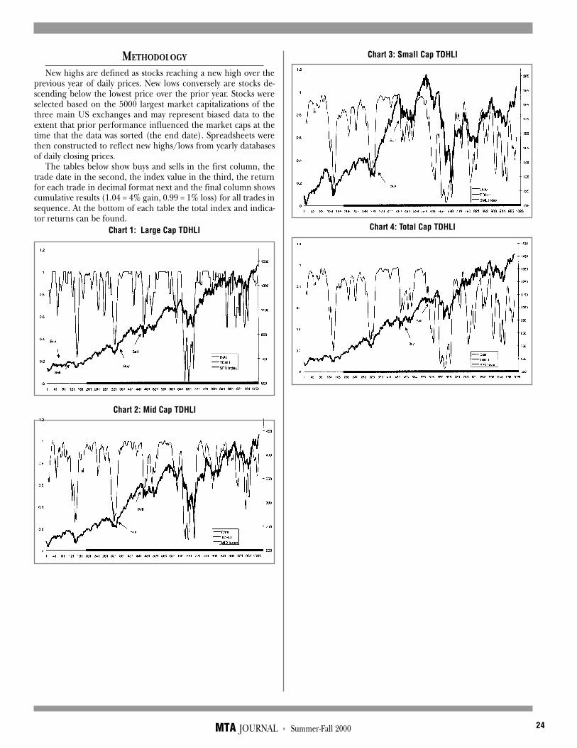
MTA JOURNAL • Summer-Fall 2000 24
METHODOLOGY
New highs are defined as stocks reaching a new high over theprevious year of daily prices. New lows conversely are stocks de-scending below the lowest price over the prior year. Stocks wereselected based on the 5000 largest market capitalizations of thethree main US exchanges and may represent biased data to theextent that prior performance influenced the market caps at thetime that the data was sorted (the end date). Spreadsheets werethen constructed to reflect new highs/lows from yearly databasesof daily closing prices.
The tables below show buys and sells in the first column, thetrade date in the second, the index value in the third, the returnfor each trade in decimal format next and the final column showscumulative results (1.04 = 4% gain, 0.99 = 1% loss) for all trades insequence. At the bottom of each table the total index and indica-tor returns can be found.
Chart 1: Large Cap TDHLI
Chart 3: Small Cap TDHLI
Chart 4: Total Cap TDHLI
Chart 2: Mid Cap TDHLI

MTA JOURNAL • Summer-Fall 2000 25
Table 3Mid Cap Rates of Return Mid Cap using Traditional Rules
Date MID Return Index Date MID Return Index
b 01/25/96 215.67 100 b 07/19/96 221.66 100
s 03/04/96 228.51 5.95% 105.9535 s 12/18/96 249.87 12.73% 112.7267
b 03/20/96 230.28 b 04/16/97 251.47
s 06/17/96 237.87 3.30% 109.4458 s 10/27/97 308.39 22.63% 138.2423
b 07/02/96 236.98 b 09/16/98 308.5
s 07/15/96 218.6 -7.76% 100.9572 s 02/12/99 367.09 18.99% 164.4971
b 07/19/96 221.66
s 09/03/96 231.21 4.31% 105.3069 Total 27.68%
b 09/16/96 238.76 MID 65.61%
s 12/16/96 247.16 3.52% 109.0117
b 01/02/97 252.11
s 03/13/97 263.14 4.38% 113.7811
b 04/08/97 255.84
s 04/10/97 253.76 -0.81% 112.856
b 04/16/97 251.47
s 10/24/97 329.48 31.02% 147.8658
b 11/06/97 325.13
s 12/19/97 320.26 -1.50% 145.651
b 01/05/98 333.39
s 05/26/98 363.22 8.95% 158.683
b 06/26/98 356.97
s 07/24/98 357.91 0.26% 159.1009
b 08/17/98 329.85
s 08/31/98 299.86 -9.09% 144.6354
b 09/08/98 291.65
s 10/07/98 289.31 -0.80% 143.475
b 10/16/98 305.41
s 02/08/99 367.23 20.24% 172.5167
b 03/10/99 364.25
s 03/29/99 363.05 -0.33% 171.9483
b 04/08/99 362.46
s 06/01/99 395.87 9.22% 187.7978
b 06/16/99 399.73
s 07/26/99 415.37 3.91% 195.1456
b 08/19/99 400.3
s 09/16/99 401.09 0.20% 195.5307
b 10/06/99 384.82
s 10/19/99 369.5 -3.98% 187.7465
b 10/29/99 391.2
s 12/15/99 411.75 5.25% 197.609
Total 97.61%
MID 90.92%
Table 2Large Cap Rates of Return Large Cap using Traditional Rules
Date SPX Return Index Date SPX Return Index
b 01/31/96 636.02 100.000 s 03/12/96 637.09 100.000
s 03/08/96 633.5 -0.40% 99.60379 b 07/31/96 639.95 -0.45% 99.55309
b 03/22/96 650.62 s 12/17/96 726.04 13.45% 112.9456
s 06/26/96 664.39 2.12% 101.7118 b 08/24/98 1088.14
b 07/05/96 657.44 s 02/12/99 1230.13 13.05% 127.6837
s 07/12/96 646.19 -1.71% 99.97137
b 07/25/96 631.17 Total 27.68%
s 09/05/96 649.44 2.89% 102.8652 SPX 93.09%
b 09/19/96 683
s 12/13/96 728.64 6.68% 109.7389
b 12/30/96 753.85
s 01/27/97 765.02 1.48% 111.3649
b 02/07/97 789.56
s 03/20/97 782.65 -0.88% 110.3903
b 04/21/97 760.37
s 08/21/97 925.05 21.66% 134.2985
b 08/29/97 899.47
s 10/23/97 950.69 5.69% 141.9461
b 11/10/97 921.13
s 12/15/97 963.39 4.59% 148.4583
b 01/06/98 966.58
s 04/28/98 1085.1 12.26% 166.6635
b 06/25/98 1129.3
s 07/27/98 1147.3 1.59% 169.3186
b 08/17/98 1083.7
s 09/01/98 994.24 -8.25% 155.3455
b 09/11/98 1009.1
s 10/07/98 970.68 -3.80% 149.4369
b 10/14/98 1005.5
s 02/12/99 1230.1 22.34% 182.8158
b 03/01/99 1236.2
s 05/25/99 1284.4 3.90% 189.9501
b 06/08/99 1317.3
s 08/31/99 1320.4 0.23% 190.3942
b 09/02/99 1319.1
s 09/24/99 1277.4 -3.17% 184.3682
b 10/07/99 1317.6
s 10/18/99 1254.1 -4.82% 175.4817
b 10/28/99 1342.4
s 12/31/99 1469.3 9.45% 192.0581
Total 92.06%
SPX 131.01%

MTA JOURNAL • Summer-Fall 2000 26
Table 4Small Cap Rates of Return Small Cap using Traditional Rules
Date SML Return Index Date SML Return Index
b 02/02/96 122.95 100 b 08/02/96 128.73 100
s 06/18/96 134.96 9.77% 109.7682 s 10/29/96 136.1 5.73% 105.7252
b 07/30/96 123.87 b 04/08/97 139.27
s 11/01/96 136.48 10.18% 120.9426 s 10/28/97 178.17 27.93% 135.2556
b 11/13/96 139.67 b 06/08/98 190.86
s 03/05/97 146.21 4.68% 126.6057 s 12/10/98 164.75 -13.68% 116.7524
b 04/16/97 137.27 b 03/04/99 161.45
s 10/27/97 174 26.76% 160.4822 s 05/24/99 177.79 10.12% 128.5687
b 12/03/97 179.37 b 08/16/99 179.48
s 01/16/98 176.1 -1.82% 157.5566 s 11/22/99 185.95 3.60% 133.2034b 02/04/98 183.33
s 05/06/98 200.67 9.46% 172.4588 Total 33.20%
b 06/25/98 188.79 SML 44.45%
s 07/24/98 183.18 -2.97% 167.3341
b 08/07/98 175.83
s 08/26/98 160.54 -8.70% 152.7829
b 09/08/98 152.35
s 10/07/98 133.73 -12.22% 134.11
b 10/15/98 139.4
s 12/14/98 161.26 15.68% 155.1405
b 12/29/98 171.51
s 01/27/99 172.17 0.38% 155.7375
b 03/01/99 160.47
s 03/24/99 155.23 -3.27% 150.652
b 04/07/99 158.75
s 05/25/99 175.68 10.66% 166.7184
b 06/28/99 182.07
s 07/28/99 183.64 0.86% 168.156
b 08/17/99 180.22
s 09/22/99 175.96 -2.36% 164.1812
b 10/07/99 176.07
s 10/18/99 168.96 -4.04% 157.5513
b 10/28/99 174.11
s 11/30/99 182.97 5.09% 165.5686
b 12/29/99 195.47
Total 65.57%
SML 58.98%
Table 5�Total Cap Rates of Return Total Cap using Traditional Rules
Date SPX Return Index Date SPX Return Index
b 02/01/96 638.46 100.0000 b 07/31/96 639.95 100
s 06/18/96 662.06 3.70% 103.6964 s 11/01/96 703.77 9.97% 109.9727
b 07/05/96 657.44 b 04/14/97 743.73
s 07/15/96 629.8 -4.20% 99.3368 s 10/27/97 876.99 17.92% 129.6773
b 07/30/96 635.26 s 06/24/98 1132.88
s 11/04/96 706.73 11.25% 110.5127 s 07/21/98 1165.07 2.84% 133.362
b 11/13/96 731.13 b 02/23/99 1271.18
s 12/18/96 731.54 0.06% 110.5747 s 05/25/99 1284.4 1.04% 134.749
b 01/02/97 737.01 b 10/05/99 1301.35
s 03/17/97 795.71 7.96% 119.3815 s 11/24/99 1417.08 8.89% 146.7323
b 04/21/97 760.37
s 10/27/97 876.99 15.34% 137.6914 Total 46.73%
b 11/11/97 923.78 SPX 121.44%
s 05/07/98 1095.14 18.55% 163.233
b 06/24/98 1132.88
s 07/24/98 1140.8 0.70% 164.3741
b 08/12/98 1084.22
s 08/26/98 1084.19 0.00% 164.3696
b 09/08/98 1023.46
s 10/07/98 970.68 -5.16% 155.893
b 10/15/98 1047.49
s 12/14/98 1141.2 8.95% 169.8394
b 12/29/98 1241.81
s 01/28/99 1265.37 1.90% 173.0617
b 02/24/99 1253.41
s 03/24/99 1268.59 1.21% 175.1576
b 04/07/99 1326.89
s 05/25/99 1284.4 -3.20% 169.5487
b 06/28/99 1331.35
s 07/27/99 1362.84 2.37% 173.559
b 08/17/99 1344.16
s 09/21/99 1307.58 -2.72% 168.8357
b 10/06/99 1325.4
s 10/19/99 1261.32 -4.83% 160.6729
b 10/28/99 1342.44
s 12/01/99 1397.72 4.12% 167.2892
b 12/29/99 1463.46
Total 67.29%
SPX 118.92%
Table 6Trades Detailed
Cumulative Loses Large Cap Mid Cap Small Cap Total Cap
Traditional Rules -0.45% 0% -13.68% 0%
Dynamic Rules -23.03% -24.26% -35.38% -20.11%
Largest Loss -8.25% -9.09% -12.22% -5.16%
Cumulative Loses Large Cap Mid Cap Small Cap Total Cap
Traditional Rules 28.13% 27.68% 46.88% 46.73%
Dynamic Rules 115.09% 121.87% 100.95% 87.40%
Largest Loss 22.34% 31.02% 26.76% 18.55%

MTA JOURNAL • Summer-Fall 2000 27
OBSERVATIONS
After evaluating the TDHLI performance characteristics basedon proprietary new high/low data, the first conclusion was that asmy previous study showed, the traditional buy/sell rules did notwork effectively. Another conclusion was that the TDHLI usingdynamic rules performed better than the traditional rules, but didnot perform as well in the current period than it did in the earlierstudy. The slippage between trades based on the TDHLI was par-tially responsible for a return deficit compared to the S&P 500 overthe evaluation period. In strongly trending markets, any tradingactivity tends to negatively impact overall performance. The S&P500 was interrupted in its upward march only by two corrections,one 22.5% and the other 13%. It is interesting to note that usingaggregate data, the TDHLI lost only 5.16% during the 22.5% Oc-tober 1998 decline in the S&P 500. Similarly during the pullbacklast Fall, the TDHLI fell 7.55% versus 13% in the S&P 500 In fact,the most significant slippage in relative performance occurredaround periods of high performance: by either starting late or fin-ishing prematurely during a significant market move, the TDHLIunderper-formed the averages.
Loss management was a significant issue for the TDHLI overeach of the subdivisions of the data. Relatively large losses wereincurred as the TDHLI moved to a sell, but the market reactedmore sharply. Given the significant bifurcation of the markets dur-ing the last four years, an increasing number of stocks are laggingthe performance of the averages. Put another way, fewer and fewerstocks are leading the way higher and the volatility of the averagesis increasing. This effect has been documented in the media. Thisstratification implies that the timing value of new highs/lows willbe diminished for the time being. Due to the magnitude of thedata management task, a more comprehensive study was not pos-sible using PC based computing.
Still, the predictive power of new high/low data remains formi-dable. In each case, the periods of time excluded by the TDHLIunderperformed substantially in each market cap segment andacross all the data. For large caps, the excluded returns were 12.37%vs. 92.06% for the TDHLI. For mid cap data, the excluded returnswere slightly negative compared to nearly triple digit positive re-turns for the TDHLI. The small cap segment mirrored this result,but the TDHLI provided a less robust performance, in line withthe mid cap index, MID. Only in the aggregate data did the ex-cluded returns amount to much, with a 37.02% gain versus 67.09%for the TDHLI and 118.92% for the S&P 500. In spite of the obvi-ous applicability of the Wall Street maxim that its the time in themarket, not the market timing that yields the best results, the riskas measured by standard deviation suggests that the TDHLI wasexposed to less risk over the period. Granted that the market vola-tility recently has been extraordinary, the TDHLI standard devia-tions for each market cap and for aggregate data remained in singledigits (8.3%, 9.5%, 9.6%, 6.9% for large, mid, small and total capgroups respectively) while the market indices ranged between 630%for Nasdaq and 23% for the small cap, SML index.
The dynamic TDHLI signaled trades more often than the tradi-tional rules, which is consistent with prior results. The number oftotal trades (and losing trades) for each segment were 20 (7) forlarge caps, 20 (7) for mid caps, 17 (7) for small caps and 18 (5) foraggregate data. The magnitude of losses averaged about 25% ofgains. Looking beyond the market's extraordinary performance,the TDHLI provided fairly respectable results.
Performance of the dynamic filter method for the TDHLI wasrespectable compared to the traditional rules, but less robust
against the averages. The large cap dynamic indicator returned92.06% vs. 27.68% for traditional rules and 131.03% for the SPX.The mid cap indicator was up 97.61% vs. traditional rules with64.50% and MID at 90.92%. The small cap results were 65.57% vs.traditional methods with 33.20% and SML at 58.98%. The aggre-gate return was 67.29% vs. traditional rules with 46.73% and SPXat 118.92%. The essential difference was that by tracking the rela-tive movements of the TDHLI and signaling reversals of interme-diate magnitude, significant moves in the market were captured bythe indicator. On the other hand, the TDHLI in the current pe-riod tended to prematurely exit the market while meaningful re-turns remained. One interpretation of this result is that a diver-gence between a few stocks with high returns and the majority ofstocks with much less robust results over the period has created adistortion in market returns that is not fully captured by the newhigh/low data.
CONCLUSION
The traditional TDHLI and, in the current period, the dynamicTDHLI as well, failed to keep pace with the market despite postingstrong results. The utilization of proprietary data made the TDHLIconsiderably more flexible and provided new and interesting di-mensions to the indicator. While it provided useful sell and buysignals under most conditions, the TDHLI even with the addedfunctionality of proprietary data did not perform well enough androbustly enough to be considered an effective indicator solely onits own. The ability to predict market direction, to provide reason-ably competitive performance particularly considering results frommy prior study and to track the market along the lines of marketcapitalization may prove over time to be a worthwhile addition tothe art of technical analysis as embodied by the TDHLI.
ATTRIBUTION
■ Joseph Redegeld, The Ten Day New High/New Low Index, 1986.■ A.W. Cohen, Three-Point Reversal Method of Point & Figure Stock
Market Trading, 8th Edition, 1984, Chartcraft, Inc., pg 91.■ 2Data was provided by Factset, Inc.
RICHARD T. WILLIAMS, CFA, CMTRichard Williams is a Senior Vice President and Fundamen-
tal/Technical analyst for Jefferies & Company. He specializesin enterprise software and e-commerce infrastructure stocks.During 1999, his stock and convertible (equity substitute) rec-ommendations returned in excess of 360%, making him thetop performing software analyst based on Bloomberg data.Prior to joining Jefferies in 1997, Mr. Williams was an institu-tional salesman at Kidder Peabody/Paine Webber from 1992-97 and a convertible and warrant sales trader from 1988-92.
Mr. Williams received his MBA in Finance from NYU's SternSchool of Business in 1991. He received a B.A. in Governmentand Computer Science from Dartmouth College. He is a Char-tered Financial Analyst and a Chartered Market Technician.Mr. Williams is a member of the Association for InvestmentManagement & Research and the Market Technicians Asso-ciation. He was recently voted runner-up for the Charles Dowaward, for contributions to the body of technical knowledge.He has published several articles in the MTA Journal, been afrequent Radio Wall Street guest and is regularly quoted inthe foreign/domestic press and magazines.
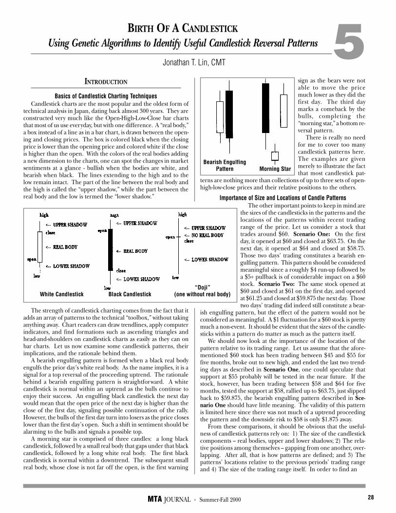
MTA JOURNAL • Summer-Fall 2000 28
White Candlestick Black Candlestick“Doji”
(one without real body)
Bearish EngulfingPattern Morning Star
INTRODUCTION
Basics of Candlestick Charting TechniquesCandlestick charts are the most popular and the oldest form of
technical analysis in Japan, dating back almost 300 years. They areconstructed very much like the Open-High-Low-Close bar chartsthat most of us use everyday, but with one difference. A “real body,”a box instead of a line as in a bar chart, is drawn between the open-ing and closing prices. The box is colored black when the closingprice is lower than the opening price and colored white if the closeis higher than the open. With the colors of the real bodies addinga new dimension to the charts, one can spot the changes in marketsentiments at a glance - bullish when the bodies are white, andbearish when black. The lines extending to the high and to thelow remain intact. The part of the line between the real body andthe high is called the “upper shadow,” while the part between thereal body and the low is termed the “lower shadow.”
The strength of candlestick charting comes from the fact that itadds an array of patterns to the technical “toolbox,” without takinganything away. Chart readers can draw trendlines, apply computerindicators, and find formations such as ascending triangles andhead-and-shoulders on candlestick charts as easily as they can onbar charts. Let us now examine some candlestick patterns, theirimplications, and the rationale behind them.
A bearish engulfing pattern is formed when a black real bodyengulfs the prior day’s white real body. As the name implies, it is asignal for a top reversal of the proceeding uptrend. The rationalebehind a bearish engulfing pattern is straightforward. A whitecandlestick is normal within an uptrend as the bulls continue toenjoy their success. An engulfing black candlestick the next daywould mean that the open price of the next day is higher than theclose of the first day, signaling possible continuation of the rally.However, the bulls of the first day turn into losers as the price closeslower than the first day’s open. Such a shift in sentiment should bealarming to the bulls and signals a possible top.
A morning star is comprised of three candles: a long blackcandlestick, followed by a small real body that gaps under that blackcandlestick, followed by a long white real body. The first blackcandlestick is normal within a downtrend. The subsequent smallreal body, whose close is not far off the open, is the first warning
sign as the bears were notable to move the pricemuch lower as they did thefirst day. The third daymarks a comeback by thebulls, completing the“morning star,” a bottom re-versal pattern.
There is really no needfor me to cover too manycandlestick patterns here.The examples are givenmerely to illustrate the factthat most candlestick pat-
terns are nothing more than collections of up to three sets of open-high-low-close prices and their relative positions to the others.
Importance of Size and Locations of Candle PatternsThe other important points to keep in mind are
the sizes of the candlesticks in the patterns and thelocations of the patterns within recent tradingrange of the price. Let us consider a stock thattrades around $60. Scenario One: On the firstday, it opened at $60 and closed at $63.75. On thenext day, it opened at $64 and closed at $58.75.Those two days’ trading constitutes a bearish en-gulfing pattern. This pattern should be consideredmeaningful since a roughly $4 run-up followed bya $5+ pullback is of considerable impact on a $60stock. Scenario Two: The same stock opened at$60 and closed at $61 on the first day, and openedat $61.25 and closed at $59.875 the next day. Thosetwo days’ trading did indeed still constitute a bear-
ish engulfing pattern, but the effect of the pattern would not beconsidered as meaningful. A $1 fluctuation for a $60 stock is prettymuch a non-event. It should be evident that the sizes of the candle-sticks within a pattern do matter as much as the pattern itself.
We should now look at the importance of the location of thepattern relative to its trading range. Let us assume that the afore-mentioned $60 stock has been trading between $45 and $55 forfive months, broke out to new high, and ended the last two trend-ing days as described in Scenario One, one could speculate thatsupport at $55 probably will be tested in the near future. If thestock, however, has been trading between $58 and $64 for fivemonths, tested the support at $58, rallied up to $63.75, just slippedback to $59.875, the bearish engulfing pattern described in Sce-nario One should have little meaning. The validity of this patternis limited here since there was not much of a uptrend proceedingthe pattern and the downside risk to $58 is only $1.875 away.
From these comparisons, it should be obvious that the useful-ness of candlestick patterns rely on: 1) The size of the candlestickcomponents – real bodies, upper and lower shadows; 2) The rela-tive positions among themselves – gapping from one another, over-lapping. After all, that is how patterns are defined; and 3) Thepatterns’ locations relative to the previous periods’ trading rangeand 4) The size of the trading range itself. In order to find an
BIRTH OF A CANDLESTICK
Using Genetic Algorithms to Identify Useful Candlestick Reversal Patterns
Jonathan T. Lin, CMT5

MTA JOURNAL • Summer-Fall 2000 29
effective candlestick pattern, these points should all be consid-ered integral parts of the pattern definition.
[Author’s Note: Although volume and open interest accompanyingthe candlestick patterns could be used as confirmation, the author has de-cided not to include either as part of the pattern definition for two reasons:1) A stock can rally or decline without increasing volume. Volume tends tobe more evident around structural breakouts and breakdowns, but not al-ways so around early reversal points. This is especially true for thinly-traded stocks where the price can move either way quickly without muchvolume. Depending on volume as confirmation is impractical at times. 2)The pattern the author plans to find should be rather universal just like theother candlestick patterns. Shooting stars are not unique to crude oil fu-tures; nor is the bearish engulfing pattern only designed for Microsoft stock.Since some market data, such as spot currencies and interest rates, do notcontain volume nor open interest information, a candlestick pattern withvolume or open interest as an integral part of it will not be universallyuseful.]
Basics of Genetic Algorithm – “Survival of the Fittest” “Survival of the Fittest.” Darwin’s theory of evolution remains
one of the scientific theories that has had the most profound im-pact on humankind to date. In his theory, Darwin proposed thatspecies evolve through natural selection, that is, species’ chance ofexistence and their ability to procreate depend on their ability toadapt to their natural habitat. Since only the organisms fit for theirnatural environment survive, only the genes they carry survive.During the reproductive process, the next generation of organ-isms are created from the genes drawn from the surviving, andhopefully superior, gene pool. The new generation of organismsshould, in theory, be even more adaptive to their environment. Assome of the offspring produced will certainly be more adaptive tothe environment than their peers and therefore survive, the natu-ral selection process repeats itself, and again only “superior” geneswill be left in the gene pool. As the process is repeated generationsafter generations, nature will preserve only the “fittest” genes anddispose of the “inferior” ones. It should be noted that during theprocess, the genes sometimes will experience certain degrees ofmutation that might create combinations of genes never seen inprevious generations. Mutation actually brings about a more di-versified pool of genes, perhaps creating even more adaptive or-ganisms than otherwise possible. At times in nature, an array ofspecies evolve from the same origin, with each of them as fit for itshabitat as the others in its own right.
So, what is “genetic algorithm?” In plain English, genetic algo-rithm is a computer program’s way of finding solutions to a prob-lem by the process of eliminating poor ones and improving on thebetter ones, mimicking what nature does. In constructing a ge-netic algorithm, one would start out by defining the problem to besolved in order to decide on the evaluation procedure, imitatingthe process of natural selection. Try a few possible solutions to aproblem. Rank them based on their performance after applyingthe evaluation process. Keep only the top few solutions and letthem reproduce, or mix elements of the top solutions to come upwith new ones. The new solutions are then, in turn, evaluated.After a few iterations, or generations, the best solutions will prevail
For a better explanation, we should now try a fun, practical ex-ercise. Let us consider the process of finding that perfect recipefor a margarita. We start out with six randomly mixed glasses; recordthe proportion between tequila and the lime juice and taste them.The evaluation process here is your friends’ reactions. They agreedthat two glasses were found okay, three of them so-so, and one whichyielded the response, “My dog is a better bartender than you.” You
then mix five more glasses using proportions somewhere betweenthose found in two okay glasses, and throw in one wildcard, a ran-domly mixed sample. Now let them try picking the two best onesagain. After you get your friends stone-drunk after repeating thisprocess 20 times, you will have yourself two nice glasses of margarita.Most importantly, those two glasses should be of similar propor-tion of lime juice and tequila; that is, the solution to this problemconverged.
Let us now review our margarita experiment. The goal was tofind the best tasting margaritas, and therefore the way to evaluatethem was to taste them and rate them. Assuming that you have anobjective way to total your friends’ opinions of the samples, theones that survived by this “somewhat natural selection” – the okayglasses – will get to “reproduce.” The wildcard thrown in repre-sents the mutated one. Just like mutations’ importance in natureas a way of injecting new genes into the gene pool and bringingabout a more diverse array of species, artificial mutations are veryimportant in opening up more possibilities in the range of solu-tions for the problem we intend to solve.
In a more involved problem with more variables, the procedureshould be repeated many more than 20 times for any half-way de-cent solutions to prevail. The more iterations the program per-form, the more optimal the solution should be. In fact, if the sur-viving solutions do not resemble each other at all, they are prob-ably far from optimal and require more time to evolve. What weare searching for here are “sharks.” Sharks, one of the fastest spe-cies in water, have been swimming in the ocean for millions of years.For generations, the faster ones survived by getting to their foodfaster in a feeding frenzy. Only the “fast” genes are left after allthese years. As sharks’ efficient hydrodynamic lines became “per-fect,” all of them started to “look alike.” (At least to most of us.)
End Note: To explain the concept of genetic algorithm in anacademic manner, I will turn to the principles set forth by JohnHolland, who pioneered genetic algorithms in 1975:1. Evolution operates on encodings of biological entities, rather than on
the entities themselves.2. Nature tends to make more descendants of chromosomes that are more
fit.3. Variation is introduced when reproduction occurs.4. Nature has no memory. [Author: Evolution has no intelligence
built in. Nature does not learn from previous results and fail-ures; it just selects and reproduces.]
Now the steps of the algorithm:1. Reproduction occurs.2. Possible modification of children occurs.3. The children undergo evaluation by the user-supplied evaluation func-
tion.4. Room is made for the children by discarding members of the population
of chromosomes. (Most likely the weakest population members.)
Definition of the Project’s Intent: Applying Genetic Algorithm toIdentify Useful Candlestick Reversal Patterns
Let me now define the problem I intend to solve in this study. Iintend to find one candlestick pattern that has good predictabilityin spotting near-term gains in future price by using the bond fu-tures contract as my testing environment. Since I have cited sharksas the marvelous products of natural selection, I would like to callthe organisms that should evolve through my study “candlesharks.”
The candlesharks will have genes that tell them when to signalpotential gains, or “eat” if one would parallel them to the real sharks.The first generation candlesharks should be pretty “dumb” and not

MTA JOURNAL • Summer-Fall 2000 30
really know when or when not to “eat” – maybe some are eating allthe time while some simply do not move at all. As some of themover ate or starved to death, the smarter ones knew how to “eatright,” correctly spotting potential for profit. As only the smartones survive, they begin to preserve only the smart genes. As thesesmarter ones mate and reproduce, some of the next generationmay contain, by chance, some even better combination of genes,resulting in even smarter candlesharks. As the process continues,the candlesharks should evolve to be pretty smart eaters. Once in awhile, some genes will mutate, creating candlesharks unlike theirparents. Whether the newly injected genes will be included in thegene pool will depend on the success of these mutated creatures inadapting to their environment.
One thing that should be pointed out is that the late genera-tion candlesharks will probably swim better in “bond futures pool”better than in a “spot gold pool” or “equity market pool” whichthey have never been in before. “Survival of the fittest” is more like“survival of the curve-fittest” here. It should be understood thatthe candlestick pattern found here has evolved within the “bond”environment and thus is best-fit for it. If thrown into the “spotgold pool,” these candlesharks might “die” like the dinosaurs didwhen the cold wind blew as the Ice Age hit them so unexpectedly,as one of the many theories goes. As in many cases in life, the finera design with one purpose in mind, whether natural or artificial,the less adaptive it will be when used for other purposes. For ex-ample, a 16-gauge wire stripper, while great with 16-gauge wires,will probably do a lousy job stripping 12-gauge wires even whencompared to a basic pair of scissors, which can strip any wire thoughslowly.
BUILDING A SUITABLE ENVIRONMENT FOR
EVOLUTION
Defining the GenesAs described in the previous sections, there are, but not limited
to, four major deciding factors of the significance of an occurrenceof a particular candlestick pattern. They include the size of therecent trading range, current position within that range, relativeposition of the candlesticks to each other, and the sizes of the thosecandlesticks. To successfully survive in the “bond futures pool,” itmust be in the genes of the candlesharks to be able to distinguishvariations in these environmental parameters. I have thereforedesigned a candleshark to possess the listed genes in Exhibit 1. Geneswithin Chromosome C-2, for example, tells the candleshark the rangeof position and size of the candlestick of two days ago should bewithin, combined with other chromosome’s parameters, beforegiving a bullish signal. Actually, think of all these genes as simplytandem series of on-off switches for a candleshark to decide to give abullish signal or not.
All the genes defined here come in pairs. The first, with suffix“-m”, tells the candleshark the minimum of the range in question.The second, with suffix “+”, signifies the width of the range. Hereis one example. If RB-m of C2 is -24 and RB+ of C2 is 16, thecandleshark will only give a bullish signal when the candlestick oftwo trading days ago has a black real body sized between 8 (-24 + 16= -8) ticks and 24 ticks, or the contract closed between _ to _ lowerthan it opened. Please keep in mind that C2 only contributes to apart of the decision-making process for the candleshark. Even if thereal body of two days ago fits the criteria, the other criteria have tobe met as well before the candleshark will actually give a bullish sig-nal.
The number of digits needed within each gene can be calcu-lated. The size of a real body for a bond contract can not be largerthan 96 ticks since the daily trading limit is set to three points. Aseven-bit binary number is capable of handing numbers up to 128and therefore needed for a gene like RB-m of C2. The 40-day trad-ing could be no larger than 96 ticks times 40, or 3840 ticks. (Be-sides the fact that it seems very unlikely that the bond contractwould go up, or down, 3 points day after day for 40 days.) A 12-bitnumber, capable of handing a decimal number up to 4096 is neededhere.
As the reader might have noticed after referencing Exhibit 1, anumber of trading ranges are used. As previously mentioned, thesize of the recent trading range and the candle pattern’s positionwithin the range are crucial elements that might make or breakthe pattern. How does one define “recent” though? It then seemedobvious to me that a multitude of day ranges is needed here, muchlike the popular practice of using a number of moving averages toaccess the crosscurrents of shorter and longer-term trends. I havechosen to include 5-day, 10-day, 20-day and 40-day trading ranges,which are more or less one, two, four, and eight trading weeks, inmy study. The advantage of using a multitude of day ranges couldbe demonstrated using two examples. Let us say a morning star, abullish candlestick reversal pattern, was found near when the priceis at the bottom of both the five-day trading range and the 40-daytrading range, as it would if it was just making a new reaction low.A morning star around this level is probably less useful since thatpattern is more indicative of a short-term bounce. While this morn-ing star, a one-day pattern, could be signaling a possible turn ofthe trend of the last five days, it is unconvincing that this one-daypattern could signal an end to the trend that lasted at least 40 days.
Let us now say that the same morning star was found near thebottom of the five-day trading range, but near the top of the 40-daytrading range, as the price of a stock would if it experienced a short-term pullback after breaking out of a longer-term trading range.This morning star now could be a signal for the investor to go longthe stock. The morning stars in both examples could be of thesame size, both found near the bottom of the five-day trading range,but would have significantly different implications just because theyappear at the different points of the 40-day trading range. It shouldbe clear now that the inclusion of multiple trading ranges in thedecision-making process could be very beneficial.
Since each gene is a binary number, a string of 0’s and 1’s, eachwill have a MSB (most significant bit, the leftmost digit, like 3 in39854) and LSB (least significant bit, the rightmost digit.) Sincethe MSB obviously has more impact on the candlesharks’ behavior,the common state of the more significant bits among the candlesharksare what we should closely examine after the program has let thecandlesharks breed for a while. The candlesharks’ main featuresshould be similar after a while. That is, if we do have a nice batchof candlesharks to harvest, they should all have the same sets of 0’sand 1’s among the more significant bits within each gene. The 0’sand 1’s among the trailing bits are less significant by comparison,much like the curvature of an athlete’s forehead should have lessto do with his speed than his torso structure. The trailing bits arein the genes and do make a difference, but are basically not signifi-cant enough for us to worry about.
When we are ready to harvest our candleshark catches as theperformance improvement from one generation to the next de-creased to a very small level, we could reverse-engineer the gene tofind the criteria that trigger their bullish signals. For instance, ifall eight candlesharks have “-00011” as the first five digits in RB-m ofC2 (that means RB-m is between -00011000 and -00011111, or -24

MTA JOURNAL • Summer-Fall 2000 31
and -31) and “00000” as the first five digits of RB+ of C2 (thatmeans RB+ is between 0000000 and 0000011, or 0 and 3), thesecandlesharks would only give bullish signals when the real body oftwo days ago is black, and between size of -21 and -31. (The mini-mum = -31 + 0 = -31; the maximum = -24 + 3 = -21)
Defining the Evaluation ProcessI have weighed several methods to evaluate the performance of
each of the organisms. First of all, a suitable method has to be ofshort-term nature since the pattern in question is basically formedin three days. It is very unlikely that, for instance, a morning starformed in three days that occurred twenty days ago has much in-fluence on current price. Secondly, the upward price movementthat comes after the pattern has to be greater than the downwardmovement, at least on the average. It should be realized that nomatter how useful a candlestick pattern, or any technical tool, maybe, there will be a time that it would not have predictive ability, oreven give a downright wrong signal. It then seems reasonable thatincluding total downward moves is essential in the evaluation pro-cess. That is, we would like to find a pattern that is not only rightand right enough most of the time, but one that will not take any-one to the cleaners when it is wrong.
What I have decided on is the average of the maximum poten-tial gain less the maximum potential loss. First, we find the maxi-mum potential gain by totaling all the differences between the high-est of the high prices reached by the contract within the next fivetrading days from the closing price when the pattern gave the sig-nal. We then find the maximum potential loss by totaling all thedifferences between the lowest of the low prices reached by thecontract within the next five trading days from the closing pricewhen the pattern gave the signal. The maximum loss is subtractedfrom the maximum gain, and is then divided by the number ofsignals generated. This ratio is the average of the maximum po-tential gain less the maximum potential loss I am looking for.
Defining the Reproductive ProcessWe desire enough permutations of the parents’ genes to create
diversity among the offspring. Yet, too many offspring in each gen-eration would greatly increase the processing time needed to evalu-ate the performance of all the offspring. After a fair amount ofcontemplating, I believe that eight offspring from two parents isadequate. A trial run shows that the evaluation of eight organismswith 1,500 days worth of data requires roughly four minutes of pro-cessing time on my personal computer. That equals 1,080 genera-tions after three straight days of processing. Since a large numberof generations might be required for the effective evolution, eightorganisms per generation would have to do. Besides, allowing onlytwo out of eight offspring to survive is a stringent enough elimina-tion process. Many large mammals have fewer offspring in theirlife times.
The second crucial element of the reproduction is the intro-duction of mutation. Under the principles set forth by John Hol-land, mutations come in two modes: binary mutation, the replace-ment of bits on a chromosome with randomly generated bits, andone-point crossover, the swapping of genetic material on the childrenat a randomly selected point. I have favored a higher level of mu-tation since it would introduce more diverse gene sequences intothe gene pool more quickly. Both the binary mutation level andone-point crossover level have been set to 0.1, or 10% of the time.
EVALUATION OF RESULTS
Preliminary Results and ModificationsAs some people might have suspected, what I thought was a won-
derful study had a pretty rocky start. The final version of the genedefinition, as the readers know it, is actually the third revision. Alarge number of genes slows down the processing time dramati-cally. Having too many trading ranges defined also proved to be awaste of time.
Choosing the right gene pool to start with, much to my sur-prise, was in fact quite tricky. I first wrote a small routine using theVisual Basic Macro in Excel to randomly generate eight candlesharks.These candlesharks did indeed reproduce and the evolution pro-gram, also written in Visual Basic, performed its duty and evalu-ated each one of them. After testing the programs and becomingconvinced of their ability to perform their functions, I let the pro-gram run overnight, evolving 50 generations. What I found thenext morning were eight candlesharks that did absolutely nothing.None of them gave any signal. As they all performed equally poorly,the two selected to reproduce were basically chosen arbitrarily. WhatI had come up with were the equivalents of the species that wouldhave been extinct in nature.
The next logical step then was to use two organisms that wouldgive me signals all the time and to write a small routine to generatesix offspring from them. The eight of them would then be mystarting point. This proved to be much more effective. Since thefirst batch of candlesharks did indeed provide me more signals thanI needed, their offspring could only give an equal amount or lesssignals. As some of the children became more selective, their per-formance did improve. After viewing the printed results of thefirst seven or so generations, I was glad to see the gradual, yet steadyimprovement in the ability to find bullish patterns. I again let themgrow overnight.
What I found the next morning was a collection of candlesharksthat gave either one or two signals. Each of the signals was wonder-ful, pointing to large gains without much risk. As it turned out, afew of them were simply pointing to the same date. Thesecandlesharks basically curve-fitted themselves just to pick up the dayfollowed by the best five-day gain in the data series. They wereagain useless.
It then occurred to me that I had to set a minimum number ofsignals per organism that the candlesharks would have to meet be-fore the program would consider evaluating them as the breedingones. Since I was using 1,500 days, or roughly six years, worth ofdata, the minimum of 20 signals, or a little over three a year, shouldsuffice.
I am glad to report that things started to look up afterward. Ihave also decided that running the program with smaller iterationcould be beneficial. I began running only five generations eachtime so that I could observe the progress and make any necessaryadjustment. It was not until that most things had been fine-tunedthat I began my overnight number-crunching again.
Finding Useful Gene SequencesI first wrote the program with the intention to let the candlesharks
evolve and hoped to see them converge into a batch of similarly-shaped creatures. In other words, I was looking for a group ofconsistent performers. It so happened that in the evolution pro-gram, I had coded a line to print out the gene pool with the evalu-ation results after every generation. This feature was first put inplace as a way to monitor the time needed for each generation,
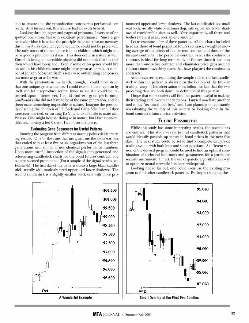
MTA JOURNAL • Summer-Fall 2000 32
A Wonderful Example Small Overlap of the First Two Candles
and to ensure that the reproduction process was performed cor-rectly. As it turned out, this feature had an extra benefit.
Looking through pages and pages of printouts, I every so oftenspotted one candleshark with excellent performance. Since a ge-netic algorithm is based on the principle that nature has no memory,this candleshark’s excellent gene sequence could not be preserved.The only traces of the sequence is in its children which might notbe as good a predictor as it was. This does occur in nature as well.Einstein’s being an incredible physicist did not imply that his chil-dren would have been, too. Even if some of his genes would liveon within his children, none might be as great as he was. A num-ber of Johann Sebastian Bach’s sons were outstanding composers,but none as great as he was.
With the printouts in my hands, though, I could reconstructthat one unique gene sequence. I could examine the organism byitself and let it reproduce several times to see if it could be im-proved upon. Better yet, I could find two great performingcandlesharks who did not have to be of the same generation, and letthem mate, something impossible in nature. Imagine the possibil-ity of seeing the children of J.S. Bach and Clara Schumann if theywere ever married, or turning Da Vinci into a female to mate withPicasso. One might hesitate doing so in nature, but I face no moraldilemma moving a few 0’s and 1’s all over the place.
Evaluating Gene Sequences for Useful PatternsRunning the program from different starting points yielded vary-
ing results. One of the runs that intrigued me the most was onethat ended with at least five or six organisms out of the last threegenerations with similar if not identical performance numbers.Upon more careful inspection of the signals they generated andreferencing candlestick charts for the bond futures contract, onepattern seemed prominent. (For a sample of the signal results, seeExhibit 6.) The first day of the pattern shows a large black candle-stick, usually with modestly sized upper and lower shadows. Thesecond candlestick is a slightly smaller black one with more pro-
nounced upper and lower shadows. The last candlestick is a smallreal body, usually white or at times doji, with upper and lower shad-ows of considerable sizes as well. Very importantly, all three realbodies rarely, if at all, overlap one another.
Let us examine a few of these patterns. All the charts includedhere are those of bond perpetual futures contract, a weighted mov-ing average of the prices of the current contract and those of theforward contracts. The perpetual contract, versus the continuouscontract, is ideal for long-term study of futures since it includesmore than one active contract and eliminates price gaps aroundcontract month switching dates that have plagued the continuouscontracts.
As one can see by examining the sample charts, the last candle-stick within the pattern is always near the bottom of the five-daytrading range. This observation does follow the fact that the twopreceding days are both down, by definition of this pattern.
I hope that some readers will find this pattern useful in makingtheir trading and investment decisions. I myself now have anothertool in my “technical tool belt,” and I am planning on constantlyre-evaluating the validity of this pattern by looking for it in thebond contract’s future price activities.
FUTURE POSSIBILITIES
While this study has some interesting results, the possibilitiesare endless. This study was set to find candlestick patterns thatwould identify possible up moves in bond prices in the next fivedays. The next study could be set to find a complete entry/exittrading system with both long and short positions. A different ver-sion of the devised program could be used to find an optimal com-bination of technical indicators and parameters for a particularsecurity instrument. In fact, the use of genetic algorithms as a wayto optimize neural networks has been widespread.
Looking not so far out, one could even use the existing pro-gram to find other candlestick patterns. By simply changing the

MTA JOURNAL • Summer-Fall 2000 33
Small Overlap of the First Two Candles
Less Successful Example, Perhaps Due to the LargerSecond Black Candle. Developed Only into a
Consolidation.
Slightly Different Example that Developed into a“Rising Three”
Overlapping of Real Bodies Again Led to a Less TimelyPattern.

MTA JOURNAL • Summer-Fall 2000 34
gene pool one starts with, very different organisms from theone we found might evolve. Much like different species in nature,of which each excels in its habitat and its own way, different candle-stick patterns can be found to be effective under different situa-tions. Change the gene pool a little and let the computer go at it.One day, your machine might find something to surprise you.
As the computers become faster and faster, one day I should beable to include a large number of organisms. Using a multitude ofselection/evaluation criteria, several species might evolve at thesame time, just like an ecosystem in nature. I might be able to find,after numerous iterations, one pattern particularly good for a five-day forecast while another one is found to have an excellent one-day forecasting ability. The possibilities are endless.
EXHIBITS AND BIBLIOGRAPHY
Exhibit 1Definition of Genes and Chromosomes
Chrom Gene
Name Name Description Format
C2 RB-m Minimum of real body size 2 days ago. 7-bit binary with sign-bit
RB+ Dev. from min. of real body size 2 days ago. 8-bit binary
US-m Minimum of upper shadow size 2 days ago. 7-bit binary
US+ Dev. from min. of upper shadow size 2 days ago. 7-bit binary
LS-m Minimum of lower shadow size 2 days ago. 7-bit binary
LS+ Dev. from min. of lower shadow size 2 days ago. 7-bit binary
C1 RB-m Minimum of real body size 1 day ago. 7-bit binary with sign-bit
RB+ Dev. from min. of real body size 1 day ago. 8-bit binary
US-m Minimum of upper shadow size 1 day ago. 7-bit binary
US+ Dev. from min. of upper shadow size 1 day ago. 7-bit binary
LS-m Minimum of lower shadow size 1 day ago. 7-bit binary
LS+ Dev. from min. of lower shadow size 1 day ago. 7-bit binary
CH-m Change of closing level from 2 days ago 7-bit binary with sign-bit
CH+ Change of closing level from 2 days ago 8-bit binary
C0 RB-m Minimum of current real body size. 7-bit binary with sign-bit
RB+ Dev. from min. of current real body size. 8-bit binary
US-m Minimum of current upper shadow size. 7-bit binary
US+ Dev. from min. of current upper shadow size. 7-bit binary
LS-m Minimum of current lower shadow size. 7-bit binary
LS+ Dev. from min. of current lower shadow size. 7-bit binary
CH-m Change of closing level from 1 day ago 7-bit binary with sign-bit
CH+ Change of closing level from 1 day ago 8-bit binary
R5D TR-m Minimum of 5-day trading range. 9-bit binary
TR+ Dev. from min. of 5-day trading range. 9-bit binary
RP-m Minimum of position within trading range. 9-bit binary
RP+ Dev. from min. of position within trading range. 9-bit binary
R10D TR-m Minimum of 10-day trading range. 10-bit binary
TR+ Dev. from min. of 10-day trading range. 10-bit binary
RP-m Minimum of position within trading range. 10-bit binary
RP+ Dev. from min. of position within trading range. 10-bit binary
R20D TR-m Minimum of 20-day trading range. 11-bit binary
TR+ Dev. from min. of 20-day trading range. 11-bit binary
RP-m Minimum of position within trading range. 11-bit binary
RP+ Dev. from min. of position within trading range. 11-bit binary
R40D TR-m Minimum of 40-day trading range. 12-bit binary
TR+ Dev. from min. of 40-day trading range. 12-bit binary
RP-m Minimum of position within trading range. 12-bit binary
RP+ Dev. from min. of position within trading range. 12-bit binary
Note: All the numbers in the genes are in ticks. A tick = 1/32move in bond futures. Bond futures has a limit of daily movementof no more than 3 points, or 96 ticks.

MTA JOURNAL • Summer-Fall 2000 35
Exhibit 2Test Bed: Sample Bond Futures Data Spreadsheet
Exhibit 3Gene Pool: Sample of Binary Bits
Exhibit 4Gene Pool: Sample of Gene in Decimals for Printing & Reading Purpose

MTA JOURNAL • Summer-Fall 2000 36
Exhibit 5Excel Macro – Visual Basic Program:
EVOLUTIONConst pop = 8, num_gene = 38, mutation_level = 0.1, crossover_level
= 0.1Const TB_sheet = “Test Bed”, GP_sheet = “Gene Pool”, SR_sheet =
“Signal Results”, GPD_sheet = “GP in Dec.”Const GP_row1 = 5, GP_col1 = 6Const SR_row1 = 4, SR_col1 = 1Const TB_row1 = 43, TB_col1 = 7Const generation_rep = 5, TB_sample_size = 1500, days_per_signal
= 5, min_num_signal = 20Dim gene_signed(num_gene), gene(pop, num_gene),
top_genes(2, num_gene) As StringDim gene_len(num_gene), limits(num_gene / 2, 2) As Integer
Sub EVOLUTION() Set GP = Worksheets(GP_sheet) Set GPD = Worksheets(GPD_sheet) Set SR = Worksheets(SR_sheet) Set TB = Worksheets(TB_sheet) For j = 1 To num_gene gene_len(j) = GP.Cells(3, GP_col1 + j - 1).Value gene_signed(j) = GP.Cells(4, GP_col1 + j - 1).Value Next j
gen_num = GP.Cells(1, 2).ValueFor generation = gen_num To gen_num + generation_rep - 1 SR_rowcount = SR_row1
SR.Select ‘Clear enough area for new Signal Results coming in
Rows(SR_row1 & “:” & pop * (Int(TB_sample_size /days_per_signal) +
2)).Select Selection.ClearContents GPD.Select GPD.Cells(1, 2).Value = GP.Cells(1, 2).Value For org = 1 To pop ‘ Evaluation each organism within popula-
tion utimate_gain = 0 utimate_loss = 0 total_gain = 0 total_loss = 0 num_signal = 0 GPD.Cells(GP_row1 + org - 1, 1).Value = GP.Cells(GP_row1 +
org - 1,1).Value For i = 1 To num_gene ‘ Convert binary gene bits to number
limits gene(org, i) = GP.Cells(GP_row1 + org - 1, GP_col1 + i - 1).Value If gene_signed(i) = “(signed)” Then If Left(GP.Cells(GP_row1 + org - 1, GP_col1 + i - 1).Value,
1) =“+” Then mult = 1 Else mult = -1 shift = 1 Else mult = 1 shift = 0 End If num = 0 For n = shift + gene_len(i) To shift + 1 Step -1 If Mid(gene(org, i), n, 1) = “1” Then num = num + 2 ^ (gene_len(i) - n + shift) End If Next n pointer = Int((i + 1) / 2) If i - (pointer - 1) * 2 = 1 Then limits(pointer, 1) = mult * num Else limits(pointer, 2) = limits(pointer, 1) + mult * num End If Next i For i = 1 To num_gene / 2 GPD.Cells(GP_row1 + org - 1, GP_col1 + (i - 1) * 2).Value =
limits(i, 1) GPD.Cells(GP_row1 + org - 1, GP_col1 + (i - 1) * 2 + 1).Value
= limits(i, 2) Next i
‘Start looking for signals signal = “NO” For i = 1 To TB_sample_size row_num = TB_row1 + i - 1 curr_date = TB.Cells(row_num, 2).Value
curr_close = TB.Cells(row_num, 6).Value If signal = “NO” Then signal = “YES” For j = 1 To num_gene / 2 If TB.Cells(row_num, TB_col1 + j - 1).Value < limits(j,
1) Or TB.Cells(row_num, TB_col1 + j - 1).Value > limits(j, 2)Then
signal = “NO” End If Next j If signal = “YES” Then SR_rowcount = SR_rowcount + 1 SR.Cells(SR_rowcount, 1).Value =
Application.Text(generation, “0000”) & “x” &Application.Text(org, “00”)
SR.Cells(SR_rowcount, 2).Value = curr_date SR.Cells(SR_rowcount, 3).Value = curr_close signal_row = row_num signal_price = curr_close num_signal = num_signal + 1 max_gain = 0 max_loss = 0 End If Else curr_high = TB.Cells(row_num, 4).Value curr_low = TB.Cells(row_num, 5).Value If curr_high - signal_price > max_gain Then max_gain = curr_high - signal_price high_date = curr_date high_price = curr_high End If If signal_price - curr_low > max_loss Then max_loss = signal_price - curr_low low_date = curr_date low_price = curr_low End If If row_num - signal_row >= days_per_signal Or i =
TB_sample_sizeThen
signal = “NO” SR.Cells(SR_rowcount, 4).Value = high_date SR.Cells(SR_rowcount, 5).Value = high_price SR.Cells(SR_rowcount, 6).Value = low_date SR.Cells(SR_rowcount, 7).Value = low_price total_gain = total_gain + max_gain total_loss = total_loss + max_lossIf max_gain > utimate_gain Then utimate_gain = max_gain If max_loss > utimate_loss Then utimate_loss = max_loss SR.Cells(SR_rowcount, 8).Value = num_signal SR.Cells(SR_rowcount, 9).Value = max_gain SR.Cells(SR_rowcount, 11).Value = max_loss End If End If Next i ‘ Signal summary for each organism SR_rowcount = SR_rowcount + 1 SR.Cells(SR_rowcount, 1).Value = Application.Text(generation,
“0000”) & “x” & Application.Text(org, “00”) SR.Cells(SR_rowcount, 2).Value = “Summary:” SR.Cells(SR_rowcount, 8).Value = num_signal SR.Cells(SR_rowcount, 9).Value = total_gain SR.Cells(SR_rowcount, 10).Value = utimate_gain SR.Cells(SR_rowcount, 11).Value = total_loss SR.Cells(SR_rowcount, 12).Value = utimate_loss SR.Cells(SR_rowcount, 13).Value = total_gain - total_loss GP.Cells(GP_row1 + org - 1, 2).Value = num_signal GP.Cells(GP_row1 + org - 1, 3).Value = total_gain GP.Cells(GP_row1 + org - 1, 4).Value = total_loss GPD.Cells(GP_row1 + org - 1, 2).Value = num_signal GPD.Cells(GP_row1 + org - 1, 3).Value = total_gain GPD.Cells(GP_row1 + org - 1, 4).Value = total_loss If num_signal > min_num_signal Then GP.Cells(GP_row1 + org - 1, 5).Value = (total_gain - total_loss)
/ num_signal GPD.Cells(GP_row1 + org - 1, 5).Value = (total_gain - total_loss)
/ num_signal Else GP.Cells(GP_row1 + org - 1, 5).Value = 0 GPD.Cells(GP_row1 + org - 1, 5).Value = 0 End If Next org
‘SORTING RESULTS TO FIND THE 2 FITTEST ORGANISMS GP.Select range(Cells(GP_row1, 1), Cells(GP_row1 + pop - 1, GP_col1 +
num_gene -1)).Select Selection.Sort Key1:=range(“E” + Trim(Str(GP_row1))),
Order1:=xlDescending, Header:= _ xlGuess, OrderCustom:=1, MatchCase:=False, Orientation:=
_ xlTopToBottom GPD.Select range(Cells(GP_row1, 1), Cells(GP_row1 + pop - 1, GP_col1 +
num_gene -1)).Select Selection.Sort Key1:=range(“E” + Trim(Str(GP_row1))),
Order1:=xlDescending, Header:= _ xlGuess, OrderCustom:=1, MatchCase:=False, Orientation:=
_ xlTopToBottom GPD.PrintOut Copies:=1 For org = 1 To 2 For i = 1 To num_gene top_genes(org, i) = GP.Cells(GP_row1 + org - 1, GP_col1 + i -
1).Value Next Next
‘MIXING GENES FOR THE NEXT GENERATION GP.Cells(1, 2).Value = generation + 1 For org = 1 To pop GP.Cells(GP_row1 + org - 1, 1).Value = Application.Text(generation
+ 1, “0000”) & “x” & Application.Text(org, “00”) For i = 1 To num_gene - 1 Step 2 Randomize which_parent = Int(Rnd * 2) + 1 gene_string1 = top_genes(which_parent, i) gene_string2 = top_genes(which_parent, i + 1) If Rnd < mutation_level Then gene_mutate = Int(Rnd * (gene_len(i) + gene_len(i + 1))) + 1 If gene_mutate <= gene_len(i) Then If gene_signed(i) = “(signed)” Then shift = 1 Else shift = 0 gene_bit = Mid(gene_string1, gene_mutate + shift, 1) If gene_bit = “0” Then gene_bit = “1” Else gene_bit = “0” End If gene_string1 = Left(gene_string1, gene_mutate - 1 + shift) &
gene_bit & Right(gene_string1, gene_len(i) - gene_mutate) Else gene_mutate = gene_mutate - gene_len(i) gene_bit = Mid(gene_string2, gene_mutate, 1) If gene_bit = “0” Then gene_bit = “1” Else gene_bit = “0” End If gene_string2 = Left(gene_string2, gene_mutate - 1) &
gene_bit & Right(gene_string2, gene_len(i + 1) - gene_mutate) End If End If GP.Cells(GP_row1 + org - 1, GP_col1 + i - 1).Value = “‘“ &
gene_string1 GP.Cells(GP_row1 + org - 1, GP_col1 + i).Value = “‘“ &
gene_string2 Next Next crossover = Rnd If crossover < crossover_level Then Do child1 = Int(Rnd * pop) + 1 child2 = Int(Rnd * pop) + 1 Loop While child1 = child2 XO_point = Int(Rnd * num_gene / 2) * 2 + 1 For j = 1 To XO_point new_gene = GP.Cells(GP_row1 + child1 - 1, GP_col1 + j -
1).Value GP.Cells(GP_row1 + child1 - 1, GP_col1 + j - 1).Value =
GP.Cells(GP_row1 + child2 - 1, GP_col1 + j - 1).Value GP.Cells(GP_row1 + child2 - 1, GP_col1 + j - 1).Value =
new_gene Next End If Next generationEnd Sub

MTA JOURNAL • Summer-Fall 2000 37
BIBLIOGRAPHY
■ Nison, Steve. Japanese Candlestick Charting Techniques: A Contem-porary Guide to the Ancient Investment Technique of the Far East. NewYork, N.Y.: New York Institute of Finance, 1991.
■ Deboeck, J. Guido, Editor. Trading on the Edge: Neural, Geneticand Fuzzy Systems for Chaotic Financial Markets. New York, N.Y.:John Wiley & Sons, Inc., 1994. Chapter 8 by Laurence Davis.Genetic Algorithm and Financial Applications.
■ Note: All gene definition as described in Exhibit V-1 and theExcel Macro program Evolution written in Visual Basic are oforiginal work, and therefore no further reference is given. Theauthor drew on the knowledge and experience as an electricalengineering and computer science major during undergradu-ate years and seven years as an programmer/analyst to developthe program.
JONATHAN T. LIN, CMTJonathan Lin has been with Salomon Smith Barney since
1994. In his capacity as a technical research analyst there, hecontributes to the weekly publications Market Interpretation,and Global Technical Market Overview. Prior to Salomon, hewas a technology specialist at Price Waterhouse for one year,and spent six years at Merrill Lynch as a senior programmer/analyst.
Jonathan has an MBA in management information systemsfrom Pace University, Lubin Graduate School of Business, anda BE in electrical engineering & computer science from StevensInstitute of Technology.
Exhibit 6Sample of Signal Results