Journal of Statistical Software · PDF fileJSS Journal of Statistical Software ... Estimation...
42
JSS Journal of Statistical Software MMMMMM YYYY, Volume VV, Issue II. doi: 10.18637/jss.v000.i00 stm: R Package for Structural Topic Models Margaret E. Roberts UCSD Brandon M. Stewart Princeton Dustin Tingley Harvard Abstract This vignette demonstrates how to use the Structural Topic Model stm R package. The Structural Topic Model allows researchers to flexibly estimate a topic model that includes document-level meta-data. Estimation is accomplished through a fast variational approximation. The stm package provides many useful features, including rich ways to explore topics, estimate uncertainty, and visualize quantities of interest. Keywords : structural topic model, text analysis, LDA, stm, R. 1. Introduction Text data is ubiquitious in social science research: traditional media, social media, survey data, and numerous other sources contribute to the massive quantity of text in the mod- ern information age. The mounting availability of, and interest in, text data has been the development of a variety of statistical approaches for analyzing this data. We focus on the Structural Topic Model (STM), and its implementation in the stm R package, which provides tools for machine-assisted reading of text corpora. 1 Building off of the tradition of proba- bilistic topic models, such as the Latent Dirichlet Allocation (LDA) (Blei et al. 2003), the Correlated Topic Model (CTM) (Blei and Lafferty 2007), and other topic models that have extended these (Mimno and McCallum 2008; Socher et al. 2009; Eisenstein et al. 2010; Rosen- 1 We thank Antonio Coppola, Jetson Leder-Luis, Christopher Lucas, and Alex Storer for various assistance in the construction of this package. We also thank the many package users who have written in with bug reports and feature requests. We extend particular gratitude to users on Github who have contributed code via pull requests including Ken Benoit, Patrick Perry, Chris Baker, Jeffrey Arnold, Thomas Leeper, Vincent Arel-Bundock, Santiago Castro, Rose Hartman and Github user sw1. We gratefully acknowledge grant support from the Spencer Foundation’s New Civics initiative, the Hewlett Foundation and The Eunice Kennedy Shriver National Institute of Child Health & Human Development of the National Institutes of Health under Award Number P2CHD047879. The content is solely the responsibility of the authors and does not necessarily represent the official views of any of the funding institutions. Additional details and development version at structuraltopicmodel.com
Transcript of Journal of Statistical Software · PDF fileJSS Journal of Statistical Software ... Estimation...

JSS Journal of Statistical SoftwareMMMMMM YYYY, Volume VV, Issue II. doi: 10.18637/jss.v000.i00
stm: R Package for Structural Topic Models
Margaret E. Roberts
UCSDBrandon M. Stewart
PrincetonDustin Tingley
Harvard
Abstract
This vignette demonstrates how to use the Structural Topic Model stm R package.The Structural Topic Model allows researchers to flexibly estimate a topic model thatincludes document-level meta-data. Estimation is accomplished through a fast variationalapproximation. The stm package provides many useful features, including rich ways toexplore topics, estimate uncertainty, and visualize quantities of interest.
Keywords: structural topic model, text analysis, LDA, stm, R.
1. Introduction
Text data is ubiquitious in social science research: traditional media, social media, surveydata, and numerous other sources contribute to the massive quantity of text in the mod-ern information age. The mounting availability of, and interest in, text data has been thedevelopment of a variety of statistical approaches for analyzing this data. We focus on theStructural Topic Model (STM), and its implementation in the stm R package, which providestools for machine-assisted reading of text corpora.1 Building off of the tradition of proba-bilistic topic models, such as the Latent Dirichlet Allocation (LDA) (Blei et al. 2003), theCorrelated Topic Model (CTM) (Blei and Lafferty 2007), and other topic models that haveextended these (Mimno and McCallum 2008; Socher et al. 2009; Eisenstein et al. 2010; Rosen-
1We thank Antonio Coppola, Jetson Leder-Luis, Christopher Lucas, and Alex Storer for various assistancein the construction of this package. We also thank the many package users who have written in with bugreports and feature requests. We extend particular gratitude to users on Github who have contributed codevia pull requests including Ken Benoit, Patrick Perry, Chris Baker, Jeffrey Arnold, Thomas Leeper, VincentArel-Bundock, Santiago Castro, Rose Hartman and Github user sw1. We gratefully acknowledge grant supportfrom the Spencer Foundation’s New Civics initiative, the Hewlett Foundation and The Eunice Kennedy ShriverNational Institute of Child Health & Human Development of the National Institutes of Health under AwardNumber P2CHD047879. The content is solely the responsibility of the authors and does not necessarilyrepresent the official views of any of the funding institutions. Additional details and development version atstructuraltopicmodel.com

2 Structural Topic Models
Zvi et al. 2010; Quinn et al. 2010; Ahmed and Xing 2010; Grimmer 2010; Eisenstein et al.2011; Gerrish and Blei 2012; Foulds et al. 2015; Paul and Dredze 2015), the Structural TopicModel’s key innovation is that it permits users to incorporate arbitrary metadata, defined asinformation about each document, into the topic model. With the STM, users can model theframing of international newspapers (Roberts et al. 2016b), open-ended survey responses inthe American National Election Study (Roberts et al. 2014), online class forums (Reich et al.2015), Twitter feeds and religious statements (Lucas et al. 2015), lobbying reports (Milnerand Tingley 2015) and much more.2
The goal of the Structural Topic Model is to allow researchers to discover topics and estimatetheir relationship to document metadata. Outputs of the model can be used to conducthypothesis testing about these relationships. This of course mirrors the type of analysis thatsocial scientists perform with other types of data, where the goal is to discover relationshipsbetween variables and test hypotheses. Thus the methods implemented in this paper helpto build a bridge between statistical techniques and research goals. The stm package alsoprovides tools to facilitate the work flow associated with analyzing textual data. The designof the package is such that users have a broad array of options to process raw text data,explore and analyze the data, and present findings using a variety of plotting tools.
The outline of this paper is as follows. In Section 2 we introduce the technical aspects of theSTM, including the data generating process and an overview of estimation. In Section 3 weprovide examples of how to use the model and the package stm, including implementing themodel and plots to visualize model output. Sections 4 and 5 cover settings to control detailsof estimation. Section 6 demonstrates the superior performance of our implementation overrelated alternatives. Section 7 concludes and the Appendix discusses several more advancedfeatures.
2. The Structural Topic Model
We begin by providing a technical overview of the STM model. Like other topic models, theSTM is a generative model of word counts. That means we define a data generating processfor each document and then use the data to find the most likely values for the parameterswithin the model. Figure 1 provides a graphical representation of the model. The generativemodel begins at the top, with document (D1, D2...), topic (T1, T2...), and word (w1, w2...)distributions generating documents that have metadata associated with them (Xd, where d
indexes the documents). Within this framework (which is the same as other topic modelslike LDA), a topic is defined as a mixture over words where each word has a probabilityof belonging to a topic. And a document is a mixture over topics, meaning that a singledocument can be composed of multiple topics. As such, the sum of the topic proportionsacross all topics for a document is one, and the sum word probabilities for a given topic isone.
Figure 1 and the statement below of the document generative process highlight the case wheretopical prevalence and topical content can be a function of document metadata. Topicalprevalence refers to how much of a document is associated with a topic (described on theleft hand side) and topical content refers to the words used within a topic (described on
2A fast growing range of other papers also utilize the model in a variety of ways. We maintain a list ofpapers using the software that we are aware of on our website structuraltopicmodel.com.

Journal of Statistical Software 3
the right hand side). Hence metadata that explain topical prevalence are referred to astopical prevalence covariates, and variables that explain topical content are referred to astopical content covariates. It is important to note, however, that the model allows usingtopical prevalence covariates, a topical content covariate, both, or neither. In the case of nocovariates, the model reduces to a (fast) implementation of the Correlated Topic Model (Bleiand Lafferty 2007).
The generative process for each document (indexed by d) with vocabulary of size V for aSTM model with K topics can be summarized as:
1. Draw the document-level attention to each topic from a logistic-normal generalizedlinear model based on a vector of document covariates Xd.
~θd|Xdγ,Σ ∼ LogisticNormal(µ = Xdγ,Σ) (1)
where Xd is a p-by-1 vector, γ is a p-by-K − 1 matrix of coefficients and Σ is K − 1-by-K − 1 covariance matrix.
2. Form the document-specific distribution over words representing each topic (k) usingthe baseline word distribution (m), the topic specific deviation κk, the covariate groupdeviation κg and the interaction between the two κi.
βd,k ∝ exp(m+ κk + κgd + κi=(k,gd)) (2)
m, and each κk, κg and κi are V -length vectors containing one entry per word in thevocabulary.
3. For each word in the document, (n ∈ 1, . . . , Nd):
• Draw word’s topic assignment based on the document-specific distribution overtopics.
zd,n|~θd ∼ Multinomial(~θd) (3)
• Conditional on the topic chosen, draw an observed word from that topic.
wd,n|zd,n, βd,k=zd,n ∼ Multinomial(βd,k=zd,n) (4)
Our approach to estimation builds on prior work in variational inference for topic models(Blei and Lafferty 2007; Ahmed and Xing 2007; Wang and Blei 2013). We develop a partially-collapsed variational Expectation-Maximization algorithm which upon convergence gives usestimates of the model parameters. Regularizing prior distributions are used for γ, κ, and(optionally) Σ, which help enhance interpretation and prevent overfitting. We note thatwithin the object that stm produces the names correspond with the notation used here (i.e.the list element named theta contains θ, the N by K matrix where θi,j denotes the proportionof document i allocated to topic j). Further technical details are provided in Roberts et al.(2016b). In this paper, we provide brief interpretations of results, and we direct readers tothe companion papers (Roberts et al. 2013, 2014; Lucas et al. 2015) for complete applications.

4 Structural Topic Models
Generative Model
Estimation
EM Step 1:
EM Step 2:
Convergence
For Docs similar to D1
Word Topic
Word Topic
+
+
?
?
?
?
?
?
?
?
?
?
?
?
?
?
?
?
? ? ? ?
.4 .4 .1 .1
.1 .2 .4 .3
.4 .4 .1 .1
.1 .2 .4 .3
.4 .2 .2 .2
Pr(w1):
? ? ? ?
.1 .1 .6 .2
"party …
government…
country"
z}|{ z}|{Doc 1
D1
D1
D2
D2
T1
T1
T2
T2
T2
T2
T3 T4
T1 T3 T4
T3 T4T1
T2 T3 T4T1
T3
T4
T1
T2
T3
T4
T1
T2
T3
T4
T1
T2
T3
T4
T1
T2
T3
T4
T1
T2
T3
T4
w1 w2 w3 w4
w1 w2 w3 w4
θ1
θ1
w1
w2
w3
w4
w1
w2
w3
w4
T1
T2
T3
T4
T1
T2
T3
T4
X = 0
X = 0
X = 0
X = 0
X = 1
X = 1
X = 1
X = 1
D1(X = 1)
D2(X = 0)θd βx
Figure 1: Heuristic description of generative process and estimation of the STM.

Journal of Statistical Software 5
3. Using the Structural Topic Model
In this section we demonstrate the basics of using the package.3 Figure 2 presents a heuristicoverview of the package, which parallels a typical workflow. For each step we list differentfunctions in the stm package that accomplish each task. First users ingest the data and prepareit for analysis. Next a structural topic model is estimated. As we discuss below, the abilityto estimate the structural topic model quickly allows for the evaluation, understanding, andvisualization of results. For each of these steps we provide examples of some of the functionsthat are in the package and discussed in this paper. All of the functions come with help files,and examples, that can be accessed by typing ? and then the function’s name.4
3The stm package leverages functions from a variety of other packages. Key computations in the mainfunction use Rcpp (Eddelbuettel and Francois 2011), RcppArmadillo (Eddelbuettel and Sanderson 2014), Ma-
trixStats (Bengtsson 2017), slam (Hornik et al. 2016), lda (Chang 2015), splines (R Core Team 2016) and glmnet
(Friedman et al. 2010). Supporting functions use a wide array of other packages including: quanteda (Benoitet al. 2017), tm (Feinerer et al. 2008), stringr (Wickham 2017), SnowballC (Bouchet-Valat 2014), , igraph
(Csardi and Nepusz 2006), huge (Zhao et al. 2012), clue (Hornik 2005), wordcloud (Fellows 2014), KernSmooth
(Wand 2015), geometry (Habel et al. 2015), Rtsne (Krijthe 2015) and others.4We sometimes refer to generic functions such as plot.estimateEffect using their full name. We emphasize
for those new to R that these functions can be accessed by using the generic function (in this case plot) on anobject of the type estimateEffect.

6 Structural Topic Models
Ingest
Prepare
Estimate
textProcessor
readCorpus{prepDocuments
plotRemoved{stm{
Evaluate Understand Visualize
manyTopics
multiSTM
selectModel
permutationTest
searchK
findThoughts
estimateEffect
topicCorr
labelTopics
cloud
plotQuote
plot.estimateEffect
plot.STM
plot.topicCorr
Extensions
stmBrowser
stmCorrViz
...
Figure 2: Heuristic description of selected stm package features.

Journal of Statistical Software 7
3.1. Ingest: Reading and processing text data
The first step is to load data into R. The stm package represents a text corpus in three parts: adocuments list containing word indices and their associated counts,5 a vocab character vectorcontaining the words associated with the word indices, and a metadata matrix containingdocument covariates. For illustration purposes, we print an example of two short documentsfrom a larger corpus below. The first document contains five words (which would appear atpositions 21, 23, 87, 98 and 112 of the vocab vector) and each word appears once except the21st word which appears twice.
[[1]]
[,1] [,2] [,3] [,4] [,5]
[1,] 21 23 87 98 112
[2,] 2 1 1 1 1
[[2]]
[,1] [,2] [,3]
[1,] 16 61 90
[2,] 1 1 1
In this section, we describe utility functions for reading text data into R or converting froma variety of common formats that text data may come in. Note that particular care must betaken to ensure that documents and their vocabularies are properly aligned with the metadata.In the sections below we describe some tools internal and external to the package that can beuseful in this process.
Reading in data from a “spreadsheet”
The stm provides a simple tool to quickly get started for a common use case: the researcherhas stored text data alongside covariates related to the text in a spreadsheet, such as a .csvfile that contains textual data and associated metadata. If the researcher reads this data intoa R data frame, then the stm package’s function textProcessor can conveniently convertand processes the data to ready it for analysis in the stm package. For example, users wouldfirst read in a .csv file that contains the textual data and associated metadata using nativeR functions, or load a pre-prepared dataframe as we do below.6 Next, they would pass thisobject through the textProcessor function.
To illustrate how to use the stm package, we will use a collection of blogposts about Americanpolitics that were written in 2008, from the CMU 2008 Political Blog Corpus (Eisenstein andXing 2010).7 The blogposts were gathered from six different blogs: American Thinker, Digby,
5A full description of the sparse list format can be found in the help file for stm.6Note that the model does not permit estimation when there are variables used in the model that have
missing values. As such, it can be helpful to subset data to observations that do not have missing values formetadata that will be used in the STM model.
7The set of blogs is available at http://sailing.cs.cmu.edu/socialmedia/blog2008.html and docu-mentation on the blogs is available at http://www.sailing.cs.cmu.edu/socialmedia/blog2008.pdf. Youcan find the cleaned version of the data we used for this vignette here: http://goo.gl/tsprNO or herehttp://scholar.princeton.edu/sites/default/files/bstewart/files/poliblogs2008.csv. A link to asaved workspace containing the models we use here is provided below.

8 Structural Topic Models
Hot Air, Michelle Malkin, Think Progress, and Talking Points Memo. Each blog has its ownparticular political bent. The day within 2008 when each blog was written was also recorded.Thus for each blogpost, there is metadata on the day it was written and the political ideologyof the blog for which it was written. In this case, each blog post is a row in a .csv file, withthe text contained in a variable called documents.
R> data <- read.csv("poliblogs2008.csv")
R> processed <- textProcessor(data$documents, metadata = data)
R> out <- prepDocuments(processed$documents, processed$vocab, processed$meta)
R> docs <- out$documents
R> vocab <- out$vocab
R> meta <-out$meta
In the next section we provide a link to a workspace with an estimated model that can beused to follow the examples in this vignette.
Using the quanteda package
A useful external tool for handling text processing is the quanteda package (Benoit et al.2017), which makes it easy to import text and associated meta-data, prepare the texts forprocessing, and convert the documents into a document-term matrix. In quanteda, documentscan be added to a corpus object using the corpus constructor function, which holds both thetexts and the associated covariates in the form of document-level meta-data. The readtext
package (Benoit and Obeng 2017) contains very flexible tools for reading many formats oftexts, such as plain text, XML, and JSON formats and for easily creating a corpus from them.The function dfm from the quanteda package creates a document term matrix that can besupplied directly to the stm model fitting function. quanteda offers a much richer library offunctions than the built-in textProcessor function and so can be particularly useful whenmore customization is required.
Reading in data from other text processing programs
Sometimes researchers will encounter data that is not in a spreadsheet format. The readCorpusfunction is capable of loading data from a wide variety of formats, including the standard R
matrix class along with the sparse matrices from the packages slam and Matrix. Documentterm matrices created by the popular package tm are inherited from the slam sparse matrixformat and thus are included as a special case.
Another program that is helpful for setting up and processing text data with documentmetadata, is txtorg (Lucas et al. 2015). The txtorg program generates three separate files: ametadata file, a vocabulary file, and a file with the original documents. The default exportformat for txtorg is the ldac sparse matrix format popularized by David Blei’s implementationof LDA. The readCorpus() function can read in data of this type using the “ldac” option.
Finally the corpus package (Perry et al. 2017) provides another fast method for creating acorpus from raw text inputs.
Pre-processing text content
It is often useful to engage in some processing of the text data before modelling it. The most

Journal of Statistical Software 9
common processing steps are stemming (reducing words to their root form), dropping punc-tuation and stop word removal (e.g., the, is, at). The textProcessor function implementseach of these steps across multiple languages by using the tm package.8
3.2. Prepare: Associating text with metadata
After reading in the data, we suggest using the utility function prepDocuments to process theloaded data to make sure it is in the right format. prepDocuments also removes infrequentterms depending on the user-set parameter lower.thresh. The utility function plotRemoved
will plot the number of words and documents removed for different thresholds. For example,the user can use:
R> plotRemoved(processed$documents, lower.thresh = seq(1, 200, by = 100))
R> out <- prepDocuments(processed$documents, processed$vocab,
+ processed$meta, lower.thresh = 15)
to evaluate how many words and documents would be removed from the dataset at each wordthreshold, which is the minimum number of documents a word needs to appear in order forthe word to be kept within the vocabulary. Then the user can select their preferred thresholdwithin prepDocuments.
Importantly, prepDocuments will also re-index all metadata/document relationships if anychanges occur due to processing. If a document is completely removed due to pre-processing(for example because it contained only rare words), then prepDocuments will drop the cor-responding row in the metadata as well. After reading in and processing the text data, it isimportant to inspect features of the documents and the associated vocabulary list to makesure they have been correctly preprocessed.
From here, researchers are ready to estimate a structural topic model.
3.3. Estimate: Estimating the structural topic model
The data import process will output documents, vocabulary and metadata that can be usedfor an analysis. In this section we illustrate how to estimate the STM. Next we move to arange of functions to evaluate, understand, and visualize the fitted model object.
The key innovation of the STM is that it incorporates metadata into the topic modelingframework. In STM, metadata can be entered in the topic model in two ways: topicalprevalence and topical content. Metadata covariates for topical prevalence allow the observedmetadata to affect the frequency with which a topic is discussed. Covariates in topical contentallow the observed metadata to affect the word rate use within a given topic–that is, how aparticular topic is discussed. Estimation for both topical prevalence and content proceeds viathe workhorse stm function.
Estimation with topical prevalence parameter
In this example, we use the ratings variable (blog ideology) as a covariate in the topicprevalence portion of the model with the CMU Poliblog data described above. Each document
8The tm package has numerous additional features that are not included in textProcessor which is intendedonly to wrap a useful set of common defaults.

10 Structural Topic Models
is modeled as a mixture of multiple topics. Topical prevalence captures how much each topiccontributes to a document. Because different documents come from different sources, it isnatural to want to allow this prevalence to vary with metadata that we have about documentsources.
We will let prevalence be a function of the “rating” variable, which is coded as either “Liberal”or “Conservative,” and the variable “day.” which is an integer measure of days running fromthe first to the last day of 2008. To illustrate, we now estimate a 20 topic STM model.The user can then pass the output from the model, poliblogPrevFit, through the variousfunctions we discuss below (e.g., plot.STM) to inspect the results.
If a user wishes to specify additional prevalence covariates, she would do so using the standardformula notation in R which we discuss at greater length below. A feature of the stm functionis that “prevalence” can be expressed as a formula that can include multiple covariates andfactorial or continuous covariates. For example, by using the formula setup we can enterother covariates additively. Additionally users can include more flexible functional forms ofcontinuous covariates, including standard transforms like log(), as well as ns() or bs() fromthe splines package. The stm package also includes a convenience function s(), which selectsa fairly flexible b-spline basis. In the current example we allow for the variable “date” to beestimated with a spline. As we show later in the paper, interactions between covariates canalso be added using the standard notation for R formulas. In the example below, we enter inthe variables additively, by allowing for the day variable, an integer variable measuring whichday the blog was posted, to have a non-linear relationship in the topic estimation stage.
R> poliblogPrevFit <- stm(documents = out$documents, vocab = out$vocab,
+ K = 20, prevalence =~ rating + s(day),
+ max.em.its = 75, data = out$meta,
+ init.type = "Spectral")
The model is set to run for a maximum of 75 EM iterations (controlled by max.em.its)using a seed we selected (seed). Convergence is monitored by the change in the approximatevariational lower bound. Once the bound has a small enough change between iterations, themodel is considered converged. To reduce compiling time, in this paper we do not run themodels and instead load a workspace with the models already estimated.9
R> load(url("http://goo.gl/VPdxlS"))
3.4. Evaluate: Model selection and search
Model initialization for a fixed number of number of topics
As with all mixed-membership topic models, the posterior is intractable and non-convex,which creates a multimodal estimation problem that can be sensitive to initialization. Putdifferently, the answers the estimation procedure comes up with may depend on starting
9We note that due to differences across versions of the software the code above may not exactly replicatethe models we use below. We have analyzed the poliblog data in other papers including Roberts et al. (2016a)and Romney et al. (2015).

Journal of Statistical Software 11
values of the parameters (e.g., the distribution over words for a particular topic). Thereare two approaches to dealing with this that the STM package facilitates. The first is touse an initialization based on the method of moments, which is deterministic and globallyconsistent under reasonable conditions (Arora et al. 2013; Roberts et al. 2016a). This is knownas a spectral initialization because it uses a spectral decomposition (non-negative matrixfactorization) of the word co-occurrence matrix. In practice we have found this intializationto be very helpful. This can be chosen by setting init.type = "Spectral" in the stm
function. We use this option in the above example. This means that no matter the seed thatis set, the same results will be generated.10 When the vocabulary is larger than 10,000 words,the function will temporarily subset the vocabulary size for the duration of the initialization.
The second approach is to initialize the model with a short run of a collapsed Gibbs sampler forLDA. For completeness researchers can also initialize the model randomly, but this is generallynot recommended. In practice, we generally recommend using the spectral initialization aswe have found it to produce the best results consistently (Roberts et al. 2016a).11
Model selection for a fixed number of number of topics
When not using the spectral initialization, the analyst should estimate many models, eachfrom different initializations, and then evaluate each model according to some separate stan-dard (we provide several below). The function selectModel automates this process to facili-tate finding a model with desirable properties. Users specify the number of “runs,” which inthe example below is set to 20. selectModel first casts a net where “run” (below 10) modelsare run for two EM steps, and then models with low likelihoods are discarded. Next, thedefault returns the 20% of models with the highest likelihoods, which are then run until con-vergence or the EM iteration maximum is reached. Notice that options for the stm functioncan be passed to selectModels, such as max.em.its. If users would like to select a largernumber of models to be run completely, this can also be set with an option specified in thehelp file for this function.
R> poliblogSelect <- selectModel(out$documents, out$vocab, K = 20,
+ prevalence =~ rating + s(day), max.em.its = 75,
+ data = out$meta, runs = 20, seed = 8458159)
In order to select a model for further investigation, users must choose one of the candidatemodels’ outputs from selectModel. To do this, plotModels can be used to plot two scores:semantic coherence and exclusivity for each model and topic.
Semantic coherence is a criterion developed by Mimno et al. (2011) and is closely related topointwise mutual information (Newman et al. 2010): it is maximized when the most probablewords in a given topic frequently co-occur together. Mimno et al. (2011) show that the metriccorrelates well with human judgment of topic quality. Formally, let D(v, v′) be the numberof times that words v and v′ appear together in a document. Then for a list of the M most
10While the initialization is deterministic, we have observed in some circumstances it may not produceexactly the same results across machines due to differences in numerical precision. It will, however, alwaysproduce the same result within a machine for a given version of stm.
11Starting with version 1.3.0 the default initialization strategy was changed to Spectral from LDA. In orderto clarify

12 Structural Topic Models
probable words in topic k, the semantic coherence for topic k is given as
Ck =
M∑
i=2
i−1∑
j=1
log
(D(vi, vj) + 1
D(vj)
)
(5)
In Roberts et al. (2014) we noted that attaining high semantic coherence was relatively easyby having a few topics dominated by very common words. We thus propose to measuretopic quality through a combination of semantic coherence and exclusivity of words to topics.We use the FREX metric (Bischof and Airoldi 2012; Airoldi and Bischof 2016) to measureexclusivity in a way that balances word frequency.12 FREX is the weighted harmonic meanof the word’s rank in terms of exclusivity and frequency.
FREXk,v =
(
ω
ECDF(βk,v/∑K
j=1 βj,v)+
1− ω
ECDF(βk,v)
)
−1
(6)
where ECDF is the empirical CDF and ω is the weight which we set to .7 here to favorexclusivity.13
Each of these criteria are calculated for each topic within a model run. The plotModels
function calculates the average across all topics for each run of the model and plots these bylabeling the model run with a numeral. Often times users will select a model with desirableproperties in both dimensions (i.e., models with average scores towards the upper right sideof the plot). As shown in Figure 3, the plotModels function also plots each topic’s values,which helps give a sense of the variation in these parameters. For a given model, the user canplot the semantic coherence and exclusivity scores with the topicQuality function.
Next the user would want to select one of these models to work with. For example, the thirdmodel could be extracted from the object that is outputted by selectModel.
R> selectedmodel <- poliblogSelect$runout[[3]]
Alternatively, as discussed in Section 8, the user can evaluate the stability of particular topicsacross models.
Model search across numbers of topics
STM assumes a fixed user-specified number of topics. There is not a “right” answer to thenumber of topics that are appropriate for a given corpus (Grimmer and Stewart 2013), butthe function searchK uses a data-driven approach to selecting the number of topics. Thefunction will perform several automated tests to help choose the number of topics includingcalculating the held out likelihood (Wallach et al. 2009) and performing a residual analysis(Taddy 2012). For example, one could estimate a STM model for 7 and 10 topics and comparethe results along each of the criteria. The default initialization is the spectral initializationdue to its stability. This function will also calculate a range of quantities of interest, includingthe average exclusivity and semantic coherence.
12We use the FREX framework from Airoldi and Bischof (2016) to develop a score based on our model’sparameters, but do not run the more complicated hierarchical Poisson convolution model developed in thatwork.
13Both functions are also each documented with keyword internal and can be accessed by?semanticCoherence and ?exclusivity.

Journal of Statistical Software 13
R> plotModels(poliblogSelect, pch=c(1,2,3,4), legend.position="bottomright")
−100 −80 −60 −40
9.0
9.2
9.4
9.6
9.8
Semantic Coherence
Exc
lusi
vity
●
●
●
●
●
●
●
●● ●
●
●
● ●
●
●
●
●
●●
● 1234
1234
Figure 3: Plot of selectModel results. Numerals represent the average for each model, anddots represent topic specific scores.
R> storage <- searchK(out$documents, out$vocab, K = c(7, 10),
+ prevalence =~ rating + s(day), data = meta)
There is another more preliminary selection strategy based on work by Lee and Mimno (2014).When initialization type is set to "Spectral" the user can specify K=0 to use the algorithmof Lee and Mimno (2014) to select the number of topics. The core idea of the spectralinitialization is to approximately find the vertices of the convex hull of the word co-occurences.The algorithm of Lee and Mimno (2014) projects the matrix into a low dimensional space usingt-distributed stochastic neighbor embedding (Van Der Maaten 2014) and then exactly solvesfor the convex hull. This has the advantage of automatically selecting the number of topics.The added randomness from the projection means that the algorithm is not deterministic likethe standard "Spectral" initialization type. Running it with a different seed can result in notonly different results but a different number of topics. We emphasize that this procedure hasno particular statistical guarantees and should not be seen as estimating the “true” numberof topics. However it can be useful place to start and has the computational advantage thatit only needs to be run once.
There are several other functions for evaluation shown in Figure 2, and we discuss these inmore detail in Appendix 8 so we can proceed with how to understand and visualize STMresults.
3.5. Understand: Interpreting the STM by plotting and inspecting results
After choosing a model, the user must next interpret the model results. There are many

14 Structural Topic Models
ways to investigate the output, such as inspecting the words associated with topics or therelationship between metadata and topics. To investigate the output of the model, the stm
package provides a number of options.
1. Displaying words associated with topics (labelTopics, plot.STM(,type = "labels"),sageLabels, plot.STM(,type = "perspectives")) or documents highly associatedwith particular topics (findThoughts, plotQuote).
2. Estimating relationships between metadata and topics/topical content (estimateEffect).
3. Calculating topic correlations (topicCorr).
Understanding topics through words and example documents
We next describe two approaches for users to explore the topics that have been estimated.The first approach is to look at collections of words that are associated with topics. Thesecond approach is to examine actual documents that are estimated to be highly associatedwith each topic. Both of these approaches should be used. Below, we use the 20 topic modelestimated with the spectral initialization.
To explore the words associated with each topic we can use the labelTopics function. Formodels where a content covariate is included sageLabels can also be used. Both thesefunctions will print words associated with each topic to the console. The function by defaultprints several different types of word profiles, including highest probability words and FREXwords. FREX weights words by their overall frequency and how exclusive they are to the topic(calculated as given in Equation 6).14 Lift weights words by dividing by their frequency inother topics, therefore giving higher weight to words that appear less frequently in other topics.For more information on lift, see Taddy (2013). Similar to lift, score divides the log frequencyof the word in the topic by the log frequency of the word in other topics. For more informationon score, see the lda R package, https://cran.r-project.org/package=lda. In order totranslate these results to a format that can easily be used within a paper, the plot.STM(,type= "labels") function will print topic words to a graphic device. Notice that in this case, thelabels option is specified as the plot.STM function has several functionalities that we describebelow (the options for “perspectives” and “summary”).
R> labelTopics(poliblogPrevFit, c(3, 7, 20))
Topic 3 Top Words:
Highest Prob: obama, barack, campaign, biden, polit, will, debat
FREX: ayer, barack, obama, wright, biden, jeremiah, joe
Lift: oct, goolsbe, ayerss, ayr, bernadin, ayer, annenberg
Score: oct, obama, barack, ayer, wright, campaign, biden
Topic 7 Top Words:
Highest Prob: palin, governor, sarah, state, alaska, polit, senat
FREX: blagojevich, palin, sarah, rezko, alaska, governor, gov
14In practice when using FREX for labeling we regularize our estimate of the topic-specific distribution overwords using a James-Stein shrinkage estimator (Hausser and Strimmer 2009). More details are available in thedocumentation.

Journal of Statistical Software 15
Lift: jindal, blagojevich, juneau, monegan, blago, burri, wasilla
Score: monegan, palin, blagojevich, sarah, alaska, rezko, governor
Topic 20 Top Words:
Highest Prob: bush, presid, administr, said, hous, white, report
FREX: cheney, tortur, cia, administr, interrog, bush, perino
Lift: addington, fratto, perino, mcclellan, feith, plame, cheney
Score: addington, bush, tortur, perino, cia, cheney, administr
To examine documents that are highly associated with topics the findThoughts functioncan be used. This function will print the documents highly associated with each topic.15
Reading these documents is helpful for understanding the content of a topic and interpretingits meaning. Using syntax from data.table (Dowle and Srinivasan 2017) the user can also usefindThoughts to make complex queries from the documents on the basis of topic proportions.
In our example, for expositional purposes, we restrict the length of the document to the first200 characters.16 We see that Topic 3 describes discussions of the Obama campaign duringthe 2008 presidential election. Topic 20 discusses the Bush administration.
To print example documents to a graphics device, plotQuote can be used. The results aredisplayed in Figure 4.
R> thoughts3 <- findThoughts(poliblogPrevFit, texts = shortdoc,
+ n = 2, topics = 3)$docs[[1]]
R> thoughts20 <- findThoughts(poliblogPrevFit, texts = shortdoc,
+ n = 2, topics = 20)$docs[[1]]
Estimating metadata/topic relationships
Estimating the relationship between metadata and topics is a core feature of the stm package.These relationships can also play a key role in validating the topic model’s usefulness (Grimmer2010; Grimmer and Stewart 2013). While stm estimates the relationship for theK−1 simplex,the workhorse function for extracting the relationships and associated uncertainty on all Ktopics is estimateEffect. This function simulates a set of parameters which can then beplotted (which we discuss in great detail below). Typically, users will pass the same model oftopical prevalence used in estimating the STM to the estimateEffect function. The syntaxof the estimateEffect function is designed so users specify the set of topics they wish to usefor estimation, and then a formula for metadata of interest. Different estimation strategiesand standard plot design features can be used by calling the plot.estimateEffect function.
estimateEffect can calculate uncertainty in several ways. The default is“Global”, which willincorporate estimation uncertainty of the topic proportions into the uncertainty estimates us-ing the method of composition. If users do not propagate the full amount of uncertainty, e.g.,in order to speed up computational time, they can choose uncertainty = "None", which willgenerally result in narrower confidence intervals because it will not include the additional esti-mation uncertainty. Calling summary on the estimateEffect object will generate a regressiontable.
15The theta object in the stm model output has the posterior probability of a topic given a document thatthis function uses.
16This uses the object shortdoc contained in the workspace loaded above, which is the first 200 charactersof original text.

16 Structural Topic Models
R> par(mfrow = c(1, 2),mar = c(.5, .5, 1, .5))
R> plotQuote(thoughts3, width = 30, main = "Topic 3")
R> plotQuote(thoughts20, width = 30, main = "Topic 20")
Topic 3
As noted here and elsewhere,the words 'William Ayers'
appeared nowhere inyesterday's debate, despite
the fact that the McCaincampaign hinted for days
that McCain would go hard atObama's association
Here's video of the ad wereported on below that the
Obama campaign is running inOhio responding to the earlier
Swift−Boating spot tying Obamato former Weatherman Bill
Ayers... With all our pr
Topic 20
Report: Bush 'PersonallyDirected' Gonzales To Strong−Arm Ashcroft At His BedsideIn
his May 2007 testimony,describing the infamous
strong−arming of John Ashcroftdone by Andy Card and Alberto
Waxman calls for releaseof FBI interviews with Bushand Cheney. In a letter toAttorney General Michael
Mukasey today, Rep. HenryWaxman (D−CA), the Chairman
of the Hous e Committee onOversight
Figure 4: Example documents highly associated with topics 3 and 20.

Journal of Statistical Software 17
R> out$meta$rating <- as.factor(out$meta$rating)
R> prep <- estimateEffect(1:20 ~ rating + s(day), poliblogPrevFit,
+ meta = out$meta, uncertainty = "Global")
R> summary(prep, topics=1)
Call:
estimateEffect(formula = 1:20 ~ rating + s(day), stmobj = poliblogPrevFit,
metadata = out$meta, uncertainty = "Global")
Topic 1:
Coefficients:
Estimate Std. Error t value Pr(>|t|)
(Intercept) 6.473e-02 1.244e-02 5.201 2.01e-07 ***
ratingLiberal 5.739e-04 2.563e-03 0.224 0.8228
s(day)1 -7.332e-03 2.384e-02 -0.308 0.7585
s(day)2 -3.222e-02 1.393e-02 -2.313 0.0207 *
s(day)3 -3.308e-03 1.730e-02 -0.191 0.8484
s(day)4 -2.836e-02 1.408e-02 -2.014 0.0440 *
s(day)5 -2.423e-02 1.489e-02 -1.627 0.1038
s(day)6 -9.638e-03 1.446e-02 -0.667 0.5050
s(day)7 4.901e-05 1.472e-02 0.003 0.9973
s(day)8 4.293e-02 1.894e-02 2.267 0.0234 *
s(day)9 -9.945e-02 1.774e-02 -5.606 2.12e-08 ***
s(day)10 -2.240e-02 1.666e-02 -1.344 0.1789
---
Signif. codes: 0 '***' 0.001 '**' 0.01 '*' 0.05 '.' 0.1 ' ' 1
3.6. Visualize: Presenting STM results
The functions we described previously to understand STM results can be leveraged to visualizeresults for formal presentation. In this section we focus on several of these visualization tools.
Summary visualization
Corpus level visualization can be done in several different ways. The first relates to theexpected proportion of the corpus that belongs to each topic. This can be plotted usingplot.STM(,type = "summary"). An example from the political blogs data is given in Fig-ure 5. We see, for example, that the Sarah Palin/Vice President topic (7) is actually arelatively minor proportion of the discourse. The most common topic is a general topic full ofwords that bloggers commonly use, and therefore is not very interpretable. The words listedin the figure are the top three words associated with the topic.
In order to plot features of topics in greater detail, there are a number of options in theplot.STM function, such as plotting larger sets of words highly associated with a topic orwords that are exclusive to the topic. Furthermore, the cloud function will plot a standard

18 Structural Topic Models
R> plot(poliblogPrevFit, type = "summary", xlim = c(0, .3))
0.00 0.05 0.10 0.15 0.20 0.25 0.30
Top Topics
Expected Topic Proportions
Topic 17: global, warm, universTopic 7: palin, governor, sarahTopic 13: iran, nuclear, worldTopic 6: elect, vote, voterTopic 5: oil, energi, willTopic 10: democrat, senat, billTopic 16: one, will, filmTopic 15: terrorist, attack, israelTopic 14: will, american, americaTopic 20: bush, presid, administrTopic 12: iraq, war, militariTopic 1: obama, poll, mccainTopic 18: mccain, john, saidTopic 11: law, court, stateTopic 19: clinton, hillari, willTopic 8: tax, money, million
Topic 9: media, time, reportTopic 3: obama, barack, campaign
Topic 2: peopl, think, politTopic 4: get, one, like
Figure 5: Graphical display of estimated topic proportions.

Journal of Statistical Software 19
word cloud of words in a topic17 and the plotQuote function provides an easy to use graphicalwrapper such that complete examples of specific documents can easily be included in thepresentation of results.
Metadata/topic relationship visualization
We now discuss plotting metadata/topic relationships, as the ability to estimate these relation-ships is a core advantage of the STMmodel. The core plotting function is plot.estimateEffect,which handles the output of estimateEffect.
First, users must specify the variable that they wish to use for calculating an effect. Ifthere are multiple variables specified in estimateEffect, then all other variables are held attheir sample median. These parameters include the expected proportion of a document thatbelongs to a topic as a function of a covariate, or a first difference type estimate, where topicprevalence for a particular topic is contrasted for two groups (e.g., liberal versus conservative).estimateEffect should be run and the output saved before plotting when it is time intensiveto calculate uncertainty estimates and/or because users might wish to plot different quantitiesof interest using the same simulated parameters from estimateEffect.18 The output can thenbe plotted.
When the covariate of interest is binary, or users are interested in a particular contrast, themethod = "difference" option will plot the change in topic proportion shifting from onespecific value to another. Figure 6 gives an example. For factor variables, users may wish toplot the marginal topic proportion for each of the levels ("pointestimate").
We see Topic 1 is strongly used by conservatives compared to liberals, while Topic 7 is closeto the middle but still conservative-leaning. Topic 10, the discussion of Bush, was largelyassociated with liberal writers, which is in line with the observed trend of conservativesdistancing from Bush after his presidency.
Notice how the function makes use of standard labeling options available in the native plot()function. This allows the user to customize labels and other features of their plots. We notethat in the package we leverage generics for the plot functions. As such, one can simply useplot instead of writing out the full extension.
When users have variables that they want to treat continuously, users can choose betweenassuming a linear fit or using splines. In the previous example, we allowed for the day variableto have a non-linear relationship in the topic estimation stage. We can then plot its effecton topics. In Figure 7, we plot the relationship between time and the vice presidential topic,topic 7. The topic peaks when Sarah Palin became John McCain’s running mate at the endof August in 2008.
Topical content
We can also plot the influence of a topical content covariate. A topical content variable allowsfor the vocabulary used to talk about a particular topic to vary. First, the STM must befit with a variable specified in the content option. In the below example, ratings serves thispurpose. It is important to note that this is a completely new model, and so the actual
17This uses the wordcloud package (Fellows 2014).18The help file for this function describes several different ways for uncertainty estimate calculation, some
of which are much faster than others.

20 Structural Topic Models
R> plot(prep, covariate = "rating", topics = c(3, 7, 20),
+ model = poliblogPrevFit, method = "difference",
+ cov.value1 = "Liberal", cov.value2 = "Conservative",
+ xlab = "More Conservative ... More Liberal",
+ main = "Effect of Liberal vs. Conservative",
+ xlim = c(-.1, .1), labeltype = "custom",
+ custom.labels = c('Obama', 'Sarah Palin','Bush Presidency'))
●
−0.10 −0.05 0.00 0.05 0.10
Effect of Liberal vs. Conservative
More Conservative ... More Liberal
●Obama
●Sarah Palin
●Bush Presidency
Figure 6: Graphical display of topical prevalence contrast.

Journal of Statistical Software 21
R> plot(prep, "day", method = "continuous", topics = 7,
+ model = z, printlegend = FALSE, xaxt = "n", xlab = "Time (2008)")
R> monthseq <- seq(from = as.Date("2008-01-01"),
+ to = as.Date("2008-12-01"), by = "month")
R> monthnames <- months(monthseq)
R> axis(1,at = as.numeric(monthseq) - min(as.numeric(monthseq)),
+ labels = monthnames)
●
0.00
0.02
0.04
0.06
0.08
0.10
0.12
Time (2008)
Exp
ecte
d To
pic
Pro
port
ion
January March May June July September November
Figure 7: Graphical display of topic prevalence. Topic 7 prevalence is plotted as a smoothfunction of day, holding rating at sample median, with 95% confidence intervals.

22 Structural Topic Models
topics may differ in both content and numbering compared to the previous example where nocontent covariate was used.
R> poliblogContent <- stm(out$documents, out$vocab, K = 20,
+ prevalence =~ rating + s(day), content =~ rating,
+ max.em.its = 75, data = out$meta, init.type = "Spectral")
Next, the results can be plotted using the plot.STM(,type = "perspectives") function.This functions shows which words within a topic are more associated with one covariate valueversus another. In Figure 8, vocabulary differences by ratings is plotted for topic 11. Topic 11is related to Guantanamo. Its top FREX words were “tortur, detaine, court, justic, interrog,prosecut, legal”. However, Figure 8 lets us see how liberals and conservatives talk about thistopic differently. In particular, liberals emphasized “torture”whereas conservatives emphasizetypical court language such as “illegal” and “law.” 19
R> plot(poliblogContent, type = "perspectives", topics = 11)
law
court
right
casestate
illeg
constitut
will
rule
legal
justic
govern
tortur
said
use
depart
investigattorney
offic
Liberal(Topic 11)
Conservative(Topic 11)
Figure 8: Graphical display of topical perspectives.
This function can also be used to plot the contrast in words across two topics.20 To show thiswe go back to our original model that did not include a content covariate and we contrasttopic 12 (Iraq war) and 20 (Bush presidency). We plot the results in Figure 9.
19At this point you can only have a single variable as a content covariate, although that variable can haveany number of groups. It cannot be continuous. Note that the computational cost of this type of model risesquickly with the number of groups and so it may be advisable to keep it small.
20This plot calculates the difference in probability of a word for the two topics, normalized by the maximumdifference in probability of any word between the two topics.

Journal of Statistical Software 23
R> plot(poliblogPrevFit, type = "perspectives", topics = c(12, 20))
iraq
war
militari
iraqi
troop
forc
will
afghanistan
americansecur
year
withdraw
bush
presid
administr
saidhous
white
report
torturofficiformerintelligsay
Topic 20Topic 12
Figure 9: Graphical display of topical contrast between topics 12 and 20.
Plotting covariate interactions
Another modification that is possible in this framework is to allow for interactions betweencovariates such that one variable may “moderate” the effect of another variable. In thisexample, we re-estimated the STM to allow for an interaction between day (entered linearly)and ratings. Then in estimateEffect() we include the same interaction. This allows us inplot.estimateEffect to have this interaction plotted. We display the results in Figure 10 fortopic 20 (Bush administration). We observe that conservatives never wrote much about thistopic, whereas liberals discussed this topic a great deal, but over time the topic diminishedin salience.
R> poliblogInteraction <- stm(out$documents, out$vocab, K = 20,
+ prevalence =~ rating * day, max.em.its = 75,
+ data = out$meta, init.type = "Spectral")
We have chosen to enter the day variable here linearly for simplicity; however, we note thatyou can use the software to estimate interactions with non-linear varaibles such as splines.However, plot.estimateEffect only supports interactions with at least one binary effectmodification covariate.
More details are available in the help file for this function.21.
21An additional option is the use of local regression (loess). In this case, because multiple covariates are notpossible a separate function is required, plotTopicLoess, which contains a help file for interested users.

24 Structural Topic Models
R> prep <- estimateEffect(c(20) ~ rating * day, poliblogInteraction,
+ metadata = out$meta, uncertainty = "None")
R> plot(prep, covariate = "day", model = poliblogInteraction,
+ method = "continuous", xlab = "Days", moderator = "rating",
+ moderator.value = "Liberal", linecol = "blue", ylim = c(0, .12),
+ printlegend = F)
R> plot(prep, covariate = "day", model = poliblogInteraction,
+ method = "continuous", xlab = "Days", moderator = "rating",
+ moderator.value = "Conservative", linecol = "red", add = T,
+ printlegend = F)
R> legend(0, .08, c("Liberal", "Conservative"),
+ lwd = 2, col = c("blue", "red"))
●
0 100 200 300
0.00
0.02
0.04
0.06
0.08
0.10
0.12
Days
Exp
ecte
d To
pic
Pro
port
ion
LiberalConservative
Figure 10: Graphical display of topical content. This plots the interaction between time (dayof blog post) and rating (liberal versus conservative). Topic 20 prevalence is plotted as linearfunction of time, holding the rating at either 0 (Liberal) or 1 (Conservative). Were othervariables included in the model, they would be held at their sample medians.

Journal of Statistical Software 25
3.7. Extend: Additional tools for interpretation and visualization
There are multiple other ways to visualize results from an STM model. Topics themselves maybe nicely presented as a word cloud. For example, Figure 11 uses the cloud function to plota word cloud of the words most likely to occur in blog posts related to the vice presidentialcandidates topic in the 2008 election.
In addition, the Structural Topic Model permits correlations between topics. Positive corre-lations between topics indicate that both topics are likely to be discussed within a document.These can be visualized using plot.topicCorr(). The user can specify a correlation thresh-old. If two topics are correlated above that threshold, then those two topics are considered tobe linked. After calculating which topics are correlated with one another, plot.topicCorrproduces a layout of topic correlations using a force-directed layout algorithm, which wepresent in Figure 12. We can use the correlation graph to observe the connection betweensuch as topics 12 (Iraq War) and 20 (Bush administration). plot.topicCorr has severaloptions that are described in the help file.
R> mod.out.corr <- topicCorr(poliblogPrevFit)
Finally, there are several add-on packages that take output from a structural topic model andproduce additional visualizations. In particular, the stmBrowser package contains functionsto write out the results of a structural topic model to a d3 based web browser.22 The browserfacilitates comparing topics, analyzing relationships between metadata and topics, and readingexample documents. The stmCorrViz package provides a different d3 visualization environ-ment that focuses on visualizing topic correlations using a hierarchial clustering approachthat groups topics together.23 The function toLDAvis enables export to the LDAvis package(Sievert and Shirley 2015) which helps view topic-word distributions. Additional packagesfrom R community that leverage output from the STM package are welcome.
22Available at https://github.com/mroberts/stmBrowser.23Available at http://cran.r-project.org/web/packages/stmCorrViz/index.html.

26 Structural Topic Models
R> cloud(poliblogPrevFit, topic = 7, scale = c(2,.25))
firechicago
experiexecut
blago
appointjindal
former
emanuel
even
first
get
deal
involvcandid
new
stat
e
famili
pick
ticke
t
questionpolitician
mayor
bridg
daley
will
charg
just
presidentelect
run
yearwashington feder
offic
i
ethic
elect
choic
sarah
blagojevich
politname
report
serv
illinoi
palin
alaskan
now
indi
ctspitzer
wee
k
fitzgeraldresign
may
pow
er
convent
nation
presid
rahm
day
makealaska
two
republican
jackson
ted
staff
vice
say
nowher
ask work
one
seat
democrat
also
offic
special
job
senatbiden
like
rezko
kennedi
rak
scandal
investig time
yorkm
ate
rod
reform
interview
said
steven
citi
gov
governor
publ
ic
select corr
upt
Figure 11: Word cloud display of vice President topic.

Journal of Statistical Software 27
R> plot(mod.out.corr)
●
●
●
●
●
●
●●
●
●
●
●
●
●
●
●
●●
●●
Topic 1
Topic 2
Topic 3
Topic 4
Topic 5
Topic 6
Topic 7Topic 8
Topic 9
Topic 10
Topic 11
Topic 12
Topic 13
Topic 14
Topic 15
Topic 16
Topic 17Topic 18
Topic 19Topic 20
Figure 12: Graphical display of topic correlations.

28 Structural Topic Models
Customizing Visualizations
The plotting functions invisibly return the calculations necessary to produce the plots. Thusby saving the result of a plot function to an object, the user can gain access to the necessarydata to make plots of their own. We also provide the thetaPosterior function which allowsthe user to simulate draws of the document-topic proportions from the variational posterior.This can be used to include uncertainty in any calculation that the user might want to performon the topics.
4. Changing basic estimation defaults
In this section, we explain how to change default settings in the stm package’s estimationcommands. We start by discussing how to chose among different methods for initializingmodel parameters. We then discuss how to set and evaluate convergence criteria. Next wedescribe a method for accelerating convergence when the analysis includes tens of thousandsof documents or more. Finally we discuss some variations on content covariate models whichallow the user to control model complexity.
4.1. Initialization
As with most topic models, the objective function maximized by STM is multimodal. Thismeans that the way we choose the starting values for the variational EM algorithm can affectour final solution. We provide four methods of initialization that are accessed using the ar-gument init.type: Latent Dirichlet Allocation via collapsed Gibbs sampling (init.type =
"LDA"); a Spectral algorithm for Latent Dirichlet Allocation (init.type = "Spectral");random starting values (init.type = "Random"); and user-specified values (init.type="Custom").
LDA is the default option and uses several passes of collapsed Gibbs sampling to initializethe algorithm. The exact parameters for this initialization can be set using the argumentcontrol. The spectral option initializes using a moment-based estimator for LDA due toArora et al. (2013). Finally, the random algorithm draws the initial state from a Dirichletdistribution. The random initialization strategy is included primarily for completeness; ingeneral, the other two strategies should be preferred. Roberts et al. (2016a) provides detailson these initialization methods and provides a study of their performance. In general, thespectral initialization outperforms LDA which in turn outperforms random initialization.
Each time the model is run, the random seed is saved in the output object under settings$seed.This can be passed to the seed argument of stm to replicate the same starting values.
4.2. Convergence criteria
Estimation in the STM proceeds by variational EM. Convergence is controlled by relativechange in the variational objective. Denoting by ℓt the approximate variational objective attime t, convergence is declared when the quantity (ℓt− ℓt−1)/abs(ℓt−1) drops below tolerance.The default tolerance is 1e-5 and can be changed using the emtol argument.
The argument max.em.its sets the maximum number of iterations. If this threshold is reachedbefore convergence is reached a message will be printed to the screen. The default of 500

Journal of Statistical Software 29
R> plot(poliblogPrevFit$convergence$bound, type = "l",
+ ylab = "Approximate Objective",
+ main = "Convergence")
0 10 20 30 40−23
2000
00−
2300
0000
−22
8000
00−
2260
0000
Convergence
Index
App
roxi
mat
e O
bjec
tive
Figure 13: Graphical display of convergence.
iterations is simply a general guideline. A model that fails to converge can be restarted usingthe model argument in stm. See the documentation for stm for more information.
The default is to have the status of iterations print to the screen. The verbose option turnsprinting to the screen on and off.
During the E-step, the algorithm prints one dot for every 1% of the corpus it completes andannounces completion along with timing information. Printing for the M-Step depends onthe algorithm being used. For models without content covariates or other changes to thetopic-word distribution, M-step estimation should be nearly instantaneous. For models withcontent covariates, and the algorithm is set to print dots to indicate progress. The exactinterpretation of the dots differs with the choice of model (see the help file for more details).
By default every 5th iteration will print a report of top topic and covariate words. Thereportevery option sets how often these reports are printed.
Once a model has been fit, convergence can easily be assessed by plotting the variationalbound as in Figure 13.
4.3. Accelerating convergence
When the number of documents is large, convergence in topic models can be slow. Thisis because each iteration requires a complete pass over all the documents before updating

30 Structural Topic Models
the global parameters. To accelerate convergence we can split the documents into severalequal-sized blocks and update the global parameters after each block.24 The option ngroups
specifies the number of blocks, and setting it equal to an integer greater than one turns onthis functionality.
Note that increasing the ngroups value can dramatically increase the memory requirementsof the function because a sufficient statistics matrix for β must be maintained for everyblock. Thus as the number of blocks is increased we are trading off memory for computa-tional efficiency. While theoretically this approach should theoretically increase the speed ofconvergence it needn’t do so in any particular case.
4.4. SAGE
The Sparse Additive Generative (SAGE) model conceptualizes topics as sparse deviationsfrom a corpus-wide baseline (Eisenstein et al. 2011). While computationally more expensive,this can sometimes produce higher quality topics . Whereas LDA tends to assign many rarewords (words that appear only a few times in the corpus) to a topic, the regularization ofthe SAGE model ensures that words load onto topics only when they have sufficient countsto overwhelm the prior. In general, this means that SAGE topics have fewer unique wordsthat distinguish one topic from another, but those words are more likely to be meaningful.Importantly for our purposes, the SAGE framework makes it straightforward to add covariateeffects into the content portion of the model.
Covariate-Free SAGE While SAGE topics are enabled automatically when using a co-variate in the content model, they can also be used even without covariates. To activateSAGE topics simply set the option LDAbeta = FALSE.
Covariate-Topic Interactions By default when a content covariate is included in themodel, we also include covariate-topic interactions. In our political blog corpus for examplethis means that the probability of observing a word from a Conservative blog in Topic 1is formed by combining the baseline probability, the Topic 1 component, the Conservativecomponent and the Topic 1 - Conservative interaction component.
Users can turn off interactions by specifying the option interactions = FALSE. This can behelpful in settings where there isn’t sufficient data to make reasonably inferences about allthe interaction parameters. It also reduces the computational intensity of the model.
5. Alternate priors
In this section we review options for altering the prior structure in the stm function. Wehighlight the alternatives and provide intuition for the properties of each option. We chosedefault settings that we expect will perform the best in the majority of cases and thus changingthese settings should only be necessary if the defaults are not performing well.
24This is related to and inspired by the work of Hughes and Sudderth (2013) on memoized online variationalinference for the Dirichlet Process mixture model. This is still a batch algorithm because every document inthe corpus is used in the global parameter updates, but we update the global parameters several times betweenthe update of any particular document.

Journal of Statistical Software 31
5.1. Changing estimation of prevalence covariate coefficients
The user can choose between two options: "Pooled" and "L1". The difference between thesetwo is that the "L1" option can induce sparsity in the coefficients (i.e., many are set exactlyto zero) while the "Pooled" estimator is computationally more efficient. "Pooled" is thedefault option and estimates a model where the coefficients on topic prevalence have a zero-mean Normal prior with variance given a Half-Cauchy(1,1) prior. This provides moderateshrinkage towards zero but does not induce sparsity. In practice we recommend the default"Pooled" estimator unless the prevalence covariates are very high dimensional (such as afactor with hundreds of categories).
You can also choose gamma.prior = "L1" which uses the glmnet package (Friedman et al.2010) to allow for grouped penalties between the L1 and L2 norm. In these settings weestimate a regularization path and then select the optimal shrinkage parameter using a user-tunable information criterion. By default selecting the L1 option will apply the L1 penaltyby selecting the optimal shrinkage parameter using AIC. The defaults have been specificallytuned for the STM but almost all the relevant arguments can be changed through the controlargument. Changing the gamma.enet parameter by specifying control = list(gamma.enet
= .5) allows the user to choose a mix between the L1 and L2 norms. When set to 1 (as bydefault) this is the lasso penalty, when set to 0 it is the ridge penalty. Any value in betweenis a mixture called the elastic net. Using some version of gamma.prior = "L1" is particularlycomputationally efficient when the prevalence covariate design matrix is highly sparse, forexample because there is a factor variable with hundreds or thousands of levels.
5.2. Changing the covariance matrix prior
The sigma.prior argument is a value between 0 and 1; by default, it is set to 0. The updatefor the covariance matrix is formed by taking the convex combination of the diagonalizedcovariance and the MLE with weight given by the prior (Roberts et al. 2016b). Thus bydefault we are simply maximizing the likelihood. When sigma.prior = 1 this amounts tosetting a diagonal covariance matrix. This argument can be useful in settings where topicsare at risk of becoming too highly correlated. However, in extensive testing we have comeacross very few cases where this was needed.
5.3. Changing the content covariate prior
The kappa.prior option provides two sparsity promoting priors for the content covariates.The default is kappa.prior = "L1" and uses glmnet and the distributed multinomial formu-lation of Taddy (2015). The core idea is to decouple the update into a sequence of independentL1-regularized poisson models with plugin estimators for the document level shared effects.See Roberts et al. (2016b) for more details on the estimation procedure. The regularizationparameter is set automatically as detailed in the stm help file.
To maintain backwards compatability we also provide estimation using a scale mixture ofNormals where the precisions τ are given improper Jeffreys priors 1/τ . This option can beaccessed by setting kappa.prior = "Jeffreys". We caution that this can be much slowerthan the default option.
There are over twenty additional options accessed through the control argument and doc-umented in stm for altering additional components of the prior. Essentially every aspect of

32 Structural Topic Models
the priors for the content covariate and prevalence covariate specifications can be specified.
6. Performance and design
The primary reason to use the stm is the rich feature set summarized in Figure 2. However, akey part of making the tool practical for every day use is increasing the speed of estimation.Due to the non-conjugate model structure, bayesian inference for the Structural Topic Modelis challenging and computationally intensive. Over the course of developing the stm packagewe have continually introduced new methods to make estimating the model faster. In thissection, we demonstrate large performance gains over the closest analog accessible through R
and then detail some of the approaches that make those gains possible.
6.1. Benchmarks
Without the inclusion of covariates, STM reduces to a logistic-normal topic model, oftencalled the Correlated Topic Model (CTM) (Blei and Lafferty 2007). The topicmodels packagein R provides an interface to David Blei’s original C code to estimate the CTM (Grun andHornik 2011). This provides us with the opportunity to produce a direct comparison to acomparable model. While the generative models are the same, the variational approximationsto the posterior are actually distinct, with the Blei code using a different approach to thenonconjugacy problem, which builds off of later work by Blei’s group (Wang and Blei 2013).
In order to provide a direct comparison we use a set of 5000 randomly sampled documents fromthe poliblog2008 corpus described above. This set of documents is included as poliblog5kin the stm package. We want to evaluate both the speed with which the model estimates aswell as the quality of the solution. Due to the differences in the variational approximationthe objective functions are not directly comparable so we use an estimate of the expectedper-document held-out log-likelihood. With the built-in function make.heldout we constructa dataset in which 10% of documents have half of their words removed. We can then evaluatethe quality of inferred topics on the same evaluation set across all models.
R> set.seed(2138)
R> heldout <- make.heldout(poliblog5k.docs, poliblog5k.voc)
We arbitrarily decided to evaluate performance using K = 100 topics.
The function CTM in the topicmodels package uses different default settings than the originalBlei code. Thus we present results using both sets of settings. We start by converting ourdocument format to the simple triplet matrix format used by the topicmodels package:
R> slam <- convertCorpus(heldout$documents, heldout$vocab, type="slam")
We then estimate the model with both sets of defaults
R> mod1 <- CTM(slam, k = 100)
R> control_CTM_VEM <- list(estimate.beta = TRUE, verbose = 1,
+ seed = as.integer(2138), nstart = 1L, best = TRUE,
+ var = list(iter.max = 20, tol = 1e-6),
+ em = list(iter.max = 1000, tol = 1e-3),

Journal of Statistical Software 33
CTM CTM (alt) STM STM (alt)
# of Iterations 38 18 30 7Total Time 4527.1 min 142.6 min 14.3 min 5.3 min
Time Per Iteration* 119.1 min 7.9 min 0.5 min 0.8 minHeldout Log-Likelihood -7.11 -7.10 -6.81 -6.86
Table 1: Performance Benchmarks. Models marked with “(alt)” are alternate specificationswith different convergence thresholds as defined in text. *Time per iteration was calculatedby dividing the total run time by the number of iterations. For CTM this is a good estimateof the average time per iteration, whereas for STM this distributes the cost of initializationacross the iterations.
+ initialize = "random",
+ cg = list(iter.max = -1, tol = 1e-6))
R> mod2 <- CTM(slam, k = 100, control = control_CTM_VEM)
For the STM we estimate two versions, one with default convergence settings and one withemtol = 1e-3 to match the Blei convergence tolerance. In both cases we use the spectralinitialization method which we generally recommend.
R> stm.mod1 <- stm(heldout$documents, heldout$vocab, K = 100,
+ init.type = "Spectral")
R> stm.mod2 <- stm(heldout$documents, heldout$vocab, K = 100,
+ init.type = "Spectral", emtol = 1e-3)
We report the results in Table 1. The results clearly demonstrate the superior performance ofthe stm implementation of the correlated topic model. Better solutions (as measured by higherheldout log-likelihood) are found with fewer iterations and a faster runtime per iteration. Infact, comparing comparable convergence thresholds the stm is able to run completely toconvergence before the CTM has made a single pass through the data.25
These results are particularly surprising given that the variational approximation used bySTM is more involved than the one used in Blei and Lafferty (2007) and implemented intopicmodels. Rather than use a set of univariate Normals to represent the variational dis-tribution, STM uses a Laplace approximation to the variational objective as in Wang andBlei (2013) which requires a full covariance matrix for each document. Nevertheless, througha series of design decisions which we highlight next we have been able to speed up the codeconsiderably.
6.2. Design
In Blei and Lafferty (2007) and topicmodels, the inference procedure for each documentinvolves iterating over four blocks of variational parameters which control the mean of thetopic proportions, the variance of the topic proportions, the individual token assignments and
25To even more closely mirror the CTM code we ran STM using a random initialization (which we don’ttypically recommend). Under default initialization settings the expected heldout log-likelihood was -6.86; betterthan the CTM implementation and consistent with the alternative convergence threshold spectral initialization.It took 56 minutes and 180 iterations to converge, averaging less than 19 seconds per iteration. Despite takingmany more iterations, this is still dramatically faster in total time than the CTM.

34 Structural Topic Models
an ancillary parameter which handles the nonconjugacy. Two of these parameter blocks haveno closed form updates and require numerical optimization. This in turn makes the sequenceof updates very slow.
By contrast in STM we combine the Laplace approximate variational inference scheme ofWang and Blei (2013) with a partially collapsed strategy inspired by Khan and Bouchard(2009) in which we analytically integrate out the token-level parameters. This allows us toperform one numerical optimization which optimizes the variational mean of the topic propor-tions (λ) and then solves in closed form for the variance and the implied token assignments.This removes iteration between blocks of parameters within each document dramaticallyspeeding convergence. Details can be found in Roberts et al. (2016b).
We use quasi-Newton methods to optimize λ, initializing at the previous iteration’s estimate.This process of warm-starting the optimization process means that the cost of inference periteration often drops considerably as the model approaches convergence (e.g., in the exampleabove the first iteration takes close to 45 seconds but quickly drops down to 30 seconds).Because this optimization step is the main bottleneck for performance we code the objectivefunction, gradient in the fast C++ library Armadillo using the RcppArmadillo package (Ed-delbuettel and Sanderson 2014). After computing the optimal λ we calculate the variance ofthe variational posterior by analytically computing the hessian (also implemented in C++)and efficiently inverting it via the Cholesky decomposition.
The stm implementations also benefit from better model initialization strategies. topicmodels
only allows for a model to be initialized randomly or by a pre-existing model. By contraststm provides two powerful and fast initialization strategies as described above in Section 4.1.
Numerous optimizations have been made to address models with covariates as well. Of par-ticular note is the use of the distributed multinomial regression framework (Taddy 2015) insettings with content covariates and an L1 penalty. This approach can often be orders ofmagnitude faster than the alternative.
6.3. Access to Underlying Functions
We also provide the function optimizeDocument which performs the E-step optimizationfor a single document so that users who may wish to extend the package can access thecore optimization functionality.26 For users who simply want to find topic proportions forpreviously unseen documents we have the easier to use fitNewDocuments function. In orderto use fitNewDocuments the vocabularies between the new documents and old must be alignedwhich can be accomplished through the helper function alignCorpus.
7. Conclusion
The stm package provides a powerful and flexible environment to perform text analysis thatintegrates both document metadata and topic modeling. In doing so it allows researchersunderstand which variables are linked with different features of text within the topic modelingframework. This paper provides an overview of how to use some of the features of the stm
package, starting with ingestion, preparation, and estimation, and leading up to evaluation,
26For example, this function would be helpful in developing new approaches to modeling the metadata orimplementations that parallelize over documents.

Journal of Statistical Software 35
understanding, and visualization. We encourage users to consult the extensive help files formore details and additional functionality. On our website structuraltopicmodel.com wealso provide the companion papers that illustrate the application of this method. We inviteusers to write their own add-on packages, like stmBrowser and stmCorrViz.
Furthermore, there are always gains in efficiency to be had, both in theoretical optimalityand in applied programming practice. The STM is undergoing constant streamlining andrevision towards faster, more optimal computation. This includes an ongoing project onparallel computation of the STM. As corpus sizes increase, the STM will also increase in thecapacity to handle more documents and more varied metadata.
8. Appendix: Additional evaluation tools
In this appendix we discuss several more advanced features of the stm package. Topic es-timation is fundamentally imprecise, as estimation in topic model space requires both an apriori number of topics input by the user, and furthermore an optimization in a space withmultiple solutions. Due to the intractability underlying the computation of topic models, werely on external analytics of our model to understand its unique tradeoffs between competingparameters. The stm package contains a variety of tools that can be used to evaluate thequality of the model as well as the user’s choice of number of topics and of metadata selectedfor inclusion.
8.1. Held-out likelihood estimation
Sometimes users will want to compare model specifications to see how well each model doesin predicting words within the document. The stm package contains two different functions toaid with held-out likelihood estimation. We use the document-completion held-out likelihoodmethod which is the estimation of the probability of words appearing within a document whenthose words have been removed from the document in the estimation step (Asuncion et al.2009; Wallach et al. 2009; Hoffman et al. 2013). Similar to cross-validation, when some of thedata is removed from estimation and then later used for validation, the held-out likelihoodhelps the user assess the model’s prediction performance.
We provide two different functions for the user to complete heldout likelihood estimation. Thefirst, make.heldout, produces a document set where some of the words within the documentshave been removed. The user can then run a STM model on the documents with missingwords. The second, eval.heldout, evaluates the heldout likelihood for missing words basedon the model run on the heldout documents.
If users want to fit a previously unseen document that was not part of a heldout set createdusing make.heldout they can use the fitNewDocuments function.
8.2. Residuals checks
Users can also test the assumptions of the model within the package through the functionresiduals. This function implements residual checks described in Section 4.2 of Taddy(2012), testing for overdispersion of the variance of the multinomial within the data generatingprocess of STM. As described in Taddy (2012), if the residuals are overdispersed, it could bethat more topics are needed to soak up some of the extra variance. While no fool-proof

36 Structural Topic Models
method has been developed to choose the number of topics, both the residual checks andheld-out likelihood estimation are useful indicators of the number of topics that should bechosen.27
8.3. Checks for multi-modality
Another diagnostic that should be completed while running the STM when not using thespectral based initializations is checking to see how multi-modal the model of interest is. Weprovide a suite of methods to assess multi-modality, and we refer the reader to Roberts et al.(2016a) for an explanation of all of them. The function multiSTM aligns topics across models.The function plot.MultimodDiagnostic plots the effects across topics and models. Bothenable the researcher to investigate how different solutions lead to different inferences aboutthe data.
8.4. Post-estimation permutation checks
Any statistical procedure can be abused and STM is no different. One concern is that userswill simply search out covariate topic relationships that are the strongest. A related concernis that by combining the measurement model with the estimation of an effect, the user is“baking in” the conclusion. In the appendix of Roberts et al. (2014) we address this concernusing both a simulation and a permutation test approach. We have built in a function forconducting permuation tests using binary prevalence covariates.28 The permutationTest
function takes a formula containing a single binary covariate (and optionally other controls)and runs a permutation test where, rather than using the true assignment, the covariate israndomly assigned to a document with probability equal to its empirical probability in thedata.
After each shuffle of the covariate the same STM model is estimated at different startingvalues using the same initialization procedure as the original model, and the effect of thecovariate across topics is calculated. Next the function records two quantities of interestacross this set of “runs” of the model. The first quantity reports the absolute maximum effectof the permuted covariate across all topics. The second quantity reports the effect of the(permuted) covariate on the topic in each additional STM run which is estimated to be thetopic closest to the topic of interest. The object returned from permutationTest can thenbe passed to plot.STMpermute for plotting.
27In addition to these functions one can also explore if there words that are extremely highly associated witha single topic via the checkBeta function.
28Future work could extend this to other types of covariates.
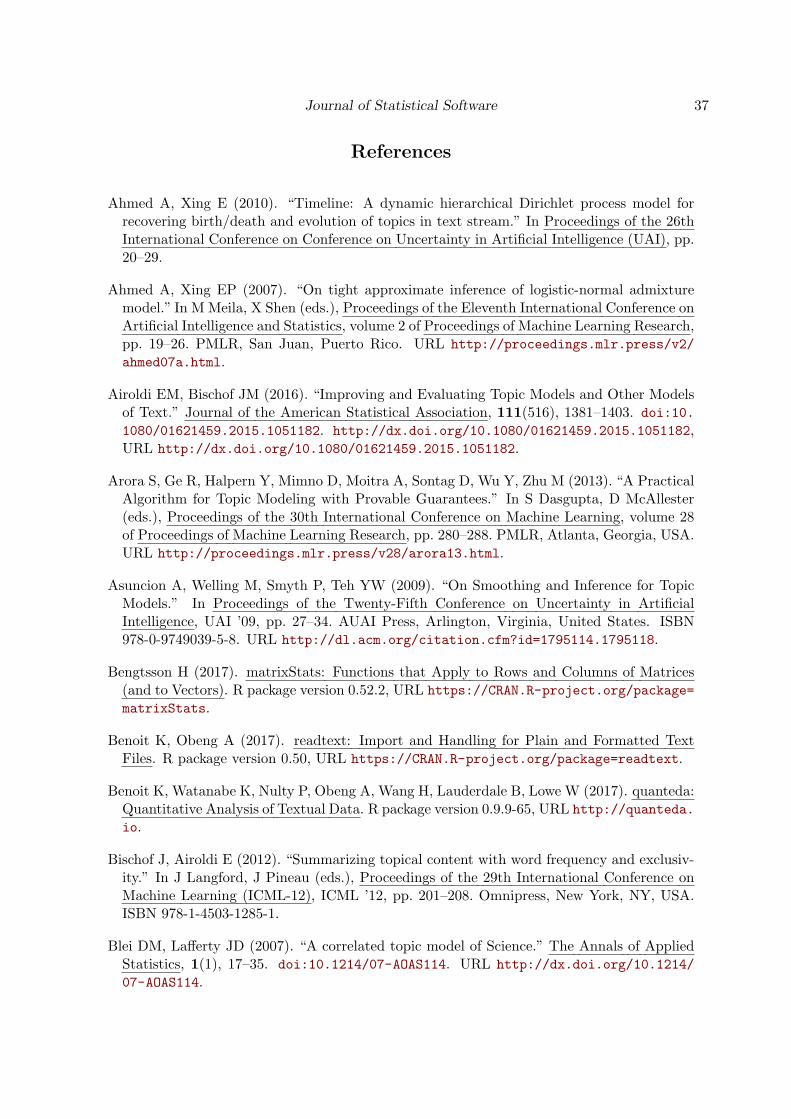
Journal of Statistical Software 37
References
Ahmed A, Xing E (2010). “Timeline: A dynamic hierarchical Dirichlet process model forrecovering birth/death and evolution of topics in text stream.” In Proceedings of the 26thInternational Conference on Conference on Uncertainty in Artificial Intelligence (UAI), pp.20–29.
Ahmed A, Xing EP (2007). “On tight approximate inference of logistic-normal admixturemodel.” In M Meila, X Shen (eds.), Proceedings of the Eleventh International Conference onArtificial Intelligence and Statistics, volume 2 of Proceedings of Machine Learning Research,pp. 19–26. PMLR, San Juan, Puerto Rico. URL http://proceedings.mlr.press/v2/
ahmed07a.html.
Airoldi EM, Bischof JM (2016). “Improving and Evaluating Topic Models and Other Modelsof Text.” Journal of the American Statistical Association, 111(516), 1381–1403. doi:10.
1080/01621459.2015.1051182. http://dx.doi.org/10.1080/01621459.2015.1051182,URL http://dx.doi.org/10.1080/01621459.2015.1051182.
Arora S, Ge R, Halpern Y, Mimno D, Moitra A, Sontag D, Wu Y, Zhu M (2013). “A PracticalAlgorithm for Topic Modeling with Provable Guarantees.” In S Dasgupta, D McAllester(eds.), Proceedings of the 30th International Conference on Machine Learning, volume 28of Proceedings of Machine Learning Research, pp. 280–288. PMLR, Atlanta, Georgia, USA.URL http://proceedings.mlr.press/v28/arora13.html.
Asuncion A, Welling M, Smyth P, Teh YW (2009). “On Smoothing and Inference for TopicModels.” In Proceedings of the Twenty-Fifth Conference on Uncertainty in ArtificialIntelligence, UAI ’09, pp. 27–34. AUAI Press, Arlington, Virginia, United States. ISBN978-0-9749039-5-8. URL http://dl.acm.org/citation.cfm?id=1795114.1795118.
Bengtsson H (2017). matrixStats: Functions that Apply to Rows and Columns of Matrices(and to Vectors). R package version 0.52.2, URL https://CRAN.R-project.org/package=
matrixStats.
Benoit K, Obeng A (2017). readtext: Import and Handling for Plain and Formatted TextFiles. R package version 0.50, URL https://CRAN.R-project.org/package=readtext.
Benoit K, Watanabe K, Nulty P, Obeng A, Wang H, Lauderdale B, Lowe W (2017). quanteda:Quantitative Analysis of Textual Data. R package version 0.9.9-65, URL http://quanteda.
io.
Bischof J, Airoldi E (2012). “Summarizing topical content with word frequency and exclusiv-ity.” In J Langford, J Pineau (eds.), Proceedings of the 29th International Conference onMachine Learning (ICML-12), ICML ’12, pp. 201–208. Omnipress, New York, NY, USA.ISBN 978-1-4503-1285-1.
Blei DM, Lafferty JD (2007). “A correlated topic model of Science.” The Annals of AppliedStatistics, 1(1), 17–35. doi:10.1214/07-AOAS114. URL http://dx.doi.org/10.1214/
07-AOAS114.

38 Structural Topic Models
Blei DM, Ng A, Jordan M (2003). “Latent Dirichlet Allocation.” Journal of Machine LearningResearch, 3, 993–1022.
Bouchet-Valat M (2014). SnowballC: Snowball Stemmers Based on the C Libstemmer UTF-8Library. R package version 0.5.1, URL http://CRAN.R-project.org/package=SnowballC.
Chang J (2015). lda: Collapsed Gibbs Sampling Methods for Topic Models. R package version1.4.2, URL https://CRAN.R-project.org/package=lda.
Csardi G, Nepusz T (2006). “The igraph Software Package for Complex Network Research.”InterJournal, Complex Systems, 1695(5), 1–9.
Dowle M, Srinivasan A (2017). data.table: Extension of ‘data.frame‘. R package version1.10.4, URL https://CRAN.R-project.org/package=data.table.
Eddelbuettel D, Francois R (2011). “Rcpp: Seamless R and C++ Integration.” Journal ofStatistical Software, Articles, 40(8), 1–18. ISSN 1548-7660. doi:10.18637/jss.v040.i08.URL https://www.jstatsoft.org/v040/i08.
Eddelbuettel D, Sanderson C (2014). “RcppArmadillo: Accelerating R with High-PerformanceC++ Linear Algebra.” Computational Statistics and Data Analysis, 71, 1054–1063.
Eisenstein J, Ahmed A, Xing E (2011). “Sparse Additive Generative Models of Text.” InProceedings of the 28th International Conference on Machine Learning, pp. 1041–1048.
Eisenstein J, O’Connor B, Smith N, Xing E (2010). “A latent variable model for geographiclexical variation.” In Proceedings of the 2010 Conference on Empirical Methods in NaturalLanguage Processing, pp. 1277–1287. Association for Computational Linguistics.
Eisenstein J, Xing E (2010). The CMU 2008 Political Blog Corpus. Carnegie Mellon Univer-sity.
Feinerer I, Hornik K, Meyer D (2008). “Text Mining Infrastructure in R.” Journal of StatisticalSoftware, Articles, 25(5), 1–54. ISSN 1548-7660. doi:10.18637/jss.v025.i05. URLhttps://www.jstatsoft.org/v025/i05.
Fellows I (2014). wordcloud: Word Clouds. R package version 2.5, URL http://CRAN.
R-project.org/package=wordcloud.
Foulds J, Kumar S, Getoor L (2015). “Latent topic networks: A versatile probabilistic pro-gramming framework for topic models.” In International Conference on Machine Learning,pp. 777–786.
Friedman J, Hastie T, Tibshirani R (2010). “Regularization Paths for Generalized LinearModels via Coordinate Descent.” Journal of Statistical Software, Articles, 33(1), 1–22. ISSN1548-7660. doi:10.18637/jss.v033.i01. URL https://www.jstatsoft.org/v033/i01.
Gerrish S, Blei D (2012). “How They Vote: Issue-Adjusted Models of Legislative Behavior.”In Advances in Neural Information Processing Systems 25, pp. 2762–2770.
Grimmer J (2010). “A Bayesian hierarchical topic model for political texts: Measuring ex-pressed agendas in Senate press releases.” Political Analysis, 18(1), 1–35.

Journal of Statistical Software 39
Grimmer J, Stewart BM (2013). “Text as Data: The Promise and Pitfalls of AutomaticContent Analysis Methods for Political Texts.” Political Analysis, 21(3), 267–297.
Grun B, Hornik K (2011). “topicmodels: An R Package for Fitting Topic Models.” Journalof Statistical Software, Articles, 40(13), 1–30. ISSN 1548-7660. doi:10.18637/jss.v040.i13. URL https://www.jstatsoft.org/v040/i13.
Habel K, Grasman R, Stahel A, Stahel A, Sterratt DC (2015). geometry: Mesh Generationand Surface Tesselation. R package version 0.3-6, URL http://CRAN.R-project.org/
package=geometry.
Hausser J, Strimmer K (2009). “Entropy inference and the James-Stein estimator, withapplication to nonlinear gene association networks.” Journal of Machine Learning Research,10(Jul), 1469–1484.
Hoffman MD, Blei DM, Wang C, Paisley JW (2013). “Stochastic variational inference.”Journal of Machine Learning Research, 14(1), 1303–1347.
Hornik K (2005). “A CLUE for CLUster Ensembles.” Journal of Statistical Software,Articles, 14(12), 1–25. ISSN 1548-7660. doi:10.18637/jss.v014.i12. URL https:
//www.jstatsoft.org/v014/i12.
Hornik K, Meyer D, Buchta C (2016). slam: Sparse Lightweight Arrays and Matrices. Rpackage version 0.1-40, URL https://CRAN.R-project.org/package=slam.
Hughes MC, Sudderth E (2013). “Memoized Online Variational Inference for Dirich-let Process Mixture Models.” In CJC Burges, L Bottou, M Welling, Z Ghahra-mani, KQ Weinberger (eds.), Advances in Neural Information Processing Systems26, pp. 1133–1141. Curran Associates, Inc. URL http://papers.nips.cc/paper/
4969-memoized-online-variational-inference-for-dirichlet-process-mixture-models.
pdf.
Khan ME, Bouchard G (2009). “Variational EM Algorithms for Correlated Topic Models.”Technical report, University of British Columbia.
Krijthe JH (2015). Rtsne: T-Distributed Stochastic Neighbor Embedding using Barnes-HutImplementation. R package version 0.13, URL https://github.com/jkrijthe/Rtsne.
Lee M, Mimno D (2014). “Low-dimensional Embeddings for Interpretable Anchor-basedTopic Inference.” In Proceedings of the 2014 Conference on Empirical Methods in NaturalLanguage Processing (EMNLP), pp. 1319–1328. Association for Computational Linguistics,Doha, Qatar. URL http://www.aclweb.org/anthology/D14-1138.
Lucas C, Nielsen R, Roberts M, Stewart B, Storer A, Tingley D (2015). “Computer AssistedText Analysis for Comparative Politics.” Political Analysis, 23(2), 254–277.
Milner HV, Tingley DH (2015). Sailing the Water’s Edge: Domestic Politics and AmericanForeign Policy. Princeton University Press.
Mimno D, McCallum A (2008). “Topic models conditioned on arbitrary features withDirichlet-multinomial regression.” In Proceedings of the Twenty-Fourth Conference AnnualConference on Uncertainty in Artificial Intelligence (UAI-08), pp. 411–418. AUAI Press.
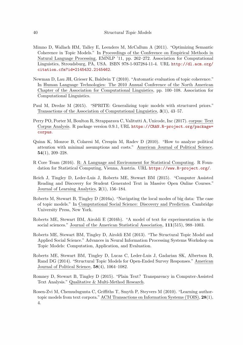
40 Structural Topic Models
Mimno D, Wallach HM, Talley E, Leenders M, McCallum A (2011). “Optimizing SemanticCoherence in Topic Models.” In Proceedings of the Conference on Empirical Methods inNatural Language Processing, EMNLP ’11, pp. 262–272. Association for ComputationalLinguistics, Stroudsburg, PA, USA. ISBN 978-1-937284-11-4. URL http://dl.acm.org/
citation.cfm?id=2145432.2145462.
Newman D, Lau JH, Grieser K, Baldwin T (2010). “Automatic evaluation of topic coherence.”In Human Language Technologies: The 2010 Annual Conference of the North AmericanChapter of the Association for Computational Linguistics, pp. 100–108. Association forComputational Linguistics.
Paul M, Dredze M (2015). “SPRITE: Generalizing topic models with structured priors.”Transactions of the Association of Computational Linguistics, 3(1), 43–57.
Perry PO, Porter M, Boulton R, Strapparava C, Valitutti A, Unicode, Inc (2017). corpus: TextCorpus Analysis. R package version 0.9.1, URL https://CRAN.R-project.org/package=
corpus.
Quinn K, Monroe B, Colaresi M, Crespin M, Radev D (2010). “How to analyze politicalattention with minimal assumptions and costs.” American Journal of Political Science,54(1), 209–228.
R Core Team (2016). R: A Language and Environment for Statistical Computing. R Foun-dation for Statistical Computing, Vienna, Austria. URL https://www.R-project.org/.
Reich J, Tingley D, Leder-Luis J, Roberts ME, Stewart BM (2015). “Computer AssistedReading and Discovery for Student Generated Text in Massive Open Online Courses.”Journal of Learning Analytics, 2(1), 156–184.
Roberts M, Stewart B, Tingley D (2016a). “Navigating the local modes of big data: The caseof topic models.” In Computational Social Science: Discovery and Prediction. CambridgeUniversity Press, New York.
Roberts ME, Stewart BM, Airoldi E (2016b). “A model of text for experimentation in thesocial sciences.” Journal of the American Statistical Association, 111(515), 988–1003.
Roberts ME, Stewart BM, Tingley D, Airoldi EM (2013). “The Structural Topic Model andApplied Social Science.” Advances in Neural Information Processing Systems Workshop onTopic Models: Computation, Application, and Evaluation.
Roberts ME, Stewart BM, Tingley D, Lucas C, Leder-Luis J, Gadarian SK, Albertson B,Rand DG (2014). “Structural Topic Models for Open-Ended Survey Responses.” AmericanJournal of Political Science, 58(4), 1064–1082.
Romney D, Stewart B, Tingley D (2015). “Plain Text? Transparency in Computer-AssistedText Analysis.” Qualitative & Multi-Method Research.
Rosen-Zvi M, Chemudugunta C, Griffiths T, Smyth P, Steyvers M (2010). “Learning author-topic models from text corpora.”ACM Transactions on Information Systems (TOIS), 28(1),4.

Journal of Statistical Software 41
Sievert C, Shirley K (2015). LDAvis: Interactive Visualization of Topic Models. R packageversion 0.3.2, URL https://CRAN.R-project.org/package=LDAvis.
Socher R, Gershman S, Perotte A, Sederberg P, Blei D, Norman K (2009). “A bayesiananalysis of dynamics in free recall.” Advances in neural information processing systems,22, 1714–1722.
Taddy M (2013). “Multinomial Inverse Regression for Text Analysis.” Journal of the AmericanStatistical Association, 108(503), 755–770.
Taddy M (2015). “Distributed multinomial regression.” Ann. Appl. Stat., 9(3), 1394–1414.doi:10.1214/15-AOAS831. URL http://dx.doi.org/10.1214/15-AOAS831.
Taddy MA (2012). “On Estimation and Selection for Topic Models.” In Proceedings of the15th International Conference on Artificial Intelligence and Statistics.
Van Der Maaten L (2014). “Accelerating t-sne using Tree-based Algorithms.” The Journal ofMachine Learning Research, 15(1), 3221–3245.
Wallach HM, Murray I, Salakhutdinov R, Mimno D (2009). “Evaluation Methods for TopicModels.” In Proceedings of the 26th Annual International Conference on Machine Learning,pp. 1105–1112. ACM.
Wand M (2015). KernSmooth: Functions for Kernel Smoothing Supporting Wand andJones (1995). R package version 2.23-15, URL http://CRAN.R-project.org/package=
KernSmooth.
Wang C, Blei DM (2013). “Variational Inference in Nonconjugate Models.” The Journal ofMachine Learning Research, 14(1), 1005–1031.
Wickham H (2017). stringr: Simple, Consistent Wrappers for Common String Operations.R package version 1.2.0, URL http://CRAN.R-project.org/package=stringr.
Zhao T, Liu H, Roeder K, Lafferty J, Wasserman L (2012). “The Huge Package forHigh-dimensional Undirected Graph Estimation in R.” The Journal of Machine LearningResearch, 13(1), 1059–1062.

42 Structural Topic Models
Affiliation:
Margaret E. RobertsDepartment of Political ScienceUniversity of California, San DiegoSocial Sciences Building 3019500 Gillman Drive, 0521, La Jolla, CA, 92093-0521E-mail: [email protected]: http://www.margaretroberts.net
Brandon M. StewartDepartment of SociologyPrinceton University149 Wallace Hall, Princeton, NJ 08544E-mail: [email protected]: brandonstewart.org
Dustin TingleyDepartment of GovernmentHarvard University1737 Cambridge St, Cambridge, MA, USAE-mail: [email protected]: http://scholar.harvard.edu/dtingley
Journal of Statistical Software http://www.jstatsoft.org/
published by the Foundation for Open Access Statistics http://www.foastat.org/
MMMMMM YYYY, Volume VV, Issue II Submitted: yyyy-mm-dddoi:10.18637/jss.v000.i00 Accepted: yyyy-mm-dd