Journal of Petroleum Science and Engineering 107 (2013) 1–11

Contents lists available at SciVerse ScienceDirect

Journal of Petroleum Science and Engineering

0920-41http://d

n CorrCenter oBeijingfax: +86

E-mpwinter(P. Fakc

journal homepage: www.elsevier.com/locate/petrol

A novel fully-coupled flow and geomechanics model in enhancedgeothermal reservoirs

Litang Hu a,b,n, Philip H. Winterfeld b, Perapon Fakcharoenphol b, Yu-Shu Wub

a College of Water Sciences, Engineering Research Center of Groundwater Pollution Control and Remediation of Ministry of Education,Beijing Normal University, Beijing 100875, PR Chinab Petroleum Engineering Department, Colorado School of Mines, Golden, CO 80401, USA

a r t i c l e i n f o

Article history:Received 5 June 2012Accepted 26 April 2013Available online 7 May 2013

Keywords:stress-sensitive formationthermo-elasticityenhanced geothermal systems (EGS)geothermal reservoir simulationcoupled thermalhydrologicmechanical (THM) model

05/$ - see front matter & 2013 Elsevier B.V. Ax.doi.org/10.1016/j.petrol.2013.04.005

esponding author at: College of Water Scif Groundwater Pollution Control and RemediaNormal University, Beijing 100875, PR Ch10 5880 2739.ail addresses: litanghu@bnu.edu.cn (L. Hu),f@mines.edu (P.H. Winterfeld), pfakchar@mymharoenphol), ywu@mines.edu (Y.-S. Wu).

a b s t r a c t

The geomechanical behavior of porous media has become increasingly important in stress-sensitivereservoirs. This paper presents a novel fully-coupled fluid flow-geomechanical model (TOUGH2-EGS).The fluid flow portion of our model is based on the general-purpose numerical simulator TOUGH2-EOS3.The geomechanical portion is developed from linear elastic theory for a thermo-poro-elastic systemusing the Navier equation. Fluid flow and geomechanics are fully coupled, and the integral finite-difference method is used to solve the flow and stress equations. In addition, porosity and permeabilitydepend on effective stress and correlations describing that dependence are incorporated into thesimulator. TOUGH2-EGS is verified against analytical solutions for temperature-induced deformation andpressure-induced flow and deformation. Finally the model is applied to analyze pressure andtemperature changes and deformation at The Geysers geothermal field. The results demonstrate thatthe model can be used for field-scale reservoir simulation with fluid flow and geomechanical effects.

& 2013 Elsevier B.V. All rights reserved.

1. Introduction

In the past, reservoir engineers has neglected geomechanicaleffects when considering porous media fluid flow because of littlechange in rock properties or deformation in conventional reservoirs.However, geomechanical effects should not be ignored in manyinstances related to enhanced geothermal systems, such as analyzinghigh flow rate drive oil recovery, associated formation subsidence,stress sensitive fractured reservoirs, and dealing with wellbore stabi-lity, and production of heavy oil (Merle et al., 1976; Kosloff et al., 1980;Lewis and Schrefler, 1998; Settari and Walters, 2001; Samier andGennaro, 2008; Boutt et al., 2011). The coupling of geomechanics withporous media fluid and heat flow is of importance in a variety oftechnical venues. Some examples are soil shrinkage from waterevaporation and soil heaving due to water freezing; formationpermeability and porosity changes and ground surface uplift fromsubsurface CO2 sequestration in a saturated geologic formation; androck deformation associated with heavy oil recovery processes such as

ll rights reserved.

ences, Engineering Researchtion of Ministry of Education,ina. Tel.: +86 138 1116 3348;

ail.mines.edu

steam assisted gravity drainage or from cold water injection and hotwater production in geothermal fields.

Models with coupled flow and geomechanics can be classified intofour types: fully coupled, iteratively coupled, explicitly coupled, andloosely coupled (Settari and Walters, 2001; Longuemare et al., 2002;Minkoff et al., 2003; Tran et al., 2004; Samier and Gennaro, 2008). Fora fully coupled simulator, a set of equations (generally a large systemof nonlinear coupled partial differential equations) incorporating all ofthe relevant physics must be derived (Minkoff et al., 2003). Theiterative coupling method solves the pore fluid flow variables andthe geomechanical conditions independently and sequentially. Theiterative coupling between the reservoir simulator and the geomecha-nical model is then performed at the end of each timestep throughpore volume calculations (Longuemare et al., 2002). The explicitlycoupled method is a special case of the iteratively coupled method inwhich only one iteration per one time increment is performed. Inloose coupling, there are two sets of equations which are solvedindependently, but information is passed at designated time intervalsin both directions between fluid flow and geomechanics simulators(Minkoff et al., 2003). In the fully coupled method the equations offlow and geomechanics are solved simultaneously at each time step. Inthe iteratively coupled method, either the flow or mechanical problemis solved first, and then the other equation is solved iteratively usingthat intermediate solution information (GEOSIM (Settari et al., 2000),GeoSys/Rockflow (Wang and Kolditz, 2007)). In explicitly coupledmethods, only one iteration is taken between the geomechanical andfluid flow modules, for example, ROCMAS (Noorishad et al., 1984),

Nomenclature

Anm the cross area, m2

Aj the cross area of grid j, m2

Aij the cross area between grid i and j, m2

CR heat conductivity, W K−1 m−1

Cϕ Pore compressibility, Pa−1

cs Specific heat capacity of rock, J kg−1 1C−1

ct Bulk total compressibility, Pa−1

DT Thermal diffusivity, m2s−1

E Young modulus, PaF the force, PaFκ the mass or energy transport terms along the borehole

due to advective processes, W m−1

Fκnm the mass or energy transport terms along cross sectionnm due to advective processes, W m−1

Fl l-direction body force (gravity), Pa m−1

g Gravitational acceleration constant, m s−2

h the total column height, mhβ Specific enthalpy in phase β, J kg−1

k Absolute permeability, m2

kT Heat conductivity of rock Wm−1 1C−1

K Bulk modulus, Pakr β Relative permeability to phase βM Biot's modulus, PaMκ the accumulation terms of the components and

energy κ, kg m−3

Mκn the accumulation terms of the components and

energy κ of grid n, kg m−3

n Normal vector on surface element, demensionlesst Time, sT Temperature, 1C or KTref Reference temperature, 1C or Kuβ the Darcy velocity in phase β, m s−1

Uβ the internal energy of phase β per unit mass, J kg−1

Vn Volume of the nth grid cell, m3

P Pressure, PaP0 Incremental pressure due to load, PaPc Capillary pressure, PaPc0 Reference capillary pressure, PaPβ the fluid pressure in phase β, Paqκ Source/sink terms for mass or energy components,

kg m−3 s−1

qκn Source/sink terms for mass or energy components ofgrid n, kg m−3 s−1

Rκn the residual of componentκfor grid block n, kg s−1

R4n the residual of stress for grid block n, Pa m−2

S Storage coefficient, Pa−1

Sl Saturation of liquid phase, demensionlessSβ Saturation of phase β, dimensionless

Tb Constant temperature boundary, 1CTi Initial temperature, 1Cw Vertical displacement of the upper surface, mxt Primary variables at time t, pressure, temperature, air

fraction, or stressXκβ Mass fraction of component κ in fluid phase β,

dimensionlessVb Bulk volume, m3

z Distance along-column coordinate, m

Greek letters

α Biot's coefficient, dimensionlessαP Biot's coefficient, dimensionlessαT Biot's coefficient, dimensionlessβ Linear thermal expansion coefficient, 1C−1

μβ Viscosity, Pa sμf fluid viscosity, Pa sϕ Porosity, dimensionlessλ Thermal conductivity, W K−1 m−1

λs Lame's constant, Paεll Strain components, l¼x, y, z, dimensionlessεls Strain components, ls¼xy, yz, zx, dimensionlessεil Strain components, j¼x, y, z, l¼x, y, z, dimensionlessεv Volumetric strain, dimensionlessε Strain tensor, dimensionlessu Displacement vector, mul Displacement component, l¼x,y,z, mν Poisson's ratio of rock, dimensionlessνu the undrained Poisson's ratio of rock, dimensionlesss′ Effective stress, Pasex External load per area at the top column, Paρtot the density of rock, kg m−3

ρR the density of rock grain, kg m−3

ρβ the density of phase β, kg m−3

Γ the perimeter of the cross-section, mΓn Area of closed surface, m2

τkl k¼ l for shear stress; k≠l for normal stress, k¼x, y, z,l¼x, y, z, Pa

τls Stress components, ls¼xy, yz, zx, Paτm Mean total stress, Paψ i Coefficient, dimensionless

Subscripts and Superscripts

κ the index for the components, κ¼1 (water), 2 (air),and 3 (energy)

β G for gas; L for liquid

L. Hu et al. / Journal of Petroleum Science and Engineering 107 (2013) 1–112

FRACture (Kohl and Hopkirk, 1995) and FRACON (Nguyen, 1996). Theloosely coupling method is resolved only after a certain number offlow time steps, for example, TOUGH-FLAC (Rutqvist et al., 2002;Rutqvist, 2011), ATH2VIS (Longuemare et al., 2002), Integrated ParallelAccurate Reservoir Simulator (IPARS) for flow and JAS3D for mechanics(Minkoff et al., 2003). Some models include modeling of induced slip,such as the models developed by Koh et al. (2011); Ghassemi andZhou (2011); McClure and Horne (2011). Koh et al. described thecharacteristic properties of individual fracture using finite elementmodule. Ghassemi and Zhou used both finite element method andintegral equation method in their models. McClure et al. tooksequential stimulation method (similar to iteratively coupled method)in their models.

The fully coupled method is internal consistent and rigorous,because the fluid flow and geomechanical equations are solvedsimultaneously on the same discretized grid. Consequently, consider-able effort is required to develop such a simulator (Settari andWalters,2001). Typical geomechanical models assign rock displacement orvelocity as primary variables, two primary variables for 2-D andthree primary variables for 3-D. As a result, the coupling flow-geomechanical model requires intensive computation. Various cou-pling techniques have been developed to reduce such computationaltime required.

The objective of this paper is to present a new fully-coupledmultiphase, heat flow and geomechanical model, including themathematical equations and formulation. Mean total stress is the

L. Hu et al. / Journal of Petroleum Science and Engineering 107 (2013) 1–11 3

only primary variable for geomechanical model in a 3-D problem.Thus, the computational requirement is less than that of typicalgeomechanical model. We then verify the model using twoanalytical solutions, and finally apply the model to a field example.It is assumed that the reservoir rock is linear elastic and obeys thegeneralized version of Hooke's law. The novelty of our model liesin its simplified treatment of rock deformation using the relationof mean normal stress and volumetric strain. Pressure, tempera-ture, air mass fraction, and mean total stress are solved simulta-neously for each Newton iteration. The advantages of thesimplification of typical geomechanical model lies on (1) thecomputational requirement is less than that of the typical geo-mechanical model because of less primary variable and (2) thismethod is still capable of capturing geomechanical behavior ofrock as seen in the comparison between numerical and analyticalsolution as well as in Geyser case.

2. Mathematical and numerical model

2.1. Multiphase fluid and heat flow module

The basis for our simulator is the TOUGH2/EOS3 model, whichsolves the mass and energy balance equations describing fluid andheat flow in multiphase, multi-component systems. Fluid flow isgoverned by a multiphase extension of Darcy's law and there isdiffusive mass transport in all phases. Heat flow occurs by conductionand convection, with sensible as well as latent heat effects included.The TOUGH2/EOS3 mass and energy equations for two-phase flow oftwo components (water, air) are summarized in Table 1 (see Nomen-clature for definitions of all symbols used).

2.2. Geomechanical module

This fully coupling assumes that boundaries of each element canmove as an elastic material and obey the generalized version ofHooke's law (Winterfeld and Wu, 2011). The mean total stress is anadditional primary variable. Under the assumption of linear elasticitywith small strains for a thermoporoelastic system, the equilibriumequation can be expressed as follows: (Jaeger et al., 2007)

τll−ðαP þ 3βKðT−Tref ÞÞ ¼ 2Gεll þ λsðεxx þ εyy þ εzzÞ; l¼ x; y; z ð1Þ

and the shear stresses are

τls ¼ 2Gεls; ls¼ xy; yz; zx ð2Þ

The trace of Hooke's law for a thermoporoelastic medium is

Kεv ¼ τm−αP−3βKðT−Tref Þ ð3Þ

These stress and strains are symmetric tensors. The equations of stressequilibrium are derived from a force balance on a differential volume

Table 1Equations of fluid and heat flow solved in TOUGH2-EGS.

Description Equation

Conservation of mass andenergy

ddt

RVnMκdVn ¼

RΓnFκ�ndΓn þ

RVnqκdVn κ¼1, 2,

3Mass accumulation Mκ ¼ ϕ∑

βSβρβX

κβ , κ¼1, 2

Mass flux Fκ ¼∑βXκβρβuβ , κ¼1, 2

Energy flux F3 ¼ −λ∇T þ ∑βhβρβuβ

Energy accumulation M3 ¼ ð1−ϕÞρRCRT þ ϕ∑βρβSβUβ

Phase velocity uβ ¼ −k krβρβμβ

ð∇Pβ−ρβgÞ

element. They are, when neglecting acceleration

∂τxl∂x

þ ∂τyl∂y

þ ∂τzl∂z

þ Fl ¼ 0; l¼ x; y; z ð4Þ

Strain can be expressed in terms of a displacement vector, u. Thedisplacement vector points from the new position of a volumeelement to its previous one. The strain tensor is related to thedisplacement vector by

ε ¼ 12 ∇uþ ð∇uÞTh i

ð5Þ

Each element of Eq. (5) has the form

εjl ¼12

∂ul

∂xjþ ∂uj

∂xl

� �; ðl; jÞ ¼ x; y; z; xl ¼ x; y; z ð6Þ

We then derive (see Appendix A)

3ð1−νÞð1þ νÞ∇

2τm þ ∇⋅F−2ð1−2νÞð1þ νÞ ðα∇2P þ 3βK∇2TÞ ¼ 0 ð7Þ

The boundary type of stress includes specified stress boundaryonly. Specified stress boundary remains fixed at all time steps andthe mean total stress at other places will be subjected to thepressure, temperature and body force. For 1D, 2D and 3D cases, themodel should include at least 1, 2 and 3 specified stress boundariesrespectively. For an example of 1D case, the model is discretizedinto N gridblocks, and the number of connections should be N−1.From Eq. (7), there are N−1 equations, and the number ofboundary condition should be at least 1, and so we get N equationsand N unknown mean total stress. So we can obtain mean normalstress field after solving the linear equations.

2.3. Space and times discretization

The integral finite-difference method (Pruess et al., 1999) isused to discretize the continuous space variables for numericalsimulation. Time discretization is carried out using a backward,first-order, and fully implicit finite-difference scheme. Time andspace discretization of the governing mass and energy balanceequations results in a set of coupled non-linear equations, whichcan be written in residual form as follows:

Rκnðxtþ1Þ ¼Mκ

nðxtþ1Þ−MκnðxtÞ−

ΔtVn

∑mAnmF

κnmðxtþ1Þ þ Vnqκ;tþ1

n g ¼ 0; κ¼ 1;2;3�

ð8ÞThe stress equation, Eq. (7), relates mean total stress to porepressure, temperature, and body forces. It is also discretized usingthe integral finite difference method over a volume element withan outer surface. After applying the divergence theorem to theintegral finite difference volume integral the following is obtained:Z

3ð1−νÞð1þ νÞ∇τm þ F−

2ð1−2νÞð1þ νÞ ðα∇P þ 3βK∇TÞ

� �⋅_ndΓ ¼ 0 ð9Þ

The surface integral is expressed as a discrete sum of averages oversurface segments

∑j

3ð1−νÞð1þ νÞ∇τm þ F−

2ð1−2νÞð1þ νÞ ðα∇P þ 3βK∇TÞ

� �jAj ¼ 0 ð10Þ

The boundary conditions for Eq. (10) are a reference temperature,pressure, and stress at some distance from a given grid block. Forexample, surface pressure, stress (both atmospheric) and tem-perature can be used as boundary conditions.

The finite difference approximation for Eq. (10) in residual form is

R4nðxtþ1Þ ¼∑

j

3ð1−νÞð1þ νÞ

τj−τisij

−2ð1−2νÞð1þ νÞ α

Pj−Pi

sij−

2Eð1þ νÞ β

Tj−Ti

sijþ ρtotgk̂⋅n̂

� �ij

Aij ¼ 0

ð11ÞThe model solves for four primary variables (pressure, air massfraction/gas saturation, temperature, and mean total stress) for each

Fig. 1. Model architecture of TOUGH2-EGS.

L. Hu et al. / Journal of Petroleum Science and Engineering 107 (2013) 1–114

grid block. A uniform residual form for four primary variables isshown in Eq. (12). For variables of pressure, air mass fraction/gassaturation and temperature, the residuals are formed from Eq. (8).For mean total stress, the residuals is assembled from Eq. (11).Eq. (12) are solved by the Newton/Raphson method that iteratesuntil the residuals are reduced below preset convergence criteria.

−∑i

∂Rκ;tþ1n

∂xi

���pðxi;pþ1−xi;pÞ ¼ Rκ;tþ1

n ðxi;pÞ; κ¼ 1;2;3;4 ð12Þ

2.4. Stress-dependent parameters modification

Permeability and porosity are both dependent on effectivestress according to the following relations:

s′¼ τm−αP ð13Þ

k¼ kðs′; pÞ ð14Þ

ϕ¼ ϕðs′; pÞ ð15ÞSince bulk volume is related to porosity, bulk volume depends oneffective stress and pore pressure

Vb ¼ Vbðs′; PÞ ð16ÞIn addition, permeability and porosity are used to scale capillarypressure according to the relation by Leverett (1941)

Pc ¼ Pc0

ffiffiffiffiffiffiffiffiffiffiffiffiffiffiðk=ϕÞ0

pffiffiffiffiffiffiffiffiffiffiffiffiðk=ϕÞ

p ð17Þ

where subscript 0 refers to reference conditions.The coupled multiphase flow and geomechanical model, called

TOUGH2-EGS, implements four empirical correlations for porosityas a function of effective stress (Appendix B): Zimmerman et al.(1986) for sedimentary rock, Rutqvist et al. (2002) for sedimentaryrock and fractures, and McKee et al. (1988); and five empiricalcorrelations for permeability a function of effective stress(Appendix C): Rutqvist et al. (2002) for sedimentary rock andfractures, the Carman–Kozeny equation, Ostensen (1986), andVerma and Pruess (1988).

2.5. Model architecture of TOUGH2-EGS

The model architecture is summarized in Fig. 1. There are fourprimary variables, pressure, temperature, air mass fraction, andmean total stress. Secondary variables such as liquid saturationand volumetric strain are derived from the primary variables. First,the grid systems, boundary conditions, sources and sink terms,initialization parameters of pressure, temperature, and mean totalstress are inputted to the model. The initial stress field is thencalculated based on Eq. (10) with initial pressure field, initialtemperature field and stress boundary conditions. Then, the timeiteration is carried out. During time iteration, the coefficientmatrixes for four primary variables (κ¼1, 2, 3, 4) in Eq. (12) areassembled, and then pressure, temperature, air mass fraction, andmean total stress are solved iteratively for each Newton iteration.Also, permeability and porosity correction will be carried out ineach time iteration is the module of equation of state. Thecalculation of fluid and geomechanical variables is fully implicitand fully coupled.

3. Verification of TOUGH2-EGS

Consolidation problems subjected to stress and temperaturechange will be verified. Here, three cases, 1-D consolidation, 1-Dheat conduction and 2-D consolidation (Mandel's problem), isselected for testing the applicability of our model when comparing

the simulated results with analytical solutions. The poroelastic wasverified by comparing the numerical result against the analyticalsolution of 1-D consolidation problem and the thermoelastic wasverified against the analytical solution of 1-D heat conduction.

3.1. 1-D consolidation in a porous permeable column

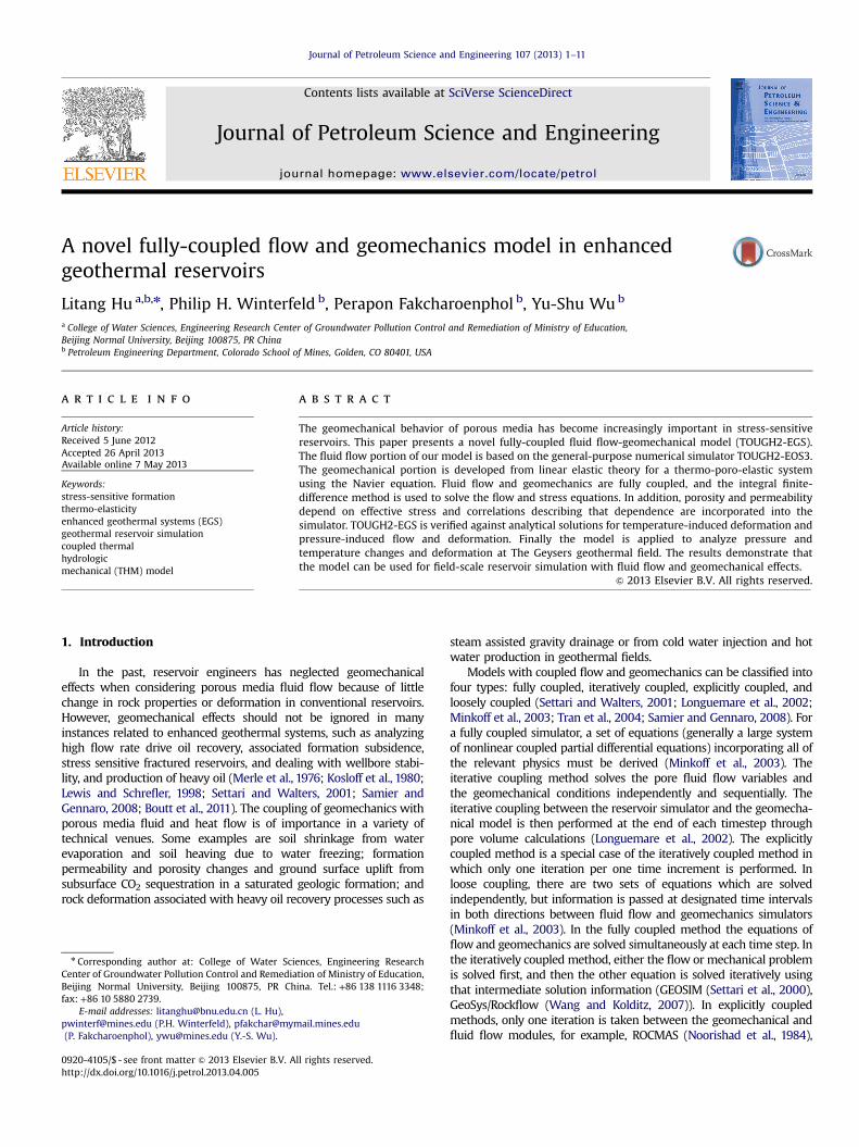
A 1-D consolidation problem is simulated numerically andcompared with Jaeger's analytical solution (Jaeger et al., 2007,listed in Appendix D) to verify the validity of the simulator code.The 1-D problem is a porous permeable column that undergoesuniaxial strain in the vertical direction only. The column issubjected to a constant load on the top (Fig. 2), the fluid boundarypressure is set to zero gauge right after the load is imposed, andonly vertical displacement takes place. Basic parameters for rockproperties, fluid properties, initial and boundary conditions can beseen in Fig. 2 and are listed in Table 2.

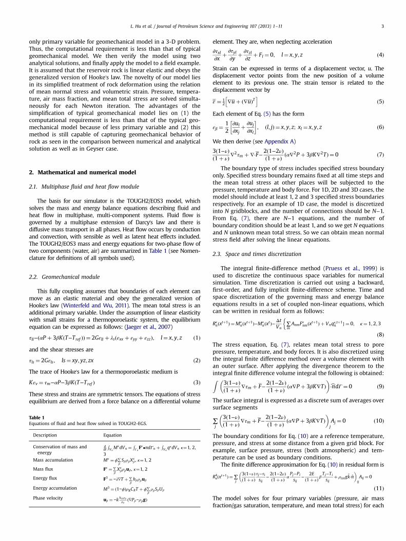
The comparison of normalized excess pressure (defined as theratio of pressure change to the maximum pressure) and verticaldisplacement between the analytical and numerical solutions inFig. 3 indicates that our numerical results produce essentially thesame answers as analytical models, which lend creditability to ourcomputational approach.

3.2. 1-D heat conduction in a deformable rock column

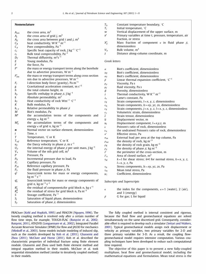
1-D heat conduction in a deformable medium is simulatednumerically and compared with Jaeger's analytical solution (Jaegeret al., 2007, listed in Appendix E) to verify the validity of thesimulator code. The 1-D problem is a non-permeable column thatundergoes uniaxial strain in the vertical direction only. Thecolumn is subjected to a constant temperature on the top(Fig. 4) and only heat conduction takes place. Input parameters

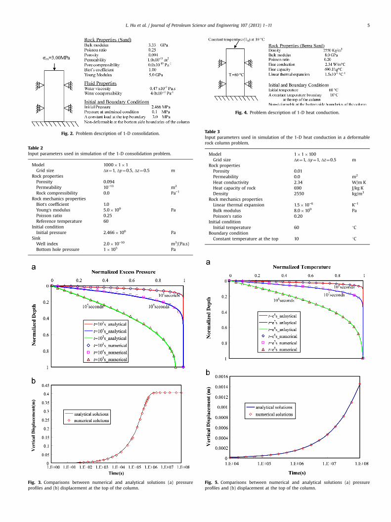
Fig. 2. Problem description of 1-D consolidation.

Table 2Input parameters used in simulation of the 1-D consolidation problem.

Model 1000�1�1Grid size Δx¼1, Δy¼0.5, Δz¼0.5 m

Rock propertiesPorosity 0.094Permeability 10−13 m2

Rock compressibility 0.0 Pa−1

Rock mechanics propertiesBiot's coefficient 1.0Young's modulus 5.0�109 PaPoisson ratio 0.25Reference temperature 60

Initial conditionInitial pressure 2.466�106 Pa

SinkWell index 2.0�10−10 m3/(Pa.s)Bottom hole pressure 1�105 Pa

Fig. 3. Comparisons between numerical and analytical solutions (a) pressureprofiles and (b) displacement at the top of the column.

Fig. 4. Problem description of 1-D heat conduction.

Table 3Input parameters used in simulation of the 1-D heat conduction in a deformablerock column problem.

Model 1�1�100Grid size Δx¼1, Δy¼1, Δz¼0.5 m

Rock propertiesPorosity 0.01Permeability 0.0 m2

Heat conductivity 2.34 W/m KHeat capacity of rock 690 J/kg KDensity 2550 kg/m3

Rock mechanics propertiesLinear thermal expansion 1.5�10−6 K−1

Bulk modulus 8.0�109 PaPoisson’s ratio 0.20

Initial conditionInitial temperature 60 1C

Boundary conditionConstant temperature at the top 10 1C

Fig. 5. Comparisons between numerical and analytical solutions (a) pressureprofiles and (b) displacement at the top of the column.

L. Hu et al. / Journal of Petroleum Science and Engineering 107 (2013) 1–11 5

L. Hu et al. / Journal of Petroleum Science and Engineering 107 (2013) 1–116

in the model are listed in Table 3. Fig. 5a and b shows the matchbetween analytical and numerical solutions are excellent.

Fig. 7. Comparison of pressure, volumetric strain between numerical and analyticalsolutions, (a) pressure, (b)volumetric strain.

3.3. Mandel's problem

The geometry of Mandel's problem is depicted in Fig. 6. Aninfinitely long specimen with a rectangular cross-section is sand-wiched between two rigid, frictionless and impermeable plates.The specimen consists of incompressible solid constituents, and itis saturated with a single-phase incompressible fluid. At initialtime, a force of 2F per unit thickness of the specimen is applied atthe top and bottom. The lateral boundary surfaces perpendicularto the x direction are traction free and exposed to the ambientpressure. As predicted by the Skempton effect, a uniform pressurerise will be observed inside the specimen upon the exertionof a force 2F on the rigid plates. As time passes on, pore pressurenear these boundaries must dissipate due to drainage access.Abousleiman et al. (1996) extend the classical problem to accountfor transversely isotropic material (the analytical solution is shownin Appendix F). Table 4 gives the dimensions of the specimen andits material properties used in this simulation (Fakcharoenpholet al., 2012). Fig. 7a and b shows the comparison of pressure at thecenter of the specimen, volumetric strain at the right and top edgeof the specimen between numerical and analytical solutions. Thepressure curve at the center has a peak and shows a goodagreement with analytical solutions.

Fig. 6. Mandel's problem description.

Table 4Input parameters for Mandel's problem.

Model 1000�1000�100Grid size Δx¼10, Δy ¼10, Δz¼100 mSize 1000�1000 m2

Applied stress 1470 MPaRock and fluid properties

Porosity 0.094Permeability 1.0e−13 m2

Pore compressibility 0.0Rock mechanics properties

Young’s modulus 5.0�109 Pa.sBiot's coefficient 1.0Poisson's ratio 0.25

Initial conditionInitial pressure 3.0�106 Pa

4. Model application

The Geysers is the site of the largest geothermal electricitygene`rating operation in the world and has been in commercialproduction since 1960 (Mossop and Segall, 1997, 1999; Rutqvist andTsang, 2002; Rutqvist et al., 2006a, 2006b; Rutqvist and Oldenburg,2008; Khan and Truschel, 2010; Rutqvist, 2011). It is a vapor-dominated geothermal reservoir system that is hydraulically con-fined by low permeability rock. As a result of high steam withdrawalrates, the reservoir pressure declined until the mid 1990s, whenincreasing water injection rates resulted in a stabilization of thesteam reservoir pressure. Archival INSAR images were acquired fromapproximately monthly satellite passes over the region for a seven-year period, seven-year period, from 1992 to 1999, and the data iscompared with displacement calculated from our model.

The combined effects of steam production and water injection in44 years and their influences on the ground deformation will beanalyzed. Based on the work by Rutqvist et al. (2008) and Rutqvistet al. (2010), a cross-axis (NE-SW) two-dimensional model grid of theGeysers Geothermal Field was established. Permeability, tempera-ture, and boundary conditions are shown in Fig. 8. The initial thermaland hydrological conditions (vertical distributions of temperature,pressure and liquid saturation) are typically established throughsteady-state multi-phase flow simulations. According to previousstudies, the adopted rock-mass bulk modulus is 3 GPa and the linearthermal expansion coefficient is 3�10−5 1C−1. Pore compressibilityand the reservoir Poisson's ratio of the reservoir is 1.0�10−10 Pa−1

and 0.25, respectively. The injection well is about 217.5 m away fromthe production well. The steam-production and water-injection rateused in the model is estimated from the field-wide production andinjection data (Mossop and Segall, 1997; Majer and Peterson, 2007;Khan and Truschel, 2010; Sanyal and Enedy, 2011).

4.1. Change of pressure and temperature after 44 years

Fig. 9 shows calculated liquid saturation and changes in fluidpressure and temperature after 44 years of production andinjection. Fig. 9a shows the injection caused formation of a wetzone that extends towards 1000 m. Fig. 9b demonstrates pressuredecrement is about 2�106 Pa after steam production and waterinjection. Fig. 9c indicates a local cooling effect and the maximum

L. Hu et al. / Journal of Petroleum Science and Engineering 107 (2013) 1–11 7

temperature decrement is about 50 1C. All the results are almostthe same as the results from Rutqvist et al. (2008).

4.2. Changes in stress and volumetric strain

Fig. 10a and b displays changes in mean total stress andvolumetric strain, respectively. The mean total stress change in

Fig. 8. Half-symmetric model domain with hydraulic prop

Fig. 9. Simulated profile of liquid saturation (a), changes in fluid pressure (b), c

Fig. 10. Simulated changes in mean total stress (a) and volum

the rock mass depends on the production-induced depletion andinjection-induced cooling. The change in mean total stress is about0.5–1.5 MPa and the volumetric strain is about 0.0001–0.0004. It isassumed that the length in x, y, and z directions will be changeduniformly and the ground displacement can be obtained from thevolumetric strain and volume. Fig. 11 shows the change ofsimulated ground displacement with time and the comparison

erties and boundary conditions (Rutqvist et al., 2008).

hanges in temperature and (c) after 44 years of production and injection.

etric strain (2) after 44 years of production and injection.

Fig. 11. Comparison of calculated and INSAR evaluated vertical displacements andsimulated results from TOUGH2-FLAC from year 1992 to 1999 since start of steamproduction.

Fig. 12. Comparison of calculated and INSAR evaluated total subsidence andsimulated results from TOUGH2-FLAC from 1992 to 1999 along the cross sectionof model.

L. Hu et al. / Journal of Petroleum Science and Engineering 107 (2013) 1–118

with INSAR data and results from TOUGH2-FLAC (Rutqvist, 2011).Fig. 12 shows the change of displacement along the cross-sectionof the model and the comparison with observed and knownsimulated results. It can be seen from these two figures that thereis good agreement between simulated ground displacement andINSAR data.

5. Conclusions

We present an efficient fully-coupled fluid flow and geome-chanics simulator (TOUGH2-EGS) for simulating multiphase flow,heat transfer and rock deformation in porous media. Our numer-ical model is verified using three problems with analytical solu-tions and the results show that our numerical model can produceessentially the same results as analytical models do. The model isapplied to the analysis of deformation at the Geyser geothermalfield, California. The model shows the changes of pressure,pressure and liquid saturation after 44 years of production andinjections, and also thermo-elastic cooling shrinkage near injec-tion and production wells is the dominant cause of stress changes.The results show that TOUGH2-EGS is rigorous in handlingcoupled flow and rock deformation and is easily applied tostress-sensible reservoirs for analyzing multiphase fluid, heat flowand rock deformation.

Compared with a numerical modeling code for advancedgeotechnical analysis of soil, rock, and structural support, such asFLAC3D and ECLIPSE, our numerical model only calculates meantotal stress as opposed to the total stress tensor, and thissimplification may be a shortcoming of our model since it cannotanalyze phenomena dependent on shear stress, such as rockfailure. This method used in this paper is a simplification of typicalgeomechanical model where the advantage lies on (1) the com-putational requirement is less than that of the typical geomecha-nical model because of less primary variable and (2) this method isstill capable of capturing geomechanical behavior of rock. This

paper is mainly concerned with fluid and heat flow and geome-chanics in porous media, and geomechanics in the fracturedreservoir is not discussed here.

Acknowledgments

This work is supported by the U.S. Department of Energy underContract no. DE-EE0002762, “Development of Advanced Thermal-Hydrological-Mechanical- Chemical (THMC) Modeling Capabilitiesfor Enhanced Geothermal Systems”. This work is also supported bythe CMG Foundation and the National Nature Science Foundationof China (Grant numbers: 41072178 and 40872159). The authorswould also like to thank Dr. Jonny Rutqvist for providing data andmodeling results in the Geyser case studies.

Appendix A. Derivations of geomechanical equation

Substituting Eqs. (1) and (6) into Eq. (5) and rearranging yieldsthe following for x-component, y-component, and z-component,respectively:

α∂P∂x

þ 3βK∂T∂x

þ ðGþ λsÞ∂2ux

∂x2þ ∂2uy

∂x∂yþ ∂2uz

∂x∂z

� �

þ G∂2ux

∂x2þ ∂2ux

∂y2þ ∂2ux

∂z2

� �þ Fx ¼ 0 ðA1Þ

α∂P∂y

þ 3βK∂T∂y

þ ðGþ λsÞ∂2ux

∂x∂yþ ∂2uy

∂y2þ ∂2uz

∂y∂z

� �

þ G∂2uy

∂x2þ ∂2uy

∂y2þ ∂2uy

∂z2

� �þ Fy ¼ 0 ðA2Þ

α∂P∂z

þ 3βK∂T∂z

þ ðGþ λsÞ∂2ux

∂x∂zþ ∂2uy

∂y∂zþ ∂2uz

∂z2

� �

þ G∂2uz

∂x2þ ∂2uz

∂y2þ ∂2uz

∂z2

� �þ Fz ¼ 0 ðA3Þ

Eqs. (A1)–(A3) can be expressed in vector notation as

α∇P þ 3βKα∇T þ ðλs þ GÞ∇ð∇⋅uÞ þ G∇2uþ F ¼ 0 ðA4Þwhich is the thermoporoelastic version of the Navier equations.

Take the partial derivative with respect to x of x-componentEq. (A1), and the analogous for Eqs. (A(2) and A3), and add thethree equations to obtain

α∂2P∂x2

þ ∂2P∂y2

þ ∂2P∂z2

� �þ ∂Fx

∂xþ ∂Fy

∂yþ ∂Fz

∂zþ 3βK

∂2T∂x2

þ ∂2T∂y2

þ ∂2T∂z2

� �

þðGþ λsÞ∂2

∂x2∂ux

∂xþ ∂uy

∂yþ ∂uz

∂z

� �þ G

∂2

∂x2þ ∂2

∂y2þ ∂2

∂z2

� �∂ux

∂x

þðGþ λsÞ∂2

∂y2∂ux

∂xþ ∂uy

∂yþ ∂uz

∂z

� �þ G

∂2

∂x2þ ∂2

∂y2þ ∂2

∂z2

� �∂uy

∂y

þðGþ λsÞ ∂2

∂z2∂ux

∂xþ ∂uy

∂yþ ∂uz

∂z

� �þ G

∂2

∂x2þ ∂2

∂y2þ ∂2

∂z2

� �∂uz

∂z¼ 0

ðA5ÞEq. (A5) written in vector notation is

α∇2P þ 3βK∇2T þ ðλs þ 2GÞ∇2ð∇⋅uÞ þ ∇⋅F ¼ 0 ðA6ÞThe divergence of the displacement vector is the volumetric strain

∇⋅u¼ ∂ux

∂xþ ∂uy

∂yþ ∂uz

∂z¼ εxx þ εyy þ εzz ¼ εv ðA7Þ

Summing Eq. (1) over x, y, and z-components gives the trace ofHooke's law for a thermoporoelastic medium. This sum is an

L. Hu et al. / Journal of Petroleum Science and Engineering 107 (2013) 1–11 9

invariant for an isotropic solid, and is

λþ 23G

� �εv ¼

τxx þ τyy þ τzz3

−αP−3βKðT−Tref Þ ¼ τm−αP−3βKðT−Tref Þ

ða8ÞSubstituting Eqs. (A(7) and A8) into Eq. (A6) yields

α∇2P þ 3βK∇2T þ λþ 2Gλþ ð2=3ÞG∇2ðτm−αP−3βKðT−Tref ÞÞ þ ∇⋅F ¼ 0 ðA9Þ

The coefficient of the third term in Eq. (A9) is only a function ofPoisson's ratio ν

λþ 2Gλþ ð2=3ÞG ¼ 3ð1−νÞ

ð1þ νÞ ðA10Þ

Eq. (A9) then becomes

3ð1−νÞð1þ νÞ∇

2τm þ ∇⋅F−2ð1−2νÞð1þ νÞ ðα∇2P þ 3βK∇2TÞ ¼ 0 ðA11Þ

Appendix B. Empirical corrections for porosity

B.1. (Zimmerman, 1986) poroelasticity

A theory of hydrostatic poroelasticity (Zimmerman et al., 1986)has been proposed that accounts for the coupling of rock deforma-tion with fluid flow inside the porous rock. Porous rock has a bulkand a pore volume, and those volumes are acted on by porepressure and mean stress. The compressibilities are written interms of those quantities.

Cbc ¼−1Vb

∂Vb

∂sm

� �p

ðB1Þ

where subscript b refers to bulk volume.Relationships between these compressibilities are derived for

an idealized porous medium and from that, dependence ofporosity on effective stress

dϕ¼ −½Cbcð1−ϕÞ−CrÞds′ ðB2Þwhere Cr is rock grain compressibility, an expression for the Biot'scoefficient

α¼ 1−Cr

CbcðB3Þ

and dependence of bulk volume on pore pressure and effectivestress

dVb ¼ −VbCbcds′þ CrdP ðB4Þ

B.2. Rutqvist et al. (2002), sedimentary rock

Rutqvist et al. (2002) presented the following function forporosity, obtained from laboratory experiments on sedimentaryrock by Davies and Davies (1999)

ϕ¼ ϕr þ ðϕ0−ϕrÞe−αs′ B5

where ϕ0 is zero effective stress porosity, ϕr is high effective stressporosity, and the exponent a is a parameter.

B.3. Rutqvist et al. (2002), fractures

For fractured media, they defined an aperture width bk fordirection k as

bk ¼ b0;k þ Δbkðe−ds′−e−ds′0 Þ; k¼ x; y; z ðB6Þ

where subscript 0 refers to initial conditions, Δbk is the aperturechange, and the exponent d is a parameter. Porosity is correlated

to changes in bk as

ϕ¼ ϕ0b1 þ b2 þ b3

b1;0 þ b2;0 þ b3;0ðB7Þ

B.4. McKee (1988)

McKee et al. (1988) derived a relationship between porosityand effective stress from hydrostatic poroelasticity theory byassuming incompressible rock grains

ϕ¼ ϕ0e−cpðs′−s

′0Þ

1−ϕ0ð1−e−cpðs′−s′0ÞÞ

ðB8Þ

where Cp is average pore compressibility.

Appendix C. Permeability correlations

C.1. Rutqvist et al. (2002), sedimentary rock

An associated function for permeability in terms of porosity is

k¼ k0ecððϕ=ϕ0Þ−1Þ ðC1Þwhere k0 is zero stress permeability and the exponent c is aparameter.

C.2. Rutqvist et al. (2002), fractures

Direction k permeability is correlated to fracture aperture ofother directions l and m as

kk ¼ kk;0b3l þ b3mb3l;0 þ b3m;0

ðC2Þ

C.3. Carman–Kozeny

A relationship between permeability and effective stress wasobtained from the Carman–Kozeny equation

k∝ϕ3

ð1−ϕÞ2ðC3Þ

and the above relationship for porosity. These relationships fitlaboratory and field data for granite, sandstone, clay, and coal.

C.4. Ostensen (1986)

Ostensen (1986) studied the relationship between effectivestress and permeability for tight gas sands and approximatedpermeability as

kn ¼Dlns′;n

s′ðC4Þ

where n is 0.5, D is a parameter, and s′;nis effective stress for zeropermeability, obtained by extrapolating measured square rootpermeability versus effective stress on a semi-log plot.

C.5. Verma and Pruess (1988)

Verma and Pruess (1988) presented a power law expressionrelating permeability to porosity

k−kck0−kc

¼ ð ϕ−ϕc

ϕ0−ϕcÞn ðC5Þ

where kc and ϕc are asymptotic values of permeability andporosity, respectively, and exponent n is a parameter.

L. Hu et al. / Journal of Petroleum Science and Engineering 107 (2013) 1–1110

Appendix D. Analytical solutions for 1D consolidation problem

The anlaytical solution for the 1-D consolidation problemfollows:

Pressure during drained conditions is

Pðz; tÞ ¼ P0 ∑∞

n ¼ 1;3;::

4nπ

sinnπz2h

exp

−n2π2kt

4μSh2

!ðD1Þ

Vertical displacement of the upper surface is

wðz¼ 0; tÞ ¼ sexhðλþ 2GÞ 1−

α2PMðλþ 2Gþ α2PMÞ ∑

∞

n ¼ 1;3;::

8n2π2

exp−n2π2kt

4μSh2

!" #

ðD2Þwhere

P0 ¼αPM

ðλþ 2Gþ α2PMÞ sex ðD3Þ

M¼ 1ϕct

ðD4Þ

S¼ 1M

þ α2Pλþ 2G

ðD5Þ

Appendix E. Analytical solutions for 1D heat conductionproblem

The analytical solution for the 1-D heat conduction problemfollows:

Temperature during the cooling is:

Tðz; tÞ ¼ Tb þ ðTi−TbÞerf czffiffiffiffiffiffiffiffiffiffiffi4DTt

p !

ðE1Þ

The vertical displacement is

wðz¼ 0; tÞ ¼−βð1þ νÞðTi−TbÞ

ð1−νÞ h� erf chffiffiffiffiffiffiffiffiffiffiffi4DTt

p !

þexp −h2=ð4DTtÞ

−1ffiffiffiffiffiffiffiffiffiffiffiffiffiffiffiffiffiffiffi

π=ð4DTtÞp

24

35 ðE2Þ

Appendix F. Analytical solutions for Mandel's problem

The original Mandel's solutions (1953) provides only theanalytical form for the pore pressure. Later, Abousleiman et al.(1996) extend the solution to all field quantities for materials withtransverse isotropy, as well as compressible pore fluid and solidconstitutes. The solutions are given as the following.

Pressure solution

pðx; tÞ ¼ 2FaA1

∑∞

i ¼ 1

sinðψ iÞψ i−sinðψ iÞcosðψ iÞ

ðcosðψ ix=aÞ−cosðψ iÞÞexp −ψ2i cta2

� �� �

ðF1Þwhere a is dimension of specimen, 2F is force applied to the top ofthe specimen (Pa), ψ i is an infinite series defined by tanψ i=ψ i ¼A1=A2, x is location of interest (m), t is time (s)

A1 ¼α1

2M33−2α1α2M13 þ α32M11

α3M11−α1M13þ M11M33−M13

2

M α3M11−α1M13ð Þ ðF2Þ

A2 ¼α3M11−α1M33

M11

where αi is Biot constant of direction QUOTE and Mij is drainedelastic modulus defined as

M11 ¼M33 ¼Eð1−νÞ1−ν−2ν2

M13 ¼Eν

1−ν−2ν2

and, c1 is fluid flow and mechanical properties of the specimendefined as

c1 ¼k1MM11

μf Mu11

where k1 is permeability in the x-direction, M is the Biot modulusdefined as ϕctð Þ−1, μ is fluid viscosity, and Mu

11 is undrained elasticmodulus in the x-direction defined as Mu

11 ¼M11 þ α21MDisplacement solutions:x-direction

uxðx; tÞ ¼−Fa

M13

M11M33−M213

−Fa

α1α3M þM13

A1Mðα3M11−α1M13Þ

(

� ∑∞

i ¼ 1

sinðψ iÞcosðψ iÞψ i−sinðψ iÞcosðψ iÞ

exp −ψ2i c1ta2

� �� �)x

−2Fα1A2M11

∑∞

i ¼ 1

cosðψ iÞsinðψ ix=aÞψ i−sinðψ iÞcosðψ iÞ

exp −ψ2i c1ta2

� �� �

z-direction

uzðz; tÞ ¼Fa

M11

M11M33−M213

1þ 2A2

A1−1

� �� �

� ∑∞

i ¼ 1

sinðψ iÞcosðψ iÞψ i−sinðψ iÞcosðψ iÞ

exp −ψ2i c1ta2

� �� �z

Volumetric strain

εv ¼ 1−ð1−ux=xÞð1−uy=yÞ

References

Abousleiman, Y.A., Cheng, H.-D., Detournay, E., Cui, L., Roegiers, J.-C., 1996. Mandel'sproblem revisited. Géotechnique 46 (2), 187–195.

Boutt, D.F., Cook, B.K., Williams, J.R., 2011. A coupled fluid–solid model for problemsin geomechanics: application to sand production. Int. J. Numer. Anal. methodsGeomech. 35, 997–1018.

Fakcharoenphol, P., Hu, L.T., Wu, Y.-S., 2012. Fully-implicit flow and geomechanicsmodel: application for enhanced geothermal reservoir simulations. Proceedingsof Thirty-Seventh Workshop on Geothermal Reservoir Engineering, StandfordUniveristy, Standford, California, pp. 1–10. SGP-TR-194.

Ghassemi, A., Zhou, X., 2011. A three-dimensional thermo-poroelastic model forfracture response to injection/extraction in enhanced geothermal systems.Geothermics 40 (1), 39–49.

Jaeger, J.C., Cook, N.G.W., Zimmerman, R.W., 2007. Fundamentals of RockMechanics, 4th ed. Blackwell Publishing, Malden, MA, USA.

Khan, M.A., Truschel, J., 2010. The Geysers geothermal field, an injection successstory. GRC Transactions, 1239–1242.

Koh, J., Roshan, H., Rahman, S.S., 2011. A numerical study on the long term thermo-poroelastic effects of cold water injection into naturally fractured geothermalreservoirs. Comput. Geotechnics 38 (5), 669–682.

Kohl, T., Hopkirk, R.J., 1995. The finite element program “FRACTure” for thesimulation of hot dry rock reservoir behavior. Geothermics 24, 345–359.

Kosloff, D., Scott, R., Scranton, J., 1980. Finite element simulation of Wilmington oilfield subsidence: I. linear modelling. Tectonophysics 65, 339–368.

Leverett, M.C., 1941. Capillary behavior in porous media. AIME Trans. 142, 341–358.Lewis, R.W., Schrefler, B.A., 1998. The Finite Element Method in the Static and

Dynamic Deformation and Consolidation of Porous Media, 2nd ed. Wiley,Chichester, England.

Longuemare, P., Mainguy, M., Lemonnier, P., Onaisi, A., Gerard, C., Koutsabeloulis, N.,2002. Geomechanics in reservoir simulation: overview of coupling methodsand field case study. Oil Gas Sci. Technol.—Rev. IFP 57 (5), 471–483.

Majer, E.L., Peterson, J.E., 2007. The impact of injection on seismicity at The Geysers,California Geothermal Field. Int. J. Rock Mech. Min. Sci. 44, 1079–1090.

McClure, M.W., Horne, R.N., 2011. Investigation of injection-induced seismicityusing a coupled fluid flow and rate/state friction model. Geophysics 76 (6),WC181–WC198.

McKee, C.R., Bumb, A.C., Koenig, R.A., 1988. Stress-dependent permeability andporosity of coal and other geologic formations. SPE Form. Eval. 3 (1), 81–91.

Merle, H.A., Kentie, C.J.P., Van Opstal, G.H.C., Schneider, G.M.G., 1976. The Bacha-quero Study—a composite analysis of the behavior of a compaction drive/solution gas drive reservoir. J. Pet. Technol., 1107–1114.

Minkoff, S.E., Stone, C.M., Bryant, S., Peszynska, M., Wheeler, M.F., 2003. Coupledfluid flow and geomechanical deformation modeling. J. Pet. Sci. Eng. 38, 37–56.

L. Hu et al. / Journal of Petroleum Science and Engineering 107 (2013) 1–11 11

Mossop, A., Segall, P., 1997. Subsidence at The Geysers geothermal field, N.California from a comparison of GPS and leveling surveys. Geophys. Res. Lett.24 (14), 1839–1842.

Mossop, A., Segall, P., 1999. Volume strain within The Geysers geothermal field.J. Geophys. Res. 104 (b12), 29,113–29,131.

Nguyen, T.S., 1996. Description of the computer code FRACON. In: Stephansson, O.,Jing, L., Tsang, C.-F. (Eds.), Coupled Thermo-Hydro-Mechanical Processes ofFractured Media. Developments in Geotechnical Engineering, vol. 79. Elsevier,pp. 539–544.

Noorishad, J., Tsang, C.-F., Witherspoon, P.A., 1984. Coupled thermal-hydraulic-mechanical phenomena in saturated fractured porous rocks: numericalapproach. J. Geophys. Res. 89, 10365–10373.

Ostensen, R.W., 1986. The effect of stress-dependent permeability on gas produc-tion and well testing. SPE 11220, SPE Form. Eval. 1 (3), 227–235.

Pruess, K., Oldenburg, C.M., Moridis, G.M., 1999. E. O. Lawrence Berkeley NationalLaboratory report LBNL-43134., TOUGH2 User's Guide Version 2.

Rutqvist, J., 2011. Status of the TOUGH-FLAC simulator and recent applicationsrelated to coupled fluid flow and crustal deformations. Comput. Geosci. 37,739–750.

Rutqvist, J., Birkholzer, J.T., Cappa, F., Oldenburg, C., Tsang, C.-F. 2006a. Shear-slipanalysis in multiphase fluid-flow reservoir engineering applications usingTOUGH-FLAC. In: Proceedings of the TOUGH Symposium 2006, LawrenceBerkeley National Laboratory, Berkeley, California, May 15–17.

Rutqvist, J., Majer, E., Oldenburg, C., Peterson, J., Vasco, D., 2006b. Integratedmodeling and field study of potential mechanisms for induced seismicity at TheGeysers Geothermal Field, California. Geothermal Research Council AnnualMeeting, San Diego, California, September 10–13, GRC Transactions, vol. 30.

Rutqvist, J., Oldenburg, C.M., 2008. Analysis of injection-induced micro-earthquakesin a geothermal steam reservoir, Geysers Geothermal Field, California. In:Proceedings of the 42th U.S. Rock Mechanics Symposium, San Francisco,California, USA, June 29–July 2, 2008: American Rock Mechanics AssociationARMA, Paper No. 151.

Rutqvist, J., Oldenburg, C.M., Dobson, P.F., Garcia, J., Walters, M., 2010. Titlepredicting the spatial extent of injection-induced zones of enhanced

permeability at the northwest Geysers EGS demonstration project. Source44th U.S. Rock Mechanics Symposium and 5th U.S.-Canada Rock MechanicsSymposium, June 27–30, 2010, Salt Lake City, Utah.

Rutqvist, J., Tsang, C.F., 2002. A study of caprock hydromechanical changesassociated with CO2-injection into a brine formation. Environ. Geol. 42,296–305.

Rutqvist, J., Wu, Y.S., Tsang, C.F., Bodvarsson, G., 2002. A modeling approach foranalysis of coupled multiphase fluid flow, heat transfer, and deformation infractured porous rock. Int. J. Rock Mech. Min. Sci. Geomech. 39, 429–442.

Samier, P., Gennaro, S.D., 2008. A practical iterative scheme for coupling geome-chanics with reservoir simulation. SPE Reservoir Eval. Eng. 11 (5), 892–901.

Sanyal, S.K., Enedy, S.L., 2011. Fifty years of power generation at the Geysersgeothermal field, California: the lessons learned. In: Proceedings of Thirty-SixthWorkshop on Geothermal Reservior Engineering, Stanford University, Stanford,California, January 31–February 2. SGP-TR-191.

Settari, A., Walters, D.A., 2001. Advances in coupled geomechanical and reservoirmodeling with applications to reservoir compaction. SPE J. 6 (3), 334–342.

Settari, A., Walters, D.A., Beihie, G.A., 2000. Use of coupled reservoir and geome-chanical modeling for integrated reservoir analysis and management, PaperCIM 2000-78, presented at Canadian International Petroleum Conference 2000,Calgary, Alberta, Canada, June 4–8.

Tran, D., Settari, A., Nghiem, L., 2004. New iterative coupling between a reservoirsimulator and a geomechanics module. SPE J. 9 (3), 362–369.

Verma, A., Pruess, K., 1988. Thermohydrological conditions and silica redistributionnear high-level nuclear wastes emplaced in saturated geological formations.J. Geophys. Res. 93, 1159–1173.

Wang, W., Kolditz, O., 2007. Object-oriented finite element analysis of thermo-hydro-mechanical (THM) problems in porous media. Int. J. Numer. MethodsEng. 69, 162–201.

Winterfeld, P.H., Wu, Y.S., 2011. Parallel simulation of CO2 sequestration with rockdeformation in saline aquifers. Soc. Pet. Eng. SPE, 141514.

Zimmerman, R.W., Somerton, W.H., King, M.S., 1986. Compressibility of porousrocks. J. Geophys. Res. 91 (12), 765–12777.