Journal of Magnetic Resonance 246 (2014) 79–93

Contents lists available at ScienceDirect

Journal of Magnetic Resonance

journal homepage: www.elsevier .com/locate / jmr

Computer-intensive simulation of solid-state NMR experiments usingSIMPSON

http://dx.doi.org/10.1016/j.jmr.2014.07.0021090-7807/� 2014 Elsevier Inc. All rights reserved.

⇑ Corresponding authors. Address: NMR Laboratory, Department of Chemistry,Faculty of Science, Charles University in Prague, Hlavova 8, CZ-128 43, CzechRepublic (Z. Tošner).

E-mail addresses: tosner@natur.cuni.cz (Z. Tošner), ncn@inano.au.dk (N.Chr.Nielsen), tv@chem.au.dk (T. Vosegaard).

Zdenek Tošner a,b,⇑, Rasmus Andersen a, Baltzar Stevensson c, Mattias Edén c, Niels Chr. Nielsen a,⇑,Thomas Vosegaard a,⇑a Center for Insoluble Protein Structures (inSPIN), Interdisciplinary Nanoscience Center (iNANO) and Department of Chemistry, Aarhus University, Gustav Wieds Vej 14,DK-8000 Aarhus C, Denmarkb NMR Laboratory, Department of Chemistry, Faculty of Science, Charles University in Prague, Hlavova 8, CZ-128 43, Czech Republicc Physical Chemistry Division, Department of Materials and Environmental Chemistry, Arrhenius Laboratory, Stockholm University, SE-106 91 Stockholm, Sweden

a r t i c l e i n f o a b s t r a c t

Article history:Received 27 May 2014Revised 8 July 2014Available online 22 July 2014

Keywords:SIMPSONSimulation of solid-state NMR experimentsFast powder averagingCloud computingOptimal control pulse sequenceoptimization

Conducting large-scale solid-state NMR simulations requires fast computer software potentially in com-bination with efficient computational resources to complete within a reasonable time frame. Such sim-ulations may involve large spin systems, multiple-parameter fitting of experimental spectra, ormultiple-pulse experiment design using parameter scan, non-linear optimization, or optimal control pro-cedures. To efficiently accommodate such simulations, we here present an improved version of thewidely distributed open-source SIMPSON NMR simulation software package adapted to contemporaryhigh performance hardware setups. The software is optimized for fast performance on standard stand-alone computers, multi-core processors, and large clusters of identical nodes. We describe the novel fea-tures for fast computation including internal matrix manipulations, propagator setups and acquisitionstrategies. For efficient calculation of powder averages, we implemented interpolation method of Alder-man, Solum, and Grant, as well as recently introduced fast Wigner transform interpolation technique. Thepotential of the optimal control toolbox is greatly enhanced by higher precision gradients in combinationwith the efficient optimization algorithm known as limited memory Broyden–Fletcher–Goldfarb–Shan-no. In addition, advanced parallelization can be used in all types of calculations, providing significant timereductions. SIMPSON is thus reflecting current knowledge in the field of numerical simulations of solid-state NMR experiments. The efficiency and novel features are demonstrated on the representativesimulations.

� 2014 Elsevier Inc. All rights reserved.

1. Introduction

Numerical simulations are playing an increasingly importantrole in the development and exploitation of solid-state NMR spec-troscopy for identification and analysis of molecular structure anddynamics within broad areas of chemistry, materials science, nano-technology, molecular biology, biology, and medicine [1,2]. Gov-erned by the development of increasingly powerful computersystems, simulation software packages [3–18], and efficientnumerical algorithms for fast numerical simulations [9,12,19–32],the area of applications of solid-state NMR numerical simulationsis steadily increasing. Recent interests involve, for example, opti-

mal control [33,34] experiment design [16,35–49] and spectralanalysis of very large spin systems [17,27–32] to be performedon a more routinely basis.

The continuous challenge of increasingly complex simulationstasks provides strong impetus for improving the performance(speed, flexibility, and robustness) of numerical simulationsincluding optimization of all elements of the simulation process.This concerns optimization of the ‘‘stand-alone’’ software codefor more efficient computation of (i) the fundamental mathemati-cal operations, (ii) efficient powder averaging [50–54], (iii) han-dling of combinations with analytical coherent averaging [55–58], and (iv) realization of improved performance through parallel-ization and improvement of the interface and adaptation of thesoftware to contemporary computer platforms for high-perfor-mance-computing.

With attention to the widely used open-source SIMPSON(SIMulation Package for SOlid-state NMR spectroscopy) simulation

80 Z. Tošner et al. / Journal of Magnetic Resonance 246 (2014) 79–93

program [7], we will in this article follow the above routes andpresent a significantly speed-enhanced version of SIMPSON forcomputer intensive calculations. Our address to different computerarchitectures includes stand-alone multiprocessor computers,large computer clusters, as well as grids and cloud computing. Inaddition to adaptation of SIMPSON to such parallel computingplatforms, we have also significantly enhanced the native speedof the program by improving the underlying algorithms and byincluding new features for frequency domain calculations and forrapid computations of powder spectra by the Alderman, Solum,and Grant (ASG) [59] and fast Wigner transform (FWT) [60]interpolation techniques. On the side of optimal control pulsesequence design, significant improvement is achieved by usinghigher order approximation to gradients [61] and employingefficient limited memory Broyden–Fletcher–Goldfarb–Shanno(L-BFGS) optimization algorithm [62]. The novel SIMPSON packageincludes a wide collection of numerical methods for simulation ofsolid-state NMR experiments, which are released with the GNUlicense as an open project hosted at https://code.google.com/p/simpson.

2. Enhanced speed through optimization of internal operations

It is obvious that the efficiency of numerical simulations criti-cally depends on the speed of the internal numerical proceduresexecuting key spin dynamics operations. We will focus exclusivelyon simulations performed in Hilbert space. Given the scaling ofmatrices with the number of spins, we have a limitation due tocomputer memory to systems of up to 12–15 spins. Such a barriercan be circumvented to some extent by making use of inherentsparse structure of the matrices (see below) but we still get limitedby complexity of solid-state NMR simulations and powder aver-ages, leading to prohibitively long calculations for more than say15 spins on current computer resources. Here we present improve-ments of numerous internal procedures relative to the initial ver-sions of SIMPSON leading to orders of magnitude reduction ofcalculation time.

SIMPSON simulations involve extensive use of matrix–matrixmultiplications and other calculation-intense matrix operations,which now are based on external optimized linear algebra librariessuch as the basic linear algebra subprograms (BLAS) [63] and thelinear algebra package (LAPACK) [64], which for larger spinsystems provide enhanced performance relative to previousimplementations even without addressing specific computerarchitectures. Typically, however, the performance may be furtherenhanced using mathematical libraries optimized for specific com-puter architectures, including, for example, the AutomaticallyTuned Linear Algebra Software (ATLAS) [65] and Math KernelLibrary (MKL) [66] for Intel processors, the AMD Core Math Library(ACML) [67] for AMD processors, and the system-distributed Accel-erate framework for Apple computers [68]. Such proprietary/com-mercial libraries, which replace the more general ones, may readilybe implemented by the user through compilation and linking of thedistributed open-source SIMPSON software.

Next to matrix multiplications the other time-consuming oper-ation is calculation of the propagator, i.e., the exponential operatorof the Hamiltonian, U = exp(�iHDt), which is evaluated repeatedlyby approximating the time-dependent H as a piece-wise constantfunction. Evaluation of the matrix exponential may be accom-plished in several ways [58,69], and we have implemented andtested a number of these to find the fastest and most robust. Weconsidered (i) matrix diagonalization by eigenvalue decompositionfollowed by direct exponentialization, (ii) scaling-and-squaringwith the Padé approximation, (iii) expansion in a series ofChebyshev polynomials, and (iv) Taylor series expansion. The

performance of each method depends on the particular implemen-tation – therefore we will describe them in more detail.

(i) As a consequence of the secular approximation, the totalHamiltonian can always be expressed as a real and symmet-ric matrix (even for rf pulses, where imaginary parts may beavoided using a z rotation). There are several methods todiagonalize such a matrix. The efficient algorithms firstreduce the matrix to a tridiagonal form and then find itseigenvalues and eigenvectors. The most time-wise expen-sive operation is the first transformation as it scales withthe matrix dimension to the third power, while the eigen-values and -vectors of a tridiagonal matrix are then easierto calculate. In SIMPSON, we have tested the LAPACK driversdsyev and dsyevr which differ in their decomposition algo-rithms [64]. According to LAPACK benchmarking the latteris the fastest algorithm. Finally, the exponentialized diagonalmatrix is back-transformed to its original basis through itseigenvectors.

(ii) In some numerical software (e.g., Matlab [70]) the standardalgorithm for evaluating the matrix exponential is the scal-ing-and-squaring method combined with the Padé rationalapproximation of the exponential function. The Padéapproximation, which exploits the ratio of two matrix poly-nomials, converges very fast when the norm of the matrixhas a suitable small value. To meet this criterion the matrixhas to be scaled down by a proper factor before the approx-imation making use of the relation eA = (eA/b)b. We haveadopted the recent version of the algorithm [71] whichgreatly reduces the need of the scaling, achieving fast con-vergence for matrix norm of up to about 5.37. In typicalSIMPSON simulations the Hamiltonian norm is scaled by atime-step Dt (not necessarily meaning the norm gets smallerthan 1, cf. Example 1) and it turns out that additional scalingis practically never necessary. As a consequence, the mostexpensive step of the whole procedure is calculation of theratio of two complex matrices in the Padé approximant,implemented as solving a set of linear equations with multi-ple right-hand sides (zgesv LAPACK driver).

(iii) Another way of approximating the exponential function is touse the Chebyshev series expansion,eiAx ¼ JoðxÞ þ 2

P1k¼1ikJkðxÞTkðAÞ. In this equation, Jk(x) are

Bessel functions of a scalar variable x and Tk(A) are Cheby-shev polynomials of a matrix A (see more details in Ref.[72]). As an empirical convergence criterion in the expansionwe discard all terms that do not contribute more than 10�6.We note that even though this threshold is larger thanmachine precision for single-precision floating-point vari-ables, all calculations are done in double precision; workingin single precision often leads to higher accumulated errorsthan the threshold. The range of validity and fast conver-gence imposes restrictions both on x and A (�1 < x < 1, thenorm of A be smaller than 1). In some implementations[73,74] it is suggested to scale and shift the eigen-spectrumof the Hamiltonian such that all eigenvalues lie within the(�1,1) interval. The range of eigenvalues can be estimatedusing the Gershgorin circle theorem [75], and the resultingscaling factor can be absorbed into the x variable providedit still remains smaller than 1. Our experience shows, how-ever, that these conditions are often not satisfied and addi-tional pre-scaling is necessary, in which case one can usethe scaling-and-squaring method described above. Anotherobservation shows [76] that the expansion converges evenoutside the previously defined range – when the order k ofthe Bessel functions, Jk(x), becomes larger than the argumentx. In other words, pre-scaling can be avoided when a

Z. Tošner et al. / Journal of Magnetic Resonance 246 (2014) 79–93 81

sufficiently large number of terms in the expansion is used(higher maximal k) at the cost of longer calculation time.The main advantage of the Chebyshev method lies in its pos-sibility to exploit Hamiltonian sparsity: calculations of theTk(A) polynomials involve only a single sparse-times-densematrix multiplication per iteration, which is still beneficialeven for relatively high values of k.

(iv) Our last tested method for evaluating the matrix exponentialis based on the Taylor series expansion with the same con-vergence criterion as for Chebyshev. This method also con-verges very fast provided the norm of the matrix is smallerthan 1. Again, scaling-and-squaring can be used but it nowrepresents the main time-consuming step as it involves mul-tiplication of dense complex matrices (propagators).

The tests of our implementations of these approaches to propa-gator calculations show that the Chebyshev method is the fastestwhen combined with sparse matrix multiplications (availablewhen SIMPSON is linked with the Intel MKL library). All the meth-ods are now implemented in SIMPSON, and the user can decidewhich to use by defining it in the par(method) parameter. Resultscomparing the performance on a selected example are given in thesections with examples below. We have chosen diagonalization asthe default method, since this provides propagators with highaccuracy as needed for the optimal control routines also includedin SIMPSON [16]. Specifically, we have chosen the dsyev driver asour default method due to its robustness, although dsyevr isslightly faster for large spin systems. Furthermore, at the time ofwriting, there is a quite persistent bug in the dsyevr driver in some

Table 1Summary of new features, parameters and commands in current version of SIMPSON.

Definitions in the spinsys sectiondipole_ave N1 N2 bIS g a b c Allows to define asymmetry parameter g for

Parameters for the par sectionmethod value1 value2 value3 . . . Defines calculation methods for fsimpson. P

pulseq, possibly with COMPUTE method if amethod, either in original (version 1) pulseqacquisition); time, frequency forces calculatonly in combination with acq_block, both d

whenever it is possible (block-diagonalization(requires simpson linked with Intel MKL librHamiltonian using dsyev or dsyevr LAPACK drwith Pade approximant; cheby1, cheby2 pr(cheby1 uses scaling&squaring to reduce maTaylor expansion with scaling&squaring to remethod used after spectrum generation; FWTbe used just for frequencies, or for both ampROSELEBh angle sets); FWTASGinterpolati

num_cores N Defines number of threads to be used for pardefined then all processor cores are used; nuSIMPSON_NUM_CORES

crystal_file filename N1 N2 Optional arguments N1 and N2 define index ocrystal_file filename1 filename2 Syntax used for FWT family of interpolation

orientations (filename2); at the moment, onlyrfprof_file filename N1 N2 Optional arguments N1 and N2 define index o

inhomogeneity profilesaveraging_file filename N1 N2 Optional arguments N1 and N2 define index o

spinsys parameter values over which the capoints_per_cycle N Used for direct method in frequency domain

acquisition Hamiltonian should be splitED_symmetry val Controls how to deal with possible excitation

internally checked and used, if val is 1 then idiag_max_dim Determines maximal dimension of a matrix t

where it is possible to avoid propagator diagoc_grad_level N Defines accuracy level of optimal control graoc_method algorithm Defines optimal control algorithm, can be CG

Commands for the pulseq section

acq_block {. . .} Allows easy definition of pulse manipulationone period of the total Hamiltonian; for c-COangles; for COMPUTE the pulse sequence is r

LAPACK distributions (mainly linux) when multi-threading used,preventing the use of this driver on these systems.

Efficient reuse of propagators for time-periodic Hamiltonians hasalways been a central element in SIMPSON to conduct fast simula-tions of solid-state NMR spectra. In the original form users wereencouraged to prepare a simulation such that it exploits the Ham-iltonian periodicity, e.g., through the use of the c-COMPUTE algo-rithm [21] following ideal pulse excitation. To further enhancethis capability, we have here generalized the c-COMPUTE algo-rithm implementation to be operative also following arbitrarypreparation steps (e.g., non-ideal pulse or evolution in the indirectdimension of a 2D experiment, in analogy with Ref. [73]). This sig-nificantly increases computation speed in many cases of practicalrelevance. We note that the efficient reuse of propagators is notlimited to 1D simulations. Favorable 2D pulse sequences may beprepared rotor synchronized with t1 increments as integer multi-ples of a rotor period, again allowing for the reuse of the propaga-tor for the t1 step.

To improve the impact of efficient reuse of propagators in situa-tions with time-periodic Hamiltonians, a new command

acq_block {. . .}

has been implemented. This not only speeds up calculations butalso greatly simplifies coding of acquisition part of the SIMPSONinput file with arbitrary rf pulsing schemes (vide infra). The programitself checks for a periodicity with respect to a pulse sequence, sam-ple spinning, and, if necessary, sampling of free induction decay(FID). The COMPUTE algorithm [19,77] is used to generate the entire

motionally averaged dipole–dipole interactions

ossible values are: direct, idirect (equivalent) triggers direct evaluation ofcq_block is used; gcompute, igcompute (equivalent) uses c-COMPUTEsyntax or in new syntax with acq_block (which allows for manipulation beforeions to be done in time or frequency domain respectively (frequency can be usedirect or gcompute); block_diag tries to use block-diagonal Hamiltoniansaccording to total quantum number mz); sparse uses sparse matrix algorithms

aries); diag, dsyevr propagators get calculated via diagonalization ofivers, respectively; pade propagators get calculated using scaling and squaringopagators get calculated via expansion into series of Chebyshev polynomialstrix norm, cheby2 uses shift&scale); taylor propagators get calculated viaduce matrix norm; ASGinterpolation triggers ASG powder interpolationinterpolation, FWT2interpolation triggers FWT interpolation method tolitudes and frequencies, respectively (works with c-COMPUTE only and LEBh/on, FWT2ASGinterpolation combinations of the interpolation methodsallel calculations of parameter averages (mainly crystallite orientations); if notmber of threads can also be limited by environment variable

f the first and the last orientation to be read from the filenamemethods, defines source set of orientations (filename1) and larger target set of

Lebedev sets LEBh and ROSELEBh are allowedf the first and the last parameter to be read from the filename containing rf

f the first and the last parameter to be read from the filename containing set oflculation should average(COMPUTE algorithm), defines number of points to which the one cycle of

–detection symmetry: if val is �1 then it is not considered, if val is 0 then it ist is not checked and it is directly considered (user responsibility); default is �1hat is allowed to be diagonalized; used for sparse algebra and direct methodonalization in FID calculationsdient, default is 1 but L-BFGS methods requires at least 2 or higherfor conjugated gradients (default), or L-BFGS

s during acquisition; the pulse sequence defined in parenthesis should containMPUTE the total length has to be the rotor period divided by the number of c-epeated such that it fills up multiple of rotor periods

82 Z. Tošner et al. / Journal of Magnetic Resonance 246 (2014) 79–93

FID/spectrum for cases with general time-periodic Hamiltonians,while for static sample calculations and time-constant Hamiltonian,the propagator is reused in its diagonal form. As compared to previ-ous implementations, significant improvements of the computationspeed (especially for longer FID’s) are obtained.

In addition to the generalized c-COMPUTE algorithm, we haveupdated SIMPSON to allow simulation of spectra directly in the fre-quency domain, and to further reduce the simulation time, wehave added an option to efficiently exploit potential symmetriesbetween excitation and detection [77] operators. The syntax forinvoking these options is summarized in Table 1.

A major asset in spin dynamics simulations is to facilitate easyand fast setup and update of Hamiltonians, including modificationsas, e.g., sample rotation changes their anisotropic components dur-ing time. For large spin systems, the number of distinct interac-tions can be quite large, implying that a considerable amount oftime is spent on establishing the current Hamiltonian from allinteractions. The load of these operations can be released if allanisotropic interactions are combined into five matrices formingthe second-rank irreducible tensor operator representation of thetotal anisotropic interaction Hamiltonian [22] to be propagatedin a single step in time during updates. Further simplificationscan be introduced by exploiting the fact that interaction Hamilto-nian may be described as a real, symmetric matrix and only real(instead of more costly complex) arithmetic operations are used.

Nuclear spin Hamiltonians are inherently sparse in Hilbertspace, offering yet another source to enhanced computation speedand lower memory demands. The sparsity of matrices is exploitedeither through block diagonalization or use of dedicated sparsealgebra algorithms. During periods without rf irradiation, the totalHamiltonian commutes with the z component of the total angularmomentum operator, Fz ¼

Pni¼1Iiz, implying that its matrix repre-

sentation can be block-diagonalized according to the total spinquantum number. For heteronuclear spin systems, the Hamilto-nian commutes with Fz of each nucleus type separately, enablingeven finer block diagonalization. Such effects may straightfor-wardly be used to reduce the effective matrix sizes leading to fastercalculation of propagators. When rf irradiation is used on all chan-nels (i.e., all different spin species), such decomposition is not pos-sible, but obviously important situations exist when rf is onlyapplied to some of the channels. An evident example is NMR signalacquisition under heteronuclear decoupling, where significantreductions in computation time are achieved through block diago-nalization. Considering the frequent presence of sparse matricesfor, e.g., the initial density matrix, the detection operator, andHamiltonian of free evolution, it is tempting to assume that spe-cialized sparse matrix operations would provide significant addi-tional speed up. However, the propagators are relatively dense(especially for rf irradiation periods) and the sparsity of matricesis quickly lost during the calculation. Further considerations comefrom algorithms for efficient NMR acquisition which are based ondiagonalization of the total propagator of the period like (c)-COM-PUTE [19,21,77]. The transformation of a potentially sparse propa-gator to its diagonal form usually leads to very dense matrices ofthe eigenvectors and, to our knowledge, no efficient algorithmexists to handle such operations. Nonetheless, the feasibility touse sparse matrix routines is present in the current release ofSIMPSON when linked with the Intel MKL libraries: It enablesmixed use of sparse and dense matrix operations, and it is up tothe user’s decision to set the maximal sparse matrix dimensionthat still can be diagonalized (parameter diag_max_dim). Theuse of sparse matrices enables calculations on large spin systems(up to about 15 spin-1/2) that still fit into somewhat enlarged com-puter memory and would be impossible to do with denseprotocols.

Optimal control (OC) tools [35,36] were released in SIMSPONversion 2 [16], and have been used extensively to develop novelNMR experiments with improved efficiency [41–44,78–80]. Thegoal of the SIMPSON implementation of OC was to provide a simplesetup for optimization while keeping full flexibility to formulatespecific criteria for the target (transfer) function. An exotic exam-ple of such OC calculations is the recent work establishing spin-state-selective coherence transfer in rotating solids by means ofdirect dipole–dipole interaction between carbons (as opposed toJ-coupling based methods) [44]. The target function for this optimi-zation involved maximization of the desired transfer pathway aswell as suppression of several undesired transfers. If one includesalso other experimental constraints regarding robustness withrespect to, for example, rf inhomogeneity, one is easily faced withrather lengthy calculations. Although SIMPSON’s use of multiplecomputer cores comes as a great help (described below), oneshould also search for optimization methods that converge faster,using fewer iterations. de Fouquieres et al. [61] recently demon-strated that quasi-Newton optimization strategies reach the finalgoal faster than the original GRAPE algorithm [35], and even withhigher fidelity. By establishing higher order terms in the targetfunction gradient one can get fidelities orders of magnitude better(as it is typically required in quantum information processingapplications). We have therefore implemented the Limited-mem-ory Broyden–Fletcher–Goldfarb–Shanno (L-BFGS) algorithm [62](using the freely available L-BFGS software package [81]) in thenew optimal control tool in SIMPSON, together with the improvedprecision gradient calculation as prescribed by Eq. (14) in Ref. [61].

3. Fast calculation of orientational averages by usinginterpolation methods

For simulations involving powdered samples one typicallyneeds to perform the spin dynamics calculation for a large numberof crystallite orientations and summing their results to mimic theresponse of the physical sample and obtain the orientational (pow-der) averaged NMR response. The overall simulation time thengrows linearly with the number of orientations. Thus, even if thecomputation time is fast for one single crystallite, and the orienta-tional space may be restricted due to symmetries in the NMRresponses [54,77], the whole simulation may become very timeconsuming. Several approaches have been introduced for minimiz-ing the number of sampled orientations, each parameterized by aset of Euler angles, X = (a, b, c).

The prevailing strategy is to optimize the sampling of the orien-tational space using a specific grid of Euler angles. Examples ofcommonly used schemes are the Zaremba–Conroy–Wolfsberg(ZCW) [50], REPULSION [53], and Lebedev [54,82,83] sets of crys-tallite orientations. They may be generated for two, (X = (a, b)),or three Euler angles, depending on the application, which all canbe used in SIMPSON.

One may additionally use spectral interpolation to improve theconvergence of the orientational averaging. Here the spectrumfrom the powder is generated by predicting the responses basedon the calculation of a limited set of orientations. The well-estab-lished interpolation method of Alderman, Solum, and Grant(henceforth referred to as ASG) [59] was recently extended tointerpolating NMR problems involving non-diagonal Hamiltonians,and complemented with interpolation by fast Wigner transform(FWT) [60]. The FWT strategy interpolates the orientation depen-dence of the principal characteristics of a spin system response(such as the set of frequencies and amplitudes in the NMR spec-trum), calculated for a limited set of orientations and subsequentlypredicted for a much larger grid. In the present SIMPSON

Z. Tošner et al. / Journal of Magnetic Resonance 246 (2014) 79–93 83

implementation, we restrict ourselves to orientations encoded bytwo Euler angles (X = (a, b)), while the averaging over the third(c) angle is efficiently performed with COMPUTE-based algorithms[21,77]. The details of the FWT protocol are described in Ref. [60];here, only the most important features are recapitulated.

An orientation dependent function f(X) can be expressed as aseries of reduced Wigner functions (i.e., spherical harmonics,YJq(X)) of increasing spherical rank J [54],

f ðXÞ ¼XJf

max

J¼0

XJ

q¼�J

fJqYJqðXÞ ð1Þ

As opposed to previous interpolation methods (such as ASG) thatdirectly target the frequencies and amplitudes of the NMR spec-trum, the FWT-interpolated functions f(X) represent the eigen-values of the propagator over the Hamiltonian period andassociated time-periodic functions, from which the frequenciesand amplitudes are constructed for all NMR peaks in the spectrum.The Appendix of Ref. [60] outlines an efficient option for imple-menting FWT within the c-COMPUTE protocol, the key-point beingthat all time-consuming spin dynamics calculations are restricted toeach orientation of a small source set SS

X of NS orientations, fromwhich the coefficients fJq are extracted and subsequently used topredict the values of f(X) from a much larger target set ST

X of NT ori-entations. This approximates the NMR spectrum associated withthe large set, thereby ideally providing a reduction in the computa-tion time by the factor NT/NS. The FWT implementation in SIMPSONis essentially identical to that described in Ref. [60]; only in rela-tively exotic cases of explicit amplitude interpolations with a largenumber of sidebands, a minor loss of computation efficiency mayoccur.

The maximum spherical rank Jfmax in the expansion in Eq. (1) dic-

tates the ‘‘difficulty’’ of the orientational averaging problem, where‘‘challenging’’ cases are normally associated with a high Jf

max value[54]. A set of orientations Ss

X that integrates all YJq(X) functions withspherical ranks J 6 Jf

max produces an exact orientational average.Only Gaussian spherical quadrature (GSQ) grids achieve this task,by using a set Ss

X associated with Jsmax P Jf

max. While in practiceJs

max < Jfmax, the higher the rank ðJs

max, which is dictated by the sizeof the source set Ss

XÞ of the grid of orientations employed, the betterthe approximation of the interpolated function [60].

Thus the FWT interpolation is most suited for GSQ grids, withthose of Lebedev (‘‘LEB’’) [82,83] being the hitherto most efficientschemes thereof. Also, these sets of orientation may be extendedto integrate essentially arbitrarily high spherical ranks (‘‘ROSELEB’’)[84], thereby offering the necessary precision for broad powderlineshapes. While FWT interpolation usually requires a smallerset of orientations to reach convergence relative to its ASG coun-terpart, the computational speed may be enhanced further bymerging the two methods: first FWT interpolation is used to gen-erate a set of amplitudes and frequencies that are subsequentlyprocessed with the ASG protocol, resulting in the FWTASG hybridinterpolation protocol [60].

Note that whereas there are no fundamental limitations in thechoice of source set SS

X, current SIMPSON implementations requirethe use of GSQ (e.g., LEB or ROSELEB) grids together with the c-COM-PUTE method; this combination allows for significantly faster cal-culations compared with using arbitrary (non-GSQ) sets [60]. Thetransforms are efficiently evaluated with the NFFT library[85,86]. It is generally sufficient to interpolate the eigenvalues ofthe propagator accumulated over the total Hamiltonian period,from which the spectral frequencies are derived for each orienta-tion ST

X, while the amplitudes are estimated approximately by theirvalues at nearest neighbor orientation from the source set [60].This provides a substantial time-saving, as the number of NMR

amplitudes for all sidebands is much larger than the number oftheir frequency counterparts [60]. In SIMPSON it is possible to acti-vate the desired interpolation protocol when specifying the calcu-lation method within the par section of the SIMPSON input file(see Table 1 and examples below).

Provided that the orientation-dependence of the propagatoreigenvalues/vectors may be tracked properly, both the ASG andFWT procedures are applicable for simulations involving non-diag-onal Hamiltonians [60]. Unfortunately, there is no general and fool-proof solution to this problem. One option is discussed in Ref. [60].The present SIMPSON implementation differ from this by using astraightforward sorting of the eigenvalues and -vectors resultingfrom the eigen-decomposition routines (zgeev LAPACK driver).Since the eigenvalues are complex numbers of a unit absolutevalue (eigenvalues of a unitary matrix) we sort them accordingto their phase. This approach is aided by exploiting the Hamilto-nian block-diagonal structure whenever possible, with each blockhandled separately, thereby reducing the risk of failure in theeigenvalue tracking. This plain eigenvalue sorting does not providea fool-proof solution and may lead to faulty interpolation results,especially for small source sets. While there is room for improve-ments, the current implementation reproduced all examples pro-vided in Ref. [60]; another application to fitting of NMR spectrais presented below. Noteworthy, the frequency-folding problemis automatically handled within all COMPUTE-based algorithms[19,21,77].

4. Enhanced computation through multiple-core parallelization

Following current trends in manufacturing of computers, ouraim of optimizing SIMPSON also involves exploiting high-perfor-mance computing facilities ranging beyond SIMPSON unit coreoperations described above. Independently on the underlying soft-ware, it is commonly accepted that former strategies relying onfaster computers to unleash new and even more intensive calcula-tions will come to an end. Essentially all attention is now turnedtowards multiple cores, and increased performance now isobtained via parallelization. With this focus, we have introducedparallel features in SIMPSON which exploit efficient handling ofdata and task level parallelization for fast operation on contempo-rary multi-node and multi-core computing platforms, ranging frompowerful laptops and desktops through clusters and grids toclouds. In the future, calculations on the highly parallel graphicsprocessing units (GPUs) will be very relevant to consider, but atthe moment these platforms are very heterogeneous and hardwaredependent, why we will postpone address to these to a later stage.

4.1. Multi-core architectures

Nowadays, laptop and desktop computers equipped with multi-core (e.g., dual- or quad-core) chipsets prevail the computer marketand are obvious first targets of parallel SIMPSON implementationsbased on multithreading strategy.

A cluster computer is composed of a number of computers.Typically, the computing elements are identical and communicatevia high-speed ethernet connections, thus providing a tightly cou-pled homogeneous computing platform. Using software packageslike PVM [87] or MPI [88], the cluster can give the illusion thatthe computer elements function together as a single large virtualmachine. SIMPSON support to clusters is based on MPI protocols.

A grid is a distributed large-scale cluster, which incorporates acollection of heterogeneous computational resources. The type ofa resource can vary among any type of computer devices with anetwork interface. A grid can function on a global scale withgeographically dispersed resources. Thus, in contrast to a cluster

84 Z. Tošner et al. / Journal of Magnetic Resonance 246 (2014) 79–93

computer, a grid presents a loosely coupled, heterogeneous com-puting platform. The primary disadvantage of a grid is the potentialinstability and reduced speed of the network connections, requir-ing a minimum of inter-node communication. However, the abilityto collect any type of resource from multiple domains and put theaggregated computational power on tap for a single applicationmakes it extremely powerful. Hence, a grid works particularly wellfor multiple-tasked jobs, i.e., jobs that can be divided into manyindependent parallel computations (vide infra) with no or littleneed for inter-communication. For such systems, parallel SIMPSONjobs can be executed with MPI parallelization, or one can distributejobs manually among arbitrarily heterogeneous resources.

Cloud computing is a new paradigm for the provision of com-puting infrastructure and IT services based on internet protocols.A cloud refers to an amorphous, distributed collection of computerresources used in a way that one does not really care where partic-ular applications reside. Although there is a long debate whatexactly constitutes a ‘‘cloud’’, it brings several new aspects: (i)the appearance of infinite computing resources quickly availableon demand, (ii) the elimination of an up-front commitment bycloud users not buying unnecessary computer clusters, (iii) theability to pay for use of computing resources on a short-term basisand release them when no longer needed. There is new market forcomputing resources, providing on-demand services (infrastruc-ture, platform and software), with Amazon’s ‘‘Elastic ComputeCloud’’ (EC2) as an example. It is possible to set up a cluster withina cloud specifically tailored for a particular SIMPSON calculationwith selected number of nodes and their processor types, withrequired memory and storage. This may be facilitated using com-munity-developed scripts [89].

4.2. Parallelization of solid-state NMR simulations: crystallites, fieldvariations, and parameter distributions

Addressing solid-state NMR simulations in particular, numer-ous possibilities exist for parallelization of similar calculations,including powder averaging (same calculation performed for dif-ferent crystallite orientations), rf and static field inhomogeneity(same calculation differing only in the strengths of the involvedrf or static fields), and parameter scans/distributions (same calcu-lation performed with systematic – known variation of parameterspassed through SIMPSON’s Tcl interface). The latter may, for exam-ple, involve a grid scan to examine the effect of internal or externalparameters, establish gradients in relation to experiment optimiza-tion, or simulate spectra for inhomogeneous samples with distri-butions of spin-system parameters.

In general, SIMPSON distributes independent calculations usingthe threads mechanism whenever possible, typically on laptopsand workstations. On clusters and grids, the MPI protocol is used.Per default SIMPSON automatically detects number of availablecores and uses them all for maximum efficiency. However, the userhas the possibility to specify the exact number of cores either bysetting the environment variable SIMPSON_NUM_CORES or by set-ting par(num_cores) in the input file. When running SIMPSONwith MPI, the number of SIMPSON instances is determined bythe standard MPI methods (which may, however, differ slightlyfor different flavors of MPI implementations and job schedulingsystems). In the job setup, the user should reserve all cores onrequested processors as the SIMPSON automatically use them all,or limit the number of cores as described above. Other combina-tions may also be useful, for example request all cores of a clusternode to get all of its memory but execute only a single process(thread). The user has also an option to manage the details of thedistribution, which may be advantageous when using heteroge-neous or not interconnected resources.

The averaging parameters that are distributed on different coresinclude crystallite orientations (defined by par(crystal_file)),rf field inhomogeneity profile (defined by par(rfprof_file)),and spin system parameters like a range of chemical shifts (definedby par(averaging_file)). The structure and usage of the firsttwo files has been described previously [7,16], but here imple-mented such that they are automatically distributed to the avail-able (or specified) cores. The latter file involving spin systemparameters is a novel feature which may highly facilitate develop-ment and analysis of pulse sequences aimed at robust performanceunder varying spin system parameters, e.g., when designing pulsesequences which are broadbanded with respect to chemical shiftoffset, dipole–dipole couplings, or chemical shift anisotropies. Anexample of such file is given below. The first line in the file definesthe parameters using the same notation as for the fsimpson com-mand, i.e., name of spin system interaction followed by spin num-ber(s) and value name (iso, aniso, eta, alpha, beta, and gamma).In this way, any value given in the spinsys section can be modi-fied and distributed. The file shown below involves two parame-ters, but any number of parameters can be set as columns in thelist. The last column should always contain the weight, giving a rel-ative relevance of each instance (all numbers in the last columnshould sum up to 1). The chemical shifts can be specified abso-lutely in Hertz or relatively in ppm (append ‘p’ after a number).The calculation is performed when all parameter values from oneline are set and the result reflects the averaging over the givenparameter variation in the whole file.

shift_1_iso

dipole_1_ 2_aniso weight

�10p

�10000 0.2

+10p

�10000 0.2

0

�10000 0.2

0

�8000 0.2

0

�12000 0.2

As another new feature, it is also possible to limit reading fromthe file only to specific range of lines. This feature is implementedfor crystallite orientations as well and gives the user freedom todistribute calculations manually. When all calculations are col-lected, the resulting fids can be added using the commands fload(to load a fid file) and fadd (to add fids) in a separate final run ofSIMPSON.

par {

. . .

crystal_file

rep100 1 25

averaging_file

shifts.dat 3 5

. . .

}

In this example, powder averaging will be done only for crystal-lites 1–25 defined in the file rep100.cry and to parameters onlines 3–5 (the header line is not counted) from the file shifts.dat(if no range is specified then the whole file is read in).

At present, SIMPSON makes parallelization at a high level withsingle-threaded calculations of individual FID’s, but an alternativestrategy would be to make use of multiple cores at a lower levelto employ parallelized matrix operations implemented in severallinear algebra packages like Atlas, OpenBLAS, or the commercialIntel MKL package, which all can be easily linked to the SIMPSONprogram. However, in our brief survey, we have not observed sig-nificant performance gains for typical calculations with up to about10–12 spins; it seems wiser to distribute individual FID calcula-tions but all may depend on a specific computer configuration. Inthis regard, one should also be careful not to overload the

1

10

100

1000

Tim

e [m

s]

dsyevdsyevrpadetaylorcheby1cheby2

a

Z. Tošner et al. / Journal of Magnetic Resonance 246 (2014) 79–93 85

processor with more threads than it has cores, which would lead toloss of performance. To balance the number of threads spawned bySIMPSON and the linear algebra library one can, for example, setthe environment variable OMP_NUM_THREADS, as it is describedin the documentation for Intel MKL and OpenBLAS. Although it ispossible to parallelize individual matrix operations using dedicatedparallel matrix libraries (e.g., PBLAS or ScaLapack), we have notexploited these since most time-consuming calculations may beparallelized through crystallite distributions as explained above.

0.01

0.1

91215

Iter.

0

2

4

|| H

Δt ||

02040

% n

nz

b

c

d

5. Examples

In this section, we demonstrate that the improved version ofSIMPSON (i) provides reasonable speed of calculations on astand-alone computer, comparable with other high-performancesimulation software, (ii) uses simple and transparent coding ofpulse sequences at all stages of the NMR experiment – both prep-aration and acquisition, holding up with our premise that pro-gramming complexity is simpler or similar to that on a real NMRspectrometer, (iii) is capable of calculating NMR spectra for rela-tively large spin systems (10–15 spins), and (iv) is parallelized inall of its applications (data fitting and optimal control experimentdesign) to exploit the advantages of modern multi-core computers.

2 3 4 5 6 7 8 9 10036

Number of spins

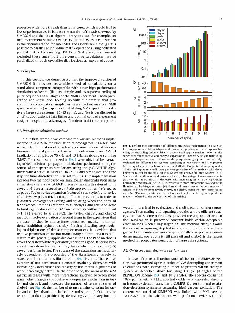
Fig. 1. Performance comparison of different strategies implemented in SIMPSONfor propagator calculation (dsyev and dsyevr: diagonalization based approachesusing corresponding LAPACK drivers; pade – Padé approximation; taylor: Taylorseries expansion; cheby1 and cheby2: expansion in Chebyshev polynomials usingscaling-and-squaring and shift-and-scale pre-processing options, respectively)evaluated for different spin systems consisting of one carbon and 1–9 protons(including all dipole–dipole interactions and 70 kHz CW proton decoupling under15 kHz MAS spinning conditions). (a) Average timing of the methods with dsyevbeing the fastest for the smallest spin system and cheby2 for large systems. (b–d)Statistics of Hamiltonians and series methods. (b) Percentage of non-zero elements(nnz) within the Hamiltonian decreases with increasing system size. (c) Averagenorm of the matrix HDt (Dt = 2 ls) increases with more interactions involved in theHamiltonian for bigger systems. (d) Number of terms needed for convergence ofexpansion series methods taylor, cheby1, and cheby2 using the same color codingas in (a). (For interpretation of the references to color in this figure legend, thereader is referred to the web version of this article.)

5.1. Propagator calculation methods

In our first example we compare the various methods imple-mented in SIMPSON for calculation of propagators. As a test casewe selected simulation of a carbon spectrum influenced by one-to-nine additional protons subjected to continuous wave (CW) rfirradiation of amplitude 70 kHz and 15 kHz magic-angle spinning(MAS). The results summarized in Fig. 1 were obtained by averag-ing of 400 individual propagator calculations performed during thecourse of the spectrum simulations using the c-COMPUTE algo-rithm with a set of 10 REPULSION (a, b), and 8 c angles, the timestep for time discretization was set to 2 ls. Our implementationincludes two methods based on Hamiltonian diagonalization usingeither dsyev or dsyevr LAPACK drivers (henceforth referred to asdsyev and dsyevr, respectively), Padé approximation (referred toas pade), Taylor series expansion (referred to as taylor), and seriesof Chebyshev polynomials taking different precautions in order toguarantee convergence: Scaling-and-squaring when the norm ofHDt exceeds limit of 1 (referred to as cheby1), and shift-and-scaleto limit eigenvalues of the HDt matrix to lay within the interval(�1, 1) (referred to as cheby2). The taylor, cheby1, and cheby2methods involve evaluation of several terms in the expansions thatare accomplished by sparse-times-dense real matrix multiplica-tions. In addition, taylor and cheby1 finish with scaling step involv-ing multiplications of dense complex matrices. It is evident thatrelative performances are not dramatically different and it is diffi-cult to make generally applicable conclusions. The Padé method isnever the fastest while taylor always performs good. It seems ben-eficial to use dsyev for small spin system while for more spins (P6)dsyevr performs better. The success of the expansion methods lar-gely depends on the properties of the Hamiltonian, namely itssparsity and the norm as illustrated in Fig. 1b and c. The relativenumber of non-zero matrix elements markedly decreases withincreasing system dimension making sparse matrix algorithms towork increasingly better. On the other hand, the norm of the HDtmatrix increases with more interactions involved between morespins, which triggers the scaling-and-squaring mechanism in tay-lor and cheby1, and increases the number of terms in series ofcheby2 (see Fig. 1d, the number of terms remains constant for tay-lor and cheby1 thanks to the scaling-and-squaring). One may betempted to fix this problem by decreasing Dt time step but this

would in turn lead to evaluation and multiplication of more prop-agators. Thus, scaling-and-squaring provides a more efficient strat-egy that saves some operations, provided the approximation thatthe Hamiltonian is piecewise constant holds within acceptableerror bounds when using larger Dt. The method cheby2 avoidsthe expensive squaring step but needs more iterations for conver-gence. As this only involves computationally cheap sparse-times-dense matrix operations it still pays off and cheby2 is the fastestmethod for propagator generation of large spin systems.

5.2. CW decoupling: single-core performance

In tests of the overall performance of the current SIMPSON ver-sion, we performed again a series of CW decoupling experimentcalculations with increasing number of protons within the spinsystem as described above but using 168 (a, b) angles of theREPULSION scheme [53] and 10 c angles. The spectra consisting1024 points with a 5 kHz spectral width were generated directlyin frequency domain using the c-COMPUTE algorithm and excita-tion–detection symmetry assuming ideal carbon excitation. Thecurrent version 4 of SIMPSON was linked with MKL version12.1.2.273, and the calculations were performed twice with and

2 4 6 8 1010

−1

100

101

102

103

104

105

Number of spins

Tim

e [s

]

v4 + blockdiag.v4spinevolutionv1

Fig. 2. Computation time of CW decoupling experiment as a function of spin systemsize. The simulations include a single 13C spin connected to 1–9 1H spins performedusing SIMPSON version 1 (v1, black, open circles), SPINEVOLUTION [14] version3.4.5 (blue, open triangles), the current version of SIMPSON without making use ofblock diagonalization (v4, red, open squares), and with taking advantage of blockdiagonalization (v4+blockdiag., red, filled circles), In all cases the computation wasperformed on a single core of Intel Xeon processor computer running CentOS 6.3linux system. (For interpretation of the references to color in this figure legend, thereader is referred to the web version of this article.)

86 Z. Tošner et al. / Journal of Magnetic Resonance 246 (2014) 79–93

without Hamiltonian block diagonalization with respect to the 13Cspin (it splits the Hamiltonian into two blocks of identical dimen-sion), and are referred to as v4+blockdiag and v4 in Fig. 2 (bothusing cheby2 propagator method). The original SIMPSON version1 does not allow for frequency domain calculations nor arbitraryspectral widths and an ‘‘as-close-as-possible’’ setup was used forillustration purposes (referred to as v1). Equivalent calculationswere also done with SPINEVOLUTION package of version 3.4.5.All the simulations were performed on a single core (i.e., with noparallelization on any level) of Intel Xeon processor computer run-ning CentOS 6.3 linux operating system.

The wall-clock times for the benchmark calculations are pre-sented in Fig. 2. It documents dramatic speed improvement (sev-eral orders of magnitude) of the current version with respect tothe original releases of SIMPSON, and a performance similar toSPINEVOLUTION. Importantly, when adding more spins to the sim-ulation, both programs scale essentially identically, with SIMPSONbeing somewhat slower for larger spin systems. For small spin sys-tems (up to �5 spins) the differences in performance are marginaland calculations are finished within a second. For larger spin sys-tems, the time spent on matrix manipulations strongly exceedsany other operations, and the simulation time is largely not beaffected by startup and other operations requiring small amountsof time. It is claimed that the efficiency of SPINEVOLUTION isderived from approximating the propagators by the Chebyshevseries, which scale better with matrix size than diagonalizationmethods, thanks to exploring the Hamiltonian sparsity. One caninspect the time complexity of the overall calculations on thematrix dimension n in the form t = nk. Doing this, we find an expo-nent k = 2.7 (both for SIMPSON and SPINEVOLUTION), which isindeed smaller than 3 predicted for diagonalization of dense matri-ces. We note that all of these comparisons are guiding but may besubject to variations across computer architectures and dependingon the type of simulation.

5.3. Heteronuclear decoupling methods: novel acquisition commands

In solid-state NMR spectroscopy of organic and biological com-pounds heteronuclear decoupling is a major issue, which overmany years have attracted considerable attention as a means toimprove spectra resolution. This has led to the development of

many pulse sequences including TPPM [90], SPINAL [91], XiX[92], PISSARRO [93], symmetry-based CN [94] and RN [95]sequences as well as advanced theoretical methods for under-standing of their performance and systematic development of suchexperiments [96–98].

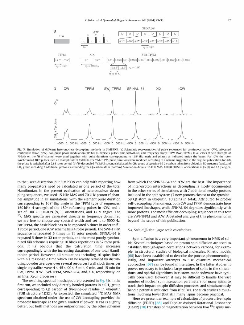
As the effect of heteronuclear decoupling typically dependshighly on the spin system, involving effects from both heteronu-clear and homonuclear interactions as well as the chemical shiftparameters, evaluation of decoupling performance eventually hasto rely on experimental comparison, and with the developmentof efficient numerical simulation programs also on numerical sim-ulations. We here take the latter approach and demonstrate howefficient calculation of decoupling in large spin systems by SIMP-SON may add to the discussion of relative performance of differentdecoupling methods. From the extensive list of heteronucleardecoupling sequences, we have for the purpose of demonstrationselected continuous wave (CW) irradiation, two-pulse phase mod-ulation (TPPM) [90], frequency swept TPPM (SWf-TPPM) [99],SPINAL-64 [91], XiX [92], and refocused continuous wave (rCW)[100] decoupling methods. The corresponding pulse sequences,summarized in Fig. 3a, differ in complexity, and some of themare difficult to implement in current NMR simulation software,particularly when addressing synchronization with MAS anddetection dwell time periods.

With the new acq_block command, SIMPSON now offers aparticularly simple way of implementing rf irradiation duringacquisition, which is basically identical to typical implementationson real NMR spectrometers. Pulse sequence events are specified asthey come in time, without a need to chop them into blocks ofdwell time, as it was necessary in previous versions of SIMPSON.For example, XiX decoupling is coded as follows,

acq_block {

pulse $par(tp) $par(rf) x 0 0

pulse $par(tp) $par(rf) –x 0 0

}

where par(tp) defines duration of the pulse, i.e. 2.85 times a rotorperiod. SIMPSON itself then checks for periodicity and synchroniza-tion, and repeats the sequence as necessary. The FID/spectrum iscalculated using the COMPUTE algorithm in time/frequencydomain. The algorithm specific parameter defining the numberof propagation steps taken within a cycle can be defined inpar(points_per_cycle) and is automatically taken into accountin splitting the sequence into smaller time intervals. We note thatany commands dedicated for pulse sequence section of the SIMP-SON input file (pulse, pulseid, delay, offset, pulse_shaped,prop) can be used within the acq_block command. As a secondexample demonstrating the versatility of the programming, theSPINAL-64 scheme can be nicely implemented using a shaped pulse,

acq_block {pulse_shaped $par(tp) $spinal64shape nothing}

with all rf amplitudes and phases defined in the shape variablespinal64shape (the keyword nothing is used to define there isno rf irradiation on the second channel – 13C). The shape filemerely includes a list of pulse amplitudes and phases as describedpreviously in Ref. [16].

The computation time depends critically on pulse sequenceevent synchronization. While for CW experiment one can use effi-cient c-COMPUTE algorithm, it is not directly possible for the othercases (although we realize one can adjust the spectral width andaveraging over c-angles for TPPM in order to meet restrictions onperiodicity of rf Hamiltonian). Proper synchronization is still left

a

b

Fig. 3. Simulation of different heteronuclear decoupling methods in SIMPSON. (a) Schematic representation of pulse sequences for continuous wave (CW), refocusedcontinuous wave (rCW), two-pulse phase modulation (TPPM), x-inverse x pulse (XiX), SPINAL-64, and frequency swept TPPM (SWf-TPPM). In all cases rf field strength of70 kHz on the 1H rf channel were used together with pulse durations corresponding to 168� flip angle and phases as indicated inside the boxes. For rCW the rotorsynchronized 180� pulses used an rf amplitude of 150 kHz. For SWf-TPPM, pulse durations were modified according to a scheme suggested in the original publication, for XiXthe phase is switched after 2.85 rotor period. (b) 1H-decoupled 13C MAS spectra calculated for CH2 group of tyrosine-59 Cb carbon taken from ubiquitin 3D structure (top), andCH2 group including 7 additional protons surrounding the Cb carbon atom (bottom). Simulation details: 15 kHz MAS, 100 REPULSION orientations of (a, b) and 12 c angles.

Z. Tošner et al. / Journal of Magnetic Resonance 246 (2014) 79–93 87

to the user’s discretion, but SIMPSON can help with reporting howmany propagators need be calculated in one period of the totalHamiltonian. In the present evaluation of heteronuclear decou-pling sequences, we used 15 kHz MAS and 70 kHz proton rf chan-nel amplitude in all simulations, with the element pulse durationcorresponding to 168� flip angle in the TPPM type of sequences,150 kHz rf strength of the 180� refocusing pulses in rCW, and aset of 100 REPULSION [a, b] orientations, and 12 c angles. The13C MAS spectra are generated directly in frequency domain sowe are free to choose any spectral width and set it to 5000 Hz.For TPPM, the basic block has to be repeated 5 times in order to fill1 rotor period, one rCW scheme fills 4 rotor periods, the SWf-TPPMsequence is repeated 5 times in 11 rotor periods, SPINAL-64 isrepeated 5 times in 32 rotor periods, and the most poorly synchro-nized XiX scheme is requiring 10 block repetitions in 57 rotor peri-ods. It is obvious that the calculation time increasescorrespondingly with the increasing durations of one total Hamil-tonian period. However, all simulations including 10 spins finishwithin a reasonable time which can be readily reduced by distrib-uting powder averages over several resources (wall clock times persingle crystallite were 4 s, 45 s, 90 s, 5 min, 9 min, and 15 min forCW, TPPM, rCW, SWf-TPPM, SPINAL-64, and XiX, respectively, onan Intel Xeon processor).

The resulting spectral lineshapes are presented in Fig. 3b. In thefirst run, we included only directly bonded protons in a CH2 groupcorresponding to Cb carbon of tyrosine-59 residue in ubiquitin(PDB structure 1D3Z). As expected, the simulated 13C MAS NMRspectrum obtained under the use of CW decoupling provides thebroadest lineshape at the given limited rf power. TPPM is slightlybetter, but both methods are outperformed by the other schemes

from which the SPINAL-64 and rCW are the best. The importanceof inter-proton interactions in decoupling is nicely documentedin the other series of simulations with 7 additional nearby protonsincluded in the spin system (7 new protons closest to the tyrosine-59 Cb atom in ubiquitin, 10 spins in total). Attributed to protonself-decoupling phenomena, both CW and TPPM demonstrate hereimproved lineshapes, while SPINAL-64 degrades significantly withmore protons. The most efficient decoupling sequences in this testare SWf-TPPM and rCW. A detailed analysis of this phenomenon isbeyond the scope of this publication.

5.4. Spin diffusion: large scale calculations

Spin diffusion is a very important phenomenon in NMR of sol-ids. Several techniques based on proton spin diffusion are used toestablish through-space correlations between carbons, for exam-ple, in structural studies of biological molecules. Kinetic models[66] have been established to describe the process phenomenolog-ically, and important attempts to use quantum mechanicalapproaches [67] can be found in literature. In the latter studies, itproves necessary to include a large number of spins in the simula-tions, and special algorithms in custom-made software have typi-cally been used. However, it may be difficult to handle the vastnumber of nuclear spin interaction parameters for many spins, totrack their impact on spin diffusion processes, and simultaneouslyhandle potential influence from rf pulses. For such studies simula-tions involving fewer (but still many) spins become practical.

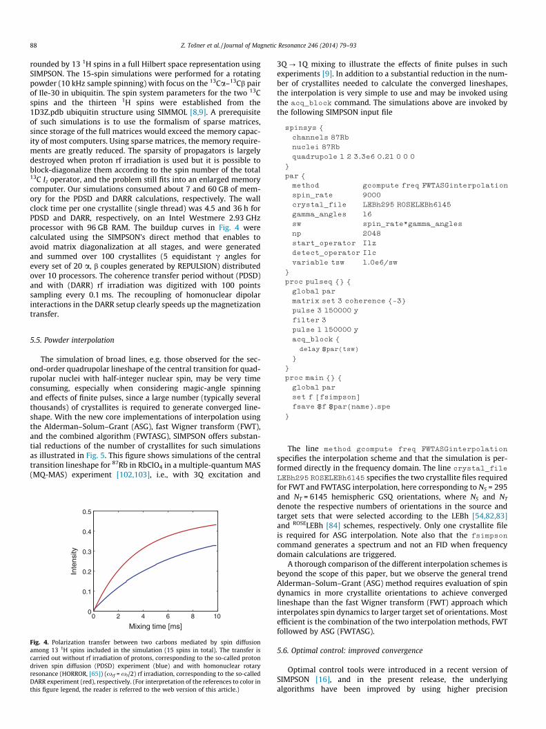
Here we present an example of calculation of proton driven spindiffusion (PDSD) [68] and Dipolar Assisted Rotational Resonance(DARR) [70] transfers of magnetization between two 13C spins sur-

88 Z. Tošner et al. / Journal of Magnetic Resonance 246 (2014) 79–93

rounded by 13 1H spins in a full Hilbert space representation usingSIMPSON. The 15-spin simulations were performed for a rotatingpowder (10 kHz sample spinning) with focus on the 13Ca–13Cb pairof Ile-30 in ubiquitin. The spin system parameters for the two 13Cspins and the thirteen 1H spins were established from the1D3Z.pdb ubiquitin structure using SIMMOL [8,9]. A prerequisiteof such simulations is to use the formalism of sparse matrices,since storage of the full matrices would exceed the memory capac-ity of most computers. Using sparse matrices, the memory require-ments are greatly reduced. The sparsity of propagators is largelydestroyed when proton rf irradiation is used but it is possible toblock-diagonalize them according to the spin number of the total13C Iz operator, and the problem still fits into an enlarged memorycomputer. Our simulations consumed about 7 and 60 GB of mem-ory for the PDSD and DARR calculations, respectively. The wallclock time per one crystallite (single thread) was 4.5 and 36 h forPDSD and DARR, respectively, on an Intel Westmere 2.93 GHzprocessor with 96 GB RAM. The buildup curves in Fig. 4 werecalculated using the SIMPSON’s direct method that enables toavoid matrix diagonalization at all stages, and were generatedand summed over 100 crystallites (5 equidistant c angles forevery set of 20 a, b couples generated by REPULSION) distributedover 10 processors. The coherence transfer period without (PDSD)and with (DARR) rf irradiation was digitized with 100 pointssampling every 0.1 ms. The recoupling of homonuclear dipolarinteractions in the DARR setup clearly speeds up the magnetizationtransfer.

5.5. Powder interpolation

The simulation of broad lines, e.g. those observed for the sec-ond-order quadrupolar lineshape of the central transition for quad-rupolar nuclei with half-integer nuclear spin, may be very timeconsuming, especially when considering magic-angle spinningand effects of finite pulses, since a large number (typically severalthousands) of crystallites is required to generate converged line-shape. With the new core implementations of interpolation usingthe Alderman–Solum–Grant (ASG), fast Wigner transform (FWT),and the combined algorithm (FWTASG), SIMPSON offers substan-tial reductions of the number of crystallites for such simulationsas illustrated in Fig. 5. This figure shows simulations of the centraltransition lineshape for 87Rb in RbClO4 in a multiple-quantum MAS(MQ-MAS) experiment [102,103], i.e., with 3Q excitation and

0 2 4 6 8 100

0.1

0.2

0.3

0.4

0.5

Mixing time [ms]

Inte

nsity

Fig. 4. Polarization transfer between two carbons mediated by spin diffusionamong 13 1H spins included in the simulation (15 spins in total). The transfer iscarried out without rf irradiation of protons, corresponding to the so-called protondriven spin diffusion (PDSD) experiment (blue) and with homonuclear rotaryresonance (HORROR, [65]) (xrf = xr/2) rf irradiation, corresponding to the so-calledDARR experiment (red), respectively. (For interpretation of the references to color inthis figure legend, the reader is referred to the web version of this article.)

3Q ? 1Q mixing to illustrate the effects of finite pulses in suchexperiments [9]. In addition to a substantial reduction in the num-ber of crystallites needed to calculate the converged lineshapes,the interpolation is very simple to use and may be invoked usingthe acq_block command. The simulations above are invoked bythe following SIMPSON input file

spinsys {

channels 87Rb

nuclei 87Rb

quadrupole 1 2 3.3e6 0.21 0 0 0

}

par {

method

gcompute freq FWTASGinterpolation

spin_rate

9000

crystal_file

LEBh295 ROSELEBh6145

gamma_angles

16

sw

spin_rate*gamma_angles

np

2048

start_operator

I1z

detect_operator

I1c

variable tsw

1.0e6/sw

}

proc pulseq {} {

global par

matrix set 3 coherence {-3}

pulse 3 150000 y

filter 3

pulse 1 150000 y

acq_block {

delay $par(tsw)

}

}

proc main {} {

global par

set f [fsimpson]

fsave $f $par(name).spe

}

The line method gcompute freq FWTASGinterpolation

specifies the interpolation scheme and that the simulation is per-formed directly in the frequency domain. The line crystal_file

LEBh295 ROSELEBh6145 specifies the two crystallite files requiredfor FWT and FWTASG interpolation, here corresponding to NS = 295and NT = 6145 hemispheric GSQ orientations, where NS and NT

denote the respective numbers of orientations in the source andtarget sets that were selected according to the LEBh [54,82,83]and ROSELEBh [84] schemes, respectively. Only one crystallite fileis required for ASG interpolation. Note also that the fsimpson

command generates a spectrum and not an FID when frequencydomain calculations are triggered.

A thorough comparison of the different interpolation schemes isbeyond the scope of this paper, but we observe the general trendAlderman–Solum–Grant (ASG) method requires evaluation of spindynamics in more crystallite orientations to achieve convergedlineshape than the fast Wigner transform (FWT) approach whichinterpolates spin dynamics to larger target set of orientations. Mostefficient is the combination of the two interpolation methods, FWTfollowed by ASG (FWTASG).

5.6. Optimal control: improved convergence

Optimal control tools were introduced in a recent version ofSIMPSON [16], and in the present release, the underlyingalgorithms have been improved by using higher precision

−6−40 −22

NS = 6145

NS = 1177

NS = 295

NS = 55

NS = 2905

NS = 1177

NS = 295

NS = 55

NT = 55297

NS = 2905

NS = 1177

NS = 295

NS = 55

NT = 6145

ν/kHz−6−40 −22

ν/kHz−6−40 −22

ν/kHz

cba

Fig. 5. Demonstration of SIMPSON procedures for powder interpolation used to assess lineshape distortions in MQ-MAS experiment. Short 150 kHz rf pulses were used toexcite triple-quantum coherences and to convert it into single-quantum central transition coherence of 87Rb (I = 3/2, CQ = 3.3 MHz, g = 0.21) [89,101] at 9.4 T magnetic fieldstrength and 9 kHz MAS. The columns correspond to the three interpolation methods: (a) Alderman–Solum–Grant (ASG), (b) Fast Wigner transformation (FWT), (c) Thecombination of FWT and ASG (FWTASG). Rows correspond to simulations using different numbers of crystallites. The top row corresponds to fully converged spectra.

Z. Tošner et al. / Journal of Magnetic Resonance 246 (2014) 79–93 89

gradients and quasi-Newton optimization. It was noted in Ref. [61]that the gradient update originally proposed in the original GRAPEalgorithm of Khaneja et al. [35] represents only a first-orderapproximation and that using it in more elaborate optimizationalgorithms (that make use of second derivatives and are expectedto converge faster) does not provide satisfactory results. It istherefore essential to use higher precision gradients of an OCpropagator with respect to rf amplitudes in order to speed upconvergence. Such calculation is controlled by parameterpar(oc_grad_level) which corresponds to the order of thegradient approximation. Equipped with this, the user canchoose between original conjugated gradients (CG) andL-BFGS algorithms for optimization through definition ofpar(oc_method) to CG and L-BFGS, respectively. Both methodshave many additional parameters that are described at our websitehttp://www.nmr.au.dk.

For the purpose of demonstration, we repeat the OC-based2H–13C cross-polarization published recently [78]. We assume 2His in spin state corresponding to Ix and want to find a pulsesequence which maximizes the transfer to the carbon Ix state, withefficiency described by a function U (U = 1 for 100% transfer). Weset the duration of the pulse to 800 ls and divide it into 1 ls longelements, resulting altogether to 3200 optimization variables (800for each x and y rf components on two channels). Further settingsinclude 20 kHz MAS and averaging over 20 (a, b) REPULSION orien-tations and 8 c angles. The optimizations were done separately fororiginal CG with first and second order precision gradient (referredto as CG1 and CG2, respectively), and for L-BFGS using secondorder precision gradient. As can be seen from Fig. 6a, CG2 indeedprovides solutions with higher transfer efficiency at the same iter-ation compared to CG1, and L-BFGS is still even better. So, not onlydo we gain about 10% in transfer efficiency, the calculation time-savings are also evident. The plot of U against CPU time presentedin Fig. 6b shows dramatic reduction for the L-BFGS method that notonly provides a better solution but also finishes much faster. Thefinal rf sequence depicted in Fig. 6c and d provides 98.7% transferefficiency at the given conditions and clearly possesses featuressynchronized with sample rotation (Fourier transform analysis

reveals distinct peaks at multiples of MAS frequency, data notshown).

5.7. Spectral fitting: linking with external libraries

To enable spectral fitting in SIMPSON, we have developed a newTcl optimization package based on the SIMPLEX optimization rou-tines implemented in the package optimization1.0, which is part ofthe molecular visualization program VMD [104]. This package,called opt, replaces the SIMPSON implementation of MINUIT[105]. The package is written in Tcl to ensure smooth installationacross all platforms and is loaded through the Tcl interface ofSIMPSON as follows

lappend::auto_path /path/to/opt/directory

package require opt

The first line points to the installation path of the opt directory,whereas the second line loads the package into the Tcl interpreter.Since the main time consuming step in the computation is by farthe generation of a trial FID/spectrum, there is no significant per-formance disadvantage of using Tcl scripts.

To illustrate the capabilities of opt, Fig. 7a shows the experi-mental 15N spectrum of alamethicin with 15N label on Aib8 in ori-ented lipid bilayers, recorded using 1H FSLG decoupling to yield aduplet due to the 1H–15N dipole–dipole coupling between theamide proton and nitrogen. This spectrum has been reported else-where [106,107], and represents an obvious case for SIMPSON,since simulation of the spectrum requires inclusion of mosaicspread (non-uniform powder averaging) and effects from finitepulses. To simulate the spectrum, we first generate a newcrystallite file containing a Gaussian distribution of crystallitesaround the North pole to represent the mosaic spread, whichmay be loaded into SIMPSON using the standard definition ofpar(crystal_file). We may also use the possibility of usingcrystallite interpolation, in which case we should also generate acrystallite triangle file describing the vertices of the triangles.

0 200 400 600 800−100

−50

0

50

100

Time [μs]

ωy/2

π [k

Hz]

c

a

−50

0

50

100

ωx/2

π [k

Hz]

0 200 400 600 800−100

−50

0

50

100

Time [μs]

ωy/2

π [k

Hz]

d

b

−100

−50

0

50

100

ωx/2

π [k

Hz]

0 100 200 3000

0.2

0.4

0.6

0.8

1

CPU time [min]

Φ

CG 1CG 2L−BFGS

0 200 400 6000

0.2

0.4

0.6

0.8

1

Number of iterations

ΦCG 1CG 2L−BFGS

Fig. 6. Demonstration of SIMPSON optimal control tools in pulse sequence design for polarization transfer from 2H to directly attached 13C mediated by dipole–dipoleinteraction. (a) Transfer efficiency vs. number of iterations for the original conjugated gradient method with first-order approximation of the gradient (CG1, red), second-order approximation (CG2, green), and the limiter memory BFGS algorithm (L-BFGS, blue). (b) Transfer efficiency as a function of CPU time. (c and d) Resulting rf amplitudes(top: x-phase, bottom: y-phase) for the 2H (c) and 13C (d) channels. (For interpretation of the references to color in this figure legend, the reader is referred to the web versionof this article.)

90 Z. Tošner et al. / Journal of Magnetic Resonance 246 (2014) 79–93

The FSLG-decoupling pulse sequence is easily implemented usingthe new acq_block command

proc pulseq {} {

global par

acq_block {

offset 0 $par(offH)

pulse $par(tsw2) 0 x $par(rfH) x

offset 0 [expr -$par(offH)]

pulse $par(tsw2) 0 x $par(rfH) -x

}

}

where the pulse length ($par(tsw2)), carrier offset ($par(offH))and rf field strength ($par(rfH)) have been calculated previouslyto match the FSLG condition.

Since the isotropic chemical shift is known from other experi-ments [108], we only need to optimize the anisotropic chemicalshift, the 1H–15N dipole–dipole coupling, and the degree of mosaicspread. To convincingly model the spectrum, we will also includethe linebroadening as a parameter in the optimization. Theseparameters are defined as optimization targets by the followingcommands

opt::newpar csa 6000 50

opt::newpar dip 7000 50

opt::newpar dist 15 1

opt::newpar lb 500 50

opt::function rms

For each parameter is specified the name, the initial value, andthe initial step size. The current value for these parameters areaccessed through the Tcl variables $opt::csa, etc. The last line

specifies that the optimization routine should optimize theseparameters using the return value of the Tcl procedure rms. Inthe present case, this routine contains the elements

proc rms {} {

global par

generate_mosaic_spread $opt::dist

set f [fsimpson [listn[list shift_1_aniso $opt::csa]n[list dipole_1_2_aniso $opt::dip]n

]]

...

faddlb $f $opt::lb 1

...

set rms [frms $f $par(f) -re]

...

return $rms

}

The package opt provides a number of commands for control-ling the optimization, fixing, releasing and scanning parameters,and for calculation of 95% confidence intervals, e.g.,

opt::scan csa

opt::minimize

opt::fix bdist

opt::release bdist

set c95 [opt::confidence csa]

The possibility of calculating 95% confidence intervals is exempli-fied in Fig. 7b. To calculate the confidence interval, the targetparameter is fixed at different values around its optimum value,and for each of these values, all other parameters are optimized.

18

19

20

21

6000 6200 6400

18

19

20

21

7200 7400 7600

18

19

20

21

1000 1200 1400 1600

18

19

20

21

14 16 18 20

7014021028015N shift (ppm)

RMS

(a.u

.)RM

S (a

.u.)

15N CSA (Hz)

Line broadening (Hz)

1H-15N Dip. coupl. (Hz)

Mosaic spread (deg)

a

b

Fig. 7. (a) Experimental (bottom) and simulated (top) 15N spectra of alamethicinwith 15N labelling of Aib8 in oriented lipid bilayers. The spectrum is recorded using1H FSLG decoupling resulting in the presence of a duplet due to the 1H–15N dipole–dipole coupling between the amide proton and nitrogen. The asymmetry of theduplet is due to mosaic spread [106,107]. (b) Calculations of 95% confidenceintervals for the four parameters optimized. The solid lines represent the parabolicfit to the points.

Z. Tošner et al. / Journal of Magnetic Resonance 246 (2014) 79–93 91

The optimum RMS value for the different values of the targetparameter should represent a parabola

RMSðxÞ ¼ aðx� bÞ2 þ c

and the 95% confidence interval, obtained as C95 ¼ 2=ffiffiffiap

, representsthe statistical uncertainty of a parameter. In the present optimiza-tion, the resulting parameters and 95% confidence intervals are

csa = 6161 ± 204 Hz

dip = 7330 ± 332 Hz

bdist = 17 ± 3 deg

lb = 1155 ± 397 Hz

The opt package including detailed documentation is availablefor download from our web site http://www.nmr.au.dk.

6. Conclusion

Since its release in 2000, the open source software packageSIMPSON for numerical simulations of solid-state NMR

experiments has become very popular within the NMR commu-nity. In this paper, we have presented its improved version withmany new features, performance matching other comparable soft-ware packages, and optimized for parallel applications. Among itsmajor advantages are flexible and yet simple user interface basedon the Tcl scripting language, allowing for simulation of essentiallyany NMR experiment. The user has full control over used numeri-cal algorithms and parallelization procedures, as well as core linearalgebra routines. By these means the program can be optimized fora given computer architecture. We have demonstrated its usage forsimulating NMR response in relatively large spin systems andunder a distribution of experimental conditions. It is also worthto mention that SIMPSON includes optimal control tools enablingautomatic computer design of new NMR experiments that stronglybenefits from new features introduced in this version.

The SIMPSON software is available for download from our website, together with input files of all examples presented here. Inter-ested readers are also encouraged to join our effort and contributeto the software through the open project philosophy.

Acknowledgments

We acknowledge support from the Danish National ResearchFoundation (DNRF59), the Danish Center for Scientific Computing,Lundbeckfonden, the Faculty of Sciences at Stockholm University,the European Commission under the Seventh Framework Pro-gramme (FP7) contract Bio-NMR 261863.

References

[1] A.C. Sivertsen, M. Bjerring, C.T. Kehlet, T. Vosegaard, N.C. Nielsen, Numericalsimulations in biological solid-state NMR spectroscopy, Annu. Rev. NMR 54(2005) 243–293.

[2] N.C. Nielsen, Computational aspects of biological solid-state NMRspectroscopy, in: A. Ramamoorthy (Ed.), NMR Spectroscopy of BiologicalSolids, CRC/Taylor & Francis, 2006, pp. 261–304.

[3] F.S. Debouregas, J.S. Waugh, Antiope, a program for computer experiments onspin dynamics, J. Magn. Reson. 96 (1992) 280–289.

[4] S.A. Smith, T.O. Levante, B.H. Meier, R.R. Ernst, Computer-simulations inmagnetic-resonance – an object-oriented programming approach, J. Magn.Reson. A 106 (1994) 75–105.

[5] H. Bildsøe, STARS User’s Guide, Spectrum Analysis for Rotating Solids, Publ.No. 87-195233-00, Rev. A0296, Varian Associates Inc., Palo Alto, 1996.

[6] J. Skibsted, N.C. Nielsen, H. Bildsoe, H.J. Jakobsen, Satellite transitions in MasNMR-spectra of quadrupolar nuclei, J. Magn. Reson. 95 (1991) 88–117.

[7] M. Bak, J.T. Rasmussen, N.C. Nielsen, SIMPSON: a general simulation programfor solid-state NMR spectroscopy, J. Magn. Reson. 147 (2000) 296–330.

[8] M. Bak, R. Schultz, T. Vosegaard, N.C. Nielsen, Specification and visualizationof anisotropic interaction tensors in polypeptides and numerical simulationsin biological solid-state NMR, J. Magn. Reson. 154 (2002) 28–45.

[9] T. Vosegaard, A. Malmendal, N.C. Nielsen, The flexibility of SIMPSON andSIMMOL for numerical simulations in solid- and liquid-state NMRspectroscopy, Monatsh. Chem. 133 (2002) 1555–1574.

[10] P. Hodgkinson, PNMRsim: A General Simulation Program for Large Problemsin Solid-state NMR, Durham University, 2000.

[11] D. Massiot, F. Fayon, M. Capron, I. King, S. Le Calvé, B. Alonso, J.-O. Durand, B.Bujoli, Z. Gan, G. Hoatson, Modelling one- and two-dimensional solid-stateNMR spectra, Magn. Reson. Chem. 40 (2002) 70–76.

[12] W.B. Blanton, BlochLib: a fast NMR C++ tool kit, J. Magn. Reson. 162 (2003)269–283.

[13] A. Jerschow, MathNMR: spin and spatial tensor manipulations inMathematica, J. Magn. Reson. 176 (2005) 7–14.

[14] M. Veshtort, R.G. Griffin, SPINEVOLUTION: a powerful tool for the simulationof solid and liquid state NMR experiments, J. Magn. Reson. 178 (2006) 248–282.

[15] J.D. van Beek, MatNMR: a flexible toolbox for processing, analyzing andvisualizing magnetic resonance data in Matlab((R)), J. Magn. Reson. 187(2007) 19–26.

[16] Z. Tosner, T. Vosegaard, C. Kehlet, N. Khaneja, S.J. Glaser, N.C. Nielsen, Optimalcontrol in NMR spectroscopy: numerical implementation in SIMPSON, J.Magn. Reson. 197 (2009) 120–134.

[17] H.J. Hogben, M. Krzystyniak, G.T.P. Charnock, P.J. Hore, I. Kuprov, Spinach – asoftware library for simulation of spin dynamics in large spin systems, J.Magn. Reson. 208 (2011) 179–194.

[18] M.H. Levitt, SpinDynamica, Southampton, 2011.

92 Z. Tošner et al. / Journal of Magnetic Resonance 246 (2014) 79–93

[19] M. Edén, Y.K. Lee, M.H. Levitt, Efficient simulation of periodic problems inNMR. Application to decoupling and rotational resonance, J. Magn. Reson. A120 (1996) 56–71.

[20] T. Charpentier, C. Fermon, J. Virlet, Efficient time propagation technique forMAS NMR simulation: application to quadrupolar nuclei, J. Magn. Reson. 132(1998) 181–190.

[21] M. Hohwy, H. Bildsoe, H.J. Jakobsen, N.C. Nielsen, Efficient spectralsimulations in NMR of rotating solids. The gamma-COMPUTE algorithm, J.Magn. Reson. 136 (1999) 6–14.

[22] P. Hodgkinson, L. Emsley, Numerical simulation of solid-state NMRexperiments, Prog. Nucl. Magn. Reson. 36 (2000) 201–239.

[23] M. Edén, Computer simulations in solid-state NMR. I. Spin dynamics theory,Concepts Magn. Reson. 17A (2003) 117–154.

[24] M. Edén, Computer simulations in solid-state NMR. II. Implementations forstatic and rotating samples, Concepts Magn. Reson. 18A (2003) 1–23.

[25] M. Edén, Computer simulations in solid-state NMR. III. Powder averaging,Concepts Magn. Reson. 18A (2003) 24–55.

[26] N.C. Nielsen, T. Vosegaard, A. Malmendal, Analytical and numerical tools forexperiment design in solid-state NMR spectroscopy, in: G.A. Webb (Ed.),Modern Magnetic Resonance. Applications in Chemistry, Biological andMarine Sciences, Springer, 2006, pp. 679–687.

[27] I. Kuprov, N. Wagner-Rundell, P.J. Hore, Polynomially scaling spin dynamicssimulation algorithm based on adaptive state-space restriction, J. Magn.Reson. 189 (2007) 241–250.

[28] I. Kuprov, Polynomially scaling spin dynamics II: further state-spacecompression using Krylov subspace techniques and zero track elimination,J. Magn. Reson. 195 (2008) 45–51.

[29] L. Emsley, M.C. Butler, J.N. Dumez, Dynamics of large nuclear-spin systemsfrom low-order correlations in Liouville space, Chem. Phys. Lett. 477 (2009)377–381.

[30] H.J. Hogben, P.J. Hore, I. Kuprov, Strategies for state space restriction indensely coupled spin systems with applications to spin chemistry, J. Chem.Phys. 132 (2010).

[31] L. Emsley, J.N. Dumez, M.C. Butler, Numerical simulation of free evolution insolid-state nuclear magnetic resonance using low-order correlations inLiouville space, J. Chem. Phys. 133 (2010).

[32] T. Vosegaard, Challenges in numerical simulations of solid-state NMRexperiments: spin exchange pulse sequences, Solid State Nucl. Magn.Reson. 38 (2010) 77–83.

[33] L.S. Pontryagin, The Mathematical Theory of Optimal Processes, IntersciencePublishers, New York, 1962.

[34] A.E. Bryson, Y.-C. Ho, Applied Optimal Control: Optimization, Estimation, andControl, Rev. printing. ed., Hemisphere Pub. Corp.; distributed by HalstedPress, Washington, New York, 1975.

[35] N. Khaneja, T. Reiss, C. Kehlet, T. Schulte-Herbruggen, S.J. Glaser, Optimalcontrol of coupled spin dynamics: design of NMR pulse sequences by gradientascent algorithms, J. Magn. Reson. 172 (2005) 296–305.

[36] C.T. Kehlet, A.C. Sivertsen, M. Bjerring, T.O. Reiss, N. Khaneja, S.J. Glaser, N.C.Nielsen, Improving solid-state NMR dipolar recoupling by optimal control, J.Am. Chem. Soc. 126 (2004) 10202–10203.

[37] I.I. Maximov, Z. Tosner, N.C. Nielsen, Optimal control design of NMR anddynamic nuclear polarization experiments using monotonically convergentalgorithms, J. Chem. Phys. 128 (2008). 184505-184501-184505-184514.

[38] I.I. Maximov, J. Salomon, G. Turinici, N.C. Nielsen, A smoothing monotonicconvergent optimal control algorithm for nuclear magnetic resonance pulsesequence design, J. Chem. Phys. 132 (2010) 084107.

[39] T. Vosegaard, C. Kehlet, N. Khaneja, S.J. Glaser, N.C. Nielsen, Improvedexcitation schemes for multiple-quantum magic-angle spinning forquadrupolar nuclei designed using optimal control theory, J. Am. Chem.Soc. 127 (2005) 13768–13769.

[40] Z. Tosner, S.J. Glaser, N. Khaneja, N.C. Nielsen, Effective Hamiltonians byoptimal control: solid-state NMR double-quantum planar and isotropicdipolar recoupling, J. Chem. Phys. 125 (2006) 184502.

[41] C. Kehlet, M. Bjerring, A.C. Sivertsen, T. Kristensen, J.J. Enghild, S.J. Glaser, N.Khaneja, N.C. Nielsen, Optimal control based NCO and NCA experiments forspectral assignment in biological solid-state NMR spectroscopy, J. Magn.Reson. 188 (2007) 216–230.

[42] A.B. Nielsen, M. Bjerring, J.T. Nielsen, N.C. Nielsen, Symmetry-based dipolarrecoupling by optimal control: band-selective experiments for assignment ofsolid-state NMR spectra of proteins, J. Chem. Phys. 131 (2009) 025101.

[43] N.C. Nielsen, C. Kehlet, S.J. Glaser, N. Khaneja, Optimal control methods inNMR spectroscopy, in: R.K. Harris, R.E. Wasylishen (Eds.), Encyclopedia ofMagnetic Resonance, John Wiley & Sons Ltd., Chichester, 2010.

[44] C. Kehlet, J.T. Nielsen, Z. Tosner, N.C. Nielsen, Resolution-enhanced solid-stateNMR 13C–13C correlation spectroscopy by optimal control dipolar-drivenspin-state-selective coherence transfer, J. Phys. Chem. Lett. 2 (2011) 543–547.

[45] N.M. Loening, M. Bjerring, N.C. Nielsen, H. Oschkinat, A comparison of NCOand NCA transfer methods for biological solid-state NMR spectroscopy, J.Magn. Reson. 214 (2012) 81–90.

[46] C. Bretschneider, A. Karabanov, N.C. Nielsen, W. Kockenberger, Conversion ofparahydrogen induced longitudinal two-spin order to evenly distributedsingle spin polarisation by optimal control pulse sequences, J. Chem. Phys.136 (2012) 094201.

[47] M.S. Vinding, Maximov II, Z. Tosner, N.C. Nielsen, Fast numerical design ofspatial-selective rf pulses in MRI using Krotov and quasi-Newton basedoptimal control methods, J. Chem. Phys. 137 (2012) 054203.

[48] C. Laustsen, S. Bowen, M.S. Vinding, N.C. Nielsen, J.H. Ardenkjaer-Larsen,Storage of magnetization as singlet order by optimal control designed pulses,Magn. Reson. Med. 71 (2014) 921–926.

[49] M.S. Vinding, C. Laustsen, Maximov II, L.V. Sogaard, J.H. Ardenkjaer-Larsen,N.C. Nielsen, Dynamic nuclear polarization and optimal control spatial-selective C-13 MRI and MRS, J. Magn. Reson. 227 (2013) 57–61.

[50] S.K. Zaremba, Good lattice points, discrepancy, and numerical integration,Ann. Mat. Pura Appl. 73 (1966) 293.

[51] H. Conroy, Molecular Schrodinger equation. 8. A new method for evaluationof multidimensional integrals, J. Chem. Phys. 47 (1967) 5307.

[52] V.B. Cheng, Investigations of a nonrandom numerical-method formultidimensional integration, J. Chem. Phys. 59 (1973) 3992–3999.

[53] M. Bak, N.C. Nielsen, REPULSION, a novel approach to efficient powderaveraging in solid-state NMR, J. Magn. Reson. 125 (1997) 132–139.

[54] M. Edén, M.H. Levitt, Computation of orientational averages in solid-stateNMR by Gaussian spherical quadrature, J. Magn. Reson. 132 (1998) 220–239.

[55] U. Haeberlen, J.S. Waugh, Coherent averaging effects in magnetic resonance,Phys. Rev. 175 (1968) 453.

[56] M. Hohwy, N.C. Nielsen, Systematic design and evaluation of multiple-pulseexperiments in nuclear magnetic resonance spectroscopy using a semi-continuous Baker–Campbell–Hausdorff expansion, J. Chem. Phys. 109 (1998)3780–3791.

[57] T.S. Untidt, N.C. Nielsen, Closed solution to the Baker–Campbell–Hausdorffproblem: exact effective Hamiltonian theory for analysis of nuclear-magnetic-resonance experiments, Phys. Rev. E 65 (2002) 021108.

[58] D. Siminovitch, T. Untidt, N.C. Nielsen, Exact effective Hamiltonian theory. II.Polynomial expansion of matrix functions and entangled unitary exponentialoperators, J. Chem. Phys. 120 (2004) 51–66.

[59] D.W. Alderman, M.S. Solum, D.M. Grant, Methods for analyzing spectroscopicline shapes. NMR solid powder patterns, J. Phys. Chem. 84 (1986) 3717.

[60] B. Stevensson, M. Edén, Interpolation by fast Wigner transform for rapidcalculations of magnetic resonance spectra from powders, J. Chem. Phys. 134(2011) 124104.

[61] P. de Fouquieres, S.G. Schirmer, S.J. Glaser, I. Kuprov, Second order gradientascent pulse engineering, J. Magn. Reson. 212 (2011) 412–417.

[62] J. Nocedal, Updating quasi-Newton matrices with limited storage, Math.Comput. 35 (1980) 773–782.

[63] S. Blackford, J. Demmel, J. Dongarra, I. Duff, S. Hammarling, G. Henry, M.Heroux, L. Kaufman, A. Lumsdaine, A. Petitet, R. Pozo, K. Remington, R.C.Whaley, An updated set of Basic Linear Algebra Subprograms (BLAS), ACMTrans. Math. Softw. 28 (2002) 135–151.

[64] E. Anderson, Z. Bai, C. Bischof, S. Blackford, J. Demmel, J. Dongarra, J. Du Croz,A. Greenbaum, S. Hammarling, A. McKenney, D. Sorensen, LAPACK Users’Guide, third ed., Society for Industrial and Applied Mathematics, Philadelphia,PA, 1999.

[65] N.C. Nielsen, H. Bildsoe, H.J. Jakobsen, M.H. Levitt, Double-quantumhomonuclear rotary resonance – efficient dipolar recovery in magic-angle-spinning nuclear-magnetic-resonance, J. Chem. Phys. 101 (1994) 1805–1812.

[66] A. Abragam, Principles of Nuclear Magnetism, Oxford University Press,Oxford, 1983.

[67] J.N. Dumez, M.C. Butler, E. Salager, B. Elena-Herrmann, L. Emsley, Ab initiosimulation of proton spin diffusion, Phys. Chem. Chem. Phys. 12 (2010) 9172–9175.

[68] A. Grommek, B.H. Meier, M. Ernst, Distance information from proton-drivenspin diffusion under MAS, Chem. Phys. Lett. 427 (2006) 404–409.

[69] C. Moler, C. Van Loan, Nineteen dubious ways to compute the exponential of amatrix, twenty-five years later, SIAM Rev. 45 (2003) 3–49.

[70] K. Takegoshi, S. Nakamura, T. Terao, 13C–1H dipolar-assisted rotationalresonance in magic-angle spinning NMR, Chem. Phys. Lett. 344 (2001) 631–637.

[71] N.J. Higham, The scaling and squaring method for the matrix exponentialrevisited, SIAM Rev. 51 (2009) 747–764.

[72] R.S. Dumont, S. Jain, A. Bain, Simulation of many-spin system dynamics viasparse matrix methodology, J. Chem. Phys. 106 (1997) 5928–5936.

[73] M.M. Veshtort, Numerical Simulations in NMR: Theory and Applications,Massachusetts Institute of Technology, 2003.

[74] V.E. Zorin, M. Ernst, S.P. Brown, P. Hodgkinson, Insights into homonucleardecoupling from efficient numerical simulation: techniques and examples, J.Magn. Reson. 192 (2008) 183–196.

[75] G.H. Golub, C.F. Van Loan, Matrix Computations, third ed., Johns HopkinsUniversity Press, Baltimore and London, 1996.

[76] R. Kosloff, Propagation methods for quantum molecular dynamics, Annu. Rev.Phys. Chem. 45 (1994) 145–178.

[77] M.H. Levitt, M. Edén, Numerical simulation of periodic nuclear magneticresonance problems: fast calculation of carousel averages, Mol. Phys. 95(1998) 879–890.

[78] D. Wei, U.m. Akbey, B. Paaske, H. Oschkinat, B. Reif, M. Bjerring, N.C. Nielsen,Optimal 2H rf pulses and 2H–13C cross-polarization methods for solid-state2H MAS NMR of perdeuterated proteins, J. Phys. Chem. Lett. 2 (2011) 1289–1294.

[79] A.W. MacGregor, L.A. O’Dell, R.W. Schurko, New methods for the acquisitionof ultra-wideline solid-state NMR spectra of spin-1/2 nuclides, J. Magn.Reson. 208 (2011) 103–113.

[80] L.A. O’Dell, K.J. Harris, R.W. Schurko, Optimized excitation pulses for theacquisition of static NMR powder patterns from half-integer quadrupolarnuclei, J. Magn. Reson. 203 (2010) 156–166.

Z. Tošner et al. / Journal of Magnetic Resonance 246 (2014) 79–93 93

[81] N. Okazaki, libLBFGS: A Library of Limited-memory Broyden–Fletcher–Goldfarb–Shanno (L-BFGS). <http://www.chokkan.org/software/liblbfgs/>.

[82] V.I. Lebedev, Values of the nodes and weights of ninth to seventeenth orderGauss-Markov quadrature formulae invariant under the octahedron groupwith inversion, USSR Comput. Math. Math. Phys. 15 (1975) 44–51.

[83] V.I. Lebedev, D.N. Laikov, A quadrature formula for the sphere of the 131stalgebraic order of accuracy, Doklady Math. 59 (1999) 477–481.

[84] B. Stevensson, M. Edén, Efficient orientational averaging by the extension ofLebedev grids via regularized octahedral symmetry expansion, J. Magn.Reson. 181 (2006) 162–176.

[85] J. Keiner, S. Kunis, D. Potts, Using NFFT 3 – a software library for variousnonequispaced fast Fourier transforms, ACM Trans. Math. Softw. 36 (2009) 1–30.

[86] S. Kunis, D. Potts, Fast spherical Fourier algorithms, J. Comput. Appl. Math.161 (2003) 75–98.

[87] A. Geist, A. Beguelin, J. Dongarra, W. Jiang, R. Manchek, V. Sunderam, PVM:Parallel Virtual Machine: A Users Guide and Tutorial for Networked ParallelComputing, MIT Press, Cambridge, MA, 2005.

[88] E. Gabriel, G.E. Fagg, G. Bosilca, T. Angskun, J.J. Dongarra, J.M. Squyres, V.Sahay, P. Kambadur, B. Barrett, A. Lumsdaine, R.H. Castain, D.J. Daniel, R.L.Graham, T.S. Woodall, Open MPI: goals, concept, and design of a nextgeneration MPI implementation, Lect. Notes Comput. Sci. 3241 (2004) 97–104.

[89] T. Vosegaard, J. Skibsted, H. Bildsoe, H.J. Jakobsen, Combined effect of 2nd-order quadrupole coupling and chemical shift anisotropy on the centraltransition in MAS NMR of quadrupolar nuclei – Rb-87 MAS NMR of RbClO4, J.Phys. Chem. 99 (1995) 10731–10735.

[90] A.E. Bennett, C.M. Rienstra, M. Auger, K.V. Lakshmi, R.G. Griffin, Heteronucleardecoupling in rotating solids, J. Chem. Phys. 103 (1995) 6951–6958.

[91] B.M. Fung, A.K. Khitrin, K. Ermolaev, An improved broadband decouplingsequence for liquid crystals and solids, J. Magn. Reson. 142 (2000) 97–101.

[92] A. Detken, E.H. Hardy, M. Ernst, B.H. Meier, Simple and efficient decoupling inmagic-angle spinning solid-state NMR: the XiX scheme, Chem. Phys. Lett. 356(2002) 298–304.

[93] M. Weingarth, P. Tekely, G. Bodenhausen, Efficient heteronuclear decouplingby quenching rotary resonance in solid-state NMR, Chem. Phys. Lett. 466(2008) 247–251.

[94] M. Edén, M.H. Levitt, Pulse sequence symmetries in the nuclear magneticresonance of spinning solids: application to heteronuclear decoupling, J.Chem. Phys. 111 (1999) 1511–1519.

[95] M. Carravetta, M. Edén, X. Zhao, A. Brinkmann, M.H. Levitt, Symmetryprinciples for the design of radiofrequency pulse sequences in the nuclearmagnetic resonance of rotating solids, Chem. Phys. Lett. 321 (2000) 205–215.

[96] M. Ernst, Heteronuclear spin decoupling in solid-state NMR under magic-angle sample spinning, J. Magn. Reson. 162 (2003) 1–34.

[97] S. Paul, N.D. Kurur, P.K. Madhu, On the choice of heteronuclear dipolardecoupling scheme in solid-state NMR, J. Magn. Reson. 207 (2010) 140–148.

[98] M. Leskes, R.S. Thakur, P.K. Madhu, N.D. Kurur, S. Vega, Bimodal Floquetdescription of heteronuclear dipolar decoupling in solid-state nuclearmagnetic resonance, J. Chem. Phys. 127 (2007).

[99] R.S. Thakur, N.D. Kurur, P.K. Madhu, Swept-frequency two-pulse phasemodulation for heteronuclear dipolar decoupling in solid-state NMR, Chem.Phys. Lett. 426 (2006) 459–463.

[100] J.M. Vinther, A.B. Nielsen, M. Bjerring, E.R.H. van Eck, A.P.M. Kentgens, N.Khaneja, N.C. Nielsen, Refocused continuous-wave decoupling: a newapproach to heteronuclear dipolar decoupling in solid-state NMRspectroscopy, J. Chem. Phys. 137 (2012).

[101] T. Vosegaard, J. Skibsted, H. Bildsoe, H.J. Jakobsen, Quadrupole coupling andanisotropic shielding from single-crystal NMR of the central transition forquadrupolar nuclei. Rb-87 NMR of RbClO4 and Rb2SO4, J. Magn. Reson. A 122(1996) 111–119.

[102] L. Frydman, J.S. Harwood, Isotropic spectra of half-integer quadrupolar spinsfrom bidimensional magic-angle-spinning NMR, J. Am. Chem. Soc. 117 (1995)5367–5368.

[103] A. Medek, J.S. Harwood, L. Frydman, Multiple-quantum magic-angle spinningNMR: a new method for the study of quadrupolar nuclei in solids, J. Am.Chem. Soc. 117 (1995) 12779–12787.

[104] W. Humphrey, A. Dalke, K. Schulten, VMD: visual molecular dynamics, J. Mol.Graph. 14 (1996) 33–38.

[105] F. James, M. Roos, MINUIT – system for function minimization and analysis ofparameter errors and correlations, Comput. Phys. Commun. 10 (1975) 343–367.

[106] T. Vosegaard, K. Bertelsen, J.M. Pedersen, L. Thøgersen, B. Schiøtt, E.Tajkhorshid, T. Skrydstrup, N.C. Nielsen, Resolution enhancement in solid-state NMR of oriented membrane proteins by anisotropic differentiallinebroadening, J. Am. Chem. Soc. 130 (2008) 5028–5029.

[107] K. Bertelsen, B. Paaske, L. Thøgersen, E. Tajkhorshid, B. Schiøtt, T. Skrydstrup,N.C. Nielsen, T. Vosegaard, Residue-specific information about the dynamicsof antimicrobial peptides from (1)H–(15)N and (2)H solid-state NMRspectroscopy, J. Am. Chem. Soc. 131 (2009) 18335–18342.

[108] J. Dittmer, L. Thøgersen, J. Underhaug, K. Bertelsen, T. Vosegaard, J.M.Pedersen, B. Schiøtt, E. Tajkhorshid, T. Skrydstrup, N.C. Nielsen, Incorporationof antimicrobial peptides into membranes: a combined liquid-state NMR andmolecular dynamics study of alamethicin in DMPC/DHPC bicelles, J. Phys.Chem. B 113 (2009) 6928–6937.