See discussions, stats, and author profiles for this publication at: https://www.researchgate.net/publication/284281394

Partial Occlusion Handling in Pedestrian Detection With a Deep Model

Article  in  IEEE Transactions on Circuits and Systems for Video Technology · January 2015

DOI: 10.1109/TCSVT.2015.2501940

CITATIONS

12

READS

135

3 authors, including:

Some of the authors of this publication are also working on these related projects:

ECCV 2016 View project

Wanli Ouyang

The Chinese University of Hong Kong

82 PUBLICATIONS   3,477 CITATIONS   

SEE PROFILE

All content following this page was uploaded by Wanli Ouyang on 24 November 2015.

The user has requested enhancement of the downloaded file.

JOURNAL OF LATEX CLASS FILES, VOL. 11, NO. 4, DECEMBER 2012 1

Partial Occlusion Handling in Pedestrian Detectionwith a Deep Model

Wanli Ouyang, Member, IEEE, and Xiaogang Wang, Member, IEEE,

Abstract—Part-based models have demonstrated their meritin object detection. However, there is a key issue to be solvedon how to integrate the inaccurate scores of part detectorswhen there are occlusions or large deformations. To handle theimperfection of part detectors, this paper presents a probabilisticpedestrian detection framework. In this framework, a deformablepart-based model is used to obtain the scores of part detectorsand the visibilities of parts are modeled as hidden variables.Once the occluded parts are identified, their effects are properlyremoved from the final detection score. Unlike previous occlusionhandling approaches that assumed independence among thevisibility probabilities of parts or manually defined rules forthe visibility relationship, a deep model is proposed in thispaper for learning the visibility relationship among overlappingparts at multiple layers. The proposed approach can be viewedas a general post-processing of part-detection results and cantake detection scores of existing part-based models as input.Experimental results on three public datasets (Caltech, ETH andDaimler) and a new CUHK occlusion dataset1, which is speciallydesigned for the evaluation of occlusion handling approaches,show the effectiveness of the proposed approach.

Index Terms—Deep model, pedestrian detection, object detec-tion, human detection, occlusion handling

I. INTRODUCTION

Object detection is a fundamental problem in computervision and has wide applications to video surveillance, imageretrieval, robotics and intelligent vehicles. Within the areaof object detection, pedestrian detection is one of the mostimportant topics because of its practical applications to auto-motive safety and intelligent video surveillance. It is the keyfor driver assistance systems to avoid collisions and to reducethe injury level. For intelligent video surveillance, it providesfundamental information for object counting, event recognitionand semantic understanding of videos.

Many classification approaches, features and deformationmodels have been used for achieving the progress on objectdetection. The widely used classification approaches includevarious boosting classifiers [1]–[3], probabilistic models [4],[5], linear SVM [6], [7], histogram intersection kernel SVM[8], latent SVM [9], multiple kernel SVM [10] and struc-tural SVM [11]. Features under investigation include Haar-like features [12], edgelets [3], shapelet [13], histogram ofgradients (HOG) [6], dense SIFT [10], bag-of-words [5], [10],[14], [15], integral histogram [16], color histogram [17], gradi-ent histogram [18], covariance descriptor [19], co-occurrence

W. Ouyang and X. Wang are with the Department of Electronic Engineeringat the Chinese University of Hong Kong, Hong Kong.E-mail: wlouyang, xgwang@ee.cuhk.edu.hk.

1http://www.ee.cuhk.edu.hk/∼xgwang/CUHK pedestrian.html

features [20], local binary pattern [21], color-self-similarity[17], depth [22], segmentation [23], [24], motion [25], featureslearned from training data [26], [27] and their combinations[2], [10], [14], [15], [17], [20], [21], [23], [24], [27]–[29].In recent years, deformable part-based models achieved greatsuccess on object detection. They mainly model the transla-tional deformation of parts [9], [11], [13], [30], [31]. Otherapproaches, such as pictorial structures [32], [33], poselet[34]–[36] and mixture of parts [37]–[39], were also proposedto handle more complex articulations. For object detection,the PASCAL Visual Object Classes (VOC) Challenge [40]and the ImageNet Large Scale Visual Recognition Challenge(ILSVRC) attract much attention [41], [42].

Surveys and performance evaluations on recent pedestriandetection approaches are provided in [43]–[47]. Generic detec-tors [6], [9], [11], [21], [27] assume that pedestrians are fullyvisible, and their performance degrades when pedestrians arepartially occluded. For example, many deformable part-basedmodels [9], [11], [32] summed the scores of part detectors.A pedestrian-existing input window is considered as having ahigh summed score. If one part is occluded, the score of itspart detector could be very low and consequently the summedscore will also be low. However, occlusions occur frequently,especially in crowded scenes. Some examples are shown inFig. 7. As pointed out in [23], the key to successful detectionof partially occluded pedestrians is to utilize additional infor-mation about which body parts are occluded. For example,the additional informations used in [23] were motion, depthand segmentation results. In our paper, it is only inferred fromthe appearance of single images through exploring correlationsamong the visibilities of different parts having different sizes.Once the occluded parts are identified, their effects should beproperly removed from the final combined score.

Many previous approaches [3], [21], [48] estimated thevisibility of a part by its detection score. However, partdetectors are imperfect and such estimation is not accurate.Take the pedestrian in Fig. 1 as an example. The example inFig. 1 shows 4 meta body parts of the pedestrian: left-head-shoulder, head-shoulder, left-leg and two-legs, which form parthierarchy and will be more precisely defined in Fig. 4 later.Although the left-head-shoulder is visible, its part detectorgives a relatively low detection score because the visual cuein the image does not fit this part detector well. Although theleft-leg is invisible, its part detector finds a meaningless false-positive window on the baby carriage with a relatively highdetection score. If the detection scores of parts are directlyused for estimating visibility, the pedestrian will be incorrectlyestimated as having the left-head-shoulder invisible and the

JOURNAL OF LATEX CLASS FILES, VOL. 11, NO. 4, DECEMBER 2012 2

VisibleInvisible

single part detector

Our approach

Meta body parts definition

Two legs

Left-head-shoulder

head-shoulder

Left-leg

Fig. 1. Estimating the visibility of a part from its detection score or fromits correlated parts. Parts estimated as invisible are represented by blackrectangles. Part detection scores alone give incorrect visibility estimation. Withthe help of visibility correlation among parts, our approach can find the correctvisibility estimation of the left-head-shoulder and the left-leg successfully.

left-leg visible.This paper is motivated by the fact that it is more reliable

to design overlapping parts at multiple layers and verify thevisibility of a part for multiple times at different layers.The detection score of one part provides valuable contextualinformation for the visibility estimation of its overlappingparts. Take the pedestrian in Fig. 1 as an example. The left-head-shoulder and the head-shoulder are overlapping parts atdifferent layers. Similarly for the left-leg and the two-legs.The head-shoulder has a high detection score because itsvisual cue in the image fits the corresponding part detectorwell. If the correlation among parts is modeled in a correctway, the detection score of the head-shoulder can be used torecommend the left-head-shoulder as visible, which rectifiesthe incorrect estimation from the low detection score of theleft-head-shoulder. Similarly, the two-legs has a low detectionscore because there is no visual cue that fits the correspondingpart detector well. The detection score of the two-legs can beused to recommend the left-leg as invisible. Therefore, themajor challenges are how to model the relationship of thevisibilities of different parts and how to properly combine theresults of part detectors according to the estimation of partvisibility.

There are two contributions of this paper.1. A probabilistic framework for pedestrian detection, which

models the visibilities of parts as hidden variables. It is shownthat various heuristic occlusion handling approaches (such aslinear combination and hard-thresholding) are considered as itsspecial cases but did not fully explore its power on modelingthe correlations of different parts.

2. A deep model to learn the visibility correlations of differ-ent parts, which is inspired by the great success of deep models[49]–[51] in various applications such as dimension reduction[52] and recognition [49], [50], [53], [54]. The new model hassome attractive features. First, the hierarchical structure of ourdeep model matches with the multi-layers of the parts modelwell. Different from the Deep Belief Networks (DBN) in[49], [52], whose hidden variables had no semantic meaning,our model considers each hidden variable as representingthe visibility of a part. By including multiple layers, ourdeep model achieves a better variational lower bound on the

likelihood of hidden variables, and in the meanwhile, achievesmore reliable visibility estimation. The extended deep modellearns to model the constraints among parts and learns how tocombine multiple sources of information, such as the visualdissimilarity between parts, for visibility estimation. Second,it models the complex probabilistic connections across layerswith good efficiency on both learning and inference. Third,our deep model only requires the bounding boxes of positivetraining samples as input without requiring any occlusioninformation for supervision at the training stage.

Finally, although the above discussions focus on occlusions,the proposed framework is also effective on handling abnormaldeformations to some extent. If some parts are abnormallydeformed and cannot be detected by part detectors, they canbe treated as occlusions and removed from the integration ofparts.

II. RELATED WORK

Deformation and occlusion are two major problems tobe solved in object detection. To handle the deformationproblem, part-based models have been widely used [4], [9],[11], [30], [32], [34], [37], [38], [55]–[61]. In these models,the appearance of each part and the deformation among partswere considered. For example, the state-of-the-art approach in[9] combined both the appearance score and the translationaldeformation score. To model the deformation, various starmodels [9], tree models [11], [30], [32], [38], [55], loopy graphmodels [36], [62], complete graph models [63], and Houghtransforms [4], [61], [64], [65] were employed. Detectors usingboosting to select features from a large pool of local candidatefeatures also considered objects as being composed of parts[1], [2], [18], [19], [66].

Holistic object detection approaches assume fully visibleobjects [6], [9] and normally do not work well when objectsare occluded. Since visibility estimation plays a key rolefor detectors to handle occlusions, various approaches [3],[14], [21], [23], [48], [67]–[70] were proposed to estimatethe visibilities of parts. The SVM responses of the block-wise HOG features were used to determine occlusion mapsin [21], [71]. Based on the occlusion maps, Wang et al.combined the full-body classifier and part-based classifiers byheuristics [21]. Gao et al. [71] summed up the HOG+SVMscore for visible HOG cells, and a smoothness prior was usedto model the relationship among the binary block-wise labelsin the occlusion maps. Leibe et al. [14] combined local cuesfrom an implicit shape model [64] and global shape cues viaa probabilistic top-down segmentation. Enzweiler et al. [23]segmented each test sample with depth and motion cues todetermine occlusion-dependent component weights. In theirapproach, the detection confidence scores for different partswere used to estimate their visibilities and were computed asweighted means of multiple cues for different parts. Dai etal. [48] constructed a set of substructures. Each substructurewas composed of a set of part detectors. And the detectionconfidence score of an object was determined by the existenceof these substructures. Following this line, a hierarchical setof substructures were constructed in [67]. The And-Or graph

JOURNAL OF LATEX CLASS FILES, VOL. 11, NO. 4, DECEMBER 2012 3

was used in [68] to accumulate hard-thresholded part detectionscores. To deal with inter-human occlusions, the joint part-combination of multiple humans was adopted in [3], [14],[69], [72], [73]. These approaches obtain the occlusion mapby occlusion reasoning using 2-D visibility scores in [3], [72],[73] or using segmentation results in [14], [69].

Most existing approaches [3], [4], [14], [21], [23], [48], [61],[68], [69] assumed that the visibility of a part was independentof other parts of the same person and estimated the visibilityby hard-thresholding the detection scores of parts. Recently,Duan et al. [67] used manually defined rules to describe therelationship between the visibility of a part and its overlappinglarger parts and smaller parts, e.g. if the head or the torso wasinvisible, its larger part of upper-body should also be invisible.It worked as follows:

1) the binary visibility states of a part was obtained byhard-thresholding its detection score;

2) rules were used to determine whether the combination ofthe binary visibility states of different parts was correct.If yes, the current window was detected as positive;otherwise, negative.

This approach has certain drawbacks. First, hard-thresholdingdoes not distinguish partial occlusions from full occlusions.A probabilistic model would be a more reasonable way todescribe occlusions. Second, a larger part that is misclassifiedas being occluded by hard-thresholding its detection scorecannot be corrected by the rules. Third, the rules were definedmanually but not learned from training data. The visibilityrelationship among parts systematically learned from trainingdata may open the door to more robust methods with a widerspectrum of applications. Considering the problems faced bythe approaches discussed above, we propose to use a deepmodel to automatically learn the probabilistic dependency ofthe visibilities of different parts.

Deep models have been applied for dimensionality reduction[52], hand written digit recognition [27], [49], [50], objectrecognition [50], [54], face parsing [74], facial expressionrecognition and scene recognition [53]. Our model is inspiredby the deep belief net [52] in learning the relationship amonghidden nodes in hierarchical layers. However, our modelhas some difference with existing works on deep models inspirit. Existing works assume that hidden variables had nosemantic meaning and learn many layers of representationfrom raw data or rich feature representations; our model usesthe deep belief net for learning the visibility relationshipfrom compact part detection scores. The deep belief net isused for learning the Bayesian fusion of output scores froma trained classifier. Our method and the structure of ourmodel are highly hand-engineered for the pedestrian detectiontask. Stacks of convolutional RBM were used in [27] forlearning features applied for hand written digit recognition andpedestrian detection. Multi-scale convolutional neural network,pre-trained by unsupervised learning, is used for pedestriandetection in [75]. The approaches in [27], [75] focused onlearning features while this paper focuses on learning thevisibility relationship among parts. Similar to the relationshipbetween HOG and SVM, the features learned in [27] and

1. Part detection, 2. Visibility estimation, 3. Detection score integration

...

Detectionscores s

...

Visibility probability p(h|x)Image x Detection label y

1

23

1. obtain the detection scores s by part detectors;2. use s and x to estimate visibility probability p(h|x);3. combine the detection scores s with the visibilityprobability p(h|x) to estimate the probability of an inputwindow being pedestrian, c.f. (2) and (3).

Fig. 2. Framework overview.

our model are complementary to each other with regard toimproving the detection performance. The use of a deep modelfor learning visibility dependency among parts is not availablein previous literature.

III. A FRAMEWORK OF PEDESTRIAN DETECTION WITH

HIDDEN OCCLUSION VARIABLES

Denote the features of a detection window by x. Denotethe label of the detection window by y ∈ {0, 1}. Denote thedetection scores of the P parts by s = [s1, . . . , sP ]

T = γ(x),where γ(x) are part detectors. In this paper, it is assumedthat part-based models have integrated both the appearancescores and the deformation scores into s. The deformation inthe part-based model can be a star model, e.g. [9], or a treemodel, e.g. [11]. Therefore, this paper focuses on modeling thevisibilities of parts instead of modeling part locations. Denotethe visibilities of the P parts by h = [h1, . . . , hP ]

T ∈ {0, 1}P ,with hi = 1 meaning visible and hi = 0 meaning invisible.Since h is not provided at the training or testing stages, itis a hidden random vector. An overview of the framework isshown in Fig. 2.p(y|x) can be obtained by marginalizing out the hidden

variables in h:

p(y|x) =∑

h

p(y,h|x) =∑

h

p(y|h,x)p(h|x). (1)

It can be implemented by setting p(y|h,x) = e∑

i yhisi/Z1:

p(y|x) =∑

h

e∑

i ysihi

Z1p(h|x), (2)

where Z1 = 1 + e∑

i hisi is the partition function to make∑y p(y|h,x) = 1. Since the weight gi of si in (13) is learn,

the effect of the scale of si on the posterior p(y|h, x) is auto-matically compensated during the training process. s i could benegative. If

∑i sihi < 0, ∀i, then p(y = 1|x) < p(y = 0|x)

and the corresponding window does not contain pedestrian.

JOURNAL OF LATEX CLASS FILES, VOL. 11, NO. 4, DECEMBER 2012 4

The computational complexity of (2) is exponential to thedimension of h. A faster approximate solution to (2) is asfollows:

p(y|x) ≈ e∑

i ysihi/Z2 ∝ e∑

i ysihi ∝e

∑

i

ysihi, (3)

where b ∝e a means that b is exponentially proportional toa, i.e. b = k · ea for constant k. Z2 = 1 + e

∑i sihi is

the partition function to make∑

y(e∑

i ysihi/Z2) = 1. hiis sampled from p(hi|h\hi,x), or alternatively calculated bya mean-field approximation, in which h is replaced by itsaverage configuration h = E[h|x], which is the expectation ofh over the distribution p(h|x). The approximation in (3) wasalso similarly used in [49], [52] for computing the posterior ofDBN. Details on this approximation was provided in [51]. hiis called the visibility term. The log-likelihood for detectionrises linearly with the number of parts. This is based on theobservation that if many body parts are correctly detected,it is reliable to determine the given sample to be positive.For pedestrians with few parts very reliably detected and thenegative effect of their occluded parts removed, their scoresshould be higher than negative samples with negative partdetection scores.

This framework can be used to explain some existingdetection approaches, which estimate hi in (3) in differentways.

Many deformable part-based models [9], [11], [32], [34],[35], [55] can be considered as setting hi = 1 for i = 1, . . . , Pin (3) and have

p(y = 1|s) ≈ exp(∑

i

si)/Z ∝e

∑

i

si. (4)

This is essentially a direct sum of part-based detection scores.After obtaining s from the part-based model, many occlu-

sion handling methods calculated the p(y|s) as a weightedsum of detection scores. These approaches can be consideredas obtaining the hi in (3) by thresholding detection scores[21], [68], or from other cues like segmentation, depth andmotion [14], [23]. With deformation among parts and multiplecues already integrated into si, these approaches assumed thatthe hi in (3) depends on si, i.e. hi = f(si), where f is themapping of si to hi.

In summary, many approaches are special cases of theframework in (3) by setting hi = 1 or by considering thevisibility term hi as only depending on si. The full powerof this framework on considering the visibility relationshipamong parts is not explored yet. In this paper, we explore thispower and construct a deep model that learns the visibilityrelationship among parts. In our model, hi = p(hi|h\hi,x) �=p(hi|si) and p(hi|h\hi,x) is estimated from a deep modelthat will be introduced in the next section.

IV. THE DEEP MODEL FOR PART VISIBILITY ESTIMATION

A. Restricted Boltzmann Machine (RBM)

Since RBM [76] is a building block of our deep modelintroduced in the next section, an introduction to RBM isprovided. Denote the binary observed variables by vectorv = [v1, . . . , vi, . . . , vI ]

T. Denote the binary hidden variables

v

h ...

...x

h1

...

...h2

h3

...

...W W 0

W 1

W 2

(a) (b) (c)

...

...

...

h1

h2

h3

W 1

W 2

...x

...

...

......

...

...

...s3

s2

s1

Fig. 3. (a) RBM (b) DBN, (c) our deep model.

12s

13s 1

4s15s 1

6s

11s

22s

21s 2

3s24s 2

5s 26s 2

7s

31s

32s 3

3s 34s 3

5s

11h 1

2h 13h 1

4h 15h 1

6h

31h 3

2h 33h 3

4h 35h 3

6h

21h 2

2h 23h 2

4h 25h 2

6h 27h

Layer 3

Layer 2

h1

h2

h3

Layer 1

36s

Fig. 4. The parts model used. hli is the visibility state of ith part in the lthlayer. For example, h11 indicates the visibility of the left-head-shoulder part.sli is part specific information of hli, e.g. the detection score of this part.

by h = [h1, . . . , hj , . . . , hJ ]. RBM defines a probabilitydistribution over h and v as

p(v,h) =e−E(v,h)

Z,

where E(v,h) = − [vTWh+ cTh+ bTv

],

Z =∑

v,h

e−E(v,h).

(5)

v forms the observed layer and h forms the hidden layer. Zis the partition function to make

∑v,h p(v,h) = 1. There are

symmetric connections W between the observed layer and thehidden layer, but no connections between variables within thesame layer. The graphical model of RBM is shown in Fig.3(a). This particular configuration of RBM makes it easy tocompute the conditional probability distributions:

p(vi = 1|h) = σ(wi,∗h+ bi),

p(hj = 1|v) = σ(vTw∗,j + cj),(6)

where wi,∗ is the ith row of W, w∗,j is the jth column ofW, bi is the ith element of b, cj is the jth element of c andσ(t) = (1 + exp(−t))−1 is the logistic function.

The parameters θ = {W, c,b} in (5) can be learned bymaximum likelihood estimation of p(v).

p(v) =∑

h

p(v,h) =

∑h e

−E(v,h)

Z(7)

Recently, many fast approaches have been proposed, e.g.contrastive divergence [77], score matching [78] and minimumprobability flow [79].

JOURNAL OF LATEX CLASS FILES, VOL. 11, NO. 4, DECEMBER 2012 5

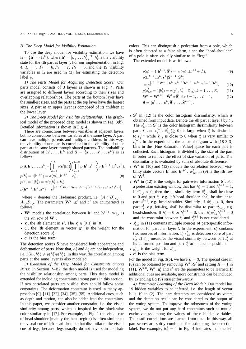
B. The Deep Model for Visibility Estimation

To use the deep model for visibility estimation, we haveh = {h1 · · ·hL}, where hl = [hl1 . . . h

lPl]T, hli is the visibility

state for the ith part at layer l. For our implementation in Fig.4, L = 3, P1 = 6, P2 = 7, P3 = 6, and the 19 visibilityvariables in h are used in (3) for estimating the detectionlabel y.

1) The Parts Model for Acquiring Detection Score: Ourparts model consists of 3 layers as shown in Fig. 4. Partsare assigned to different layers according to their sizes andoverlapping relationships. The parts at the bottom layer havethe smallest sizes, and the parts at the top layer have the largestsizes. A part at an upper layer is composed of its children atthe lower layer.

2) The Deep Model for Visibility Relationship: The graph-ical model of the proposed deep model is shown in Fig. 3(b).Detailed information is shown in Fig. 4.

There are connections between variables at adjacent layersbut no connections between variables at the same layer. A partcan have multiple parents and multiple children. In this way,the visibility of one part is correlated to the visibility of otherparts at the same layer through shared parents. The probabilitydistribution of h1, . . . ,hL and S = {s1, . . . sl, . . . sL} is asfollows:

p(S,h1, . . . ,hL)=

(L∏

l=1

p(sl|hl)

)(L−2∏l=1

p(hl|hl+1)

)p(hL−1,hL, sL),

p(hli = 1|hl+1) = σ(wl

i,∗hl+1 + cli), (8)

p(sli = 1|hli) = σ(glih

li + bli),

p(hL−1,hL, sL) = e

[hL−1T

WL−1hL+(cL−1)ThL−1+(cL+gL◦sL)

ThL

],

where ◦ denotes the Hadamard product, i.e. (A ◦ B) i,j =Ai,jBi,j . The parameters Wl, gl and cl are enumerated asfollows:

• Wl models the correlation between hl and hl+1, wli,∗ is

the ith row of Wl.• sli, the ith element in sl. The sli ∈ [0 1] in (8).• gli, the ith element in vector gl, is the weight for the

detection score sli.• cl is the bias term.

The detection scores S have considered both appearance anddeformation of parts. Note that, h l

i and hlj are not independent,i.e. p(hli, h

lj) �= p(hli)p(h

lj). In this way, the correlation among

parts at the same layer is also modeled.3) Extension of the Deep Model for Constraints among

Parts: In Section IV-B2, the deep model is used for modelingthe visibility relationship among parts. This deep model isextended for including constraints among parts in this section.If two correlated parts are visible, they should follow someconstraints. The deformation constraint is used in many ap-proaches [9], [11], [32], [34], [35], [55]. Additional cues, suchas depth and motion, can also be added into the constraints.In this paper, we consider another constraint, i.e. the visualsimilarity among parts, which is inspired by the block-wisecolor similarity in [17]. For example, in Fig. 1 the visual cueof head-shoulder (mainly the head region) is often similar tothe visual cue of left-head-shoulder but dissimilar to the visualcue of legs, because legs usually do not have skin and hair

colors. This can distinguish a pedestrian from a pole, whichis often detected as a false alarm, since the “head-shoulder”of a pole is often visually similar to its “legs”.

The extended model is as follows:

p(hli = 1|hl+1, Sl) = σ(wl

i,∗hl+1+ cli), (9)

p(hL−1,hL, sL|SL−1, SL)

= e

[hL−1T

WL−1hL+cL−1ThL−1+(cL+gL◦sL)

ThL

], (10)

p(sli,k = 1|hli) = σ(gli,kh

li + bli,k), k = 1, . . . ,K, (11)

Wl = Wl,0 + Wl ◦ Sl, for l = 1, . . . L− 1, (12)

S = {s1, . . . , sL, S1, . . . , SL−1}.

• Sl in (12) is the color histogram dissimilarity, which isobtained from input data. Denote the ith part at layer l by t li.The sli,j in Sl is the color histogram dissimilarity betweenparts tli and tl+1

j . sli,j(≥ 0) is large when tli is dissimilarto tl+1

j while sli,j is close to 0 when tli is very similar totl+1j . In the experiment, the color histogram with [18 3 3]

bins in the [Hue Saturation Value] space for each part iscollected. Each histogram is divided by the size of the partin order to remove the effect of size variation of parts. Thedissimilarity is evaluated by sum of absolute difference.

• Wl in (10) and (12) models the correlation between visi-bility state vectors hl and hl+1. wl

i,∗ in (9) is the ith rowof Wl.

• Wl in (12) is the weight for pair-wise information Sl. Fora pedestrian existing window that has hl

i = 1 and hl+1j = 1,

if wli,j < 0, then the dissimilarity term sli,j shall be close

to 0 and part tli, e.g. left-head-shoulder, shall be similar topart tl+1

j , e.g. head-shoulder. Similarly, if w li,j > 0, then

part tli, e.g. left-leg, shall be dissimilar to part tlj+1, e.g.head-shoulder. If hl

i = 0 or hl+1j = 0, then hliw

li,jh

l+1j = 0

and the constraint between tli and tl+1j is not considered.

• sli,k in (11) contains multiple sources of part-specific infor-mation for part i in layer l. In the experiment, s l

i containstwo sources of information: 1) sli,1 is detection score of parttli; 2) sli,2 measures the visual similarity between part tli atits deformed position and part tli at its anchor position.

• gli,k is the weight for sli,k.• cl is the bias term.For the model in Fig. 3(b), we have L = 3. The special case in(8) can be obtained by removing Wl◦Sl and setting K = 1 in(11). Wl,0, Wl, gl

i and cl are the parameters to be learned. Ifadditional cues are available, more constraints can be includedby extending Eq (9) straightforwardly.

4) Parameter Learning of the Deep Model: Our model has19 hidden variables to be inferred, i.e. the length of vectorh is 19 in (2). The part detectors are considered as votersand the detection result can be considered as the output ofthe voting system. To improve the robustness of the votingsystem, we do not put any hard constraints such as mutualexclusiveness among the values of these hidden variables.Their soft correlations are learned from data. In this way, allpart scores are softly combined for estimating the detectionlabel. For example, h3

2 = 1 in Fig. 4 indicates that the left

JOURNAL OF LATEX CLASS FILES, VOL. 11, NO. 4, DECEMBER 2012 6

side of a pedestrian is visible, but does not imply that the rightside is invisible. It does not imply that its sub-parts h2

2 andh25 must be visible either. If a pedestrian is fully visible, anyhli could be 1. Therefore, there are 219 possible combinationsof visibility variables of different parts to enumerate duringinference and the probability of each combination needs to beestimated.

Since the proposed model is a loopy graphical model, itis normally time consuming and hard to train. Hinton et al.[49], [52] proposed a fast learning algorithm for deep beliefnet (DBN) which has shown its success in many applications.In this work, we adopt a similar learning algorithm to trainour model. The difference between our model and DBN is asfollows:

1) Sl and sl for l = 1, . . . , L in our model are directlyestimated from input data by functions Sl = φ(x, l) andsl = ψ(x, l). In this model, we will not model p(x) andφ(x, l) is learned by supervised training.

2) With the term wli,∗ ◦ si,∗ added for hl

i and hidden nodessi,∗ connected with hl

i, each hidden unit hli now has

specific meaning related to the semantic meanings ofsli,∗ and si,∗ obtained from input data. Taking the termglis

li in (8) for pedestrian detection as an example, if

sli is the detection score of part i at layer l, then thehidden unit hl

i can be considered as the visibility of thatpart with hli = 1 meaning a visible part and hl

i = 0

meaning an occluded part. Without the terms g liTsli and

wli,∗ ◦ si,∗, which is the case in DBN, the meaning of

each hidden unit is not clear.3) In DBN, observed variables are arranged at the first layer

and connected to hidden variables at the second layer. Inour model, the observed variables S and s are connectedto hidden variables at many different layers.

Because of these differences, the learning algorithm of DBNcannot be directly applied to our model. We modified thetraining and inference algorithms in [49] when applying themto our model.

The training algorithm is to learn the parameters θ ={Wl,0,Wl,gl

i, cl} for l = 1, . . . , L and k = 1, . . . ,K in

(8), with two stages.

1) Stage 1: For l=1 to 2 { Train parameters for layer l andl + 1 using RBM. }

2) Stage 2: Fine-tune all the parameters by backpropagatingerror derivatives.

At Stage 1, the parameters are trained layer by layer andtwo adjacent layers are considered as an RBM that has thefollowing distributions:

p(hl,hl+1, sl+1|sl, Sl, Sl+1)

= e

[hlT

Wlhl+1+(cl+cl)Thl+(cl+1+cl+1)

Thl+1

],

p(hli = 1|hl+1, sl, Sl) = σ(wl

i,∗hl+1 + cli + gl

i

Tsli),

p(hl+1j = 1|hl, sl+1, Sl+1)=σ(hlTwl

∗,j+cl+1j +gl+1

j

Tsl+1j ),

p(sl+1i,k |hl+1) = σ(gl+1

i,k hl+1i + bl+1

i,k ),

p(h1, s1) = e∑

i,k g1i,kh1i+b1i,ks1i,k+c1ih

1i ,

Wl = Wl,0 + Wl ◦ Sl,

cl = [cl1 cl2 . . . cli . . .]

T , cli = gli

Tsli,

(13)

...

...

...

...

h1

h2

h3

W 1

W 2

yW 3S

Fig. 5. The BP network for fine tuning and estimating visibility.

where wli,∗ is the ith row of Wl and wl

∗,j is the jthcolumn of Wl, sli,k for k = 1, . . . ,K is the kth element invector sli, g

li,k is the kth element in vector gl

i of length K .K = 2 in our experiment. In the layer-wise pretraining, s 1 isconsidered as the observed variable and p(h1, s1) is consideredas the RBM for learning the g1i,k,and c1i in (13). Then h1

is fixed, h1 and s2 are considered as the visible vector fortraining p(h1,h2, s2|s1,x), similarly for p(h2,h3, s3|s2,x).The gradient of the log-likelihood for this RBM is computedas follows:

∂L(hl)

∂wl,0i,j

∝ (< hlih

l+1j >data − < hl

ihl+1j >model),

∂L(hl)

∂wli,j

∝ (< sli,jhlih

l+1j >data − < sli,jh

lih

l+1j >model),

∂L(hl)

∂cli∝ (< hl

i >data − < hli >model),

∂L(hl)

∂gli,k∝ (< hl

isli,k >data − < hl

isli,k >model), k = 1, 2,

(14)

where wl,0i,j and wl

i,j are the (i, j)th element in matricesWl,0 and Wl respectively. The contrastive divergence in [77]is used as the fast algorithm for learning the parameters in(13). In the appendix, we prove that this layer-wise trainingalgorithm is optimizing likelihood function p(h l) by a lowerbound

∑hl+1 Q(hl+1|hl) log p(hl+1,hl)

Q(hl+1|hl), where Q(hl+1|hl) is

the probability learned for layer l and l + 1 using RBM. AtStage 2, the variables are arranged as a backpropagation (BP)network as shown in Fig. 5 for fine tuning all parameters.

The inference stage is to infer the label y from detectionwindow features x. At the inference stage, we use the frame-work in (3) for obtaining p(y|x). And the 19 part visibilityvariables hl+1

j for (3) are obtained using the BP network inFig. 5, i.e.

hl+1j = p(hl+1

j = 1|h\hl+1j ,x) = p(hl+1

j = 1|hl,x)

= σ(hlTwl∗,j + cl+1

j + gl+1j

Tsl+1j ),

h1j = σ(c1j + g1

jTs1j ).

(15)

In order to reduce the bias of training data and regularizethe training process, we enforce the visibility correlationparameter Wl,0 in (9) to be non-negative. Therefore, ourtraining process has used the prior knowledge that negativecorrelation among the visibility of parts is unreasonable, e.g.the invisible left-leg shall not indicate the visible two-legs.Furthermore, the element w l

i,j of Wl in (8) is set to zeroif there is no connection between units h l

i and hl+1j in Fig.

4. Taking the parts in Fig. 1 as an example, the visibilityof the part left-leg is considered as not correlated with thevisibility of the part head-shoulder. For the extended modelin Section IV-B3, on the other hand, the visual dissimilarityamong different parts is considered as an important visual cue

JOURNAL OF LATEX CLASS FILES, VOL. 11, NO. 4, DECEMBER 2012 7

and there is not constraint for the elements in Wl in (9)(i.e.,we consider the visual dissimilarity between any two parts). Inthis way, we keep the most important correlation parametersbased on prior knowledge.

V. EXPERIMENTAL RESULTS

The proposed framework is evaluated on four datasets: Cal-tech [44], ETHZ [22] and Daimler [23] datasets are publiclyavailable; the CUHK occlusion dataset is constructed by us2.The INRIA training dataset in [6] is directly used to trainour approach if not specified. Occlusion information is notrequired during training. Once the model is learned fromthis training set, it is fixed and tested on the four datasetsmentioned above. Our deep model is to learn the visibilitycorrelations among different parts, which is feasible eventhough the INRIA training set does not have many occludedpedestrian samples. It shares similar spirit with some datareconstruction problems solved with deep models [80], [81].The data model is learned from positive samples withoutbeing corrupted. If any test sample is corrupted, its missingvalues can be reconstructed with the learned deep modelsin [80], [81]. In pedestrian detection, the performance mightget improved if the training set includes occluded positivesamples. However it will also take the risk of introducingbias, since the distribution of occlusion configurations in thetraining set could be different than the test set. Our currentexperimental results show that only using INRIA training setwithout many occlusions leads to good performance on varioustest datasets.

In the experiment, we use the modified HOG in [9] as thefeature for detection. HOG feature was proposed in [6] andmodified in [9]. The parts at the bottom layer and the head-shoulder part at the middle layer compute HOG features attwice the spatial resolution relative to the features computedby the other parts. In our implementation, the deformable part-based model in [9] is used for learning part detectors andmodeling the deformation among the 19 parts in Fig. 4. Theparts are arranged in the star model with the full body partbeing the root. Since the detection scores obtained from ourparts model are considered as the input of our deep model, thedeep model keeps unchanged if other deformable part-basedmodels and features are used.

The approaches HOG+SVM [6] and LatSVM-V2 [9] to becompared and our approach use the same features for part-based detection. They are also trained from the INRIA dataset.The evaluation criteria proposed in [44] is used. The labels andevaluation code provided by Dollar et al. online 3 is used forevaluating the Caltech dataset and the ETHZ dataset. As in[44], log-average miss rate is used to summarize the detectorperformance, computed by averaging miss rate at nine FPPIrates evenly spaced in log-space from 10−2 to 100.

A. Experimental Results on the CUHK Occlusion Dataset

Most existing pedestrian detection datasets are not specifi-cally designed for evaluating occlusion handling. For example,

2Available on www.ee.cuhk.edu.hk/∼xgwang/CUHK pedestrian.html3Available on www.vision.caltech.edu/ImageDatasets/CaltechPedestrians/

although the Caltech training dataset contains 192k pedestriansand 128k images, it is from 30 frames per second videosequences, where many frames are very similar to each other.In order to save computation and avoid evaluating nearly-the-same images, existing literatures [2], [17], [26], [44], [66],[66], [75], [82], [83] report the results on the Caltech datasetusing every 30th frame (starting with the 30th frame), i.e.4250 images in the Caltech training dataset are used forevaluation. In these 4250 images, only 105 images containoccluded pedestrians. If such datasets are used for evaluation,it is not clear how much improvement comes from occlusionhandling or other factors. In order to specifically comparepedestrian detection algorithms under occlusions, we constructthe CUHK occlusion dataset that mainly include images withoccluded pedestrians. All the 105 images containing occludedpedestrians in the 4250 Caltech training images and occludedimages from ETHZ, TUD-Brussels, INRA and Caviar datasetshave been included in the CUHK dataset. We also record 212images from surveillance cameras. The composition of thedataset is shown in Table I. The dataset contains 3476 non-occluded pedestrians and 2373 occluded pedestrians. Imagesare strictly selected according to the following criteria.

1. Each image contains at least one occluded pedestrian.2. Datasets Caviar and ETHZ are video sequences with high

frame rate, e.g. 25 frames per second for Caviar. In thesedatasets, the current frame may be very similar to the nextframe. In our dataset, the frame rate is reduced to ensurevariation among selected images.

3. The image shall not contain sitting humans, since it ispotentially controversial whether they should be detected aspedestrian or not.

Each pedestrian is labeled with a bounding box and a tagindicating whether the pedestrian is occluded or not. Since alot of occluded pedestrians in datasets like INRIA, ETHZ andTUD-Brussels are not considered as positive testing samples,the occluded pedestrians are relabeled in our dataset. Occludedpedestrians have been labeled in the Caltech dataset, theirlabels are unchanged in our dataset. Selected detection resultsof our approach on this dataset are shown in Fig. 7.

We evaluate the performance of our approach on occludedpedestrians and unoccluded pedestrians separately and com-pare with the two part-based models proposed by Zhu et al.[11] and LatSVM-V2 in [9] in Fig. 6. Our approach has similarperformance with [11] and [9] on unoccluded pedestrians andachieved 9% improvement on occluded pedestrians comparedwith [11] and [9] (the smaller the miss rate in the y-axisthe better). To investigate the effectiveness of using the deepmodel to estimate the visibility of parts, we also test our part-based model that directly sums up detection score using (4)and exclude the deep model. It has comparable performanceas [11] and [9] on occluded pedestrians. By including moreinformation of the pairwise visual dissimilarity among parts,the extended model introduced in Section IV-B3, i.e. Ours-D2,is better than the model in Section IV-B2, i.e. Ours-D1.

In order to investigate various schemes for integrating thepart detection scores, we conduct another set of experimentsin Fig. 6(c)-(f). They all use our parts model and thereforehave the same detection scores as input. Our-P in Fig. 6

JOURNAL OF LATEX CLASS FILES, VOL. 11, NO. 4, DECEMBER 2012 8

10−2

100

102

.10

.20

.30

.40

.50

.64

.801

false positives per image

mis

s ra

te

34% HOG+SVM

26% LatSvm−V2

26% Zhu

25% Ours−P

24% Ours−D1

24% Ours−D2

10−2

100

102

.10

.20

.30

.40

.50

.64

.801

false positives per image

mis

s ra

te

50% Rule

32% T(ε=0.5)

29% T(ε=0.4)

26% T(ε=0.2)

25% T(ε=0.05)

25% T(ε=0.1)

25% T(ε=0.01)

25% T(ε=0.001)

25% Ours−P

25% Ours−P

24% Ours−D1

24% Ours−D2

24% DBN

10−2

100

102

.10

.20

.30

.40

.50

.64

.801

false positives per image

mis

s ra

te

82% Max 1

78% Max 2

60% Max 4

39% Max 8

33% Max 10

27% Max 15

25% Max 18

25% Ours−P

24% Ours−D1

24% Ours−D2

(a) No occlusion (c) No occlusion (e) No occlusion

10−2

100

102

.40

.50

.64

.80

1

false positives per image

mis

s ra

te

73% HOG+SVM

65% LatSvm−V2

65% Zhu

64% Ours−P

59% Ours−D1

56% Ours−D2

10−2

100

102

.40

.50

.64

.80

1

false positives per image

mis

s ra

te

69% Rule

67% T(ε=0.5)

65% T(ε=0.4)

64% Ours−P

64% Ours−P

64% T(ε=0.2)

63% T(ε=0.001)

63% DBN

63% T(ε=0.01)

63% T(ε=0.05)

63% T(ε=0.1)

59% Ours−D1

56% Ours−D2

10−2

100

102

.40

.50

.64

.80

1

false positives per image

mis

s ra

te

96% Max 1

95% Max 2

86% Max 4

72% Max 8

68% Max 10

64% Ours−P

63% Max 15

63% Max 18

59% Ours−D1

56% Ours−D2

(b) With occlusion (d) With occlusion (f) With occlusion

Fig. 6. Experimental comparisons of different part-based models ((a)-(b)) and different schemes of integrating part detection scores ((c) - (f)) on the CUHKdataset for pedestrians without occlusions (upper row) and with occlusions (bottom row). Zhu denotes results of using the parts model proposed by Zhu etal. in [11]. Ours-P denotes results of using our parts model in Fig. 4 and directly summing up detection score however without the deep model. In thiscase, it is equivalent to computing the weighted mean of part scores. Ours-D1 and Ours-D2 denote the results of using our parts model and the deep modelintroduced in Section IV-B. Ours-D1 denotes the deep model in Section IV-B2 and Ours-D2 denotes the extended model in Section IV-B3. DBN denotes theresults of replacing our deep model by DBN. Rule denotes the results of using the rule in [67] for integrating our part scores. T(ε=ε0) denotes the results ofestimating visibility by hard-thresholding. Ti is learned from the training data such that ε0 percentage of parts in the positive training samples are consideredas occlusions. Max k denotes taking the k maximum part scores for computing the weighted mean.

Misseddetection

Falsepositive True positive

Caltech

INRIA

TUD-Brussels

Caviar

Our

ETHZ

Fig. 7. Selected detection results using our framework on the CUHK occlusion dataset. The sources of images are given. All results are obtained by usingthe same threshold. Blue rectangles in dashed lines are missed detections, green rectangles in solid lines are false positive windows, and red rectangles insolid lines are true positive detections.

TABLE ITHE COMPOSITION OF THE CUHK DATASET.Dataset Number of images selected

Caltech train [44] 105INRIA test [6] 70

TUD-Brussels [84] 110ETHZ [22] 211Caviar [85] 355

Our 212

is the weighted mean of part scores and the weights aretrained by linear SVM. Fig. 6(c) and (d) show the results ofestimating the visibility by thresholding the detection scores,

i.e. part score si is ignored if si < Ti. Using the same Ti

for all the parts is not optimal. Therefore, we assume thatdifferent parts have different threshold T i and obtain Ti fromtraining data. For each part, Ti is chosen such that certainpercentage ε(= 0.1%, 1%, 5%, 10%, 20%, 40%, 50%) of partson the positive training samples are considered as occlusions.The approach in [67] defines rule for estimating visibility ofparts and integrating detection scores. We use the same rulesproposed in [67] to integrate our part scores. As shown in Fig.6 (c) and (d), the rule based integration does not work well onour parts model although it has reported satisfactory results

JOURNAL OF LATEX CLASS FILES, VOL. 11, NO. 4, DECEMBER 2012 9

on the parts model in [67]. This may be due to the fact thatwe use different features and different parts model from [67].We cannot exactly obtain the results in [67] on our datasetbecause its implemenation is not available. The DBN in Fig.6 arranges all part detection scores as the bottom observedlayer and 3 layers of hidden units on top of the observed layeras shown in Fig. 3(c). The approach in [49] is then used fortraining parameters and classifying whether an input windowis a pedestrian or not. It is observed that directly applyingDBN to parts detection scores does not solve the occlusionproblem effectively. Fig. 6(e) and (f) show the results of takingk = 1, 2, 4, 8, 10, 15, 18 maximum part scores for computingthe weighted mean. The experimental results show that all theschemes discussed above perform worse than our deep model(represented by Ours −D2).

In another experiment, we investigate the robustness of themodel when the training dataset is under different levels ofdisturbances. The goal is systematically study if the occlusionstates in the training set has bias (e.g. left leg is morefrequently occluded than other parts), whether the performanceof the trained deep model will be deteriorated on test samplesoccluded in different ways. Results show that it is worsethan a properly trained deep model but still slightly betterthan directly summing up the part detection scores. Fig. 9shows the experimental results. In this experiment, we distortthe INRIA training dataset and obtain 3 distorted trainingdatasets Dstrt1 − Dstrt3. The distorted images are onlyused for training the parameters of the occlusion model butnot the part model. The negative training samples are keptunchanged. For a dataset, say Dstrt1, all positive trainingsamples have the same region replaced by randomly selectednegative patches. In this way, the detection scores s related tothis region are distorted for all positive samples. Fig. 8 showsthe examples of distorted positive examples. Dataset Dstrt1have the left leg and left torso replaced by negative patches,dataset Dstrt2 have the two legs replaced and dataset Dstrt3have the torso and legs replaced. All positive pedestrians inDstrt3 have about 3/4 region distorted. As shown by theexperimental results in Fig. 8, the distortion does influencethe detection performance of the deep model. All comparedapproaches have similar performance as that when pedestriansare not occluded. The performance on testing data degradesfor occluded pedestrians when distortion exists in the positivetraining samples, compared with Ours−D2, which is properlytrained. When the distortion is the largest, i.e. dataset Dstrt3,the detection performance is the worst. Even if about 3/4region of the pedestrian is distorted for all positive samplesin Dstrt3, the model still learns reasonable parameters andoutperforms the case when the part detection scores aredirectly summed up without the deep model, i.e. Ours-P. Thedeep model aims at learning the visibility relationship amongparts. The worst bias caused by the disturbed region, e.g. left-leg for the dataset Dstrt1, is to have negative relationshiplearned among parts, e.g. between left-leg and two-legs forthe dataset Dstrt1. With the non-negative enforcement onthe elements in Wl,0, negative relationship is impossible.Therefore, the relationship learned for the disturbed region iszero at the worst case, in which the deep model degenerates

Dstrt1 Dstrt3Dstrt2

Fig. 8. Selected original positive samples (1st column) and distorted positiveexamples with disturbance in dataset Dstrt1, Dstrt2 and Dstrt3 (2nd,3rd and 4th column). The same region is distorted in the same dataset. Thesame positive sample is distorted by the same negative sample. 2416 negativesamples are randomly selected for replacing the corresponding regions of the2416 positive samples.

into using no relationship and directly using part score fordetection. Since the relationship among undistorted parts, e.g.the relationship between left-head-shoulder and head-shoulder,is still effectively learned, the deep model outperforms the casewhere no relationship is used.

Fig. 10 shows the experimental results on different im-plementations of the deep model. Compared with the im-plementation that restricts the weights among hidden nodesto be non-negative (Ours-D2), the implementation withoutthis restriction increases the miss rate by 4% for pedestrianswithout occlusion and 3% for pedestrians with occlusion(Ours-D2-NW). Compared with the implementation (Ours-D2)that uses 19 hidden nodes for (3), the implementation that usesthe top 6 hidden nodes in Fig. 4 (Ours-D2-6h) for (3) increasesthe miss rate by 3% for pedestrians without occlusion and4% for pedestrians with occlusion. The implementation thatuses only BP for training (Ours-D2-BP) the model (withoutunsupervised RMB pre-training) increases the miss rate by 6%for pedestrians with occlusion. The number of rounds usedin Ours-D2-BP for BP is equal to the number of rounds forRBM used in Ours-D2 plus the number of rounds for BPused in Ours-D2. The implementation that uses only BP fortraining (Ours-D2-BP) the model increases the miss rate by6% for pedestrians with occlusion. The number of rounds usedin Ours-D2-BP for BP is equal to the number of rounds forRBM plus the number of rounds for BP used by Ours-D2. Theimplementation Ours-D2-NoOcc that only linearly combinesthe color histogram dissimilarity terms without the deep modelfor occlusion handling increases the miss rate by 6% forpedestrians with occlusion. Experimental results for Ours-D2-BP and Ours-D2-NoOcc on the Caltech Testing datasetare shown in Fig. 13. Theoretically, the issue of whetherunsupervised pre-training helps later supervised learning inthe same network is controversial and far from being decided.The empirical results on the two datasets show that indeed theunsupervised stage contributes to performance.

Although this paper focuses on using the deep modelfor pedestrian detection, the proposed deep model is alsoapplicable for estimating the visibility of parts. Fig. 11 showsthe visibility estimation results obtained from the deep model.

To investigate the execution time required by our model,we run the LatSVM-V2 and our parts model for 8 imageswith resolution 1280× 960. The experiment is run for 3 times

JOURNAL OF LATEX CLASS FILES, VOL. 11, NO. 4, DECEMBER 2012 10

10−2

100

.10

.20

.30

.40

.50

.64

.801

false positives per image

mis

s ra

te

25% Ours−P

24% Ours−D2

24% Ours−D−Dstrt3

24% Ours−D−Dstrt2

24% Ours−D−Dstrt1

10−2

100

.40

.50

.64

.80

1

false positives per imagem

iss

rate

64% Ours−P

63% Ours−D−Dstrt3

63% Ours−D−Dstrt2

62% Ours−D−Dstrt1

56% Ours−D2

(a) No occlusion (b) With occlusionFig. 9. Experimental results on the CUHK occlusion dataset for the deepmodel when the positive training data is distorted. Ours-D2 denotes the casewhen there is no distortion. Ours-D-Dstrt1 denotes results for the deep modeltrained on dataset Dstrt1. Similarly for Ours-D-Dstrt2 and Ours-D-Dstrt3.

10−2

100

.10

.20

.30

.40

.50

.64

.801

false positives per image

mis

s ra

te

28% Ours−D2−NW

27% Ours−D2−6h

26% Ours−D2−BP

24% Ours−D1

24% Ours−D2

24% Ours−D2−NoOcc

10−2

100

.40

.50

.64

.80

1

false positives per image

mis

s ra

te

62% Ours−D2−NoOcc

62% Ours−D2−BP

60% Ours−D2−6h

59% Ours−D1

59% Ours−D2−NW

56% Ours−D2

(a) No occlusion (b) With occlusionFig. 10. Experimental results on the CUHK occlusion dataset for differentimplementations of the deep model. Ours-D2 denotes the case when 19 hiddennodes are used for estimating detection label and the weights among hiddennodes to be non-negative. Ours-D2-6h denotes the case when 6 hidden nodesare used for estimating detection label. Ours-D2-NW denotes the case whenthe weights among hidden nodes are allowed to be negative.

and the difference in total execution time is less than 1%. Theaverage detection time required by our parts model is about 1.3times of that required by LatSVM-V2 on a 3.3GHz CPU withmulti-threading turned off. The most time consuming tasks,i.e. feature and SVM computation, for our parts model areimplemented by the same c code as the LatSVM-V2 providedby Felzenszwalb etc. online [86]. Our parts model contains25730 features and LatSVM-V2 contains 12741 features. Thenumber of features mainly influence the time required forcomputing SVM. According to our experiment, although ourparts model contains about 2 times the number of features ofLatSVM-V2, the execution time required by our parts modelfor computing SVM is less than 1.4 times the time requiredby LatSVM-V2. This might be caused by the fact that bothmodels compute SVM on the same feature window and takethe same execution time caused by cache miss, which is a mainfactor that influences the time required for computing SVMon sliding windows. The time required by our deep model forestimating visibility using the deep model is less than 10% ofthe time required by our part-based detector. Since our deepmodel has only 20 hidden variables in all for 3 layers, training

ImageImage Visibility

Occluded

Visible

Visibility Image Visibility Image Visibility

Fig. 11. Visibility estimated from the deep model. Black rectangle corre-sponds to invisible parts.

time for the deep model is also much less than that for theparts model.

B. Experimental Results on Caltech

The evaluated pedestrian detection approaches on the Cal-tech dataset are VJ [12], Shapelet [13], PoseInv [60], LatSVM-V1 [9], HikSVM [8], HOG+SVM [6], MultiFtr [43], HogLbp[21], Pls [20], FeatSynth [26], FtrMine [87], MultiFtr+CCS,MultiFtr+Motion [17] FPDW [66], ChnFtrs [2], CrossTalk[82], and MultiResC [83].

In the first experiment, the Caltech training dataset is usedas our testing set and the INRIA training dataset is used as ourtraining set to be consistent with most compared approaches,e.g. [17], [26], [87]. In Fig. 12, we compare with 16 ap-proaches under varying levels of occlusion. Compared withLatSVM-V2, our approach has 8%, 11% and 4% improvementon the log-average miss rate for pedestrians with no occlu-sions, partial occlusions and heavy occlusions respectively.Compared with the state-of-the-art approaches evaluated in[44] (excluding those using motions), our approach ranks asthe third, the second and the first for pedestrians with no oc-clusions, partial occlusions and heavy occlusions respectively.The two approaches MultiFtr+CCS [17] and ChnFtrs [2],which performed better than ours in the cases of no occlusionsand partial occlusions, both used a large number of extrafeatures such as color self-similarity, local sums, histograms,Haar features and their various generalizations beside HOG.Only HOG+SVM, LatSVM-V2 and our approach used theHOG features to compute the detection score. With morefeatures being included, the performance of our approach canbe further improved.

In the second experiment, the Caltech training dataset isused as our training set and the Caltech testing dataset, is usedas our testing set to be consistent with the approach MultiResC[83]. In this experiment, we evaluate the performance on thereasonable subset, which is the most popular portion of thedatasets. It consists of pedestrians with more than 49 pixelsin height, who are fully visible or partially occluded. Theapproach in [83] used the value [bbh − (a · bby + b)]2 as thegeometric constraint, where bbh is the bounding box height,bby is the y-location of the lower edge of the bounding box,a and b are linear regression parameters learned from theground truth bounding box of Caltech training dataset in [83].This geometric constraint is also used by our approach tomake a fair comparison with the approach in [83]. However,we obtain the linear regression parameters a and b fromdetection bounding boxes on the Caltech testing dataset in anunsupervised way, i.e. we need not the ground truth boundingbox for learning a and b. As shown by Fig. 13, our approachhas 4% average miss rate improvement compared with theMultiResC [83]. This geometric constraint is only used on theCaltech testing dataset but not used on other datasets, since[83] was not reported on other datasets.

Compared with the deformable model LatSVM-V2, ourdeep model reduces the miss rate from 63% to 44% on theCaltech testing dataset and from 51% to 46% on the ETHZdataset. By including more information of the pair-wise visual

JOURNAL OF LATEX CLASS FILES, VOL. 11, NO. 4, DECEMBER 2012 11

10−2

100

.20

.30

.40

.50

.64

.80

1

false positives per image

mis

s ra

te

96% VJ72% HOG+SVM69% LatSvm−V269% Pls62% FPDW62% CrossTalk61% Ours−D161% Ours−D258% MultiFtr+CSS

10−2

100

.50

.64

.80

1

false positives per image

mis

s ra

te

98% VJ92% HOG+SVM89% LatSvm−V287% Pls83% MultiFtr+CSS80% Ours−D180% CrossTalk80% FPDW78% Ours−D2

10−2

100

.64

.80

1

false positives per image

mis

s ra

te

99% VJ97% HOG+SVM96% Pls96% LatSvm−V296% CrossTalk95% FPDW94% MultiFtr+CSS93% Ours−D192% Ours−D2

Fig. 12. Experimental results on the Caltech training dataset for pedestrians under no occlusions (left), partial occlusions (center) and heavy occlusions(right). The ratio of visible area is larger than 0.65 for partial occlusions and [0.2 0.65] for heavy occlusions. The log-average miss rate of our model is 60%for no occlusions, 79% for partial occlusions and 92% for heavy occlusions.

dissimilarity among parts, the extended model introduced inSection IV-B3, i.e. Ours-D2, performs better than the modelin Section refSubSec:DBNOur, i.e. Ours-D1.

C. Experimental Results on ETHZ

The experimental results on the ETHZ testing sequencesare shown in Fig. 13. It is reported in [44] that LatSvm-V2 has the best performance among the 14 state-of-the-artapproaches evaluated on the ETHZ dataset. It can be seenthat our approach has 5% improvement over LatSVM-V2. TheETHZ dataset consists of 3 testing video sequences. Table IIshows the miss rates at 1 FPPI for the 3 sequences. The resultsof ISF are obtained from [67]. The results of HOG+SVMand LatSvm-V2 are obtained from [44] using the results andevaluation code provided online. Our model performs betterthan the traditional deep learning approach [75] on both ETHZand Caltech testing dataset.

D. Experimental Results on Daimler

The experimental results on the Daimler benchmark testingdata in [23] are shown in Fig. 14. Since the dataset is usedfor occluded pedestrian classification instead of detection,false positive versus detection rate is used for evaluation(the larger the detection rate in the y-axis the better). Sinceour focus is on detection for single images, we only usethe image intensity for all evaluated algorithms. Comparedwith LatSVM-V2, our approach has similar performance onunoccluded pedestrian, and our approach achieves about 20%detection rate improvement for occluded pedestrian. LatSVM-V2, HOG+SVM and our approach in Fig. 14 are trained onINRIA for consistency with previous experimental results.Since all the results in [23] are trained on the Daimler trainingdata and have different implementation of HOG feature fromours, we did not show the results in [23]. For example, theHOG+SVM trained on INRIA using the code in [9] havequite different result from the HOG+SVM trained on Daimlertraining data reported in [23].

VI. DISCUSSION

In this paper, the star model is used to model the deforma-tion correlation among parts, because the star model is widelyused in pedestrian detection and many recent papers [9], [83]based on the star model achieved the state-of-the-art resultson both the ETH and the Caltech dataset. If it is replacedwith other part models like the tree model [11], [32], [38],

10−3

10−2

10−1

100

101

102

103

.20

.30

.40

.50

.64

.80

1

false positives per image

mis

s ra

te

95% VJ

91% Shapelet

86% PoseInv

80% LatSvm−V1

77% ConvNet

74% FtrMine

73% HikSvm

68% HOG+SVM

68% MultiFtr

68% HogLbp

63% LatSvm−V2

62% Pls

61% MultiFtr+CSS

60% FeatSynth

57% FPDW

56% ChnFtrs

54% CrossTalk

50% Ours−D2−NoOcc

48% MultiResC

48% Ours−D2−BP

46% Ours−D1

44% Ours−D2

10−3

10−2

10−1

100

101

.20

.30

.40

.50

.64

.80

1

false positives per image

mis

s ra

te

90% VJ64% HOG+SVM61% MultiFtr+CSS60% FPDW55% Pls52% CrossTalk51% LatSvm−V250% ConvNet47% Ours−D146% Ours−D2

Fig. 13. Experimental results on Caltech Test dataset (top) and ETHZ dataset(bottom).

TABLE IIMISS RATE AT 1 FPPI FOR DIFFERENT APPROACHES. SEQ 1 (BAHNHOF)

HAS 999 FRAMES, SEQ 2 (JELMOLI) HAS 450 FRAMES AND SEQ 3(SUNNY DAY) HAS 354 FRAMES.

Seq 1 Seq 2 Seq 3ISF [67] 47% 38% 52%

HOG+SVM [6] 34% 44% 44%LatSvm-V2 [9] 30% 34% 32%

Ours 23% 33% 26%

loopy graph models [36] and complete graph models [63],our approach cannot be directly used in a straightforward way.However, it is still feasible after certain modification. Take thetree model as an example. The appearance score s li and thedeformation score dli need to be treated separately in (9)-(12).

0.05 0.1 0.15 0.2 0.250.7

0.8

0.9

1

False positives rate(Non−occluded)

Det

ectio

n ra

te

Ours−D2LatSVM−V2HOG+SVM

0.05 0.1 0.15 0.2 0.250.2

0.4

0.6

0.8

1

False positives rate(Occluded)

Fig. 14. Experimental results on Daimler occlusion dataset.

JOURNAL OF LATEX CLASS FILES, VOL. 11, NO. 4, DECEMBER 2012 12

The terms alidlih

l+1i +bli(1−hl+1

i ) related to dli depend on thevisibility hl+1

i of the parent part. If the parent part is visible,i.e. hl+1

i = 1, the penalty term is alidli, which depends on

the deformation score; otherwise, it is a constant b li as thedeformation score has become meaningless. Both a l

i and bliare parameters to be learned. This still leads to RBM, W l in(12) becomes Wl = Wl,0 + Wl,1 ◦ Sl + Wl,2 ◦ Dl. Thisis a future work. Our design of parts model is based on theknowledge about the constituents of human beings. Designand learning of new parts models that is optimized for humandetection is a possible way of improving the detection result.Since our deep model takes the detection scores of parts asinput, it is very flexible to incorporate with new features [27],[75] and new deformable part-based models.

The detection score is assumed to be provided in order tobe independent of detectors and features. However, interactionbetween the deep model and specific detector is a futurework for improvement. For example, since features can belearned by a deep model, e.g. the one in [27], it is possibleto incorporate the DBN into the learning of the part-baseddetector and estimating the visibility. It is also an interestingand open question of how to integrate the estimation of partlocations into the deep model.

Although we only use single image pixel values for detec-tion. The extended deep model in (9) has considered multiplesources of information and is naturally applicable for multiplecues like depth, motion and segmentation.

This paper estimates the detection label using the meanfield approximation in (3) for faster speed. Investigation onthe use of other methods for obtaining detection label fromthe visibility states of parts is a potential way of improvingdetection accuracy.

This paper aims at modeling occlusion at part level. How-ever, modeling occlusion at pixel level is a promising directionfor handling occlusion. For example, the masked RBM in [88]can be used for explicitly modeling occlusion boundaries inimage patches by factoring the appearance of a patch regionfrom its shape.

The main contribution of this paper is to learn the visibilityrelationship among parts using a hierarchical probabilisticmodel. Both directed model and undirected models can beused for learning this relationship. DBN is a combinationof undirected graphical model at the top layer and directedgraphical model at the other layers. Directed graphical modelsoften lead to the explaining away problem, in which recoveringthe posterior p(h|x) is often computationally challenging andeven intractable, especially when h is discrete [89]. The DBNstyle model is chosen because it is easy for inference and hasfast training algorithm [49] that can find a fairly good set ofparameters quickly.

VII. CONCLUSION

This paper describes a probabilistic framework forpedestrian detection with occlusion handling. It effectivelyestimates the visibility of parts at multiple layers and learnstheir relationship with the proposed deep model. Since ittakes the detection scores of parts as input, it is very flexible

to incorporate with new features and other deformable part-based models. Through extensive experimental comparisonon multiple datasets, various schemes of integrating partdetectors are investigated. Our approach outperforms thestate-of-the-arts especially on pedestrian data with occlusions.

Acknowledgment: This work is supported by the GeneralResearch Fund sponsored by the Research Grants Council ofHong Kong (project No. CUHK417110 and CUHK417011)and National Natural Science Foundation of China (projectno. 61005057).

REFERENCES

[1] P. Viola and M. Jones, “Robust real-time face detection,” IJCV, vol. 57,no. 2, pp. 137–154, 2004.

[2] P. Dollar, Z. Tu, P. Perona, and S. Belongie, “Integral channel features,”in BMVC, 2009.

[3] B. Wu and R. Nevatia, “Detection of multiple, partially occluded humansin a single image by bayesian combination of edgelet part detectors,” inICCV, 2005.

[4] O. Barinova, V. Lempitsky, and P. Kohli, “On detection of multipleobject instances using hough transforms,” in CVPR, 2010.

[5] K. Mikolajczyk, B. Leibe, and B. Schiele, “Multiple object classdetection with a generative model,” in CVPR, 2006.

[6] N. Dalal and B. Triggs, “Histograms of oriented gradients for humandetection,” in CVPR, 2005.

[7] M. Enzweiler and D. Gavrila, “Integrated pedestrian classification andorientation estimation,” in CVPR, 2010.

[8] S. Maji, A. C. Berg, and J. Malik, “Classification using intersectionkernel support vector machines is efficient,” in CVPR, 2008.

[9] P. Felzenszwalb, R. B. Grishick, D.McAllister, and D. Ramanan.,“Object detection with discriminatively trained part based models,” IEEETrans. PAMI, vol. 32, pp. 1627–1645, 2010.

[10] A. Vedaldi, V. Gulshan, M. Varma, and A. Zisserman, “Multiple kernelsfor object detection,” in ICCV, 2009.

[11] L. Zhu, Y. Chen, A. Yuille, and W. Freeman, “Latent hierarchicalstructural learning for object detection,” in CVPR, 2010.

[12] P. Viola, M. J. Jones, and D. Snow, “Detecting pedestrians using patternsof motion and appearance,” IJCV, vol. 63, no. 2, pp. 153–161, 2005.

[13] P. Sabzmeydani and G. Mori, “Detecting pedestrians by learning shapeletfeatures,” in CVPR, 2007.

[14] B. Leibe, E. Seemann, and B. Schiele, “Pedestrian detection in crowdedscenes,” in CVPR, 2005.

[15] C. Lampert, M. Blaschko, and T. Hofmann, “Beyond sliding windows:object localization by efficient subwindow search,” in CVPR, 2008.

[16] F. Porikli, “Integral histogram: a fast way to extract histograms incartesian spaces,” in CVPR, 2005.

[17] S. Walk, N. Majer, K. Schindler, and B. Schiele, “New features andinsights for pedestrian detection,” in CVPR, 2010.

[18] Q. Zhu, M.-C. Yeh, K.-T. Cheng, and S. Avidan, “Fast human detectionusing a cascade of histograms of oriented gradients,” in CVPR, 2006.

[19] O. Tuzel, F. Porikli, and P. Meer, “Pedestrian detection via classificationon riemannian manifolds,” IEEE Trans. PAMI, vol. 30, no. 10, pp. 1713–1727, Oct. 2008.

[20] W. Schwartz, A. Kembhavi, D. Harwood, and L. Davis, “Humandetection using partial least squares analysis,” in ICCV, 2009.

[21] X. Wang, X. Han, and S. Yan, “An hog-lbp human detector with partialocclusion handling,” in CVPR, 2009.

[22] A. Ess, B. Leibe, and L. V. Gool, “Depth and appearance for mobilescene analysis,” in ICCV, 2007.

[23] M. Enzweiler, A. Eigenstetter, B. Schiele, and D. M. Gavrila, “Multi-cue pedestrian classification with partial occlusion handling,” in CVPR,2010.

[24] M. Enzweiler and D. M. Gavrila, “A multilevel mixture-of-expertsframework for pedestrian classification,” IEEE Trans. Image Process.,vol. 20, no. 10, pp. 2967–2979, 2011.

[25] N. Dalal, B. Triggs, and C. Schmid, “Human detection using orientedhistograms of flow and appearance,” in ECCV, 2006.

[26] A. Bar-Hillel, D. Levi, E. Krupka, and C. Goldberg, “Part-based featuresynthesis for human detection,” in ECCV, 2010.

[27] M. Norouzi, M. Ranjbar, and G. Mori, “Stacks of convolutional restrictedboltzmann machines for shift-invariant feature learning,” in CVPR, 2009.

JOURNAL OF LATEX CLASS FILES, VOL. 11, NO. 4, DECEMBER 2012 13

[28] A. Smeulders, T. Gevers, N. Sebe, and C. Snoek, “Segmentation asselective search for object recognition,” in ICCV, 2011.

[29] M. Enzweiler and D. Gavrila, “A mixed generative-discriminative frame-work for pedestrian classification,” in CVPR, 2008.

[30] C. Mikolajczyk, C. Schmid, and A. Zisserman, “Human detection basedon a probabilistic assembly of robust part detectors,” in ECCV, 2004.

[31] H. Azizpour and I. Laptev, “Object detection using strongly-superviseddeformable part models,” in ECCV, 2012.

[32] P. F. Felzenszwalb and D. P. Huttenlocher, “Pictorial structures for objectrecognition,” IJCV, vol. 61, pp. 55–79, 2005.

[33] M. Andriluka, S. Roth, and B. Schiele, “Pictorial structures revisited:people detection and articulated pose estimation,” in CVPR, 2009.

[34] L. Bourdev, S. Maji, T. Brox, and J. Malik, “Detecting people usingmutually consistent poselet activations,” in ECCV, 2010.

[35] L. Bourdev and J. Malik, “Poselets: body part detectors trained using3D human pose annotations,” in ICCV, 2009.

[36] Y. Wang, D. Tran, and Z. Liao, “Learning hierarchical poselets forhuman parsing,” in CVPR, 2011.

[37] Y. Yang and D. Ramanan, “Articulated pose estimation with flexiblemixtures-of-parts,” in CVPR, 2011.

[38] M. Sun and S. Savarese, “Articulated part-based model for joint objectdetection and pose estimation,” in ICCV, 2011.

[39] C. Desai and D. Ramanan, “Detecting actions, poses, and objects withrelational phraselets,” in ECCV, 2012.

[40] M. Everingham, L. V. Gool, C. K. I.Williams, J.Winn, and A. Zisserman,“The pascal visual object classes (voc) challenge,” IJCV, vol. 88, no. 2,pp. 303–338, 2010.

[41] S. V. Lab, “http://www.image-net.org/challenges/lsvrc/2011/,” accessedin 2012.

[42] J. Deng, W. Dong, R. Socher, L.-J. Li, K. Li, and L. Fei-Fei, “Imagenet:a large-scale hierarchical image database,” in CVPR, 2009.

[43] C. Wojek and B. Schiele, “A performance evaluation of single and multi-feature people detection,” in DAGM, 2008.

[44] P. Dollar, C. Wojek, B. Schiele, and P. Perona, “Pedestrian detection:an evaluation of the state of the art,” IEEE Trans. PAMI, vol. 34, no. 4,pp. 743 – 761, 2012.

[45] D. Geronimo, A. M. Lopez, A. D. Sappa, and T. Graf, “Survey onpedestrian detection for advanced driver assistance systems,” IEEETrans. PAMI, vol. 32, no. 7, pp. 1239–1258, 2010.

[46] M. Enzweiler and D. M. Gavrila, “Monocular pedestrian detection:survey and experiments,” IEEE Trans. PAMI, vol. 31, no. 12, pp. 2179–2195, 2009.

[47] S. Munder and D. M. Gavrila, “An experimental study on pedestrianclassification,” IEEE Trans. PAMI, vol. 28, no. 11, pp. 1863–1868, 2006.

[48] S. Dai, M. Yang, Y. Wu, and A. Katsaggelos, “Detector ensemble,” inCVPR, 2007.

[49] G. E. Hinton, S. Osindero, and Y. Teh, “A fast learning algorithm fordeep belief nets,” Neural Computation, vol. 18, pp. 1527–1554, 2006.

[50] H. Lee, R. Grosse, R. Ranganath, and A. Y. Ng, “Convolutionaldeep belief networks for scalable unsupervised learning of hierarchicalrepresentations,” in ICML, 2009.

[51] Y. Bengio, “Learning deep architectures for AI,” Foundations and Trendsin Machine Learning, vol. 2, no. 1, pp. 1–127, 2009.

[52] G. E. Hinton and R. R. Salakhutdinov, “Reducing the dimensionality ofdata with neural networks,” Science, vol. 313, no. 5786, pp. 504 – 507,July 2006.

[53] M. Ranzato, J. Susskind, V. Mnih, and G. Hinton, “On deep generativemodels with applications to recognition,” in CVPR, 2011.

[54] K. Jarrett, K. Kavukcuoglu, M. Ranzato, and Y. LeCun, “What is thebest multi-stage architecture for object recognition?” in CVPR, 2009.

[55] M. Pedersoli, J. Gonzalez, A. D. Bagdanov, and J. J. Villanueva, “Re-cursive coarse-to-fine localization for fast object detection,” in ECCV,2010.

[56] R. Girshick, P. Felzenszwalb, and D. McAllester, “Object detection withgrammar models,” in NIPS, 2011.

[57] A. Mohan, C. Papageorgiou, and T. Poggio, “Example-based objectdetection in images by components,” IEEE Trans. PAMI, vol. 23, no. 4,pp. 349–361, 2001.

[58] B. Wu and R. Nevatia, “Detection and tracking of multiple, partiallyoccluded humans by bayesian combination of edgelet based part detec-tors,” IJCV, vol. 75, no. 2, pp. 247–266, 2007.

[59] ——, “Cluster boosted tree classifier for multiview, multi-pose objectdetection,” in ICCV, 2007.

[60] Z. Lin and L. Davis, “A pose-invariant descriptor for human detectionand segmentation,” in ECCV, 2008.

[61] J. Gall and V. Lempitsky, “Class-specific hough forests for objectdetection,” in CVPR, 2009.

[62] M. Pedersoli, A. Vedaldi, and J. Gonzalez, “A coarse-to-fine approachfor fast deformable object detection,” in CVPR, 2011.

[63] M. Bergtholdt, J. H. Kappes, S. Schmidt, and C. Schnorr, “A study ofparts-based object class detection using complete graphs,” IJCV, vol. 87,no. 1-2, pp. 93–117, 2010.

[64] B. Leibe, A. Leonardis, and B. Schiele, “Combined object categorizationand segmentation with an implicit shape model,” in In ECCV Workshopon Stat. Learn. in Comp. Vis, 2004.

[65] ——, “Robust object detection with interleaved categorization andsegmentation,” IJCV, vol. 77, no. 1-3, pp. 259–289, 2008.

[66] P. Dollar, S. Belongie, and P. Perona, “The fastest pedestrian detectorin the west,” in BMVC, 2010.

[67] G. Duan, H. Ai, and S. Lao, “A structural filter approach to humandetection,” in ECCV, 2010.

[68] T. Wu and S. Zhu, “A numeric study of the bottom-up and top-downinference processes in and-or graphs,” IJCV, vol. 93, no. 2, pp. 226–252,Jun. 2011.

[69] B. Wu and R. Nevatia, “Detection and segmentation of multiple,partially occluded objects by grouping, merging, assigning part detectionresponses,” IJCV, vol. 82, no. 2, pp. 185–204, 2009.

[70] Y. Lin, T. Liu, and C. Fuh, “Fast object detection with occlusion,” inECCV, 2004.

[71] T. Gao, B. Packer, and D. Koller, “A segmentation-aware object detectionmodel with occlusion handling,” in CVPR, 2011.

[72] V. D. Shet, J. Neumann, V. Ramesh, and L. S. Davis, “Bilattice-basedlogical reasoning for human detection,” in CVPR, 2007.

[73] Z. Lin, L. S. Davis, D. Doermann, and D. DeMenthon, “Hierarchicalpart-template matching for human detection and segmentation,” in ICCV,2007.

[74] P. Luo, X. Wang, and X. Tang, “Hierarchical face parsing via deeplearning,” in CVPR, 2012.

[75] P. Sermanet, K. Kavukcuoglu, S. Chintala, and Y. Lecun, “Pedestriandetection with unsupervised and multi-stage feature learning,” in CVPR,2013.

[76] P. Smolensky, Information processing in dynamical systems: foundationsof harmony theory. Cambridge, MA, USA: MIT Press, 1986. [Online].Available: http://dl.acm.org/citation.cfm?id=104279.104290

[77] G. E. Hinton, “Training products of experts by minimizing contrastivedivergence,” Neural Computation, vol. 14, pp. 1771–1800, 2002.

[78] A. Hyvarinen, “Estimation of non-normalized statistical models usingscore matching,” J. of Machine Learning Research, vol. 6, pp. 695–709,2005.

[79] J. Sohl-Dickstein, P. Battaglino, and M. R. DeWeese, “Minimum prob-ability flow learning,” in ICML, 2011.

[80] H. Poon and P. Domingos, “Sum-product networks: A new deep archi-tecture,” in UAI, 2011.

[81] Y. Tang, R. Salakhutdinov, and G. Hinton, “Robust boltzmann machinesfor recognition and denoising,” in CVPR, 2012.

[82] P. Dollar, R. Appel, and W. Kienzle, “Crosstalk cascades for frame-ratepedestrian detection,” in ECCV, 2012.

[83] D. Park, D. Ramanan, and C. Fowlkes, “Multiresolution models forobject detection,” in ECCV, 2010.

[84] C. Wojek, S. Walk, and B. Schiele, “Multi-cue onboard pedestriandetection,” in CVPR, 2009.

[85] R. Fisher, “homepages.inf.ed.ac.uk/rbf/caviar/,” accessed in 2012.[Online]. Available: homepages.inf.ed.ac.uk/rbf/CAVIAR/

[86] P. F. Felzenszwalb, R. B. Girshick, and D. McAllester, “www.cs.brown.edu/∼pff/latent/,” accessed in 2012.

[87] P. Dollar, Z. Tu, H. Tao, and S. Belongie, “Feature mining for imageclassification,” in CVPR, 2007.

[88] N. Le Roux, N. Heess, J. Shotton, and J. Winn, “Learning a generativemodel of images by factoring appearance and shape,” Neural Computa-tion, vol. 23, no. 3, pp. 593–650, 2011.

[89] Y. Bengio, A. Courville, and P. Vincent, “Representation learning: Areview and new perspectives,” IEEE Trans. PAMI, vol. 35, no. 8, pp.1798–1828, 2013.

View publication statsView publication stats