JOURNAL OF LA On Compressive Orthonormal Sensing - Yingbin Liang's...

JOURNAL OF LATEX CLASS FILES, VOL. 14, NO. 8, AUGUST 2015 1

On Compressive Orthonormal SensingYi Zhou, Huishuai Zhang, and Yingbin Liang,

Abstract—The Compressive Sensing (CS) approach for recov-ering sparse signal with orthonormal measurements has beenstudied under various notions of coherence. However, existingnotions of coherence either do not exploit the structure of theunderlying signal, or are too complicated to provide an explicitsampling scheme for all orthonormal basis sets. Consequently,there is lack of understanding of key factors that guide the sam-pling of CS with orthonormal measurements and achieve as lowsample complexity as possible. In this paper, we introduce anewnotion of π-coherence that exploits both the sparsity structureof the signal and the local coherence. Based onπ-coherence, wepropose a sampling scheme that is adapted to the underlyingtrue signal and is applicable for CS under all orthonormalbasis. Our scheme outperforms (within a constant factor) existingsampling schemes for orthonormal measurements, and achieves anear-optimal sample complexity (within some logarithm factors)for several popular choices of orthonormal basis. Furthermore,we characterize the necessary sampling scheme for CS withorthonormal measurements. We then propose a practical multi-phase implementation of our sampling scheme, and verify itsadvantage over existing sampling schemes via application toMagnetic Resonance Imaging (MRI) in Medical Science.

Index Terms—Compressive Sensing, Orthonormal, Coherence.

I. I NTRODUCTION

With ever growing data size in signal processing appli-cations, taking full number of linear measurements of thesignal suffers from both high cost and low efficiency. In thepast decade, numerous work focus on recovering signals withreduced number of linear measurements by exploiting specialstructures of the signals. Among them, the sparsity of thesignal is found to be the key factor to reduce the samplecomplexity [1], [2], [3], [8]. This leads to the developmentof the so called Compressive Sensing (CS) technique, whichhas been successfully applied to various applications suchassparse MRI [4], face recognition [5], background subtraction[6] and photo-acoustic tomography [7], just to name a few.

We consider an orthonormal setting of CS, which consistsof a pair of orthonormal basisΨ,Φ ∈ Cn×n with basisvectors Ψ := [ψT

1 ; ...;ψTn ], Φ := [φT

1 ; ...;φTn ], and an

underlying true signalx0 ∈ Cn. The basisΨ provides a sparse

representation of the true signal, i.e.,θ0 = Ψx0 is assumedto be s-sparse. The basisΦ corresponds to the space overwhich the orthonormal measurements〈φj ,x0〉nj=1 are taken.Compressive sensing aims to recover the true signalx0 bytaking a few number of measurements. To be specific, denoteΩ ⊂ 1, . . . , n as the index set of the sampled orthonormal

Yi Zhou, Huishuai Zhang and Yingbin Liang are with the Department ofElectrical Engineering and Computer Science, Syracuse University, Syracuse,NY, e-mail: [email protected].

Manuscript received April 19, 2015; revised August 26, 2015.

measurements, and denoteΦΩ as Φ restricted on the rowswith index inΩ. Then CS aims to recoverx0 via

(P) minx∈Cn

‖Ψx‖1 s.t. ΦΩx = ΦΩx0.

A fundamental problem is to characterize the number ofsamples that guarantees problem(P) uniquely recover theunderlying signal. It has been well understood that samplecomplexity is highly related to sampling schemes, and threetypes of sampling schemes have been considered so far.

(a) Uniform sampling is considered in [9], in which eachorthonormal measurementφj , j = 1, · · · , n is equally likelyto be taken. It has been shown via a RIPless theory thatthe sample complexity depends on the following notion ofcoherence

(Mutual Coherence) µ(Ψ,Φ) := max1≤i,j≤n

|〈ψi,φj〉|2,

and is of the orderO(µ(Ψ,Φ)sn log n). In the low mutualcoherence regime (i.e.µ(Ψ,Φ) = O(1/n)) this samplecomplexity is order-wise optimal up to a logarithm factor.However, the sample complexity scales as large as the trivialorderO(n logn) if any pair of the basis vectors are exactlyaligned (i.e. maximally coherent) with each other.

(b) Measurement-adaptive sampling scheme was studiedin [10], [11], in which each orthonormal measurementφj issampled with probability being proportional to the so-calledlocal coherence, i.e.,

(Local Coherence) µ(Ψ,φj) := max1≤i≤n

|〈ψi,φj〉|2. (1)

The local coherence is determined by the basis pair and can beviewed as mutual coherence localized at thej-th measurement.It was shown in [10] that the sample complexity is of theorderO(∑j µ(Ψ,φj)s log

3 s logn)) via a RIP argument, andwas further improved toO(∑j µ(Ψ,φj)s log s logn)) via aRIPless argument in [11].

(c) Measurement-and-signal adaptive sampling schemewas proposed in [11]. There, the sampling of the orthonor-mal measurements is based on some complicated notions ofcoherence1, which are related to both the support informationof the underlying true signal and the basis pair. Only underΨ being the bivariate Haar wavelet basis andΦ being thediscrete Fourier basis, the sampling scheme is given in explicitform, and sample complexity is shown to be on the orderO(s log s logn).

The focus of this paper is to resolve remaining issues forthe third type of sampling scheme. The notion of coherenceintroduced in [11] does not yield a universal sampling schemefor recovering the true signal in all orthonormal basis pairs,and may not be the real underlying quantity that governs

1For simplicity we do not present them here.


the sample complexity. Hence, our goal is to find out thefundamental notion of coherence to guide the design of thesampling scheme, which 1) is adapted to the underlying truesignal; 2) is generally applicable to all basis pairs; and 3)yields better sample complexity.

A. Main Contributions

We propose the new notion ofπ-coherence (see Defini-tion 1) to capture how an orthonormal measurementφj iscoherent with the subspace where the true signal lies. Basedon the notion ofπ-coherence, we propose a Bernoulli samplingscheme that is generally applicable for all pairs of orthonormalbasis.

Our sampling scheme reveals the relationship among samplecomplexity, sparsity structure of the true signal and coherencepattern of the basis pair. We further show that our schemeachieves lower sample complexity (within a constant factor)than uniform sampling [8], measurement-adaptive sampling[10] and measurement-and-signal adaptive sampling [11]. Forseveral popular choices of orthonormal basis pairs, we showthat our sampling scheme achieves a near-optimal samplecomplexity (within some logarithm factors). Furthermore,wecharacterize the fundamental necessary sampling scheme forCS with orthonormal measurements.

Our technical proof introduces a weighted infinity normto control the concentration bounds in a tighter way. Con-sequently, these new concentration bounds avoid involvingcomplicated notions of coherence as those in [11], and lead toour notion of coherence that has an intuitive physical meaningon the sparsity structure of the signal and the coherence patternof the orthonormal basis pair.

For practical applications, we propose a multi-phase versionof our sampling scheme, which iteratively learns the subspaceinformation of the true signal and and updates the samplingscheme in the next phase.

B. Related Work

Various kinds of sampling schemes have been proposed forCS with orthonormal measurements. Some schemes are empir-ically oriented [12], [13], [14], [15], where the schemes weredemonstrated to be useful in specific applications. Closelytoour work are schemes theoretically oriented such as uniformsampling [8], [9], mixture of full sampling in finite regime anduniform sampling in asymptotic regime [16], measurement-adaptive sampling [10], [11], and measurement-and-signaladaptive sampling [11]. Our work falls into the last type ofsampling scheme that is adapted to both the underlying truesignal and the basis pair. Differently from [11] which explicitlyderives sampling scheme only for a specific basis pair, ourscheme is generally applicable to all orthonormal basis pairsand yields a better sample complexity.

There is another series of work on adaptive compressivesensing [17], [18], [19]. There, the focus was on recoveringthe support of the signal via adapting the distribution fromwhich the random measurements are generated, and do notinvolve any notion of coherence. In contrast, we are interested

in recovering the signal by sampling deterministic orthonormalmeasurements based on our notion of coherence.

Adaptive sampling has also been considered in matrix-related problems by exploiting the leverage score [20], [21],[22], which is related to the projections of canonical unitvectors onto row/column spaces of the matrix. In particular,[22] proposed a sampling scheme that is adapted to the lever-age scores of each entry of the matrix for matrix completionproblems.

C. Organization and Notations

This paper proceeds as follows. Section II introduces thesignal model and our notion of coherence; In Section III wepresent our sampling scheme and analyze the performanceguarantee of the sampling scheme; In Section IV we proposea multi-phase algorithm to illustrate how to implement oursampling scheme in practice; In Section V we present variousnumerical experiments to demonstrate our theoretical charac-terization, and finally we conclude the paper in Section VI.

We adopt the following notations in the paperx0: the underlying signal to recover;Ψ,Φ: the representation basis and measurement basis;Ω: the index set of sampled measurements;θ0: the representation ofx0 in basisΨ;S: support set ofθ0;Π: the subspace ofΨ wherex0 lies in.‖ · ‖p: Euclideanlp norm;‖ · ‖: spectral norm of an operator;I,H,F : the canonical basis, bivariate Haar wavelet basisand discrete Fourier basis, respectively.

II. SIGNAL MODEL AND π-COHERENCE

Suppose that the representation of signalx0 in basisΨ, i.e.θ0 = Ψx0, is s-sparse. DenoteS as the support set ofθ0.Then the following two complementary subspaces are welldefined

Π : spanψj | j ∈ S, Π⊥ : spanψj | j ∈ Sc. (2)

It follows that x0 ∈ Π, and dim(Π) = s. Following [9],[23], we consider the following random sign model of theunderlying signal.

Assumption 1. The sign of the non-zero entries ofθ0 isdistributed independently from their locations as

∀j ∈ S, sgn(θ0)j =

1, w.p. 1/2−1, w.p. 1/2

We also denotePΠ,PΠ⊥ as the projection operators ontoΠ,Π⊥, respectively. Now we propose the following notion ofcoherence, which plays a fundamental role in our design ofthe sampling scheme and characterization of its performanceguarantee.

Definition 1. (π-coherence) Theπ-coherence of measurementφj w.r.t. spaceΠ is defined as

π(Π,φj) := max‖PΠφj‖22, ‖PΠφj‖2‖ΨPΠ⊥φj‖∞.


In the above definition ofπ-coherence, the first term (i.e.l22)corresponds to the “energy” of each measurementφj ontoΠ.Intuitively, a larger value of this term implies that measurementφj is more aligned withΠ where the underlying signal liesin, and hence can retrieve more information of the signal.Moreover, thel22 structure of this term also reveals the sparsitystructure of the signal.

To be specific, considerarbitrary orthogonal decompositionof Π into p subspacesΠlpl=1 with corresponding dimen-sionsslpl=1. Then for allj, one has

Π =⊕p

l=1 Πl, ‖PΠφj‖22 =∑p

l=1 ‖PΠlφj‖22. (3)

With regard to the full supportdim(Π) = s of the signal,dim(Πl) = slpl=1 can be viewed as a sparsity structureinto subspace decompositions. Correspondingly, each term‖PΠl

φj‖22 measures the alignment ofφj with subspaceΠl,and their summation yields the full coherence.

The second term (i.e.l2 · l∞) further contains anl∞component, which can be interpreted as (square root of) thelocal coherence ofφj with regard toΠ⊥, i.e.

‖ΨPΠ⊥φj‖∞ =√

µ(Π⊥,φj) := maxi∈Sc

|〈ψi,φj〉|. (4)

Intuitively, such local coherence is involved because one needto recover zeros onΠ⊥ (recall thatx0 ∈ Π) to guarantee fullycorrect recovery of the signal.

In summary, our notion ofπ-coherence incorporates thegeneral sparsity structure of the signal as in eq. (3) and thelocal coherence as in eq. (4). This is different from the mutualcoherence [8], [9], the asymptotic coherence [16], and thelocal coherence [10], [11], none of which exploits the sparsitystructure of the signal. Moreover, it has a simpler form thanthenotions of coherence introduced in [11], and is more generalin subspace decomposition as eq. (3). In the next section,we demonstrate that our notion of coherence serves morefundamental purpose in characterizing sufficient and necessaryconditions on sample complexity for performance guarantee.

III. M AIN RESULTS

In this section, we present our main results with proofsprovided in the appendix.

A. Sampling Scheme and Performance Guarantee

We propose the following Bernoulli sampling, i.e., measure-mentφj is taken with probability given by

P(j ∈ Ω) ∼ Bernoulli(pj), for j = 1, . . . , n. (5)

The sampling probability is set based on theπ-coherence aswe state in the following theorem.

Theorem 1. Let Assumption 1 hold and fix any pair oforthonormal basisΨ,Φ. Thenx0 is the unique minimizer of(P) with probability at least1− s−

√C0 , provided that

pj ≥ minC0π(Π,φj) log s logn, 1 (6)

pj ≥ 1/s20. (7)

whereC0 > 1 is a universal constant.

In fact, the constraint in eq. (7) is to avoid singularityin the proof, and the power ofs can be raised up furtherby slightly increasingC0. Effectively, eq. (6) determines thesampling scheme, which requires to sample theφj measure-ment with probability proportional to the correspondingπ-coherenceπ(Π,φj). Thus, inheriting fromπ-coherence, oursampling scheme exploits the sparsity structure of the signalin eq. (3) and the local coherence in eq. (4). Intuitively, ifmeasurementφj is more aligned with the signal spaceΠ,then such measurement is sampled with higher probability.

We further note that our sampling scheme is generallyapplicable to all pairs of orthonormal basis. This is in contrastto the same type of alternative sampling scheme in [11]that also exploit both signal and basis information based ontwo complicated notions of coherence. There, the samplingscheme in general do not have closed form. Only for theMRI example (with Haar wavelet basis and Fourier basis),an explicit scheme is obtained that samples uniformly amongthe Fourier measurements in different dyadic levels based onthe sparsity of the signal in different levels of wavelet basis. Incontrast, our sampling scheme exploits the fully decomposablesparsity structure in eq. (3) for all orthonormal basis.

Theorem 1 also characterizes the expected number of mea-surements, i.e.,

∑nj=1 pj , that guarantees correct recovery

of the signal. Clearly, theπ-coherence plays a central rolesimilar to other notions of coherence in determining samplecomplexity. Thus, in the following theorem, we compareπ-coherence with other notions of coherence, which thus yieldscomparison of sample complexity among the correspondingsampling schemes.

Theorem 2. For j = 1, . . . , n, the following inequality thatcompares various notions of coherence holds:

π(Π,φj)≤‖ΨPΠφj‖1√

µ(Ψ,φj)≤sµ(Ψ,φj)≤sµ(Ψ,Φ).

Remark 1. Theorem 2 suggests that our sampling schemebased onπ-coherence has the lowest sample complexity(within a constant factor) in comparison to the basis-and-signal adaptive sampling schemes in [11] (based on coher-ences lower bounded by the second term above), the basisadaptive sampling scheme [10] (based on local coherence inthe third term above), and the uniform sampling [9] (withsample complexity captured by the maximum coherence in thelast term above).

The proof of Theorem 1 is based on the convex dualityargument and the so called golfing scheme originated frommatrix completion literature [24]. The notion of coherenceandthe corresponding sampling scheme naturally arise to controlthe concentration bounds. Specially, novelty of our proof liesin introduction of the following weighted infinity norm of avectorw

‖w‖Φ,∞ := maxj

|〈w,φj〉|‖PΠφj‖2

, (8)

which together with theπ-coherence allows to control thefollowing concentration bounds in Lemma 5 and Lemma 6


with high probability.

‖ΨSc(RΩk− I)w‖∞ ≤ ‖w‖Φ,∞/

√

C0, 1 ≤ k ≤ k0,

‖(PΠRΩkPΠ − PΠ)w‖Φ,∞≤‖w‖Φ,∞/2, 1 ≤ k ≤ k0.

The aboveΩkk0

k=1 are decomposed Bernoulli random modelsof Ω, and the second bound is further tightened in the detailedproof. We refer to the appendix for more details of theparameters and the way to apply the bounds. Consequently,these new concentration bounds help to prove the high prob-ability guarantee and avoid involving complicated notionsof coherence. In fact, the idea of using weighted norm tocontrol the concentration bounds has also been explored inlow-rank matrix completion problems [25], [26]. However,their weighted norms are different, which depend on theincoherence property of the row and column spaces of lowrank matrices.

B. Complexity, Sparsity and Coherence Pattern

In this subsection, we understand further the sample com-plexity of our sampling scheme. Due to eq. (6), the samplecomplexity, i.e.

∑nj=1 pj , is upper bounded by the summation

of the two terms involved inπ-coherence. The summation ofthe firstl22 term provides a clear view of the sparsity structureof the signal. Specifically, consider the general orthogonaldecomposition in eq. (3), one has

n∑

j=1

‖PΠφj‖22 =

p∑

l=1

n∑

j=1

‖PΠlφj‖22 =

p∑

l=1

sl = s. (9)

That is, the summation of the first term is a collection ofthe sparsity of the signal in each subspaceΠl, and in totalcontributes the whole sparsity of the signal to the samplecomplexity. The secondl2 · l∞ term is related to both thesparsity structure and the local coherence, and thus its sum-mation depends on both the sparsity structure and the patternof the local coherence.

We next demonstrate that the above characterization of thesample complexity for all basis pairsΨ andΦ reduces to thestate-of-the-art results in specific examples. In particular, wewish to understand more explicitly how interaction of the twoterms inπ-coherence yields the sample complexity via thesespecific examples. In the sequel,I,H,F denote the canonicalbasis, bivariate Haar wavelet basis and discrete Fourier basis,respectively.

Example 1. (maximally incoherent)Ψ = I,Φ = F , andIx0 is s-sparse.

This example arises in applications that aims to recoversparse signals via a number of Fourier measurements [27].It is well known that this pair of basis have an incoherentlocal coherence pattern, i.e. for alli, j ∈ 1, · · · , n

µ(ψi,φj) = 1/n. (10)

Then a simple calculation yields that∀j, π(Π,φj) ≡ s/n,and consequently our sampling scheme becomes the optimaluniform sampling scheme for this example with sample com-plexity being of the orderO(s log s logn).

Example 2. (highly coherent)Ψ = H,Φ = F , andHx0 is s-sparse.

This example arises in the popular Magnetic ResonanceImaging (MRI) application [28], [11], [10]. There,x0 cor-responds to medical image that can be sparsely represented inthe Haar wavelet basis, and the physical device takes Fouriermeasurements of the signal. While the mutual coherence is ashigh asµ(H,F) = 1, this pair of basis have a well behavedlocal coherence pattern. To be specific, we assume withoutof loss of generality thatn = 2p and introduce a dyadicpartition of the index set1, · · · , n into p+1 levels, i.e.L0 =1, L1 = 2, L2 = 3, 4, · · · , Lp = n/2+1, · · · , n. Foranyj ∈ 1, · · · , n we also definek(j) as the dyadic level thatj belongs to, i.e.,j ∈ Lk(j). Then for all i, j ∈ 1, · · · , n,the following pattern of local coherence follows from LemmaD.1 in [11]

µ(ψi,φj) ≤ 2−k(j)2−|k(j)−k(i)|. (11)

Intuitively, the pair of basis are more incoherent in the asymp-totic region (i.e., largei, j), and this observation motivates theintroduction of the asymptotic coherence in [16]. By exploitingthe coherence pattern in eq. (11), we can control the summa-tion of the second term inπ-coherence, and characterize thefollowing sample complexity for our sampling scheme withthe proof given in Section C.

Lemma 1. With the coherence pattern in eq.(11), one yieldsthat

∑nj=1 ‖PΠφj‖2‖ΨPΠ⊥φj‖∞ .

∑pl=0

√sl, (12)

whereslpl=0 are sparsity of the signal in different levels ofwavelet basis. Consequently, the sample complexity of eq.(6)for Example 2 is of the orderO(s log s logn).

In comparison, our sampling scheme in eq. (6) achievesbetter sample complexity than [10] for Example 2 (which ison the orderO(s log3 s log2 n)), and recovers the same order-level sample complexity as [11] for Example 2. However,the first inequality in Theorem 2 implies that our samplecomplexity is in fact lower than that in [11], although theyare on the same order. One possible reason is due to the factthat sampling scheme in [11] samples uniformly among theFourier measurements over the same dyadic levels, leading toa block structure of the sampled Fourier frequencies whichdoes not fit the spectrum of natural images. The advantageof our sampling scheme turns out to be more prominent inexperiments in Section V.

Example 3. (maximally coherent)Ψ = Φ, andΨx0 is s-sparse.

That is, the basis pair are exactly aligned with

µ(ψi,φj) = Ii = j, (13)

whereI· is the binary indicator. Thus,π-coherence satisfiesπ(Π,φj) = Iφj ∈ Π, and Theorem 1 implies that withC0 log s logn > 1, pj = 1 if φj ∈ Π, andpj = 0 otherwise.Namely, sample only the measurements that are inΠ. This isintuitive because only if each basis vector in the signal space


Π is sampled, the signal component over that basis vector canbe recovered. Clearly, the sample complexity isO(s), which isin contrast to the basis adaptive sampling scheme in [10] thatsamples alln measurements for this example. This justifiesthe advantage of incorporating support structure of the signalinto our sampling scheme.

The above three examples represent different types of coher-ence patterns. Our sampling scheme based onπ-coherence forgeneral basis pairs achieves near optimal sample complexitywhen specialized to these cases.

C. Lower bound for orthonormal sensing

In this subsection, we present a lower bound for orthonor-mal sensing and further justify the fundamental role thatπ-coherence plays. The following theorem states the result.

Theorem 3. Fix and pair of orthonormal basisΨ,Φ. If forall j = 1, · · · , n

pj ≤ ‖PΠφj‖22, (14)

Then there are infinitely many solutions other thanx0 thatachieves the same objective value of problem(P) with highprobability.

An intuitive explanation for the above converse is thatthe number of measurements sampled by eq. (14) can beless than its expectations, hence problem (P) becomesunder-determinant for uniquely identifying ans-sparse signal.Clearly, one can see that our sampling scheme in Theorem1 has a small gap, i.e., the additionall2l∞ term in theπ-coherence, compared to the above necessary sampling scheme(except for the logarithm terms). This might be an artifact ofthe duality argument and the use of weighted norm in theproof, but fortunately it does not affect the order of samplecomplexity of the popular examples discussed above. It isunclear how to fix this small gap and we leave it for futurestudy.

IV. M ULTI -PHASE SAMPLING SCHEME

Our adaptive sampling scheme requires the knowledge ofthe signal spaceΠ, which is usually unknown a priori. Wenow propose a multi-phase implementation of our samplingscheme, where the signal space is estimated via previousphases, and is then exploited in subsequent phases for adaptivesampling. More specifically, suppose the multi-phase samplingscheme consists ofP phases, and each phase takesm mea-surements. Clearly, we requiremP ≤ n. Then the main stepsin each phasep = 1, · · · , P are described in Algorithm 1.

We note that one can of course use other sampling schemesin the initial phase than the uniform sampling scheme. We useuniform sampling scheme to emphasize the advantage of ouradaptive sampling scheme in subsequent phases.

(Trim the Π space):In the multi-phase sampling scheme,estimation ofΠ,Π⊥ from the recovered signalxp is basedon the definition in eq. (2). However, in practice, all entries ofthe representation vectorθp := Ψxp can be strictly non-zerowith majority components having very small magnitudes. Suchphenomenon yieldsΠ that span over the entire space, and the

Algorithm 1 Multi-phase Sampling for CSInitial phase p = 1:1). Uniform sampling scheme

get→ Ω1 with m measurements.2). Solve problem(P) with Ω

set= Ω1 for the solutionx1,

and evaluate itsΠ,Π⊥ according to eq. (2).Phasep = 2, · · · , P :1). Evaluatepj in eq. (6) with theΠ,Π⊥ evaluated in

previous phase for unsampledj /∈ ∪p−1k=1Ωk ; Setpj = 0

for the sampled measurements.2). Normalizepj to a probability distribution, according

to which samplem measurements sequentially to getΩp.After each samplej we setpj = 0 and renormalizepj.

3). Solve problem(P) with Ωset= ∪pk=1Ωk for the solution

xp, and evaluate itsΠ,Π⊥ according to eq. (2).Output xP .

sampling scheme in eq. (6) reduces to the uniform samplingscheme and hence not signal adaptive. To overcome this issue,we relax the criterion in eq. (2) by removing the entrieswith small magnitudes. To be specific, we set a thresholdof the magnitudeθ > 0 with which Π is set to span overspanψj , |(θp)j | > θ. The threshold is searched among allmagnitudes of entries to satisfy the following criterion

‖PΠxp‖22 = 0.95‖xp‖22. (15)

That is, θ thresholds out those entries with small magnitudesand keeps95% of the energy ofxp. The resultingΠ is thenspanned by the small amount of basis vectors with coefficientsof high magnitudes, providing accurate approximation witha much smaller dimension. We note that one can of coursechange95% to other quantities, and it controls the approxi-mation error via‖PΠxp − xp‖22 = 5%.

V. NUMERICAL EXPERIMENTS

In this section, we study the performance of our basis-and-signal adaptive sampling scheme defined in eq. (6), andcompare it with the uniform sampling [8], basis-adaptivesampling [10], and uniform by level sampling (a specificbasis-and-signal adaptive scheme) [11]. Since our schemeand the uniform by level sampling [11] are signal-dependent,we implement them by the multi-phase scheme described inAlgorithm 1. Since some of the above sampling schemes areproposed only for special case, we use the common Example 2as the test example. All experiments are repeated five timesand the average is reported as the final result.

A. Total Budgetv.s. Relative Error

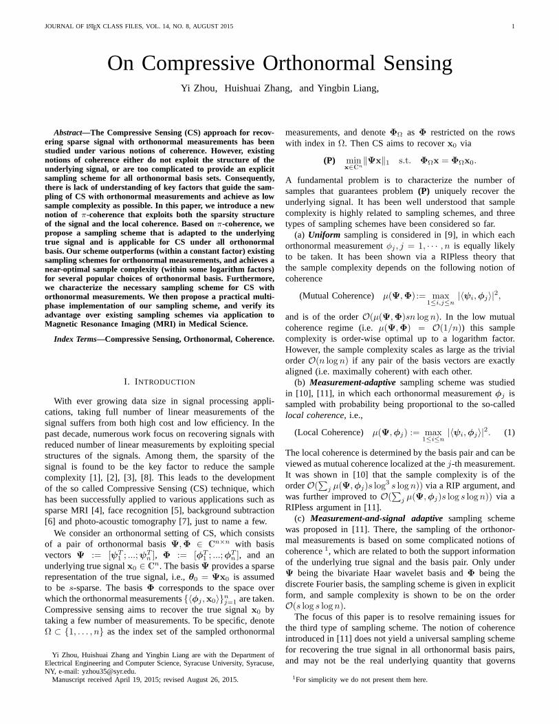
We first consider the noisefree setting, and apply thesampling schemes of interest to recover a 256×256 MRIbrain image. The budget of measurements is set to be20%, 25%, · · · , 70% of the total dimensions, respectively. ThenumberP of phases for the multi-phase sampling schemes isset to be two, which is justified in our subsequent experimentin Section V-B. Denotex∗ as the original image andx asthe recovered image. We report the relative error‖x∗−x‖2

‖x∗‖2.


Figure 1 plots how the relative error reduces as the total budgetincreases for four sampling schemes. It can be seen that theuniform sampling [8] and the uniform by level scheme [11]suffer from high relative error and instability, while the basis-adaptive scheme in [10] and our scheme provide more accurateand stable recovery. In particular, our scheme outperformsall other three schemes. It is superior over the uniform andbasis adaptive sampling due to the fact that it adapts toboth the local coherence of basis and the signal spaceΠ.Although the uniform by level sampling also adapts to thesignal information, adaption is limited only across levels, notover the entire basis vectors as in our scheme.

Fig. 1. Comparison of relative errors of four sampling schemes to recover amedical image as the number of measurements increases.

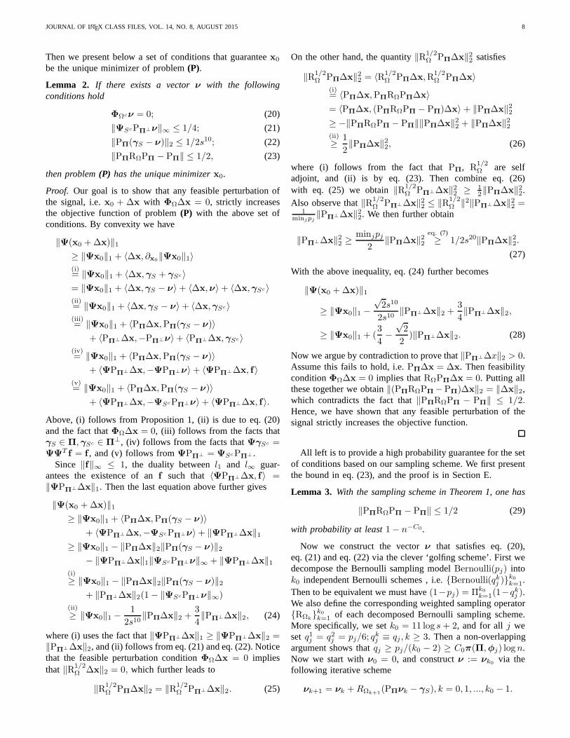
To provide a better illustration, we present in Figure 2the recovered images and their corresponding sampling masksof the sampled Fourier frequencies for the setting with30%budget of total dimensions.

One can see that the image recovered by our samplingscheme has the best quality. Note that we have shifted theFourier basis to center the spectrum and the sampling masks.One can see that the sampling mask of the uniform by levelscheme in [11] has a block structure, which does not fit thespectrum of the original signal well. The sampling mask ofthe basis-adaptive scheme in [10] is a good approximationof the spectrum of practical smooth images, but is generatedby a fixed probability distribution that is not adapted to theunderlying signal. Our sampling mask is the mixture of auniform mask (in the initial phase) and a mask generated byadaptive sampling scheme (in the second phase). Despite itsuniform part of the mask, one can see that the mask of ourscheme is well adapted to the spectrum of the original signal.

B. Number of Phases

A key parameter that affects multi-phase sampling schemesis the numberP of phases. Intuitively, largerP allows moremeasurements to be sampled adaptively, but requires morecomputation for estimatingΠ,Π⊥ and pj in each phase.Hence, a good choice ofP can well balance the recovery errorand computational load. We apply our multi-phase samplingscheme with30% measurements of the total dimensions to

Number of phase 2 3 4 5Relative Error 0.095 0.085 0.089 0.082

TABLE ICOMPARISON OF THE PERFORMANCE OF OUR MULTI-PHASE SAMPLING

SCHEME UNDER DIFFERENT NUMBERS OF PHASES

recover an MRI image, and set the number of phases to beP = 2, · · · , 5, respectively. Table I shows the relationshipbetween the number of phases and the corresponding relativeerror. One can see that for more than 2 phases the relativeerror stays at the same level. This suggests that two phasesare sufficiently good to achieve a low relative error for ourexperiments.

VI. CONCLUSION

We propose a Bernoulli sampling scheme for CS withorthonormal basis, which is applicable to all orthonormal basispairs. The scheme is based onπ-coherence that exploits boththe support structure of the signal and the local coherence.Our sampling scheme reveals the relationship between samplecomplexity and sparsity of the signal as well as coherencepattern of the basis, and achieves lower sample complexity(within a constant factor) than that of existing basis and signaladaptive sampling schemes. Furthermore, we characterize theneccessary sampling scheme for orthonormal measurements.We also propose a practical multi-phase implementation of oursampling scheme, and demonstrate its advantage over otherexisting sampling schemes via experiments. We anticipate thatsuch signal-dependent adaptive sampling together with multi-phase implementation can be useful for other high dimensionalproblems with limited budget of measurements.

REFERENCES

[1] D. Donoho, “Compressed sensing,”IEEE Transactions on InformationTheory, vol. 52, pp. 1289–1306, 2006.

[2] E. Candes and T. Tao, “Near-optimal signal recovery from randomprojections: Universal encoding strategies?”IEEE Transactions on In-formation Theory, vol. 52, no. 12, pp. 5406–5425, 2006.

[3] E. Candes, J. Romberg, and T. Tao, “Stable signal recovery fromincomplete and inaccurate measurements,”Communications on Pure andApplied Mathematics, vol. 59, no. 8, pp. 1207–1223, 2006.

[4] M. Lustig, D. Donoho, J. Santos, and J. Pauly, “Compressed sensingmri,” in IEEE Signal Processing Magazine, 2007.

[5] J. Wright, A. Yang, A. Ganesh, S. Sastry, and Y. Ma, “Robust facerecognition via sparse representation,”IEEE Transactions on PatternAnalysis and Machine Intelligence, vol. 31, no. 2, pp. 210–227, 2009.

[6] V. Cevher, A. Sankaranarayanan, M. Duarte, D. Reddy, andR. Bara-niuk, “Compressive sensing for background subtraction,” in EuropeanConference on Computer Vision, 2008, pp. 155–168.

[7] J. Provost and F. Lesage, “The application of compressedsensing forphoto-acoustic tomography,”IEEE Transactions on Medical Imaging,vol. 28, no. 4, pp. 585–594, 2009.

[8] E. Candes and Y. Plan, “A probabilistic and ripless theory of compressedsensing,”IEEE Transactions on Information Theory, vol. 57, no. 11, pp.7235–7254, 2011.

[9] E. Candes and J. Romberg, “Sparsity and incoherence in compressivesampling,” Inverse Problems, vol. 23, no. 3, p. 969, 2007.

[10] F. Krahmer and R. Ward, “Stable and robust sampling strategies forcompressive imaging,”IEEE Transactions on Image Processing, vol. 23,no. 2, pp. 612–622, 2014.

[11] C. Boyer, J. Bigot, and P. Weiss, “Compressed sensing with structuredsparsity and structured acquisition,”arxiv, 2015.

[12] Z. Wang and G. Arce, “Variable density compressed imagesampling,”IEEE Transactions on Image Processing, vol. 19, no. 1, pp. 264–270,2010.


Fig. 2. Comparison of recovered images and sampling masks offour sampling schemes with 30% measurements of total dimensions.

[13] C. Schroder, P. Bornert, and B. Aldefeld, “Spatial excitation usingvariable-density spiral trajectories,”Journal of Magnetic ResonanceImaging, vol. 18, no. 1, pp. 136–141, 2003.

[14] G. Puy, J. Marques, R. Gruetter, J. Thiran, D. Ville, P. Vandergheynst,and Y. Wiaux, “Spread spectrum magnetic resonance imaging,” arxiv,2012.

[15] N. Chauffert, P. Ciuciu, and P. Weiss, “Variable Density CompressedSensing In MRI. Theoretical vs Heuristic Sampling Strategies,” inInternational Symposium on Biomedical Imaging, 2013.

[16] B. Adcock, P. Univ, A. Hansen, C. Poon, and B. Roman, “Breakingthe coherence barrier: asymptotic incoherence and asymptotic sparsityin compressed sensing,” Tech. Rep., 2013.

[17] L. Malloy and D. Nowak, “Near-optimal adaptive compressed sensing,”IEEE Transactions on Information Theory, vol. 60, no. 7, pp. 4001–4012, 2013.

[18] M. Iwen and A. H. Tewfik, “Adaptive compressed sensing for sparsesignals in noise,” inConference on Circuits, Systems & Computers, 2011,pp. 1240–1244.

[19] J. Haupt, R. Baraniuk, R. Castro, and R. Nowak, “Sequentially designedcompressed sensing,” inIEEE Statistical Signal Processing Workshop,2012, 2012, pp. 401–404.

[20] C. Boutsidis, M. Mahoney, and P. Drineas, “An improved approxima-tion algorithm for the column subset selection problem,”ComputingResearch Repository, vol. abs/0812.4, 2008.

[21] M. Mahoney, “Randomized algorithms for matrices and data,” Comput-ing Research Repository, 2011.

[22] Y. Chen, S. Bhojanapalli, S. Sanghavi, and R. Ward, “Coherent matrixcompletion,” in Proceedings of the 31st International Conference onMachine Learning, 2014, pp. 674–682.

[23] H. Rauhut, “Compressive sensing and structured randommatrices,”Radon Series Comp. Appl. Math, 2010.

[24] D. Gross, “Recovering low-rank matrices from few coefficients in anybasis,” IEEE Transactions on Information Theory, vol. 57, no. 3, pp.1548–1566, 2011.

[25] Y. Chen, “Completing any low-rank matrix, provably,”arxiv, 2013.[26] H. Zhang, Y. Liang, and Y. Zhou, “Analysis of robust pca via local

incoherence,”NIPS, 2015.[27] E. Candes, J. Romberg, and T. Tao, “Robust uncertaintyprinciples: exact

signal reconstruction from highly incomplete frequency information,”IEEE Transactions on Information Theory, vol. 52, no. 2, pp. 489–509,Feb 2006.

[28] M. Guerquin-Kern, M. Haberlin, K. Pruessmann, and M. Unser, “A fastwavelet-based reconstruction method for magnetic resonance imaging,”IEEE Transactions on Medical Imaging, vol. 30, no. 9, pp. 1649–1660,Sept 2011.

APPENDIX APROOF OFTHEOREM 1

We first characterize the sub-differential of‖Ψx0‖1 via thefollowing proposition for convenience.

Proposition 1. The sub-differential of‖Ψx0‖1 w.r.t. x0 canbe expressed as∂x0

‖Ψx0‖1 = γS + γSc , where

γS =∑

j∈S

sgn(θ)jψj , γSc :=

∑

j∈Sc

fjψj | ‖f‖∞ ≤ 1

.

Moreover,γS ∈ Π andγSc ∈ Π⊥.

Proof. Consider arbitrary vectorx with its support set denotedasS, it is well known that

∂‖x‖1 := sgn(x) + f | supp(f) = Sc, ‖f‖∞ ≤ 1.. (16)

Then for the vectorθ = Ψx0 with support setS, the chainrule gives

∂x0‖Ψx0‖1 = Ψ

T ∂‖Ψx0‖1 (17)(i)= Ψ

T (sgn(θ) + f) (18)(ii)=∑

j∈S

sgn(θ)jψj

︸︷︷︸

γS

+∑

j∈Sc

fjψj

︸︷︷︸

γSc

, (19)

where (i) follows from the sub-differential in eq. (16), and(ii) follows from the fact thatsupp(θ) = S, supp(f) = Sc.Clearly,γS ∈ Π,γSc ∈ Π

⊥.

Next we introduce the random variableδj ∼ Bernoulli(pj),and define the weighted sampling operators

RΩ(x) :=

n∑

j=1

δjpj〈x, φj〉φj ,R

1/2Ω (x) =

n∑

j=1

δj√pj〈x,φj〉φj .


Then we present below a set of conditions that guaranteex0

be the unique minimizer of problem(P).

Lemma 2. If there exists a vectorν with the followingconditions hold

ΦΩcν = 0; (20)

‖ΨScPΠ⊥ν‖∞ ≤ 1/4; (21)

‖PΠ(γS − ν)‖2 ≤ 1/2s10; (22)

‖PΠRΩPΠ − PΠ‖ ≤ 1/2, (23)

then problem(P) has the unique minimizerx0.

Proof. Our goal is to show that any feasible perturbation ofthe signal, i.e.x0 + ∆x with ΦΩ∆x = 0, strictly increasesthe objective function of problem(P) with the above set ofconditions. By convexity we have

‖Ψ(x0 +∆x)‖1≥ ‖Ψx0‖1 + 〈∆x, ∂x0

‖Ψx0‖1〉(i)= ‖Ψx0‖1 + 〈∆x,γS + γSc〉= ‖Ψx0‖1 + 〈∆x,γS − ν〉+ 〈∆x,ν〉+ 〈∆x,γSc〉(ii)= ‖Ψx0‖1 + 〈∆x,γS − ν〉+ 〈∆x,γSc〉(iii)= ‖Ψx0‖1 + 〈PΠ∆x,PΠ(γS − ν)〉

+ 〈PΠ⊥∆x,−PΠ⊥ν〉+ 〈PΠ⊥∆x,γSc〉(iv)= ‖Ψx0‖1 + 〈PΠ∆x,PΠ(γS − ν)〉

+ 〈ΨPΠ⊥∆x,−ΨPΠ⊥ν〉+ 〈ΨPΠ⊥∆x, f〉(v)= ‖Ψx0‖1 + 〈PΠ∆x,PΠ(γS − ν)〉

+ 〈ΨPΠ⊥∆x,−ΨScPΠ⊥ν〉+ 〈ΨPΠ⊥∆x, f〉.

Above, (i) follows from Proposition 1, (ii) is due to eq. (20)and the fact thatΦΩ∆x = 0, (iii) follows from the facts thatγS ∈ Π,γSc ∈ Π

⊥, (iv) follows from the facts thatΨγSc =ΨΨ

Tf = f , and (v) follows fromΨPΠ⊥ = ΨScPΠ⊥ .

Since ‖f‖∞ ≤ 1, the duality betweenl1 and l∞ guar-antees the existence of anf such that 〈ΨPΠ⊥∆x, f〉 =‖ΨPΠ⊥∆x‖1. Then the last equation above further gives

‖Ψ(x0 +∆x)‖1≥ ‖Ψx0‖1 + 〈PΠ∆x,PΠ(γS − ν)〉

+ 〈ΨPΠ⊥∆x,−ΨScPΠ⊥ν〉+ ‖ΨPΠ⊥∆x‖1≥ ‖Ψx0‖1 − ‖PΠ∆x‖2‖PΠ(γS − ν)‖2− ‖ΨPΠ⊥∆x‖1‖ΨScPΠ⊥ν‖∞ + ‖ΨPΠ⊥∆x‖1

(i)

≥ ‖Ψx0‖1 − ‖PΠ∆x‖2‖PΠ(γS − ν)‖2+ ‖PΠ⊥∆x‖2(1− ‖ΨScPΠ⊥ν‖∞)

(ii)

≥ ‖Ψx0‖1 −1

2s10‖PΠ∆x‖2 +

3

4‖PΠ⊥∆x‖2, (24)

where (i) uses the fact that‖ΨPΠ⊥∆x‖1 ≥ ‖ΨPΠ⊥∆x‖2 =‖PΠ⊥∆x‖2, and (ii) follows from eq. (21) and eq. (22). Noticethat the feasible perturbation conditionΦΩ∆x = 0 impliesthat ‖R1/2

Ω ∆x‖2 = 0, which further leads to

‖R1/2Ω PΠ∆x‖2 = ‖R1/2

Ω PΠ⊥∆x‖2. (25)

On the other hand, the quantity‖R1/2Ω PΠ∆x‖22 satisfies

‖R1/2Ω PΠ∆x‖22 = 〈R1/2

Ω PΠ∆x,R1/2Ω PΠ∆x〉

(i)= 〈PΠ∆x,PΠRΩPΠ∆x〉= 〈PΠ∆x, (PΠRΩPΠ − PΠ)∆x〉 + ‖PΠ∆x‖22≥ −‖PΠRΩPΠ − PΠ‖‖PΠ∆x‖22 + ‖PΠ∆x‖22(ii)

≥ 1

2‖PΠ∆x‖22, (26)

where (i) follows from the fact thatPΠ, R1/2Ω are self

adjoint, and (ii) is by eq. (23). Then combine eq. (26)with eq. (25) we obtain‖R1/2

Ω PΠ⊥∆x‖22 ≥ 12‖PΠ∆x‖22.

Also observe that‖R1/2Ω PΠ⊥∆x‖22 ≤ ‖R

1/2Ω ‖2‖PΠ⊥∆x‖22 =

1minjpj

‖PΠ⊥∆x‖22. We then further obtain

‖PΠ⊥∆x‖22 ≥minjpj

2‖PΠ∆x‖22

eq. (7)≥ 1/2s20‖PΠ∆x‖22.

(27)

With the above inequality, eq. (24) further becomes

‖Ψ(x0 +∆x)‖1

≥ ‖Ψx0‖1 −√2s10

2s10‖PΠ⊥∆x‖2 +

3

4‖PΠ⊥∆x‖2,

≥ ‖Ψx0‖1 + (3

4−√2

2)‖PΠ⊥∆x‖2. (28)

Now we argue by contradiction to prove that‖PΠ⊥∆x‖2 > 0.Assume this fails to hold, i.e.PΠ∆x = ∆x. Then feasibilityconditionΦΩ∆x = 0 implies thatRΩPΠ∆x = 0. Putting allthese together we obtain‖(PΠRΩPΠ−PΠ)∆x‖2 = ‖∆x‖2,which contradicts the fact that‖PΠRΩPΠ − PΠ‖ ≤ 1/2.Hence, we have shown that any feasible perturbation of thesignal strictly increases the objective function.

All left is to provide a high probability guarantee for the setof conditions based on our sampling scheme. We first presentthe bound in eq. (23), and the proof is in Section E.

Lemma 3. With the sampling scheme in Theorem 1, one has

‖PΠRΩPΠ − PΠ‖ ≤ 1/2 (29)

with probability at least1− n−C0 .

Now we construct the vectorν that satisfies eq. (20),eq. (21) and eq. (22) via the clever ‘golfing scheme’. First wedecompose the Bernoulli sampling modelBernoulli(pj) intok0 independent Bernoulli schemes , i.e.Bernoulli(qkj )k0

k=1.Then to be equivalent we must have(1−pj) = Πk0

k=1(1−qkj ).We also define the corresponding weighted sampling operatorRΩk

k0

k=1 of each decomposed Bernoulli sampling scheme.More specifically, we setk0 = 11 log s+ 2, and for allj weset q1j = q2j = pj/6; q

kj ≡ qj , k ≥ 3. Then a non-overlapping

argument shows thatqj ≥ pj/(k0 − 2) ≥ C0π(Π,φj) logn.Now we start withν0 = 0, and constructν := νk0

via thefollowing iterative scheme

νk+1 = νk +RΩk+1(PΠνk − γS), k = 0, 1, ..., k0 − 1.


By introducing the variablesw0 = −γS , wk = PΠνk − γS ,the above iterative scheme can be expressed as

νk0=

k0∑

k=1

RΩkwk−1, (30)

wk = (PΠRΩkPΠ − PΠ)wk−1, k = 1, ..., k0, (31)

which brings more convenience for subsequent analysis. Be-fore proving the conditions on the constructedνk0

, we firstcollect the following concentration bound for convenience.The proof is in Section F.

Lemma 4. For any vectorw, one has

‖(PΠRΩkPΠ − PΠ)w‖2 ≤

1

2‖w‖2, k = 1, 2..., k0 (32)


Also, note that the infinity norm induced by basisΦ ismaxj |[Φw]j | = maxj |〈w,φj〉|. By scaling this norm withthe scalar‖PΠφj‖2, we then define the following weightednorm ‖ · ‖Φ,∞

‖w‖Φ,∞ := maxj

|〈w,φj〉|‖PΠφj‖2

.

Equipped with this weighted norm, the following boundsholds. The proof are in Section G, Section H, and Section I,respectively.

Lemma 5. For any vectorw, one has

‖ΨSc(RΩk− I)w‖∞ ≤

1√C0

‖w‖Φ,∞, k = 1, 2...k0

with probability at least1− n−√C0 .

Lemma 6. For any vectorw ∈ Π, one has

‖(PΠRΩkPΠ − PΠ)w‖Φ,∞≤

‖w‖Φ,∞/

√log s, k ∈ 1, 2

‖w‖Φ,∞/2, k = 3, 4..., k0


Lemma 7. With probability at least1− s−√C0/4, one has

‖γS‖Φ,∞ ≤√C0 log s

4. (33)

Now equipped with all technical lemmas above, we showthat the constructedνk0

satisfies the set of conditions. First, bythe decomposition of the Bernoulli sampling model, eq. (30)directly implies eq. (21). Next we verify eq. (22) via

‖PΠ(γS − νk0)‖2 = ‖wk0

‖2(eq. (31))= ‖(PΠRΩk0

PΠ − PΠ)wk0−1‖2

(Lemma 4)≤ 1

2‖wk0−1‖2 ≤ ... ≤ 1

211 log s+2‖γS‖2

≤√s

4s11≤ 1

2s10.

Finally, we verify eq. (21) via

‖ΨScPΠ⊥νk0‖∞ = ‖ΨSc

k0∑

k=1

PΠ⊥RΩkwk−1‖∞

(wk ∈ Π) = ‖ΨSc

k0∑

k=1

PΠ⊥(RΩk− I)wk−1‖∞

(triangle inequality)≤k0∑

k=1

‖ΨScPΠ⊥(RΩk− I)wk−1‖∞

(ΨScPΠ = 0) =k0∑

k=1

‖ΨSc(RΩk− I)wk−1‖∞

(Lemma 5)≤k0∑

k=1

1√C0

‖wk−1‖Φ,∞

(Lemma 6)≤k0∑

k=1

1√C0

1

log s

1

2k−1‖w0‖Φ,∞

(w0 = −γS) ≤ ‖γS‖Φ,∞√C0 log s

(Lemma 7)≤ 1

4.

To this end we have shown that the constructedνk0satisfies

all conditions, and the succeed probability over all the proofis dominated by1− s−

√C0/4.

APPENDIX BPROOF OFTHEOREM 2

Let’s prove the first inequality. For the two terms involvedin π coherence, we have

‖PΠφj‖22 = 〈ΨPΠφj ,ΨPΠφj〉(dual norm)≤ ‖ΨPΠφj‖1‖ΨPΠφj‖∞

≤ ‖ΨPΠφj‖1‖Ψφj‖∞= ‖ΨPΠφj‖1

√

µ(Ψ,φj),

and

‖PΠφj‖2‖ΨPΠ⊥φj‖∞ ≤ ‖ΨPΠφj‖2‖Ψφj‖∞(l2 ≤ l1) ≤ ‖ΨPΠφj‖1‖Ψφj‖∞

= ‖ΨPΠφj‖1√

µ(Ψ,φj).

Hence, the first inequality holds. For the second inequality, webegin with

‖ΨPΠφj‖1√

µ(Ψ,φj) = ‖ΨPΠφj‖1‖Ψφj‖∞(dim(Π) = s) ≤ s‖ΨPΠφj‖∞‖Ψφj‖∞

≤ s‖Ψφj‖2∞= sµ(Ψ,φj).

Now the third inequality holds trivially.The sampling scheme in [10] has sample complexity of the

orderO(∑j µ(Ψ,φj)s log3 s logn), while ours is of the order

O(∑j π(Π,φj) log s logn). Thus, by the second inequalityour sample complexity is lower. The sample complexity in[11] is of the orderO(maxΘ,Γ log s logn), whereΘ,Γ are


two complicated notions of coherence that both depend on thesampling probability. There’s no general closed form for theoptimal sampling scheme that minimizes the two coherences.However, we can consider the lower boundO(Θ log s logn),which can be minimized by the sampling scheme

pj ∝‖ΨPΠφj‖1

√µ(Ψ,φj)

∑

j ‖ΨPΠφj‖1√µ(Ψ,φj)

(34)

with complexity O(∑j ‖ΨPΠφj‖1√µ(Ψ,φj) log s logn).

Hence by our first inequality, our sample complexity is lower.

APPENDIX CPROOF OFLEMMA 1

Adopt the definition of local coherence, we define

‖ΨPΠlφj‖∞ =

√

µ(Πl,φj) (35)

‖ΨPΠ⊥φj‖∞ =√

µ(Π⊥,φj). (36)

Sincedim(Πl) = sl, we obtain by the relationship betweenl2 and l∞ that

‖PΠlφj‖22 ≤ sl‖ΨPΠl

φj‖2∞eq. (35)= slµ(Πl,φj). (37)

Thus, we obtain the upper bound

‖PΠφj‖2‖ΨPΠ⊥φj‖∞ (38)

(eq. (3), eq. (36))=

√√√√

p∑

l=1

‖PΠlφj‖22

√

µ(Π⊥,φj) (39)

(eq. (37))≤

√√√√

p∑

l=1

slµ(Πl,φj)µ(Π⊥,φj). (40)

Next we decomposeΠ w.r.t. different dyadic levels. Specif-ically, we denoteΠl : Π ∩ spanψj | j ∈ Ll, i.e. the partof Π in the subspace spanned by the wavelet basis in levell,and it follows thatΠ =

⊕pl=0 Πl. Now we have

n∑

j=1

‖PΠφj‖2‖ΨPΠ⊥φj‖∞

(eq. (40))≤n∑

j=1

√√√√

p∑

l=0

slµ(Πl,φj)µ(Π⊥,φj)

≤n∑

j=1

√√√√

p∑

l=0

slµ(Πl,φj)µ(Ψ,φj)

≤n∑

j=1

√√√√

p∑

l=0

sl maxi∈Ll

µ(ψi,φj)maxi

µ(ψi,φj)

(eq. (11))≤n∑

j=1

√√√√

p∑

l=0

sl2−k(j)2−|k(j)−l|2−k(j)

≤n∑

j=1

p∑

l=0

√sl2

−k(j)2−|k(j)−l|/2

(|Lk(j)| ≤ 2k(j)) ≤p∑

l=0

√sl

p∑

k(j)=0

2−|k(j)−l|/2

≤ 2√2√

2− 1

p∑

l=0

√sl

≤ 2√2√

2− 1s.

Since we have shown that∑n

j=1 ‖PΠφj‖22 = s, the over-all sample complexity of eq. (6) is upper bounded byO(s log s logn).

APPENDIX DPROOF OFTHEOREM 3

Let us introduce the Bernoulli random variablesδj Bernoulli(pj), j = 1, · · · , n, and the number of sampledmeasurements can be represented by|Ω| = ∑n

j=1 δj . Thenthe converse scheme in eq. (14) implies that

E|Ω| =n∑

j=1

pj ≤n∑

j=1

‖PΠφj‖22 ≤ s. (41)

Hence, a simple Hoeffding’s bound gives that|Ω| < s−2 withhigh probability.

Now let us identify a set of candidatesx that achieves thesame objective value asx0. Recall thatθ := Ψx0 with supportsetS, and our constructedx is as follows

x := x0 −ΨT (λ · sgn(θ)), where |λ| 4 |θ|. (42)

In the above expression,λ is a vector, ‘·’ denotes the element-wise product, and ‘4’ means≤ holds element-wise. Conse-quently, the objective value of problem(P) for x becomes

‖Ψx‖1 = ‖θ − λ · sgn(θ)‖1=∑

i∈S

|θi − λisgn(θi)|

(i)=∑

i∈S

|θi| − λi

= ‖Ψx0‖1 − 〈λ,1S〉,where (i) follows from |λ| 4 |θ|, and 1S denotes a vectorthat has 1s on the support setS. Thus, to achieve the sameobjective value we only need to require

〈λ,1S〉 = 0. (43)

Moreover, the linear constraint of problem(P) requiresΦΩx =ΦΩx0. Then with the form ofx, this constraint becomes

ΦΩΨT (λ · sgn(θ)) = 0. (44)

Notice from eqs. (43) and (44) that we only need to identifythe entries ofλ that are supported onS, and the total numberof linear constrains are1+ |Ω| < s− 1. Thus, we can identifyinfinite manyλs that satisfy eqs. (43) and (44). Finally, toensure that|λ| 4 |θ| we simply apply the normalization

∀i ∈ S, λi ← λimini |θi|‖λ‖∞

. (45)


APPENDIX EPROOF OFLEMMA 3

The operator can be equivalently expressed as:

(PΠRΩPΠ − PΠ)(·) =n∑

j=1

(δjpj− 1

)

〈φj ,PΠ(·)〉PΠφj

def=

n∑

j=1

Xj(·).

Then for each operatorXj(·), its operator norm can bebounded as

‖Xj(·)‖ = maxz

‖Xj(z)‖2‖z‖2

≤ maxz

‖PΠφj‖22‖z‖2pj‖z‖2

eq. (6)≤ 1

C0 logn.

Moreover, the operator norm of its variance‖∑n

j=1 EX 2j (·)‖

can be bounded as∥∥∥∥∥∥

n∑

j=1

EX 2j (·)

∥∥∥∥∥∥

= maxz

‖∑nj=1 EX 2

j (z)‖2‖z‖2

= maxz

∥∥∥∥∥∥

n∑

j=1

E

(δjpj− 1

)2

〈φj ,PΠz〉〈φj ,PΠφj〉PΠφj

∥∥∥∥∥∥2

/‖z‖2

= maxz

∥∥∥∥∥∥

n∑

j=1

(1− pj)‖PΠφj‖22pj

〈φj ,PΠz〉PΠφj

∥∥∥∥∥∥2

/‖z‖2

≤ maxz

maxj

(1− pj)‖PΠφj‖22pj

∥∥∥∥∥∥

n∑

j=1

〈φj ,PΠz〉φj

∥∥∥∥∥∥2

/‖z‖2

≤ maxz

maxj

‖PΠφj‖22pj

‖PΠz‖2‖z‖2

(i)

≤ 1

C0 logn,

where (i) follows from eq. (6). Then apply the matrix Bern-stein’s inequality in Theorem 6 gives the result.

APPENDIX FPROOF OFLEMMA 4

For all k = 1, · · · , k0, we expand(PΠRΩkPΠ − PΠ)w as

(PΠRΩkPΠ − PΠ)w =

n∑

j=1

(

δkj

qkj− 1

)

〈φj ,PΠw〉PΠφj

def=

n∑

j=1

X kj .

Then for allj we have

‖X kj ‖2 =

∥∥∥∥∥

(

δkjqkj− 1

)

〈PΠφj ,w〉PΠφj

∥∥∥∥∥2

≤ ‖PΠφj‖22qkj

‖w‖2

(i)

≤ ‖w‖2C0 logn

, k = 1, 2...k0

where (i) is by the specification ofqkj of the golfing scheme.Moreover, for the variance part we have

n∑

j=1

E‖X kj ‖22 =

n∑

j=1

E

(

δkj

qkj− 1

)2

|〈φj ,PΠw〉|2‖PΠφj‖22

≤n∑

j=1

‖PΠφj‖22qkj

|〈φj ,PΠw〉|2

≤ maxj

(

‖PΠφj‖22qkj

)

‖PΠw‖22

(i)

≤ ‖w‖22C0 logn

, k = 1, 2...k0

where (i) also follows from the specification ofqkj of thegolfing scheme. The result follows from the vector Bernstein’sinequality in Theorem 5.

APPENDIX GPROOF OFLEMMA 5

SinceΨSc is restricted on the rowsψTi , i ∈ Sc, ΨSc(RΩk

−I)w is thus supported onSc. The i-th entry inSc of vectorΨSc(RΩk

− I)w can be alternatively expressed as

[ΨSc(RΩk− I)w]i =

n∑

j=1

(

δkj

qkj− 1

)

〈φj ,w〉〈φj ,ψi〉

def=

n∑

j=1

X kj , i ∈ Sc.

By the specifications of the golfing scheme, we have for allkthat qkj ≥ C0‖PΠφj‖2‖ΨPΠ⊥φj‖∞ log n. We then obtain

|X kj | =

∣∣∣∣∣

(

δkjqkj− 1

)

〈φj ,w〉〈φj ,ψi〉∣∣∣∣∣

≤∣∣∣∣

〈φj ,w〉〈φj ,ψi〉C0‖PΠφj‖2‖ΨPΠ⊥φj‖∞ logn

∣∣∣∣

(i)

≤ ‖w‖Φ,∞C0 logn

,

where (i) follows from the fact that |〈φj ,ψi〉| ≤‖ΨPΠ⊥φj‖∞ for all i ∈ Sc. Moreover, we also haveqkj ≥ C0‖PΠφj‖22 logn. Then we obtain

n∑

j=1

E|X kj |2 =

n∑

j=1

E

(

δkj

qkj− 1

)2

|〈φj ,w〉〈φj ,ψi〉|2

≤n∑

j=1

|〈φj ,w〉〈φj ,ψi〉|2

qkj

≤ maxj

|〈φj ,w〉|2qkj

n∑

j=1

|〈φj ,ψi〉|2

≤ maxj

|〈φj ,w〉|2C0‖PΠφj‖22 logn

≤‖w‖2

Φ,∞C0 logn

.

The result follows from scalar Bernstein’s inequality in The-orem 4 and a union bound.


APPENDIX HPROOF OFLEMMA 6

By the definition of the weighted norm, we have

‖(PΠRΩkPΠ − PΠ)w‖Φ,∞ = max

j

|〈(PΠRΩkPΠ − PΠ)w,φj〉|‖PΠφj‖2

= maxj

∣∣∣∣∣∣

∑ni=1

(δkiqki− 1)

〈φi,PΠw〉〈PΠφi,φj〉‖PΠφj‖2

∣∣∣∣∣∣

.

Now consider thej-th term, i.e.,∣∣∣∣∣∣

n∑

i=1

(δkiqki

− 1)


∣∣∣∣∣∣

def= |

n∑

i=1

X ki |

we have that

|X ki | =

∣∣∣∣∣∣

(δkiqki

− 1)


∣∣∣∣∣∣

(i)

≤∣∣∣∣

〈φi,w〉‖PΠφi‖2qki

∣∣∣∣

≤

[C0 logn log s]−1 ‖w‖Φ,∞, k ∈ 1, 2

[C0 logn]−1 ‖w‖Φ,∞, k = 3, 4...k0

where (i) follows from Cauchy-Swartz and the fact thatw ∈Π. Moreover, we have

n∑

i=1

E|X ki |2

=

n∑

i=1

E

(δkiqki− 1

)2 ∣∣∣∣

|〈φi,PΠw〉|2|〈PΠφi,φj〉|2‖PΠφj‖22

∣∣∣∣

≤ 1

‖PΠφj‖22

n∑

i=1

∣∣∣∣

|〈φi,PΠw〉|2|〈φi,PΠφj〉|2qki

∣∣∣∣

(i)

≤ maxi

|〈φi,w〉|2qki

1

‖PΠφj‖22

n∑

i=1

|〈φi,PΠφj〉|2

= maxi

|〈φi,w〉|2qki

(ii)

≤

[C0 logn log s]−1 ‖w‖2

Φ,∞, k ∈ 1, 2[C0 logn]

−1 ‖w‖2Φ,∞, k = 3, 4...k0

where (i) follows from the fact thatw ∈ Π, and (ii) utilizes thespecifications ofqki of the golfing scheme. The result followsfrom the scalar Bernstein’s inequality in Theorem 4 and aunion bound.

APPENDIX IPROOF OFLEMMA 7

Recall thatγS =∑

i∈S sgn(θ)iψi, and by definition

‖γS‖Φ,∞ = maxj

|〈φj ,γS〉|‖PΠφj‖2

= maxj

|∑

i∈S sgn(θ)i〈φj ,ψi〉|‖PΠφj‖2

def= max

j

|∑i∈S Xi|‖PΠφj‖2

.

Now for for eachj we bound the term|∑i∈S Xi|. We have

|Xi| = |sgn(θ)i〈φj ,ψi〉| ≤ ‖PΠφj‖2

=

√C0‖PΠφj‖2 log s/4√

C0 log s/4,

where we have used the fact thatψi ∈ Π for i ∈ S. Moreover,we have forC0 > 1

∑

i∈S

E|Xi|2 ≤∑

i∈S

|〈φj ,ψi〉|2 = ‖PΠφj‖22

≤ C0‖PΠφj‖22 log2 s/16√C0 log s/4

.

Then scalar Bernstein’s inequality in Theorem 4 and a unionbound gives the result.

APPENDIX JBERNSTEIN’ S INEQUALITIES

Theorem 4 (Scalar Bernstein’s inequality). Let x1, · · · , xm ∈R be independent, zero mean random variables. If for alli =1, · · · ,m, it holds that|xi| ≤ B and

∑mi=1 E|xi|2 ≤ σ2, then

P

(∣∣∣∣∣

m∑

i=1

xi

∣∣∣∣∣> t

)

≤ 2exp

(

− t2/2

σ2 +Bt/3

)

. (46)

Theorem 5 (Vector Bernstein’s inequality). Letx1, · · · ,xm ∈Rn be independent, zero mean random vectors. If for alli =1, · · · ,m, it holds that‖xi‖2 ≤ B and

∑mi=1 E‖xi‖22 ≤ σ2,

then for all 0 < t < σ2/B

P

(∥∥∥∥∥

m∑

i=1

xi

∥∥∥∥∥2

> t

)

≤ exp

(

− t2

8σ2+

1

4

)

. (47)

Theorem 6 (Matrix Bernstein’s inequality). LetX1, · · · ,Xm ∈ R

n×n be independent, zero mean randommatrices. If for alli = 1, · · · ,m, it holds that‖Xi‖ ≤ B andmax‖∑m

i=1 EXTi Xi‖, ‖

∑mi=1 EXiX

Ti ‖ ≤ σ2, then for all

c > 0∥∥∥∥∥

m∑

i=1

Xi

∥∥∥∥∥≤ 2√

cσ2log2n+ cBlog2n (48)

with probability at least1− 2n−(c−1).

JOURNAL OF LA On Compressive Orthonormal Sensing - Yingbin Liang's...

Documents

Transcript of JOURNAL OF LA On Compressive Orthonormal Sensing - Yingbin Liang's...