Journal of Hydrology - WaterUse... · The economic impact of more sustainable water use in...

Journal of Hydrology 384 (2010) 292–305

Contents lists available at ScienceDirect

Journal of Hydrology

journal homepage: www.elsevier .com/locate / jhydrol

The economic impact of more sustainable water use in agriculture:A computable general equilibrium analysis

Alvaro Calzadilla a,b,*, Katrin Rehdanz a,c,d, Richard S.J. Tol e,f,g

a Research unit Sustainability and Global Change, Hamburg University and Centre for Marine and Atmospheric Science, Bundesstraße 55, 20146 Hamburg, Germanyb International Max Planck Research School on Earth System Modelling, Bundesstraße 53, 20146 Hamburg, Germanyc Christian-Albrechts-University of Kiel, Department of Economics, Olshausenstraße 40, 24118 Kiel, Germanyd Kiel Institute for the World Economy, Duesternbrooker Weg 120, 24105 Kiel, Germanye Economic and Social Research Institute, Whitaker Square Sir John Rogerson’s Quay, Dublin 2, Irelandf Institute for Environmental Studies, Vrije Universiteit, De Boelelaan 1087, 1081 HV Amsterdam, The Netherlandsg Department of Spatial Economics, Vrije Universiteit, De Boelelaan 1105, 1081 HV Amsterdam, The Netherlands

a r t i c l e i n f o s u m m a r y

JEL classification:Q17D58Q15Q25

Keywords:Agricultural water useComputable general equilibriumIrrigationSustainable water use

0022-1694/$ - see front matter � 2009 Elsevier B.V. Adoi:10.1016/j.jhydrol.2009.12.012

* Corresponding author. Present address: ResearchChange, Hamburg University and Centre for MarinBundesstrasse 55 (Pavillion Room 10), 20146 Hamb42838 4375; fax: +49 40 42838 7009.

E-mail address: [email protected] (A. Cal

Agriculture is the largest consumer of freshwater resources – around 70 percent of all freshwater with-drawals are used for food production. These agricultural products are traded internationally. A full under-standing of water use is, therefore, impossible without understanding the international market for foodand related products, such as textiles. Based on the global general equilibrium model GTAP-W, we offer amethod for investigating the role of green (rain) and blue (irrigation) water resources in agriculture andwithin the context of international trade. We use future projections of allowable water withdrawals forsurface water and groundwater to define two alternative water management scenarios. The first scenarioexplores a deterioration of current trends and policies in the water sector (water crisis scenario). The sec-ond scenario assumes an improvement in policies and trends in the water sector and eliminates ground-water overdraft world-wide, increasing water allocation for the environment (sustainable water usescenario). In both scenarios, welfare gains or losses are not only associated with changes in agriculturalwater consumption. Under the water crisis scenario, welfare not only rises for regions where water con-sumption increases (China, South East Asia and the USA). Welfare gains are considerable for Japan andSouth Korea, Southeast Asia and Western Europe as well. These regions benefit from higher levels of irri-gated production and lower food prices. Alternatively, under the sustainable water use scenario, welfarelosses not only affect regions where overdrafting is occurring. Welfare decreases in other regions as well.These results indicate that, for water use, there is a clear trade-off between economic welfare and envi-ronmental sustainability.

� 2009 Elsevier B.V. All rights reserved.

Introduction

Water is one of our basic resources, but it is often in short sup-ply. Surface water and groundwater are both important sourcesnot only for human use but also for ecological systems. While insome countries groundwater resources still are abundant and read-ily available for development, in others depletion due to overdraft-ing, water-logging, salination as well as pollution cause severeproblems. Similarly, overexploitation of surface water resourcesin some regions is damaging ecosystems by reducing water flows

ll rights reserved.

unit Sustainability and Globale and Atmospheric Science,urg, Germany. Tel.: +49 40

zadilla).

to rivers, lakes and wetlands. Since world-wide use of surfacewater has remained constant or increased at a slower rate, the in-crease in global water use in recent years has been based ongroundwater (Villholth and Giordano, 2007; Zektser and Everett,2004). In addition, the uneven distribution of water (and popula-tion) among regions has made the adequate supply critical for agrowing number of countries. Rapid population growth and anincreasing consumption of water per capita have aggravated theproblem. This tendency is likely to continue as water consumptionfor most uses is projected to increase by at least 50 percent by2025 compared to 1995 level (Rosegrant et al., 2002). One addi-tional reason for concern is (anthropogenic) climate change, whichmay lead to increased drought in many places (IPCC, 2001).

The agricultural sector is the largest consumer of water. Whilerainfed agriculture relies on soil moisture generated from rainfall,irrigated agriculture focuses on withdrawals of water from surface

http://dx.doi.org/10.1016/j.jhydrol.2009.12.012

mailto:[email protected]

http://www.sciencedirect.com/science/journal/00221694

http://www.elsevier.com/locate/jhydrol

1 The GTAP model is a standard CGE static model distributed with the GTAPdatabase of the world economy (www.gtap.org). For detailed information see Herte(1997) and the technical references and papers available on the GTAP website.

2 Burniaux and Truong (2002) developed a special variant of the model, calledGTAP-E. The model is best suited for the analysis of energy markets and environ-mental policies. There are two main changes in the basic structure. First, energyfactors are separated from the set of intermediate inputs and inserted in a nestedlevel of substitution with capital. This allows for more substitution possibilitiesSecond, database and model are extended to account for CO2 emissions related toenergy consumption.

3 See Table A1 in ‘‘Appendix A” for the regional, sectoral and factoral aggregationused in GTAP-W.

A. Calzadilla et al. / Journal of Hydrology 384 (2010) 292–305 293

and groundwater sources. In many arid and semi-arid regions suchas India, Northern China as well as Pakistan groundwater is criticalfor development and food security. A similar situation is observedin developed arid regions of the world including the USA, Australiaand Mexico. In the arid Southern and Eastern rims of the Mediter-ranean basin, agriculture accounts for 82 percent of the waterwithdrawals in the region (Plan Bleu, 2009). In other regions ofthe world the situation is different. Countries in Sub-Saharan Afri-ca, for example, could benefit from more intensive groundwateruse for agricultural as well as other uses but are limited in theirdevelopment due to among others a lack of infrastructure, poor en-ergy access and low investment (Villholth and Giordano, 2007).However, taken together, the more serious problem today is notthe development of groundwater but the sustainable managementof water (Shah et al., 2000). According to Tsur et al. (2004) theworld’s major surface irrigation systems lose between half andtwo-thirds of the water in transit between source and crops.

To ensure a more sustainable management of water resourcesand groundwater resources in particular, water-use policies needto be established or improved. These could include, for example,incentives to use more water-saving irrigation techniques. Waterproblems related to water-use management are typically studiedat the farm-level, the river-catchment-level or the country-level.About 70 percent of all freshwater withdrawals is used for agricul-ture (United Nations, 2003), and agricultural products are tradedinternationally. A full understanding of water use and the effectof more sustainable management of surface and groundwater re-sources is impossible without understanding the internationalmarket for food and related products, such as textiles.

We use the new version of the GTAP-W model to analyze theeconomy-wide impacts of more sustainable water use in the agri-cultural sector. The GTAP-W model (Calzadilla et al., 2008) is a glo-bal computable general equilibrium (CGE) model that allows for arich set of economic feedbacks and for a complete assessment ofthe welfare implications of alternative development pathways.The GTAP-W model is based on the GTAP 6 database and has beencalibrated to 2000 and 2025 using information from the IMPACTmodel (a partial equilibrium agricultural sector model combinedwith a water simulation model, see Rosegrant et al., 2002). Unlikethe predecessor GTAP-W (Berrittella et al., 2007), the new produc-tion structure of the model, which introduces a differentiation be-tween rainfed and irrigated crops, allows a better understanding ofthe use of water resources in agricultural sectors. In fact, the dis-tinction between rainfed and irrigated agriculture in GTAP-W, al-lows us to model green (rain) and blue (irrigation) water used incrop production.

Efforts towards improving groundwater development as well asthe management of water resources, e.g. through more efficientirrigation methods, benefit societies by saving large amounts ofwater. These would be available for other uses. The aim of our pa-per is to analyze if improvements in agricultural water manage-ment would be economically beneficial for the world as a wholeas well as for individual countries and whether and to what extentwater savings could be achieved. Problems related to surface andgroundwater use, as discussed above, are present today. Sinceproblems related to water availability are becoming more severein the future, it is important to analyze the impact of differentwater use options for the future. We use scenario data for 2025 ta-ken from Rosegrant et al. (2002).

Economic models of water use have generally been applied tolook at the direct effects of water policies, such as water pricingor quantity regulations, on the allocation of water resources. In or-der to obtain insights from alternative water policy scenarios onthe allocation of water resources, partial and general equilibriummodels have been used. While partial equilibrium analysis focuseson the sector affected by a policy measure assuming that the rest of

the economy is not affected, general equilibrium models considerother sectors or regions as well to determine the economy-wide ef-fect; partial equilibrium models tend to have more detail. Most ofthe studies using either of the two approaches analyze pricing ofirrigation water only (for an overview of this literature see Johans-son et al., 2002). Rosegrant et al. (2002) use the IMPACT model toestimate demand and supply of food and water to 2025. de Fraitureet al. (2004) extend this to include virtual water trade, using cere-als as an indicator. Their results suggest that the role of virtualwater trade in global water use is very modest. While the IMPACTmodel covers a wide range of agricultural products and regions,other sectors are excluded; it is a partial equilibrium model. Stud-ies using general equilibrium approaches are generally based ondata for a single country or region assuming no interlinkages withthe rest of the world regarding policy changes and shocks (e.g. Diaoand Roe, 2003; Gómez et al., 2004; Letsoalo et al., 2007).

The remainder of the paper is organized as follows: the nextsection describes the new GTAP-W model. Section ‘‘Simulation sce-narios” lays down two simulation scenarios for future agriculturalwater use in 2025. Section ‘‘Results” presents the results and sec-tion ‘‘Discussion and conclusions” discusses the findings andconcludes.

The GTAP-W model

In order to assess the systemic general equilibrium effects ofmore sustainable water use in agriculture, we use a multi-regionworld CGE model, called GTAP-W. The model is a further refine-ment of the GTAP model1 (Hertel, 1997), and is based on the versionmodified by Burniaux and Truong (2002)2 as well as on the previousGTAP-W model introduced by Berrittella et al. (2007).

The new GTAP-W model is based on the GTAP Version 6 data-base, which represents the global economy in 2001. The modelhas 16 regions and 22 sectors, seven of which are in agriculture.3

However, the most significant change and principal characteristicof Version 2 of the GTAP-W model is the new production structure,in which the original land endowment in the value-added nest hasbeen split into pasture land and land for rainfed and for irrigatedagriculture. Pasture land is basically the land used in the productionof animals and animal products. The last two types of land differ asrainfall is free but irrigation development is costly. As a result, landequipped for irrigation is generally more valuable as yields per hect-are are higher. To account for this difference, we split irrigated agri-culture further into the value for land and the value for irrigation.The value of irrigation includes the equipment but also the waternecessary for agricultural production. In the short-run irrigationequipment is fixed, and yields in irrigated agriculture depend mainlyon water availability. The tree diagram in Fig. A1 in ‘‘Appendix A”represents the new production structure.

Land as a factor of production in national accounts represents‘‘the ground, including the soil covering and any associated surfacewaters, over which ownership rights are enforced” (United Na-tions, 1993). To accomplish this, we split for each region and each

l

.

http://www.gtap.org

294 A. Calzadilla et al. / Journal of Hydrology 384 (2010) 292–305

crop the value of land included in the GTAP social accountingmatrix into the value of rainfed land and the value of irrigated landusing its proportionate contribution to total production.4 The valueof pasture land is derived from the value of land in the livestockbreeding sector.

In the next step, we split the value of irrigated land into the va-lue of land and the value of irrigation using the ratio of irrigatedyield to rainfed yield. These ratios are based on IMPACT data.5

The numbers indicate how relatively more valuable irrigated agricul-ture is compared to rainfed agriculture. The magnitude of additionalyield differs not only with respect to the region but also to the crop.On average, producing rice using irrigation is relatively more pro-ductive than using irrigation for growing oil seeds, for example.

The procedure we described above to introduce the four newendowments (pasture land, rainfed land, irrigated land and irriga-tion) allows us to avoid problems related to model calibration. Infact, since the original database is only split and not altered, theoriginal regions’ social accounting matrices are balanced and canbe used by the GTAP-W model to assign values to the share param-eters of the mathematical equations. For detailed informationabout the social accounting matrix representation of the GTAPdatabase see McDonald et al. (2005).

As in all CGE models, the GTAP-W model makes use of the Walr-asian perfect competition paradigm to simulate adjustment pro-cesses. Industries are modelled through a representative firm,which maximizes profits in perfectly competitive markets. Theproduction functions are specified via a series of nested constantelasticity of substitution functions (CES) (Fig. A1). Domestic andforeign inputs are not perfect substitutes, according to the so-called ‘‘Armington assumption”, which accounts for productheterogeneity.6

A representative consumer in each region receives income, de-fined as the service value of national primary factors (natural re-sources, pasture land, rainfed land, irrigated land, irrigation, labourand capital). Capital and labour are perfectly mobile domestically,but immobile internationally. Pasture land, rainfed land, irrigatedland, irrigation and natural resources are imperfectly mobile. Whileperfectly mobile factors earn the same market return regardless ofwhere they are employed, market returns for imperfectly mobilefactors may differ across sectors. The national income is allocatedbetween aggregate household consumption, public consumptionand savings. The expenditure shares are generally fixed, whichamounts to saying that the top level utility function has a Cobb-Douglas specification. Private consumption is split in a series ofalternative composite Armington aggregates. The functional specifi-cation used at this level is the constant difference in elasticities(CDE) form: a non-homothetic function, which is used to accountfor possible differences in income elasticities for the various con-sumption goods.7 A money metric measure of economic welfare,the equivalent variation, can be computed from the model output.8

4 Let us assume, for example, that 60 percent of total rice production in region r isproduced on irrigated farms and that the returns to land in rice production are 100million USD. Thus, we have for region r that irrigated land rents in rice production are60 million USD and rainfed land rents in rice production are 40 million USD.

5 Let us assume that the ratio of irrigated yield to rainfed yield in rice production inregion r is 1.5 and that irrigated land rents in rice production in region r are 60 millionUSD. Thus, we have for irrigated agriculture in region r that irrigation rents are 20million USD and land rents are 40 million USD.

6 The Armington assumption of nationally differentiated products is commonlyadopted in global trade models to explain cross-hauling of similar products (when acountry appears to import and export the same good in the same period) and to trackbilateral trade flows.

7 A non-homothetic utility function implies that with different income levels ahouseholds budget shares spent on various commodities changes.

8 The equivalent variation measures the welfare impact of a policy change inmonetary terms. It is defined as the change in regional household income at constantprices that is equivalent to the proposed change.

In the GTAP model and its variants, two industries are not re-lated to any region. International transport is a world industry,which produces the transportation services associated with themovement of goods between origin and destination regions. Trans-port services are produced by means of factors submitted by allcountries, in variable proportions. In a similar way, a hypotheticalworld bank collects savings from all regions and allocates invest-ments so as to achieve equality of expected future rates of return(macroeconomic closure).

In the original GTAP-E model, land is combined with naturalresources, labour and the capital-energy composite in a value-added nest. In our modelling framework, we incorporate thepossibility of substitution between land and irrigation in irri-gated agricultural production by using a nested constant elastic-ity of substitution function (Fig. A1). The procedure how theelasticity of factor substitution between land and irrigation(rLW) was obtained is explained in more detail in Calzadillaet al. (2008). Next, the irrigated land–water composite is com-bined with pasture land, rainfed land, natural resources, labourand the capital-energy composite in a value-added nest througha CES structure.

The IMPACT model provides detailed information on greenwater use in rainfed production (defined as effective rainfall);and both green and blue water use in irrigated production (bluewater or irrigation is defined as the water diverted from watersystems).9 In the GTAP-W benchmark equilibrium, water usedfor irrigation is supposed to be identical to the volume of bluewater used for irrigated agriculture in the IMPACT model. An ini-tial sector and region specific shadow price for irrigation watercan be obtained by combining the social accounting matrix infor-mation about payments to factors and the volume of water usedin irrigation from IMPACT. Contrary to blue water, green waterused in rainfed and irrigated crop production has no price. It ismodelled exogenously in the GTAP-W model using informationfrom IMPACT.

Simulation scenarios

To model water supply and demand at the basin scale, Rose-grant et al. (2002) introduced the concept of maximum allowablewater withdrawal (MAWW), which is the water withdrawal capac-ity available for agricultural, municipal and industrial water uses.The MAWW constrains the actual water withdrawals and dependson the availability of surface and groundwater; the physical capac-ity of water withdrawal; instream flow requirements for naviga-tion; hydropower generation; environmental constrains;recreation purposes; and water demand.

Future projections of allowable water withdrawals are pre-sented by Rosegrant et al. (2002) under three alternative scenarios:business as usual, water crisis and sustainable water use. In thebusiness as usual scenario (BAU), MAWW projections are accord-ing to current conditions of water withdrawal capacity and physi-cal constrains on pumping; and consider projected growth in waterdemand and investments in infrastructure. In the water crisis sce-nario (CRI), MAWW projections reflect a deterioration (from anenvironmental perspective) of current trends and policies in thewater sector. In contrast to the previous scenario, the sustainablewater use scenario (SUS) projects improvements in policies and

9 Green water used in crop production or effective rainfall is part of the rainfall thatstored in the root zone and can be used by the plants. The effective rainfall depends

n the climate, the soil texture, the soil structure and the depth of the root zone. Thelue water used in crop production or irrigation is the applied irrigation wateriverted from water systems. The blue water used in irrigated areas contributesdditionally to the freshwater provided by rainfall (Rosegrant et al., 2002).

isobda

Table 1Annual maximum allowable water withdrawal for surface and groundwater under business as usual, water crisis and sustainable water use scenario, 1995 and 2025 (km3).Source: Rosegrant et al. (2002).

Country/region Surface (km3) Groundwater (km3) Total (km3)

1995 Baseline 2025 Projection 1995 Baseline 2025 Projection 1995 Baseline 2025 Projection

BAU CRI SUS BAU CRI SUS BAU CRI SUS

Asia 1919 2464 2926 2464 478 542 519 389 2397 3006 3445 2853China 584 764 916 764 138 171 176 137 722 935 1092 901India 573 735 872 735 237 255 235 163 810 990 1107 898Southeast Asia 194 286 375 286 22 32 41 32 216 318 416 318South Asia including India 318 390 444 390 57 58 41 32 375 448 485 422Latin America 251 358 452 358 65 79 90 79 316 437 542 437Sub-Saharan Africa 73 141 222 141 63 87 109 90 136 228 331 231West Asia/North Africa 246 302 348 302 72 74 60 45 318 376 408 347Developed countries 976 1131 1247 1131 255 278 293 267 1231 1409 1540 1398Developing countries 2425 3197 3875 3197 670 773 769 594 3095 3970 4644 3791

World 3401 4328 5122 4328 925 1051 1062 861 4326 5379 6184 5189

Note: Business as usual (BAU), water crisis (CRI) and sustainable water use (SUS).

Table 2Percentage change in total (surface plus groundwater) maximum allowable waterwithdrawal used in the agricultural sector, 2025 (percentage change with respect tothe business as usual scenario). Source: Authors’ estimates based on Rosegrant et al.(2002) and the AQUASTAT database.

Regions (according the GTAP-W) CRI (%) SUS (%)

United States 3.84 �0.32Canada 1.09 �0.09Western Europe 2.33 �0.20Japan and South Korea 5.13 �0.43Australia and New Zealand 5.46 �0.46Eastern Europe 2.80 �0.23Former Soviet Union 5.11 �0.43Middle East 6.21 �5.63Central America 14.46 0.00South America 17.91 0.00South Asia 7.82 �5.49Southeast Asia 22.08 0.00China 11.37 �2.46North Africa 6.87 �6.22Sub-Saharan Africa 29.85 0.87Rest of the World 7.53 �2.00

Note: Water crisis (CRI) and sustainable water use (SUS).

10 Regional mapping between GTAP-W and Rosegrant et al. (2002) is as followsUnited States, Canada, Western Europe, Japan and South Korea, Australia and NewZealand, Eastern Europe and the former Soviet Union correspond to developedcountries; Middle East corresponds to West Asia/North Africa; Central America andSouth America correspond to Latin America; South Asia corresponds to South Asiaincluding India; Southeast Asia corresponds to Southeast Asia; China corresponds toChina; North Africa corresponds to West Asia/North Africa; Sub-Saharan Africacorresponds to Sub-Saharan Africa; and the Rest of the World corresponds todeveloping countries.

11 The maximum allowable water withdrawal for surface and groundwater fromRosegrant et al. (2002) presented in Table 1 was updated with information regardinggroundwater used by the agricultural sector (AQUASTAT database).


trends in the water sector, with greater environmental waterreservation.

Table 1 shows the annual MAWW for surface and groundwa-ter for BAU, CRI and SUS for 1995 and 2025. Compared to 1995levels, the business as usual projection for 2025 considers asmall decline in extraction rates for those countries or regionspumping in excess. Overexploitation of groundwater aquifers isobservable particularly in Northern India, Northern China, WestAsia and North Africa, and in the Western United States, whereextraction rates substantially exceed recharge rates. Alterna-tively, for those countries or regions underutilizing groundwaterrelative to the water withdrawal capacity, they assume a gradualincrease in the extraction rates (e.g. Sub-Saharan Africa andSoutheast Asia).

The water crisis scenario assumes, for countries pumping in ex-cess, the same growth in extraction rates as the business as usualscenario until 2010, followed by a rapid decline in MAWW forgroundwater until 2025. The decline in groundwater is more thancompensated by additional use of surface water (see e.g. South Asiaincluding India and West Asia as well as North Africa). For regionswhere overdrafting is not a problem, extraction rates and MAWWfor surface and groundwater are higher compared to the businessas usual scenario (see e.g. Sub-Saharan Africa and Southeast Asia).Under the water crisis scenario, the world’s annual MAWW for sur-face water increases by 794 cubic kilometres compared to the busi-ness as usual scenario. MAWW for groundwater increases onlyslightly (11 cubic kilometres). Since more water is available foragriculture, the crisis is therefore not a crisis for agriculture, butrather a crisis for the natural environment which would have tomake do with less water.

In the sustainable water use scenario, groundwater overdraftingis eliminated gradually until 2025 through a reduction in theextraction rates. Compared to the business as usual scenario, theMAWW for groundwater decreases substantially in all regions ex-cept for Sub-Saharan Africa and South Asia where overdrafting isnot occurring. The MAWW for surface remains unchanged. Underthis scenario the world’s annual MAWW for groundwater de-creases by 190 cubic kilometres compared to the business as usualscenario. This constrains agriculture, but leaves more water for thenatural environment.

Based on the three scenario projections of maximum allowablewater withdrawals for surface and groundwater presented byRosegrant et al. (2002), we evaluate the effects of the water crisisand sustainable water use scenarios on production and income.Both scenarios are compared with the business as usual scenario;assuming that the BAU scenario generates a future baseline with

current policies and trends in the water sector (i.e. 2025baseline).10

Table 2 shows for 2025 the percentage change in the total (sur-face plus groundwater) maximum allowable water withdrawalused in the agricultural sector for the water crisis and sustainablewater use scenarios.11 Under the water crisis scenario, all regions in-crease the maximum water withdrawal capacity for agriculturecompared to the business as usual scenario. In developing regions in-creases are higher than in developed regions. Under the sustainablewater use scenario, water constraints occur in all regions except forthose where groundwater is underutilized (Central and South Amer-ica, Southeast Asia and Sub-Saharan Africa).

:

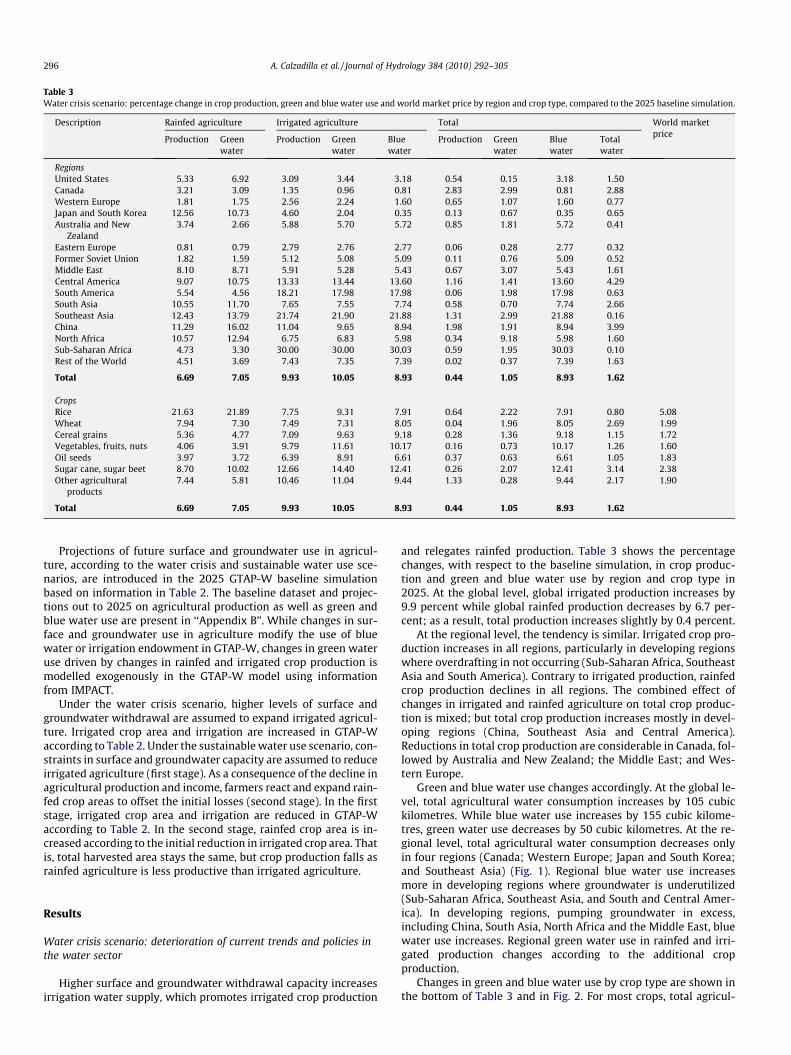
Table 3Water crisis scenario: percentage change in crop production, green and blue water use and world market price by region and crop type, compared to the 2025 baseline simulation.

Description Rainfed agriculture Irrigated agriculture Total World marketprice

Production Greenwater


Bluewater


Bluewater

Totalwater

RegionsUnited States �5.33 �6.92 3.09 3.44 3.18 0.54 �0.15 3.18 1.50Canada �3.21 �3.09 1.35 0.96 0.81 �2.83 �2.99 0.81 �2.88Western Europe �1.81 �1.75 2.56 2.24 1.60 �0.65 �1.07 1.60 �0.77Japan and South Korea �12.56 �10.73 4.60 2.04 �0.35 0.13 �0.67 �0.35 �0.65Australia and New

Zealand�3.74 �2.66 5.88 5.70 5.72 �0.85 �1.81 5.72 0.41

Eastern Europe �0.81 �0.79 2.79 2.76 2.77 �0.06 �0.28 2.77 0.32Former Soviet Union �1.82 �1.59 5.12 5.08 5.09 �0.11 �0.76 5.09 0.52Middle East �8.10 �8.71 5.91 5.28 5.43 �0.67 �3.07 5.43 1.61Central America �9.07 �10.75 13.33 13.44 13.60 1.16 �1.41 13.60 4.29South America �5.54 �4.56 18.21 17.98 17.98 �0.06 �1.98 17.98 0.63South Asia �10.55 �11.70 7.65 7.55 7.74 0.58 �0.70 7.74 2.66Southeast Asia �12.43 �13.79 21.74 21.90 21.88 1.31 �2.99 21.88 �0.16China �11.29 �16.02 11.04 9.65 8.94 1.98 1.91 8.94 3.99North Africa �10.57 �12.94 6.75 6.83 5.98 �0.34 �9.18 5.98 1.60Sub-Saharan Africa �4.73 �3.30 30.00 30.00 30.03 �0.59 �1.95 30.03 0.10Rest of the World �4.51 �3.69 7.43 7.35 7.39 �0.02 �0.37 7.39 1.63

Total �6.69 �7.05 9.93 10.05 8.93 0.44 �1.05 8.93 1.62

CropsRice �21.63 �21.89 7.75 9.31 7.91 0.64 �2.22 7.91 0.80 �5.08Wheat �7.94 �7.30 7.49 7.31 8.05 0.04 �1.96 8.05 2.69 �1.99Cereal grains �5.36 �4.77 7.09 9.63 9.18 0.28 �1.36 9.18 1.15 �1.72Vegetables, fruits, nuts �4.06 �3.91 9.79 11.61 10.17 0.16 �0.73 10.17 1.26 �1.60Oil seeds �3.97 �3.72 6.39 8.91 6.61 0.37 �0.63 6.61 1.05 �1.83Sugar cane, sugar beet �8.70 �10.02 12.66 14.40 12.41 0.26 �2.07 12.41 3.14 �2.38Other agricultural

products�7.44 �5.81 10.46 11.04 9.44 1.33 0.28 9.44 2.17 �1.90

Total �6.69 �7.05 9.93 10.05 8.93 0.44 �1.05 8.93 1.62


Projections of future surface and groundwater use in agricul-ture, according to the water crisis and sustainable water use sce-narios, are introduced in the 2025 GTAP-W baseline simulationbased on information in Table 2. The baseline dataset and projec-tions out to 2025 on agricultural production as well as green andblue water use are present in ‘‘Appendix B”. While changes in sur-face and groundwater use in agriculture modify the use of bluewater or irrigation endowment in GTAP-W, changes in green wateruse driven by changes in rainfed and irrigated crop production ismodelled exogenously in the GTAP-W model using informationfrom IMPACT.

Under the water crisis scenario, higher levels of surface andgroundwater withdrawal are assumed to expand irrigated agricul-ture. Irrigated crop area and irrigation are increased in GTAP-Waccording to Table 2. Under the sustainable water use scenario, con-straints in surface and groundwater capacity are assumed to reduceirrigated agriculture (first stage). As a consequence of the decline inagricultural production and income, farmers react and expand rain-fed crop areas to offset the initial losses (second stage). In the firststage, irrigated crop area and irrigation are reduced in GTAP-Waccording to Table 2. In the second stage, rainfed crop area is in-creased according to the initial reduction in irrigated crop area. Thatis, total harvested area stays the same, but crop production falls asrainfed agriculture is less productive than irrigated agriculture.

Results

Water crisis scenario: deterioration of current trends and policies inthe water sector

Higher surface and groundwater withdrawal capacity increasesirrigation water supply, which promotes irrigated crop production

and relegates rainfed production. Table 3 shows the percentagechanges, with respect to the baseline simulation, in crop produc-tion and green and blue water use by region and crop type in2025. At the global level, global irrigated production increases by9.9 percent while global rainfed production decreases by 6.7 per-cent; as a result, total production increases slightly by 0.4 percent.

At the regional level, the tendency is similar. Irrigated crop pro-duction increases in all regions, particularly in developing regionswhere overdrafting in not occurring (Sub-Saharan Africa, SoutheastAsia and South America). Contrary to irrigated production, rainfedcrop production declines in all regions. The combined effect ofchanges in irrigated and rainfed agriculture on total crop produc-tion is mixed; but total crop production increases mostly in devel-oping regions (China, Southeast Asia and Central America).Reductions in total crop production are considerable in Canada, fol-lowed by Australia and New Zealand; the Middle East; and Wes-tern Europe.

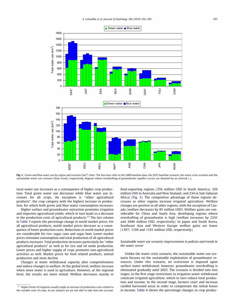
Green and blue water use changes accordingly. At the global le-vel, total agricultural water consumption increases by 105 cubickilometres. While blue water use increases by 155 cubic kilome-tres, green water use decreases by 50 cubic kilometres. At the re-gional level, total agricultural water consumption decreases onlyin four regions (Canada; Western Europe; Japan and South Korea;and Southeast Asia) (Fig. 1). Regional blue water use increasesmore in developing regions where groundwater is underutilized(Sub-Saharan Africa, Southeast Asia, and South and Central Amer-ica). In developing regions, pumping groundwater in excess,including China, South Asia, North Africa and the Middle East, bluewater use increases. Regional green water use in rainfed and irri-gated production changes according to the additional cropproduction.

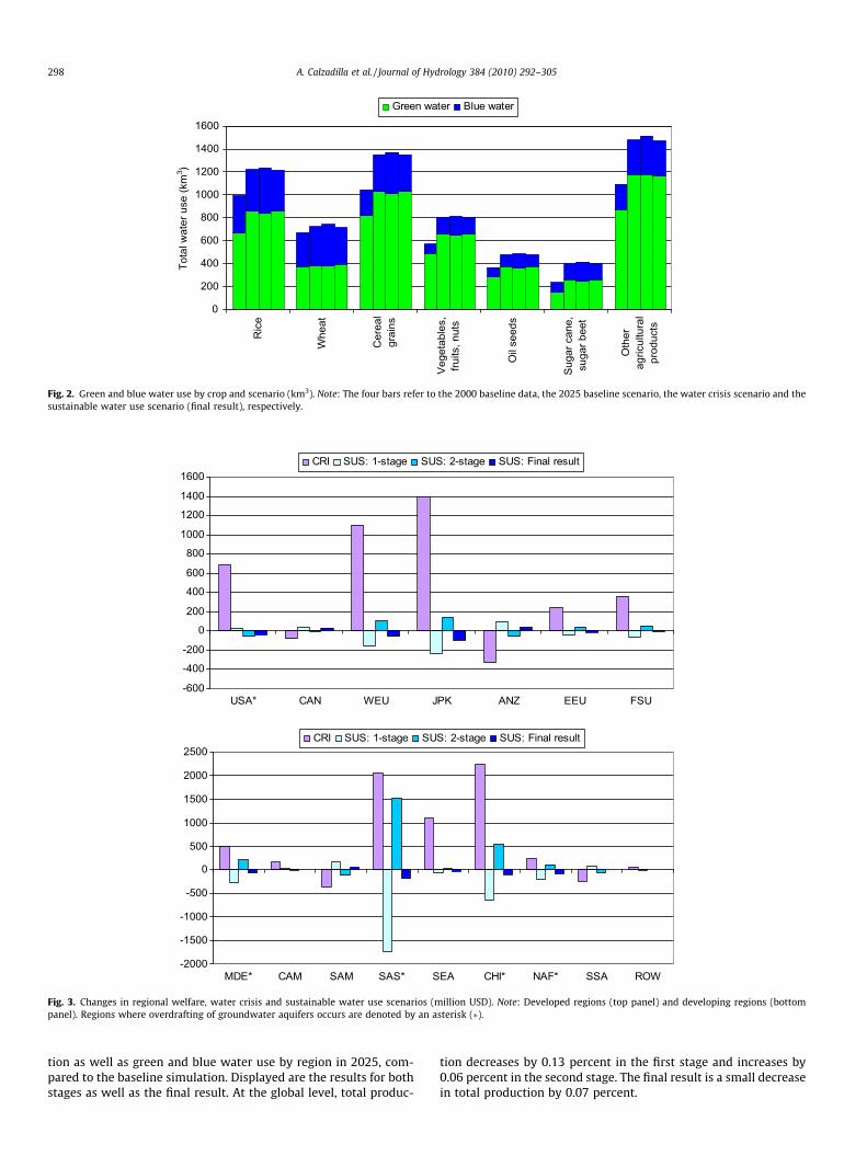
Changes in green and blue water use by crop type are shown inthe bottom of Table 3 and in Fig. 2. For most crops, total agricul-

0

200

400

600

800

1000

1200

1400

1600

1800

SA

S*

CH

I*

SSA

SEA

SA

M

US

A*

FSU

CA

M

Tota

l wat

er u

se (k

m 3 )

Green water Blue water

0

20

40

60

80

100

120

140

160

180

MD

E*

EE

U

WE

U

NA

F*

AN

Z

CA

N

JPK

RO

W

Tota

l wat

er u

se (k

m 3 )


Fig. 1. Green and blue water use by region and scenario (km3). Note: The four bars refer to the 2000 baseline data, the 2025 baseline scenario, the water crisis scenario and thesustainable water use scenario (final result), respectively. Regions where overdrafting of groundwater aquifers occurs are denoted by an asterisk (�).


tural water use increases as a consequence of higher crop produc-tion. Total green water use decreases while blue water use in-creases for all crops. An exception is ‘‘other agriculturalproducts”, the crop category with the highest increase in produc-tion, for which both green and blue water consumption increases.

Higher surface and groundwater extraction promotes irrigationand improves agricultural yields, which in turn leads to a decreasein the production costs of agricultural products.12 The last columnin Table 3 reports the percentage change in world market prices. Forall agricultural products, world market prices decrease as a conse-quence of lower production costs. Reductions in world market pricesare considerable for rice, sugar cane and sugar beet. Lower marketprices stimulate consumption and total production of all agriculturalproducts increases. Total production increases particularly for ‘‘otheragricultural products” as well as for rice and oil seeds production.Lower prices and higher supply of crops promotes non-agriculturalactivities as well. Market prices for food related products, animalproduction and meat decline.

Changes in water withdrawal capacity alter competitivenessand induce changes in welfare. At the global level, welfare increasewhen more water is used in agriculture. However, at the regionallevel, the results are more mixed. Welfare decreases mainly in

12 Higher levels of irrigation usually imply an increase of production costs related tothe variable costs of crops. In our analysis we are not able to take that into account
.
food-exporting regions (356 million USD in South America; 326million USD in Australia and New Zealand; and 234 in Sub-SaharanAfrica) (Fig. 3). The competitive advantage of those regions de-creases as other regions increase irrigated agriculture. Welfarechanges are positive in all other regions, with the exception of Can-ada (welfare decreases by 85 million USD). Welfare gains are con-siderable for China and South Asia, developing regions whereoverdrafting of groundwater is high (welfare increases by 2241and 2044 million USD, respectively). In Japan and South Korea,Southeast Asia and Western Europe welfare gains are lower(1397; 1104 and 1101 million USD, respectively).

Sustainable water use scenario: improvements in policies and trends inthe water sector

Unlike the water crisis scenario, the sustainable water use sce-nario focuses on the sustainable exploitation of groundwater re-sources. Under this scenario, no restriction is imposed uponsurface water withdrawal; however, groundwater overdrafting iseliminated gradually until 2025. The scenario is divided into twostages, in the first stage restrictions in irrigation water withdrawalconstrain irrigated agriculture, which in turn reduce total produc-tion and income. In the second stage, farmers react and increaserainfed harvested areas in order to compensate the initial lossesin income. Table 4 shows the percentage changes in crop produc-

0

200

400

600

800

1000

1200

1400

1600

Ric

e

Whe

at

Cer

eal

grai

ns

Vege

tabl

es,

fruits

, nut

s

Oil

seed

s

Suga

r can

e,su

gar b

eet

Oth

erag

ricul

tura

lpr

oduc

ts

Tota

l wat

er u

se (k

m 3 )


Fig. 2. Green and blue water use by crop and scenario (km3). Note: The four bars refer to the 2000 baseline data, the 2025 baseline scenario, the water crisis scenario and thesustainable water use scenario (final result), respectively.

-600

-400

-200

0

200

400

600

800

1000

1200

1400

1600

USA* CAN WEU JPK ANZ EEU FSU

CRI SUS: 1-stage SUS: 2-stage SUS: Final result

-2000

-1500

-1000

-500

0

500

1000

1500

2000

2500

MDE* CAM SAM SAS* SEA CHI* NAF* SSA ROW

CRI SUS: 1-stage SUS: 2-stage SUS: Final result

Fig. 3. Changes in regional welfare, water crisis and sustainable water use scenarios (million USD). Note: Developed regions (top panel) and developing regions (bottompanel). Regions where overdrafting of groundwater aquifers occurs are denoted by an asterisk (�).


tion as well as green and blue water use by region in 2025, com-pared to the baseline simulation. Displayed are the results for bothstages as well as the final result. At the global level, total produc-

tion decreases by 0.13 percent in the first stage and increases by0.06 percent in the second stage. The final result is a small decreasein total production by 0.07 percent.

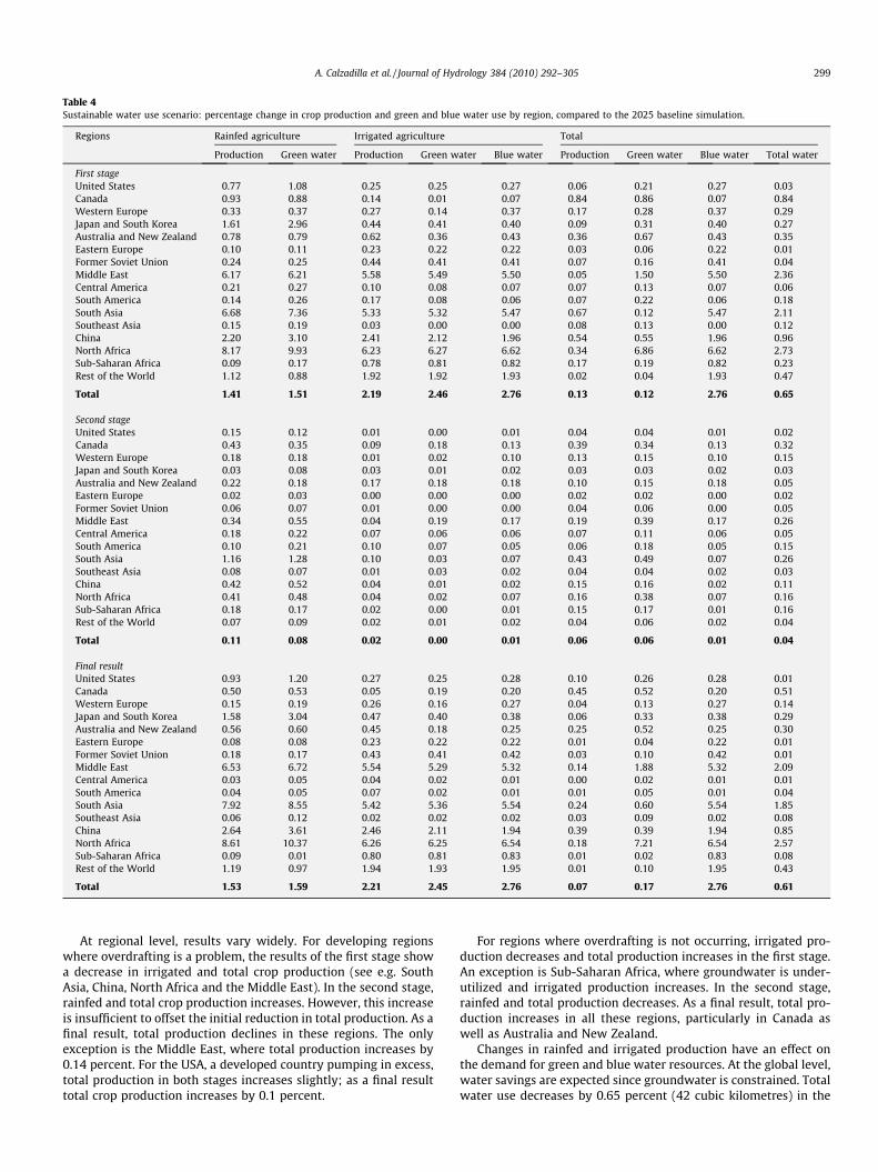
Table 4Sustainable water use scenario: percentage change in crop production and green and blue water use by region, compared to the 2025 baseline simulation.

Regions Rainfed agriculture Irrigated agriculture Total

Production Green water Production Green water Blue water Production Green water Blue water Total water

First stageUnited States 0.77 1.08 �0.25 �0.25 �0.27 0.06 0.21 �0.27 �0.03Canada 0.93 0.88 �0.14 0.01 0.07 0.84 0.86 0.07 0.84Western Europe 0.33 0.37 �0.27 �0.14 0.37 0.17 0.28 0.37 0.29Japan and South Korea 1.61 2.96 �0.44 �0.41 �0.40 0.09 0.31 �0.40 0.27Australia and New Zealand 0.78 0.79 �0.62 �0.36 �0.43 0.36 0.67 �0.43 0.35Eastern Europe 0.10 0.11 �0.23 �0.22 �0.22 0.03 0.06 �0.22 0.01Former Soviet Union 0.24 0.25 �0.44 �0.41 �0.41 0.07 0.16 �0.41 0.04Middle East 6.17 6.21 �5.58 �5.49 �5.50 �0.05 1.50 �5.50 �2.36Central America 0.21 0.27 �0.10 �0.08 �0.07 0.07 0.13 �0.07 0.06South America 0.14 0.26 �0.17 �0.08 �0.06 0.07 0.22 �0.06 0.18South Asia 6.68 7.36 �5.33 �5.32 �5.47 �0.67 0.12 �5.47 �2.11Southeast Asia 0.15 0.19 �0.03 0.00 0.00 0.08 0.13 0.00 0.12China 2.20 3.10 �2.41 �2.12 �1.96 �0.54 �0.55 �1.96 �0.96North Africa 8.17 9.93 �6.23 �6.27 �6.62 �0.34 6.86 �6.62 �2.73Sub-Saharan Africa 0.09 0.17 0.78 0.81 0.82 0.17 0.19 0.82 0.23Rest of the World 1.12 0.88 �1.92 �1.92 �1.93 �0.02 0.04 �1.93 �0.47

Total 1.41 1.51 �2.19 �2.46 �2.76 �0.13 0.12 �2.76 �0.65

Second stageUnited States 0.15 0.12 �0.01 0.00 �0.01 0.04 0.04 �0.01 0.02Canada �0.43 �0.35 0.09 0.18 0.13 �0.39 �0.34 0.13 �0.32Western Europe �0.18 �0.18 0.01 �0.02 �0.10 �0.13 �0.15 �0.10 �0.15Japan and South Korea �0.03 0.08 �0.03 0.01 0.02 �0.03 0.03 0.02 0.03Australia and New Zealand �0.22 �0.18 0.17 0.18 0.18 �0.10 �0.15 0.18 �0.05Eastern Europe �0.02 �0.03 0.00 0.00 0.00 �0.02 �0.02 0.00 �0.02Former Soviet Union �0.06 �0.07 0.01 0.00 0.00 �0.04 �0.06 0.00 �0.05Middle East 0.34 0.55 0.04 0.19 0.17 0.19 0.39 0.17 0.26Central America �0.18 �0.22 0.07 0.06 0.06 �0.07 �0.11 0.06 �0.05South America �0.10 �0.21 0.10 0.07 0.05 �0.06 �0.18 0.05 �0.15South Asia 1.16 1.28 �0.10 �0.03 �0.07 0.43 0.49 �0.07 0.26Southeast Asia �0.08 �0.07 0.01 0.03 0.02 �0.04 �0.04 0.02 �0.03China 0.42 0.52 �0.04 0.01 0.02 0.15 0.16 0.02 0.11North Africa 0.41 0.48 �0.04 0.02 0.07 0.16 0.38 0.07 0.16Sub-Saharan Africa �0.18 �0.17 0.02 0.00 0.01 �0.15 �0.17 0.01 �0.16Rest of the World 0.07 0.09 �0.02 �0.01 �0.02 0.04 0.06 �0.02 0.04

Total 0.11 0.08 �0.02 0.00 �0.01 0.06 0.06 �0.01 0.04

Final resultUnited States 0.93 1.20 �0.27 �0.25 �0.28 0.10 0.26 �0.28 �0.01Canada 0.50 0.53 �0.05 0.19 0.20 0.45 0.52 0.20 0.51Western Europe 0.15 0.19 �0.26 �0.16 0.27 0.04 0.13 0.27 0.14Japan and South Korea 1.58 3.04 �0.47 �0.40 �0.38 0.06 0.33 �0.38 0.29Australia and New Zealand 0.56 0.60 �0.45 �0.18 �0.25 0.25 0.52 �0.25 0.30Eastern Europe 0.08 0.08 �0.23 �0.22 �0.22 0.01 0.04 �0.22 �0.01Former Soviet Union 0.18 0.17 �0.43 �0.41 �0.42 0.03 0.10 �0.42 �0.01Middle East 6.53 6.72 �5.54 �5.29 �5.32 0.14 1.88 �5.32 �2.09Central America 0.03 0.05 �0.04 �0.02 �0.01 0.00 0.02 �0.01 0.01South America 0.04 0.05 �0.07 �0.02 �0.01 0.01 0.05 �0.01 0.04South Asia 7.92 8.55 �5.42 �5.36 �5.54 �0.24 0.60 �5.54 �1.85Southeast Asia 0.06 0.12 �0.02 0.02 0.02 0.03 0.09 0.02 0.08China 2.64 3.61 �2.46 �2.11 �1.94 �0.39 �0.39 �1.94 �0.85North Africa 8.61 10.37 �6.26 �6.25 �6.54 �0.18 7.21 �6.54 �2.57Sub-Saharan Africa �0.09 �0.01 0.80 0.81 0.83 0.01 0.02 0.83 0.08Rest of the World 1.19 0.97 �1.94 �1.93 �1.95 0.01 0.10 �1.95 �0.43

Total 1.53 1.59 �2.21 �2.45 �2.76 �0.07 0.17 �2.76 �0.61


At regional level, results vary widely. For developing regionswhere overdrafting is a problem, the results of the first stage showa decrease in irrigated and total crop production (see e.g. SouthAsia, China, North Africa and the Middle East). In the second stage,rainfed and total crop production increases. However, this increaseis insufficient to offset the initial reduction in total production. As afinal result, total production declines in these regions. The onlyexception is the Middle East, where total production increases by0.14 percent. For the USA, a developed country pumping in excess,total production in both stages increases slightly; as a final resulttotal crop production increases by 0.1 percent.

For regions where overdrafting is not occurring, irrigated pro-duction decreases and total production increases in the first stage.An exception is Sub-Saharan Africa, where groundwater is under-utilized and irrigated production increases. In the second stage,rainfed and total production decreases. As a final result, total pro-duction increases in all these regions, particularly in Canada aswell as Australia and New Zealand.

Changes in rainfed and irrigated production have an effect onthe demand for green and blue water resources. At the global level,water savings are expected since groundwater is constrained. Totalwater use decreases by 0.65 percent (42 cubic kilometres) in the


first stage and increases slightly by 0.04 percent (3 cubic kilome-tres) in the second stage. The final result is a decrease in total wateruse by 0.61 percent (40 cubic kilometres). While blue water usedecreases, total green water use increases in both stages.

At the regional level, green and blue water use varies widely.For regions where overdrafting is a problem, blue and total wateruse decrease in the first stage, particularly in North Africa, the Mid-dle East and South Asia. In the second stage blue as well as totalwater use increases (exceptions are the USA and South Asia). How-ever, the final result, taken the results of stages 1 and 2 together,blue and total water use decrease (Table 4 and Fig. 1). Together to-tal water savings in all these regions reach 42 cubic kilometres.South Asia accounts for more than two-thirds of the total watersavings in these regions. For regions where overdrafting is notoccurring, results are less pronounced.

Changes in green and blue water use by crop type are reportedin Table 5. In the first stage, when groundwater withdrawal is lim-ited, there is a shift in production from irrigated to rainfed agricul-ture. Global irrigated production decreases, which implies areduction in green and blue water use. By contrast, global rainfedproduction and green water use increases. Rainfed production in-creases considerably for rice and wheat (5.1 and 3.2 percent,respectively). As a result, global production decreases by 0.1 per-cent and water savings reach 42 cubic kilometres.

In the second stage, when rainfed areas expand to neutralizeproduction and income losses, global rainfed and total productionincreases slightly. Taking the results of both stages together, the fi-nal results show, at the bottom of Table 5, a decrease in total pro-duction for all crops. The sectors ‘‘Other agricultural products” andrice have the largest decrease in total production. While blue water

Table 5Sustainable water use scenario: percentage change in crop production, green and blue wate

Crops Rainfed agriculture Irrigated agriculture



Bluwa

First stageRice 5.11 4.49 �1.95 �2.35 �2Wheat 3.19 2.91 �3.15 �2.56 �4Cereal grains 0.94 0.84 �1.22 �1.51 �1Vegetables, fruits, nuts 0.99 0.75 �2.47 �2.30 �2Oil seeds 0.69 0.71 �1.04 �1.63 �1Sugar cane, sugar beet 1.24 0.81 �1.93 �1.43 �2Other agricultural

products1.88 1.48 �2.67 �3.52 �3

Total 1.41 1.51 �2.19 �2.46 �2

Second stageRice 0.43 0.27 0.02 0.00 0Wheat 0.05 0.01 0.04 0.06 0Cereal grains 0.05 0.05 0.00 �0.03 �0Vegetables, fruits, nuts 0.14 0.10 �0.09 �0.13 �0Oil seeds �0.01 �0.03 0.05 0.05 �0Sugar cane, sugar beet 0.09 0.04 �0.01 0.01 �0Other agricultural

products0.15 0.10 �0.02 0.04 0

Total 0.11 0.08 �0.02 0.010. �0

Final resultRice 5.56 4.78 �1.93 �2.36 �2Wheat 3.24 2.92 �3.11 �2.51 �4Cereal grains 0.99 0.89 �1.22 �1.54 �1Vegetables, fruits, nuts 1.12 0.85 �2.55 �2.43 �3Oil seeds 0.68 0.68 �0.99 �1.58 �1Sugar cane, sugar beet 1.33 0.84 �1.93 �1.42 �2Other agricultural

products2.03 1.58 �2.70 �3.49 �2

Total 1.53 1.59 �2.21 �2.45 �2

use declines for all crops, total green water use increases for allcrops except for ‘‘other agricultural products” (Fig. 2). The finalwater savings reach 40 cubic kilometres. Water savings are markedfor the crops ‘‘other agricultural products”, wheat and rice.

The last column in Table 5 shows the changes in world marketprices for all crop types. When groundwater use is constrained(first stage), world market prices increase for all crops and for agri-cultural related products (food products, animal production andmeat production). World market prices increase mainly for rice;sugar cane and sugar beet; and wheat. In the second stage, worldmarket prices decrease for all crops when rainfed areas are in-creased. World market prices decline mainly for oil seeds and veg-etables, fruits and nuts. The combined effect of both stages shows adecrease in price for oil seeds and vegetables, fruits and nuts. Forall other crops including agricultural related activities, world mar-ket prices increase.

Reducing groundwater overdraft world-wide alters the compet-itiveness of regions and induces changes in welfare. At the globallevel, welfare declines in the first stage by 2993 million USD andincreases by 2490 million USD in the second stage. Taken both re-sults together, welfare declines by 503 million USD (Fig. 3). At theregional level, welfare effects are diverse depending on the region.In the first stage, welfare decreases for most of the regions, butmainly for developing regions where overdrafting is excessive. InSouth Asia, China and the Middle East welfare decreases by1721; 643 and 274 million USD, respectively. In this stage, welfaregains are observable mainly in developing regions where ground-water use is underutilized. Welfare increases in South America,Sub-Saharan Africa and Central America by 167, 77 and 20 millionUSD, respectively. In the second stage, welfare changes for all re-

r use and world market price by crop type, compared to the 2025 baseline simulation.

Total World marketprice

eter


Bluewater

Totalwater

.85 �0.24 0.18 �2.85 �0.72 1.50

.30 �0.09 0.91 �4.30 �1.51 0.84

.38 �0.04 0.28 �1.38 �0.11 0.41

.91 �0.07 0.13 �2.91 �0.43 0.49

.24 �0.04 0.13 �1.24 �0.18 0.64

.52 �0.09 0.08 �2.52 �0.86 0.98

.00 �0.35 �0.33 �3.00 �0.88 0.65

.76 �0.13 0.12 �2.76 �0.65

.00 0.13 0.10 0.00 0.07 �0.25

.05 0.04 0.02 0.05 0.03 �0.24

.02 0.02 0.03 �0.02 0.02 �0.28

.10 0.07 0.05 �0.10 0.02 �0.76

.01 0.02 �0.01 �0.01 �0.01 �0.86

.05 0.05 0.03 �0.05 0.00 �0.46

.01 0.07 0.08 0.01 0.06 �0.49

.01 0.06 0.06 �0.01 0.04

.85 �0.12 0.28 �2.85 �0.65 1.25

.25 �0.05 0.94 �4.25 �1.48 0.60

.39 �0.02 0.31 �1.39 �0.09 0.12

.00 0.00 0.18 �3.00 �0.40 �0.27

.25 �0.02 0.13 �1.25 �0.19 �0.22

.56 �0.04 0.11 �2.56 �0.85 0.52

.99 �0.28 �0.25 �2.99 �0.82 0.15

.76 �0.07 0.17 �2.76 �0.61


gions have an opposite sign than in the first stage. In South Asia,China and the Middle East welfare increases by 1537; 546 and221 million USD, respectively. In South America, Sub-Saharan Afri-ca and Central America welfare declines by 115, 61 and 12 millionUSD, respectively.

Regional welfare gains in the second stage are considerablylower or more than offset welfare losses in the first stage. Takenthe results of stages 1 and 2 together, final welfare changes arenegative for regions with excessive overdraft. Welfare losses arehighest for South Asia and China (183 and 96 million USD, respec-tively). For regions where groundwater use is underutilized, wel-fare changes are mostly positive. Welfare increases in SouthAmerica, Sub-Saharan Africa and Central America by 52, 16 and 8million USD, respectively. The only exception is Southeast Asia,where welfare decreases by 23 million USD. For the rest of the re-gions where groundwater overdraft is not problematic, welfarechanges are mostly negative. The highest decreases in welfareare present in Japan and South Korea; and Western Europe (97and 59 million USD, respectively). Exceptions are Australia andNew Zealand; and Canada, where welfare increases by 40 and 25million USD, respectively.

Discussion and conclusions

In our analysis, the water crisis and sustainable water use sce-narios lead to different patterns in agricultural water consumption.While the water crisis scenario explores a deterioration in currentconditions and policies in the water sector, the sustainable wateruse scenario assumes an improvement and eliminates groundwa-ter overdraft world-wide.

Irrigation water use is promoted under the water crisis scenario.At the global level, total production increases by 1.6 percent. Irri-gated production expands suppressing rainfed production. As a re-sult, total agricultural water consumption increases; irrigationwater use increases even more, while the use of rain water falls.Higher levels of irrigation increase agricultural yields and allowfarmers to obtain more output per unit of input, which in turn re-duces production costs and crop prices. World market prices de-crease for all crops and for agricultural related products (foodproducts, animal production and meat production). Global welfarewould increase by 9 billion USD.

An opposite picture is obtained under the sustainable use sce-nario. At the global level, total elimination of groundwater over-draft decreases total production moderately. As groundwater useis limited, irrigated production decreases and rainfed productionincreases. Total water consumption decreases. World marketprices increase, but not for all crops. Global welfare falls by 0.5 bil-lion USD.

At the regional level, results vary widely. Under the water crisisscenario, total production increases mainly in China, SoutheastAsia and Central America and decreases principally in Canadaand Australia and New Zealand. Under the sustainable water usescenario, total production decreases only in China, South Asiaand North Africa and increases in all other regions mainly in Can-ada and Australia and New Zealand.

Under the water crisis scenario, irrigated production increasesin all regions but more in developing regions where overdraft isnot a problem. Irrigated production increases less in regions withoverdraft. Under the sustainable water use scenario, irrigated pro-duction decreases in all regions, but mainly in developing regionswith overdraft. Irrigated production increases only in Sub-SaharanAfrica, where groundwater is underutilized.

Under the water crisis scenario, irrigated and total productionincreases for all crops, while rainfed production decreases. Theopposite occurs under the sustainable water use scenario.

Regional use of green and blue water resources changes accord-ing to the additional rainfed and irrigated crop production. In abso-lute terms, under the water crisis scenario, most of the total waterconsumption occurs in regions where overdrafting is a problem,mainly in China, South East Asia and the USA. For most regions, to-tal green water use decreases and blue water use increases. In Ja-pan and South Korea, both green and blue water consumptiondecreases slightly. In China, both green and blue water consump-tion increases. Under the sustainable water use scenario, waterrestrictions affect predominantly regions where groundwater re-sources are on pressure. Total water consumption decrease mainlyin South Asia, China and the Middle East.

In both scenarios, welfare changes go beyond changes in agri-cultural water consumption. Welfare changes in regions wherewater use changes, but it spills over to other regions too. Underthe sustainable water use scenario, global and regional welfarelosses could be significant if farmers do not increase rainfed areasto offset initial losses in production and income due to irrigationconstraints.

The results reveal a clear trade-off between agricultural produc-tion, and hence human welfare as measurable by consumption ofmarket goods on the one hand and nature conservation on theother hand. There is more water available for agriculture in thewater crisis scenario than in business as usual scenario, and wel-fare is higher. The sustainable water use scenario has less waterfor agriculture, and lower welfare. However, the amount of wateravailable to the natural environment moves in the opposite direc-tion: More water for agriculture means less water for nature. Thispaper does not quantify the benefits of water to nature. It does,however, quantify the welfare implications of restricting orincreasing the human take of total water. In the water crisis sce-nario, for instance, the human benefits of taking 105 cubic kilome-tres of water out of nature are some 9 billion USD – less than $1.3per person. The welfare costs of the policies presumed in the sus-tainable water use scenario are also very small.

Several limitations apply to the above results. First, our analysisis based on regional averages. We do not differentiate between dif-ferent regions within a country. China is an example of such acountry. Although on average water is not short, water supply isa problem in Northern China, where groundwater overexploitationoccurs. In our sustainable water use scenario we try to account forthis effect. Second, under the water crisis scenario, expansion ofirrigated areas is driven by the availability of water for irrigation,we do not account for possible environmental effects of land usechanges. Third, under the water crisis scenario, we do not considerany cost or investment associated with irrigation expansion.Therefore, our results might overestimate the benefits of this sce-nario. Forth, we implicitly assume, for the sustainable water crisisscenario, availability and accessibility of green water resourceswhen rainfed agriculture expands. In addition, some areas mightbe more suitable for rainfed agriculture than others. As a conse-quence, the initial loss in income might not be compensated asmuch as indicated in our scenario. Fifth, the GTAP-W model con-siders water quantity and prices but ignores non-market benefitsor costs of water use. For instance, the model is unable to predictthe direct ecological impact of limiting groundwater use. Sixth,our analysis does not account for surface and groundwater useapart from agriculture, since the necessary data are missing. Theseissues should be addressed in future research.

Acknowledgements

We had useful discussions about the topics of this article withHolger Hoff and participants at the Global Green–Blue Initiativeworkshop in Stockholm. This article is supported by the FederalMinistry for Economic Cooperation and Development, Germany


under the project ‘‘Food and Water Security under Global Change:Developing Adaptive Capacity with a Focus on Rural Africa,” whichforms part of the CGIAR Challenge Program on Water and Food,and by the Michael Otto Foundation for Environmental Protection.

Appendix A

See Table A1 and Fig. A1.

Table A1Aggregations in GTAP-W.

A. Regional aggregation B. Sectoral aggregation1. USA – United States 1. Rice – rice2. CAN – Canada 2. Wheat – wheat3. WEU – Western Europe 3. CerCrops – cereal grains (maize, millet,4. JPK – Japan and South Korea sorghum and other grains)5. ANZ – Australia and New

Zealand4. VegFruits – vegetable, fruits, nuts

6. EEU – Eastern Europe 5. OilSeeds – oil seeds7. FSU – Former Soviet Union 6. Sug_Can – sugar cane, sugar beet8. MDE – Middle East 7. Oth_Agr – other agricultural products9. CAM – Central America 8. Animals – animals10. SAM – South America 9. Meat – meat11. SAS – South Asia 10. Food_Prod – food products12. SEA – Southeast Asia 11. Forestry – forestry13. CHI – China 12. Fishing – fishing14. NAF – North Africa 13. Coal – coal15. SSA – Sub-Saharan Africa 14. Oil – oil16. ROW – Rest of the World 15. Gas – gas

16. Oil_Pcts – oil productsC. Endowments 17. Electricity – electricityWtr – irrigation 18. Water – waterLnd – irrigated land 19. En_Int_Ind – energy intensive

industriesRfLand – rainfed land 20. Oth_Ind – other industry and servicesPsLand – pasture land 21. Mserv – market servicesLab – labour 22. NMServ – non-market servicesCapital – capitalNatlRes – natural resources

Irrigated Land-Water Rainfed Pasture Natural Labo Composite Land Land Resources

Irrigated Irrigation Land

σσσσLW

σVAE

Value-added (Including energy inputs)

Fig. A1. Nested tree structure for industrial production process in GTAP-W (truncated).irrigated land and irrigation (bold letters). r is the elasticity of substitution between vaprimary factors, rLW is the elasticity of substitution between irrigated land and irrigatiois the elasticity of substitution between domestic and imported inputs and rM is the el

Appendix B. Future baseline simulation

To obtain a 2025 benchmark equilibrium dataset for the GTAP-W model we use the methodology described by Dixon and Rimmer(2002). This methodology allows us to find a hypothetical generalequilibrium state in the future imposing forecasted values for somekey economic variables in the initial calibration dataset. In thisway, we impose forecasted changes in regional endowments (la-bour, capital, natural resources, rainfed land, irrigated land andirrigation), in regional factor-specific and multi-factor productivityand in regional population. We use estimates of the regional labourproductivity, labour stock and capital stock from the G-Cubedmodel, a multicountry, multisector intertemporal general equilib-rium model of the world economy developed by McKibbin andWilcoxen (1998). Changes in the allocation of rainfed and irrigatedland within a region as well as irrigation and agricultural land pro-ductivity are implemented according to the values obtained by theIMPACT model. The information supplied by the IMPACT model(demand and supply of water, demand and supply of food, rainfedand irrigated production and rainfed and irrigated area) providesthe GTAP-W model with detailed information for a robust calibra-tion of a new dataset. Finally, we use the medium variant popula-tion estimates for 2025 from the Population Division of the UnitedNations (United Nations, 2004).

Compared to the 2000 baseline data (Table B1), the IMPACTmodel projects a growth in both harvested crop area as well as cropproductivity for 2025 under normal climate conditions (Table B2).The world’s crop harvested area is expected to increases by about1.4 percent between 2000 and 2025. This is equivalent to a totalarea of 1.3 billion hectares in 2025, 34.4 percent of which is underirrigation. For the same period, green water used (effective rainfall)in rainfed areas is expected to increase by 27.2 percent; and bothgreen and blue water used (water diverted from water systems)in irrigated areas are expected to increase by 33.7 and 32.1 percent,respectively. As a result, total water used in agriculture is expectedto rise by 30.4 percent, to 6466 cubic kilometres in 2025.

Farmers in Sub-Saharan Africa and South Asia use around 37percent of the world’s rainfed area in 2025, which accounts for

Capital Energy Composite

σKE

r Capital-Energy Composite

Region 1 … Region r

σM

Domestic Foreign

σD

σ = 0

All other inputs (Excluding energy inputs but including energy feedstock)

Output

Note: The original land endowment has been split into pasture land, rainfed land,lue-added and intermediate inputs, rVAE is the elasticity of substitution between

n, rKE is the elasticity of substitution between capital and the energy composite, rDasticity of substitution between imported inputs.

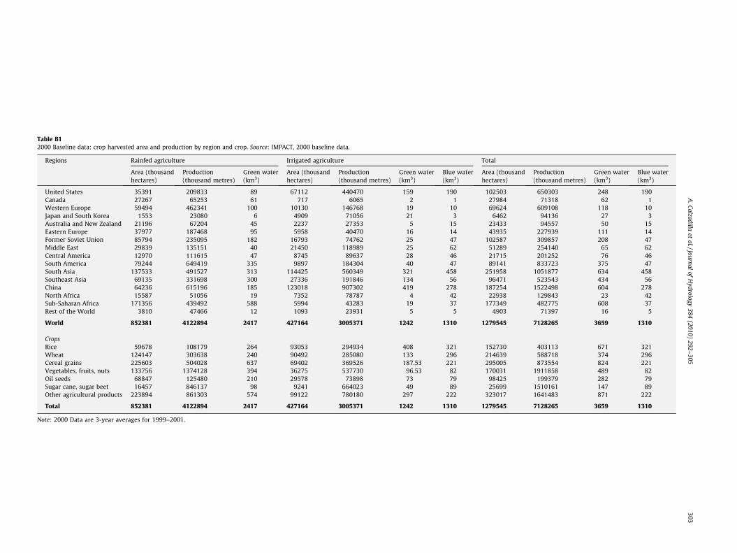
Table B12000 Baseline data: crop harvested area and production by region and crop. Source: IMPACT, 2000 baseline data.


Area (thousandhectares)

Production(thousand metres)

Green water(km3)



Green water(km3)

Blue water(km3)



Green water(km3)

Blue water(km3)

United States 35391 209833 89 67112 440470 159 190 102503 650303 248 190Canada 27267 65253 61 717 6065 2 1 27984 71318 62 1Western Europe 59494 462341 100 10130 146768 19 10 69624 609108 118 10Japan and South Korea 1553 23080 6 4909 71056 21 3 6462 94136 27 3Australia and New Zealand 21196 67204 45 2237 27353 5 15 23433 94557 50 15Eastern Europe 37977 187468 95 5958 40470 16 14 43935 227939 111 14Former Soviet Union 85794 235095 182 16793 74762 25 47 102587 309857 208 47Middle East 29839 135151 40 21450 118989 25 62 51289 254140 65 62Central America 12970 111615 47 8745 89637 28 46 21715 201252 76 46South America 79244 649419 335 9897 184304 40 47 89141 833723 375 47South Asia 137533 491527 313 114425 560349 321 458 251958 1051877 634 458Southeast Asia 69135 331698 300 27336 191846 134 56 96471 523543 434 56China 64236 615196 185 123018 907302 419 278 187254 1522498 604 278North Africa 15587 51056 19 7352 78787 4 42 22938 129843 23 42Sub-Saharan Africa 171356 439492 588 5994 43283 19 37 177349 482775 608 37Rest of the World 3810 47466 12 1093 23931 5 5 4903 71397 16 5

World 852381 4122894 2417 427164 3005371 1242 1310 1279545 7128265 3659 1310

CropsRice 59678 108179 264 93053 294934 408 321 152730 403113 671 321Wheat 124147 303638 240 90492 285080 133 296 214639 588718 374 296Cereal grains 225603 504028 637 69402 369526 187.53 221 295005 873554 824 221Vegetables, fruits, nuts 133756 1374128 394 36275 537730 96.53 82 170031 1911858 489 82Oil seeds 68847 125480 210 29578 73898 73 79 98425 199379 282 79Sugar cane, sugar beet 16457 846137 98 9241 664023 49 89 25699 1510161 147 89Other agricultural products 223894 861303 574 99122 780180 297 222 323017 1641483 871 222

Total 852381 4122894 2417 427164 3005371 1242 1310 1279545 7128265 3659 1310

Note: 2000 Data are 3-year averages for 1999–2001.

A.Calzadilla

etal./Journal

ofH

ydrology384

(2010)292–

305303

Table B22025 Baseline simulation: crop harvested area and production by region and crop. Source: IMPACT.




Green water(km3)



Green water(km3)

Blue water(km3)



Green water(km3)

Blue water(km3)

United States 33561 282634 95 68312 649118 178 269 101873 931752 272 269Canada 24547 84579 64 668 7816 2 2 25216 92395 65 2Western Europe 49655 471745 82 9206 170610 17 13 58861 642355 99 13Japan and South Korea 1330 25507 7 4339 72386 25 2 5669 97893 32 2Australia and New Zealand 20574 87458 45 2211 37586 5 21 22785 125044 50 21Eastern Europe 33620 214995 91 5411 56306 15 26 39031 271301 106 26Former Soviet Union 83041 327597 194 16850 107271 28 62 99890 434868 222 62Middle East 30330 171058 41 22838 192787 28 84 53169 363844 69 84Central America 13197 177760 63 9543 149400 40 63 22740 327161 103 63South America 89653 1305413 468 11725 391766 60 79 101378 1697179 528 79South Asia 117502 567087 384 129479 893522 511 594 246981 1460609 895 594Southeast Asia 73223 457800 409 27488 307826 178 76 100711 765626 587 76China 61143 710893 227 120294 1041731 526 316 181436 1752624 753 316North Africa 16117 79552 18 7820 114835 4 55 23937 194388 22 55Sub-Saharan Africa 200093 727357 873 8311 98412 37 62 208404 825769 910 62Rest of the World 4122 78566 16 1260 47376 7 8 5382 125941 23 8

Total 851709 5770002 3075 445754 4338747 1660 1730 1297463 10108749 4736 1730

CropsRice 52329 107187 318 91357 335710 542 365 143686 442897 860 365Wheat 115502 370764 245 88649 397007 141 336 204150 767771 387 336Cereal grains 221740 682485 787 74630 566363 244 322 296370 1248848 1031 322Vegetables, fruits, nuts 142260 1838783 523 41014 806515 135 147 183274 2645298 658 147Oil seeds 71325 137662 278 30735 99416 90 111 102060 237078 368 111Sugar cane, sugar beet 21827 1662782 173 11997 1202418 84 144 33823 2865200 257 144Other agricultural products 226726 970340 751 107373 931317 425 305 334099 1901657 1175 305

Total 851709 5770002 3075 445754 4338747 1660 1730 1297463 10108749 4736 1730

Note: Linear interpolation from IMPACT 2050 simulation with no climate change.

304A

.Calzadillaet

al./Journalof

Hydrology

384(2010)

292–305

Fig. B1. Irrigated harvested area as a share of total crop harvested area, 2025 baseline simulation. Source: IMPACT.


about 24 percent of the world’s crop area (Table B2). Similarly, 62percent of the world’s irrigated area in 2025 is in Asia, which ac-counts for about 21 percent of the world’s crop area. Sub-SaharanAfrica, South Asia and China use more than half of total greenwater used world-wide. Principal users of blue water are SouthAsia, China and the United States, using almost 70 percent of thetotal. On the crop level, rainfed production of ‘‘cereal grains” and‘‘other agricultural product” consumes about half of the total greenwater used in dry farms. Similarly, irrigated production of ‘‘rice”and ‘‘other agricultural products” uses around half of the totalgreen and blue water used in irrigated agriculture.

Fig. B1 shows for the 2025 baseline simulation a global map ofirrigated harvested area as a share of total crop area by country.Most of the farming land in the Middle East region is nowadayshighly irrigated and this situation is projected to persist in the fu-ture. Irrigated crop area in Iraq is expected to account for 92 per-cent of the total crop area. In Saudi Arabia and Iran, the share ofirrigated area to total area is projected to be 84 and 73 percent,respectively. In the USA, approximately 67 percent of the total har-vested area is expected to be under irrigation in 2025. In Asia, irri-gated farming is expected to account for more than half of the totalcrop area in the region. By contrast, irrigated agriculture in Sub-Saharan Africa is small, only 4 percent of the total crop harvestedarea is expected to be irrigated by 2025. Most of the countries inSub-Saharan Africa are expected to continue to use irrigation onless than 5 percent of crop land. Madagascar and Swaziland areexceptions expected to be irrigating around 55 percent of their to-tal crop area. The numbers for Somalia and South Africa are muchlower (34 and 22 percent, respectively).

References

AQUASTAT Online Database. <http://www.fao.org/nr/water/aquastat/data/query/index.html>.

Berrittella, M., Hoekstra, A.Y., Rehdanz, K., Roson, R., Tol, R.S.J., 2007. The economicimpact of restricted water supply: a computable general equilibrium analysis.Water Research 41, 1799–1813.

Burniaux, J.M., Truong, T.P., 2002. GTAP-E: An Energy Environmental Version of theGTAP Model. GTAP Technical Paper No. 16.

Calzadilla, A., Rehdanz, K., Tol, R.S.J., 2008. Water Scarcity and the Impact ofImproved Irrigation Management: A CGE Analysis. Research unit Sustainabilityand Global Change FNU-160, Hamburg University and Centre for Marine andAtmospheric Science, Hamburg.

de Fraiture, C., Cai, X., Amarasinghe, U., Rosegrant, M., Molden, D., 2004. DoesInternational Cereal Trade Save Water? The Impact of Virtual Water Trade onGlobal Water Use. Comprehensive Assessment Research Report 4, Colombo, SriLanka.

Diao, X., Roe, T., 2003. Can a water market avert the ‘‘double-whammy” of tradereform and lead to a ‘‘win–win” outcome? Journal of Environmental Economicsand Management 45, 708–723.

Dixon, P., Rimmer, M., 2002. Dynamic General Equilibrium Modelling forForecasting and Policy, North Holland.

Gómez, C.M., Tirado, D., Rey-Maquieira, J., 2004. Water exchange versus waterwork: insights from a computable general equilibrium model for the BalearicIslands. Water Resources Research 42, W10502. doi:10.1029/2004WR003235.

Hertel, T.W., 1997. Global Trade Analysis: Modeling and Applications. CambridgeUniversity Press, Cambridge.

IPCC, 2001.In: McCarthy, J., Canziani, O., Leary, N., Dokken, D., White, K., Impacts,Adaptation and Vulnerability. Contribution of Working Group II to the ThirdAssessment Report of the Intergovernmental Panel on Climate Change,Cambridge University Press, Cambridge.

Johansson, R.C., Tsur, Y., Roe, T.L., Doukkali, R., Dinar, A., 2002. Pricing irrigationwater: a review of theory and practice. Water Policy 4 (2), 173–199.

Letsoalo, A., Blignaut, J., de Wet, T., de Wit, M., Hess, S., Tol, R.S.J., van Heerden, J.,2007. Triple dividends of water consumption charges in South Africa. WaterResources Research 43, W05412.

McDonald, S., Robinson, S., Thierfelder, K., 2005. A SAM Based Global CGE ModelUsing GTAP Data. Sheffield Economics Research Paper 2005:001. The Universityof Sheffield.

McKibbin, W.J., Wilcoxen, P.J., 1998. The theoretical and empirical structure of theG-Cubed model. Economic Modelling 16 (1), 123–148.

Plan Bleu, 2009. The Mediterranean has to take up Three Major Challenges to EnsureSustainable Management of its Endangered Water Resources. Blue Plan NotesNo. 11. United Nations Environment Programme, Mediterranean Action Plan,Plan Bleu, Regional Activity Centre, Valbonne.

Rosegrant, M.W., Cai, X., Cline, S.A., 2002. World Water and Food to 2025: Dealingwith Scarcity. International Food Policy Research Institute, Washington, DC.

Shah, T., Molden, D., Sakthivadievel, R., Seckler, D., 2000. Global GroundwaterSituation: Opportunities and Challenges. International Water ManagementInstitute (IWMI), Colombo, Sri Lanka. ISBN 92-9090-402-X.

Tsur, Y., Roe, T., Doukkali, R., Dinar, A., 2004. Pricing Irrigation Water: Principles andCases from Developing Countries. Resources for the Future, Washington, DC.

United Nations, 1993. The System of National Accounts (SNA93). United Nations,New York.

United Nations, 2003. Water for People, Water for Life. The United Nations WorldWater Development Report, UNESCO-World Water Assessment Programme andBerghahn Books, Paris.

United Nations, 2004. World Population to 2300. Population Division, Departmentof Economic and Social Affairs, United Nations, New York.

Villholth, K., Giordano, M., 2007. Groundwater use in a global perspective – can it bemanaged? In: Giordano, M., Villholth, K. (Eds.), The Agricultural GroundwaterRevolution: Opportunities and Threats to Development. International WaterManagement Institute, Colombo, Sri Lanka, pp. 393–402.

Zektser, I.S., Everett, L.G. (Eds.), 2004. Groundwater Resources of the World andTheir Use. UNESCO IHP-VI, Series on Groundwater No. 6, Paris.

http://www.fao.org/nr/water/aquastat/data/query/index.html

http://www.fao.org/nr/water/aquastat/data/query/index.html

http://dx.doi.org/10.1029/2004WR003235

Journal of Hydrology - WaterUse... · The economic impact of more sustainable water use in...

Documents

Transcript of Journal of Hydrology - WaterUse... · The economic impact of more sustainable water use in...