Journal of Hydrology - University of New South...

Journal of Hydrology 525 (2015) 521–535

Contents lists available at ScienceDirect

Journal of Hydrology

journal homepage: www.elsevier .com/ locate / jhydrol

Impact of model structure and parameterization on Penman–Monteithtype evaporation models

http://dx.doi.org/10.1016/j.jhydrol.2015.04.0080022-1694/� 2015 Elsevier B.V. All rights reserved.

⇑ Corresponding author. Tel.: +966 (012) 8084970.E-mail addresses: [email protected] (A. Ershadi), matthew.mccabe@kaust.

edu.sa (M.F. McCabe), [email protected] (J.P. Evans), [email protected] (E.F. Wood).

A. Ershadi a,⇑, M.F. McCabe a, J.P. Evans b, E.F. Wood c

a Division of Biological and Environmental Sciences and Engineering, King Abdullah University of Science and Technology (KAUST), Jeddah, Saudi Arabiab ARC Centre of Excellence for Climate Systems Science and Climate Change Research Centre, University of NSW, Sydney, Australiac Department of Civil and Environmental Engineering, Princeton University, Princeton, NJ, USA

a r t i c l e i n f o

Article history:Received 11 July 2013Received in revised form 3 April 2015Accepted 5 April 2015Available online 12 April 2015This manuscript was handled byKonstantine P. Georgakakos, Editor-in-Chief,with the assistance of Yu Zhang, AssociateEditor

Keywords:Latent heat fluxEvaporationEvapotranspirationPenman–MonteithSurface resistanceAerodynamic resistance

s u m m a r y

The impact of model structure and parameterization on the estimation of evaporation is investigated acrossa range of Penman–Monteith type models. To examine the role of model structure on flux retrievals, threedifferent retrieval schemes are compared. The schemes include a traditional single-source Penman–Monteith model (Monteith, 1965), a two-layer model based on Shuttleworth and Wallace (1985) and athree-source model based on Mu et al. (2011). To assess the impact of parameterization choice on modelperformance, a number of commonly used formulations for aerodynamic and surface resistances were sub-stituted into the different formulations. Model response to these changes was evaluated against data fromtwenty globally distributed FLUXNET towers, representing a cross-section of biomes that include grassland,cropland, shrubland, evergreen needleleaf forest and deciduous broadleaf forest.

Scenarios based on 14 different combinations of model structure and parameterization were rankedbased on their mean value of Nash–Sutcliffe Efficiency. Results illustrated considerable variability in modelperformance both within and between biome types. Indeed, no single model consistently outperformed anyother when considered across all biomes. For instance, in grassland and shrubland sites, the single-sourcePenman–Monteith model performed the best. In croplands it was the three-source Mu model, while forevergreen needleleaf and deciduous broadleaf forests, the Shuttleworth–Wallace model rated highest.Interestingly, these top ranked scenarios all shared the simple lookup-table based surface resistanceparameterization of Mu et al. (2011), while a more complex Jarvis multiplicative method for surface resis-tance produced lower ranked simulations. The highly ranked scenarios mostly employed a version of theThom (1975) formulation for aerodynamic resistance that incorporated dynamic values of roughnessparameters. This was true for all cases except over deciduous broadleaf sites, where the simpler aerody-namic resistance approach of Mu et al. (2011) showed improved performance.

Overall, the results illustrate the sensitivity of Penman–Monteith type models to model structure, param-eterization choice and biome type. A particular challenge in flux estimation relates to developing robust andbroadly applicable model formulations. With many choices available for use, providing guidance on themost appropriate scheme to employ is required to advance approaches for routine global scale flux esti-mates, undertake hydrometeorological assessments or develop hydrological forecasting tools, amongmany other applications. In such cases, a multi-model ensemble or biome-specific tiled evaporation pro-duct may be an appropriate solution, given the inherent variability in model and parameterization choicethat is observed within single product estimates.

� 2015 Elsevier B.V. All rights reserved.

1. Introduction

Accurate estimates of evaporation are required in waterresources management, irrigation management and hydrologic

studies. For this reason, a range of models have been developedto provide evaporation products across different spatial and tem-poral scales (Kalma et al., 2008; Wang and Dickinson, 2012). ThePenman–Monteith (PM) model (Monteith, 1965) is one of the mostwidely employed approaches for the estimation of evaporation, asit has a process-based formulation that utilizes commonly avail-able meteorological variables, including air temperature, windspeed, humidity and radiation. The PM model forms the theoretical

http://crossmark.crossref.org/dialog/?doi=10.1016/j.jhydrol.2015.04.008&domain=pdf

http://dx.doi.org/10.1016/j.jhydrol.2015.04.008

mailto:[email protected]







http://www.sciencedirect.com/science/journal/00221694

http://www.elsevier.com/locate/jhydrol

522 A. Ershadi et al. / Journal of Hydrology 525 (2015) 521–535

basis of a number of continental and global scale evaporation mod-els (Ferguson et al., 2010; Mu et al., 2011) and land surfaceschemes (Chen and Dudhia, 2001), albeit with some variations informulation and parameterization.

Underlying the performance of this common approach areimportant issues of model structure and parameterization thatinfluence the utility of the technique for general application. Inits simplest form, the Penman–Monteith model is a single-source‘‘big-leaf’’ model that lumps the heterogeneity of the land surfaceinto a single evaporative element. In this configuration, no distinc-tion is made between evaporation from bare soil, evaporation fromcanopy intercepted water or transpiration via the canopy (pro-cesses encompassed herein via the term evaporation, followingthe definition in Kalma et al., 2008). However, other versions ofthe PM model have been developed that consider the land surfaceas a layered system (e.g. Shuttleworth and Wallace, 1985) or dis-criminate components of the land surface into different evapora-tive sources (e.g. soil and canopy), with a PM model formulatedin each layer or component (e.g. Mu et al., 2011).

Inherent in the choice of model structure is the developmentand selection of appropriate parameterizations to describe thephysical processes occurring within the system. In PM type mod-els, the aerodynamic (ra) and surface resistance (rs) schemes repre-sent critical controls on heat and vapor flux transfer through thesoil, plant and atmospheric continuum. Given the importance ofthe resistance parameterization in flux estimation (McCabe et al.,2005), a number of studies have examined various resistanceparameterization techniques in PM type models. The underlyingassumption in many of these studies has been that if the resistanceparameters are estimated accurately, then the (single-source) PMtype model should be able to provide an accurate estimate of evap-oration (Raupach and Finnigan, 1988). Of course, the challenge isthat direct independent measurement of resistances is difficult,so discriminating good parameterizations from bad is not trivial.

In addition to uncertainties that originate from inadequate sur-face resistance and aerodynamic resistance formulations, the sin-gle-source structure of the PM model can also cause errors inestimating evaporation. In terms of model structure, the single-source PM model was originally developed for the special case ofa dense, well-watered canopy that absorbs most of the availableenergy. However, in sparse canopies, evaporation from the soilcan be as important as the canopy transpiration (Shuttleworthand Wallace, 1985). In these scenarios, the partitioning of totalevaporation to different sources or layers is important (Allenet al., 2011). Furthermore, the ‘‘big-leaf’’ assumption requires thatthe sources of heat and water vapor occur at the same level withinthe canopy (Finnigan et al., 2003; Foken et al., 2012). This require-ment might be met in a short and dense canopy or a bare soil sur-face, but is unlikely to be true for a tall or sparse canopy (Wallace,1995).

As a consequence of these limitations and a desire to developapproaches with more general or universal application, a numberof efforts have been directed toward improving the structure ofthe single source PM model to multi-layer or multi-sourceschemes. In a multi-layer scheme, the representation of the soil–canopy–atmosphere system is improved by vertically dividingthe canopy structure into separate layers, with each utilizing thePM model, but linked via a network of resistances. Such a multi-layer configuration means that the resistances are coupled in seriesand have interactions (Shuttleworth and Wallace, 1985;Choudhury and Monteith, 1988). In multi-source schemes, thetotal evaporation from the land surface is generally partitionedinto evaporation from the soil, transpiration from the canopy andevaporation from the intercepted water in the canopy (with thelatter absent in two-layer schemes). In contrast to multi-layer

schemes, multi-source schemes have resistances that are often inparallel and hence have no interaction.

Relatively few studies have focused on an intercomparison ofPM based models to evaluate the significance and effectivenessof both the model structure and the choice of parameterization(Stannard, 1993; Huntingford et al., 1995; Fisher et al., 2005). Inreviewing the literature it is readily apparent that there are fewdefinitive outcomes with which to guide the selection of the mostappropriate model configuration for a particular land surface. Amissing element of many previous efforts was a comprehensiveexamination of model and data characteristics, such as the roleof model structure (e.g. single-source, multi-layer, multi-source),impact of model parameterizations (e.g. resistances and rough-ness) and variability in climate zone and biome type (e.g. grass-land, cropland, forest). Furthermore, most studies wereperformed over relatively short periods of weeks to months (e.g.Stannard, 1993; Huntingford et al., 1995) as a consequence of datalimitations, with few cases extending into yearly time periods (e.g.Fisher et al., 2005; Ortega-Farias et al., 2010). Clearly, multi-yeardatasets are better able to represent the dynamics in the bio-phys-iological and hydro-meteorological variability of the land surface:issues that are central in evaporation estimation and comprehen-sive model evaluation.

These issues provide the motivation to evaluate the role ofmodel structure and parameterization across a range of PM typemodels. For this purpose, we selected three model structures: theoriginal single-source Penman–Monteith model (Monteith, 1965),a modified two-layer model (Shuttleworth and Wallace, 1985)and a three-source model (Mu et al., 2011). Each scheme was thenadjusted to incorporate a variety of aerodynamic and surfaceresistance parameterizations. To maintain a realistic range of landsurface dynamics, we used a globally distributed set of eddy-covariance towers that contain (relatively) long periods of data.These in-situ measurements provide the needed meteorologicalforcing to drive the different schemes and the observed heat fluxdata required to evaluate the model simulations. Our modelassessment and intercomparison exercise is used to address thefollowing research questions: What is the significance of modelstructure in the performance of Penman–Monteith type models?What is the relative significance of aerodynamic and surface resis-tances? Which of the model structures and parameterizations aremost appropriate for the accurate estimation of evaporation overdifferent landscapes and biome types?

2. Data and methodology

2.1. Input forcing and evaluation data

The data used for the development and evaluation of the mod-els in this study comprise of 20 globally distributed eddy-covari-ance towers from the FLUXNET project (Baldocchi et al., 2001).While there are more than 500 towers available from this dataarchive, a limiting factor on tower selection was the need for soilmoisture data for calculations of the surface resistance (seeSection 2.3.1). As this variable is not monitored routinely at mosttower sites, the capacity for more extensive tower based assess-ment was significantly reduced. The selected towers are dis-tributed across a range of biome types that include grassland,cropland, shrubland, evergreen needleleaf forest and deciduousbroadleaf forest. In each of these biomes, four towers wereselected, each with a different canopy height. The period of dataacross the selected towers varies from 1.5 to 10 years at eitherhourly or half-hourly time steps, effectively capturing the requiredvariability in canopy development and hydrometeorological

A. Ershadi et al. / Journal of Hydrology 525 (2015) 521–535 523

conditions. All data were filtered for daytime only measurements,which was defined as when the shortwave downward radiationwas greater than 20 W m�2. This criterion also filters early morn-ing and late afternoon transitions in the atmospheric boundarylayer. The data were also filtered for rain events, for frozen periods(when air or land temperature is equal or below zero), for negativeturbulent fluxes, for gap-filled records and for low-quality controlflags (i.e. quality flag = 0). In total, more than 100 site-years of data(or approximately 500,000 filtered records) were processed foreach model formulation. Attributes of the selected towers arelisted in Table A1 and a map of the tower locations is provided inFig. 1.

2.2. Satellite based vegetation data

Phenological characteristics of vegetation, such as the leaf areaindex and fractional vegetation cover, are required for the param-eterization of aerodynamic and surface resistances. As in-situ veg-etation data are not generally available at the tower sites, analternative is to estimate vegetation indices and parameters fromremote sensing data. Here, we use remote sensing products fromthe Moderate-Resolution Imaging Spectroradiometer (MODIS) sen-sor, which have been employed for this purpose in a number ofprevious investigations (e.g. Fisher et al., 2008; Mu et al., 2011).We also use a time series of the Normalized DifferenceVegetation Index (NDVI) based on the MODIS MOD13Q1 product(Solano et al., 2010) at 250 m spatial resolution and 16 day tempo-ral frequency for the pixel containing each tower. A 3 � 3 windowhas been used in other evaporation studies to reduce geo-locationerrors (Wolfe et al., 2002) and gridding artefacts (Tan et al., 2006)that may present in single-day or 8-day products. While a singlepixel is expected to better match the footprint of the eddy-covari-ance towers, comparison of NDVI derived from a single pixel versusa 3 � 3 window showed a high level of agreement, with an average

Fig. 1. Location of the eddy-covariance towers used to provide forcing a

coefficient of determination (R2) of 0.96 and a root-mean-squaredifference (RMSD) of 0.03 when averaged across all towers.

NDVI time series were obtained from the Simple Object AccessProtocol (SOAP) web service of the Oak Ridge National Laboratory(ORNL) MODIS Land Product Subsets (http://daac.ornl.gov/MODIS/).Gaps in the NDVI records were filled by a simple linear interpola-tion between the 16 day retrievals. Given the reliance on satellitedata, the tower records coincide with the start of the MODIS recordin the year 2000. The gap-filled NDVI time series was converted toleaf area index (LAI) using the methodology developed by Ross(1976), with coefficients from Fisher et al. (2008). The fractionalvegetation cover was calculated using the methodology presentedby Jiménez-Muñoz et al. (2009). A summary of statistics for thefractional vegetation cover and LAI at tower sites is provided inTable S1 of the Supplementary Materials.

2.3. Description of Penman–Monteith model structures

Following is a description of each of the models examined inthis analysis, along with the default resistance schemes that com-prise the implemented version of the model. While the model for-mulations are described herein, the reader is referred toAppendices B–D and the provided principal model references forfurther details.

2.3.1. Single-source Penman–Monteith (PM) modelThe Penman model (Penman, 1948) was originally developed

for the estimation of the potential evaporation from open waterand saturated land surfaces. To generalize the Penman equationfor water-stressed crops, Monteith (1965) incorporated a canopyresistance term to describe the effect that partially closed stomatahave on evaporation (Inclán and Forkel, 1995). The PM model con-ceptualizes the land surface as a so-called ‘‘big-leaf’’, describing theland surface–atmosphere exchange via a single bulk stomatal

nd validation data in this study, derived from Ershadi et al. (2014).

http://daac.ornl.gov/MODIS/

Table 1Features of the fourteen model parameterisation combinations for estimatingevaporation, where rs is the surface resistance and ra is the aerodynamic resistance(see Section 2.3 and Appendices B–D for model and parameterization details).

Scenario Model rs ra Roughness

PM0 PM Jarvis Thom StaticPM1 PM Mu Thom StaticPM2 PM Jarvis Thom DynamicPM3 PM Mu Thom DynamicPM4 PM Mu Mu N/A

SW0 SW Jarvis SG90 StaticSW1 SW Mu SG90 StaticSW2 SW Jarvis Thom DynamicSW3 SW Mu Thom DynamicSW4 SW Mu Mu N/A

Mu0 Mu Mu Mu N/AMu1 Mu Mu Thom DynamicMu2 Mu Mu Thom StaticMu3 Mu Jarvis Mu N/A


resistance and a single aerodynamic resistance to heat and vapor.The PM model for estimation of actual evaporation can be formu-lated as follows (Brutsaert, 2005):

kE ¼ DAþ qcpðe� � eÞ=ra

Dþ c 1þ rsra

� � ð1Þ

where kE is actual evaporation in W m�2, k is the latent heat ofvaporization (2.43 � 106 J kg�1), D is the slope of the saturationwater vapor pressure curve at an air temperature Ta, q is air density(m3 kg�1), c is the psychrometric constant defined asc ¼ cpPa=ð0:622kÞ with cp being specific heat capacity of air(J kg�1 K�1), and Pa is the air pressure in Pa. e⁄ � e is the vapor pres-sure deficit, with e⁄ the saturation vapor pressure and e the actualvapor pressure of the surrounding air (both in Pa). The aerodynamicand surface resistance parameters (ra and rs) are in units of s m�1. Ais the available energy, defined as A = Rn � G0 with Rn and G0

describing the net radiation and ground heat flux, respectively.The aerodynamic resistance formulation used in the standard

PM model of this study is that of Thom (1975) (hereafter Thom’sequation):

ra ¼1

j2ualn

z� d0

z0m

� �ln

z� d0

z0v

� �� ð2Þ

where z is measurement height (m), ua is wind speed (m s�1),j = 0.41 is von Karman’s constant, d0 is displacement height andz0m and z0v are the roughness heights for momentum and watervapor transfer, respectively (all in meters). Following Brutsaert(2005), we assume z0v = z0h with z0h being the roughness heightfor heat transfer. It is common practice to use roughness parameters(d0, z0m, z0h) with static values calculated as a fraction of the canopyheight (hc), so here we employ the equations suggested by Brutsaert(2005):

d0 ¼ 0:6 _6hc

z0m ¼ 0:1hc

z0h ¼ 0:01hc

ð3Þ

For the estimation of the surface resistance, the Jarvis scheme ofJacquemin and Noilhan (1990) (hereafter Jarvis method) is used(see Appendix B).

2.3.2. Two-layer Shuttleworth–Wallace (SW) modelThe Penman–Monteith model was extended to a two-layer con-

figuration by Shuttleworth and Wallace (1985) (SW) that includedseparate canopy and soil layers. The total evaporation in the SWmodel is kE ¼ CcPMc þ CsPMs, where Cc and Cs are resistance func-tions for canopy and soil (respectively). PMc and PMs are terms thatrepresent the Penman–Monteith equation applied to full canopyand to bare soil:

PMc ¼DAþ qcpðe��eÞ�Drc

aAs

raaþrc

a

Dþ c 1þ rcs=ðra

a þ rcaÞ

� ð4Þ

PMs ¼DAþ qcpðe��eÞ�Drs

aðA�AsÞra

aþrsa

Dþ c 1þ rcs=ðra

a þ rcaÞ

� ð5Þ

where A is the available energy for the complete canopy(A = Rn � G0) and As is the available energy at the soil surface(As ¼ Rs

n � G0)). Rsn is net radiation at the soil surface, which can be

calculated using Beer’s law as Rsn ¼ Rn expð�C � LAIÞ, with C = 0.7

representing the extinction coefficient of the vegetation for netradiation. The resistance parameters in the SW model include bulkcanopy resistance (rc

s), soil surface resistance (rss), aerodynamic

resistance between soil and canopy (rsa), canopy bulk boundary

layer resistance (rca) and aerodynamic resistance between the

canopy source height and a reference level above the canopy (raa).

In application of the SW model, raa and rs

a are calculated using themethodology by Shuttleworth and Gurney (1990) (hereafterSG90). Details of the SW model formulation, as well as the standardparameterization of the resistances used in this study are detailedin Appendix C.

2.3.3. Three-source Mu et al. (2011) (Mu) modelThe three-source PM model used in this investigation is based

on that developed by Mu et al. (2011). In the Mu model, total evap-oration is partitioned into evaporation from the intercepted waterin the wet canopy (kEwc), transpiration from the canopy (kEt) andevaporation from the soil (kEs), defined as kE ¼ kEs þ kEt þ kEwc.Evaporation for each source component is derived from the PMequation and weighted based on fractional vegetation cover (fc),relative surface wetness (fw) and available energy.Parameterization of aerodynamic and surface resistance for eachsource is based on biome specific (constant) values of leaf andstomatal conductances for water vapor and sensible heat transfer,scaled by vegetation phenology and meteorological variables. Froma forcing data perspective, one advantage of the resistance param-eterization in the Mu model is that it does not require wind speedand soil moisture data: two variables that are often difficult to pre-scribe accurately. Specific details of the model formulation are pro-vided in Appendix D.

2.4. Inclusion of a dynamic roughness parameterization

In addition to assuming roughness parameters (d0, z0m, z0h) as aconstant fraction of the canopy height (i.e. static roughness) asdetailed above, these variables can also be estimated via a physi-cally-based method. Su et al. (2001) used vegetation phenology,air temperature and wind speed to provide dynamic values ofroughness parameters based on the land surface condition.Details of this method are provided in Appendix E.

2.5. Developing model parameterization scenarios

To examine the influence of resistance schemes and modelstructure on flux simulations, we developed fourteen unique sce-narios. Details of these distinct combinations are provided inTable 1. For the default model implementations described above(denoted here as PM0, SW0 and Mu0), parameterizations of theaerodynamic and surface resistances are not modified. For eachmodel type, alternative scenarios are developed to examine theinfluence of aerodynamic and surface resistance parameterization(see Appendices B–E) and are denoted by superscripts 1, 2, 3, 4

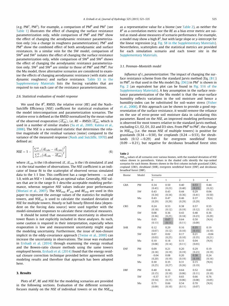
Table 2NSEavg values of all scenarios over various biomes, with the standard deviation of NSEvalues shown in parenthesis. Values in the shaded cells identify the top-rankedscenarios for each biome. Biomes shown in the first column include grassland (GRA),cropland (CRO), shrubland (SHR), evergreen needleleaf forest (ENF) and deciduousbroadleaf forest (DBF).


(e.g. PM1, PM2). For example, a comparison of PM0 and PM1 (seeTable 1) illustrates the effect of changing the surface resistanceparameterization only, while comparison of PM0 and PM2 showthe effect of changing the aerodynamic resistance parameteriza-tion only (via a change in roughness parameterization). PM3 andPM4 show the combined effect of both aerodynamic and surfaceresistances. In a similar vein for the SW model, comparison ofSW0 and SW1 isolates the effect of changing the surface resistanceparameterization only, while comparison of SW0 and SW2 showsthe effect of changing the aerodynamic resistance parameteriza-tion only. SW3 and SW4 are similar to those of PM3 and PM4. Forthe Mu model, three alternative scenarios are considered to exam-ine the effects of changing aerodynamic resistance (with static anddynamic roughness) and surface resistance. Table S3 in theSupplementary Materials lists the forcing variables that arerequired to run each case of the resistance parameterizations.

2.6. Statistical evaluation of model response

We used the R2, RMSD, the relative error (RE) and the Nash–Sutcliffe Efficiency (NSE) coefficient for statistical evaluation ofthe model intercomparison and parameterization scenarios. Therelative error is defined as the RMSD normalized by the mean valueof the observed evaporation (kEobsÞ, i.e. RE ¼ RMSD=kEobs, which isused in a number of similar studies (Su et al., 2005; Kalma et al.,2008). The NSE is a normalized statistic that determines the rela-tive magnitude of the residual variance (noise) compared to thevariance of the measured response (Nash and Sutcliffe, 1970) anddefined as:

NSE ¼ 1�Pn

i¼1 kEi;obs � kEi;sim �2

Pni¼1 kEi;obs � kEobs

�2

24

35 ð6Þ

where kEi;obs is the i th observed kE, kEi;sim is the i th simulated kE andn is the total number of observations. The NSE coefficient is an indi-cator of linear fit to the scatterplot of observed versus simulateddata to the 1:1 line. This coefficient has a range between �1 and1.0, with an NSE = 1 indicating an optimal value. Generally, NSE val-ues that are in the range 0–1 describe acceptable modeling perfor-mance, whereas negative NSE values indicate poor performance(Moriasi et al., 2007). The NSEavg, R2

avg and REavg are used in thispaper to represent the average values of the statistics for multipletowers, and NSEstd is used to calculate the standard deviation ofNSE for multiple towers. Hourly or half-hourly filtered data (depen-dent on the forcing data source) were used together with themodel-simulated responses to calculate these statistical measures.

It should be noted that measurement uncertainty in observedtower fluxes is not explicitly included in these analyses. As such,some caution is required in their interpretation, especially whenevaporation is low and measurement uncertainty might equalthe modeling uncertainty. Furthermore, the issue of non-closureimplicit in the eddy-covariance approach (Twine et al., 2000) canincrease the uncertainty in observations. The issue was evaluatedin Ershadi et al. (2014) through examining the energy residualand the Bowen-ratio closure methods using the same towersemployed herein. Ershadi et al. (2014) found that the energy resid-ual closure correction technique provided better agreement withmodeling results and therefore that approach has been adoptedhere.

3. Results

Plots of R2, RE and NSE for the modeling scenarios are providedin the following sections. Evaluation of the different scenariosfocuses mainly on the NSE of individual towers or on the NSEavg

as a representative value for a biome (see Table 2), as neither theR2 as a correlation metric nor the RE as a bias error metric are sui-ted as stand-alone measures of scenario performance. For example,a model may show a high R2, but with large slope or y-intercept forthe linear regression (e.g. Fig. S8 in the Supplementary Materials).Nevertheless, scatterplots and the statistical metrics are providedfor each simulation scenario and each tower site in theSupplementary Materials.

3.1. Penman–Monteith model

Influence of rs parameterization: The impact of changing the sur-face resistance scheme from the standard Jarvis method (Eq. (B1))in PM0, to that used in the Mu model (Eq. (D6)) in PM1 is shown inFig. 2 (an equivalent bar plot can be found in Fig. S16 of theSupplementary Materials). A key assumption in the surface resis-tance parameterization of the Mu model is that the near-surfacehumidity reflects variations in the soil moisture and hence ahumidity-index can be substituted for soil–water stress (Fisheret al., 2008). If this approach can be shown to provide a good rep-resentation of the surface resistance, it would remove the relianceon the use of error-prone soil moisture data in calculating thisparameter. Based on the NSE, an improved modeling performanceis observed for most towers relative to the standard Jarvis method,excluding G1, E2, D1, D2 and D3 sites. From PM0 to PM1, the changein NSEavg (i.e. the mean NSE of multiple towers) is positive forgrasslands (0.34 ? 0.50), for croplands (0.24 ? 0.53), for shrub-lands (0.12 ? 0.29) and for evergreen needleleaf forest(0.09 ? 0.21), but negative for deciduous broadleaf forest sites

Grassland Cropland Shrubland Evergreen Needleleaf Forest Deciduous Broadleaf Forest

R2

0

0.2

0.4

0.6

0.8

1


RE

0

0.5

1

1.5

2


NSE

-1

-0.5

0

0.5

1

PM0 PM1 PM2 PM3 PM4

PM0 = 0.34PM1 = 0.50PM2 = 0.40PM3 = 0.53PM4 = 0.44

PM0 = 0.24PM1 = 0.53PM2 = 0.38PM3 = 0.57PM4 = 0.55

PM0 = 0.12PM1 = 0.29PM2 = 0.16PM3 = 0.35PM4 = 0.19

PM0 = 0.09PM1 = 0.21PM2 = 0.20PM3 = 0.29PM4 = 0.19

PM0 = 0.40PM1 = 0.36PM2 = 0.64PM3 = 0.52PM4 = 0.60

R2

RE

NSE

Fig. 2. Performance of the Penman–Monteith (PM) model in response to adjusting the resistance parameterization. RE is relative error and NSE is the Nash–Sutcliff efficiency,with each point showing the overall statistic for a particular tower. The x-axis displays the various biomes, with towers in each biome arranged from left to right (e.g. G1 to G4for grassland). The numbers at the bottom of the NSE plot reflect the average NSE (i.e. NSEavg) of the different scenarios for each biome type.


(0.40 ? 0.36). Among grassland, cropland, shrubland and ever-green needleleaf forest biomes, the improvement in NSE is moreevident for cropland sites, where the range in NSE is increased from0.07–0.44 to 0.42–0.65 and the range in RMSD is reduced from107–126 W m�2 to 75–103 W m�2 (see Figs. S1, S4, S7, S10 andS13 in the Supplementary Materials for statistics). Comparison ofPM2 with PM3 (changing Jarvis rs to Mu rs) confirms a similarresponse of trends in NSEavg across the biomes.

Influence of ra parameterization: The influence of dynamic versusstatic roughness on modeling performance can be tracked in com-parisons of two sets of scenarios: PM2 and PM0, and PM3 and PM1.In PM2, adjusting the aerodynamic resistance parameterization viathe use of dynamic roughness values only improved modeling per-formance slightly when compared to PM0. This improvement (interms of NSEavg) is more evident for croplands (0.24 ? 0.38) andfor deciduous broadleaf forest sites (0.40 ? 0.64). Improvementsin NSEavg from PM0 to PM2 are smaller for grasslands(0.34 ? 0.40), shrublands (0.12 ? 0.16) and for evergreen needle-leaf forest (0.09 ? 0.20). Likewise, comparing PM3 with PM1 showsthat the NSE at all towers is increased. The results from both sets ofscenarios show the positive effect of adding dynamic roughness tothe single-source PM model structure.

The PM4 is designed to investigate whether the simple lookup-table based aerodynamic parameterization of the Mu model (Eq.(D11)) can be used in the single-source PM model. The benefit ofthis approach is that the method does not require either roughnessparameters or wind speed. Comparison of NSE values of the PM4

with those of the PM3 shows that NSE at most towers is decreasedin PM4, except in deciduous broadleaf forest sites. Therefore, use ofthe lookup table based approach of Mu for ra parameterization isnot recommended if wind and canopy height data are available.However, comparison of PM4 and PM0 shows that in cases wherewind, canopy height and soil moisture data are not available, use

of the Mu based ra and rs parameterizations can increase NSE atmost sites, excluding G1, G3, S2 and E2 sites. This is an importantresult, as these variables are the ones that are most often unavail-able in data poor regions.

The best performing PM scenario: Overall, the PM3 (which usesMu rs and Thom ra) provides the best performance across mostbiomes, except over deciduous broadleaf forest sites where PM2

(which uses Jarvis rs and Thom ra) presents the best outcome.Both PM3 and PM2 utilize Thom’s equation with dynamic rough-ness, which requires reliable wind speed and canopy height data.Results also suggest that the Jarvis method (used in PM2) is suit-able for deciduous broadleaf forest sites, but for other biomes thesimpler Mu model resistance (used in PM3) is more suitable.

3.2. Shuttleworth–Wallace model

Influence of rs parameterization: Fig. 3 and its equivalent bar plot(see Fig. S17 in the Supplementary Materials) illustrate variationsof R2, RE and NSE coefficients for the different SW scenarios. Achange in surface resistance from Jarvis to Mu in SW0 to SW1

had a limited influence on evaporation estimation over grasslandsites (NSEavg remained constant at 0.43), but improved the NSEavg

for cropland (0.08 ? 0.36), evergreen needleleaf forest(�0.04 ? 0.08) and deciduous broadleaf forest sites(�0.37 ? 0.17) and decreased it for shrublands (0.07 ? 0.02).

The effect of change in rs parameterization from Jarvis to Mucan also be evaluated by comparing SW2 and SW3 (which shareThom ra with dynamic roughness). The comparison in terms ofNSEavg shows a similar trend (as observed for SW0 to SW1) for crop-land (0.43 ? 0.48) and for evergreen needleleaf forest sites(0.20 ? 0.38), but different trends across grassland (0.44 ? 0.29),shrubland (0.17 ? 0.21) and deciduous broadleaf forest sites(0.65 ? 0.66). The results identify that for the SW model, the


R2

0

0.2

0.4

0.6

0.8

1


RE

0

0.5

1

1.5

2


NSE

-1

-0.5

0

0.5

1

SW0 SW1 SW2 SW3 SW4

-1.16

2.74

SW0 = 0.43SW1 = 0.43SW2 = 0.44SW3 = 0.29SW4 = 0.04

SW0 = 0.08SW1 = 0.36SW2 = 0.43SW3 = 0.48SW4 = 0.36

SW0 = 0.07SW1 = 0.02SW2 = 0.17SW3 = 0.21SW4 = -0.04

SW0 = -0.04SW1 = 0.08SW2 = 0.20SW3 = 0.38SW4 = 0.24

SW0 = -0.37SW1 = 0.17SW2 = 0.65SW3 = 0.66SW4 = 0.76

R2

RE

NSE

Fig. 3. Performance of the Shuttleworth–Wallace (SW) model in response to adjusting the resistance parameterization. RE is relative error and NSE is the Nash–Sutcliffefficiency, with each point showing the overall statistic for a particular tower. The x-axis displays the various biomes, with towers in each biome arranged from left to right(e.g. G1 to G4 for grassland). The numbers at the bottom of the NSE plot reflect the average NSE (i.e. NSEavg) of the different scenarios for each biome type. The RE for S2 towerin the SW4 scenario and NSE for D4 tower in the SW0 scenario are out of range, so their values are included on the plot.


influence of rs parameterization is impacted by the influence of thechoice of ra parameterization. As such, parameterizing resistancesfor the SW model should be undertaken with care. Overall, achange in surface resistance had less impact on the modeling effi-ciency of the SW model structure when compared to that observedfor the single-source PM model (see Fig. 2).

Influence of ra parameterization: For aerodynamic resistance,comparisons include evaluating the impact of changes from theSG90 ra to the Thom ra with dynamic roughness (SW0 ? SW2 andSW1 ? SW3), from SG90 ra to the Mu ra (SW1 ? SW4), and fromThom ra with dynamic roughness to Mu ra (SW3 ? SW4).

Compared to SW0, employing Thom’s equation with dynamicroughness in SW2 slightly improved the NSEavg for grasslands(0.43 ? 0.44), considerably increased it for cropland(0.08 ? 0.43), shrubland (0.07 ? 0.17) and evergreen needleleafforest sites (�0.04 ? 0.20) and dramatically improved it for decid-uous broadleaf forest sites (�0.37 ? 0.65). The larger positiveresponse to the changes in ra parameterization in the croplandand the deciduous broadleaf forest sites can be related to the struc-ture of those canopies. That is, the Thom ra equation with dynamicroughness is better able to represent the aerodynamic transfer pro-cesses when full canopy and soil/understory layers are verticallyrepresented and interact in series as in the SW model structure.

For application of the Mu ra in the SW model, comparison ofSW1 (Mu rs, SG90 ra) with SW4 (Mu rs, Mu ra) shows that theNSEavg is decreased for grasslands (0.43 ? 0.04) and shrublands(0.02 ? �0.04), remained constant at 0.36 for croplands, butis significantly increased for evergreen needleleaf forest sites(0.08 ? 0.24) and for deciduous broadleaf forest sites(0.17 ? 0.76). Also, a change of Thom ra with dynamic roughnessin SW3 to Mu ra in SW4 confirms a decrease in NSEavg for a majorityof the towers, except for deciduous broadleaf forest sites where itincreases (0.66 ? 0.76).

Overall, Thom ra with dynamic roughness (used in SW2 andSW3) performed best over grassland, cropland, shrubland and ever-green needleleaf forest sites, while Mu ra performed best overdeciduous broadleaf forest sites.

Influence of using Mu resistance parameterizations: Comparison ofSW4 and SW0 was designed to identify whether a simpler and lessdata demanding resistance parameterization (i.e. using both rs andra from the Mu model) can be usefully employed in flux estimation.Results show that such a parameterization is effective in increasingthe NSEavg across deciduous broadleaf forest sites (�0.37 ? 0.76),evergreen needleleaf forest sites (�0.04 ? 0.24) and croplands(0.08 ? 0.36). However, the performance is degraded across grass-lands (0.43 ? 0.04) and shrublands (0.07 ? �0.04). As such, theuse of the SW4 configuration is not advised for grasslands andshrublands.

The best performing SW scenarios: Among the studied biomes, theSW2 has the best performance over grasslands (marginal improve-ment over SW0 and SW1), while SW4 has the best performance overdeciduous broadleaf forest sites. For other biomes, SW3 is the bestoption. The use of the Mu surface resistance in SW3 and SW4 relaxesthe need for soil moisture data. In contrast, the use of the Jarvis sur-face resistance in SW2 demands reliable soil moisture data. Also,application of the Mu ra parameterization for deciduous broadleafforest sites in SW4 removes the need for wind and canopy heightdata. However, accurate wind speed and canopy height data arerequired for SW2 and SW3, both of which use Thom ra.

3.3. Mu Model

Influence of ra parameterization: Fig. 4 and its equivalent bar plot(see Fig. S18 in the Supplementary Materials) indicate that fromMu0 to Mu1 the NSEavg is increased for grassland (0.43 ? 0.47),cropland (0.65 ? 0.67), shrubland (0.10 ? 0.18) and evergreen


R2

0

0.2

0.4

0.6

0.8

1


RE

0

0.5

1

1.5

2


NSE

-1

-0.5

0

0.5

1

Mu0 Mu1 Mu2 Mu3

Mu0 = 0.43Mu1 = 0.47Mu2 = 0.46Mu3 = 0.37

Mu0 = 0.65Mu1 = 0.67Mu2 = 0.64Mu3 = 0.50

Mu0 = 0.10Mu1 = 0.18Mu2 = 0.15Mu3 = 0.04

Mu0 = 0.30Mu1 = 0.35Mu2 = 0.31Mu3 = 0.15

Mu0 = 0.71Mu1 = 0.66Mu2 = 0.54Mu3 = 0.70

R2

RE

NSE

Fig. 4. Performance of the Mu model in response to adjusting the resistance parameterization. RE is relative error and NSE is the Nash–Sutcliff efficiency, with each pointshowing the overall statistic for a particular tower. The x-axis displays the various biomes, with towers in each biome arranged from left to right (e.g. G1 to G4 for grassland).The numbers at the bottom of the NSE plot reflect the average NSE (i.e. NSEavg) of the different scenarios for each biome type.


needleleaf forest sites (0.30 ? 0.35), but is decreased for deciduousbroadleaf forest sites (0.71 ? 0.66). As such, Thom ra with dynamicroughness slightly improves the performance of the model, exceptover deciduous broadleaf forest sites. Comparison of Mu0 to Mu2

(changing Mu ra to Thom ra with static roughness) shows a similarresponse of trends in NSEavg, but smaller in magnitude, across thebiomes. These results suggest that the change in aerodynamicresistance in the Mu model has a relatively small influence onthe modeling performance, except for deciduous broadleaf forestsites.

Influence of rs parameterization: Compared to Mu0, which usesthe Mu surface resistance, application of the Jarvis surface resis-tance in the Mu3 produced lower values of NSE, except for S1, E2and D1 towers. In particular, the NSEavg is decreased over croplands(0.65 ? 0.50) and evergreen needleleaf forest sites (0.30 ? 0.15).However, change in NSEavg was marginal over deciduous broadleafforest sites (0.71 ? 0.70). Overall, the use of Mu rs provides morerobust flux estimation than does the use of the Jarvis method overa majority of the studied biomes. Such findings are important inthe application of the Mu model in data sparse regions, whereaccurate soil moisture data are not available.

The best performing Mu scenario: The Mu1 scenario has the high-est NSEavg over grassland, cropland, shrubland and evergreenneedleleaf forest sites, and the Mu0 has the highest NSEavg fordeciduous broadleaf forest sites. When accurate wind speed dataor roughness parameters are not available, Mu0 can be used as areplacement for Mu1 with a small compromise in estimation effi-ciency, as the changes in NSEavg from Mu0 to Mu1 were relativelysmall. Mu0 also performed better than Mu3 (Jarvis rs, Mu ra), exceptover deciduous broadleaf forest sites where the performance wassimilar.

3.4. Identification of the best performing models andparameterizations

To develop an overall understanding on the performance of thereviewed scenarios, the NSEavg and NSEstd of each scenario for eachbiome were calculated (see Table 2). From this table it can be seenthat the best performing scenario for grassland and shrubland sitesis PM3, for croplands it is Mu1, for evergreen needleleaf forest sitesit is SW3 and for deciduous broadleaf forest sites it is SW4. In all ofthese scenarios (PM3, Mu1, SW3, SW4) the surface resistance isbased on the Mu method, which requires no soil moisture data.Of the selected top performing scenarios, the Mu ra method is onlyused in SW4 (best performing in the deciduous broadleaf forestsites). However, in the PM3, SW3 and Mu1 scenarios the aerody-namic resistance is calculated using Thom’s equation withdynamic roughness, which requires reliable wind and canopyheight data. As these forcing data are not always available forlarge-scale applications, an important question is to determinewhether the scenarios that use Mu ra over grassland, cropland,shrubland and evergreen needleleaf forest sites can produceNSEavg values close to the top performing model?

To answer this, inspection of the NSEavg and NSEstd values inTable 2 shows that for croplands, Mu0 satisfies the above constraint(0.65 compared to 0.67 for the top model). However, for grasslandsites the next best scenario is PM1 (NSEavg = 0.50), which relies onthe Thom ra formulation. Likewise, no highly ranked alternativescenario can be found for the shrubland and evergreen needleleafforest sites. As such, there are no alternative candidate scenariosfor grassland, shrubland and evergreen needleleaf forest biomesthat produce NSEavg values comparable to those realized from thetop-performing scenarios (see Table 2) by substituting the Mu ra

in the models.


4. Discussion

In the present study, fourteen different scenarios were con-structed to examine how changes in the default resistance param-eterizations of a single-source, a two-layer and a three-source PMtype model might influence their performance in the reproductionof actual evaporation. Intercomparison of these scenarios providedinsights into the influence of both model structure andparameterizations.

4.1. Impact of changes in model structure

Influence of ra parameterization: The aerodynamic resistanceplayed a relatively minor role in flux estimation for the PM model,in accord with the findings of Bailey and Davies (1981) and Irmakand Mutiibwa (2010). Likewise, changes in the aerodynamic resis-tance in the Mu scenarios produced only minor improvements inmodel performance. In contrast, parameterization of the aerody-namic resistance had a major influence on the performance ofthe SW scenarios. Comparison of the various ra schemes in thePM, SW and Mu models indicated that while the Thom ra withdynamic roughness, which requires wind speed and canopy heightdata, increased the NSEavg over a majority of the studied biomes,the performance advantage relative to using the Mu ra was gener-ally marginal for the PM and Mu models. Where wind speed andcanopy height data are available, Thom ra with dynamic roughnessis recommended for the SW model, except over the deciduousbroadleaf forest biome.

Influence of rs parameterization: Analysis of the scenarios illus-trated that the surface resistance parameterization significantlyaffects model performance in the PM and Mu models, while theSW models showed variable responses. For the PM scenarios, theMu rs increased the overall performance (i.e. NSEavg) in croplands,and to a lesser extent in shrubland, evergreen needleleaf forestand in grassland sites. However, it did not improve the results inthe deciduous broadleaf forest sites. The response of the Mu modelto a change in surface resistance parameterization was somewhatdifferent. In the Mu scenarios, the default rs parameterization per-formed better than that of the Jarvis method, except over decidu-ous broadleaf forest sites where the performance change wasmarginal. Nevertheless, pre-calibration of Mu rs might have con-tributed in the increased efficiency of the scenarios that employthose parameters, especially as 11 towers that were used in thecurrent study overlap with those in the Mu et al. (2011) study.

The top-ranked model and parameterizations: Overall, the top-ranked scenarios (see Table 2) for each biome were: PM3 for grass-lands (0.53) and shrublands (0.35), Mu1 for croplands (0.67), SW3

for evergreen needleleaf forest (0.38) and SW4 for deciduousbroadleaf forest sites (0.76) (NSEavg shown in parenthesis). Theseresults highlight the role of model structure in evaporation model-ing, as the single source PM model provided better results overshort canopies (grasslands and shrublands) and the two-layerstructure of the SW model provided better results over forestbiomes. Interestingly, the three-source Mu model structure pro-vided an exception here, as it performed the best when appliedover croplands (which have relatively short canopies).

The common element of the top-ranked scenarios is the use ofthe Mu surface resistance. Likewise, PM3, SW3 and Mu1 all use theThom aerodynamic resistance with dynamic roughness, while SW4

uses the Mu ra. The Mu model itself showed low sensitivity to ra

parameterization, while its rs parameterization improved othermodels.

Comparison with alternative process-based evaporation models:The Penman–Monteith model variants of the current study showedvariable performances in evaporation estimation across the

different studied biomes, even when considering the top-rankedconfigurations. In comparison, a number of alternative process-based models have shown superior performance in related studies.Recently, Ershadi et al. (2014) compared four process-based evap-oration models that included the Surface Energy Balance System(SEBS) (Su, 2002), PT–JPL (Fisher et al., 2008), Advection-Aridity(Brutsaert and Stricker, 1979) and a single-source PM model withJarvis rs and Thom ra with dynamic roughness (i.e. similar toPM2). Using the same dataset of the current study, they found thatan ensemble of model responses had the best performance, fol-lowed by the PT–JPL and SEBS. The issue of appropriate modelselection is obviously a key consideration that will ultimately beguided by user experience, data needs and data availability.Nevertheless, adopting a multi-model strategy for flux estimationseems a useful approach in understanding and constraining theuncertainties that emerge from model structure and parameteriza-tion configurations.

4.2. Issues of data uncertainty

As discussed above, a consideration in the choice of both themodel and parameterization scheme is the availability of reliabledata. Application of the surface resistance method of the Mu modelis important in relaxing the need for soil moisture data and is likelyto facilitate its application in evaporation estimation from field tolarger scales (Mu et al., 2012). Similar results were found in previ-ous work using a modified Priestly–Taylor model (PT–JPL model;Fisher et al., 2008). Like the Mu model, the PT–JPL approach doesnot require wind speed or soil moisture data, and recent compar-isons against more complex models illustrated that the PT–JPL per-forms well (Vinukollu et al., 2011; Ershadi et al., 2014).

The aerodynamic resistance scheme used by the top-ranked sce-narios examined here (except for deciduous broadleaf forest sites)were all based on Thom ra with dynamic roughness, which requiresreliable wind speed and canopy height data. Generally, accurate in-situ based wind speed data are not routinely available for manystudy sites. Likewise, the only source for canopy height at the globalscale is a static product developed by NASA-JPL (Simard et al., 2011),which has limited capability over short vegetation (e.g. grasslandsand croplands). Although the Mu model is designed for large scaleapplications with coarse spatial (1 km) and temporal (8 day toyearly) resolutions, the results of the current study show that inthe absence of required forcing data the Mu resistance scheme couldbe used at the tower scale with reasonable performance.

Part of the deficiencies in model performance, especially overshrubland sites (NSEavg < 0.34) is likely related to the spatio-tem-poral resolution (i.e. 250 m, 16 days) of the MODIS data. MODISdata are used in the estimation of vegetation indices, which aresubsequently used for parameterization of aerodynamic and sur-face resistances. Shrubland sites display considerable land surfaceheterogeneity and the contrasting bare soil and vegetation ele-ments may not be well captured at the coarse remote sensing pix-els (Stott et al., 1998; Montandon and Small, 2008). A differencebetween the results of this and previous studies that have reportedhigher performance of PM type models, may reflect the inherentuncertainties introduced via the input data, since the majority ofprior investigations were performed with detailed field observa-tions of vegetation characteristics (Huntingford et al., 1995; Liet al., 2011). Clearly there is a need for high-quality in-situ pheno-logical descriptions to undertake the types of globally distributedanalysis performed here, but unfortunately they are often lacking.Likewise, a better understanding of the inherent scale issues in fluxestimation is required, particularly for the impact of both spatialand temporal scaling on the performance of aerodynamic and sur-face resistance terms (McCabe and Wood, 2006; Ershadi et al.,2013).


5. Conclusion

The influence of model structure and resistance parameteriza-tion is an important, but often overlooked, consideration in theperformance of Penman–Monteith type evaporation models.Understanding the effects of model structure and parameterizationconfigurations is non-trivial due to the mixed influenceof data uncertainty, hydrometeorological variability and thecomplexity of the modeling system (Raupach and Finnigan,1988). In this study, the effects of model structure and choiceof resistance parameterization were investigated using threePenman–Monteith type models. The structure of the models variedfrom single-source, to two-layer and three-source. To examine theinfluence of model parameterization, a number of commonlyused resistance schemes were substituted into the models, withflux estimates evaluated against locally measured evaporation ata number of eddy-covariance tower sites.

Results illustrated the considerable variability in model perfor-mance over the different biomes, with no single model structure orscenario providing a consistently top-ranked result over thetwenty study sites. Indeed, the top-ranked scenarios highlightedthe importance of model structure. Except over croplands, wherethe three-source Mu model structure performed the best, the sin-gle-source PM structure performed better over short canopieswhile the two-layer SW structure performed better over forestcanopies. Changes in resistance parameterizations, in particularthe surface resistance, were also seen to strongly influence the per-formance of the models.

A key consideration from the findings of this work relates to theapplication of Penman–Monteith type models across a range ofhydrological and related disciplines. Penman–Monteith typeapproaches have been used with modifications in structure andparameterizations in a number of global scale datasets (Zhanget al., 2010), global circulation models (Dolman, 1993) and landsurface model applications. Hence, uncertainties and errors origi-nating from non-optimum structure or parameterization of themodels can significantly influence the accuracy of simulationresults, evaluation of global trends (Jiménez et al., 2011; Muelleret al., 2013) and decisions based on such results, including butnot limited to drought (Sheffield and Wood, 2008), land–atmo-sphere interactions (Seneviratne et al., 2006) and climate changeprojections (Droogers et al., 2012).

As the focus of this paper was on reporting biome-level effi-ciency of model and parameterization configurations, the influenceof vegetation phenology (e.g. LAI, fractional vegetation cover), landcover and climate zone were not explicitly considered in the anal-ysis. Future work is needed to focus on site-level evaluation of themodels to address these important issues. Furthermore, given thatthe top-ranked scenarios identified in this study varied across dif-ferent biomes, an ensemble model based assessment might be anappropriate approach for global flux estimation (Jiménez et al.,2011; Mueller et al., 2011, 2013). Alternatively, a biome-specifictiled evaporation product could also be developed by using thebest model and parameterization configuration for each biometype. In either case, further understanding the role of parameteri-zation on model performance is critical in assessing the impactof choice on derived products.

Acknowledgements

Funding for this research was provided via an AustralianResearch Council (ARC) Linkage (LP0989441) and Discovery(DP120104718) project, together with a top-up scholarship to sup-port Dr Ali Ershadi from the National Centre for GroundwaterResearch and Training (NCGRT) in Australia during his PhD.

Research reported in this publication was also supported by theKing Abdullah University of Science and Technology (KAUST). Wethank the FLUXNET site investigators for allowing the use of theirmeteorological data. This work used eddy-covariance data acquiredby the FLUXNET community and in particular by the AmeriFlux (U.S.Department of Energy, Biological and Environmental Research,Terrestrial Carbon Program: DE-FG02-04ER63917 and DE-FG02-04ER63911) and OzFlux programs. We acknowledge the financialsupport to the eddy-covariance data harmonization provided byCarboEuropeIP, FAO-GTOS-TCO, iLEAPS, Max Planck Institute forBiogeochemistry, National Science Foundation, University ofTuscia, Université Laval and Environment Canada and USDepartment of Energy and the database development and technicalsupport from Berkeley Water Centre, Lawrence Berkeley NationalLaboratory, Microsoft Research eScience, Oak Ridge NationalLaboratory, University of California – Berkeley, University ofVirginia. Data supplied by T. Kolb, School of Forestry, NorthernArizona University, for the US-Fuf site was supported bygrants from the North American Carbon Program/USDA NRI(2004-35111-15057; 2008-35101-19076), Science FoundationArizona (CAA 0-203-08), and the Arizona Water Institute. Matlabscripts for automatic extraction of NDVI time series at towers wereprovided by Dr Tristan Quaife, University College London via theweb portal at http://daac.ornl.gov/MODIS/MODIS-menu/modis_webservice.html.

Appendix A. Details of the selected eddy-covariance towers

See Table A1.

Appendix B. Jarvis surface resistance parameterization method

The Jarvis method for estimation of surface resistance (rs) can beexpressed as:

rs ¼rmin

s

LAI � F1 � F2 � F3 � F4ðB1Þ

where rmins is the minimum canopy resistance (s m�1), LAI is the leaf

area index (m2 m�2) and F1, F2, F3 and F4 are weighting functionsrepresenting the effects of solar radiation, humidity, soil moistureand air temperature on plant stress. Following Chen and Dudhia(2001), the weighting functions for Jarvis method type surface resis-tance are defined as following:

F1 ¼rmin

s =rmaxs þ f

1þ fwith f ¼ 0:55

Rg

Rgl

2LAI

� �

F2 ¼1

1þ hsðq� � qÞF3 ¼ 1� 0:0016ðTref � TaÞ2

F4 ¼XNroot

i¼1

ðhi � hwiltÞdi

ðhref � hwiltÞdt

ðB2Þ

where rmaxs is the maximum canopy resistance (s m�1), Rgl is the

minimum solar radiation necessary for transpiration (W m�2), Rg

is the incident solar radiation (W m�2), hs is a parameter associatedwith the water vapor deficit, q⁄ � q represents the water vapor def-icit (kg kg�1), q⁄ is saturation specific humidity, q is actual specifichumidity, Tref is the optimal temperature for photosynthesis (K)and Ta is the air temperature (K). di is the thickness of the i th soillayer (m), dt is the total thickness of the soil layer (m) and Nroot isthe number of soil layers. In this study, the observation depth ofthe soil moisture sensor(s) (5–10 cm) is considered to be represen-tative of the overall soil column. Obviously, there is potential forrapid changes in the observed near-surface soil moisture (as a

http://daac.ornl.gov/MODIS/MODIS-menu/modis_webservice.html

http://daac.ornl.gov/MODIS/MODIS-menu/modis_webservice.html

Table A1Selected eddy-covariance towers and their characteristics (Ershadi et al., 2014). zg is the site elevation (above sea level) in m, zm is tower height in m, hc is the canopy height in m,Y is the number of years of data and L is the processing level of data. Abbreviations for climate types are defined for Sub-Tropical Mediterranean (STM), Temperate Continental(TC), Temperate (TEM) and Tropical (TRO).

ID Name Country Climate Lat. Lon. zg zm hc Y L Reference

GrasslandsG1 PT-Mi2 Mitra IV Tojal Portugal STM 38.5 �8.0 190 2.5 0.05 2 3 Gilmanov et al. (2007)G2 US-Aud Audubon Research Ranch USA Dry 31.6 �110.5 1469 4 0.15 4 3 Krishnan et al. (2012)G3 US-Goo Goodwin Creek USA STM 34.3 �89.9 87 4 0.3 4 3 Hollinger et al. (2010)G4 US-Fpe Fort Peck USA Dry 48.3 �105.1 634 3.5 0.3 4 3 Horn and Schulz (2011)

CroplandsC1 US-ARM ARM SGP – Lamont USA STM 36.6 �97.5 314 60 0.5 4 3 Lokupitiya et al. (2009)C2 US-Ne3 Mead – rainfed USA TC 41.2 �96.4 363 6 2.5 10 3 Richardson et al. (2006)C3 US-Ne1 Mead – irrigated USA TC 41.2 �96.5 361 6 3 10 3 Richardson et al. (2006)C4 US-Bo1 Bondville USA TC 40.0 �88.3 219 10 3 7 3 Hollinger et al. (2010)

Shrubland/woody savannahS1 US-SRc Santa Rita Creosote USA Dry 31.9 �110.8 991 4.25 1.7 1.5 2 Cavanaugh et al. (2011)S2 US-SRM Santa Rita Mesquite USA Dry 31.8 �110.9 1116 6.4 2.5 7 2 Scott et al. (2009)S3 BW-Ma1 Maun – Mopane Woodland Botswana Dry �19.9 23.6 950 13.5 8 2 3 Veenendaal et al. (2004)S4 AU-How Howard Springs Australia TRO �12.5 131.2 38 23 15 5 3 Hutley et al. (2005)

Evergreen needleleaf forestE1 NL-Loo Loobos Netherlands TEM 52.2 5.7 25 52 15.9 5 3 Sulkava et al. (2011)E2 US-Fuf Flagstaff – Unmanaged Forest USA TC 35.1 �111.8 2180 23 18 6 2 Román et al. (2009)E3 DE-Tha Anchor St. Tharandt – old spruce Germany TEM 51.0 13.6 380 42 30 2 3 Delpierre et al. (2009)E4 US-Wrc Wind River Crane Site USA TEM 45.8 �122.0 371 85 56.3 9 2 Wharton et al. (2009)

Deciduous broadleaf forestD1 US-MOz Missouri Ozark Site USA STM 38.7 �92.2 219 30 24.2 5 2 Hollinger et al. (2010)D2 US-WCr Willow Creek USA TC 45.8 �90.1 520 30 24.3 5 3 Curtis et al. (2002)D3 US-MMS Morgan Monroe State Forest USA STM 39.3 �86.4 275 48 27 6 2 Dragoni et al. (2011)D4 DE-Hai Hainich Germany TEM 51.1 10.5 430 43.5 33 3 3 Rebmann et al. (2005)


response to precipitation) which may not accurately reflect the dee-per soil column response, especially for sites with deeply rootedsystem. However, as there is limited availability of soil moisturedata with which to refine the technique, we employ this relativelysimple scheme as a compromise. The G1, S3, S4, E1, E3 and D4 tow-ers (see Table A1) had one soil layer, and the rest of towers had twosoil layers included in the analysis. Values of rmin

s , rmaxs , Rgl, hs and Tref

were based on the vegetation lookup tables used in the NOAH landsurface model (see Kumar et al., 2011).

Soil moisture content thresholds for field capacity (href) andwilting point (hwilt) provide characteristics of the soil type. As soiltype information is not available for all sites from field investiga-tions and the values in existing global soil databases are not reli-able at the point scale, long-term surface layer soil moistureobservations from each tower are used to determine soil moisturethresholds (Calvet et al., 1998; Zotarelli et al., 2010). To do this, thefield capacity is determined as the 99th percentile of the ‘‘afterrain’’ soil moisture records of the tower. The estimated href is con-strained by the maximum value of href in the NOAH soil table, asthe length of soil moisture data might not be sufficient to resulta realistic href. Similarly, the wilting point threshold is determinedfrom the 1st percentile of the soil moisture records, but capped tothe minimum value of hwilt in the NOAH soil table. Both vegetationand soil parameter tables of the NOAH model can be obtained fromhttp://www.ral.ucar.edu/research/land/technology/lsm.php.

Appendix C. Shuttleworth–Wallace model

In the SW model, Cc and Cs are resistance functions for canopyand soil (respectively) and are given by the following equations:

Cc ¼ 1þ RcRa

RsðRc þ RaÞ

� ��1

ðC1Þ

Cs ¼ 1þ RsRa

RcðRs þ RaÞ

� ��1

ðC2Þ

where

Ra ¼ ðDþ cÞraa ðC3Þ

The bulk stomatal resistance of the canopy (rcs) is a surface resis-

tance, which is influenced by the surface area of the vegetation. Inthe original derivation of the SW model, the bulk stomatal resis-tance was calculated by upscaling the leaf scale stomatal resistance(rST) based on the leaf area index (LAI) as rc

s ¼ rST=2� LAI, with rST

assumed as a constant value or calibrated based on evaporationobservations. However, we derive the bulk canopy resistance usingthe Jarvis method of Noilhan and Planton (1989) (see Appendix B),as is used in a number of previous studies of the Shuttleworth–Wallace model (e.g. Zhou et al., 2006; Irmak, 2011). The soil surfaceresistance (rs

s) is derived from the above mentioned Jarvis method,using the ‘‘Barren and Sparsely Vegetated’’ category of the NOAHvegetation table for the bare soil.

Three aerodynamic resistances appear in the SW model: anaerodynamic resistance between the soil/substrate surface andthe canopy source height (rs

a), a bulk boundary layer resistance ofvegetative elements in the canopy (rc

a), and an aerodynamic resis-tance between the canopy source height and a reference levelabove the canopy (ra

a). The bulk boundary layer resistance (rca) is

calculated by scaling the leaf scale mean boundary layer resistancerb to the canopy scale using LAI, as rc

a ¼ rb=2� LAI, with rb consid-ered constant at 25 s m�1 (Shuttleworth and Wallace, 1985).However, ra

a and rsa are calculated using the following equations

(Shuttleworth and Gurney, 1990) (i.e. SG90):

raa ¼

1ju�

lnz� d0

hc � d0

� �þ hc

nKhexp n 1� z0m þ d0

hc

� �� 1

� ðC4Þ

rsa ¼

hc expðnÞnKh

exp �nz00m

hc

� �� exp �n

z0m þ d0

hc

� �� ðC5Þ

where z00m is the roughness length of bare soil surface (=0.01 m)(van Bavel and Hillel, 1976) and n is the eddy diffusivity decay con-stant (dimensionless), which is assumed fixed at 2.5 for agricultural

http://www.ral.ucar.edu/research/land/technology/lsm.php


crops by Shuttleworth and Wallace (1985). However, followingZhang et al. (2008) and based on the values given by Brutsaert(1982), we assume n = 2.5 when hc < 1 m and n = 4.25 whenhc > 10 m. For the cases where 1 P hc P 10, a linear interpolationis applied as n = 0.1944hc + 2.3056. The eddy diffusion coefficientat the top of canopy (Kh in m2 s�1) is calculated asKh = ju⁄(hc � d0), with the friction velocity (u⁄ in m s�1) calculatedas u⁄ = jua/ln [(z � d0)/z0m]. As is common in general applicationsof the SW model, the roughness variables d0 and z0m are assumedas a fraction of the canopy height (Brutsaert, 2005), as in Eq. (3).

Appendix D. Mu model evaporation component and resistances

D.1. Evaporation from wet canopy

Evaporation from a wet canopy (i.e. intercepted water) is calcu-lated using the following equation:

kEwc ¼ f wDAc þ f cqcpðe� � eÞ=rwc

a

Dþ c rwcs

rwca

ðD1Þ

where fc is fractional vegetation cover. fw is the relative surface wet-ness and calculated as fw = RH4, which is based on the concept orig-inally developed by Fisher et al. (2008). In the original Mu model,daily average values of RH were used and fw was assumed zerowhen daily average RH < 0.7. However, here we used hourly (orhalf-hourly) data and did not filter fw based on low RH values.

The aerodynamic resistance rwca and surface resistance rwc

s forwet canopy are defined as:

rwca ¼

rwch rwc

r

rwch þ rwc

rðD2Þ

rwcs ¼

1f wgeLAI

ðD3Þ

where rwch is wet canopy resistance to sensible heat transfer and rwc

r

is the wet canopy resistance to radiative heat transfer, which areformulated as following:

rwch ¼

1f wghLAI

rwcr ¼

qcp

4rT3a

ðD4Þ

ge and gh are leaf conductance to evaporated water vapor and sen-sible heat (respectively) per unit LAI, Ta is air temperature (�C) and ris the Stefan–Boltzmann constant. Based on Mu et al. (2011), ge andgh are assumed similar and constant for each biome as listed inTable B1. The available energy for crop and soil is partitioned basedon the fractional vegetation cover (fc) as Ac = fcRn andAs = (1 � fc)Rn � G0.

D.2. Canopy transpiration

The canopy transpiration kEt is calculated as:

kEt ¼ ð1� f wÞDAc þ f cqcpðe� � eÞ=rt

a

Dþ c 1þ rts

rta

� � ðD5Þ

where rta and rt

s are aerodynamic and surface resistances for transpi-ration, respectively. The bulk canopy resistance (rt

s) is the inverse ofthe bulk canopy conductance (Cc) and calculated as:

rts ¼

1Cc

ðD6Þ

The assumption here is that the stomatal conductance (Gsts ) and

cuticular conductance (Gcus ) are in parallel, but both are in series

with the canopy boundary-layer conductance Gbs . Therefore, the

canopy conductance to transpiration is calculated as:

Cc ¼ð1� f wÞ

ðGsts þGcu

s ÞGbs

Gsts þGcu

s þGbsLAI; LAI > 0; ð1� f wÞ > 0

0; LAI ¼ 0; ð1� f wÞ ¼ 0

8<: ðD7Þ

where Gbs ¼ gh, Gcu

s ¼ rcorrgcu and Gsts ¼ cLmðTminÞmðVPDÞrcorr with

VPD being the vapor pressure deficit (Pa). The leaf cuticular conduc-tance (gcu) is per unit LAI, and assumed equal to 0.00001 m s�1 forall biomes. Also, the mean potential stomatal conductance (cL) isper unit leaf area, and is assumed constant for each biome(Table B1). The rcorr is the correction factor for Gst

s to adjust it basedon the standard air temperature and pressure (20 �C and101,300 Pa) using the following equation:

rcorr ¼1

101300Pa

Ta þ 273:15293:15

� �1:75 ðD8Þ

m(Tmin) is a multiplier that limits potential stomatal conductance byminimum air temperature (Tmin), and m(VPD) is a multiplier used toreduce the potential stomatal conductance when VPD = e⁄ � e ishigh enough to reduce canopy conductance. Following Mu et al.(2007), m(Tmin) and m(VPD) are calculated as following:

mðTminÞ ¼

1 Tmin P Topenmin

Tmin � Tclosemin

Topenmin � Tclose

min

Tclosemin < Tmin < Topen

min

0 Tmin 6 Tclosemin

8>>>><>>>>:

ðD9Þ

mðVPDÞ ¼

1 VPD 6 VPDopen

VPDclose � VPDVPDclose � VPDopen

VPDopen < VPD < VPDopen

0 VPD P VPDclose

8>>><>>>:

ðD10Þ

Values of Topenmin , Tclose

min , VPDopen and VPDclose are listed in Table B1 foreach biome type. Also, the aerodynamic resistance to canopy tran-spiration, rt

a, is calculated based on the convective heat transferresistance rh and radiative heat transfer resistance rr, assuming theyare in parallel using the following equation (Thornton, 1998):

rta ¼

rthrt

r

rth þ rt

rðD11Þ

where rth ¼ 1=gbl and rt

r ¼ rwcr with gbl being the leaf-scale boundary

layer conductance per unit LAI and assumed equal to that of thesensible heat (i.e. gbl = gh).

D.3. Soil evaporation

Evaporation from the soil surface is calculated as the sum ofevaporation from wet soil (kEws) and evaporation from saturatedsoil (kEss), such that:

kEs ¼ kEws þ kEss: ðD12Þ

Partitioning of the soil surface to wet and saturated components isbased on the relative surface wetness fw, with the evaporation fromthe wet soil calculated as:

kEws ¼ f wDAs þ ð1� f cÞqcpðe� � eÞ=rs

a

Dþ c rss

rsa

: ðD13Þ

Similarly, evaporation from the saturated soil is calculated as:

kEss ¼ RHVPD=bð1� f wÞDAs þ ð1� f cÞqcpðe� � eÞ=rs

a

Dþ c rss

rsa

Table B1The Biome-Property-Lookup-Table (BPLT) adopted from Mu et al. (2011). Land covers are defined as evergreen needleleaf forest (ENF), evergreen broadleaf forest (EBF), deciduousneedleleaf forest (DNF), deciduous broadleaf forest (DBF), mixed forest (MF), woody savannahs (WL), savannahs (SV), closed shrubland (CSH), open shrubland (OSH) and cropland(CRO). GRA class is for grassland, urban and built-up, and barren or sparsely vegetated biomes, collectively.

Crop ENF EBF DNF DBF MF CSH OSH WL SV GRA CRO

Topenmin (�C) 8.31 9.09 10.44 9.94 9.5 8.61 8.8 11.39 11.39 12.02 12.02

Tclosemin (�C) �8 �8 �8 �6 �7 �8 �8 �8 �8 �8 �8

VPDclose (Pa) 3000 4000 3500 2900 2900 4300 4400 3500 3600 4200 4500VPDopen (Pa) 650 1000 650 650 650 650 650 650 650 650 650gh (m s�1) 0.04 0.01 0.04 0.01 0.04 0.04 0.04 0.08 0.08 0.02 0.02ge (m s�1) 0.04 0.01 0.04 0.01 0.04 0.04 0.04 0.08 0.08 0.02 0.02cL (m s�1) 0.0032 0.0025 0.0032 0.0028 0.0025 0.0065 0.0065 0.0065 0.0065 0.007 0.007rmin

bl (m s�1) 65 70 65 65 65 20 20 25 25 20 20

rmaxbl (m s�1) 95 100 95 100 95 55 55 45 45 50 50


where rsa and rs

s are aerodynamic and surface resistances for the soil

surface. RHVPD=b is a soil moisture constraint that is used followingFisher et al. (2008). This function is based on the complementaryhypothesis and describes land–atmosphere interactions via the airvapor pressure deficit VPD and relative humidity RH, with bassigned a constant value of 200. The soil surface resistance rs

s is cal-culated as:

rss ¼ rcorrrtotc ðD14Þ

where rtotc is a function of VDP and biological parameters rminbl and

rmaxbl as follows:

rtotc ¼

rmaxbl VPD 6 VPDopen

rmaxbl �

rmaxbl�rmin

blð Þ�ðVPDclose�VPDÞVPDclose�VPDopen

VPDopen < VPD < VPDclose

rminbl VPD P VPDclose

8>><>>:

ðD15Þ

VPDopen is the VPD when there is no water stress on transpirationand VPDclose is the VPD when water stress causes stomata to closealmost completely, halting plant transpiration. Values for rmax

bl ,rmin

bl , VPDopen and VPDclose are listed in Table B1.The aerodynamic resistance at the soil surface (rs

a) is parallel toboth the resistance to convective heat transfer (rs

h) and the resis-tance to radiative heat transfer rs

r , with its components calculatedas:

rsa ¼

rshrs

r

rsh þ rs

rðD16Þ

where rsr ¼ rwc

r and rsh ¼ rs

s.Table 2 shows the Biome-Property-Lookup-Table (BPLT) used in

the Mu model. As explained by Mu et al. (2011), VPD and Tmin

parameters were derived from calibrations performed by Zhaoet al. (2005), but other parameters were calibrated based on biomeaggregated observed evaporation and Gross Primary Production(GPP) values at 46 AmeriFlux tower sites, some of which areincluded in the current study.

Appendix E. The dynamic roughness parameterization method

In the Su et al. (2001) method, the roughness height formomentum transfer is calculated as:

z0m ¼ hc 1� d0

hc

� �exp �j

g

� �ðE1Þ

where hc is the canopy height and g is the ratio of friction velocity tothe wind speed at the canopy top, calculated asg = c1 � c2 exp(�c3CdLAI) with c1 = 0.32, c2 = 0.264, c3 = 15.1 andthe drag coefficient Cd = 0.2. The roughness length for heat transfer(z0h) can be derived by assuming an exponential relationship

between z0m and z0h as z0h = z0m/exp(jB�1), where B�1 is the inverseStanton number. To estimate the jB�1 parameter, the method of Suet al. (2001) suggests:

jB�1 ¼ jCd

4Ctb 1� exp � nec2

� � f 2c þ 2f cf s

jgz0m=hc

C�tþ jB�1

s f 2s ðE2Þ

where fc is the fractional canopy coverage and fs is its complement(for soil coverage). Ct is the heat transfer coefficient of the leaf, C�t isthe heat transfer coefficient of the soil and nec is within-canopywind speed profile extinction coefficient.

As noted by Su (2002), the first term of Eq. (E2) follows the fullcanopy model of Choudhury and Monteith (1988), the third term isthat of Brutsaert (1982) for a bare soil surface and the second termdescribes the interaction between vegetation and a bare soil sur-face. Following Brutsaert (1999), for a bare soil surface the jB�1

s

is calculated as jB�1s ¼ 2:46Re1=4

� � lnð7:4Þ with Re⁄ being theReynolds number. More details about the methodology and formu-lation are available in Su et al. (2001) and Su (2002).

Appendix F. Supplementary material

Supplementary data associated with this article can be found, inthe online version, at http://dx.doi.org/10.1016/j.jhydrol.2015.04.008.

References

Allen, R.G., Pereira, L.S., Howell, T.A., Jensen, M.E., 2011. Evapotranspirationinformation reporting: II. Recommended documentation. Agric. WaterManage. 98 (6), 921–929.

Bailey, W.G., Davies, J.A., 1981. The effect of uncertainty in aerodynamic resistanceon evaporation estimates from the combination model. Bound.-Layer Meteorol.20 (2), 187–199.

Baldocchi, D. et al., 2001. FLUXNET: a new tool to study the temporal and spatialvariability of ecosystem-scale carbon dioxide, water vapor, and energy fluxdensities. Bull. Am. Meteorol. Soc. 82 (11), 2415–2434.

Brutsaert, W., 1982. Evaporation into the Atmosphere: Theory, History, andApplications. Reidel Publishing, Dordrecht etc., 299pp.

Brutsaert, W., 1999. Aspects of bulk atmospheric boundary layer similarity underfree-convective conditions. Rev. Geophys. 37.

Brutsaert, W., 2005. Hydrology: An Introduction. Cambridge University Press,Cambridge, 605pp.

Brutsaert, W., Stricker, H., 1979. An advection-aridity approach to estimate actualregional evapotranspiration. Water Resour. Res. 15 (2), 443–450.

Calvet, J.C., Noilhan, J., Bessemoulin, P., 1998. Retrieving the root-zone soil moisturefrom surface soil moisture or temperature estimates: a feasibility study basedon field measurements. J. Appl. Meteorol. 37 (4), 371–386.

Cavanaugh, M.L., Kurc, S.A., Scott, R.L., 2011. Evapotranspiration partitioning insemiarid shrubland ecosystems: a two-site evaluation of soil moisture controlon transpiration. Ecohydrology 4 (5), 671–681.

Chen, F., Dudhia, J., 2001. Coupling an advanced land surface-hydrology model withthe Penn State-NCAR MM5 modeling system. Part I: Model implementation andsensitivity. Mon. Weather Rev. 129 (4), 569–585.

Choudhury, B.J., Monteith, J.L., 1988. A four-layer model for the heat budget ofhomogeneous land surfaces. Q. J. R. Meteorol. Soc. 114 (480), 373–398.



http://refhub.elsevier.com/S0022-1694(15)00257-7/h0005





























Curtis, P.S. et al., 2002. Biometric and eddy-covariance based estimates of annualcarbon storage in five eastern North American deciduous forests. Agric. For.Meteorol. 113 (1), 3–19.

Delpierre, N. et al., 2009. Exceptional carbon uptake in European forests during thewarm spring of 2007: a data–model analysis. Glob. Change Biol. 15 (6), 1455–1474.

Dolman, A.J., 1993. A multiple-source land surface energy balance model for use ingeneral circulation models. Agric. For. Meteorol. 65 (1–2), 21–45.

Dragoni, D. et al., 2011. Evidence of increased net ecosystem productivity associatedwith a longer vegetated season in a deciduous forest in south-central Indiana,USA. Glob. Change Biol. 17 (2), 886–897.

Droogers, P. et al., 2012. Water resources trends in Middle East and North Africatowards 2050. Hydrol. Earth Syst. Sci. 16 (9), 3101–3114.

Ershadi, A., McCabe, M.F., Evans, J.P., Walker, J.P., 2013. Effects of spatial aggregationon the multi-scale estimation of evapotranspiration. Remote Sens. Environ. 131,51–62.

Ershadi, A., McCabe, M.F., Evans, J.P., Chaney, N.W., Wood, E.F., 2014. Multi-siteevaluation of terrestrial evaporation models using FLUXNET data. Agric. For.Meteorol. 187, 46–61.

Ferguson, C.R., Sheffield, J., Wood, E.F., Gao, H., 2010. Quantifying uncertainty in aremote sensing-based estimate of evapotranspiration over continental USA. Int.J. Remote Sens. 31 (14), 3821–3865.

Finnigan, J.J., Clement, R., Malhi, Y., Leuning, R., Cleugh, H.A., 2003. A re-evaluationof long-term flux measurement techniques – Part I: averaging and coordinaterotation. Bound.-Layer Meteorol. 107 (1), 1–48.

Fisher, J.B., DeBiase, T.A., Qi, Y., Xu, M., Goldstein, A.H., 2005. Evapotranspirationmodels compared on a Sierra Nevada forest ecosystem. Environ. Model. Softw.20 (6), 783–796.

Fisher, J.B., Tu, K.P., Baldocchi, D.D., 2008. Global estimates of the land-atmospherewater flux based on monthly AVHRR and ISLSCP-II data, validated at 16FLUXNET sites. Remote Sens. Environ. 112 (3), 901–919.

Foken, T., Leuning, R., Oncley, S.R., Mauder, M., Aubinet, M., 2012. Corrections anddata quality control. In: Aubinet, M., Vesala, T., Papale, D. (Eds.), EddyCovariance, A Practical Guide to Measurement and Data Analysis. Springer.

Gilmanov, T.G. et al., 2007. Partitioning European grassland net ecosystem CO2exchange into gross primary productivity and ecosystem respiration using lightresponse function analysis. Agric. Ecosyst. Environ. 121 (1), 93–120.

Hollinger, D.Y. et al., 2010. Albedo estimates for land surface models and support fora new paradigm based on foliage nitrogen concentration. Glob. Change Biol. 16(2), 696–710.

Horn, J.E., Schulz, K., 2011. Identification of a general light use efficiency model forgross primary production. Biogeosciences 8, 999–1021.

Huntingford, C., Allen, S.J., Harding, R.J., 1995. An intercomparison of single anddual-source vegetation-atmosphere transfer models applied to transpirationfrom Sahelian savannah. Bound.-Layer Meteorol. 74 (4), 397–418.

Hutley, L.B., Leuning, R., Beringer, J., Cleugh, H.A., 2005. The utility of the eddycovariance techniques as a tool in carbon accounting: tropical savanna as a casestudy. Aust. J. Bot. 53 (7), 663–675.

Inclán, M.G., Forkel, R., 1995. Comparison of energy fluxes calculated with thePenman–Monteith equation and the vegetation models SiB and Cupid. J. Hydrol.166 (3–4), 193–211.

Irmak, A., 2011. Evapotranspiration – Remote Sensing and Modeling. InTech,Croatia.

Irmak, S., Mutiibwa, D., 2010. On the dynamics of canopy resistance: generalizedlinear estimation and relationships with primary micrometeorologicalvariables. Water Resour. Res. 46 (8), W08526.

Jacquemin, B., Noilhan, J., 1990. Sensitivity study and validation of a land surfaceparameterization using the HAPEX-MOBILHY data set. Bound.-Layer Meteorol.52 (1), 93–134.

Jiménez, C. et al., 2011. Global intercomparison of 12 land surface heat fluxestimates. J. Geophys. Res. 116 (D2), D02102.

Jiménez-Muñoz, J. et al., 2009. Comparison between fractional vegetationcover retrievals from vegetation indices and spectral mixture analysis:case study of PROBA/CHRIS data over an agricultural area. Sensors 9 (2), 768–793.

Kalma, J., McVicar, T., McCabe, M., 2008. Estimating land surface evaporation: areview of methods using remotely sensed surface temperature data. Surv.Geophys. 29 (4), 421–469.

Krishnan, P., Meyers, T.P., Scott, R.L., Kennedy, L., Heuer, M., 2012. Energy exchangeand evapotranspiration over two temperate semi-arid grasslands in NorthAmerica. Agric. For. Meteorol. 153, 31–44.

Kumar, A. et al., 2011. Evaluation of a photosynthesis-based canopy resistanceformulation in the Noah land-surface model. Bound.-Layer Meteorol. 138 (2),263–284.

Li, L. et al., 2011. Modelling evapotranspiration in a Central Asian desert ecosystem.Ecol. Model. 222 (20–22), 3680–3691.

Lokupitiya, E. et al., 2009. Incorporation of crop phenology in Simple BiosphereModel (SiBcrop) to improve land-atmosphere carbon exchanges fromcroplands. Biogeosciences 6, 1103.

McCabe, M.F., Wood, E.F., 2006. Scale influences on the remote estimation ofevapotranspiration using multiple satellite sensors. Remote Sens. Environ. 105(4), 271–285.

McCabe, M.F., Kalma, J.D., Franks, S.W., 2005. Spatial and temporal patterns of landsurface fluxes from remotely sensed surface temperatures within anuncertainty modelling framework. Hydrol. Earth Syst. Sci. 9 (5), 467–480.

Montandon, L.M., Small, E.E., 2008. The impact of soil reflectance on thequantification of the green vegetation fraction from NDVI. Remote Sens.Environ. 112 (4), 1835–1845.

Monteith, J.L., 1965. Evaporation and environment. Symp. Soc. Exp. Biol. 19, 205–234.

Moriasi, D.N. et al., 2007. Model Evaluation Guidelines for Systematic Quantificationof Accuracy in Watershed Simulations, 50. American Society of AgriculturalEngineers, St. Joseph, MI, ETATS-UNIS, 16pp.

Mu, Q., Heinsch, F.A., Zhao, M., Running, S.W., 2007. Development of a globalevapotranspiration algorithm based on MODIS and global meteorology data.Remote Sens. Environ. 111 (4), 519–536.

Mu, Q., Zhao, M., Running, S.W., 2011. Improvements to a MODIS global terrestrialevapotranspiration algorithm. Remote Sens. Environ. 115 (8), 1781–1800.

Mu, Q., Zhao, M., Kimball, J.S., McDowell, N.G., Running, S.W., 2012. A remotelysensed global terrestrial drought severity index. Bull. Am. Meteorol. Soc. 94 (1),83–98.

Mueller, B. et al., 2011. Evaluation of global observations-based evapotranspirationdatasets and IPCC AR4 simulations. Geophys. Res. Lett. 38 (6), L06402.

Mueller, B. et al., 2013. Benchmark products for land evapotranspiration: LandFlux-EVAL multi-dataset synthesis. Hydrol. Earth Syst. Sci. Discuss. 10 (1), 769–805.

Nash, J.E., Sutcliffe, J.V., 1970. River flow forecasting through conceptual modelspart I—a discussion of principles. J. Hydrol. 10 (3), 282–290.

Noilhan, J., Planton, S., 1989. A simple parameterization of land surface processesfor meteorological models. Mon. Weather Rev. 117 (3), 536–549.

Ortega-Farias, S., Poblete-Echeverría, C., Brisson, N., 2010. Parameterization of atwo-layer model for estimating vineyard evapotranspiration usingmeteorological measurements. Agric. For. Meteorol. 150 (2), 276–286.

Penman, H.L., 1948. Natural evaporation from open water, bare soil and grass. Proc.R. Soc. Lond. A 193 (1032), 120–145.

Raupach, M., Finnigan, J., 1988. Single-layer models of evaporation from plantcanopies are incorrect but useful, whereas multilayer models are correct butuseless. Funct. Plant Biol. 15 (6), 705–716.

Rebmann, C. et al., 2005. Quality analysis applied on eddy covariancemeasurements at complex forest sites using footprint modelling. Theoret.Appl. Climatol. 80 (2–4), 121–141.

Richardson, A.D. et al., 2006. A multi-site analysis of random error in tower-basedmeasurements of carbon and energy fluxes. Agric. For. Meteorol. 136 (1–2), 1–18.

Román, M.O. et al., 2009. The MODIS (Collection V005) BRDF/albedo product:assessment of spatial representativeness over forested landscapes. RemoteSens. Environ. 113 (11), 2476–2498.

Ross, J., 1976. Radiative transfer in plant communities. In: Monteith, J.L. (Ed.),Vegetation and the Atmosphere. Academic Press, London, pp. 13–56.

Scott, R.L., Jenerette, G.D., Potts, D.L., Huxman, T.E., 2009. Effects of seasonal droughton net carbon dioxide exchange from a woody-plant-encroached semiaridgrassland. J. Geophys. Res.: Biogeosci. 114 (G4), G04004.

Seneviratne, S.I., Lüthi, D., Litschi, M., Schär, C., 2006. Land–atmosphere couplingand climate change in Europe. Nature 443 (7108), 205–209.

Sheffield, J., Wood, E., 2008. Projected changes in drought occurrence under futureglobal warming from multi-model, multi-scenario, IPCC AR4 simulations. Clim.Dyn. 31 (1), 79–105.

Shuttleworth, W.J., Gurney, R.J., 1990. The theoretical relationship between foliagetemperature and canopy resistance in sparse crops. Quart. J. Roy. Meteorol. Soc.116 (492), 497–519.

Shuttleworth, W.J., Wallace, J.S., 1985. Evaporation from sparse crops-an energycombination theory. Quart. J. Roy. Meteorol. Soc. 111 (469), 839–855.

Simard, M., Pinto, N., Fisher, J.B., Baccini, A., 2011. Mapping forest canopy heightglobally with spaceborne lidar. J. Geophys. Res.: Biogeosci. 116 (G4), G04021.

Solano, R., Didan, K., Jacobson, A., Huete, A., 2010. MODIS Vegetation Index User’sGuide, Vegetation Index and Phenology Lab. The University of Arizona.

Stannard, D.I., 1993. Comparison of Penman–Monteith, Shuttleworth-Wallace, andModified Priestley–Taylor Evapotranspiration Models for wildland vegetation insemiarid rangeland. Water Resour. Res. 29 (5), 1379–1392.

Stott, P., Paruelo, J.M., Lauenroth, W.K., 1998. Interannual variability of NDVI and itsrelationship to climate for North American shrublands and grasslands. J.Biogeogr. 25 (4), 721–733.

Su, Z., 2002. The Surface Energy Balance System (SEBS) for estimation of turbulentheat fluxes. Hydrol. Earth Syst. Sci. 6 (1), 85–100.

Su, Z., Schmugge, T., Kustas, W.P., Massman, W.J., 2001. An evaluation of two modelsfor estimation of the roughness height for heat transfer between the landsurface and the atmosphere. J. Appl. Meteorol. 40 (11), 1933–1951.

Su, H., McCabe, M.F., Wood, E.F., Su, Z., Prueger, J.H., 2005. Modelingevapotranspiration during SMACEX: comparing two approaches for local- andregional-scale prediction. J. Hydrometeorol. 6 (6), 910–922.

Sulkava, M., Luyssaert, S., Zhehle, S., Papale, D., 2011. Assessing and improving therepresentativeness of monitoring networks: the European flux tower networkexample. J. Geophys. Res. 116.

Tan, B. et al., 2006. The impact of gridding artifacts on the local spatial properties ofMODIS data: implications for validation, compositing, and band-to-bandregistration across resolutions. Remote Sens. Environ. 105 (2), 98–114.

Thom, A.S., 1975. Momentum, mass and heat exchange of the plant communities.In: Monteith, J.L. (Ed.), Vegetation and Atmosphere. Academic Press, London, pp.57–109.

Thornton, P.E., 1998. Regional ecosystem simulation: combining surface- andsatellite-based observations to study linkages between terrestrial energy and










































































































































































mass budgets. 9828151 Thesis. University of Montana, Montana, United States,pp. 280–280.

Twine, T.E. et al., 2000. Correcting eddy-covariance flux underestimates over agrassland. Agric. For. Meteorol. 103 (3), 279–300.

van Bavel, C.H.M., Hillel, D.I., 1976. Calculating potential and actual evaporationfrom a bare soil surface by simulation of concurrent flow of water and heat.Agric. Meteorol. 17 (6), 453–476.

Veenendaal, E.M., Kolle, O., Lloyd, J., 2004. Seasonal variation in energy fluxes andcarbon dioxide exchange for a broad-leaved semi-arid savanna (Mopanewoodland) in Southern Africa. Glob. Change Biol. 10 (3), 318–328.

Vinukollu, R.K., Wood, E.F., Ferguson, C.R., Fisher, J.B., 2011. Global estimates ofevapotranspiration for climate studies using multi-sensor remote sensing data:evaluation of three process-based approaches. Remote Sens. Environ. 115 (3),801–823.

Wallace, J.S., 1995. Calculating evaporation: resistance to factors. Agric. For.Meteorol. 73 (3–4), 353–366.

Wang, K., Dickinson, R.E., 2012. A review of global terrestrial evapotranspiration:observation, modeling, climatology, and climatic variability. Rev. Geophys. 50(2), RG2005.

Wharton, S., Schroeder, M., Paw, U.K.T., Falk, M., Bible, K., 2009. Turbulenceconsiderations for comparing ecosystem exchange over old-growth and clear-

cut stands for limited fetch and complex canopy flow conditions. Agric. For.Meteorol. 149 (9), 1477–1490.

Wolfe, R.E. et al., 2002. Achieving sub-pixel geolocation accuracy in support ofMODIS land science. Remote Sens. Environ. 83 (1–2), 31–49.

Zhang, B., Kang, S., Li, F., Zhang, L., 2008. Comparison of three evapotranspirationmodels to Bowen ratio-energy balance method for a vineyard in an arid desertregion of northwest China. Agric. For. Meteorol. 148 (10), 1629–1640.

Zhang, Y. et al., 2010. Using long-term water balances to parameterize surfaceconductances and calculate evaporation at 0.05� spatial resolution. WaterResour. Res. 46 (5), W05512.

Zhao, M., Heinsch, F.A., Nemani, R.R., Running, S.W., 2005. Improvements of theMODIS terrestrial gross and net primary production global data set. RemoteSens. Environ. 95 (2), 164–176.

Zhou, M.C. et al., 2006. Estimating potential evapotranspiration usingShuttleworth–Wallace model and NOAA-AVHRR NDVI data to feed adistributed hydrological model over the Mekong River basin. J. Hydrol. 327(1–2), 151–173.

Zotarelli, L., Dukes, M.D., Morgan, K.T., 2010. Interpretation of Soil Moisture Contentto Determine Soil Field Capacity and Avoid Over-Irrigating Sandy Soils UsingSoil Moisture Sensors.





































Journal of Hydrology - University of New South...

Documents

Transcript of Journal of Hydrology - University of New South...