Ag

Ha

b

a

ARRAA

KNHRESH

1

ceaad

0d

Journal of Hazardous Materials 165 (2009) 332–344

Contents lists available at ScienceDirect

Journal of Hazardous Materials

journa l homepage: www.e lsev ier .com/ locate / jhazmat

n environmental screening model to assess the consequences to soil androundwater from railroad-tank-car spills of light non-aqueous phase liquids

ongkyu Yoona, Charles J. Wertha,∗, Christopher P.L. Barkana, David J. Schaefferb, Pooja Ananda

Department of Civil and Environmental Engineering, University of Illinois at Urbana-Champaign, 205N Mathews Ave., Urbana, IL, United StatesDepartment of Veterinary Biosciences, University of Illinois at Urbana-Champaign, Urbana, IL, United States

r t i c l e i n f o

rticle history:eceived 9 January 2008eceived in revised form 7 July 2008ccepted 30 September 2008vailable online 9 October 2008

eywords:APLSSMailroad-tank-car accidentnvironmental consequencecreening modelazardous materials transportation risk

a b s t r a c t

North American railroads transport a wide variety of chemicals, chemical mixtures and solutions in rail-road tank cars. In the event of an accident, these materials may be spilled and impact the environment.Among the chemicals commonly transported are a number of light non-aqueous phase liquids (LNAPLs). Ifthese are spilled they can contaminate soil and groundwater and result in costly cleanups. Railroads needa means of objectively assessing the relative risk to the environment due to spills of these different mate-rials. Environmental models are often used to determine the extent of contamination, and the associatedenvironmental risks. For LNAPL spills, these models must account for NAPL infiltration and redistribution,NAPL dissolution and volatilization, and remediation systems such as pump and treat. This study presentsthe development and application of an environmental screening model to assess NAPL infiltration andredistribution in soils and groundwater, and to assess groundwater cleanup time using a pumping system.Model simulations use parameters and conditions representing LNAPL releases from railroad tank cars. Totake into account unique features of railroad-tank-car spill sites, the hydrocarbon spill screening model(HSSM), which assumes a circular surface spill area and a circular NAPL lens, was modified to account fora rectangular spill area and corresponding lens shape at the groundwater table, as well as the effects ofexcavation and NAPL evaporation to the atmosphere. The modified HSSM was first used to simulate NAPLinfiltration and redistribution. A NAPL dissolution and groundwater transport module, and a pumping sys-tem module were then implemented and used to simulate the effects of chemical properties, excavation,and free NAPL removal on NAPL redistribution and cleanup time. The amount of NAPL that reached thegroundwater table was greater in coarse sand with high permeability than in fine sand or silt with lowerpermeabilities. Excavation can reduce the amount of NAPL that reaches the groundwater more effectively

in lower permeability soils. The effect of chemical properties including vapor pressure and the ratio ofdensity to viscosity become more important in fine sand and silt soil due to slow NAPL movement in thevadose zone. As expected, a pumping system was effective for high solubility chemicals, but it was noteffective for low solubility chemicals due to rate-limited mass transfer by transverse dispersion and flowbypassing. Free NAPL removal can improve the removal efficiency for moderately low solubility chemicalslike benzene, but cleanup times even after free NAPL removal can be prolonged for very low solubility

e and

clsv

chemicals like cyclohexan

. Introduction

North American railroads transport over 1000 different chemi-als, chemical mixtures and solutions in railroad tank cars [1]. In the

vent of an accident, these materials may be spilled and impact soilnd groundwater [2] and lead to costly cleanups [3]. Railroads needmeans of objectively assessing the relative risk to the environmentue to spills of these different materials [4]. Among the chemicals

∗ Corresponding author. Tel.: +1 217 333 3822; fax: +1 217 333 6968.E-mail address: werth@uiuc.edu (C.J. Werth).

awtvo

dt

304-3894/$ – see front matter © 2008 Elsevier B.V. All rights reserved.oi:10.1016/j.jhazmat.2008.09.121

styrene.© 2008 Elsevier B.V. All rights reserved.

ommonly transported are a number of water immiscible organiciquids, often referred to as non-aqueous phase liquids (NAPL). Aspilled NAPLs migrate from the surface downward through theadose zone, contaminant flow and transport occur in aqueous, gas,nd NAPL phases. If NAPLs reach the groundwater table, then theyill migrate further, both vertically and laterally depending upon

heir properties. As a consequence, NAPLs are present in both the

adose zone and groundwater and can act as a continuing sourcef groundwater contamination for long periods.

A number of sophisticated environmental models have beeneveloped and successfully used to determine the extent of con-amination and the associated environmental risks from spills of

dous M

oaropteiAamat

pBesahsbmcrtbttdtottttauo

aNmipc[utcaa

mspcaotcAida

bEbia[

aeaiap(telmwvw

awtwwtsiHlgtaittNlie

2

2

Ftdlhciatite

H. Yoon et al. / Journal of Hazar

rganic liquids. These models must account for NAPL infiltrationnd redistribution, dissolution and volatilization, and the effect ofemediation systems such as pump and treat. However, for a varietyf reasons the existing models are not suitable for practical, com-arative assessment of the impact on soil and groundwater fromhe large number of different materials transported by rail. Thenvironmental circumstances of the spill can vary widely depend-ng on the location [2] and other conditions when the spill occurs.lso, certain characteristics typical of railroad-tank-car spills, suchs size, spill rate and the shape of the initial surface pool of spilledaterial differ from those assumed by existing models. Therefore,new model was needed to assess the risk to the environment due

o rail transport of hazardous materials.A quantitative environmental risk analysis of railroad trans-

ortation of hazardous materials was previously conducted byarkan et al. [3]. In that study the probability of a spill was based onxtensive statistical analysis of railroad accident rates and tank carafety performance in accidents. The environmental consequencenalysis focused on a group of halogenated organic liquids thatad caused particularly costly cleanups. The analysis did not con-ider many other materials such as LNAPLs that are transportedy rail, nor did it account for variability in the possible environ-ental circumstances of a spill. Recently, Anand and Barkan [2]

onducted a geographic information system (GIS) analysis of theailroad network to quantify the exposure of soil and groundwatero spills due to railroad accidents. Anand [4] extended this worky developing a comprehensive risk analysis model that quanti-atively accounted for railroad accident probabilities, variation inank car safety designs, hydrogeological features along rail lines andifferent chemical characteristics. However, the only environmen-al consequence model that was available in railroads [5] was basedn work conducted in the 1980s and was not fully documented. Fur-hermore, it did not account for mechanistic NAPL movement andransport of dissolved chemicals in groundwater. In order to assesshe environmental risk of soil and groundwater contamination dueo transportation of hazardous materials, a model is needed thatllows objective, quantitative comparison of the impact of spillsnder the variety of environmental conditions that most commonlyccur along railroad lines.

Multiphase flow and transport models have been developed toddress contamination and remediation in two-phase (aqueous-APL) and three-phase (aqueous-gas-NAPL) systems [6]. Theseodels incorporate a variety of constitutive relations, and include

nterphase mass transfer processes, and coupling between trans-ort and biological processes at a variety of scales. Severalommonly used models include MISER [7], STOMP [8,9], TOUGH-210,11], and UTCHEM [12]. Each of these numerically solves the req-isite mathematical formulations in different ways. Unfortunately,hese relatively sophisticated models require a large amount ofhemical and hydrogeological data that are commonly not avail-ble at many spill sites nor in an emergency response time frame,nd are computationally time intensive and expensive.

Several screening models have been developed as alternatives toultiphase flow and transport models. Screening models assume

implified conditions such as homogeneous permeability or sim-le layers of different permeability, a simple aquifer flow field, andonstant parameters so that analytical and/or semi-analytical flownd transport models can be used to simulate the consequencesf chemical spills in soil and groundwater. One of the most impor-ant assumptions used in a simple model of NAPL infiltration is to

onsider NAPL flow with constant or steady-state water saturation.lthough there are many simple mathematical models describ-

ng single phase infiltration in the vadose zone [13], only a feweal with NAPL infiltration under a variety of boundary conditionsnd NAPL redistribution at the groundwater table. The Hydrocar-

wddrs

aterials 165 (2009) 332–344 333

on Spill Screening Model (HSSM) [14–16] developed by the U.S.nvironmental Protection Agency (EPA) is one such model; it haseen used to estimate the effects of LNAPL spill volume and chem-

cal properties on LNAPL redistribution in soils and groundwater,s well as down-gradient aqueous concentrations in the aquifer17].

LNAPL that reaches groundwater typically forms a pool or lenst the groundwater table. A variety of simple mathematical mod-ls have been developed to describe dissolution of these poolsnd lenses into the water phase [18–20], and subsequent transportn groundwater [21,22]. Dissolution mechanisms often consideredre mass transfer or equilibrium partitioning to the advectingore water, and transverse dispersion from the NAPL source zoneDNAPL pool and LNAPL lens) to the surrounding water. The lat-er has been shown to limit the overall rate of dissolution and wasvaluated by an analytical modeling analysis where the local equi-ibrium assumption was tested compared to the non-equilibrium

ass transfer between the NAPL source zone and groundwater asell as experimental data [23]. The dispersive flux due to trans-

erse dispersion from the NAPL source zone is considered in thisork.

The objective of this paper is to develop a screening model tossess NAPL infiltration into soils and groundwater, and ground-ater cleanup time using a pumping system. The effects of soil

ype, spill volume, excavation, and free NAPL removal on ground-ater contamination and total cleanup time are considered. Thisork was motivated by an assessment of consequences of railroad-

ank-car accidents to groundwater contamination and remediation,o model simulations use parameters and conditions represent-ng typical characteristics along railroad lines. In particular, theSSM, which assumes a circular spill area and a circular NAPL

ens, was modified to account for a rectangular spill area (on theround surface) and corresponding lens shape at the groundwaterable, and for the effects of excavation and NAPL evaporation to thetmosphere. The modified HSSM was first used to simulate NAPLnfiltration and redistribution. A NAPL dissolution and groundwaterransport module developed in this work was then used to simulatehe effects of chemical properties, excavation, and free (i.e., mobile)APL removal on NAPL redistribution and cleanup time. In all, six

ight non-aqueous phase liquids (LNAPL) commonly transportedn railroad tank cars were evaluated. Implications of remediationfforts and cleanup times are discussed.

. Model description

.1. NAPL infiltration and redistribution module

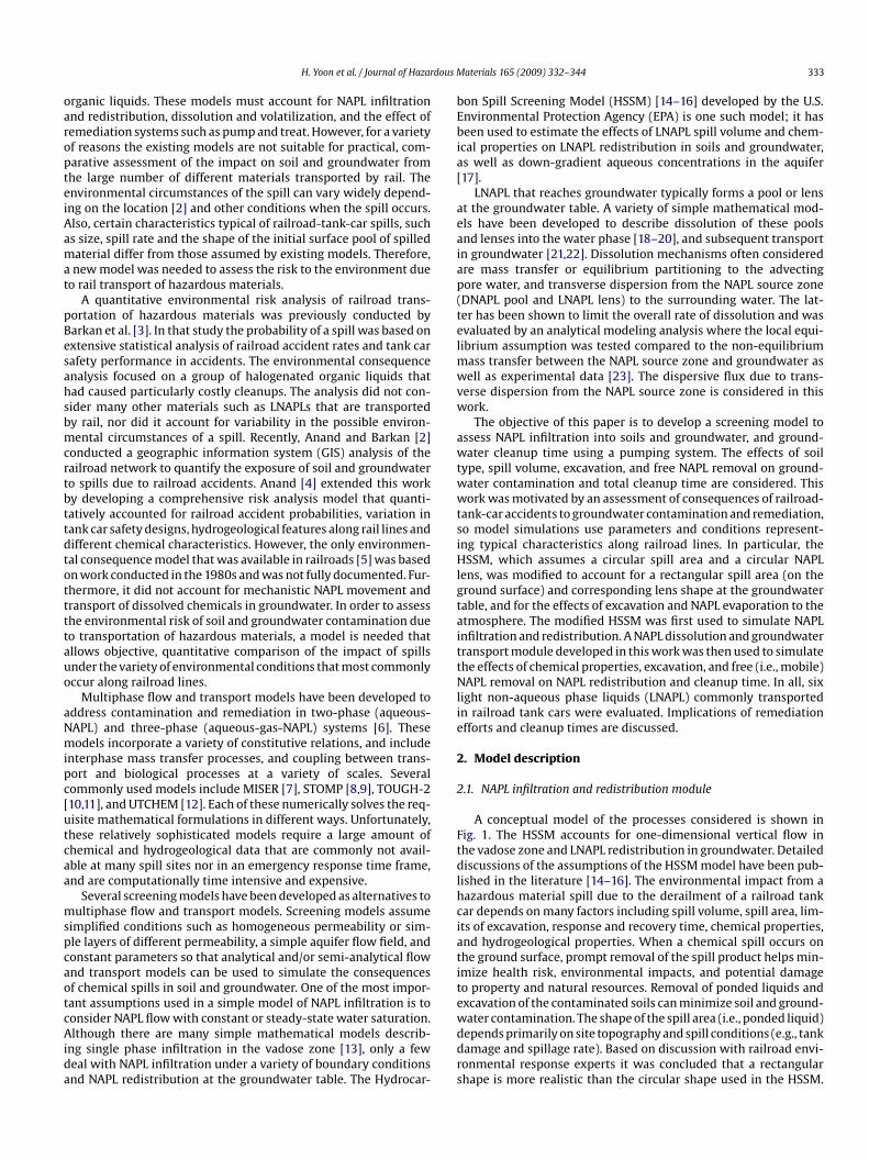
A conceptual model of the processes considered is shown inig. 1. The HSSM accounts for one-dimensional vertical flow inhe vadose zone and LNAPL redistribution in groundwater. Detailediscussions of the assumptions of the HSSM model have been pub-

ished in the literature [14–16]. The environmental impact from aazardous material spill due to the derailment of a railroad tankar depends on many factors including spill volume, spill area, lim-ts of excavation, response and recovery time, chemical properties,nd hydrogeological properties. When a chemical spill occurs onhe ground surface, prompt removal of the spill product helps min-mize health risk, environmental impacts, and potential damageo property and natural resources. Removal of ponded liquids andxcavation of the contaminated soils can minimize soil and ground-

ater contamination. The shape of the spill area (i.e., ponded liquid)epends primarily on site topography and spill conditions (e.g., tankamage and spillage rate). Based on discussion with railroad envi-onmental response experts it was concluded that a rectangularhape is more realistic than the circular shape used in the HSSM.

334 H. Yoon et al. / Journal of Hazardous Materials 165 (2009) 332–344

APL in

Tlas

laoarospmgfob

E

wi(ostac

k

wScc(a

(flLciam[

(irrz

k

wNrurowE

tLfsswsfcztltrapHttp

Fig. 1. Conceptual model of N

his is due to the proximity of drainage ditches adjacent to railroadines, where liquids often accumulate following a tank car spill. It islso not unusual to excavate and remove contaminated surface soil,o this factor also had to be accounted for in the modified HSSM.

A vadose zone flow and transport module (Kinematic Oily Pol-utant Transport, KOPT) in the HSSM was modified (KOPT-RAIL) toccount for the rectangular spill shape, excavation, and NAPL evap-ration to the atmosphere. The change of the spill shape does notffect vertical NAPL flow in the vadose zone, but does affect LNAPLedistribution in groundwater. After excavation, the top boundaryf the LNAPL plume in the vadose zone changes from the groundurface to the depth of excavation, assuming that LNAPL is com-letely removed by excavation to the depth of excavation. Theaximum depth of excavation is currently 6 m or the depth to the

roundwater table if less. The evaporation of a volatile liquid from aree-liquid surface to the atmosphere can affect the infiltration ratef liquids into soil. The evaporation rate of a liquid can be estimatedy Kawamura and Mackay [24]

= AkmCg (1)

here E is the evaporation rate (kg/s), A is the area of the evaporat-ng liquid pool (i.e., spill area), km is the mass transfer coefficientm/s), and Cg is the gas concentration of the liquid at the surfacef the pool (kg/m3), which can be computed using the vapor pres-ure and the ideal gas equation. An empirical equation for the massransfer coefficient during liquid evaporation developed by MacKaynd Matsugu [25] has been widely used, including for a NAPL spillase [26]:

m = cSc−2/3u7/9x−1/9 (2)

here c is a constant (0.0048) determined from experimental data,c is the Schmidt number, which is the ratio of the kinematic vis-osity of air (1.5 × 10−5 m2/s) to the molecular diffusivity of theompound in air (m2/s), u is the wind speed at a height of 10 mm/s), and x is the pool length in the wind direction (m). Eqs. (1)nd (2) were added to the KOPT module in the HSSM.

The constitutive saturation–pressure–relative permeabilityS–P–k) relation is a critical component of predictive multiphaseow models. In the residual NAPL formation theory developed byenhard et al. [27], the residual NAPL (i.e., NAPL held immobile by

apillary forces) saturation in the vadose zone is not constant, buts estimated as a function of saturation-path history. The Brooksnd Corey S–P model [28] with the Burdine relative permeabilityodel is used in the HSSM. In the new k–S–P relation updated by

27], the relative permeability for NAPL becomes zero as the free

att

[

filtration and redistribution.

i.e., mobile) NAPL saturation becomes zero. Since residual NAPL ismmobile, residual NAPL saturation does not contribute to NAPLelative permeability. This new NAPL relative permeability (krn)elation (Eq. (3)), including residual NAPL formation in the vadoseone [27], was added to the KOPT module as formulated below:

rn =(

Snf

1 − Swr

)2[(

Sw + Sn − Swr

1 − Swr

)((2+�)/�)

−(

Sw + Sgt − Swr

1 − Swr+ Snr

1 − Swr

)((2+�)/�)]

(3)

here Sn, Snf, and Snr are the total NAPL, free NAPL, and residualAPL saturations, respectively, Sw and Swr are the total water and

esidual water saturations, respectively, Sgt is the trapped air sat-ration, and � is the pore size distribution index. The maximumesidual NAPL saturation can be observed after complete drainagef NAPL from a soil initially saturated with NAPL at the residualater saturation. In groundwater, the residual NAPL saturation in

q. (3) was set to a constant value as used in the original HSSM.If a chemical spill is large and infiltrates into soil fast enough

o reach the groundwater table, and there is sufficient LNAPL head,NAPL will displace water downward and then spread laterally toorm a lens. The LNAPL distribution has two distinct regions afterpreading is complete (Fig. 1). The first is a zone of residual LNAPLaturation that marks the region where LNAPL displaced ground-ater downward before spreading outward to form a thin lens. The

econd is the thin LNAPL lens that eventually forms in the capillaryringe and on the groundwater table. The thickness of the lens wasalculated with the Dupuit assumptions, where the flow is hori-ontal and the gradient is independent of depth. Since the shape ofhe spill area is rectangular instead of circular, the spreading of theens is approximated by a rectangular shape in the x and y direc-ions (i.e., cross shape) as shown in Fig. 2. Based on discussion withailroad environmental response experts it was also concluded thatrectangular shape of the lens is practically realistic. For practicalurposes, the cross-shape of the lens predicted by the modifiedSSM was converted to a rectangular shape. The outer portions of

he lens in each direction (light gray parts in Fig. 2) were convertedo the same area of the rectangle in the converted lens (dark grayarts in Fig. 2). NAPL thicknesses over the light gray area were aver-

ged and the average NAPL thickness was distributed evenly overhe dark gray area. The converted lens was used for NAPL massransfer and dissolved plume development.

From the Dupuit equation and ho = hos at d = Ls and ho = 0 at d = Lt

29], the oil layer head (ho) at any distance (d) along the x and y

H. Yoon et al. / Journal of Hazardous Materials 165 (2009) 332–344 335

d

h

wotEotw

Q

wtstdcac(

V

fibtt

F

aa

m(afl(i.e., benzene) spilled in homogeneous coarse sand and silt consid-ered in this study, cumulative LNAPL volume across the capillaryfringe and the NAPL lens area for a 50% spill case (i.e., 50% of a tankcar volume) without excavation are shown in Figs. 3 and 4. The

Fig. 2. Schematic of lens spreading and conversion to a rectangular lens.

irections outside the rectangular source area (i.e., spill area) is

o(d) = hos

√Lt − d√

Lt − Ls/2(4)

here hos is the lens oil head beneath the spill area, Lt is the lengthf the oil lens from the spill center at time t, and Ls is the size ofhe source area in the x and y directions (i.e., Lx and Ly). As seen inq. (4), the lens oil head depends on hos and Lt. The rates of changef hos and Lt can be obtained by applying the continuity principleo the control volumes of the lens beneath the spill area and thehole lens, respectively, as

dhos

dt= 1

(LxLy)�oˇ(Qin − Qspreading − Qlosses) (5)

dLt

dt= Qin − Qlosses − (∂VTL/∂hos)(dhos/dt)

∂VTL/∂Lt(6)

spreading = −2LybosKodho

dx

∣∣∣x=Lx/2

− 2LxbosKodho

dy

∣∣∣x=Ly/2

(7)

here Qin is the volumetric NAPL flow rate into groundwater fromhe vadose zone, Qlosses are the mass losses of the lens due to dis-olution to groundwater, volatilization to the vadose zone, andhe formation of residual (or trapped) NAPL as the lens heightecreases, �o is an average effective volumetric NAPL content, ˇ is aonstant (=�w/(�w − �o)), �i is the density of phase i, bos is the aver-ge lens thickness in the source area, Ko is the effective hydrauliconductivity of the LNAPL at �o, and VTL is the total lens volumei.e., d = Lt). The lens volume, VL, as a function of distance (d) is

L(d) = LxLyˇhos + 2Lyˇ�ohos

(23

(Lt − Lx/2) − 23

(Lt − d)1.5√(Lt − Lx/2)

)

+ 2Lxˇ�ohos

(23

(Lt − Ly/2) − 23

(Lt − d)1.5√(Lt − Ly/2)

)(8)

Eqs. (5) and (6) are a system of ordinary differential equations

or the lens model and Eq. (8) is used to obtain the two derivativesn Eq. (6). The mass losses due to dissolution and volatilization cane computed using NAPL dissolution and volatilization module inhe next section. The details of the derivation and numerical solu-ion are provided in the HSSM Theory guide [16]. Eqs. (4)–(8) were

ig. 3. Comparison of the cumulative NAPL volume across the capillary fringe.

dded to the OILENS module in the HSSM (OILENS-RAIL) and allffected equations were also modified.

The modified HSSM was compared to the original HSSM and aultiphase simulator, Subsurface Transport Over Multiple Phases

STOMP) [8,9]. For STOMP simulations, both 1D vertical NAPL flownd 3D NAPL flow in the vadose zone were considered, and 3D NAPLow below the capillary fringe was considered. For a typical LNAPL

Fig. 4. Comparison of the lens area in (a) coarse sand and (b) silt.

3 dous M

osaastbotstcTtausamimm

2

aLacvuospecwsatp

asfNtais

J

s

q

wmcewvm

wep

k

w

zt

v

wctdtg

D

wtciE

C

wTflt

J

tCtpca

vfz

J

wtCfu

at

36 H. Yoon et al. / Journal of Hazar

riginal HSSM assumed a circular LNAPL pool shape at the groundurface whereas the modified HSSM and STOMP assume a rect-ngular shape. The comparison of the cumulative NAPL volumescross the capillary fringe in Fig. 3 showed that in two differentoils the NAPL volume in the modified HSSM was almost identicalo that in the original HSSM and within the range of STOMP resultsetween 3D and 1D NAPL flow in the vadose zone. The comparisonf the lens area in Fig. 4 showed that the modified HSSM predictedhe lens area well within the range of STOMP prediction in coarseand and 20% lower than that of STOMP prediction in silt. However,he original HSSM over-predicted and under-predict the lens area,ompared to STOMP results in coarse sand and silt, respectively.he main reason for the under-prediction of the modified HSSM inhe silt compared to the STOMP is that in the silt LNAPL can spreadbove the capillary fringe (i.e., unsaturated soil) in the STOMP sim-lation, while the modified HSSM considers NAPL flow only in theaturated zone. This difference decreased with increasing perme-bility because LNAPL can penetrate through the capillary fringeore easily with increasing permeability, resulting in less spread-

ng above the capillary fringe. This comparison indicates that theodified HSSM adequately captures the physics that govern LNAPLigration and lens formation.

.2. NAPL dissolution and volatilization module

Mass transfer from the LNAPL source zone (i.e., LNAPL lensnd residual LNAPL) is influenced by a variety of factors includingNAPL properties, the size of the LNAPL lens and residual region,nd the heterogeneity of porous media. The LNAPL lens in directontact with the water and gas phases undergoes dissolution andolatilization (Fig. 5). Residual LNAPL located below the LNAPL lensndergoes only dissolution. Rate-limited NAPL dissolution has beenbserved at high water velocities and low NAPL saturation. Manytudies have used a first-order mass transfer model to quantify thisrocess; experimental and numerical results are summarized in lit-rature [6,19,20,23,30]. Despite numerous investigations, it is notlear how to quantify NAPL dissolution rates in the field. In thisork, we modified the approach proposed by Falta [20] and con-

idered four components of NAPL mass flux from the source zone:dvective flux from groundwater flow, dispersive flux in the y direc-ion, dispersive flux in the z direction, and diffusive flux in the gashase toward the ground surface from the LNAPL lens.

The dissolved concentration within the LNAPL source zone isssumed to be in equilibrium with the NAPL phase; hence the dis-olved concentration is the aqueous solubility of the chemical. Thisollows from earlier work [23], where local equilibrium within aAPL source zone was found to adequately describe the concen-

ration driving force for dispersion under similar conditions. Thedvective flux through the LNAPL source (lens and residual), Jadv,s simply the product of the water specific discharge (q) and theolubility (Csol);

adv = qCsol (9)

The groundwater specific discharge varies as a function of wateraturation:

w = −krwk�wg

�wi (10)

here krw is the water relative permeability, k is the intrinsic per-eability of the soil, �w is the water density, g is the gravitational

onstant, �w is the water viscosity, and i is the hydraulic gradi-nt. The Brooks-Corey saturation–capillary pressure (S–P) modelith the Burdine relative permeability model (BCB model) and the

an-Genuchten S–P model with the Mualem relative permeabilityodel (VGM model) were used. Fluid entrapment and hysteresis

vtalr

aterials 165 (2009) 332–344

ere not considered due to complexity. The BCB model consid-rs a distinct nonwetting fluid entry pressure. The water relativeermeability, krw, is given by:

rw =(

Sw − Swr

1 − Swr

)((2+3�)/�)

(11)

here the water saturation, Sw, is simply (1 − Sn).The dissolved chemical concentration from the LNAPL source

one in the z direction is given by the steady-state dispersion equa-ion as developed by [31]:

∂C

∂x= Dt

∂2C

∂z2t

with C = Cin at x = 0, C = Csol at zt = 0,

C = 0 at zt → ∞ (12)

here v is the water pore velocity, Dt is the transverse dispersionoefficient, Cin is the influent dissolved chemical concentration, x ishe distance of the NAPL source zone along the groundwater flowirection, and zt are the transverse distance in the z direction fromhe NAPL source zone. The hydrodynamic dispersion coefficient isiven by:

t = Deff + v˛t (13)

here Deff is the effective diffusion coefficient and ˛t is theransverse dispersivity in the z direction. The effective diffusionoefficient is the product of the tortuosity, which is simply porosityn this study, and the aqueous diffusion coefficient. The solution toq. (12) is

(Lx, zt) = Cin + (Csol − Cin)erfc

(zt

2√

DtLx/v

)(14)

here Lx is the horizontal distance along the LNAPL source zone.he same approach is considered in the y direction. The total massux from each direction can be obtained by integrating the concen-ration with respect to z and y:

disp = (Csat − Cin)�√

4DtvLx/� (15)

The NAPL dissolution processes implemented in this study wereested against a three-dimensional NAPL dissolution data set [32].omparison of simulated and experimental average effluent flux athe end of the 3D sandbox showed that among four cases, averageercent error in the two best cases was less than 5% and in onease was less than 25%, and total NAPL removal time was predictedccurately (i.e., within 6%) [32].

LNAPL in direct contact with the gas phase is depleted by NAPLolatilization. NAPL volatilization is described using Fick’s First Lawor steady-state vapor transport toward the ground surface with aero concentration boundary:

v = −DveffdC

dz= Dveff

Cvsat

Zdepth(16)

here Jv is the vapor diffusive flux from the top of the LNAPL tohe ground surface, Dveff is the effective vapor diffusion coefficient,vsat is the saturated gas concentration, and Zdepth is the distancerom the top of the LNAPL to the ground surface. Dveff is computedsing the Millington and Quirk [33] equation.

In this work, a simplified 3D source geometry was used toccommodate the variety of LNAPL distributions that result fromhe modified HSSM. The continuous LNAPL distribution was con-

erted into a discrete 3D geometry by volumetric averaging. Thewo distinct NAPL source zones (i.e., lens and residual zones) wereveraged differently. First, the LNAPL lens was averaged into twoayers, in which NAPL saturations were volumetric average satu-ations above and below the groundwater table. The LNAPL lens

H. Yoon et al. / Journal of Hazardous M

FSd

tttdLcNbcag

attadg(gbgilfftdl

2

o[a(tidtdttodcNtflrrw3TWimipw(lc

2

Nrs

FP

ig. 5. Schematic of four different NAPL dissolution and volatilization processes.chematic shows half of the LNAPL source zone by symmetry along the main flowirection.

hickness decreased with increasing distance from the center ofhe LNAPL source, resulting in varying LNAPL saturation over dis-ance. The scale of a grid block was 0.5 m × 0.5 m in the horizontalirection and varied in the vertical direction depending upon theNAPL lens thickness. Second, the length of residual NAPL was cal-ulated based upon a threshold saturation below which no residualAPL exists. Since in most cases the residual NAPL zone was locatedelow the center of the NAPL source, the residual NAPL zone wasonsidered as a rectangular shape (Fig. 1). The vertical grid in therea of residual NAPL (i.e., below the LNAPL lens) was 0.02 m. Therid spacing can be easily adjusted.

Semi-analytical solutions that update the size of the source areand NAPL saturation over time are used to reduce computationalime as follows. First, NAPL dissolution due to the advecting waterhrough a grid block occurs within the first grid block upgradientlong the groundwater flow direction, but there is no net NAPLissolution by advection through the remaining grid blocks down-radient. Second, the dispersive flux in the z and y directions (Eq.15)) is updated in two regions: the dispersive flux from the firstrid block upgradient is used to revise the NAPL saturation in thelock. The NAPL saturations in the rest of the NAPL blocks down-radient are updated based on the average dispersive flux, whichs the difference between the total dispersive flux along the entireength of the LNAPL source zone and the average dispersive fluxrom the upgradient grid block(s). As a result, NAPL is removed first

rom the upgradient block of the source zone advectively, and fromhe bottom and the side of the source zone dispersively. Finally, theiffusive flux (Eq. (16)) due to NAPL volatilization from the LNAPL

ens is computed (Fig. 5).

lopdt

ig. 6. Plan view of pumping systems for NAPL removal and capturing dissolved plume. Coarameters for coarse sand in Table 2 were used.

aterials 165 (2009) 332–344 337

.3. Contaminant transport module

The end of the LNAPL source zone serves as the source planef the dissolved chemical transport zone (Fig. 1). The Domenico34] solution with Martin-Hayden and Robbins [35] improvementsnd first-order biodegradation implemented in BIOCHLOR [36]referred in this work as the “modified Domenico model”) was usedo calculate downgradient dissolved contaminant concentrations;t considers advection, dispersion, linear sorption, an exponentiallyecaying source boundary condition, and first-order biodegrada-ion in the aqueous phase. The original Domenico model waserived for a single planar source of constant concentration. Inhis work, the Domenico model was modified by superimposinghe Domenico solution over multiple source areas as a functionf time (Fig. 6). As the NAPL source zone configuration changedue to dissolution and volatilization, the transient solution for theoncentrations over multiple source areas was computed using theAPL dissolution and volatilization module. The concentrations at

he source planes were computed by considering the total massux due to advection and dispersion divided by the average flowate. The number of source planes can be easily adjusted. The accu-acy of the modified Domenico solution implemented in this workas compared against the exact semi-analytical solution for theD transport problem using a program PATCHI in Wexler [37].he results in this work showed good agreement with those fromexler [37] as shown in Fig. 6. As described in considerable detail

n several recent reviews [38–40], the accuracy of the Domenicoodel depends mostly upon the value of longitudinal dispersiv-

ty and the position of the advective front of the plume. Since theroblems presented in this study consider relatively short ground-ater plumes because cleanup begins quickly after a spill occurs

e.g., 30 days), the modified Domenico model can be used becauseongitudinal dispersivity is small due to the short distance of theontamination plume.

.4. Pumping module

Two different pumping systems were used to remove theAPL source zone and capture contaminated groundwater plume,

espectively (Fig. 6). For NAPL source zone removal, the pumpingystem is located downgradient from the NAPL source zone. The

ocation of pumping wells is determined by minimizing the numberf pumping wells and capturing the entire NAPL source zone. Theumping system for capturing the groundwater plume is locatedowngradient from that for NAPL source zone removal. Hence,wo pumping systems are separated by a water divide. For both

mparison of the modified Domenico model and Wexler (1992)’s solution is shown.

338 H. Yoon et al. / Journal of Hazardous Materials 165 (2009) 332–344

Table 1Chemical properties used in simulationsa.

Chemicals Density (kg/L) Viscosity (cp) NAPL water interfacialtension (dyne/cm)

Water surfacetension (dyne/cm)

Solubility (mg/L) Vapor Pressure (atm) Diffusion coefficientin gas (cm2/s)

Acrylonitrile 0.801 0.35 10.381 50.51 7.45E+04 0.072 0.106Benzene 0.877 0.604 35 60.6 1.78E+03 0.0846 0.09Cyclohexane 0.774 0.894 50.0 72.0 5.50E+01 0.0803 0.074MTBE 0.735 0.333 10.52 30.52 5.00E+04 0.217 0.075Styrene 0.902 0.695 32.5 62.5 3.10E+02 0.0059 0.071Vinyl acetate 0.926 0.421 30.0 54.0 2.30E+04 0.11 0.085

D APL-w[ 52]. Vp wate

15 ◦C.

piataotaiiio

swboiFtHoztiSzpaNiEn[

V

V

v

wywtat

b

t

wi

3

tTsTib3sSWs

livpabout 45,000 to over 115,000 L. The distribution of spill amountsfrom tank cars in mainline accidents can be considered in termsof percentage tank capacity lost in a release accident [47]. For thisstudy we used the percentage categories, 0–5%, 5–20%, 20–80%,and 80–100% and assumed the arithmetic mean quantity spilled for

Table 2Soil properties used in simulations.

Physical properties Coarse sand Fine sand Silt

Hydraulic conductivity (m/d) 50 7 1Hydraulic gradient 0.006 0.006 0.006Pore size distribution index 1.5 0.5 0.5Air entry pressure (m) 0.15 0.3 0.5Residual water saturation 0.048 0.1 0.2Maximum residual NAPL

saturation in the vadose zone0.03 0.05 0.10

Residual NAPL saturation ingroundwater

0.1 0.1 0.1

Lens NAPL saturation 0.35 0.35 0.35Effective porosity 0.42 0.33 0.33Horizontal transverse dispersivity 0.05 0.05 0.05

ensity and viscosity were from the Hazardous Substances Data Bank (HSDB) [50]. N51] and HSDB [50]. Solubility and diffusion coefficient in gas were from U.S. EPA [roperties of butyronitrile in Demond and Lindner [51]. 2From Hickel et al. [54] anda All data were in the range of 20–25 ◦C except for saturated gas concentration at

umping systems, the domain is assumed to be homogeneous,sotropic, and with constant groundwater flow. For an unconfinedquifer with the fully penetrated pumping well, the Dupuit assump-ion (i.e., vertical gradients are negligible) is commonly used innalytical groundwater modeling [29,41,42]. Recently, the effectf the drawdown in an unconfined aquifer (i.e., variation of waterable) on the travel time to a pumping well was compared to that inconfined aquifer [42]. For an aquifer thickness of 10 m considered

n this study and a drawdown of 2 m at the well, the error for ignor-ng the effect of the drawdown was less than 10% [42]. As indicatedn [42], the effect of the vertical flow needs to be tested if the ratiof the drawdown to the aquifer thickness is greater than 0.5.

The number of pumping wells for two pumping systems waseparately computed. The number of NAPL source zone removalells was computed by dividing the width of the NAPL source zone

y the minimum width of a single well capture zone. The numberf wells for capturing the plume was computed similarly by divid-ng the plume width by the width of a single well capture zone.or low solubility chemicals, the NAPL removal time is expectedo be much longer than the time required to capture the plume.ence, only the pumping system for NAPL source zone removal isperated after all the dissolved plume is captured. For NAPL sourceone removal, no NAPL flow is assumed. If NAPL flow is expectedo be significant, free-product removal can be used before pump-ng. The effect of free NAPL removal on cleanup time was tested inection 4. It was assumed that all remaining NAPL in the vadoseone was removed by soil excavation or soil vapor extraction whenumping begins. Hence, NAPL in the vadose zone is not consideredlong-term source of groundwater contamination after pumping.APL removal processes during pumping are the same as described

n the previous section, only the groundwater flow velocity (v) inqs. (13)–(15) is different. The groundwater flow velocity compo-ents Vx and Vy in the x and y directions, respectively, are given by41,43]:

x = q

�+ Qwx

2��B(x2 + y2)(17)

y = Qwy

2��B(x2 + y2)(18)

=√

V2x + V2

y (19)

here Qw is the rate of pumping, B is the aquifer thickness, x and

are the distances to the pumping well. For capturing the ground-ater plume, a model using the concept of arrival distribution

ime [44] was chosen for this study. The details of the method arevailable in Kinzelbach [45]. The time required to capture the con-aminant plume is the travel time of the contaminant from the outer

V

LT

ater interfacial tension and water surface tension were from Demond and Lindnerapor pressure was from Ohe [53] and HSDB [50]. 1These data are based upon ther surface tension is computed by assuming a zero spreading coefficient.

oundary of the plume to the pumping well and is calculated as [45]

plume = �QwR

2�v2B

(L

2�vB

Qw− ln

(L

2�vB

Qw+ 1))

(20)

here R is the retardation factor, and L is the distance to the pump-ng well.

. Example problems

Six LNAPLs frequently shipped in railroad tank cars were usedo illustrate the effects of chemical properties on cleanup (Table 1).he hydrogeological properties and transport parameters of threeoil types, coarse sand, fine sand, and silt, were considered (Table 2).he modeling domain was assumed to be homogeneous andsotropic and all parameters used in this study were assumed toe constant over time. Four depths to groundwater, 3, 6, 15, and0 m, were used in the simulations. These depths were chosen topan the most common depths identified from a U.S. Geologicalurvey (USGS) dataset of the groundwater depth in the U.S. [46].ater saturation in the vadose zone is assumed at residual water

aturation.The spill volume in a tank car accident can vary from a few

iters to the entire tank car contents. The maximum amount spilleds also affected by the volumetric capacity of the tank car, whicharies depending on the density of product it is intended to trans-ort. The capacity of most North American tank cars ranges from

in the NAPL source (m)ertical transverse dispersivity inthe NAPL source (m)

0.025 0.025 0.025

ongitudinal dispersivity (m) 1 1 1ransverse dispersivity (m) 0.1 0.1 0.1

H. Yoon et al. / Journal of Hazardous Materials 165 (2009) 332–344 339

Table 3Input parameters used in simulations.

Condition Value assumed

Size of a tank car (m3) 99.30Spill duration (hrs) 12Maximum depth of excavation (m) 6Excavation time (days) 4Remediation time (days) 30Aquifer thickness (m) 10

Soil-type-specific conditions Coarse sand Fine sand Silt

Spill length (m), Lx 1.5 3.0 4.5

Spillwidth(m),Ly

2.5% spill 3 3 4.512.5% spill 6 6 1250% spill 16.7 16.7 30.590% spill 30 30 61

P

Fw

escttrodtwr

dwttsmeNtSstpatnttic

4

4

cNcwtti

Fig. 7. NAPL amounts across the capillary fringe in (a) coarse sand, (b) fine sand,and (c) silt. The percentage represents the percentage spill of a tank car volume(S(

dwfi

sriNieTpeldr1iNslv5v

umping rate (m3/d) 200 200 20

or 50% and 90% spill cases, infiltration rate (=spill volume/spill area/spill duration)as almost the same.

ach respective category as follows, 2.5%, 12.5%, 50%, and 90%. In thistudy we assumed a tank volume of 99.3 m3, a size typical of tankars used for many NAPLs. A variety of other assumptions also hado be made for purposes of comparison (Table 3). It was assumedhat all spill volumes, except for the fraction of NAPL that evapo-ates, infiltrate into the soil. The spill width was determined basedn expert opinion and actual accident records [4]. The spill area wasetermined based on the spill width and volume and run-off overhe ground surface was not considered. Groundwater remediationas assumed to begin 30 days after the spill based on anticipated

esponse times for cleanup by railroad personnel.Unless otherwise stated, excavation was assumed complete four

ays after the spill occurred, and the maximum excavation depthas six m. We also compared the effect of no excavation and excava-

ion after only two days. The effect of free NAPL recovery on cleanupime for low solubility chemicals was also investigated. In thistudy, no module was developed for free NAPL recovery. Instead, allobile NAPL was removed before pumping in order to evaluate the

ffect on cleanup time; hence remaining NAPL was set to a residualAPL saturation. The importance of free NAPL recovery highlights

he importance of using free-product recovery at real field sites.ince remediation was assumed to start within a month, for lowolubility chemicals the contaminant plume did not move far fromhe NAPL source zone and thus a few pumping wells can capture thelume down gradient. For high solubility chemicals (>10,000 mg/L)pumping rate of 20 m3/d was used since preliminary tests showed

his pumping rate is enough to capture the contaminant plume. Theumber of pumping wells and pumping time required to removehe contaminant plume and NAPL source zone were computed. Forhe purposes of this paper, groundwater cleanup time by the pump-ng well system was computed for the NAPL source zone and theontaminant plume.

. Results and discussion

.1. NAPL volume in groundwater

The NAPL volume that reached groundwater for the six chemi-als was calculated at 30 days after the spill occurred (Fig. 7). TheAPL saturation was close to one near the ground surface in most

ases. A sharp front of constant NAPL saturation migrated down-ard until the NAPL pool at the ground surface was depleted. After

his, the NAPL saturation decreased as the NAPL front continuedo migrate downward, and residual NAPL was left behind trappedn the pore space. The NAPL relative permeability decreased with

wflia

99.1 m3). The end of each bar represents NAPL volume across the capillary fringe.ix chemicals are acrylonitrile (Acryl), vinyl acetate (Vinyl), MTBE (MTB), benzeneBenz), styrene (Styre), and cyclohexane (Cyclo).

ecreasing NAPL saturation, resulting in slower NAPL migrationith time. If the spilled NAPL volume and migration rate were suf-ciently large, a portion of the spilled NAPL reached groundwater.

The six chemicals considered in this study have vapor pres-ures ranging from 0.0059 to 0.217 atm, and density to viscosityatios ranging from 0.8 to 2.3 kg/L/cP. The chemicals are presentedn Fig. 7 from left to right in order of decreasing vapor pressure.APL amounts that reached groundwater increase with decreas-

ng vapor pressure for groundwater depths up to six m with thexception of vinyl acetate due to its high density to viscosity ratio.he total amount of NAPL that evaporates to the atmosphere isroportional to the spill area (Eq. (1)). The more NAPL mass thatvaporates, the less NAPL mass that infiltrates into soils, particu-arly, in silt because it has a larger spill area than the other soilsue to its lower permeability (Table 2). For example, NAPL evapo-ation into the atmosphere for MTBE accounted for approximately2%, 24%, and 48% of the total spill amount for a 90% spill casen the coarse sand, fine sand, and silt, respectively. The effect ofAPL evaporation for benzene, acrylonitrile, and styrene was notignificant due to the short period of the NAPL spill (12 h) and theower vapor pressures of these compounds (Table 1). Acrylonitrile,inyl acetate, and MTBE have ratios of density to viscosity within%; NAPL amounts that reached groundwater were very similar forinyl acetate and acrylonitrile at all depths, but the NAPL amountas smaller for MTBE, mainly due to its high vapor pressure. Except

or MTBE with the highest vapor pressure and for styrene with theowest vapor pressure, the NAPL amount that reached groundwaterncreased with increasing values of the density to viscosity ratio forll groundwater depths and in all soils (Fig. 7).

340 H. Yoon et al. / Journal of Hazardous M

Ffi

(tnmFdpNfdict

4

4

fsicM(i

Nscc

dsicswpafatctgr

aarucmdltt2

ticdiopihrN

4

tftietctcwNltcoarse sand and silt. These results imply that for low permeability

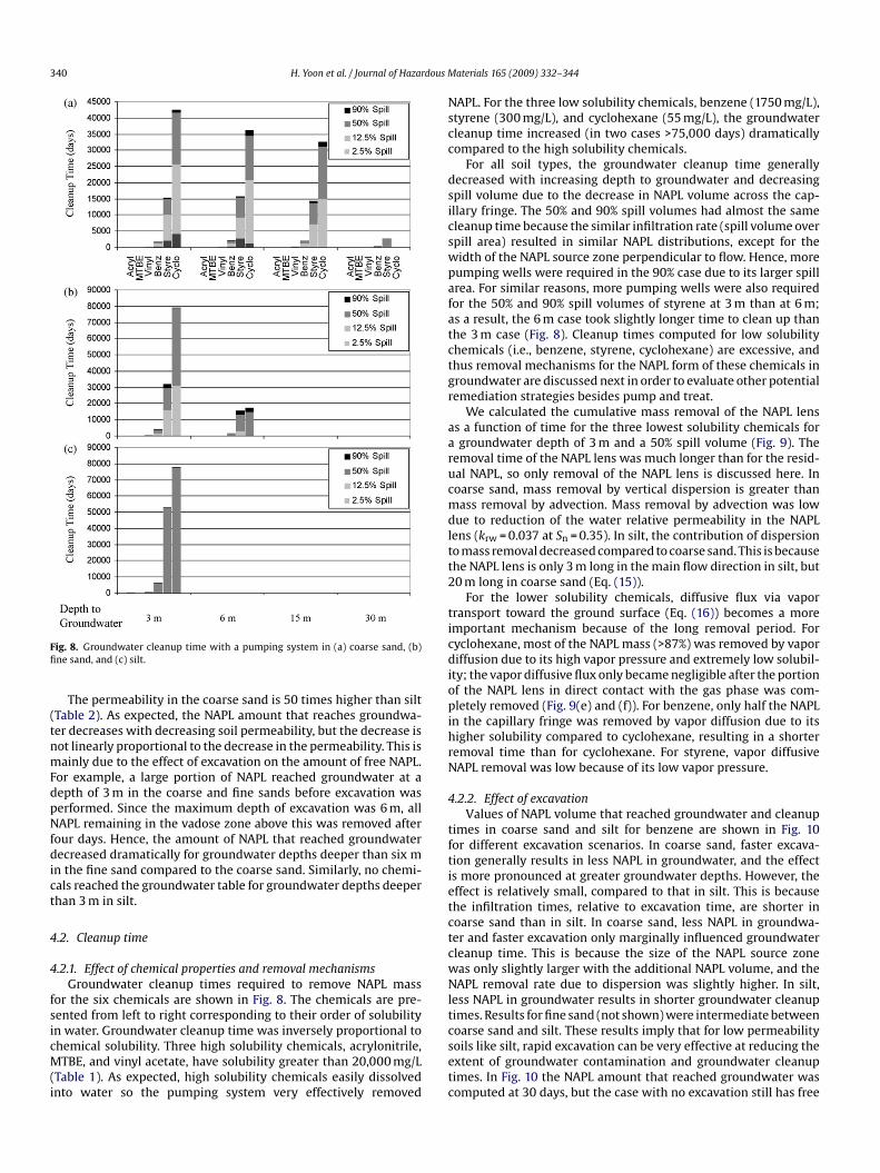
ig. 8. Groundwater cleanup time with a pumping system in (a) coarse sand, (b)ne sand, and (c) silt.

The permeability in the coarse sand is 50 times higher than siltTable 2). As expected, the NAPL amount that reaches groundwa-er decreases with decreasing soil permeability, but the decrease isot linearly proportional to the decrease in the permeability. This isainly due to the effect of excavation on the amount of free NAPL.

or example, a large portion of NAPL reached groundwater at aepth of 3 m in the coarse and fine sands before excavation waserformed. Since the maximum depth of excavation was 6 m, allAPL remaining in the vadose zone above this was removed after

our days. Hence, the amount of NAPL that reached groundwaterecreased dramatically for groundwater depths deeper than six m

n the fine sand compared to the coarse sand. Similarly, no chemi-als reached the groundwater table for groundwater depths deeperhan 3 m in silt.

.2. Cleanup time

.2.1. Effect of chemical properties and removal mechanismsGroundwater cleanup times required to remove NAPL mass

or the six chemicals are shown in Fig. 8. The chemicals are pre-ented from left to right corresponding to their order of solubilityn water. Groundwater cleanup time was inversely proportional to

hemical solubility. Three high solubility chemicals, acrylonitrile,TBE, and vinyl acetate, have solubility greater than 20,000 mg/L

Table 1). As expected, high solubility chemicals easily dissolvednto water so the pumping system very effectively removed

setc

aterials 165 (2009) 332–344

APL. For the three low solubility chemicals, benzene (1750 mg/L),tyrene (300 mg/L), and cyclohexane (55 mg/L), the groundwaterleanup time increased (in two cases >75,000 days) dramaticallyompared to the high solubility chemicals.

For all soil types, the groundwater cleanup time generallyecreased with increasing depth to groundwater and decreasingpill volume due to the decrease in NAPL volume across the cap-llary fringe. The 50% and 90% spill volumes had almost the sameleanup time because the similar infiltration rate (spill volume overpill area) resulted in similar NAPL distributions, except for theidth of the NAPL source zone perpendicular to flow. Hence, moreumping wells were required in the 90% case due to its larger spillrea. For similar reasons, more pumping wells were also requiredor the 50% and 90% spill volumes of styrene at 3 m than at 6 m;s a result, the 6 m case took slightly longer time to clean up thanhe 3 m case (Fig. 8). Cleanup times computed for low solubilityhemicals (i.e., benzene, styrene, cyclohexane) are excessive, andhus removal mechanisms for the NAPL form of these chemicals inroundwater are discussed next in order to evaluate other potentialemediation strategies besides pump and treat.

We calculated the cumulative mass removal of the NAPL lenss a function of time for the three lowest solubility chemicals forgroundwater depth of 3 m and a 50% spill volume (Fig. 9). The

emoval time of the NAPL lens was much longer than for the resid-al NAPL, so only removal of the NAPL lens is discussed here. Inoarse sand, mass removal by vertical dispersion is greater thanass removal by advection. Mass removal by advection was low

ue to reduction of the water relative permeability in the NAPLens (krw = 0.037 at Sn = 0.35). In silt, the contribution of dispersiono mass removal decreased compared to coarse sand. This is becausehe NAPL lens is only 3 m long in the main flow direction in silt, but0 m long in coarse sand (Eq. (15)).

For the lower solubility chemicals, diffusive flux via vaporransport toward the ground surface (Eq. (16)) becomes a moremportant mechanism because of the long removal period. Foryclohexane, most of the NAPL mass (>87%) was removed by vaporiffusion due to its high vapor pressure and extremely low solubil-

ty; the vapor diffusive flux only became negligible after the portionf the NAPL lens in direct contact with the gas phase was com-letely removed (Fig. 9(e) and (f)). For benzene, only half the NAPL

n the capillary fringe was removed by vapor diffusion due to itsigher solubility compared to cyclohexane, resulting in a shorteremoval time than for cyclohexane. For styrene, vapor diffusiveAPL removal was low because of its low vapor pressure.

.2.2. Effect of excavationValues of NAPL volume that reached groundwater and cleanup

imes in coarse sand and silt for benzene are shown in Fig. 10or different excavation scenarios. In coarse sand, faster excava-ion generally results in less NAPL in groundwater, and the effects more pronounced at greater groundwater depths. However, theffect is relatively small, compared to that in silt. This is becausehe infiltration times, relative to excavation time, are shorter inoarse sand than in silt. In coarse sand, less NAPL in groundwa-er and faster excavation only marginally influenced groundwaterleanup time. This is because the size of the NAPL source zoneas only slightly larger with the additional NAPL volume, and theAPL removal rate due to dispersion was slightly higher. In silt,

ess NAPL in groundwater results in shorter groundwater cleanupimes. Results for fine sand (not shown) were intermediate between

oils like silt, rapid excavation can be very effective at reducing thextent of groundwater contamination and groundwater cleanupimes. In Fig. 10 the NAPL amount that reached groundwater wasomputed at 30 days, but the case with no excavation still has free

H. Yoon et al. / Journal of Hazardous Materials 165 (2009) 332–344 341

F olatiliza 50% of

Nc

4

aWlpfdue0sr

actbs

dttsi

ig. 9. Cumulative mass removal of the NAPL lens by NAPL dissolution and NAPL vnd (e and f) cyclohexane. The depth to groundwater is 3 m and the spill volume is

APL in the vadose zone, which has the potential to cause furtherontamination.

.2.3. Effect of free NAPL removalGroundwater cleanup times for benzene, styrene, and cyclohex-

ne in the three soils with free NAPL removal are shown in Fig. 11.hen free NAPL removal is considered, NAPL saturation in the NAPL

ens is reduced to a residual NAPL saturation of 0.1 as describedreviously. For all cases, cleanup times decrease significantly by a

actor of 2–7 when free NAPL removal is considered. This is mainlyue to the increase in the water relative permeability as NAPL sat-

rations decrease, and the decrease in the total NAPL mass. Forxample, the water relative permeability increased from 0.037 to.6 as the NAPL saturation decreased from 0.35 to 0.1 in coarseand. Comparison of cleanup times with and without free NAPLemoval (Figs. 8 and 11) reveals that the trends in cleanup times as

dfgrt

ation in coarse sand (left) and silt (right) for (a and b) benzene, (c and d) styrene,a tank car.

function of depths to groundwater did not change, but the scale ofleanup times changed for all three chemicals. This is attributed tohe assumption that free NAPL removal reduced NAPL saturation,ut did not change the size of the NAPL source zone, resulting inimilar dispersive fluxes and faster NAPL dissolution by advection.

For 50% and 90% spill cases, cleanup time increased withecreasing soil permeability at the 3 m groundwater depth. In con-rast, for 12.5% spill cases, cleanup time did not follow this trend athe same depth. This is because NAPL volume in groundwater in theilt is much smaller than NAPL volume in the sand (Fig. 7), result-ng in a longer cleanup time in the sand. Hence, cleanup times in

ifferent soils are strongly affected by chemical solubility and dif-usion coefficient values in the gas phase as well as NAPL volume inroundwater. In addition, the scale of cleanup time with free NAPLemoval for styrene and cyclohexane is still very high because ofheir low solubilities.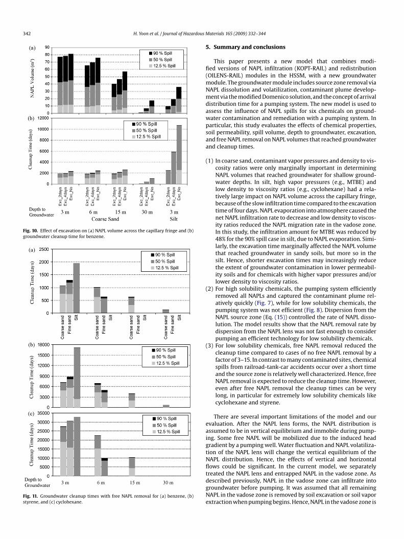

342 H. Yoon et al. / Journal of Hazardous M

Fig. 10. Effect of excavation on (a) NAPL volume across the capillary fringe and (b)groundwater cleanup time for benzene.

Fig. 11. Groundwater cleanup times with free NAPL removal for (a) benzene, (b)styrene, and (c) cyclohexane.

5

fi(mNmdawpsaa

(

(

(

eaigtNfltdgNe

aterials 165 (2009) 332–344

. Summary and conclusions

This paper presents a new model that combines modi-ed versions of NAPL infiltration (KOPT-RAIL) and redistributionOILENS-RAIL) modules in the HSSM, with a new groundwater

odule. The groundwater module includes source zone removal viaAPL dissolution and volatilization, contaminant plume develop-ent via the modified Domenico solution, and the concept of arrival

istribution time for a pumping system. The new model is used tossess the influence of NAPL spills for six chemicals on ground-ater contamination and remediation with a pumping system. Inarticular, this study evaluates the effects of chemical properties,oil permeability, spill volume, depth to groundwater, excavation,nd free NAPL removal on NAPL volumes that reached groundwaternd cleanup times.

1) In coarse sand, contaminant vapor pressures and density to vis-cosity ratios were only marginally important in determiningNAPL volumes that reached groundwater for shallow ground-water depths. In silt, high vapor pressures (e.g., MTBE) andlow density to viscosity ratios (e.g., cyclohexane) had a rela-tively large impact on NAPL volume across the capillary fringe,because of the slow infiltration time compared to the excavationtime of four days. NAPL evaporation into atmosphere caused thenet NAPL infiltration rate to decrease and low density to viscos-ity ratios reduced the NAPL migration rate in the vadose zone.In this study, the infiltration amount for MTBE was reduced by48% for the 90% spill case in silt, due to NAPL evaporation. Simi-larly, the excavation time marginally affected the NAPL volumethat reached groundwater in sandy soils, but more so in thesilt. Hence, shorter excavation times may increasingly reducethe extent of groundwater contamination in lower permeabil-ity soils and for chemicals with higher vapor pressures and/orlower density to viscosity ratios.

2) For high solubility chemicals, the pumping system efficientlyremoved all NAPLs and captured the contaminant plume rel-atively quickly (Fig. 7), while for low solubility chemicals, thepumping system was not efficient (Fig. 8). Dispersion from theNAPL source zone (Eq. (15)) controlled the rate of NAPL disso-lution. The model results show that the NAPL removal rate bydispersion from the NAPL lens was not fast enough to considerpumping an efficient technology for low solubility chemicals.

3) For low solubility chemicals, free NAPL removal reduced thecleanup time compared to cases of no free NAPL removal by afactor of 3–15. In contrast to many contaminated sites, chemicalspills from railroad-tank-car accidents occur over a short timeand the source zone is relatively well characterized. Hence, freeNAPL removal is expected to reduce the cleanup time. However,even after free NAPL removal the cleanup times can be verylong, in particular for extremely low solubility chemicals likecyclohexane and styrene.

There are several important limitations of the model and ourvaluation. After the NAPL lens forms, the NAPL distribution isssumed to be in vertical equilibrium and immobile during pump-ng. Some free NAPL will be mobilized due to the induced headradient by a pumping well. Water fluctuation and NAPL volatiliza-ion of the NAPL lens will change the vertical equilibrium of theAPL distribution. Hence, the effects of vertical and horizontalows could be significant. In the current model, we separately

reated the NAPL lens and entrapped NAPL in the vadose zone. Asescribed previously, NAPL in the vadose zone can infiltrate intoroundwater before pumping. It was assumed that all remainingAPL in the vadose zone is removed by soil excavation or soil vaporxtraction when pumping begins. Hence, NAPL in the vadose zone is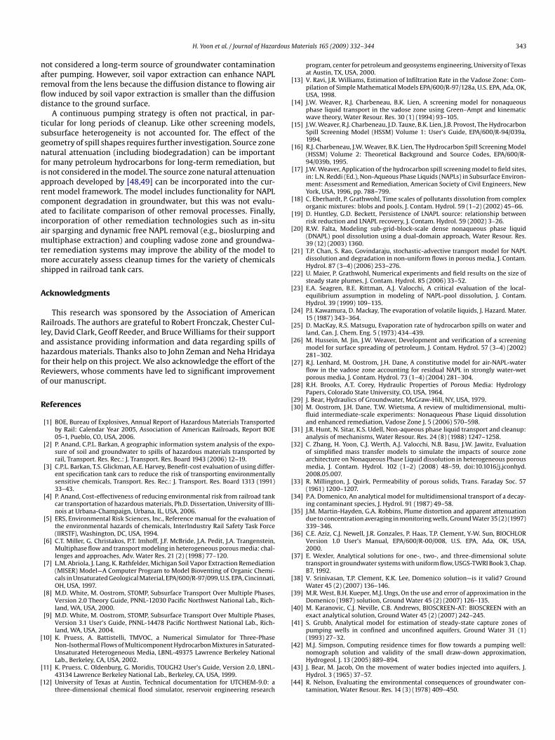

dous M

narfld

tsgnfiarcaiamtms

A

RlahfRo

R

[

[

[

[

[

[

[

[

[

[

[

[

[

[

[

[

[

[

[

[[

[

[

[

[

[

[

[

[

[

[

[

[

H. Yoon et al. / Journal of Hazar

ot considered a long-term source of groundwater contaminationfter pumping. However, soil vapor extraction can enhance NAPLemoval from the lens because the diffusion distance to flowing airow induced by soil vapor extraction is smaller than the diffusionistance to the ground surface.

A continuous pumping strategy is often not practical, in par-icular for long periods of cleanup. Like other screening models,ubsurface heterogeneity is not accounted for. The effect of theeometry of spill shapes requires further investigation. Source zoneatural attenuation (including biodegradation) can be important

or many petroleum hydrocarbons for long-term remediation, buts not considered in the model. The source zone natural attenuationpproach developed by [48,49] can be incorporated into the cur-ent model framework. The model includes functionality for NAPLomponent degradation in groundwater, but this was not evalu-ted to facilitate comparison of other removal processes. Finally,ncorporation of other remediation technologies such as in-situir sparging and dynamic free NAPL removal (e.g., bioslurping andultiphase extraction) and coupling vadose zone and groundwa-

er remediation systems may improve the ability of the model toore accurately assess cleanup times for the variety of chemicals

hipped in railroad tank cars.

cknowledgments

This research was sponsored by the Association of Americanailroads. The authors are grateful to Robert Fronczak, Chester Cul-

ey, David Clark, Geoff Reeder, and Bruce Williams for their supportnd assistance providing information and data regarding spills ofazardous materials. Thanks also to John Zeman and Neha Hridaya

or their help on this project. We also acknowledge the effort of theeviewers, whose comments have led to significant improvementf our manuscript.

eferences

[1] BOE, Bureau of Explosives, Annual Report of Hazardous Materials Transportedby Rail: Calendar Year 2005, Association of American Railroads, Report BOE05-1, Pueblo, CO, USA, 2006.

[2] P. Anand, C.P.L. Barkan, A geographic information system analysis of the expo-sure of soil and groundwater to spills of hazardous materials transported byrail, Transport. Res. Rec.: J. Transport. Res. Board 1943 (2006) 12–19.

[3] C.P.L. Barkan, T.S. Glickman, A.E. Harvey, Benefit-cost evaluation of using differ-ent specification tank cars to reduce the risk of transporting environmentallysensitive chemicals, Transport. Res. Rec.: J. Transport. Res. Board 1313 (1991)33–43.

[4] P. Anand, Cost-effectiveness of reducing environmental risk from railroad tankcar transportation of hazardous materials, Ph.D. Dissertation, University of Illi-nois at Urbana-Champaign, Urbana, IL, USA, 2006.

[5] ERS, Environmental Risk Sciences, Inc., Reference manual for the evaluation ofthe environmental hazards of chemicals, InterIndustry Rail Safety Task Force(IIRSTF), Washington, DC, USA, 1994.

[6] C.T. Miller, G. Christakos, P.T. Imhoff, J.F. McBride, J.A. Pedit, J.A. Trangenstein,Multiphase flow and transport modeling in heterogeneous porous media: chal-lenges and approaches, Adv. Water Res. 21 (2) (1998) 77–120.

[7] L.M. Abriola, J. Lang, K. Rathfelder, Michigan Soil Vapor Extraction Remediation(MISER) Model—A Computer Program to Model Bioventing of Organic Chemi-cals in Unsaturated Geological Material, EPA/600/R-97/099, U.S. EPA, Cincinnati,OH, USA, 1997.

[8] M.D. White, M. Oostrom, STOMP, Subsurface Transport Over Multiple Phases,Version 2.0 Theory Guide, PNNL-12030 Pacific Northwest National Lab., Rich-land, WA, USA, 2000.

[9] M.D. White, M. Oostrom, STOMP, Subsurface Transport Over Multiple Phases,Version 3.1 User’s Guide, PNNL-14478 Pacific Northwest National Lab., Rich-land, WA, USA, 2004.

10] K. Pruess, A. Battistelli, TMVOC, a Numerical Simulator for Three-PhaseNon-Isothermal Flows of Multicomponent Hydrocarbon Mixtures in Saturated-

Unsaturated Heterogeneous Media, LBNL-49375 Lawrence Berkeley NationalLab., Berkeley, CA, USA, 2002.

11] K. Pruess, C. Oldenburg, G. Moridis, TOUGH2 User’s Guide, Version 2.0, LBNL-43134 Lawrence Berkeley National Lab., Berkeley, CA, USA, 1999.

12] University of Texas at Austin, Technical documentation for UTCHEM-9.0: athree-dimensional chemical flood simulator, reservoir engineering research

[

[

aterials 165 (2009) 332–344 343

program, center for petroleum and geosystems engineering, University of Texasat Austin, TX, USA, 2000.

13] V. Ravi, J.R. Williams, Estimation of Infiltration Rate in the Vadose Zone: Com-pilation of Simple Mathematical Models EPA/600/R-97/128a, U.S. EPA, Ada, OK,USA, 1998.

14] J.W. Weaver, R.J. Charbeneau, B.K. Lien, A screening model for nonaqueousphase liquid transport in the vadose zone using Green–Ampt and kinematicwave theory, Water Resour. Res. 30 (1) (1994) 93–105.

15] J.W. Weaver, R.J. Charbeneau, J.D. Tauxe, B.K. Lien, J.B. Provost, The HydrocarbonSpill Screening Model (HSSM) Volume 1: User’s Guide, EPA/600/R-94/039a,1994.

16] R.J. Charbeneau, J.W. Weaver, B.K. Lien, The Hydrocarbon Spill Screening Model(HSSM) Volume 2: Theoretical Background and Source Codes, EPA/600/R-94/039b, 1995.

17] J.W. Weaver, Application of the hydrocarbon spill screening model to field sites,in: L.N. Reddi (Ed.), Non-Aqueous Phase Liquids (NAPLs) in Subsurface Environ-ment: Assessment and Remediation, American Society of Civil Engineers, NewYork, USA, 1996, pp. 788–799.

18] C. Eberhardt, P. Grathwohl, Time scales of pollutants dissolution from complexorganic mixtures: blobs and pools, J. Contam. Hydrol. 59 (1–2) (2002) 45–66.

19] D. Huntley, G.D. Beckett, Persistence of LNAPL source: relationship betweenrisk reduction and LNAPL recovery, J. Contam. Hydrol. 59 (2002) 3–26.

20] R.W. Falta, Modeling sub-grid-block-scale dense nonaqueous phase liquid(DNAPL) pool dissolution using a dual-domain approach, Water Resour. Res.39 (12) (2003) 1360.

21] T.P. Chan, S. Rao, Govindaraju, stochastic-advective transport model for NAPLdissolution and degradation in non-uniform flows in porous media, J. Contam.Hydrol. 87 (3–4) (2006) 253–276.

22] U. Maier, P. Grathwohl, Numerical experiments and field results on the size ofsteady state plumes, J. Contam. Hydrol. 85 (2006) 33–52.

23] E.A. Seagren, B.E. Rittman, A.J. Valocchi, A critical evaluation of the local-equilibrium assumption in modeling of NAPL-pool dissolution, J. Contam.Hydrol. 39 (1999) 109–135.

24] P.I. Kawamura, D. Mackay, The evaporation of volatile liquids, J. Hazard. Mater.15 (1987) 343–364.

25] D. MacKay, R.S. Matsugu, Evaporation rate of hydrocarbon spills on water andland, Can. J. Chem. Eng. 5 (1973) 434–439.

26] M. Hussein, M. Jin, J.W. Weaver, Development and verification of a screeningmodel for surface spreading of petroleum, J. Contam. Hydrol. 57 (3–4) (2002)281–302.

27] R.J. Lenhard, M. Oostrom, J.H. Dane, A constitutive model for air-NAPL-waterflow in the vadose zone accounting for residual NAPL in strongly water-wetporous media, J. Contam. Hydrol. 73 (1–4) (2004) 281–304.

28] R.H. Brooks, A.T. Corey, Hydraulic Properties of Porous Media: HydrologyPapers, Colorado State University, CO, USA, 1964.

29] J. Bear, Hydraulics of Groundwater, McGraw-Hill, NY, USA, 1979.30] M. Oostrom, J.H. Dane, T.W. Wietsma, A review of multidimensional, multi-

fluid intermediate-scale experiments: Nonaqueous Phase Liquid dissolutionand enhanced remediation, Vadose Zone J. 5 (2006) 570–598.

31] J.R. Hunt, N. Sitar, K.S. Udell, Non-aqueous phase liquid transport and cleanup:analysis of mechanisms, Water Resour. Res. 24 (8) (1988) 1247–1258.

32] C. Zhang, H. Yoon, C.J. Werth, A.J. Valocchi, N.B. Basu, J.W. Jawitz, Evaluationof simplified mass transfer models to simulate the impacts of source zonearchitecture on Nonaqueous Phase Liquid dissolution in heterogeneous porousmedia, J. Contam. Hydrol. 102 (1–2) (2008) 48–59, doi:10.1016/j.jconhyd.2008.05.007.

33] R. Millington, J. Quirk, Permeability of porous solids, Trans. Faraday Soc. 57(1961) 1200–1207.

34] P.A. Domenico, An analytical model for multidimensional transport of a decay-ing contaminant species, J. Hydrol. 91 (1987) 49–58.

35] J.M. Martin-Hayden, G.A. Robbins, Plume distortion and apparent attenuationdue to concentration averaging in monitoring wells, Ground Water 35 (2) (1997)339–346.

36] C.E. Aziz, C.J. Newell, J.R. Gonzales, P. Haas, T.P. Clement, Y-W. Sun, BIOCHLORVersion 1.0 User’s Manual, EPA/600/R-00/008, U.S. EPA, Ada, OK, USA,2000.

37] E. Wexler, Analytical solutions for one-, two-, and three-dimensional solutetransport in groundwater systems with uniform flow, USGS-TWRI Book 3, Chap.B7, 1992.

38] V. Srinivasan, T.P. Clement, K.K. Lee, Domenico solution—is it valid? GroundWater 45 (2) (2007) 136–146.

39] M.R. West, B.H. Kueper, M.J. Ungs, On the use and error of approximation in theDomenico (1987) solution, Ground Water 45 (2) (2007) 126–135.

40] M. Karanovic, C.J. Neville, C.B. Andrews, BIOSCREEN-AT: BIOSCREEN with anexact analytical solution, Ground Water 45 (2) (2007) 242–245.

41] S. Grubb, Analytical model for estimation of steady-state capture zones ofpumping wells in confined and unconfined aquifers, Ground Water 31 (1)(1993) 27–32.

42] M.J. Simpson, Computing residence times for flow towards a pumping well:

nomograph solution and validity of the small draw-down approximation,Hydrogeol. J. 13 (2005) 889–894.

43] J. Bear, M. Jacob, On the movement of water bodies injected into aquifers, J.Hydrol. 3 (1965) 37–57.

44] R. Nelson, Evaluating the environmental consequences of groundwater con-tamination, Water Resour. Res. 14 (3) (1978) 409–450.

3 dous M

[

[

[

[

[

[

[

[

[53] S. Ohe, Computer aided data book of vapor pressure, Data Book Publishing Inc.,Tokyo, Japan, 1976, Available online at http://www.s-ohe.com/Acetonitrile

44 H. Yoon et al. / Journal of Hazar

45] W. Kinzelbach, Groundwater Modelling, Elsevier Science Publishers, New York,USA, 1986.

46] P. Anand, Quantitative assessment of the exposure of environmental charac-teristics to railroad spills of hazardous materials, Master’s Thesis, University ofIllinois at Urbana-Champaign, Urbana, IL, USA, 2004.

47] T.T. Treichel, J.P. Hughes, C.P.L. Barkan, R.D. Sims, E.A. Phillips, M.R. Saat, Y.K.Wen, D.G. Simpson, Safety Performance of Tank Cars in Accidents: Probabilitiesof Lading Loss (RA-05-02) RSI-AAR Railroad Tank Car Safety Research and TestProject, Leesburg, VA, USA, 2006.

48] P.C. Johnson, P.D. Lundegard, Z. Liu, Source zone natural attenuation atpetroleum hydrocarbon spill sites—I: site-specific assessment approach,Ground Water Monit. Remediation 26 (4) (2006) 82–91.

49] P.D. Lundegard, P.C. Johnson, Source zone natural attenuation at petroleumhydrocarbon spill sites—II: Application to source zones at a former oil pro-duction field, Ground Water Monit. Remediation 26 (4) (2006) 93–106.

[

aterials 165 (2009) 332–344

50] U.S. NLM, Hazardous Substances Data Banks (HSDB), U.S. National Library ofMedicines, Available online at http://toxnet.nlm.nih.gov.

51] A.H. Demond, A.L. Lindner, Estimation of interfacial tension between organicliquids and water, Environ. Sci. Technol. 27 (12) (1993) 2318–2331.

52] U.S. EPA, Industrial waste management evaluation model (IWEM) technicalbackground document, EPA530-R-02-012, Office of Solid Waste and EmergencyResponse (5305W), Washington, DC, USA, 2002.

cal.html.54] A. Hickel, C.J. Radke, H.W. Blanch, Role of organic solvents on Pa-hydroxynitrile

lyase interfacial activity and stability, Biotechnol. Bioeng. 74 (1) (2001)18–28.