Journal of Experimental Psychology: 1997, Vol, 23, No ... Sattah, & Slovic, 1988). That being the...

Journal of Experimental Psychology:Learning, Memory, and Cognition1997, Vol, 23, No. 2,406-426

Copyright 1997 by the American Psychological Association, Inc.0278-7393/97/$3.00

Tests of Consequence Monotonicity in Decision MakingUnder Uncertainty

Detlof von Winterfeldt and Ngar-Kok ChungUniversity of Southern California

R. Duncan Luce and Younghee ChoUniversity of California, Irvine

Consequence monotonicity means that if 2 gambles differ only in 1 consequence, the onehaving the better consequence is preferred. This property has been sustained in directcomparisons but apparently fails for some gamble pairs when they are ordered in terms ofjudged monetary certainty equivalents. In Experiments 1 and 3 a judgment procedure wascompared with 2 variants of a choice procedure. Slightly fewer nonmonotonicities were foundin one of the choice procedures, and, overall, fewer violations occurred than in previousstudies. Experiments 2 and 3 showed that the difference was not due to procedural or stimuluspresentation differences. Experiment 4 tested a noise model that suggested that the observedviolations were due primarily to noise in estimating certainty equivalents, and so, despite someproportion of observed violations, consequence monotonicity cannot be rejected in that case.

A fundamental principle of almost all formal theories ofdecision making under uncertainty or risk (i.e., prescribedprobabilities) is that when one alternative dominates an-other, then the dominated one can be eliminated fromconsideration in making choices. Dominance can takeseveral distinct forms, and we focus on the one—calledconsequence monotonicity—that is both the most crucial fortheories of choice as well as the most controversial empiri-cally. It says that if a gamble is altered by replacing oneconsequence by a more preferred consequence, then themodified gamble clearly dominates the original one and so itis also chosen over the original one. Certainly this assump-tion seems compelling. Figure 1 illustrates a specific ex-ample. Indeed, most people, when faced with their viola-tions of consequence monotonicity, treat them asmisjudgments to be corrected (Birnbaum, 1992; Brothers,1990; Kahneman & Tversky, 1979). So what is the problem?

The validity of consequence monotonicity was first broughtinto question by what is now called the Allais paradox(Allais, 1953; Allais & Hagen, 1979) and later by the closelyrelated common ratio effect (Kahneman & Tversky, 1979).The Allais paradox is shown in Figure 2. It has been pointedout (Kahneman & Tversky, 1979; Luce, 1992) that thesignificance of these paradoxes is ambiguous because, inaddition to monotonicity, they embody an assumption that acompound gamble is seen as indifferent to its formally

Detlof von Winterfeldt and Ngar-Kok Chung, Institute of Safetyand Systems Management, University of Southern California; R.Duncan Luce and Younghee Cho, Institute of MathematicalBehavioral Sciences, University of California, Irvine.

This work was supported by the National Science Foundationunder Grant SES-8921494 and Grant SES-9308915. We would liketo thank Barbara Mellers and Michael Birnbaum for letting us usetheir stimulus materials and for many constructive discussions onthe topic of this article.

Correspondence concerning this article should be addressed toDetlof von Winterfeldt, 2062 Business Center Drive, Suite 110,Irvine, California 92612.

equivalent reduced form. It is unclear which assumption hasfailed. When direct choices are made without any reduction,the number of violations is markedly reduced (Brothers,1990). This result implies that a failure in reducing com-pound gambles to first-order ones, rather than a failure ofconsequence monotonicity, is the underlying source of theparadox. More recently, however, new evidence of a differ-ent character has cast doubt directly on consequence mono-tonicity. Rather than asking for a choice between pairs ofgambles, these newer studies are based on the simpleobservation that it is much simpler to find for each gamblethe sum of money that is considered indifferent to thegamble—such a sum is called a certainty equivalent of thegamble—and then to compare these numerical amounts.The simplest estimation procedure is to obtain a judgment ofthe dollar estimate, which is called a judged certaintyequivalent. For n gambles this entails n judgments ratherthan the n(n — l)/2 binary comparisons, which is a majorsavings for large n. However, for certain classes of gambles,these judged certainty equivalents appear to violate conse-quence monotonicity (Bimbaum, Coffey, Mellers, & Weiss,1992; Mellers, Weiss, & Birnbaum, 1992). We discuss theseexperimental findings in greater detail further on. Thequestion is whether these results should be interpreted asviolations of consequence monotonicity or whether there issomething of a procedural problem in evaluating prefer-ences.

Assuming that decision makers have some sense ofpreference among alternatives, what types of questions elicitthat attribute? There really is no a priori way to decide this.The major part of the theoretical literature on decisionmaking, which is mostly written by statisticians and econo-mists with a smattering of contributions from psychologists,has cast matters in terms of choice: If g and h are twoalternatives, decision makers are asked to choose betweenthem, and when g is chosen over h we infer that the decisionmaker prefers g to h. These theories are cast in terms of abinary relation of "preferred or indifferent to." Of course,each of us continually chooses when purchasing goods. An

406

CONSEQUENCE MONOTONICITY 407

.80

.20

$96

$6

.80

dominates

.20

$96

$0

Figure 1. A chance experiment in which with probability .80 onereceives $96 and with probability .20 one receives $6 in the leftgamble and $0 in the right gamble. Thus, the left gamble dominatesthe right one because $6 > $0,

alternative approach, favored by some psychologists, is thatthe evaluation of alternatives in terms of, for example,money is a (if not the) basic way of evaluating alternatives.This is what a storekeeper does in setting prices, althoughwe usually suppose that the goods are actually worth less tothe seller than the price he or she has set on them.

Our bias is that choices are the more fundamental of thetwo. Given that bias, then interpreting apparent violations ofconsequence monotonicity arising from judged certainty

equivalents becomes problematic. If, perhaps by suitableinstructions, we can induce decision makers to report the"true worth" of each alternative in the sense meant bychoice theorists [namely, CE{ g) is the certainty equivalent ofg if, in a choice between g and CE( g)y the decision maker isindifferent to which is received], then such judged certaintyequivalents should establish the same ordering as do choices.However, this consistency does not appear to hold using anyof the instructions so far formulated for eliciting judgedcertainty equivalents (Bostic, Herrastein, & Luce, 1990;Tversky, Sattah, & Slovic, 1988). That being the case, isthere a method of estimating certainty equivalents that isorder preserving and, if so, do these estimates satisfyconsequence monotonicity?

Bostic et al. (1990) adapted from psychophysics a choicemethod that, within the noise levels of choices, appears to beorder preserving. We explore whether the estimates obtainedusing this method satisfy consequence monotonicity. Afterprobing these issues, we ultimately conclude that in ourexperiments, at least, there is little effect of procedure, but

Gamble I Gamble II

.50

(a)

.50

$10,000

$0

$5,000

.10•$10,000 .10

(b) .50• $ 0

$5,000

versus O

,90$0

.90$0

.05

.95

$10,000

$ 0

.10

versus

.90

S5,000

$ 0

Figure 2. Illustration of the Allais paradox. The notation is as in Figure 1, Many participants preferGamble II to Gamble I in Conditions (a) and (b), which response is consistent with consequencemonotonicity, but prefer Gamble I to Gamble II in Condition (c). The left side of (b) reduces underordinary probability to the left side of (c). This reversal of preference between Conditions (a) and (c)is known as the Allais paradox.

408 VON WINTERFELDT, CHUNG, LUCE, AND CHO

rather that much of the apparent problem arises fromvariability of the estimates.

Consequence Monotonicity in Binary Gambles

By a sure consequence we mean a concrete object aboutwhich there is no uncertainty. In our experiments, sureconsequences will be sums of money. Let C denote a set ofsure consequences with typical elements x and y. A gambleis constructed by conducting some chance experiment—such as a toss of dice or a drawing from an urn of coloredballs—the possible outcomes of which are associated withsums of money. In the simplest cases, as in Figure 1, let(xJZ;y) denote the binary gamble in which, when the chanceexperiment is realized, the sure consequence x is received ifthe event E occurs, or the sure consequence y is received if Edoes not occur. Further, let s be a preference relation overall binary gambles generated from the set E of all events andthe set C of consequences.

Suppose E is an event that is neither the null nor theuniversal one and x, y, and z are sure consequences; then,(binary) consequence monotonicity is defined to mean

x S _y if and only if

(x,E;z) 5= (y>E;z) if and only if (z^yc) s (Z,E; v). (1)

If in Equation 1 any of x, y, and z are gambles rather thansure consequences, then because two independent chanceexperiments have to be carried out to decide which conse-quence is received, the alternatives are called second-ordercompound gambles and we speak of compound consequencemonotonicity. Throughout the article, we use the latter termonly if the compound gamble is not reduced to its equivalentfirst-order form, that is, to a gamble in which a single chanceexperiment determines which consequence is received anddoes so under the same event conditions as in the second-order gamble. This is most easily illustrated when the onlything that is known about E is its probability p of occurring,in which case we write (x,p;y). In that case, the first-orderequivalent to the compound gamble [(x,p;y),q\z\ is [x,pq;v,(l - p)q;zXl — tf)L with the meaning that x arises withprobability pq, y with probability (1 — p)q, and z withprobability (1 — q).

Almost all contemporary formal models of decisionmaking under uncertainty have a numerical representation inwhich the utility of a gamble is calculated as a sum overevents of the utilities of the associated consequences timesweights (somewhat similar to probabilities) that are attachedto the events. Included in this general framework are allversions of subjective expected utility theory (Savage,1954), prospect theory (Kahneman & Tversky, 1979) and itsgeneralizations (Luce, 1991; Luce & Fishbum, 1991, 1995;Tversky & Kahneman, 1992; Wakker & Tversky, 1993), andseveral rank-dependent expected utility theories (for ex-ample, Chew, Kami, & Safra, 1987; Gilboa, 1987; Luce,1988; Quiggin, 1982, 1993; Schmeidler, 1986; Segal, 1987,1989; Wakker, 1989; Yaari, 1987). All of these theoriesimply Equation 1.

Previous Tests of Consequence Monotonicity

Direct tests of Equation 1 entail comparisons of such pairsas (x,E\z) and (y,E;z) or (zJZ'jc) and (z,E;y) when x is largerthan v. Brothers (1990), working with money consequencesand prescribed probabilities, created 18 pairs of gambles ofthis form. For example, a typical pair of gambles was($50,.67;$100) vs. (-$50,.67;$100). Both gambles werepresented in the form of pie charts on one page, andparticipants were asked to indicate their strength of prefer-ence for one of the two gambles on a rating scale that rangedfrom 0 (no preference = indifference) to 8 (very strongpreference). In this situation, a participant merely had torecognize that the two gambles varied only in the first conse-quence, and his or her choices should follow clearly from whichgamble had the higher first consequence. It would be veryunusual to find violations of consequence monotonicity in suchdirect comparisons, and, indeed, Brothers found virtually none:Only 5 out of 540 judgments showed a violation, and the fewparticipants (4 out of 30) who showed any violation classedthem as "mistakes" in the debriefing session.

Brothers (1990) also tested compound consequence mono-tonicity. First, he established a preference or indifferencebetween two first-order gambles that had identical orclose-to-identical expected values but otherwise were dissimi-lar. For example, he asked his participants to compare thegambles g = ($720,.33;-$280) and h = ($250,.40;-$80).Having established a preference or indifference in this firstpair of gambles, he then created two second-order gamblesin which one outcome was one of the first-order gambles andthe other outcome was a common monetary amount. Forexample, the test pair with the above first-order gambles was[$50,.33;($720,.33;-$280)j vs. [$5O,.33;($25O,.33;-$8O)].In these second-order gambles, $50 was the consequencewith probability .33 and either g or h, respectively, withprobability .67. According to compound consequence mono-tonicity, the preference between the first-order gamble pairshould persist when comparing the second-order gamblepair. The test stimuli were again presented side by side on apage, which thus allowed participants to recognize thecommon elements in the two second-order gambles. About35% of the participants violated compound monotonicity.However, 34% of participants also reversed their choice ofpreference when the same pair of first-order gambles waspresented on two occasions. Thus, the violations appeared tobe mainly due to the participants' unreliability when compar-ing gambles with equal or similar expected values. In fact,most participants indicated that they recognized the com-mon elements in the compound monotonicity tests andignored them.

In contrast to Brothers's (1990) choice procedure andcompound gambles, Birnbaum et al. (1992) used judgedcertainty equivalents and only first-order gambles, and theyfound a striking pattern of violations of consequence mono-tonicity to certain pairs of binary first-order gambles. Theirgambles, which had hypothetical consequences rangingfrom $0 to $96, were represented as pie diagrams and werepresented in a booklet. For each gamble, the participantswrote down their judged certainty equivalent under one of


three distinct points of view: Some were asked to provide"buying" prices, some "selling" prices, and some "neutral"prices. The neutral prices were described as meaning that thesubjects are neither the buyer nor seller of the lottery, butrather a neutral judge who will decide the fair price or truevalue of the lottery so that neither the buyer nor the sellerreceives any advantage from participants' judgment. Formost stimuli, consequence monotonicity held up quite well.However, for several special stimuli, the dominated gamble,on average, received a higher judged median certaintyequivalent than did the dominating one. For example, in thepair ($96,.95;$0) and ($96,.95;$24), the former gamble,although dominated by the latter, received a higher mediancertainty equivalent than did the dominating gamble. Thiswas also true when the amount of $96 was replaced by $72and when the probability of .95 was replaced by anyprobability higher than about .80. Birnbaum et al. found thisresult to hold for about 50% of the participants for all threedifferent points of view.

Birnbaum et al. (1992) interpreted this violation ofmonotonicity in terms of their configural-weighting model.In contrast to the standard weighted-average utility models,the configural-weighting model multiplies the utility of eachconsequence by a weight that is a function not only of theprobability of receiving that consequence but also of theactual value of the consequence. Summed over all of theevents in a gamble, the weights add to unity. The observednonmonotonicity is easily accommodated in the configural-weighting model by assigning to low-probability eventssmaller weights when the consequence is 0 than when it ispositive. Fitting weights to a large set of data, Birnbaum etal. found this effect for low-probability events. In this theory,weights can also depend on the point of view of thecontemplated transaction (e.g., buying vs. selling), thusaccommodating the observed differences in the preferenceorder of the gambles arising from assuming different pricingstrategies.

Subsequent replications and modifications of this experi-ment established that the effect is robust. For example,Mellers, Weiss, et al. (1992) used pie charts and peculiardollar amounts in an attempt to reduce participants' ten-dency to do numerical calculations when estimating cer-tainty equivalents. They also increased the hypotheticalstakes to hundreds of dollars and used negative amounts. Inall cases similar to those of the first study, they foundviolations except for gambles with mixed gains and lossesand except when relatively few gambles were evaluated. Inaccord with the configural-weighting theory account, Mellers,Weiss, et al. hypothesized that participants are more likely toignore, or put very little weight on, a zero outcome. Incontrast, when bom outcomes are nonzero, the connguralweighting leads to some weighted average of the twoutilities.

Further replications by Birnbaum and Sutton (1992) usingjudged certainty equivalents confirmed these findings. How-ever, they also clearly showed that the effect disappearedwhen participants were presented with the pairs of gamblesand were asked to choose between them directly.

Judged and Choice Certainty Equivalents

Our concern is whether the result of Birnbaum andcolleagues is typical when certainty equivalents of any typeare used or whether it disappears when elicited by someother procedure. Because the property of consequencemonotonicity is stated in terms of choices, we suspect thatsome form of choice-based procedure for estimating cer-tainty equivalents may yield a different result. One reasonfor entertaining this belief is the well-known preference-reversal phenomenon in which judged certainty equivalentsof certain gambles exhibit an order that is the reverse of thatdetermined by choices (Grether & Plott, 1979; Lichtenstein& Slovic, 1971; Mellers, Chang, Birnbaum, & Ordonez,1992; Slovic & Lichtenstein, 1983; Tversky et al., 1988;Tversky, Slovic, & Kahneman, 1990). Specifically, thisreversal occurs when for two gambles with equal expectedvalues, one has a moderately large probability of winning asmall amount of money (called a P-bei) and the other has asmall probability of winning a fairly large amount of money(called a $-bet). Typically the judged certainty equivalent forthe $-bet is larger than that for the P-bet, whereas partici-pants choose the P-bet over the $-bet when making a directchoice. The fact that judged certainty equivalents reverse theorder of choices makes abundantly clear that they do notalways yield the same information as choices.

In an attempt to estimate certainty equivalents that doexhibit the same ordering as choice, Bostic et al. (1990)adopted a psychophysical up-down method called param-eter estimation by sequential testing (commonly referred toas PEST) in which participants engage only in choicesbetween gambles and monetary amounts. Bostic et al.investigated the impact on the preference-reversal phenom-enon of this choice-based method for estimating certaintyequivalents as compared with judged estimates. A particulargamble-money pair is presented, a choice is made, and aftermany intervening trials that gamble is again presented withan amount of money. This time the money amount presentedby the experimenter is (a) smaller than it was the first time ifthe money had been the choice in the earlier presentation or(b) larger if the gamble had been the choice. Such presenta-tions are made many times, with the adjustments in themoney amount gradually being reduced in size until theamounts are oscillating back and forth in a narrow region.An average of these last values is taken as an estimate of thecertainty equivalent. The exact procedure is described indetail further on. Because such certainty equivalents arederived using choices, they are called choice certaintyequivalents. Bostic et al. found that when choice certaintyequivalents were used, the proportion of observed reversalswas about what one would expect given the estimatedinconsistency, or noise, associated with the choice proce-dure. In other words, they found no evidence againstassuming that choice certainty equivalents agree with thechoice-defined preference order. Thus, a natural question toconsider is whether the violations of consequence monoto-nicity also tend to vanish when a choice procedure is used toestablish certainty equivalents.

Birnbaum (1992) examined an alternative response mode


in which participants compared a gamble and a monetaryamount on an ordered list of 27 monetary amounts andcircled all of the monetary amounts on the list that theypreferred to the gamble. Tversky and Kahneman (1992) useda similar approach in estimating certainty equivalents.Violations of consequence monotonicity persisted in theBirnbaum study. Although this procedure is formally achoice procedure, we are not at all convinced that it is likelyto provide the same certainty equivalents as does anup-down choice procedure. In particular, it may be thatparticipants follow the strategy of first establishing a judgedcertainty equivalent of the gamble and then circling themonetary amounts larger than that judged value. In that case,the procedure, although nominally one of choices, is virtu-ally the same as a judged certainty equivalent procedure.Alternatively, even if a participant compares a gamble andeach monetary amount individually, the estimated certaintyequivalent may be affected by the distribution of moneyamounts in the list

Our aim was to clarify whether or not the violations ofmonotonicity found using judged certainty equivalents couldbe significantly reduced by using choice-based certaintyequivalents. In the first experiment, we used a fairly closeanalog to the Birnbaum et ai. (1992) and Mellers, Weiss, etal. (1992) experiments. Our stimuli were very similar totheirs but were displayed on a computer screen individually.The certainty equivalents were estimated using three re-sponse modes; one direct judgment and two indirect choiceprocedures. Although this experiment used similar stimuliand elicited judged certainty equivalents as in the previousstudies, we found substantially fewer violations than in theearlier experiments and, indeed, were left in serious doubtabout whether the judgment procedure actually producesviolations of consequence monotonicity. To find out whetherour computer display of an individual gamble, which isdifferent from their booklet display of multiple gambles,may have led to this difference, we conducted a secondexperiment that exactly replicated the Mellers, Weiss, et al.experiment and used both types of displays. The thirdexperiment was an attempt to reduce further the noise levelsfound in Experiments 1 and 2. To that end we attempted toincrease the realism of the first experiment, which we hopedwould increase the participants' seriousness in evaluatingthe gambles, by providing a scenario in which the gambleswere described as hypothetical college stipend applicationswith large potential dollar awards. Although the numbers ofviolations dropped, as we had hoped, considerable noise

remained in the group data, making the test less sensitivethan one would wish. The fourth, and final, experiment wasaimed at modeling and estimating the magnitude and natureof the noise in individuals to see if noise is sufficient toaccount for the observed violations of monotonicity orwhether the evidence really suggests underlying violationsof monotonicity.

Experiment 1

As was just noted, the major purpose of Experiment 1 wasto collect both judged and choice-based certainty equiva-lents to gambles and to check consequence monotonicity foreach procedure. To that end, we used three different responsemodes to estimate certainty equivalents. In one, participantswere asked to judge directly the certainty equivalents ofgambles. The previous studies that used this mode had, asnoted earlier, found substantial evidence for violations ofconsequence monotonicity. To investigate whether conse-quence monotonicity holds when certainty equivalents arederived from choice responses, we used the PEST proceduremuch as in the study by Bostic et al. (1990) in whichparticipants were asked to choose between playing a gambleand taking a sure amount of money; the certainty equivalentof a gamble was derived by systematically changing themonetary amount paired with the gamble. Although wechose the PEST procedure to generate independent choicetrials, it is lengthy and cumbersome. We therefore intro-duced a second choice procedure, similar to one sometimesused by decision analysts, which we called QUTCKINDIFFfor its presumed speed. Participants were asked to indicate astrength of preference for a given alternative until theyreached a point of indifference between playing a givengamble and taking a sure amount of money.

To make our results comparable to the previous studies,we adopted the same stimuli used in Birnbaum et al. (1992)and Mellers, Weiss, et al. (1992), but we elected to displaythem on a computer screen individually rather than asdrawings in a booklet.

Method

Participants. Thirty-three undergraduate students at the Univer-sity of California, Irvine participated in this experiment for partialcredit for courses.

Stimuli and design. The 15 stimuli are shown in Table 1. Theywere adopted from the study by Birnbaum et al. (1992) and closely

Table 1Stimuli Used in Experiment 1

Number

12345

Gamble

($96,.05;$0)($96,.20;$0)($96,.50;$0)($96,.80;$0)($96,.95;$0)

Number

6789

10

Gamble

($96,.05;$6)($96,.20;$6)($96,.50;$6)($96,.80;$6)($96,.95;$6)

Number

1112131415

Gamble

($96,.05;$24)($96,.20;$24)($96,.50;$24)($96,.80;$24)($96,.95;$24)

Note. A gamble denoted as ($x,p;$;y) means the following: Obtain $x with probability p; otherwise%y with probability 1 - p.

CONSEQUENCE MONOTONIOTY 411

matched their design. The independent variables were the lowestoutcome ($0, $6, or $24), the probability to win $96 (.05, .20, .50,.80, or .95), and the response mode (judged certainty equivalent, orJCE; QUICKINDIFF; PEST). The highest consequence was al-ways $96. All of these variables were manipulated in a within-subject design; each participant provided certainty equivalents forall 15 stimuli under all three response modes.

Stimulus presentation and response modes. All gambles andsure consequences were presented on a computer screen as shownin Figure 3. The sure consequence was always on the right side andthe gamble was on the left side of the balance beam. A "blown up"version of the gamble was also given on the left side. The piesegment representing the risky event in the gamble was scaled tocorrespond in size to the numerical probability. The bar at thebottom of the display was used only with the QUICKINDIFFprocedure to indicate strength of preference. The display waspresented in color on a 13-in. (33-cm) Macintosh screen, with thepie segments in blue and red and with the areas showing the dollaramounts shaded in green.

For the JCE response mode, the sure amount box on the right ofthe display had a question mark rather than a monetary amount, andthe bar at the bottom of Figure 3 was not displayed. Participantswere instructed to type in the monetary amount that reflected theirjudged certainty equivalent to the gamble in the other box. Theparticipants were told that this value was the dollar amount to

which they would be exactly indifferent in a choice between takingit for sure and playing the gamble. This was the same instructionused for the neutral point of view in Birnbaum et al.'s (1992) study.After the amount was typed in, the computer screen opened adialogue box which asked, "Are you really indifferent?" If theywere not indifferent, they could go back and reenter the certaintyequivalent. If they were satisfied with that value, it was stored asthe judged certainty equivalent for the gamble in question.

One choice procedure, called PEST, was similar to that of Bos ticet al. (1990). Again, this display was as in Figure 3 except that thestrength-of-preference bar was omitted. On the first presentation ofany gamble, a sure amount was selected from a uniform distribu-tion between the minimum and the maximum amount of thegamble. Participants were instructed to click the OK button undertheir choice, either playing the gamble or receiving the sureamount. Once their response was entered, the computer algorithmcalculated a second sure amount by taking a fixed step size (!A ofthe range between the minimum and maximum consequences ofthe gamble) in the direction of indifference. For example, with thestimulus in Figure 3, the step is approximately $19, and so if theparticipant indicated a preference for the sure amount of $50, thenext sure amount presented would be $31 = $50 — $19.Alternatively, if die participant indicated a preference for thegamble, the second sure amount would be $69 = $50 + $19. Thecomputer stored the modified money amount for the next presenta-

i20%

180%

$96

$ 0

$

$$ 50

1 1

— •

strong weak indifference w e a k strongpreference preference preference preference

Figure 3. Computer display of gamble stimulus. The bottom preference bar appeared only in theQUICKINDIFF task, not in the JCE and PEST tasks. QUICKINDIFF was the quick indifferenceprocedure (based on sequential strength-of-preference judgments); JCE = judged certaintyequivalent; PEST = parameter estimation by sequential testing.


tion of the gamble, which would occur after some intervening trialsconsisting of other gambles.

On the second presentation of the gamble in question and themodified sure amount, the participant again entered his or herpreference, and the computer calculated the next sure amount Ifthe participant preferred either the sure amount or the gamble threetimes in a row, the step size was doubled. If the participant changedthe preference either from the sure amount to the gamble or viceversa, the step size was halved. If a participant made a "wrong"choice (in the sense of choosing the sure amount when it wassmaller than the worst consequence of the gamble, or choosing thegamble when the sure amount was larger than the best consequenceof the gamble), the computer alerted the participant to the mistakeand asked for a revision.

The procedure was terminated when the step size becamesmaller than '/» of the range of consequences. The certaintyequivalent of the gamble was then estimated to be the average ofthe lowest accepted and the highest rejected sure amounts amongthe last three responses.

To try to keep participants from recalling previous responses toparticular gambles, we conducted the PEST trials as follows. First,there were 15 test stimuli, and each was presented once before thesecond round of presentations was begun. Second, 20 filler stimuliwere interspersed randomly among the test stimuli. These weresimilar to the test gambles but had different consequences. Aftereach trial, whether a test or filler stimulus, there was a 50% chancethat the next item would be a tiller. If it was, one of the 20 fillerstimuli was selected at random. If it was a test stimulus, the nextone in line on the test stimulus list was selected. Because of thisprocedure, the number of filler stimuli between tests varied and,more important, even after most of the test stimuli were completedand so eliminated from further presentation, there were still enoughfillers to mask the nature of the sequencing.

The QUICKINDIFF procedure began, as did the PEST proce-dure, by presenting a gamble and a sure amount that was randomlychosen from the consequence range of the gamble. However,instead of being asked for a simple choice, the participant wasasked to provide a strength-of-preference judgment for the chosenalternative. To assist participants in expressing their strength ofpreference, we showed a horizontal bar below the balance beamwith markers indicating varying strengths ranging from indifferenceto strong preference (see Figure 3). Participants simply dragged theshaded square marker in the direction of the preferred item,stopping at the point that best reflected their strength of preference.

After each response, the QUICKINDIFF algorithm calculatedthe next sure amount, taking into account both the direction andstrength of preference. It did so by using a linear interpolationbetween the sure amount and the maximum consequence of thegamble when the preference was for the gamble and between thesure amount and the minimum of the gamble when the preferencewas for the sure amount. The step size in the interpolation wasdetermined by the strength of preference. If that strength was large,the step size was large; if it was small, the step size was small. Thealgorithm also reset the ranges for the possible certainty equivalent.When the sure amount was chosen, that value became a new upperbound for the certainty equivalent, and when the gamble waschosen, the sure amount was a new lower bound for the certaintyequivalent.

After several such trials, participants tended to report indiffer-ence in choosing between the gamble and the sure amount andpressed one of (he OK buttons, leaving the square marker at theindifference point. The program again checked by asking "Are youreally indifferent?" thus allowing the participant to reenter the

process or exit it After exiting, the final sure amount was recordedas the estimated certainty equivalent for the gamble.

Procedure. Participants were introduced to the experiment, thedisplay, and the first response mode. Several trial items werepresented and the experimenter supervised the participants' re-sponses to these items, responded to questions, and correctedobvious errors. The experimenter instructed participants that theyshould make their judgments independently on each trial andassume that they could play the gamble but once. They wereencouraged to think of the amounts of money as real outcomes ofreal gambles. To help the participant understand the stimulipresented on the computer screen, the experimenter demonstratedthe displayed gamble with an actual spinner device—a physicaldisk with adjustable regions and a pointer that could spin andwhose chance location in a region would determine the conse-quence received.

All data in a response mode were collected before the next onewas started. The JCE response mode was presented either first orlast, and the other two modes were counterbalanced. The initialorder of stimuli was randomized separately for each participant andeach response mode.

To motivate the participants, we placed them into a competitionwhere the outcome was based on their responses. After theexperiment, 10 trials were chosen randomly for each participant,and scores were calculated according to the participant's responsesto these 10 trials as follows: For each of the chosen trials, if theparticipant had selected the sure amount, the score was thatamount; otherwise, the gamble was played on the spinner and itsdollar outcome was the score. Hie total score for each individualwas the sum of the scores in these 10 selected trials. The 3participants who received the highest scores were paid off with adollar amount equaling one tenth of their scores. (The actualpayoffs determined after the experiment were $66.10, $64.10, and$58.50 for these 3 participants.)

The experiment was run in a single session with breaks. It lastedbetween 1 and 2 hr.

Results

Fifteen pairs of gambles exhibited a strict consequencedominance relationship as shown in Table 2. We operation-ally defined, as did Mellers, Weiss, et al. (1992), that aviolation of monotonicity had occurred when a participantgave a higher certainty equivalent to the dominated gamble.Table 2 shows the percentages of participants who violatedconsequence monotonicity, so defined, for each of the 15stimulus pairs and for each of the three response modes.Overall, the percentages of violations of consequence mono-tonicity were 19% with the PEST procedure, 30% with theQUICKINDIFF procedure, and 31% with the JCE proce-dure. There were occasional ties, primarily with the JCEmethod, when the probability of winning the $96 amountwas .95. The ties were caused by participants either choosingthe maximum amount of $96 or rounding the responses forthese gambles to either $95 or $90.

The JCE and QUICKINDIFF data show violations ofconsequence monotonicity for pairs of stimuli at all valuesof p, whereas the PEST data show a proportion increasingfrom about 0% when/i = .05 to as much as 39% when/? =.95. The low p values are, of course, the gamble pairs withlarger differences in expected values. At the highest p value,

CONSEQUENCE MONOTONICTTY 413

Table 2Percentages of Participants Violating ConsequenceMonotonicity in Experiment 1 (N = 31)

Procedure

Stimulus pair PEST QUICKINDIFF JCE

($96,.05;$0) vs. ($96,.05;$6) 0 23 26($96,.20;$0) vs. ($96,.20;$6) 16 39 52($96,.50;$0) vs. ($96,.50;$6) 35 58 45($96,.80;$0) vs. ($96,.80;$6) 39 39 42($96,.95;$0) vs. ($96,.95;$6) 32 39 32

($96,.05;$6) vs. ($96,.05;$24) 3 3 6($96,.20;$6) vs. ($96,.20;$24) 0 3 13($96,.50;$6) vs. ($96,.50;$24) 16 32 32($96,.80;$6) vs. ($96,.80;$24) 26 42 42($96,.95;$6) vs. ($96,.95;$24) 39 45 39

($96,.05;$0) vs. ($96,.05;$24) 0 0 16($96,.20;$0) vs. ($96,.20;$24) 0 10 23($96,.50;$0) vs. ($96,.S0;$24) 10 26 19($96,.80;$0) vs. ($96,.80;$24) 32 35 48($96,.95;$0) vs. ($96,.95;$24) 39 52 35

Average 19 30 31

Note. A gamble denoted as ($*,/>;$}•) means the following: Obtain$x with probability p; otherwise $y with probability 1 - p. PEST =parameter estimation by sequential testing; QUICKINDIFF =quick indifference procedure (based on sequential strength-of-preference judgments); JCE = judged certainty equivalent.

the PEST and JCE data have comparable proportions of viola-tions, and the QUICKINDIFF data are somewhat worse.

Because the estimated certainty equivalents were quitevariable among participants, we chose the median ratherthan the mean responses to represent aggregate findings. Asin Mellers, Weiss, et al. (1992), we plot the median certaintyequivalents against the probability of winning the largeramount ($96) in the gamble for the three response modesseparately. The results are shown in the three panels ofFigure 4. Each set of connected points shows the mediancertainty equivalents as a function of the probability ofreceiving the common value of $96. The curves are identi-fied by whether the complementary outcome is $0, $6, or$24. According to consequence monotonicity, the curve forthe $24 gambles should lie wholly above that for the $6gamble, which in turn should lie wholly above that for the $0gamble. In all methods, we find a slight tendency forcrossovers between the $0 and $6 curves and very fewcrossovers between the $24 curve and other curves.

We applied a two-tailed Wilcoxon test to compare thecertainty equivalents of each pah* across participants foreach value of the gamble probability p. The results areshown in Table 3. None of the pairs at p = .95 wassignificantly different for any of the response modes. Somepairs, notably those for p = .05, .20, or .50, showedsignificant differences (i.e., at p < .05 or/7 < .01). Becausethe Wilcoxon test does not indicate whether a significantdifference is in the direction of supporting or violatingconsequence monotonicity, we inferred this information bydirectly comparing the median certainty equivalents. All

instances of significant Wilcoxon tests in Table 3 supportconsequence monotonicity.

Discussion

Our main concern in this experiment was to compare theresponse-mode effects in testing consequence monotonicity,especially for gambles with a high probability of receiving$96. For all response modes, we found some proportions of

JCE, ($96,p;$x)

0.2 0.4 0.6 0.8

Probability to win $96

QUICKINDIFF, ($96,p;$x)

1.0

0.2 0.4 0.6 0.8


PEST, ($96.p;$x)

1.0

0.2 0.4 0.6 0.8Probability to win $96

1.0

Figure 4. Median certainty equivalents (CEs) for the gambles($96>;tor), $X being one of $0, $6, or $24 (N = 31). JCE = judgeduncertainty equivalent; QUICKINDIFF = quick indifference proce-dure (based on sequential strength of preference judgments);PEST = parameter estimation by sequential testing.


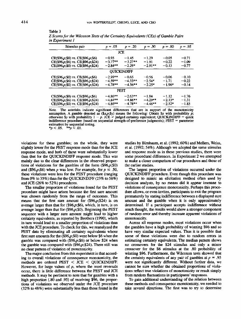
Table 3Z Scores for the Wiicoxon Tests of the Certainty Equivalents (CEs) of Gamble Pairsin Experiment 1

Stimulus pair

CE($96^;$0) vs. CE($96,p;$6)CE($96,p;$6) vs. CE($96,p;$24)CE($96,p;$0) vs. CE($96^;$24)

CE($96,/>;$0) vs. CE($96,/>;$6)CE($96,p;$6) vs. CE($96,/>;$24)CE($96j7;$0) vs. CE($96,/?;$24)

CE($96,p;$0) vs. CE($96,p;$6)CE($96,p;$6) vs. CE($96,p;$24)CE($96,p;$0) vs. CE($96^;$24)

p = .O5 p = .20

JCE

-0.95 -1.45-3.77** -3.27**-2.84** -2.29*

QUICKINDIFF

-2.99** -0.65-4.59** -4.33**-4.78** -4.56**

PEST

-4.86** -2.63**-4.84** -4.86**-4.86** -4.78**

P - . 5 O

-1.29-1.91-2.91**

-0.56-2.54*-2.25*

-1.84-4.29**-4.46**

/> = .80

-0.05-0.22-0.13

-0.06-1.71-1.96*

-1.12-2.13*-2.52*

p = .95

-0.71-1.09-0.77

-0.10-0.22-0.14

-1.76-1.31-1.85

Note. The asterisks indicate significant differences that are in support of the monotonicityassumption. A gamble denoted as ($xj>;$y) means the following: Obtain $x with probability p;otherwise %y with probability 1 — p. JCE = judged certainty equivalent; QUICKINDIFF = quickindifference procedure (based on sequential strength-of-preference judgments); PEST = parameterestimation by sequential testing.*p<.05. * > < . 0 1 .

violations for these gambles; on the whole, they wereslightly lower for the PEST response mode than for die JCEresponse mode, and both of these were substantially lowerthan that for the QUICKINDIFF response mode. This wasmainly due to the clear differences in the observed propor-tions of violations for the gambles of the form ($96,p;$0)and ($96,/>;$6) when p was low. For example, for p < .50,these violations were less for the PEST procedure (rangingfrom 0% to 35%) than for the QUICKINDIFF (23% to 58%)and JCE (26% to 52%) procedures.

The smaller proportion of violations found for the PESTprocedure might have arisen because the first sure amountwas chosen randomly from the range of outcomes. Thismeans that the first sure amount for ($96^;$24) is onaverage larger than that for ($96,p;$6), which, in turn, is onaverage larger than that for ($96^;$0). Beginning the PESTsequence with a larger sure amount might lead to highercertainty equivalents, as reported by Brothers (1990), whichin turn would lead to a smaller proportion of violations thanwith the JCE procedure. To check for this, we reanalyzed thePEST data by eliminating all certainty equivalents whosefirst sure amounts for the ($96^;$0) were below $6 when thegamble was compared with ($96,/>;$6) or below $24 whenthe gamble was compared with ($96,p;$24). There still wasno clear pattern of violation of monotonicity.

The major conclusion from this experiment is that accord-ing to overall violations of consequence monotonicity, themethods are ordered PEST < JCE < QUICKINDIFF.However, for large values of p, where the most reversalsoccur, there is little difference between the PEST and JCEmethods. It may be pertinent to note that for gambles with ahigh proportion (.80 and .95) of receiving $96, the propor-tions of violations we observed under the JCE procedure(32% to 48%) were substantially less than those found in the

studies by Birnbaum, et al. (1992; 60%) and Mellers, Weiss,et al. (1992; 54%). Although we adopted the same stimulusand response mode as in these previous studies, there weresome procedural differences. In Experiment 2 we attemptedto make a closer comparison of our procedures and those ofthe earlier studies.

The largest proportion of violations occurred under theQUICKINDIFF procedure. Even though this procedure wasdesigned to mimic an elicitation method often used bydecision analysts, by no means did it appear immune toviolations of consequence monotonicity. Perhaps this proce-dure allows, or even invites, participants to exit the programprematurely by stating indifference between a displayed sureamount and the gamble when it is only approximatelydetermined. If a participant accepts indifference withoutmuch thought, the results would show a stronger componentof random error and thereby increase apparent violations ofmonotonicity.

Across all response modes, most violations occur whenthe gambles have a high probability of winning $96 and sohave very similar expected values. Thus it is possible thatsome of these violations were due to random errors inestimating certainty equivalents. The median pattern showsno crossovers for the $24 stimulus and only a minorcrossover for the $6 stimulus at the .80 probability ofwinning $96. Furthermore, the Wiicoxon tests showed thatthe certainty equivalents of any pair of gambles at p = .95were not significantly different. Without further data, wecannot be sure whether the obtained proportions of viola-tions reflect true violations of monotonicity or result simplyfrom random fluctuations in participants' responses.

To gain additional understanding of the relation betweenthese methods and consequence monotonicity, we needed totake several directions. The first was to try to determine


whether our somewhat lower—although still high—propor-tion of violations than was found in earlier experiments wasdue to changing from a paper display of the stimuli to one ona computer monitor. We did this in Experiment 2 (although itwas actually run after Experiment 3). A second concern waswhether we could figure out a better way to capture theparticipants1 attention and thereby reduce further the noiselevel. We did this in Experiment 3 by attempting to providemoney amounts and a scenario that would be quite meaning-ful in the real world. And third, there was the seriousproblem of noise in the data, both between and withinsubjects. In Experiment 4 we attempted to estimate thenature and amount of the noise we were encountering and todetermine if it was sufficient to explain, under the hypothesisthat consequence monotonicity holds, the observed viola-tions.

Experiment 2

Of the several procedures used in Experiment 1 (and alsoExperiment 3; see below), the JCE procedure most closelyresembles that used in earlier experiments. Although thisprocedure produced medium to high percentages of viola-tion (between 32% and 48% for the most susceptible gamblepairs), they are somewhat less than those found by Bimbaumet al. (1992) and Mellers, Weiss, et al. (1992) for similarstimuli and conditions (neutral point of view). Severalprocedural differences might have caused the difference inobtained violations. We displayed the stimuli on the com-puter screen as opposed to in a booklet, and the number ofstimuli was smaller (15 stimuli) than in the study by Mellers,Weiss, et al. Although we are not sure whether the displayaffected the results, it is also possible that, instead, thesmaller number of stimuli could have affected the results.With a larger number of stimuli, participants might havedeveloped simplifying estimation strategies. Such strategiesmight be expected to involve calculations that are moreprone to response biases. In fact, Mellers, Weiss, et al.

reported a smaller proportion of violations for fewer stimuli(30 or fewer). In addition, the financial incentive instruc-tions—that 10 gambles would be played to determine theparticipant's score, and those who won the three highestscores would become winners—might have led participantsto be less risk averse or even risk seeking, because the payoffis (he average and only the participants with the top threeaverages would win money. Therefore, in the presentexperiment, we attempted to replicate the studies of Birn-baum et al. and Mellers, Weiss, et al. both in their originalbooklet presentation and in our computer display.

Method

Participants. Thirty-three undergraduate students from theUniversity of California, Irvine and 10 undergraduate studentsfrom the University of Southern California participated in thisexperiment for partial credit for psychology courses.

Stimuli and design. The stimuli were those previously usedand provided to us by Mellers, Weiss, et al. (1992). In total, therewere 77 gambles, 45 of which were test gambles and the remaining32 of which were fillers. Table 4 shows the complete list of the 45test gambles. The 45 test gambles consisted of 3 sets of 15 gambles.For a gamble (x,p;y\ p was either .05, .20, .50, .80, or .95. In thefirst set, x was $96 and y was either $0, $6, or $24. In the second set,x and y were 5 times their values in the first set, and in the third setthey were 10 times their values in the first set

The main factor under investigation was possible differencesbetween the booklet and computer task in testing consequencemonotonicity. All of the conditions were compared within subjects.Each participant received all 77 gambles and performed both tasks.

Stimuli presentation. In the replication of the Mellers, Weiss, etal. (1992) and Bimbaum et al. (1992) experiments, the materialswere presented in a seven-page booklet in which all gambles werepresented as pie charts without numerical probabilities. Dollaramounts were attached to the two segments of the pie chart Thebooklet contained an instruction page, which was followed by apage with 10 warm-up stimuli. The test and filler stimuli werepresented on five subsequent sheets with up to 18 stimuli on eachsheet. The order of the stimulus sheets in the booklet task was

Table 4Stimuli Used in Experiment 2

Number

123456789

101112131415

Gamble

($96,.05;$0)($96,.05;$6)($96,.05;$24)($96,.20;$0)($96,.20;$6)($96,.20;$24)($96,.50;$0)($96,.50;$6)($96,.50;$24)($96,.80;$0)($96,.80;$6)($96,.80;$24)($96.95;$0)($96,.95;$6)($96.96;$24)

Number

161718192021222324252627282930

Gamble

($480,.05;$0)($480v05;$30)($480,.05;$120)($480,.20;$0)($480,.20;$30)($480,.20;$120)($480,.50;$0)($480,.50 $30)($480,.50;$120)($480,.80;$0)($480,.80;$30)($480,.80 $120)($480,.95;$0)($480,.95;$30)($480,.95 $120)

Number

313233343536373839404142434445

Gamble

($960,.05;$0)($960,.05;$60)($960,.05;$240)($960,.20;$0)($960,.20;$60)($960,.20;$240)($960,.50;$0)($960,.50;$60)($960,.50;$240)($960,.80;$0)($960,.80;$60)($960,.80;$240)($960,.95;$0)($960,.95;$60)($960,.95;$240)

Note. A gamble denoted as {%x,p;$y) means the following: Obtain $x with probability p; otherwise$y with probability 1 — p.

416 VON WINTERFELDT, CHUNG. LUCE, AND CHO

varied according to a Latin square design. Each gamble had anumber associated with it. The response sheet had numbered linesfor the 10 warm-up trials and numbered lines for all the gambles.The columns were labeled "Sell" and "Buy." The participantswere instructed to judge the certainty equivalents under either theseller's point of view or the buyer's point of view as follows:

Imagine that you own all the gambles in the experiment Ifyou think the gamble is desirable, write the minimum amount(dollars and cents) you would accept to sell the gamble in thecolumn labeled "Sell." If you think the gamble is undesirable,write the maximum amount (dollars and cents) you would payto avoid playing it in the column labeled "Pay."

Participants wrote the appropriate price for each gamble on thecorresponding number on the response sheets.

The computer-generated stimulus display was identical to thatdescribed in Experiment 1, but only the JCE response mode wasused. The gambles were displayed as shown in Figure 3, both withpie charts and probabilities. The instructions were similar to thosedescribed in Experiment 1 except they omitted the motivation foractually playing some gambles and winning real money. All 77stimuli were presented in random order.

Procedure. The tasks were run in separate sessions, separatedby at least 1 week. Each session lasted for about 45 min. The orderof the two tasks was counterbalanced across participants.

Results

Because we detected no notable differences between thestudents from the two universities, we pooled their data.Table 5 shows the percentages of monotonicity violationsfor the nine pairs of stimuli for which Mellers, Weiss, et al.(1992) and Birnbaum et al. (1992) had found the strongestviolations. The overall percentages of violations were aboutthe same for the booklet task (36%) as for the computer task(37%). They are about the same as those in Experiment 1and again are somewhat lower than those reported byMellers, Weiss, et al. and Birnbaum et al. Table 5 also showsthe percentages of ties, which were surprisingly high in both

tasks. Most ties seemed to occur because participantsrounded responses, for example, to $95 or $90 in the($96,.95;$0) gamble.

The panels in Figure 5 show the median certaintyequivalents of the test gambles in Table 5 as a function of theprobability of winning the higher amount. Although thereare some crossovers at the higher probability end, none isstriking. Table 6 shows the results of Wilcoxon tests for thenine gamble pairs with p = .95 for receiving the largestoutcome. Only one test shows a significant difference in thebooklet task, and this test supports monotonicity. In thecomputer task, two tests show significant differences in thedirection of violating monotonicity, and two show a signifi-cant difference in support of monotonicity. All other testshave nonsignificant p values.

Discussion

With both the computer and booklet tasks, we found someevidence of a violation of consequence monotonicity for thenine stimulus pairs for which previous experiments showedthe strongest violations. Apparently, the introduction of thecomputer procedure neither decreased nor increased thenumber of violations. The observed proportion of violationsin the booklet task (36%) was again somewhat smaller thanthat obtained by Mellers, Weiss, et al. (1992) and Birnbaumet al. (1992). The crossovers at high probability in the plot ofmedian certainty equivalents against the probability toreceive the highest outcome were less pronounced, but threepairs for the computer task were significantly different in thedirection of violations of monotonicity. The percentage ofties (38%) was larger than that found by Mellers, Weiss, etal. (14%) and by Birnbaum et al. (28%) for equivalentconditions. When ties are ignored, the ratio of violations tononviolations was, however, similar to the ratios from theearlier studies.

Table 5Percentages of Participants Violating Consequence Monotonicity or Assigning EqualCertainty Equivalents (Ties) in Experiment 2 (N = 43)

Stimulus pair

($96,.95;$0) vs. ($96,.95;$6)($96,.95;$6) vs. ($96,.95;$24)($96,.95;$0) vs. ($96,.95;$24)

($480,.95;$0) vs. ($96,.95;$30)($480,.95;$3O) vs. ($96,.95;$120)($480,.95;$0) vs. ($96,.95;$120)

($960,.95;$0) vs. ($96,.95;$60)($960,.95;$60) vs. ($96,.95;$240)($960,.95;$0) vs. ($96,.95;$240)

Average

Booklet

Percentviolation

302835

263542

473051

36

Percentties

334435

603333

333533

38

Computer

Percentviolation

474449

282123

404044

37

Percentties

373540

404428

353742

38

Note. A gamble denoted as (5ccj3;$y) means the following: Obtain $x with probability p; otherwise$y with probability 1 — p.

CONSEQUENCE MONOTON1CITY

<$96,p;$x>.

417

O.Z 0.4 0,6 0.8 1-0 0 0.2 0.4 0.6 0.8 1.0


($480,p;$x)

0.2 0.4 0.6 0.8 1.0 0 0.2 0.4 0.S 0.8 1.0Probability to win $480

($96O,p;$x)

0 0.2 0.4 0.6 0.8 1.0 0 0.2 0.4 0.6 0.8 1.0


Figure 5. Median judged certainty equivalents (CEs) for the computer task versus the booklet taskfor the gambles ($96>;&t), ($480,p;$*), and ($960,p;$x), with $x as given in the legends {N = 43).

In summary, this experiment did not show clear differ-ences between the computer and booklet displays in ob-served proportions of violations; however, we did observeconsistently fewer violations than in the earlier experiments.These persistent differences in our experiments, whatevertheir cause, cannot be attributed to such procedural differ-ences as mode of stimulus display or number of stimuli.

Experiment 3

As noted earlier, the purpose of this experiment was toincrease somewhat the realism of the situation. This wasachievable in at least two ways. The first way, used inExperiment 1, was to play out for money some of thegambles after completion of the experiment, thereby provid-ing the participants an opportunity to win more or less

money depending on their choices and on chance. Ourintention was to create monetary incentives, but the stakeswere necessarily rather modest. The other way, pursued inthe present experiment, was to create a somewhat realisticscenario for the gambles but without an actual opportunity toplay. The stakes can be increased under this approach but atthe expense of not providing any direct actual financialincentive. For gambles and stakes we presented hypotheticalstipend offers for amounts between $0 and $9,600. In allother regards, Experiment 3 was identical to Experiment 1.

Method

Participants. Twenty-four undergraduate students from theUniversity of Southern California participated in the experiment,and they received a flat fee of $6 per hour for their participation.


Table 6Z Scores for the Wilcoxon Tests of the Two Certainty Equivalents (CEs) in Experiment 2

Stimulus pair Booklet task Computer task

CE($96,.95;$0) vs. CE($96,.95;$6)CE($96,.95;$6) vs. CE($96,.95;$24)CE($96,.95;$0) vs. CE($96,.95;$24)



-1.26-0.94-1.87*

-0.69-1.46-0.75

-0.94-0.55-1.37

-2.02*-2.40ft-3.25ft

-0.32-0.74-1.20

-1.26-0.94-1.87*

Note. The asterisks indicate significant differences that are in support of the monotonicityassumption. The daggers indicate significant differences that are in violation of the monotonicityassumption. A gamble denoted as ($:c,p;$y) means the following: Obtain %x with probability p;otherwise $y with probability 1 — p.*p<.05. f f p < . 0 1 .

Stimulus presentation and response modes. These were identi-cal to those of Experiment 1 except that all dollar amounts weremultiplied by 100.

Design. The design was identical to that of Experiment 1.Procedure. Participants were introduced to the task by the

experimenter. They were told to imagine that they had to choosebetween two options for obtaining a stipend for the next semester.The first was to accept a sure offer right now, for example, $2,400.The second was to forgo the sure offer and to apply for a secondstipend that carried a larger amount ($9,600); however, there was achance (which varied over .05, .20, .50, .80, and .95) that thesecond stipend would be lowered to either $0, $600, or $2,400.Participants were told to imagine that the uncertainty would beresolved quickly but that once they gave up the sure stipend, itwould be given to someone else and they could not revert to it.

For each response mode, the experimenter guided the partici-pants through some learning trials and then set them up to completeall of the trials of that response mode before they started the nextresponse mode. The experiment lasted from 1 '/2 to 2 hr.

Results

Table 7 shows the overall pattern of violations of conse-quence monotonicity for all stimulus pairs and the threeresponse modes. The overall percentages of violations were14% for PEST, 25% for QUICKINDIFF, and 17% for JCE,which are smaller than those obtained in Experiment 1 andare ordered in the same way. The percentages of violationswere also lower for the gamble pairs with low probabilities

Table 7Percentages of Participants Violating Consequence Monotonicityin Experiment 3 (N = 24)

Procedure

Stimulus pair PEST

48

292933444

1729004

172514

QUICKDSTDIFF

2529172963

817252433

82113244625

JCE

421422933888

2921444

213317

($9,600v05;$0) vs. ($9,600,.05;$600)($9,600,.20;$0) vs. ($9,600,.20;$600)($9,600,.50;$0) vs. ($9,600,.50;$600)($9,600,.80;$0) vs. ($9,600,.80;$600)($9,600,.95;$0) vs. ($9,600,.95;$600)($9,600,.05;$600) vs. ($9,600,.05;$2,400)($9,600,.20;$600) vs. ($9,600,. 20;$2,400)($9,600,.50;$600) vs. ($9,600,.50;$2,400)($9,600,.80;$600) vs. ($9,600,.80;$2,400)($9,600,.95;$600) vs. ($9,600,.95; $2,400)($9,600,.05;$0)vs. ($9,600,.05;$2,400)($9,600,.20;$0) vs. ($9,600,.20;$2,400)($9,600,.50;$0) vs. ($9,600,.50;$2,400)($9,600,.80;$0) vs. ($9,600.80;$2,400)($9,600,.95;$0) vs. ($9,600,.95;$2,4O0)

Average

Note. Agamble denoted ($*,p;$,y) means the following: Obtain %x with probabilityp; otherwise $ywith probability 1 — p. PEST = parameter estimation by sequential testing; QUICKINDIFF = quickindifference procedure (based on sequential strength-of-preference judgments); JCE = judgedcertainty equivalent.

CONSEQUENCE M0N0T0N1OTY 419

of winning $9,600, which were the gamble pairs with thelargest expected-value differences. For the three stimuli thatmost directly tested Mellers, Weiss, et al.'s (1992) violationpattern (i.e., those that involved a .95 probability of winning$9,600), the percentages were largest, but again not as largeas in previous studies: The highest percentages of violationswere found in the QUICKINDIFF procedure (33%, 46%,and 63%), followed by the closely similar JCE (21%, 33%,and 33%), and PEST (29%, 33%, and 25%) procedures.

The three panels of Figure 6 show the median certainty

JCE, ($9600,p;$x)

B

0.2 0.4 0-6 0.8


QUICKINDIFF, ($9600,p;$x)

1.0

8000

6000-

0.2 0.4 0.6 0.8


PEST, ($9600,p;$x)

1.0

8000

6000-

4000-

t 2000-

0-2 0.4 0.6 0.8


1.0

Figure 6. Median certainty equivalents (CEs) for the gambles($9,600jj;$jt), %x being one of $0, $600, or $2,400 (N = 24).JCE = judged certainty equivalent; QUICKINDIFF = quickindiiference procedure (based on sequential strength-of-preferencejudgments); PEST — parameter estimation by sequential testing.

equivalents as a function of the probability of receiving$9,600. When p = .95, we find some crossover in the JCEmode and to a lesser degree in the QUICKINDIFF mode.The crossovers do not occur at all in the PEST procedure.

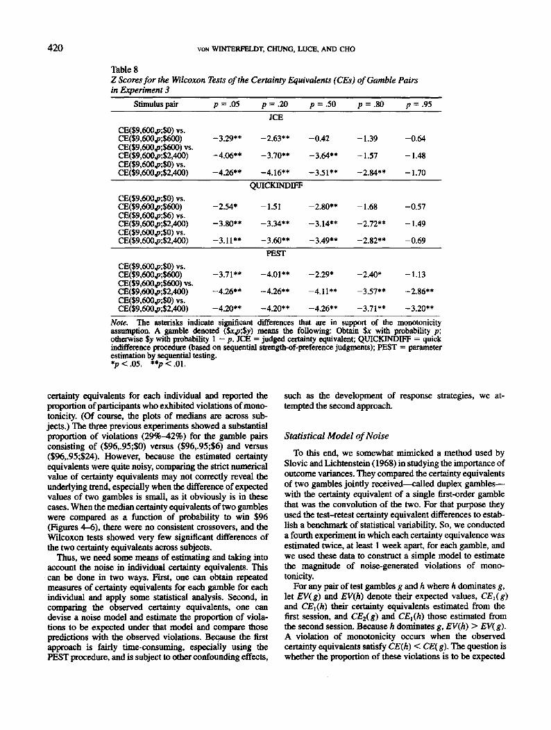
The results of Wilcoxon tests are shown in Table 8. Thecertainty equivalents of any pair of gambles with p = .95were not significantly different for the JCE and QUICKIN-DIFF procedures. For the PEST procedure, the certaintyequivalents for two pairs of gambles at p = .95 weresignificantly different (p < .01) but again in the direction ofsupporting monotonicity. The other results were fairlysimilar to those of Experiment 1, with all significant resultssupporting rather than violating monotonicity. As with thedata in Experiment 1, we reanalyzed the PEST data byeliminating all first sure things below $600 or $2,400,respectively, for the $0 stimulus. There were no changes inthe response pattern.

Discussion

All three response modes in Experiment 3 produced fewerviolations of consequence monotonicity than in Experi-ment 1. For example, violations in the PEST procedure werereduced from 19% to 14%; in the QUICKINDIFF proce-dure, from 30% to 25%; and in the JCE procedure, from31% to 17%. The significant reduction of violations in theJCE mode was observed in ($9,600,p;$0) vs. ($9,600,p;$600) when p = .05 or .20. The QUICKINDIFF procedureshowed somewhat higher proportions of violations than thePEST and JCE procedures, which were nearly the same. Thecrossovers did not appear with the PEST procedure but werestill present with the QUICKINDIFF and JCE procedures.However, none of the certainty equivalent differences in thedirection of violations of monotonicity was significant.Overall, the number of violations of monotonicity wassmaller than in the studies by Mellers, Weiss, et al. (1992)and Birnbaum et al. (1992) except for the QUICKINDIFFprocedure. Because this procedure exhibited in both Experi-ments 1 and 3 appreciably more violations than the JCE andPEST procedures, which may have arisen from a tendency to"early exit," it was dropped from Experiment 4.

Experiment 4

One general problem in studying decision making underrisk is the relatively large amount of noise in the data—bothinconsistencies on repeated presentations within a subjectand differences among subjects. Although estimating cer-tainty equivalents of gambles and constructing the prefer-ence relation by comparing them within subjects may appearto circumvent this specific problem, the fact is that theestimated certainty equivalents are also quite noisy andsubject to similar inconsistencies. These difficulties call intoquestion the precision of inferences we can make from bothJCE and PEST data.

In reporting the degree of violations of monotonicity, wehave focused, as have others, mainly on results from thewithin-subject data analysis: For each pair of gambles, wehave compared the strict numeric value of the estimated


Table 8Z Scores for the Wilcoxon Tests of the Certainty Equivalents (CEs) of Gamble Pairsin Experiment 3

Stimulus pair

CE($9,600,p;$0) vs.CE($9,600#;$600)CE($9,600,p;$600)vs.CE($9,600^;$2,4O0)CE($9,600^;$0) vs.CE($9,600^;$2,400)

CE($9,600^;$0) vs.CE($9,600^;$600)CE($9,600,p;$6) vs.CE($9,600^;$2,400)CE($9,600rf?;$0) vs.CE($9,600^;$2,400)

CE($9t600j?;$0)vs.CE($9,600^;$600)CE($9,600^;$600) vs.CE($9,600rfj;$2,400)CE($9,600rf?;$0) vs.CE($9,600,p;$2,400)

P - . 0 5

-3.29**

-4.06**

-4.26**

-2.54*

-3.80**

-3.11**

-3.71**

-4.26**

-4.20**

p = .2O

JCE

-2.63**

-3.70**

-4.16**

QUICKINDIFF

-1.51

-3.34**

-3.60**

PEST

-4.01**

-4.26**

-4.20**

/? = .5O

-0.42

-3.64**

-3.51**

-2.80**

-3.14**

-3.49**

-2.29*

_4 j2**

-4.26**

p = .80

-1.39

-1.57

-2.84**

-1.68

-2.72**

-2.82**

-2.40*

-3.57**

-3.71**

p = .95

-0.64

-1.48

-1.70

-0.57

-1.49

-0.69

-1.13

-2.86**

-3.20**Note. The asterisks indicate significant differences that are in support of the monotonicityassumption. A gamble denoted ($x,p;$y) means the following: Obtain $x with probability p;otherwise $y with probability 1 — p. JCE = judged certainty equivalent; QUICKINDIFF = quickindifference procedure (based on sequential strength-of-preference judgments); PEST = parameterestimation by sequential testing.*p<.05. **p<M.

certainty equivalents for each individual and reported theproportion of participants who exhibited violations of mono-tonicity. (Of course, the plots of medians are across sub-jects.) The three previous experiments showed a substantialproportion of violations (29%-42%) for the gamble pairsconsisting of ($96\.95;$0) versus ($96,.95;$6) and versus($96V95;$24). However, because the estimated certaintyequivalents were quite noisy, comparing the strict numericalvalue of certainty equivalents may not correctly reveal theunderlying trend, especially when the difference of expectedvalues of two gambles is small, as it obviously is in thesecases. When the median certainty equivalents of two gambleswere compared as a function of probability to win $96(Figures 4-6), there were no consistent crossovers, and theWilcoxon tests showed very few significant differences ofthe two certainty equivalents across subjects.

Thus, we need some means of estimating and taking intoaccount the noise in individual certainty equivalents. Thiscan be done in two ways. First, one can obtain repeatedmeasures of certainty equivalents for each gamble for eachindividual and apply some statistical analysis. Second, incomparing the observed certainty equivalents, one candevise a noise model and estimate the proportion of viola-tions to be expected under that model and compare thosepredictions with the observed violations. Because the firstapproach is fairly time-consuming, especially using thePEST procedure, and is subject to other confounding effects,

such as the development of response strategies, we at-tempted the second approach.

Statistical Model of Noise

To this end, we somewhat mimicked a method used bySlovic and Lichtenstein (1968) in studying the importance ofoutcome variances. They compared the certainty equivalentsof two gambles jointly received—called duplex gambles—with the certainty equivalent of a single first-order gamblethat was the convolution of the two. For that purpose theyused the test-retest certainty equivalent differences to estab-lish a benchmark of statistical variability. So, we conducteda fourth experiment in which each certainty equivalence wasestimated twice, at least 1 week apart, for each gamble, andwe used these data to construct a simple model to estimatethe magnitude of noise-generated violations of mono-tonicity.

For any pair of test gambles g and h where h dominates g,let EV(g) and EV(h) denote their expected values, CEx(g)and CEx(h) their certainty equivalents estimated from thefirst session, and CE2{g) and CEx(h) those estimated fromthe second session. Because h dominates g, EV{h) > EV(g).A violation of monotonicity occurs when the observedcertainty equivalents satisfy CE(h) < CE{ g). The question iswhether the proportion of these violations is to be expected


under the null hypothesis that consequence monotonicityholds but while the data are as noisy as they are.

The goal is to estimate the distribution corresponding tothat null hypothesis. In doing so, we encounter three majorissues. First, what family of distributions should we assume?The distributions over the certainty equivalents are almostcertainty not normal for these gambles. For example, thedistribution of the certainty equivalent of ($96,.95,$JC) withx « $96 probably has a mean of about $80 to $90, istruncated to the right by $96, and has a long left-hand tail.However, we are not interested in this distribution, but in thedifference distribution of two such similarly skewed distribu-tions. Assuming two such distributions, skewed as de-scribed, we simulated the difference distributions and foundthem to be approximately symmetrical and very near tonormal. We therefore assume that the noise distribution ofthe certainty equivalent difference is normal.

Second, what do we take to be the mean difference incertainty equivalents under the null hypothesis of conse-quence monotonicity? One approach is to assume that theparticipants are close to expected-value maximizers and thusthat the mean certainty equivalent difference is close to thedifference in expected values. However, for most partici-pants, the observed certainty equivalents were substantiallyless than the expected value. So an alternate assumption isthat they are expected-utility maximizers with a sharplyrisk-averse utility function. In this case, the certainty equiva-lence difference is roughly three times the expected valuedifference. We therefore conducted two noise analyses: oneusing as the mean the difference of the two expected valuesand the other using as the mean three times that.

Third, what do we take as the standard deviation of thedifference? Here we estimate it from the observed differ-ences in test-retest values of the same gamble, Au(g,g) =CEi(g) - CE2(g)Md&ia(h,h) - CEi(h) - CE2(h), and thenuse that estimate to predict the proportion of noise-inducedviolations.

There are two complications in estimating the variance.First, as we shall see, the CEjS are systematically somewhatlarger than the CE2s. That being so, plus some concern aboutmemory effects within a single session, we therefore pooledall of the differences A2ii(£,g) = - A u = CE2(g) ~ CE{(g)and \l2(hfh) - CEi(k) - CE2(h) and calculated the usualvariance estimate for these pooled observations. Second, thejudgment data exhibited a considerable number of tiedresponses. These ties seemed to occur because participantsoften restricted their responses to either the highest conse-quence ($96) or to nearby multiples of 5 (e.g., $95 or $90).Because any simple continuous noise model does not allowties to occur, we need to estimate the proportions of ties andexclude them in the analysis of noise.

To predict the fraction q of ties, we assumed that theproportion of ties between CE(g) and CE(k) would be equalto the pooled proportion of ties in the test-retest certaintyequivalents of each gamble; that is,

'/2(ties of [CE^g) and CE2(g)) + ties of [CE^h) and CE2(k)]}.

Because of differences between the JCE and PEST proce-

dures, we applied different criteria in predicting the ties intest and retest certainty equivalents. For the JCE method,equal was defined to be exactly equal dollar amounts. Forthe PEST procedure, equal was defined to be an intervalbased on the termination rule that we imposed in estimatingthe certainty equivalent of each gamble. The reason fordoing this is that it is impossible, given the termination ruleof the PEST procedure, to tell the actual sign of thedifference closer than within this interval. Specifically, let #«.and Rh denote the ranges of the test gambles g and h,

\respectively. Then, we treated any differenceCE2(g)\ < Rgf50 and | C£, (h) - CE2 (k)\ <

CEi(g) -as a tie.

The obtained proportions of ties between CE(g) andCE(h) were computed as the pooled proportion of ties in thetest and retest certainty equivalents:

Varies of [CE^g) and CE2(h)] + ties of [CE^h) and CE^g)]}.

Again, we necessarily applied a different criterion for thetwo response modes. As above, for the JCE mode, equal wasdefined to be exactly equal dollar amounts. For the PESTmode, a tie was defined in terms of the following interval:

CEx(g) - CE2(h)\OT\CEX{K) - CE2{g)\

Excluding the ties from consideration, we assume foreach gamble pair and each participant that the differencesA l l 2 ( ^ ) = CEx{h) - CE2(g) and A,,2 = C£,(ft) - CE2{g)are both distributed normally with mean EV(h) — EV(g) (or3 X [EV(hj) - EV(g)]) and variance a2 estimated as thevariance of the pooled across-subject values of the twotest-retest differences A2,i(g,g) and Ali2(A,/i). The predictedproportion of violations of monotonicity, namelyPr[CE(h)- CE(g)<Q], was calculated based on theseassumptions for each participant and each gamble pair, andthese proportions were then averaged over the participants.

If we let q denote the estimated proportion of ties, thenthe predicted proportion of monotonicity violations,excluding the predicted ties from consideration, is(1 - q)Pr[CE(h) - CE(g) < 0].

Method

Participants. Thirty-two undergraduate students from the Uni-versity of Southern California participated in this experiment. Theywere paid $7.50 per hour for their service.

Stimulus presentation and response modes. The stimuli werenine of the test stimuli used in Experiment 2 (see Table 9) plus 20filler items for the PEST procedure. All stimuli were presented on acomputer monitor that generated stimulus displays as described inExperiment 1 (see Figure 3); they were presented in random order.

Procedure. Except for omitting the selection of 10 gamblesand playing them for money, we followed the same procedure as inExperiment 1 for both the JCE and PEST procedures. Their orderwas counterbalanced across participants.

The experiment was run in two sessions, each lasting about 45min, that were separated by at least 1 week. Each session was thesame except for independent randomization.


Table 9Descriptive Statistics of the Test-Retest Certainty Equivalents (CEs)in Experiment 4(N — 32)

Gamble

($96,.95;$0)($96,.95;$6)($96,.95;$24)($480,.95;$0)($480,.95;$30)($480,.95;$120)($960,.95;$0)($960,.95;$60)($960f.95;$24O)

($96,.95;$0)($96,.95;$6)($96,.95;$24)($480,.95;$0)($480,.95;$30)($480,.95;$120)($960,.95;$0)($960,.95;$60)($960,.95;$240)

EV

$91.2$91.5$91.4

$456$458$462$912$915$924

$91$92$92$456$458$462$912$915$924

Mean CEs

Timel

$74.0$70.3$72.3

$361$363$369$752$750$750

$72$74$76$343$356$373$685$690$740

Time 2

JCE$72.8$72.3$74.0

$349$343$358$720$695$725

PEST

$71$72$73$325$333$351$609$652$685

Median CEs

Timel

$80.0$77.5$75.0

$400$400$390$800$812$800

$79.0$80.5$85.8

$377$396$394$757$801$829

Time 2

$80.0$80.0$80.0$350$350$360$750$700$738

$80.5$80.0$79.5$371$370$386$653$787$729

M

12

—2132011325525

123172322763856

d

SD

131719879472175167183

1114139510186251210209

r(31)

0.50-0.65-0.520.821.210.881.031.870.76

0.620.771.151.031.301.431.711.021.51

Note. A gamble denoted ($x,p;$;y) means the following: Obtain $x with probability p\ otherwise %ywith probability 1 — p.EV = expected value; d denotes test-retest difference score; JCE = judgedcertainty equivalent; PEST = parameter estimation by sequential testing.

Results

Table 9 summarizes statistics of the test-ret&t assess-ments (expected values, the means and medians of thecertainty equivalents, and the means and standard deviationsof the differences of certainty equivalents over the twosessions). Note that the estimated certainty equivalents aretypically smaller than the corresponding expected values,and as was noted earlier, the differences in expected valuefor the crucial monotonicity tests are very small. Overall,both the mean and median certainty equivalents are slightlyhigher in the first test than in the second one, although noneof the differences in each gamble pair is significant. Thecertainty equivalents assessed using the JCE procedure aresimilar to those assessed by the PEST procedure. TheWilcoxon test (Table 10) showed no significant violation ofconsequence monotonicity for the JCE procedure and onlyone significant violation for the PEST procedure.

Table 11 shows the predicted proportion of ties estimatedfrom the test-retest data, the predicted violations andnonviolations estimated from the noise model, and thecorresponding observed proportions for the JCE method. Inthis table, the mean of the noise distribution was assumed tobe the difference between the expected values of the twogambles. The expected and observed proportions are veryclose. The chi-square values testing differences betweenobserved and predicted violations, nonviolations, and tiesare not significant for any gamble. Table 12 shows the sameresults under the assumption that the mean of the noisedistribution is three times as large as the expected value

difference. As expected, the predicted proportions of viola-tions are reduced and those of nonviolations correspond-ingly increased. Nonetheless, the results vis-a-vis conse-quence monotonicity are essentially identical to those ofTable 11.

Tables 13 and 14 show the same analyses for the PESTprocedure. The proportion of ties is somewhat larger here

Table 10Z Scores for the Wilcoxon Tests of the 7\vo CertaintyEquivalents (CEs) in Experiment 4

Stimulus pair

CE($96,.95;$0) vs. CE($96,.95;$6)CE($96,.95;$6) vs. CE($96,.95;$24)CE($96,.95;$0) vs. CE($96,.95;$24)CE($480,.95;$0) vs. CE($480,.95;$30)CE($48O,.95;$30) vs. CE($480,.95;$120)CE($480,.95;$0) vs. CE($480,.95;$120)CE($960,.95;$0) vs. CE($960,.95;$60)CE($96O,.95;$60) vs. CE($960,.95;$240)CE($960,.95;$0) vs. CE($960,.95;$240)

z score

JCE-1.73-0.21-0.72-0.73-0.53-1.03-0.24-0.80-0.59

PEST-2.95**-1.51-2.92**-2.48*-2.25|-2.99**-1.36-1.89-2.52*

Note. The asterisks indicate significant differences that are insupport of the monotonicity assumption. The dagger indicates asignificant difference in violation of the monotonicity assumption.A gamble denoted {$x,p\$y) means the following: Obtain $JC withprobability p; otherwise $v with probability I — p. JCE = judgedcertainty equivalent; PEST = parameter estimation by sequentialtesting.*-tp< -05. **/><.01.


Table 11Expected and Observed Percentages ofNonviolation, Violation, and Ties in Monotonicity Tests for the JCE TaskUsing lEV(h) - EV(g)] as the Mean of the Noise Distribution (N = 32)

Gamble pair (g vs. ft)

($96,.95;$0)vs.($96,.95;$6)($96,.95;$6) vs. ($96,.95;$24)($96,.95;$0) vs. ($96,.95;$24)($48O,.95;$O) vs. ($480,-95;$30)($480,.95;$30) vs. ($480,.95;$120)($480,.95;$0) vs. ($480,.95;$120)($960,.95;$0) vs. ($960,.95;$60)($960,.95;$60) vs. ($960,.95;$240)($960,.95;$0) vs. ($960,.95;$240)

Average

Nonviolation

Expected

43464644444545474745

Observed

38504539475238565046

Violation

Expected

42424143404044434242

Observed

48363945383953393842

Expected

161313131616119

1113

Tie

Observed

1414161616995

1312

0.650.480.290.480.131.141.111.450.30

Note. A chi-square of 5.99 is significant at the .05 level. A gamble denoted ($x^?;$y) means the following: Obtain $x with probability p\otherwise $y with probability 1 - p. JCE — judged certainty equivalent.

than for the JCE procedure, which is due to the less stringentdefinition of a tie. However, the overall conclusion is thesame: The noise model provides an excellent fit to theobserved proportions of nonviolations, violations, and ties.

Because we elicited certainty equivalents twice for eachgamble, the participants had two opportunities to violatemonotonicity. Table 15 tabulates the observed proportion of0, 1, and 2 violations for the two procedures. The moststriking result of this tabulation is how rarely participantsviolated monotonicity twice, especially with the PESTprocedure.

Discussion

Experiment 4 yielded violations of monotonicity in aboutthe same proportions as we found in our earlier experiments.For example, there were 37% violations for the JCEprocedure and 34% for the PEST procedure at p = .95 inExperiment 1 versus 42% and 31%, respectively, in Experi-ment 4. Again, both JCE values are somewhat smaller thanthose reported by Mellers, Weiss, et al. (1992) and Birnbaumet al. (1992). We still are not sure why this is so, although a

speculation is offered below. A noise model based ontest-retest certainty equivalent estimates for the same gamblespredicted 12% ties for the JCE procedure and 20% for thePEST procedure. If we exclude ties from consideration, theobserved proportions of violations and nonviolations werenot significantly different from those predicted on the basisof our noise model. Moreover, participants rarely violatedmonotonicity twice. Our conclusion is that given the unfortu-nately noisy character of the data, the observed violations ofconsequence monotonicity are, to a large extent, consistentwith the underlying hypothesis of consequence mono-tonicity.

Conclusions

Earlier tests of consequence monotonicity—one of themost fundamental assumptions of numerous theories ofdecision making under uncertainty—provided mixed re-sults. The earliest, based on a conjecture of Allais (1953),was ambiguous because both monotonicity and reduction ofcompound gambles were involved and it was not clearwhich was the source of trouble. When two gambles in the

Table 12Expected and Observed Percentages ofNonviolation, Violation, and Ties in Monotonicity Tests for the JCE TaskUsing 3 X [EV(h) - EV(g)] as the Mean of the Noise Distribution (N = 32)

Gamble pair (g vs. h)

($96,.95;$0) vs. ($96,.95;$6)($96,.95;$6) vs. ($96,.95;$24)($96(.95;$0) vs. ($96,.95;$24)($480,.95;$0) vs. ($480,.95;$30)($480,.95;$30) vs. ($480,.95;$120)($48O,.95;$O) vs. ($480,.95;$120)($960,.95;$0) vs. ($960,.95;$60)($960,.95;$60) vs. ($960,.95;$240)($960,.95;$0) vs. ($960v95;$240)

Average

Nonviolation

Expected

44495245485046515249

Observed

38504539475238565046

Violation

Expected

40383642373543403739

Observed

48363945383953393842

Expected

161313131616119

1113

Tie

Observed

1414161616995

1312

0.920.120.580.620.011.001.440.040.09

Note. A chi-square of 5.99 is significant at the .05 level. A gamble denoted ($xj>;$y) means the following: Obtain %x with probability p;otherwise $y with probability 1 - p. JCE = judged certainty equivalent; EV = expected value.


Table 13Expected and Observed Percentages of Nonviolation, Violation, and Ties in Monotonicity Tests for the PEST TaskUsing [EV(h) - EV(g)] as the Mean of the Noise Distribution (N = 32)

Gamble pair (g vs. h)

($96,.95;$0)vs.($96,.95;$6)($96,.95;$6) vs. ($96,.95;$24)($96,.95;$0) vs. ($96,.95;$24)($480,.95;$0) vs. ($480,.95;$30)($480,.95;$30) vs. ($480,.95;$120)($480,.95;$0) vs. ($48O,.95;$12O)($960,.95;$0) vs. ($960,.95;$60)($960,.95;$60) vs. ($960,.95;$240)($960,.95;$0) vs. ($960,.95;$240)

Average

Nonviolation

Expected

37394043434636364040

Observed

41424847555847485949

Violation

Expected

36363442404136343737

Observed

33282839343431272231

Expected

27252714171328302323

Tie

Observed

27302314118

22251920

X2(2)

0.180.841.050.171.991.911.602.045.27

Note. A chi-square of 5.99 is significant at the .05 level. PEST = parameter estimation by sequential testing. A gamble denoted (3U,p;$y)means the following: Obtain $* with probability/?; otherwise $y with probability 1 — p. EV = expected value.

consequence monotonicity condition were compared di-rectly, the monotonicity assumption was not rejected (Broth-ers, 1990; Bimbaum & Sutton, 1992; Kahneman & Tversky,1979). However, when research participants directly judgedthe certainty equivalents of gambles, and the preferencerelations of gamble pairs were constructed indirectly bycomparing the estimated certainty equivalents, consequencemonotonicity appeared to be consistently violated, espe-cially for gambles involving very small probabilities ofreceiving zero or near-zero outcomes (Birnbaum, 1992;Birnbaum & Sutton, 1992; Birnbaum et al., 1992; Mellers,Weiss, et al., 1992). The present series of four experimentswas conducted in an attempt to clarify the relation betweenthe choice and the judged certainty equivalent results.

We conjectured that monotonicity violations may be moreprevalent in judged certainty data than in choice databecause judged certainty equivalents possibly involve simpli-fying calculations. We were motivated, men, to test thedependence of violations on response modes. We studiedthree: judged certainty equivalents, or JCE, and two types ofchoice-based ones, PEST and QUICKINDIFF. Although the

JCE response mode in Experiment 1 produced more viola-tions than the other two for the gambles with low probabili-ties of receiving $96, this pattern was not replicated inExperiment 3, where the stakes were increased by a factor of100 and a somewhat more realistic scenario was used. Inboth experiments, all response modes produced some frac-tion of violations for the gambles when the probability ofreceiving the maximum outcome was large. There were nonoticeable differences in the proportion of observed viola-tions between the JCE and PEST response modes. When themedian estimated certainty equivalents of two gambles werecompared as a function of probability to win $96 (or$9,600), there were no consistent crossovers, and the resultsof Wilcoxon tests did not reject consequence monotonicitybetween the two certainty equivalents for any of the gamblepairs in Experiments 1 and 3. Indeed, for the PESTprocedure, the Wilcoxon tests provided significant supportfor consequence monotonicity in 10 of 15 tests in Experi-ment 1 and in 14 of 15 tests in Experiment 3, with all othertests not being significant.

The QUICKINDIFF response mode was an attempt to

Table 14Expected and Observed Percentages of Nonviolation, Violation, and Ties in Monotonicity Tests for the PEST TaskUsing 3 X [EV(h) - EV(g)] as the Mean of the Noise Distribution (N = 32)

Gamble pair (g\s.h)

($96,.95;$0) vs. ($96,.95;$6)($96,.95;$6) vs. ($96,.95;$24)($96,.95;$0) vs. ($96,.95;$24)($480,.95;$0) vs. ($480,.95;$30)($480,.95;$30) vs. ($480,.95;$120)($480,.95;$0) vs. ($480,.95;$ 120)($96O,.95;$0) vs. ($960,.95;$60)($96O,.95;$60) vs. ($960,.95;$240)($960,.95;$0) vs. ($960,.95:$24O)

Average

Nonviolation

Expected

39434545465137394343

Observed

41424847555847485949

Violation

Expected

35322841373735323435

Observed

33282839343431272231

Expected

27252714171328302323

Tie

Observed

27302314118

22251920

X2(2)

0.050.420.190.081.280.941.401.263.58

Note. A chi-square of 5.99 is significant at the .05 level. A gamble denoted (&c,p;$y) means the following: Obtain $x with probability p;otherwise $v with probability 1 - p. PEST = parameter estimation by sequential testing. EV = expected value.

CONSEQUENCE MONOTONIOTY 425

Table 15Observed Distribution ofO, 1, and 2 Violationsof the Monotonicity Assumption (N — 32)

Gamble pair

JCE

($96,.95;$0) vs. ($96,.95;$6)($96,.95;$6) vs. ($96,.95;$24)($96,.95;$0) vs. ($96,.95;$24)($480,.95;$0) vs. ($48O,.95;$30)($480,.95;$30) vs. ($480,.95;$120)($480,.95;$0)vs. ($480,.95;$120)($960,.95;$0) vs. ($960,.95;$60)($960,.95;$60) vs. ($960,.95;$240)($960,.95;$0) vs. ($960,.95;$240)

AveragePEST

($96,.95;$0) vs. ($96,.95;$6)($96,.95;$6) vs. ($96,.95;$24)($96,.95;$0) vs. ($96,.95;$24)($48O,.95;$O)vs. ($48O,.95;$3O)($480,.95;$30) vs. ($480,.95;$120)($480,.95;$0) vs. ($480,.95;$120)($96O,.95;$O) vs. ($960,.95;$60)($960,.95;$60) vs. ($960,.95;$240)($960,.95;$0) vs. ($960,.95;$240)

Average

0

511117

13105

10109

9121449

1010141511

Observedviolation count

1

23191723151922202020

23191628222121171720

2

4242435223

0120111101

Note. A gamble denoted ($x,p;$y) means: Obtain $x with probabil-ity p; otherwise $y with probability 1 - p. JCE = judged certaintyequivalent; PEST = parameter estimation by sequential testing.

develop a faster procedure than that provided by PEST forestimating the choice-induced certainty equivalents. How-ever, QU1CKINDIFF exhibited appreciably more violationsof consequence monotonicity than the other two procedures.Perhaps this is because it easily allows participants to exitthe program before actual indifference is established. Wecannot recommend its use as now formulated, but furtherinvestigation of procedures faster than PEST is needed.

Another fast technique that is sometimes used (Birnbaumet al., 1992; Tversky & Kahneman, 1992) to estimatecertainty equivalents involves participants' marking whichof a list of sure consequences are better than a gamble.Although this is nominally choice based, we are suspiciousthat it is a judgment procedure in disguise.

Unexpectedly, in both Experiments 1 and 3 under the JCEprocedure a smaller proportion of violations was exhibitedthan was reported in the earlier studies by Birnbaum et al.(1992) and Mellers, Weiss, et al. (1992). To investigate thepossibility that our using a computer monitor presentationrather than a booklet of drawings of pie diagrams might havebeen the source of this difference, we conducted Experiment2 to compare the two JCE presentations. We again foundlower proportions of violations in both presentations than inthe earlier studies. In the booklet task, the Wilcoxon testsshowed no significant violations of monotonicity for any ofthe gamble pairs that were suspected to produce violations.In the computer task, two of the nine tests showed significant

violations of monotonicity. So, the question remains: Whyare we getting smaller, nonsignificant proportions of viola-tions? One possibility, which we did not investigate, is thatthe earlier data were collected in classroom situationswhereas ours were in individual laboratory settings. Perhapsthe personal attention given to our participants to ensure thatthey understood what was to be done may have made themmore careful.

To test whether the observed proportions of violations ofboth JCE and PEST response modes really can be explainedsimply by the (apparently inherent) noise in estimatingcertainty equivalents, we proposed a noise model utilizingthe test-retest data collected in Experiment 4. When tieswere excluded from consideration, the predicted proportionsof violations from the noise model were not significantlydifferent from those observed in both the JCE and PESTprocedures. In addition, when participants had two opportu-nities to violate consequence monotonicity with the samegamble pair, they very rarely did so. Our conclusion,therefore, is that when the noisy nature of the data are takeninto account, we cannot reject the hypothesis of conse-quence monotonicity.

Although we were unable to reject consequence monoto-nicity for either the judged or the PEST-based certaintyequivalents using our noise model, that model has at leasttwo rather severe limitations. First, we used test-retest datato estimate the number of ties to be added to the continuousnoise model. These same data were also used to estimate thevariance of the underlying noise distribution across subjects.The ideal way to analyze the noise underlying our estimatesof certainty equivalents would be to repeatedly measure itand to apply statistical tests for each individual. Althoughideal, it is impractical in this context, especially the PESTone, to obtain a sufficiently large sample of individualtest-retest data. One likely difficulty in pursuing this ap-proach lies in how to reduce memory effects without usingmany filler gambles. In the PEST procedure, it is impossibleto test a large set of gambles in one or two successivesessions.

Second, the certainty equivalents estimated in the retestsession, which was performed at least 1 week later than thetest session, were consistently less than those of the testones. It would be interesting to obtain the test-retestcertainty equivalents in the same session or, if that is notfeasible, in sessions separated by less time than a week.

Despite a fairly large proportion of observed violations ofconsequence monotonicity, which seems to be largely due tothe level of noise in estimating them, we conclude from theseveral analyses that consequence monotonicity cannot berejected. This is true for both judged certainty equivalentsand PEST-determined certainty equivalents. The fact thatthere is little difference in the proportions of violations ofconsequence monotonicity between the two procedures andthe greater ease of collecting JCE judgments seem torecommend the JCE procedure over the PEST procedure.Nonetheless, we urge caution in using judged certaintyequivalents to test choice-based theories of decision making.For one thing, the median data slightly favor the PEST


procedure for reducing violations of consequence monotonic-ity; for a second, the judged estimates have a seriousrestriction in the numbers used, and so many ties occur; andfor a third, we know from the preference-reversal experi-ments that judged certainty equivalents do not always agreewith choices.

References

AJlais, M. (1953). Le comportement de I'homme rationnel devantle risque: Critique des postulats et axiomes de l'lcole Ameri-caine. Econometrica, 21, 503-546.

Allais, M., & Hagen, O. (Eds.). (1979). Expected utility hypothesisand the Allais'paradox. Dordrecht, The Netherlands: Reidel.

Birabaum, M. H. (1992). Violations of monotonicity and contex-tual effects in choice-based certainty equivalents. PsychologicalScience, 3, 310-314.

Bimbaum, M. H., Coffey, G., Mellers, B. A., & Weiss, R. (1992).Utility measurement: Configural-weight theory and the judge'spoint of view. Journal of Experimental Psychology: HumanPerception and Performance, 18, 331-346.

Birnbaum, M. H., & Sutton, S. £. (1992). Scale convergence andutility measurement. Organizational Behavior and Human Deci-sion Processes, 52, 183-215.

Bostic, R., Herrnstein, R. J., & Luce, R. D. (1990). The effect on thepreference-reversal phenomenon of using choice indifferences.Journal of Economic Behavior and Organization, 13, 193-212.

Brothers, A. J. (1990). An empirical investigation of some proper-ties that are relevant to generalized expected-utility theory.Unpublished doctoral dissertation, University of California,Irvine.

Chew, S. H., Kami, E., & Safra, Z. (1987). Risk aversion in thetheory of expected utility with rank dependent probabilities.Journal of Economic Theory, 42, 370-381.

Gilboa, I. (1987). Expected utility with purely subjective non-additive probabilities. Journal of Mathematical Economics, 16,65-88.

Grether, D. M., & Plott, C. R. (1979). Economic theory of choiceand the preference reversal phenomenon. American EconomicReview, 69, 623-638.

Kahneman, D., & Tversky, A. (1979). Prospect theory: An analysisof decision under risk. Econometrica, 47, 263-291.

Lichtenstein, S., & Slovic, P. (1971). Reversals of preferencebetween bids and choices in gambling decisions, Journal ofExperimental Psychology, 89, 46-55.

Luce, R. D. (1988). Rank-dependent, subjective expected-utilityrepresentations. Journal of Risk and Uncertainty, 1, 305-332.

Luce, R. D. (1991). Rank- and sign-dependent linear utility modelsfor binary gambles. Journal of Economic Theory, 53, 75-100.

Luce, R. D. (1992). Where does subjective-expected utility faildescriptively? Journal of Risk and Uncertainty, 5, 5-27.

Luce, R. D., & Fishburn, P. C. (1991). Rank- and sign-dependentlinear utility models for finite first-order gambles. Journal ofRisk and Uncertainty, 5, 29-59.

Luce. R. D., & Fishburn, P. C. (1995). A note on derivingrank-dependent utility using additive joint receipts. Journal ofRisk and Uncertainty, 11, 5-16.

Mellers, B. A., Chang, S., Birnbaum, M. H., & Ordote, L. D.(1992). Preferences, prices, and ratings in risky decision making.Journal of Experimental Psychology: Human Perception andPerformance, 18, 347-361.

Mellers, B., Weiss, R., & Birnbaum, M. H. (1992). Violations ofdominance in pricing judgments. Journal of Risk and uncer-tainty, 5,73-90.

Quiggin, J. (1982). A theory of anticipated utility. Journal ofEconomic Behavior and Organizations, 3, 324-343.

Quiggin, J. (1993). Generalized expected utility theory: Therank-dependent model. Boston: Kluwer Academic.

Savage, L. J. (1954). The foundations of statistics. New York:Wiley.

Schmeidler, D. (1986). Subjective probability and expected utilitywithout additivity. Econometrica, 57,571-587.

Segal, U. (1987). Some remarks on Quiggin's anticipated utility.Journal of Economic Behavior and Organization, 8, 145-154.

Segal, U. (1989). Anticipated utility: A measure representationapproach. Annals of Operations Research, 19, 359-373.

Slovic, P., & Lichtenstein, S. (1968). Importance of variancepreferences in gambling decision. Journal of ExperimentalPsychology, 78,646-654.

Slovic, P., & Lichtenstein, S. (1983). Preference reversals: Abroader perspective. American Economic Review, 73, 596-605.

Tversky, A., & Kahneman, D. (1992). Advances in prospect theory:Cumulative representation of uncertainty. Journal of Risk andUncertainty, 5, 204-217.

Tversky, A., Sattah, S., & Slovic, P. (1988). Contingent weightingjudgment and choice. Psychological Review, 95, 371-384.

Tversky, A., Slovic, P., & Kahneman, D. (1990). The causes ofpreference reversal. American Economic Review, 80, 204-217.

Wakker, P. P. (1989). Additive representations of preferences: Anew foundation of decision analysis. Dordrecht, The Nether-lands: Kluwer Academic.

Wakker, P. P., & Tversky, A. (1993). An axiomatization ofcumulative prospect theory. Journal of Risk and Uncertainty, 7,147-176.

Yaari, M. E. (1987). The dual theory of choice under risk,Econometrica, 55, 95-115.

Received April 7,1993Revision received July 29,1996

Accepted July 29,1996

Journal of Experimental Psychology: 1997, Vol, 23, No ... Sattah, & Slovic, 1988). That being the...

Documents

Transcript of Journal of Experimental Psychology: 1997, Vol, 23, No ... Sattah, & Slovic, 1988). That being the...