JOURNAL OF ECONOMIC THEORY 20, 381-408 (1979) - SFU.cakkasa/HarrisonKreps_79.pdf · JOURNAL OF...

JOURNAL OF ECONOMIC THEORY 20, 381-408 (1979)

Martingales and Arbitrage in Multiperiod Securities Markets

J. MICHAEL HARRISON AND DAVID M. KREPS

Graduate School of Business, Stanford University, Stanford, California 94305

Received May 24, 1978; revised February 9, 1979

1. INTRODUCTION AND SUMMARY

We consider in this paper some foundational issues that arise in conjunction with the arbitrage theory of option pricing. In this theory, initiated by Black and Scholes [4], one takes as given the price dynamics of certain securities (such as stocks and bonds). From these, one tries to determine the prices of other contingent claims (such as options written on a stock) through arbitrage considerations alone. That is, one seeks to show that there exists a single price for a specified contingent claim which, together with the given securities prices, will not permit arbitrage profits.

This paper contains a fairly general theory of contingent claim valuation along these lines. We begin in Section 2 with a general theory of arbitrage in a two-date economy with uncertainty. The dates are indexed t = 0, T. A probability space (Q, F, P) if given, where points w E .Q represent states of the world. The probability measure P can be interpreted for now as a set of unanimously held subjective probability assessments concerning the state of the world. There is a single consumption good, the numeraire, and agents are interested in certain consumption at date zero and state contingent consumption at date T. Thus we consider consumption bundles of the form (r, x) E R x X, where R is the real line and X is a space of random variables on (Q, F>. Here (r, x) represents r units of consumption at date zero and x(o) units of consumption at date T if the state is w.

Agents are specified by their preferences over R x X, these being interpreted as preferences for net trade vectors. More explicitly, an agent’s preferences are given by a complete and transitive binary relation 2 on R x X that is assumed to be convex, continuous and strictly increasing, in a sense to be made precise.

A price system for this economy is a pair (M, 7r) where M is a subspace of X and r is a linear functional on M. The interpretation is that agents can purchase any bundle (r, m) E R x Mat a price (in units of date zero consumption) of r + n(m). In taking M to be a subspace and r a linear functional, we are assuming frictionless markets (no transaction costs and unrestricted

381 OO22-O531/79/030381-28$O2.00/0

Copyright Q 1979 by Academic Press, Inc. All tights of reproduction in any form reserved.

382 HARRISON AND KREPS

short sales). A price system (M, PT) is said to be viable if there exists an agent (represented by 2) and a bundle (r*, m*) E R x M such that

r* + I < 0 and (r*, m*) 2 (r, m) for all (r, m) E R x A4

such that r + +EZ) < 0. (1.1)

Since (r, m) is a net trade vector, the condition P + n(m) < 0 is the agent’s budget constraint. Thus (1.1) is a necessary and sufficient condition for (M, r) to be viable as a model of an economic equilibrium. An equivalent condition is established in Theorem 1. A price system (M, 7r) is shown to be viable if and only if there exists a continuous and strictly positive extension of 7r to all of X.

Given a viable price system (M, r) and a contingent claim x E X, what price in date zero consumption might x command? If x sold for price p, agents could purchase any claim of the form m + hx at a price of r(m) + hp (for m E M and X real). It is natural, therefore, to say that price p for x is consistent with (M, Z-) if this augmented price system is viable. Claim x is said to be priced by arbitrage if there is a unique price for x that is consistent with (M, n). In this case, the unique consistent price is called the arbitrage value of x. As a corollary to Theorem 1, we find that x is priced by arbitrage if and only if it has the same value under every continuous and strictly positive linear extension of r to all of X, in which case that common value is the arbitrage value of the claim.

In Section 3 these general concepts are adapted to models of multiperiod securities markets. Given $2, F, P) and T as before, a securities market model consists of a set T C [0, T] of trading dates, an information structure represented by an increasing family of sub-o-algebras, and a vector stochastic process 2 = (Z(t); t E T} that gives the prices of a finite collection of traded securities for every date t E T and state o E J2. We assume that one of these securities is a riskless bond and that the rate of return to this bond is zero. (This entails no significant loss of generality, as we discuss in Section 7.)

We next consider how agents can use the traded securities to transfer consumption between dates zero and T. We require (somewhat arbitrarily) that agents employ only what we call simple trading strategies. The key restriction is that an agent may change the contents of his portfolio of securities at only a finite number N of prespecified trading dates, although N may be arbitrarily large (if T is infinite). A simple trading strategy is said to be self-financing if the cost of any security purchase after date zero is exactly equal to the revenue generated by a simultaneous sale of some other securities, and if any sale is similarly matched by some purchase. As these trading strategies neither require nor generate funds between dates zero and T, they represent the means available to agents for transfering consumption between dates zero and T. They give rise to a space of implicitly marketed claims A4

MARTINGALES AND ARBITRAGE 383

and prices 7~ for these claims, to which the results of Section 2 can be applied. Thus we say that a securities market model is viable if the corresponding price system (M, n) is viable, that a contingent claim’s price is determined by arbitrage from a viable securities market model if its price is determined from the corresponding (M, v), and so on.

For a securities market model as above, an equivalent martingale measure is a probability measure P* on (Q, F) having three properties. The first is technical. The second is that P and P* are equivalent, meaning that P*(B) > 0 if and only if P(B) > 0. The third property is that the price process Z becomes a (vector) martingale when P is replaced by P*. Thus the conversion from P to P* represents a redistribution of probability mass that causes every security to earn (in expected value) at the riskless rate zero without changing the set of events that receive positive probability. Let (M,r) be the price system corresponding to a given securities market model. Theorem 2 establishes a one-to-one correspondence between equivalent martingale measures P* and those continuous and strictly positive linear functionals # which extend n to all of X. This correspondence is given by

#(x) = E*(x) for x E X, and P*(B) = #(la) for B EF,

where E* is the expectation operator associated with P*. When combined with earlier results, this yields the following. A securities market model is viable if and only if there exists at least one equivalent martingale measure for it. For a viable securities market model, the price of a contingent claim x is determined by arbitrage if and only if x has the same expectation under every equivalent martingale measure, in which case the arbitrage value of x is that common expectation.

To illustrate these propositions, we apply them in Section 4 to the case where both Q and T are finite. In Section 5 we consider the much more complex case where T = [0, T] and Z is a vector diffusion process. With mild regularity assumptions, it is shown (Theorem 3) that there exists a unique equivalent martingale measure. Thus the model is viable, and the price of every contingent claim (depending on the complete price history in an arbitrary way) is determined by arbitrage. The conversion to the equivalent martingale measure is accomplished by simply zeroing out the drift in the original model. Thus, in principle, all arbitrage values can be computed.

The theory developed in Section 3 is profoundly affected by our restriction to simple trading strategies. This restriction is made for technical reasons and cannot be completely justified on economic grounds. In Section 6 we discuss various alternative approaches that might be taken, and we illustrate the pitfalls that must be avoided if one is to model directly continuous trading (or otherwise expand the class of trading strategies permitted to agents).

Extensions of our theory are discussed in Section 7. We indicate how to apply our results when there is not a riskless security with rate of interest


zero, when contingent claims may pay off at multiple and/or varying dates, and when one wishes to value an option (such as an American put) where the holder has some discretion as to the time and/or amount of payoff. Also, we discuss a technical matter concerning the topology in which agents’ preferences are a.ssumed to be continuous.

Section 8 contains some miscellaneous concluding remarks. For the most part, comments on connections with the extant literature are reserved for this section.

2. VIABILITY AND ARBITRAGE

As outlined in Section 1, a probability space $2, F, P) and two dates (t = 0 and t = T) are fixed. For the space X of contingent claims to consumption at date T, we shall take the space of F-measurable random variables that are square integrable. That is, we take X = L2(Q, F, P). This restriction of attention to square integrable contingent claims is made for expositional and mathematical ease. It is not necessary for most of the development that follows, and extensions are discussed in Section 7.

Agents are characterized by their preferences on the space of net trades, R x X. Such preferences are represented mathematically by complete and transitive binary relations 2 on R x X. (In the usual fashion, > denotes strict preference defined from 2.) The preferences of agents in this economy are assumed to satisfy three requirements. First, they are convex.

For all (Y, x) E R x X, the set {(r’, x’) E R x X : (r’, x’) 2 (r, x)} is convex. (2.1)

Second, they are continuous in the following sense. Let T be the product topology on R x X derived from the Euclidean topology on R and the L2 norm topology on X.

For all (r, x) E R x X, the sets {(r’, x’) E R x X : (r’, x’) 2 (r, x)}

and ((r’, x’) E R x X : (r, x) 2 (r’, x’)} are T closed. (2.2)

Third, they are strictly increasing in the following sense. Let Xf be the set of contingent claims x satisfying P(x 2 0) = 1 and P(x > 0) > 0.

For all (r, x) E R x X, r’ E (0, cc) and x’ E X+, (r + r’, x) > (r, x)

and (r, x + x’) > (r, x). (2.3)

In words, if we start with a net trade (r, x) and add to it either a positive amount of time zero consumption or a claim x E X+ (which does not decrease time T consumption and may increase it), then the resulting net trade vector


is strictly preferred to the original. The set of complete and transitive binary relations 2 on R x X that satisfy (2.1), (2.2) and (2.3) is denoted A. Thus A represents the class of conceivable agents.

To illustrate the role of the probability measure Pin our theory, we consider the following special case. Suppose that there exists a probability measure Q on (D, F) and a function u : R x R + R such that 2 is given by

(r, x) 2 (r’, x’) if Iu(r, X(W)) Q(dw) 3 /u(r', X’(W)) Q(h).

(This assumes that u and Q are sufficiently well behaved so that all integrals of the indicated form exist and are finite.) For 2 to be in A it is sufficient that u be concave and strictly increasing and grow in absolute value at no more than quadratic rate, that Q and P have the same null sets, and that dQ/dP be bounded. This example shows that P plays three roles. It determines the space X of contingent claims, it determines the continuity requirement for 2 E A, and through its null sets it plays a role in the requirement that 2 E A be strictly increasing.

A price system is a subspace M of X and a linear functional rr on M. The interpretation is that in this economy, agents are able to buy and sell some contingent claims at a cost in date zero consumption. The markets in which this can be done are frictionless, meaning that there are no transaction costs and no restrictions on short selling. Thus M represents the subspace of marketed contingent claims (which will be smaller than X if markets are incomplete), and TT gives the prices for claims m E M in units of date zero consumption.

Given a price system (M, ‘rr), is it viable as a model of economic equilibrium for agents from the class A? Formally, a price system (M, n) is said to be viable if there exists some 2 E A and (r*, m*) E R x M such that

r* + n(m*) < 0 and (r*, m*) 2 (r, m) for all (r, m) E R x M

such that r + n-(m) < 0. (2.4)

This says that there is some agent from the class A who, when choosing a best net trade subject to his budget constraint r + r(m) < 0, is able to find an optimal trade. The necessity of this condition is clear. It is also sufficient in the following sense. Given an agent 2 E A and (r*, m*) E R x M satisfying (2.4), define a relation 2’ on R x X by

(r, x) 2’ (r’, x’) if (r + r*, x + m*) 2 (r’ + r*, x’ + m*).

Then 2’ E A, and an agent with preferences 2’ weakly prefers (0,O) to every net trade (r, m) E R x M such that r + n-(m) < 0. Thus (M, TT) is an equilibrium price system for an economy populated by agents from the class


A. In an economy where all agents have preferences k’, at prices r every agent is content to remain at his endowment point.

The following theorem characterizes viable price systems in terms of continuous (in the L2 norm topology) linear functionals on X. Such a linear functional $ is said to be strictly positive if 4(x) > 0 for all x E X--. Let Y denote the set of all continuous and strictly positive linear functionals on X.

THEOREM 1. A price system (M, T) is viable if and only if there exists cln extension of TT to all of X that lies in Y.

(We use the notation # 1 M to denote the restriction of I$ to the subspace M, and thus the condition can be rephrased as follows. There exists $J E Y such that # j A4 = n.)

Proof. Suppose (M, 7r) are such that there exists # E Y satisfying # 1 M : 71. Then define 2 on R x X by

(r, x) 2 (r’, x’) if r + z/(x) 3 r’ + #(x’).

It is easy to see that the relation 2 so defined is in A and that this 2 and the choice (r*, m*) = (0, 0) satisfy (2.4). Thus (M, n) is viable.

Suppose (M, r) is viable. Let z E A and (r*, m*) be such that (2.4) holds. Previous discussion shows that (r*, m*) = (0,O) may be assumed without loss of generality. Define

and

G = {(r, x) E R x X : (r, x) > (0, 0))

H = {(r, m) E R x A4 : r + n(m) < O}.

The sets G and H are disjoint because of (2.4), both are convex (G because preferences are convex) and G is open (because preferences are continuous). Thus there exists a nontrivial continuous linear functional q5 on R :,’ A4 such that #(r, X) 3 0 for (r, x) E G and d(r, x) < 0 for (r, x) E H. This is one version of the separating hyperplane theorem; see Holmes [I 1, p. 631.

We claim that &I, 0) > 0. To see this, note that there is some (r’, x’) such that r$(r’, x’) > 0 because 4 is nontrivial. Since 2 E A, we have (1,0) > (0,O). Thus by continuity of 2, there exists X > 0 sufficiently small so that (1 - hr’, -Xx’) > (0,O). Therefore

+(I - hr’, --hx’) = +(I, 0) - h$(r’, x’) > 0,

and $<I, 0) > X4< r’, x’) > 0. Renormalize 4 so that #J( 1,0) = 1, and write +(r, x) = r + $(x), where # . is a continuous linear functional on X.


We claim that 9 is strictly positive. For x E X+, we have (0, x) > (0, 0), thus there exists h > 0 such that (--h, x) > (0,O). This implies #(x) - h > 0 or #(x) b X > 0.

We claim that t,+4 1 A4 = V. For m E M, note that (-n(m), m) and (r(m), -m) are both in H, and thus 0 = +(?r(m), -m) = r(m) - #(m), or n(m) = 4(m). This completes the proof.

This equivalent characterization of viability has a partial equilibrium- general equilibrium flavor to it. Imagine an economy where markets exist for all claims x E X, one portion of that economy being the market where claims m E M can be bought and sold at prices 7~. Then these prices must be part of a general equilibrium system of prices # for all of X. And as agents come from the class A, these general equilibrium prices must be continuous and strictly positive.

Suppose a viable price system (M, r) is given. At what prices might some other claim x $ M sell for? If x sold at a price p, agents would be able to purchase any claim m + hx E span(M u {x}) at a price n(m) + Ap. Writing M’ for span (A4 u {x}) and r’ for the linear functional r’(m + Xx) = a(m) + hp, it is natural to say that price p for x is consistent with the price system (M, n) if (M’, rr’) is viable. Immediately from Theorem 1 we have the following corollary.

COROLLARY 1. If a price system (.M, n) is viable, then for all x E X there exists some price that is consistent with (M, T). Moreover, for viable (M, 7~), the set of prices for x consistent with (M, n) is the set {#(x) : # E Y and $hIM=7r).

When there is a single price for a claim x consistent with (M, r), we say that the price of x is determined by arbitrage from (M, r), and this unique price for x is called the arbitrage value of x (determined from (M, 7)).

COROLLARY 2. If a price system (A4, T) is viable, then the price of x E X is determined by arbitrage if and only if the set {3(x) : # E Y and # 1 M = T} is singleton, in which case that single element is the arbitrage value of x.

Given a viable price system (M, 7~), let i@ be the set of all contingent claims whose prices are determined by arbitrage. Let 6(x) denote the arbitrage value of claim x E &. If X is finite dimensional (which will be the case if Q is finite), it can be shown that l@ = M. If X is infinite dimensional (which will typically be the case if D is infinite), it follows from Corollary 2 that J?Z contains at least the T closure of M, and it may contain other claims as well. Because our primary interest here is in multiperiod securities markets, we shall not further develop the general concepts of viability and arbitrage that have been advanced. A great deal more can be said, however, and the interested reader is directed to [12].


3. SECURITIES MARKET MODELS

As stated earlier, the additional primitive objects required for our securities market model are a set of trading dates, an information structure, and a price process. The trading dates are a set T C [0, T] with 0, T E T. Interpret T as a collection of points in time at which certain (as yet unspecified) securities can be traded. The terms discrete time and continuous time refer to the cases where T is finite and where T = [0, T], respectively.

The information structure is given by an increasing family of sub-o-algebras (Ft ; t E T}. We assume for convenience that F, is the trivial u-algebra ( ia, Sz} and that FT = F. Interpret I;t as the class of all events B such that agents will be able to tell at time t whether the true state of the world is in B. In other words, Ft represents the information available at time t. The price process is a (K + I)-dimensional stochastic process 2 = {Z(t); t E T} which is adapted to {Ft}. The components of Z(t) are denoted Z,(t) for k = 0, l,..., K. Interpret K + 1 as the number of securities traded in this market, with Z,(r, w) representing the price of security k at time t if the state is w. The assumption that Z is adapted to (F,} simply means that among the information available at time t are the prices then prevailing for all traded securities. We assume for now that these securities do not generate any revenue such as dividends. Also, we assume that Z,,(t, w) = 1 for all t and w. The latter assumption means that security zero is a riskless asset (a bond) with interest rate zero. This seems highly restrictive but is not, as we shall discuss in Section 7. Finally, we assume that E(Zk2(t)) < cc for all t E T and k = I,..., K.

Hereafter we refer to the probability space (Q, F, P), the set of trading dates T, the information structure {F,}, and the price process 2 together as a securities market model.

For a concrete example, fix some T > 0, set T = [0, T] and let ($2, F, P) be a probability space on which is defined a standard (zero drift and unit variance) Brownian Motion (W(t); 0 < t < T>. Let Ff be the u-algebra generated by (W(U); 0 < u < t} and assume F = FT . Define Zo(t) = 1 and Zl(t, w) = exp{oW(t, w) + pt} for constants u > 0 and p. This is the price model of Black and &holes [4], where Z, and Z, are the bond price process and stock price process respectively. (We are specializing the Black-Scholes model by taking the riskless interest rate to be zero, but this distinction is a trivial one.)

By trading in the primitive securities whose prices are given by Z, what trades can an agent affect between consumption at time zero and at time T? To answer this question, we must further specify in our model the trading strategies that an agent is capable of employing. We might, for example, allow agents to trade in discrete lumps only, or continuously in rates, or both. Throughout this paper, we shall assume that agents are able to employ only simple trading strategies. Formally, a simple strategy is a (K + 1)-dimensional


process 0 = {e(t); t E T} that satisfies three conditions. First, fl(t) is measurable with respect to Ft for each t E T. Second, the product 8,(t) Z&) is an element of X for each t E T and k = 0, I,..., K. Third, there exists a finite integer N and a sequence of dates 0 = to < **a < tN = T such that t, E T and e(t, W) is constant over the interval tnvl < t < t, for every state w (n = I,..., N).

Interpret such a 0 as a dynamic rule for holding the K + 1 securities, with e,(t, W) representing the amount (in shares) of security k held at time t if the state is W. Our first condition on 8 says that the portfolio held at time t may depend on the state only through information available at that time. Our second condition is technical in nature, guaranteeing that the amounts of the various securities bought and sold at trading dates t, do not vary too wildly as functions of o. This is needed in the sequel in order to take certain conditional expectations.

Our third requirement for a simple strategy says that an agent may trade at only a finite number of dates (although that finite number can be arbitrarily large), and that the trading dates must be specified in advance. This represents a relatively restrictive view of agents’ capabilities in the continuous time case, and we will make no attempt to defend the restriction economically. But as we shall discuss in Section 6, great care must be taken if one is to admit any larger class of trading strategies in a continuous time model. For the moment, we can only beg the reader’s indulgence.

Let 19 be a simple strategy with trading at dates t,, , t1 ,..., tN . The vector product e(t) . Z(t) represents the value of the portfolio at date t (a random variable). The value before trading at date t, is B(tnel) * Z(t,), and the value after trading is e(t,) * Z(tn). Call 0 a self-financing simple strategy if O(t,-,) * Z(tJ = e(t,) . Z(t,) for n = l,..., N. Implicit in our terminology is an assumption of frictionless trading. Self-financing simple strategies are those which neither require nor generate funds between dates zero and T. Thus they represent the ways in which consumption can be shifted between dates zero and T.

A self-financing simple strategy 0 will be called a simpZe free hnch if e(O) * Z(0) < 0 and B(T) * Z(7’) E Xf. Such an item, when and if it exists, represents an opportunity to make arbitrage profits. It allows an agent to increase (or at least not decrease) consumption at date zero, and increase (with positive probability) consumption at date T. Simple free lunches are thus inconsistent with an economic equilibrium for agents from our class A.

A claim x E X is said to be marketed at date zero if there exists a self- financing simple strategy 8 such that e(T) * Z(r> = x almost surely. In this case we say that 0 generates x and that e(O) . Z(0) is the (implicit) price of x. Again the interpretation is straightforward. At a cost of e(O) * Z(0) units of consumption at date zero, an agent can buy the portfolio e(0). Then at times t1 3 t-2 v-.-3 tN he can costlessly change his holdings so as to conform to the

390 HARRISON AND KRJZPS

strategy 8. At time T he holds a portfolio worth e(T, W) . Z(T, w) = x(w) units of time T consumption in state w.

If the prices of marketed claims are to be well defined, we must ensure that if two self-financing simple strategies 0 and 0’ both generate a claim x, then e(O) . Z(0) = 0’(O) . Z(0). This need not be true in general, but it clearly will be true if no simple free luches exist. Assuming this is the case, let M be the set of marketed claims, and let VT : M -+ R give the prices of claims m E M. Clearly, if there are no simple free lunches, then n is a linear functional on M, which is a subspace of X. For a security market model that admits no simple free lunches, we call (M, V) the price system corresponding to the model. We say that a security market model is viable if it admits no simple free lunches and if the corresponding (M, r) is viable. Given a viable security market model, we say that the price of claim x is determined by arbitrage from the model and that the arbitrage value of x isp, if these statements are true of the corresponding price system (M, 7). We define &I and 7; as in Section 2.

For a given security market model, we wish to know whether it is viable and if it is, to identify &’ and &. Given that the model admits no simple free lunches, we therefore seek to identify those linear functionals $ E Y such that # j M = ?T for the corresponding price system (M, 7~). In the remainder of this section we develop a probabilistic characterization of such functionals, which allows arbitrage questions to be recast in purely probabilistic terms. As will be seen later in our treatment of diffusion models, a powerful and well developed body of mathematical theory can then be brought to bear on the issues at hand.

An equivalent martingale measure is a probability measure P” on (J2, F) which has the following three properties. First, P and P* are equivalent in the probabilistic sense, meaning that P(B) = 0 if and only if P*(B) = 0 for BE F. (Briefly, the null sets of P and P* coincide.) Second, the Radon- Nikodym derivative p = dP*/dP satisfies E(p2) < 00, or p E L2(Q, F, P). Finally, the process Z is a martingale over the fields {Ft;t) with respect to P*. That is, denoting by E*(.) the expectation operator associated with P*, we have E*(Z,(u)j Ft) = Zrc(t) for all k = 0, l,..., K and U, t E T with t < u. The utility of this somewhat abstruse concept is established by the following result.

THEOREM 2. Suppose the security price model admits no simple free lunches. Then there is a one-to-one correspondence between equivalent martingale measures P* and linear functionals II, E W such that Ic, I M = VT. This correspondence is given by

P*(B) = $(l,) and #(x) = E*(x). (3.1)

Remark 1. If the primitive price model admits simple free lunches, then there cannot exist any equivalent martingale measures. (This will be estab-


lished as part of Corollary 2.) Also, in such circumstances, n is not well defined. Thus the supposition in Theorem 2 is in a sense unnecessary.

Remark 2. In the proof to follow, note that the strict positivity of # corresponds to the equivalence of P and P*, the continuity of 16 corresponds to E(p2) < co, and the extension property $ I M = 7 corresponds to the martingale property of P*.

Proof. Recall that a linear functional $ on X is continuous if and only if VW = J%x) f or some p E L2(sZ, F, P). This is the Riesz Representation Theorem for L2 spaces.

First, let P* be an equivalent martingale measure. Set p = dP*/dP and define # from P* by (3.1). Since p E L2(Q, E, P) we have that $I is continuous. Since P and P* are equivalent, p is’strictly positive. Thus # is strictly positive, and we have $J E Y. It remains to show that # ] M = 7~. Take m E M and let 0 be the simple self-financing strategy that generates m. Let 0 = t, < tl < **a < tN = T be the dates at which the value of ti may change. Then for n = 1, 2,..., N

because 6 is self-financing

because 2 is a martingale with respect to P*. Iterating this equality yields

E*@(T) * Z(T)) = 0(O) * Z(O),

which, since m = 8(T) * Z(T) and n(m) = e(O) * Z(O), is E*(m) = #(m) = 744.

Conversely, let $ E Y be such that 9 1 M = V. Define P* from $ by (3.1). If P(B) = 0, then lB is identified as 0 in X and so P*(B) = #(lg) = 0. If P(B) > 0, then 1, E X+ and 0 < #(lg) = P*(B). Thus P and P* are equivalent. Since 3 is continuous, 4(x) = E@x) for some p E L2(Q, F, P). Thus P*(B) = E@l,), P* is a o-additive measure, and dP*ldP = p is square integrable. Because ln E M and #(la) = 1, it follows that P*(Q) = 1 and hence P* is a probability measure. It remains to show that {Z,(t), F,; t E T} is a martingale under P* for each k. For k = 0, this is obvious. Fix k > 0, t and u E T such that c < U, and B E Ft . Consider the simple self-financing trading strategy 8 defined by

642/20/3-8

for s E [t, U) and w E B otherwise


--Z&, a> for s E [t, u) and w E B 8,(s, w) = Zk(u, w) - Z,(t, W) for s E [u, T] and w E B

0 otherwise

Bj(S, co) = 0 for all j # 0, k.

This looks more complicated than it is. It represents the strategy of buying one share of k at time t if in the event B and then selling at time U, using security zero so that all transactions (including the original purchase, if t = 0) are costless. This trading strategy yields at date T a portfolio worth

‘W’) - Z(T) = G(u) - -G(t)> - 1~ >

so this claim is marketed and has price zero. It follows from $J ] M = n that #((Z,(U) - Zk(t)) * lB) = 0. In terms of E*(e) this is

E*((Z,(u) - Z,(t)) - lB) = 0 or E*(Z,(u) * Is) = E*(Z,(t) - Is).

This is true for all B E Ft and thus Zk(t) is a version of E*(Z,(u)I F$), com- pleting the proof.

From this correspondence and from our earlier results, we obtain the following proposition, which is the starting point for analysis of examples.

COROLLARY. (a) The security market model is viable if and only if there exists at least one equivalent martingale measure. (b) Assume that the security market model is viable. Let P denote the (nonempty) set of equivalent martingale measures. Then x E &i ifand only @-E*(x) is constant over all P* E P, in which case this constant is 73(x). (c) The security market model is viable and every claim x E X is priced by arbitrage if and only if there exists a unique equivalent martingale measure.

Proof. In part (a) we need to show that if there exists an equivalent martingale measure P*, then no simple free lunches exist. Suppose that 9 is a simple self-financing strategy with B(T) * Z( 7) E X+. Since P* is equivalent to P, P*(&T) * Z(T) > 0) = 1 and P*(B(T) . Z(T) > 0) > 0. Thus E*(B(T) * Z(n) > 0. By the argument of Theorem 2, e(O) * Z(0) = E*(B(T) * Z(T)). Thus 0(O) . Z(0) > 0 if e(T) . Z(T) E Xf, and no simple free lunches exist. With this, (a) and (b) follow directly from previous results, and (c) is a direct consequence of (a) and (b).

4. THE FINITE CASE

To illustrate our results, we first consider models where both Q and T are finite. In such models, the space X consists of all F-measurable functions from !2 to R, the model is viable if and only if there are no simple free lunches,


and a claim’s price is determined by arbitrage if and only if it is marketed. (The proofs of these statements are left to the reader.)

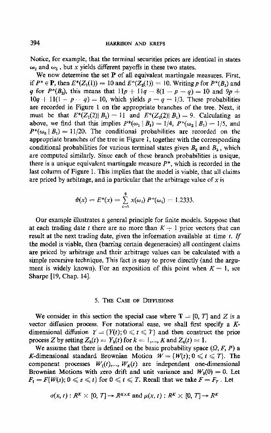
Consider the numerical example portrayed in Figure 1. There are nine states of the world, denoted o1 ,..., q, , and the trading dates are T = (0, 1,2}. We take Fl to be the field generated by the partition with cells B1 = (wl, w2, ~31, B, = {wq, w5, us}, and B3 = {w, , w8, wB}, and F2 = F to be the field generated by the total partition of L?. In other words, investors know at time t = 1 which of the events Bi has occurred, and they know at time t = 2 the state of the world. There are three securities. Of course, Z,,(t) 5 1. The prices &(t) and Zz(t) are given in Figure 1 as the nodes of the tree, Z1(t) being the upper number and Z2(t) the lower. Thus Z,(O, q) = 10, Z,(l) oJ = 11, and Z1(2, q) = 14. We shall not specify the original probability measure P on Q except to say that P(q) > 0 for all i. (The specific probabilities are irrelevant for our purposes.)

t=o t=t t=2 state X(Wi) P’koj)

l/4 14 a I 9

113 I I

:

9 “5 E I

II/m IO 1 6

"4 '9"

a

1 II “31; 114 $1

l/2 IO 1 9

l/5 I2

I IO

l/3 6 l/5 7

a II 1 I5

3/5 ,; 1

5

0

l/l2

VI5

I II60

l/l2

!/I2

l/6

l/l5

l/l5

l/5

FIG. 1. A Finite Example

We wish to know whether this model is viable and, if so, which claims are priced by arbitrage. To be concrete, we define the contingent claim

x = @Z,(2) + Z,(2) - [14 + 2 Ej& mid+&(t), Z2(t)>l>+.

This claim represents the right to buy, at the terminal date c = 2, two shares of security 1 plus one share of security 2 at a price of 14 plus twice the lowest price achieved by either of the risky securities on any of the three trading dates. The value of the claim x(q) is shown for each state of the world w( in Figure 1. We have chosen this rather silly example to emphasize that claims may depend on the complete price histories of the primitive securities.

394 HARRISON AND KRJZPS

Notice, for example, that the terminal securities prices are identical in states o2 and wg , but x yields different payoffs in these two states.

We now determine the set P of all equivalent martingale measures. First, if P* E P, then E*(Z,(l)) = 10 and E*(Z,(l)) = 10. Writingp for P*(B,) and q for P*(B,), this means that 1 lp + 1 lq + 8(1 - p - q) = 10 and 9p + IOq + 1 l(1 - p - q) = 10, which yields p = q = l/3. These probabilities are recorded in Figure 1 on the appropriate branches of the tree. Next, it must be that E*(Z,(2)[ B,) = 11 and E*(Z,(2)l B,) = 9. Calculating as above, we find that this implies P*(w, I BI) = l/4, P*(o, 1 B,) = l/5, and P*(w, I B,) = 11/20. The conditional probabilities are recorded on the appropriate branches of the tree in Figure 1, together with the corresponding conditional probabilities for various terminal states given B, and B, , which are computed similarly. Since each of these branch probabilities is unique, there is a unique equivalent martingale measure P*, which is recorded in the last column of Figure 1. This implies that the model is viable, that all claims are priced by arbitrage, and in particular that the arbitrage value of x is

i;(x) = E*(x) = i x(q) P*(wi) = 1.2333. i=l

Our example illustrates a general principle for finite models. Suppose that at each trading date t there are no more than K + 1 price vectors that can result at the next trading date, given the information available at time t. If the model is viable, then (barring certain degeneracies) all contingent claims are priced by arbitrage and their arbitrage values can be calculated with a simple recursive technique. This fact is easy to prove directly (and the argument is widely known). For an exposition of this point when K = 1, see Sharpe [19, Chap. 141.

5. THE CASE OF DIFFUSIONS

We consider in this section the special case where T = [0, Tj and Z is a vector diffusion process. For notational ease, we shall first specify a K- dimensional diffusion Y = {Y(t); 0 < t < r} and then construct the price process Z by setting Zk(t) = Y*(t) for k = l,..., Kand Z,,(t) = 1.

We assume that there is defined on the basic probability space (52, F, P) a K-dimensional standard Brownian Motion W = {W(t); 0 < t < T}. The component processes W,(t),..., WK(t) are independent one-dimensional Brownian Motions with zero drift and unit variance and W,(O) = 0. Let Ft = J’{ W(s); 0 < s < t} for 0 < t < T. Recall that we take F = FT. Let

0(x, t) : RK x [O, r] + RKXK and ~(x, t) : RK x [0, T] -+ RK


be given functions, continuous in x and t. We assume that the K x K matrix 0(x, t) is nonsingular for each x and t, so that there is a unique function c@, t) satisfying

a(~, t) - 01(x, t) + p(x, t) = 0 for x E RK, t E [0, T’J (5.1)

Here 01(x, t) and ~(x, t) should be envisioned as column vectors. Let Y be a process adapted to (Ft} and satisfying the (Ito) stochastic integral equation

for k = l,..., K and 0 < t < T, where Y(0) is a constant K-vector. See G&man and Skorohod [9] for basic definitions relating to the Ito integral and stochastic integral equations. In the usual way, we express (5.2) more compactly as

Y(t) = Y(O) + jt u(W), s) dW + jt p(W), s) ds. 0 0

(5.3)

We now define the price process Z in terms of Y as explained above. As our final assumption, we suppose the existence of a continuous K-dimensional process Y* = {Y*(t); 0 < t < T} which uniquely (up to an equivalence) satisfies

Y*(t) = Y(0) + j” u(Y*(s), s) dW, 0 < t < T. (5.4) 0

This requires some further regularity (beyond simple continuity) for the function u(*, a). See Gihman and Skorohod [9, p. 401 for sufficient conditions. We define a (K + I)-dimensional process Z* by setting Z$(t) = Y$(t) for k 3 1 and Z$(t) = 1. Before presenting our main result, we state a pre- liminary proposition which is very important for subsequent interpretations. For this proposition, let C[O, Tj be the space of continuous functions from [0, T] to RK, endowed with the topology of uniform convergence. When we say that f : C[O, Tj -+ R is a measurable functional, we mean measurable with respect to the Bore1 u-field of C[O, Tj.

PROPOSITION 1. For 0 < t < T, the u-field Ft is generated by (Z(s); 0 < s < t}. Thus every contingent claim x has the form x = f (2) for some measurable functional f : CIO, T] + R.

The proof is deferred until later in this section. Proposition 1 shows that, in allowing investors to form portfolios based on the information structure {F,}, we are giving them access only .to past and present price information at each time t. Also, with our convention F = FT , every contingent claim can


be expressed as a function of the vector price history over the interval [0, a]. Claims may depend on prices in very complicated ways, however.

The following is our main result. For a column vector y, we adopt the notation y2 for y12 + 9.. + yK2.

THEOREM 3. The set P of equivalent martingale measures is non-empty if and only if

(a) Ji a2(Y(t), t) dt < co a.s.,

(b) E(pa) < co, where p = exp(Ji o(Y(t), t) dW(t) - j$ $i a”( Y(t), t) dt)

and

(c) Y* is a martingale over (Ft}.

In this case, there is a unique P* E P, its Radon-Nikodym derivative is dP*/dP = p, and the distribution of Z on (Q, F, P*) coincides with the distribution of Z* on (Sz, F, P).

Remark. A well-known sufficient condition for (c) is

See, for example, Ash and Gardner [2, p. 2151.

COROLLARY. The securities market model is viable if and only if (a)-(c) hold. In this case, each contingent claim x E X is priced by arbitrage, with arbitrage value 73(x) = E(f(Z*)) = E*(f(Z)), where x = f(Z) as in Proposition I.

Proof of Proposition 1. For the first statement, we must show that Ft equals the u-field G, generated by {Y(s); 0 < s < t}. Let

V(t) = Y(t) - Y(0) - jO’ /A( Y(s), s) ds = jO’ u( Y(s), s) dW(s)

for 0 < t < T. Observe that V is adapted to {G,}. Fix t > 0 and define

2N-1

WNW = c {@VA tnY * v%z+d - m)l n-0

for integer N, where t, = nt/2N. (Recall that u is assumed nonsingular.) Clearly wN(t) is Gt-measurable. Using the continuity of p and u, it is easy to show that WN(t) -+ W(t) a.s. as N -+ cc, so W(t) is G,-measurable. Thus Ft C Gt . It was assumed at the outset that Y is adapted to (Ft}, so Gt C Ft , and the first statement is proved. The second statement (regarding measur-


ability) is standard and will not be proved. See, for example, Chung [5, p. 2991.

Proof of Theorem 3. We denote by Q, the set of K-dimensional processes 4 = {d(t); 0 < t < T} such that &(t, 0) is jointly measurable in t and w for each component k = l,..., K, 4 is adapted to the Brownian fields {r;‘,}, and si 42(t) dt < cc a.s. Elements of 4 will be called non-anticipating functions. The stochastic integral j $(s) &3(s) is defined for integrands 4 E @. Let P* be an equivalent martingale measure with dP* = {dP. Thus 5 is strictly positive and square integrable by definition, and the process {c(t); 0 < t < T} defined by 50) = J% I Ft) is a strictly positive martingale over the Brownian fields {F,}, with c(T) = 5 and @c(t)) = E(i) = 1 for all f. Also, using Jensen’s inequality, it is easy to show that c(t) is square integrable for each t. It is shown in Section 4 of Kunita and Watanabe [ 131 that any such martingale can be represented in the form

where y E @ further satisfies SOT E(y2(t)) dt < co. Observe that c(e) is almost surely continuous by (5.5), and from this it follows that the sample path &(*, w) of the kth component process is bounded away from zero for almost every w. Define a K-dimensional non-anticipating function 4 by setting 4,&> = r&>/L’O> for k = l,..., K. It then follows from Ito’s Lemma and (5.5) that

ln(<(t)) = s’ 4(s) dW(s) - 4 s’ +2(s) ds, 0 < t < T. 0 0

In particular, we have

5 = exp [lo’ 4(s) dW(s) - 3 Ior d”(s) dj . (5.6)

In these manipulations, we have not used the fact that P* is (by assumption) an equivalent martingale measure. Using the results of Kunita and Watanabe, it has simply been shown that any strictly positive and square integrable random variable 5 can be represented in the form (5.6).

Having achieved this representation for the Radon-Nikodym derivative [, we can use the powerful theorem of Girsanov [IO] to show that the non- anticipating function b(t) in (5.6) must in fact be a( Y(t), t). Let

W*(t) = W(t) - St d(s) ds, 0 < t < T. 0

Girsanov’s Fundamental Theorem 1 says that W* is a K-dimensional


standard Brownian Motion on (Q, F, P*) where dP* = CdP and that Y satisfies the stochastic integral equation

Y(t) = Y(O) + j t u(Y(s>, s) dW*(s) + jot p*(s) ds, (5.7) 0

on (Q, F, P*), where p*(t) = p( Y(t), t) + u( Y(t), t) 4(t). Suppose for the moment that 0(x, t) is a bounded function. Then the stochastic integral on the right side of (5.7) is a martingale on (Q, F, P*). Since Y is by assumption a martingale on (.Q, F, P*), the absolutely continuous component Jp*(s) ds must also be a martingale and this is true if and only if p*(t) = 0 for almost every t. Note well, it is in this argument that we use the assumption that P* is an equivalent martingale measure. For the case of general u the same conclusion can be reached by a stopping argument, using the fact that u(., .) is bounded on bounded sets. Let b > 0 be large and let T be the first time t such that Yk(t) = fb for some k, with T = T if no such t exists. If Y is a martingale on (Q, F, P*), then the stopped process Y(t A T) is as well, and from this one can easily argue that p*(f) = 0 for 0 < t < T. But T --+ Ta.s. as b + co, so it follows that p*(t) = 0 for all t. Details of these arguments are left to the reader. Finally, observe that p*(t) = 0 if and only if d(t) = a( Y(t), t) a.s.

We have now established that < can be the Radon-Nikodym derivative of an equivalent martingale measure P* only if 5 satisfies (5.6) with 9(t) = ol(Y(t), t) for all r, which is equivalent to the requirement 5 = p. Thus P is non-empty only if p is well defined and square integrable. This means that conditions (a) and (b) of Theorem 3 are necessary for P to be nonempty.

Suppose now that (a) and (b) hold. It is well known that this implies E(p) = 1, cf. Gihman and Skorohod [9, p. 821, so p is a legitimate Radon- Nikodym derivative. With dP* = pdP, we argue exactly as above to establish that

Y(t) = Y(0) + jt u( Y(s), s) dW*(s), 0 < t < T, 0

(5.8)

on (Q, F, P*). Since Y* uniquely satisfies (5.4) on (.Q, F, P) by assumption, we conclude that Y uniquely satisfies (5.8) on (1;2, F, P*) and that its distribution coincides with that of Y* on (Q, F, P). Thus, given (a) and (b) a necessary and sufficient condition for P* to be an equivalent martingale measure is (c). This concludes the proof of Theorem 3. The corollary follows from Theorem 2 and its corollary.

Girsanov [lo] uses the term diffusion in a broader sense than is usual, allowing the parameter functions u and p to depend on both past and present values of the vector process Y. Theorem 3 can easily be extended to this larger class of processes, but one then needs quite a lot of measure theoretic


notation to make a rigorous statement of the result. (This is required to make precise the notion of a parameter value which depends on the complete process Yin a non-anticipating way.) It also is harder to state the continuity requirement for cr, but the proof need hardly be changed at all.

6. OTHER TRADING STRATEGIES

We can not defend on economic grounds our restriction to simple trading strategies, but we can offer some comments on the consequences of relaxing it. If a larger class of trading strategies is allowed, it is necessary to say what constitutes a self-financing strategy within that larger class. Assuming this is possible, the analysis in Section 3 up to the introduction of equivalent martingale measures would not change at all. One asks whether free lunches exist and, if not, one defines the set of marketed claims (denote it M’) and the associated price functional (denote it rr’). The security market model is viable if and only if there exists some # E Y such that + 1 M’ = n’, and assuming the model is viable, a claim x is priced by arbitrage if and only if #(x) is constant as $J ranges over the set {# E Y : # 1 M’ = n’}. What may no longer hold is the one-to-one correspondence between this set of functionals $ and equivalent martingale measures. Assuming no free lunches exist with the larger class of admissible trading strategies, we have M C M’ and r’ 1 M = z-. Therefore any # E Y such that # 1 M’ = n’ satisfies $ / M = VT and gives an equivalent martingale measure (by the usual correspondence). But it may be that an equivalent martingale measure gives rise to a # E Y such that $1 M’ + T/. Thus a claim will be priced by arbitrage if it has constant expectation under all equivalent martingale measures, and its arbitrage value will be that constant, but the converse may fail to hold. Of course, if it is true that

# 1 M’ = n’ for all $ E Y such that 1c, 1 M = ,r, (6.1)

then the converse does hold. Condition (6.1) simply says that the one-to-one correspondence between equivalent martingale measures and {# E y/: Y 1 M’ = 7r’} does (fortuitously) hold.

Consider, for example, the Black-Scholes model. Enlarge the set of admissible trading strategies by allowing t, , t2 ,..., t&-l to be stopping times relative to {FJ. One can show that this enlargment does not cause free lunches to appear and that (6.1) holds. Thus, with this enlarged class of trading strategies, the Black-Scholes model is viable and all claims are priced by arbitrage.

To see how things may go awry when the set of admissible trading strategies is expanded, consider again the Black-Scholes model, and now suppose the total number of trades N is allowed to be state dependent (random). Formally,


there are non-random times 0 = to < tl < ... < T and an integer valued random variable N such that e(.) changes value only at times ti ,..., tN . So that trading strategies do not anticipate the future, we add the requirement that (N > n} E .Ft, for all n. Call such trading strategies almost simple. Then define almost simple self-financing strategies and almost simple free lunches in the obvious way. The punchline is that almost simple free lunches exist. In fact there exists an almost simple self-financing trading strategy ~9 such that

8(O) * Z(0) = 0 and e(7) . Z(T) 3 1 a.s. (6.2)

This means that if agents can employ almost simple trading strategies, the Black-Scholes model is a nonsensical model of an economic equilibrium, It is worth noting that this is not due to some peculiar property of Brownian Motion. The same statement is true for the jump process model of Cox and Ross [6].

The trading strategy that accomplishes (6.2) is not very complicated. It amounts to the well known doubling strategy by which one is sure to win at roulette: Bet on red, and keep doubling your bets until red comes out. To effect this strategy, you must be able to bet a countable number of times, although you will only bet finitely many times in any particular state. If we take t, = T- T/2N, this gives us a countable number of times to bet. To effect this strategy you also must be able to keep doubling. You will only need a finite amount of wealth for any particular state w, but this amount cannot be bounded in w. In the Black-Scholes model of frictionless markets, short sales of the bond give you the necessary funds. (This may seem to the reader an abuse of the frictionless markets assumption. Certainly, this free lunch is exorcised if there is an upper limit on the amount any agent can borrow. It would be interesting to see an alternate development of this general problem that proceeds with this sort of constraint on trading strategies.)

In the seminal papers of Black and Scholes [4] and Merton [14] on option pricing for diffusion models, and in the large literature that has followed, investors are allowed to trade continuously. This continuous trading is modeled by means of Ito integrals. Denoting by e(t) the investor’s portfolio at time t, it is assumed that O(t) is a smooth function of t and the vector of current security prices Z(t). Since Z is an Ito process, the same is true of 8, and it follows that a typical trading strategy 0 is of unbounded variation in every finite interval. With such a strategy, an agent not only executes an infinite number of transactions (trades continuously), but also buys and sells infinite quantities of stock and bond in every time interval. Defining the value process V(t) = l?(t) * Z(t) as before, the definition of the Ito integral suggests that self-financing trading strategies should be defined by the restriction

V(t) = V(0) + It O(u)dZ(u), 0 < t < T. 0


This restriction is implicit in the original treatment of Black and Scholes [4] and is explicitly displayed in Merton [15]. With these definitions, do free lunches exist? If not, is the security market model viable for some reasonable class of agents? We intend to discuss these questions in a future paper.

7. EXTENSIONS

In this section we discuss a number of extensions of the model analyzed in Sections 2 through 5. We do not give rigorous treatments owing to the amount of space that would be required. We hope that the reader will see how to make our informal arguments exact.

We have assumed throughout that one of the primitive securities is riskless and has rate of interest zero. This may seem a very restrictive assumption, but in fact it is not. We must assume that one of the securities always has strictly positive price, but if this mild assumption is met, we can use the price of that security as the numeraire. Of course, in the security market model with prices so normalized, the security which is used as numeraire is riskless and has interest rate zero.

A formal statement of this runs as follows. Fix a security market model in which no security is riskless with rate of interest zero but in which one of the K + I securities, say security zero, has &,(t, w) > 0 for all t and w. Now construct a new securities market model with the same probability space (Q, F, P), trading dates T, information structure {F,}, but with price process {Z’(t)} defined by

Obviously, Z&, o) = 1. Roughly, the original model is viable if and only if the primed model is, and claim x in the original model is priced by arbitrage if and only if claim x’ = x/Z,(T) is priced by arbitrage in the primed model. Moreover, if x and x’ are priced by arbitrage in their respective models, their arbitrage values are related by #‘(x’) = &(x)/Z,(O). This is so (roughly) because 8 is a simple self-financing trading strategy in the original model if and only if it is as well in the primed model. To see this, note that if 13 trades at times t, , t, ,..., tN, then

e(t,-,) . Z(tn) = e(t,) . Z(t,J if and only if e(t,-,) . Z’(t,) = O(t,) - Z’(h).

Thus, m E 1M if and only if m’ = m/Z,,(T) E M’, and n’(m) = nfm)/Z,,(O). To make this correspondence exact, a bit of care must be taken. Passing

from the original to the primed model involves only a change in units. Thus this transition should be economically neutral. The transition should not


change the space of contingent claims, nor should it change the topology in which agents’ preferences are assumed to be continuous. That is, it should be the case that x E X if and only if x’ E X’ and x, + x in X if and only if xk --+ x’ in X’. If Z,(T) is not bounded above and away from zero, this means that we cannot take X’ = L2(Q, F, P) and the topology on X’ to be the L2- norm topology. Rather,

and

x’ E X’ if E((x’.&(~))~) < co,

x:, -+ x’ if E({(xk - x) Z,(T)}“) --f 0.

Thus to be an equivalent martingale measure in the primed model, P* must satisfy E({(dP*/dP) Zo( T)j2) < cc instead of E({dP*/dPj2) < co. Of course, when Z,,(T) does live in a bounded subinterval of (0, co), this complication can be ignored: X’ is L2(Q, F, P), the topology on X’ is the L2 norm topology, and thus dP*/dP E L2 is the proper continuity requirement for an equivalent martingale measure.

To see this applied, consider the model actually posited by Black and Scholes [4]. There are two securities, a bond with interest rate r, so that Zo(t) = exp(rt), and a stock whose price dynamics are given by

dZ,(t) = &G(t) dt + G(t) dW),

where ,u and u are constants. The fields (FJ are those generated by the Brownian motion W. Moving to the primed model, we obtain Z;(t) =: I and Z;(t) = Z1(t) exp(-rt). Thus,

dZ;(r) = (p - r) Z;(t) dt + uZ;(t) dW(t).

Applying the results of Section 5, we know that this model is viable and that all claims are priced by arbitrage. To find the arbitrage value of a particular claim, say x = (Z,(T) - a)+, transfer to the primed model, where x’ = (Z;(T) exp(rT) - u)+/exp(rT). Then

i;‘(x’) = E(emTT(Z,X(T) err - a)+)

where dZ,* = Z,X dW. Letting dZ,O = rZ,O dt + crZ,O dW, this is

G(x) = i3’(x’)/Zo(0) = 731(X’) = E(e-‘yzlO(T) - a)+),

which is the Black-Scholes formula. The reader is invited to apply this trans- formation to Merton’s model with a stochastic interest rate [ 141. There is no


problem in passing to the primed model, but the results in Section 5 do not allow us to claim that, say, European call options can be priced by arbitrage.

Our analysis has been conducted for a world where agents consume only at dates zero and T. In the usual fashion, this can be thought of as a partial equilibrium analysis of the tradeoff between consumption at these two dates, where consumption at other dates is held fixed. But to consider claims that may pay at dates before T, including claims that may pay dividends and claims that expire at random dates, it is useful to extend our analysis to include consumption at all dates. To provide details for this would take many pages, so we leave the task to the reader. But as long as units are chosen so that there is a riskless security with rate of interest zero, the basic results that we have given hold up. Roughly, the reason is as follows. Represent a contingent claim by a function x : i2 x T -+ R where x(w, t) is the total amount paid by the claim in the time interval (0, t] if the state is w. For example, if the claim pays at a rate d(w, t) until some random time T and then pays a lump sum I(w, T), we would have

x&J, t) = JyA’d(w, s) ds + Z(w, T) * l{&) f

Consider any claim x so represented and another claim x’ where x’(w, t) = 0 for all t < T and x’(w, T) = x(w, 7’). That is, x’ pays nothing until time T, at which point it pays the totaf amount paid out by x from 0 until T. Assuming the model is viable, the price of x is determined by arbitrage if and only if that of x’ is, and their arbitrage values are equal. This is because if an agent possesses the claim x, he can invest payoffs that accrue before time Tin the riskless security. As the riskless rate of interest is zero, this yields a claim that pays x(w, T) at date T, which is exactly the claim x’. On the other hand, if an agent possesses x’, he can borrow using the riskless security to produce the pattern of returns x and, at date T, x’ will provide precisely enough funds to cover his debts. Thus the claims x and x’ are worth the same amount. The theory we have developed tells us whether claims x’ have their prices determined by arbitrage and, if so, what are their arbitragevalues. There- fore this theory answers these questions for claims such as x. One can similarly answer questions about viability by considering only claims such as x’.

Dividends paid by the primitive securities can be dealt with similarly. Again we leave the details to the reader, but note that there are a number of ways to proceed. Dividends can be “instantaneously” reinvested, either in the security which issues them or in the riskless security. Alternatively, cumulative dividends may be subtracted from the claim being valued.

Consider options next. Options are financial instruments where the bearer has some discretion as to the form or timing of the payouts. We model an option as a collection of claims (xa ; (Y E -Qz}, where the bearer has the right to


specify at the outset which claim x, he will take. For example, American puts are such collections, where 01 E & indexes all stopping times relative to (Et}. (We will return to this example momentarily.) For a viable security market model, let P denote the set of equivalent martingale measures. Then for any choice of a, the claim x, is worth no less than inf& E*(x,) and no more than SUP~*,~ E*(x,). Thus the option is worth at least

and at most

When these two numbers are equal, the option’s price is determined by arbitrage, the common number being the arbitrage value. When P is a singleton, the two numbers are obviously equal, and the value of the option is sup,,dE*(x,), where E*(.) denotes expectation with respect to the single equivalent martingale measure. Note that in such cases, the choice of which strategy cy. to elect is independent of the bearer’s attitude towards risk.

An example illustrates the three extensions given above. Consider the Black-Scholes model described above (with r possibly different from zero) and the problem of valuing an American put with exercise price a and expira- tion date T. If the put is exercised using the stopping rule 7, it generates (a - Z1(7))+ at time T. If &(T) > a, rule 7 is interpreted to imply that the put is never exercised. First we transfer to a model with zero rate of interest, getting 2’ as above. In the primed model, the option exercised using T generates (a exp(--uT) - Z;(T))+ at time 7. This is equivalent to the claim which generates (a exp(-rT) - Z;(T))+ at time T by the second extension. This claim has arbitrage value

E((ae-r7 - Z,*(T)>+),

where dZ,* = aZF dW, according to Section 5. Thus the put option has arbitrage value

Sup E({Qf?’ - z;(T)]+), I

where the supremum is over all stopping times T with 0 < T < T. (This is the arbitrage value in both the original and the primed model, as Z,,(O) = 1.) The valuation of this put is reduced to an optimal stopping problem, to which one may apply the methods of potential theory.

It is quite simple to extend beyond our restriction of X to square integrable claims and our use of the L2 norm topology. In Section 2, we only used the facts that X is a real linear space of E-measurable random variable on Q and that the topology on X is linear, Hausdorff and locally convex. (Also, it is necessary that if x E X and x’ is a random variable such that P(x = x’) = 1,


then x’ is identzjied with x as one element of X.) For any real linear space of F-measurable random variables on Sz topologized in a manner that meets these requirements, Theorem 1 is proven exactly as above. See [12] for further extensions and refinements of this.

In establishing the correspondence between # E Y such that + 1 M = rr and equivalent martingale measures (Theorem 2) we made use of the Riesz Representation Theorem. That is, $I is a continuous linear functional on X if and only if #(x) = E@ x ) f or some p E L2(Q, F, P). This told us that given a continuous linear functional #, defining P*(B) = #(lB) created a (a-additive) measure absolutely continuous with respect to P and satisfying dP*/ dP E L2. Conversely, given a probability measure P* absolutely continuous with respect to P and satisfying dP*/dP E L2, defining Z&X) = E*(x) for x E X creates a continuous linear functional on X. Suppose therefore, that we fix p E [ 1, co] and take X = Lp(!2, F, P), topologized so that Z,!I is a continuous linear functional on X if and only if #(x) = E(px) for some p E LQ@, F, P), where q-l + p-l = 1. For example, if p < co, the topology on X can be the standard L” norm topology. If p = co, the topology on X can be the L1-Mackey topology. We would need to assume that Z,(t) E X for all k and t, and we would need to change the definition of an equivalent martingale measure to read that dP*/dP E LQ. (In order to take needed conditional expectations, we would also need to require of a simple trading strategy 0 that O,(t) Z,(t) E X for all k and t.) With these changes, the development could proceed exactIy as in Section 3.

In applying this to the case of diffusions, difficulties do arise. Our use of Kunita and Watanabe [13] does require require that p E L2. So we only know conditions under which there is a unique equivalent martingale measure P* such that dP*/dP E L2. If, using the terminology of the above paragraph, we chose a p < 2, then the requirement would change to dP*/dP E LQ where q > 2. This is more stringent than dP*/dP E L2, so the conditions given in Theorem 3 establish that there is at most a single equivalent ‘martingale measure. If that measure does satisfy dP*ldP E LQ, then the model is viable and all claims are priced by arbitrage. If that measure does not satisfy dP*/dP E Lg, then the model is not viable. For example, consider the Black- Scholes model for p + 02/2 # 0. The Radon-Nikodym derivative dP*/dP can be explicitly computed, and it does not satisfy dP*/dP G L”. Thus if p = 1, the Black-Scholes model is not a viable model of economic equilibrium.

On the other hand, if p > 2, then the requirement becomes dP*/dP E LQ for q < 2. This is less stringent. Although Theorem 3 establishes the viability of a class of models (for p > 2), it does not show that the price of every contingent claim is determined by arbitrage. To do that, we would need to sharpen the Kunita-Watanabe result, and we can only conjecture that this is possible.


8. CONCLUDING REMARKS

The basic question addressed in this paper is the following. What contingent claims are “spanned” by a given set of marketed securities? To the best of our knowledge, this question first appears in the Economics literature in the classic paper by Arrow [l]. Other, more recent references include Friesen [7], Ross [16], Stiglitz [20], and the Bell Journal Symposium on the Optimality of Capital Markets [3]. The papers of Garman [8], Ross [17], and Rubinstein [18] all contain arguments similar in spirit to ours, using linear functionals to value claims whose price is determined by arbitrage.

Except for the papers of Black and Scholes [4] and Merton [14], the greatest single stimulus for the work reported here was the paper by Cox and Ross [6]. Cox and Ross provide the following key observation. If a claim is priced by arbitrage in a world with one stock and one bond, then its value can be found by first modifying the model so that the stock earns at the riskless rate, and then computing the expected value of the claim. They analyze two examples, and in each case they determine the correct modifica- tion by the follo,wing procedure. First, using the technique of Black and Scholes, they derive an analytical expression (differential or differential- difference equation) that the value of the claim must satisfy. Having observed that one model parameter does not appear in this relationship, they then adjust the value of that parameter (only) so that the stock earns at the riskless rate. Their first example is the diffusion model of Black and Scholes, where the free parameter is the drift rate of the stock price process. In their second example, the stock price pricess Y satisfies

Y(t) = y(o) + jot al’(s) dN(s) - Jot b Y(s) ds, (8.1)

where N = {N(t); 0 < t < T3 is a Poisson process with jump rate h, and a and b are specified positive constants. It is found that the free parameter is X, and that h* = b/a causes Y to earn at the riskless rate (zero).

For the Black-Scholes model, we have displayed in Section 6 the Radon- Nikodym derivative of the unique equivalent martingale measure P* under which the stock earns at the riskless rate. Substitution of P* for P is equivalent to the drift rate adjustment of Cox and Ross. For the jump process model (8.1), there also exists a unique equivalent martingale measure P*, and substitution of P* for P accomplishes the jump rate adjustment of Cox and Ross (without affecting the parameters a and b). Furthermore, it is possible to explicitly compute the Radon-Nikodym derivative of P* with respect to P. We leave to the reader the (relatively difficulty) task of computing dP*/dP and proving that P* is in fact the unique equivalent martingale measure.

The careful reader may be troubled by this comparison of Cox and Ross


with our results, because Cox and Ross state that arbitrage is independent of preferences, whereas in our treatment arbitrage is crucially tied up with a particular class of agents, the class A. It is clear how these two positions are reconciled. When Cox and Ross construct the preferences of the risk neutral agent who gives the arbitrage value of claims, they are constructing an equivalent martingale measure. In both their examples, the preferences/ measure constructed preserve the null sets of the original measure and are continuous in the sense we require. That is, their risk neutral agent is a member of our class A, as he must be.

ACKNOWLEDGMENTS

Conversations with Paul Milgrom stimulated a substantial revision of this paper, including a reformulation of the problem under discussion. We are pleased to acknowledge his very significant con$ibutions. We also benefited from conversations with James Hoag, Krishna Ramaswamy, William Sharpe, Robert Wilson, and especially George Feiger and Bertrand Jacquillat. This work was supported by a grant from the Atlantic Richfield Foundation to the Graduate School of Business, Stanford University, by National Science Foundation Grant SOC77-07741 A01 at the Institute for Mathematical Studies in the Social Sciences, Stanford University, by the Mellon Foundation, by the Churchill Founda- tion, and by the Social Science Research Council of the U.K.

REFERENCES

1. K. ARROW, The role of securities in the optimal allocation of risk-bearing, Reu. Econ. Stud. 31 (1964), 91-96.

2. R. Am AM) M. GARDNER, “Topics in Stochastic Processes,” Academic Press, New York, 1975.

3. BeZI J. Econ. Mmug. Sk., Symposium on the Optimality of Competitive Capital Markets, 5 (1974); H. LELAND, Production theory and the stock market, 125-144; R. MERTON AND M. SUBRAKMANYAM, The optimality of a competitive stock market, 145-170; S. EKERN AND R. W~SON, On the theory of the firm in an economy with incomplete markets, 171-180; R. RADNER, A note on unanimity of stockholders’ preferences among alternative production plans: A reformulation of the Ekern-Wilson model, 181-186.

4. F. BLACK AND M. SCHOLES, The pricing of options and corporate liabilities, J. PO/it. Econ. 81 (1973), 637-659.

5. K. CHUNG, “A Course in Probability Theory,” 2nd ed. Academic Press, New York, 1974.

6. J. Cox AND S. Ross, The valuation of options for alternative stochastic processes, J. Financial Econ. 3 (1976), 145-166.

7. P. FRIESEN, A Reinterpretation of the Equilibrium Theory of Arrow and Debreu in Terms of Financial Markets, Stanford University Institute for Mathematical Studies in the Social Sciences Technical Report No. 126, 1974.

8. M. GARMAN, A General Theory of Asset Valuation under Diffusion State Processes, University of California, Berkeley, Research Program in Finance Working Paper No. 50, 1976.

64212o/3-9


9. I. GIHMAN AND A. SKOROHOD, “Stochastic Differential Equations,” Springer-Verlag, New York, 1972.

10. I. GIRSANOV, On transforming a certain class of stochastic processes by absolutely continuous substitution of measures, Theor. Probability Appl. 5 (1960), 285-301.

11. R. HOLMES, “Geometric Functional Analysis and Its Applications,” Springer-Verlag, New York, 1975.

12. D. KREPS, Arbitrage and Equilibrium in Economics with Intinitely Many Commodities, Economic Theory Discussion Paper, Cambridge University, 1979.

13. H. KUNITA AND S. WATANABE, On square integrable martingales, Nagoya Math. J. 30 (1967), 209-245.

14. R. MERTON, Theory of rational option pricing, BeU J. Econ. Manag. Sci. 4 (1973), 141-183.

15. R. MERTON, On the pricing of contingent claims and the Modigliani-Miller theorem, J. Financial Econ. 5 (1977), 241-249.

16. S. Ross, The arbitrage theory of capital asset pricing, J. Econ. Theor. 13 (1976), 341-360. 17. S. Ross, A simple approach to the valuation of risky streams, J. Business 51 (1978),

453475. 18. M. RUBINSTEIN, The valuation of uncertain income streams and the pricing of options,

Bell J. Econ. 2 (1976), 407-425. *

19. W. SHARPE, “Investments,” Prentice-Hall, Englewood Cliffs, N.J., 1978. 20. J. STIGLITZ, On the optimality of the stock market allocation of investment, Quart.

J. Econ. 86 (1972), 25-60.

JOURNAL OF ECONOMIC THEORY 20, 381-408 (1979) - SFU.cakkasa/HarrisonKreps_79.pdf · JOURNAL OF...

Documents

Transcript of JOURNAL OF ECONOMIC THEORY 20, 381-408 (1979) - SFU.cakkasa/HarrisonKreps_79.pdf · JOURNAL OF...