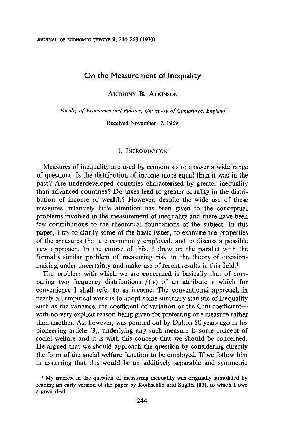
JOURNAL OF ECONOMIC THEORY 2, 244-263 (1970)

On the Measurement of Inequality

ANTHONY B. ATKINSON

Faculty of Economics and Politics, University of Cambridge, England

Received November 17, 1969

1. INTRODUCTION

Measures of inequality are used by economists to answer a wide range of questions. Is the distribution of income more equal than it was in the past? Are underdeveloped countries characterised by greater inequality than advanced countries ? Do taxes lead to greater equality in the distri- bution of income or wealth? However, despite the wide use of these measures, relatively little attention has been given to the conceptual problems involved in the measurement of inequality and there have been few contributions to the theoretical foundations of the subject. In this paper, I try to clarify some of the basic issues, to examine the properties of the measures that are commonly employed, and to discuss a possible new approach. In the course of this, I draw on the parallel with the formally similar problem of measuring risk in the theory of decision- making under uncertainty and make use of recent results in this fie1d.l

The problem with which we are concerned is basically that of com- paring two frequency distributions f(u) of an attribute y which for convenience I shall refer to as income. The conventional approach in nearly all empirical work is to adopt some summary statistic of inequality such as the variance, the coefficient of variation or the Gini coefficient- with no very explicit reason being given for preferring one measure rather than another. As, however, was pointed out by Dalton 50 years ago in his pioneering article [3], underlying any such measure is some concept of social welfare and it is with this concept that we should be concerned. He argued that we should approach the question by considering directly the form of the social welfare function to be employed. If we follow him in assuming that this would be an additively separable and symmetric

1 My interest in the question of measuring inequality was originally stimulated by reading an early version of the paper by Rothschild and Stiglitz [13], to which I owe a great deal.

244

MEASUREMENT OF INEQUALITY 245

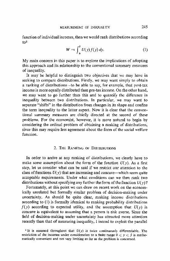
function of individual incomes, then we would rank distributions according to2

My main concern in this paper is to explore the implications of adopting this approach and its relationship to the conventional summary measures of inequality.

It may be helpful to distinguish two objectives that we may have in seeking to compare distributions. Firstly, we may want simply to obtain a ranking of distributions-to be able to say, for example, that post-tax income is more equally distributed than pre-tax income. On the other hand, we may want to go further than this and to quantify the difference in inequality between two distributions. In particular, we may want to separate “shifts” in the distribution from changes in its shape and confine the term inequality to the latter aspect. Now it is clear that the conven- tional summary measures are chiefly directed at the second of these problems. For the economist, however, it is more natural to begin by considering the ordinal problem of obtaining a ranking of distributions, since this may require less agreement about the form of the social welfare function.

2. THE RANKING OF DISTRIBUTIONS

In order to arrive at any ranking of distributions, we clearly have to make some assumption about the form of the function U(y). As a first step, let us consider what can be said if we restrict our attention to the class of functions U( JJ) that are increasing and concave-which seem quite acceptable requirements. Under what conditions can we then rank two distributions without specifying any further the form of the function U(u)?

Fortunately, at this point we can draw on recent work on the econom- ically unrelated but formally similar problem of decision-making under uncertainty. As should be quite clear, ranking income distributions according to (1) is formally identical to ranking probability distributions f(u) according to expected utility, and the assumption that U(y) is concave is equivalent to assuming that a person is risk averse. Since the field of decision-making under uncertainty has attracted more attention recently than that of measuring inequality, I intend to exploit the parallel

2 It is assumed throughout that U(y) is twice continuously differentiable. The restriction of the incomes under consideration to a finite range 0 < y 5 $ is mathe- matically convenient and not very limiting as far as the problem is concerned.

246 ATKINSON

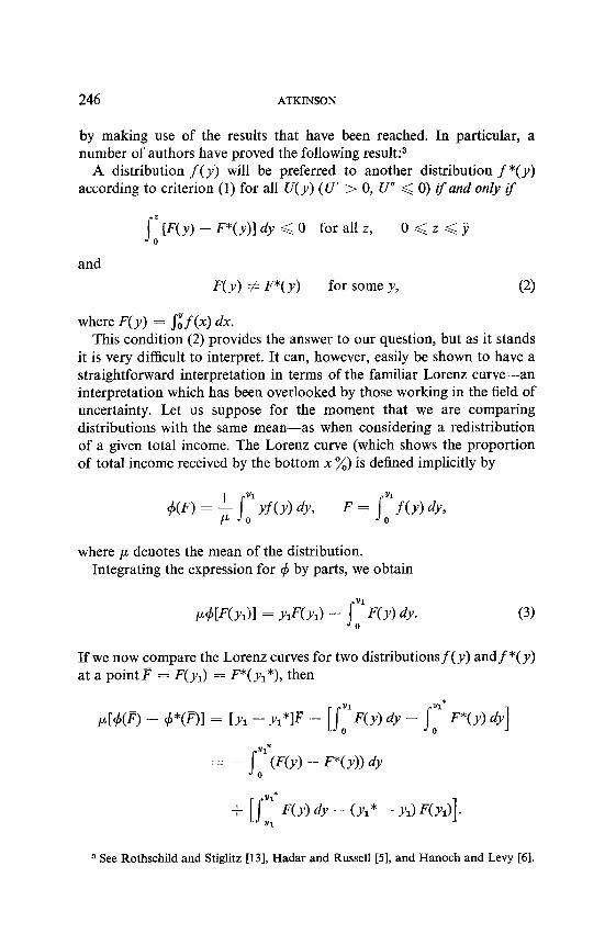
by making use of the results that have been reached. In particular, a number of authors have proved the following result:3

A distribution f(y) will be preferred to another distribution f*(y) according to criterion (1) for all U(y) (U’ > 0, U” < 0) if and only if

s

’ [F(Y) - F*(y)] dy < 0 for all z, o<z<y 0

and

F(Y) f F*(Y) for some y, (3

where F(y) = J:f(x) dx. This condition (2) provides the answer to our question, but as it stands

it is very difficult to interpret. It can, however, easily be shown to have a straightforward interpretation in terms of the familiar Lorenz curve-an interpretation which has been overlooked by those working in the field of uncertainty. Let us suppose for the moment that we are comparing distributions with the same mean-as when considering a redistribution of a given total income. The Lorenz curve (which shows the proportion of total income received by the bottom x %) is defined implicitly by

where p denotes the mean of the distribution. Integrating the expression for 4 by parts, we obtain

dH~d1 = y~F(yd - f)TyI dy. (3)

If we now compare the Lorenz curves for two distributionsf( y) and f *( y) at a point F = F(y,) = F*( yl*), then

= - ~:‘;F(Y) - F*(y)) dv

3 See Rothschild and Stiglitz [13], Hadar and Russell [5], and Hanoch and Levy [6].

MEASUREMENT OF INEQUALITY 247

Applying the first mean-value theorem, the second term is positive, so that it follows that condition (2) implies that the Lorenz curve corresponding to f(y) will lie everywhere above that corresponding to f *( y). From (3), we can also write

- s y1 [F(Y) - p*(Y)1 dy

0

= P[W{Yd - #J*(F*{YIHl - Y,[F(Yd - F*(yI)l.

But from the definition of the Lorenz curve, &(F) = Jsy dF so that

- s ‘l [F(Y) - F*(Y)] dy

0

i- PL[~(F{Y~) - +*@‘{yd)l + f;:‘, y dF* - yl(F - F*)]. 1

Again applying the first mean-value theorem to the second term, we can see that it is positive, so that if the Lorenz curve forf(y) lies above that for f*(y) for all F, then condition (2) will be satisfied. We have shown, therefore, that, when comparing distributions with the same mean, condition (2) is equivalent to the requirement that the Lorenz curves do not intersect. We can deduce that if the Lorenz curves of two distributions do not intersect, then we can judge between them without needing to agree on the form of U(y) (except that it be increasing and concave); but that if they cross, we can always find two functions that will rank them differently. If we consider distributions with different means, then condition (2) clearly implies that the mean off(y) can be no lower than that of f*(y). Conversely, if p 3 t.~* and the Lorenz curve of f(y) lies inside that off*(y) then (2) will hold.

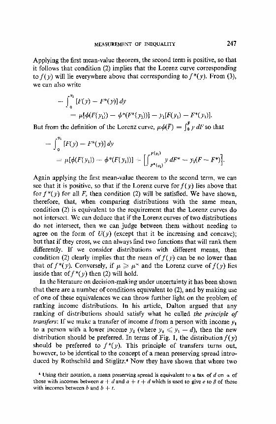
In the literature on decision-making under uncertainty it has been shown that there are a number of conditions equivalent to (2), and by making use of one of these equivalences we can throw further light on the problem of ranking income distributions. In his article, Dalton argued that any ranking of distributions should satisfy what he called the principle of transfers: If we make a transfer of income d from a person with income y1 to a person with a lower income y2 (where yZ < y1 - d), then the new distribution should be preferred. In terms of Fig. 1, the distribution f( y) should be preferred to f*(y). This principle of transfers turns out, however, to be identical to the concept of a mean preserving spread intro- duced by Rothschild and Stiglitz.4 Now they have shown that where two

4 Using their notation, a mean preserving spread is equivalent to a tax of d on OL of those with incomes between a + d and a + I + d which is used to give e to fi of those with incomes between b and b + t.

248 ATKINSON

1 lncomey

FIG. 1. The principle of transfers.

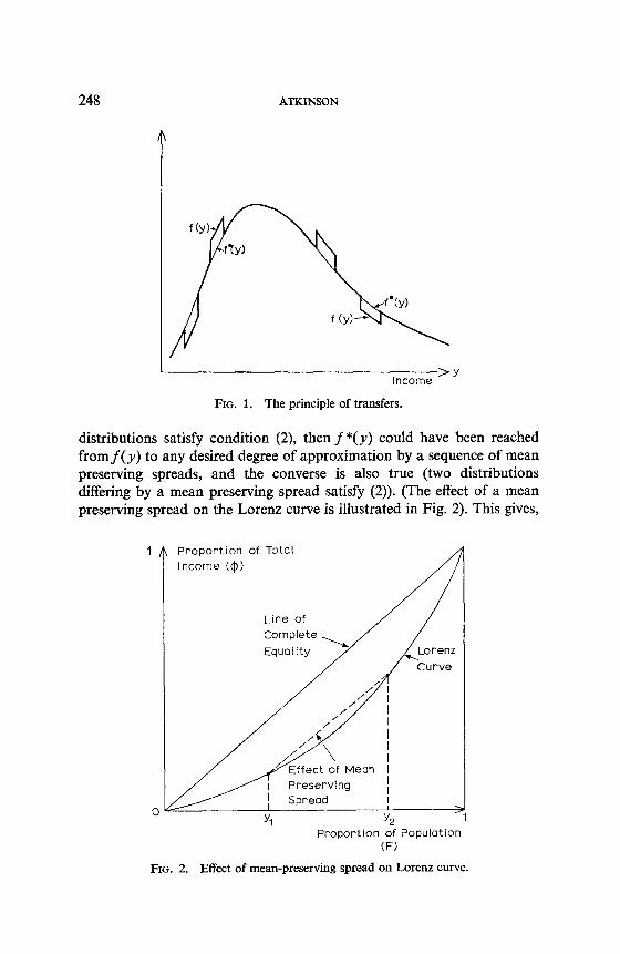
distributions satisfy condition (2), then f*(v) could have been reached from f (u) to any desired degree of approximation by a sequence of mean preserving spreads, and the converse is also true (two distributions differing by a mean preserving spread satisfy (2)). (The effect of a mean preserving spread on the Lorenz curve is illustrated in Fig. 2). This gives,

1 Proportion of Total

Income ($1

Line of

Proportion of Population (F)

FIG. 2. Effect of mean-preserving spread on Lorenz curve.

MEASUREMENT OF INEQUALITY 249

therefore, an alternative interpretation of condition (2): a necessary and sufficient condition for us to be able to rank two distributions independently of the utility function (other than that it be increasing and concave) is that one can be obtained from the other by redistributing income from the richer to the poorer. That the concavity of U(y) is sufficient to guarantee that the principle of transfers holds is hardly surprising; however, it is not so obvious that this is the widest class of distributions that can be ranked without any further restriction of the form of WY>.

3. COMPLETE RANKING AND EQUALLY DISTRIBUTED EQUIVALENT INCOME

The results of the previous section demonstrate that we cannot obtain a complete ordering of distributions according to (1) unless we are prepared to specify more precisely the form of the function U(y). It is in fact clear that for a complete ranking we need to specify U(v) up to a (monotonic) linear transformation. In the rest of the paper, I consider the implications of alternative social welfare functions and their relation to the summary measures that are commonly used.

The specification of the function U(y) will provide a ranking of all distributions; it will also, however, allow us to meet the second objective of quantifying the degree of inequality. Dalton, for example, suggested that we should use as a measure of inequality the ratio of the actual level of social welfare to that which would be achieved if income were equally distributed:

Jf WY)f(Y) dY U(P) *

(4)

This normalisation is not, however, invariant with respect to linear transformations of the function U(y); for example, in the case of the logarithmic utility function, Dalton’s measure is5

JZ WY)f(Y) dY + c

hh-4 + c ’

the value of which clearly depends on c. So that although two people might agree that the social welfare function should be logarithmic-and hence agree on the ranking of distributions-their measures of inequality

6 See Ref. [3], p. 350.

250 ATKINSON

would only coincide if they agreed also about the value of c. For this reason, the measure suggested by Dalton is not very useful.”

We can, however, obtain a measure of inequality that is invariant with respect to linear transformations by introducing the concept of the equaZly distributed equivalent level of income ( yEna) or the level of income per head which if equally distributed would give the same level of social welfare as the present distribution’, that is,

WYEDE)/~~(Y)~~ = 1: V~>f(~)dy. 0

We can then define as our new measure of inequality

or 1 minus the ratio of the equally distributed equivalent level of income to the mean of the actual distribution. If Z falls, then the distribution has become more equal-we would require a higher level of equally distributed income (relative to the mean) to achieve the same level of social welfare as the actual distribution. The measure Z has, of course, the convenient property of lying between 0 (complete equality) and 1 (complete inequality). Moreover, this new measure has considerable intuitive appeal. If Z = 0.3, for example, it allows us to say that if incomes were equally distributed, then we should need only 70 ‘A of the present national income to achieve the same level of social welfare (according to the particular social welfare function). Or we could say that a certain plan for redistributing income would raise social welfare by an amount equivalent to an increase of 5 % in equally distributed income. This facilitates comparison of the gains from redistribution with the costs that it might impose-such as any disincentive effect of income taxation-and with the benefits from alter- native economic measures. Finally, it should be clear that the concept of

6 Dalton’s approach has been applied by Wedgwood [15], who calculated that in the case of the logarithmic function the level of welfare associated with the actual distribution of income in Great Britain in 1919-1920 was only 77 % of what it would have been had income been equally distributed.

A similar approach has been adopted by Aigner and Heins [l]. For the reason described in the text, however, the particular numerical values calculated by these authors have no meaning.

’ This line of approach was suggested to me by discussions with David Newbery. It also resembles the work of Mirrlees and Stern in a quite different context [9].

MEASUREMENT OF INEQUALITY 251

equally distributed equivalent income is closely related to that of a risk premium or certainty equivalent in the theory of decision-making under uncertainty. YEr,n is simply the analogue of the certainty equivalent and I is equal to the proportional risk premium as defined by Pratt [I 11.8 This parallel conveniently allows us once more to borrow results.

Before examining the implications of specific measures, it may be helpful to discuss some of the general properties that we should like such measures to possess. In particular, I should like to consider the relationship between inequality per se and general shifts in the distribution. Nearly all the measures conventionally used are concerned to measure inequality independently of the mean level of incomes; so that if the distribution of income in country A is simply a scaled-up version of that in country B, fA( v) = fB(Oy), then we should regard them as characterised by the same degree of inequality. Now suppose that we were to require that the equally distributed measure I were invariant with respect to such propor- tional shifts, so that we could consider the degree of inequality indepen- dently of the mean level of incomes. Then by applying the results of Pratt [l 11, Arrow [2], and others, we can see that this requirement (which may be referred to as constant (relative) inequality-aversion) implies that U(y) has the form

U(y) = A + I?&, Efl

and (5) U(Y) = 1%. (Y>, E= 1,

where we require E >, 0 for concavity. On the other hand, it might quite reasonably be argued that as the general level of incomes rises we are more concerned about inequality-that I should rise with proportional additions to incomes. In other words, the social welfare function should exhibit increasing (relative) inequality-aversion. In that event, the measure of inequality I can only be interpreted with reference to the mean of the distribution.

The previous paragraph was concerned with the effect of equal propor- tional additions to income; we may also consider the effect of equal absolute additions to incomes (denoted by 8). We can then define a measure of absolute inequality-aversion (which is again parallel to the measure of

8 The proportional risk premium is defined as the amount T* such that a person with initial wealth W would be indifferent between accepting a risk Wz (where z is a random variable) and receiving the non-random amount E( Wz) - Wm*. In the

present case, W = p and z = (y - p)/p.

252 ATKINSON

risk-aversion in the theory of uncertainty):Q Absolute inequality-aversion is increasing/constant/decreasing according as

&r,E/LV9 is less than/equal to/greater than 1.

It has been argued by a number of writers that equal absolute additions to all incomes should reduce inequality; if one looks at the effect on 1, this has the sign of

(1 -I)-%.

From this we can see that I may fall with equal absolute additions to income even if absolute inequality-aversion is increasing.

4. SPECIFIC MEASURES OF INEQUALITY

So far I have discussed general principles without considering specific measures of inequality. In this section, I examine some of the implications of different measures, beginning with the conventional summary statistics.

The Conventional Summary Measures

The measures most commonly used in empirical work include the following: (a) the variance, V2; (b)- the coefficient of variation, V/p; (c) the relative mean deviation, Ji 1 y/p - 1 If(y) dy; (d) the Gini coefficient, 1/2p-J: [ yF( y) - &( y)]f( y) dy; (e) the standard deviation of logarithms, .fi UogWcLA”f(v> dv.

The implications of the earlier discussion for the use of these summary measures can be seen as follows. If we consider distributions with the same mean and apply one of the measures (a)-(d), then we are guaranteed to arrive at the same ranking as with an arbitrary concave social welfare function if and only if condition (2) is satisfied.lO For example, if con-

9 This definition can be seen to be parallel to that for the uncertainty case since JJEDE is equal to p - =, where n is the absolrrte risk premium (for an absolute gamble y - /L and initial assets p).

lo In the case of the variance, this follows directly-see [13]. For the other measures, the restriction to distributions with the same mean is important. In the case of measures (b) and (c), we can write them in the form

where V is convex in y (N.B. the integral is minimised to give the least inequality). While the Gini coefficient cannot in general be written in this form (as shown by the example of Newbery [lo]), the same result can be shown to hold.

MEASUREMENT OF INEQUALITY 253

dition (2) holds (and the distributions have the same mean), then the Gini coefficient will give the same ranking as any concave social welfare function (this is clearly the case since it represents the area between the Lorenz curve and the line of complete equality); but if (2) does not hold, we can always find a function U(y) such that the distribution with the higher Gini coefficient is preferred. With these measures it follows, therefore, that they will give the same ranking of distributions satisfying (2), but where this condition is not met, they may give conflicting results.ll Dalton suggested that “in most practical cases” the measures would in fact give the same ranking, so that we could rely on the “corroboration of several.” However, as the work of Yntema [16], Ranadive [12] and others has demonstrated, this expectation is not borne out and in practice the measures give quite different rankings. Much of the early literature was in fact concerned with the problem of choosing between the different summary measures, and such properties were discussed as ease of computation, ease of inter- pretation, the range of variation, and whether they required information about the entire distribution. However, as I have emphasised earlier, the central issue clearly concerns the underlying assumption about the form of the social welfare function that is implicit in the choice of a particular summary measure. It is, therefore, on this aspect that I shall concentrate here.

The first issue is one discussed in the previous section-the dependence of the measures on the mean income. With the exception of the variance, all the measures listed above are defined relative to the mean, so that they are unaffected by equal proportional increases in all incomes. In the case of the variance, we know from the theory of uncertainty that ranking distributions according to mean and variance is equivalent to assuming that U(y) is quadratic, and that this in turn implies increasing relative and absolute inequality-aversion. As argued earlier, increasing relative inequality-aversion may be a quite acceptable property of the social welfare function. Increasing absolute inequality-aversion, however, may be less reasonable: It means that equal absolute increases in all incomes cause the equally distributed equivalent income to rise by less than the same amount. While the objections to this property are less strong than the corresponding objections in the uncertainty case, it may be grounds for rejecting the quadratic. In any event, it is the mean independent measures (b)-(e) that have received most attention, and for this reason I shall concentrate on them here.

I1 The relationship between cases where the conventional measures give conflicting rankings and the crossing of the Lorenz curves was suggested by Ranadive [12]; the results given in Section 2 provide a proof of this.

254 ATKINSON

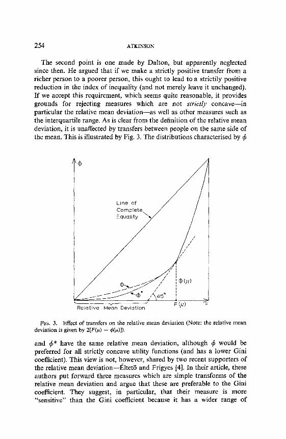
The second point is one made by Dalton, but apparently neglected since then. He argued that if we make a strictly positive transfer from a richer person to a poorer person, this ought to lead to a strictily positive reduction in the index of inequality (and not merely leave it unchanged). If we accept this requirement, which seems quite reasonable, it provides grounds for rejecting measures which are not strictly concave-in particular the relative mean deviation-as well as other measures such as the interquartile range. As is clear from the definition of the relative mean deviation, it is unaffected by transfers between people on the same side of the mean. This is illustrated by Fig. 3. The distributions characterised by 4

4

Line of

Relative Mean Deviation 3

FIG. 3. Effect of transfers on the relative mean deviation (Note: the relative mean deviation is given by 2[F(p) - &)I).

and 4* have the same relative mean deviation, although 4 would be preferred for all strictly concave utility functions (and has a lower Gini coefficient). This view is not, however, shared by two recent supporters of the relative mean deviation-altetii and Frigyes [4]. In their article, these authors put forward three measures which are simple transforms of the relative mean deviation and argue that these are preferable to the Gini coefficient. They suggest, in particular, that their measure is more “sensitive” than the Gini coefficient because it has a wider range of

MEASUREMENT OF INEQUALITY 255

variation, but ignore the fact that it is completely insensitive to transfers between people on the same side of the mean.12

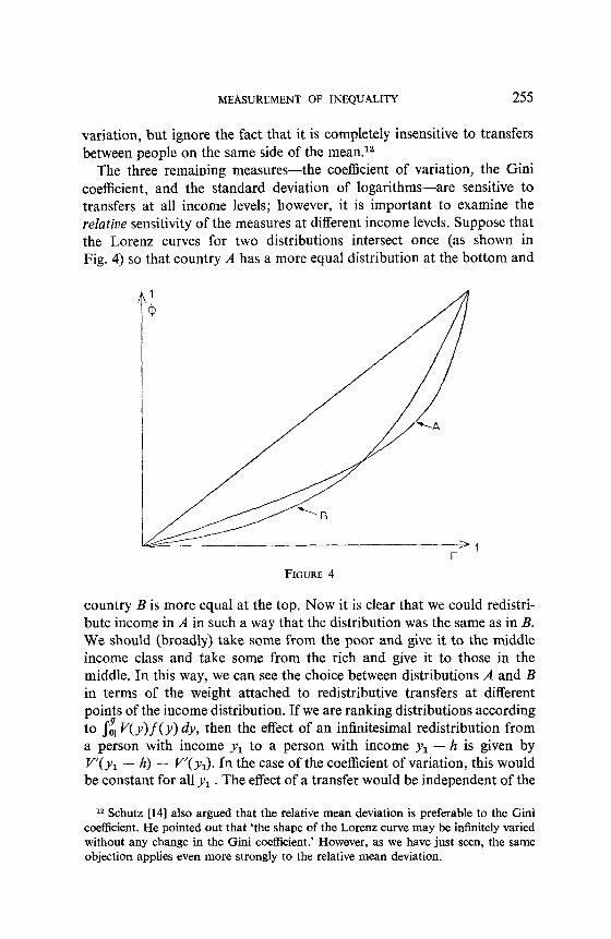
The three remaining measures-the coefficient of variation, the Gini coefficient, and the standard deviation of logarithms-are sensitive to transfers at all income levels; however, it is important to examine the relative sensitivity of the measures at different income levels. Suppose that the Lorenz curves for two distributions intersect once (as shown in Fig. 4) so that country A has a more equal distribution at the bottom and

'I F

FIGURE 4

country B is more equal at the top. Now it is clear that we could redistri- bute income in A in such a way that the distribution was the same as in B. We should (broadly) take some from the poor and give it to the middle income class and take some from the rich and give it to those in the middle. In this way, we can see the choice between distributions A and B in terms of the weight attached to redistributive transfers at different points of the income distribution. If we are ranking distributions according to $, V( y)f( y) dy, then the effect of an infinitesimal redistribution from a person with income y1 to a person with income y1 - h is given by V’( y1 - h) - V’( yJ. In the case of the coefficient of variation, this would be constant for all y1 . The effect of a transfer would be independent of the

I2 Schutz [14] also argued that the relative mean deviation is preferable to the Gini coefficient. He pointed out that ‘the shape of the Lorenz curve may be infinitely varied without any change in the Gini coefficient.’ However, as we have just seen, the same objection applies even more strongly to the relative mean deviation.

256 ATKINSON

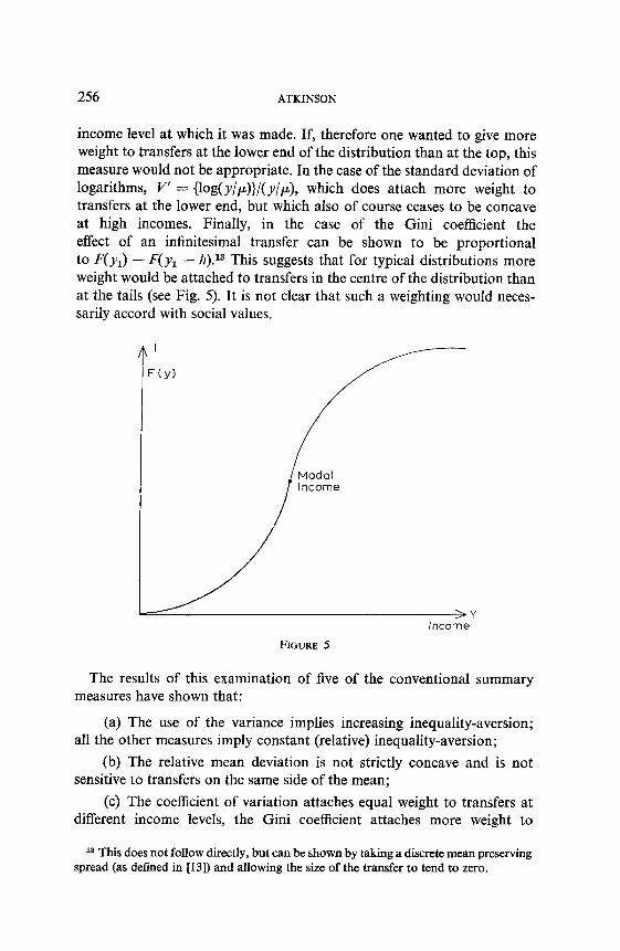
income level at which it was made. If, therefore one wanted to give more weight to transfers at the lower end of the distribution than at the top, this measure would not be appropriate. In the case of the standard deviation of logarithms, v’ = {log(y/p)}/(y/p), which does attach more weight to transfers at the lower end, but which also of course ceases to be concave at high incomes. Finally, in the case of the Gini coefficient the effect of an infinitesimal transfer can be shown to be proportional to J’(:(ur) - F(y, - h).13 This suggests that for typical distributions more weight would be attached to transfers in the centre of the distribution than at the tails (see Fig. 5). It is not clear that such a weighting would neces- sarily accord with social values.

A’ F(y)

FIGURE 5

>v Income

The results of this examination of five of the conventional summary measures have shown that:

(a) The use of the variance implies increasing inequality-aversion; all the other measures imply constant (relative) inequality-aversion;

(b) The relative mean deviation is not strictly concave and is not sensitive to transfers on the same side of the mean;

(c) The coefficient of variation attaches equal weight to transfers at different income levels, the Gini coefficient attaches more weight to

I8 This does not follow directly, but can be shown by taking a discrete mean preserving spread (as defined in [13]) and allowing the size of the transfer to tend to zero.

MEASUREMENT OF INEQUALITY 257

transfers affecting middle income classes and the standard deviation weights transfers at the lower end more heavily.

The Social Welfare Function Approach

In the previous section, I examined the implicit assumptions about the form of the social welfare function embodied in the conventional summary measures and suggested that a number of these assumptions were unlikely to command wide support. In any case, it seems more reasonable to approach the question directly by considering the social welfare function that we should like to employ rather than indirectly through these summary statistical measures. While there is undoubtedly a wide range of dis- agreement about the form that the social welfare function should take, this direct approach allows us to reject at once those that attract no supporters, and also serves to emphasise that any measure of inequality involves judgements about social welfare.

The social welfare function considered here is assumed to be of the form (1) that we have been discussing throughout; that is, it is symmetric and additively separable in individual incomes-although this is, of course, restrictive. Now we have seen that nearly all the conventional measures are defined relative to the mean of the distribution, so that they are invariant with respect to proportional shifts. If we want the equally distributed equivalent measure to have this property, then this restricts us still further to the class of homothetic functions (5), which in the case of discrete distributions imply a measure

1 = 1 - [T (yf(yi)]l’(l-e).

In this case, the question is narrowed to one of choosing E, which is clearly a measure of the degree of inequality-aversion-or the relative sensitivity to transfers at different income levels. As E rises, we attach more weight to transfers at the lower end of the distribution and less weight to transfers at the top. The limiting case at one extreme is E -+ 00 giving the function mini {vi} which only takes account of transfers to the very lowest income group (and is therefore not strictly concave); at the other extreme we have E = 0 giving the linear utility function which ranks distributions solely according to total income.l*

I4 It should be noted that the measure is readily decomposable if it is desired to measure the contribution of inequality within and inequality between subgroups of the population.

258 ATKINSON

5. AN ILLUSTRATION

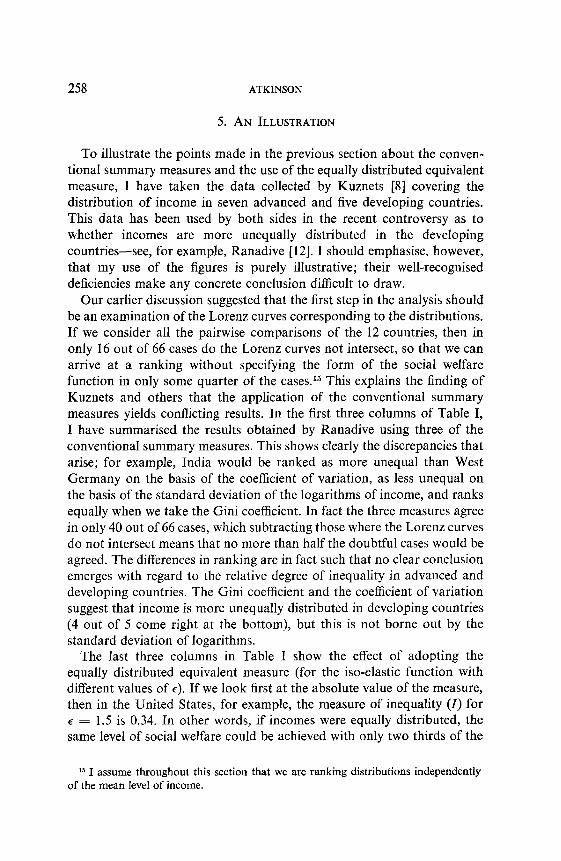
To illustrate the points made in the previous section about the conven- tional summary measures and the use of the equally distributed equivalent measure, I have taken the data collected by Kuznets [8] covering the distribution of income in seven advanced and five developing countries. This data has been used by both sides in the recent controversy as to whether incomes are more unequally distributed in the developing countries-see, for example, Ranadive [12]. I should emphasise, however, that my use of the figures is purely illustrative; their well-recognised deficiencies make any concrete conclusion difficult to draw.

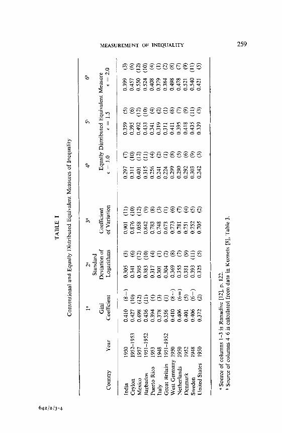
Our earlier discussion suggested that the first step in the analysis should be an examination of the Lorenz curves corresponding to the distributions. If we consider all the pairwise comparisons of the 12 countries, then in only 16 out of 66 cases do the Lorenz curves not intersect, so that we can arrive at a ranking without specifying the form of the social welfare function in only some quarter of the cases.15 This explains the finding of Kuznets and others that the application of the conventional summary measures yields conflicting results. In the first three columns of Table I, I have summarised the results obtained by Ranadive using three of the conventional summary measures. This shows clearly the discrepancies that arise; for example, India would be ranked as more unequal than West Germany on the basis of the coefficient of variation, as less unequal on the basis of the standard deviation of the logarithms of income, and ranks equally when we take the Gini coefficient. In fact the three measures agree in only 40 out of 66 cases, which subtracting those where the Lorenz curves do not intersect means that no more than half the doubtful cases would be agreed. The differences in ranking are in fact such that no clear conclusion emerges with regard to the relative degree of inequality in advanced and developing countries. The Gini coefficient and the coefficient of variation suggest that income is more unequally distributed in developing countries (4 out of 5 come right at the bottom), but this is not borne out by the standard deviation of logarithms.

The last three columns in Table I show the effect of adopting the equally distributed equivalent measure (for the iso-elastic function with different values of l ). If we look first at the absolute value of the measure, then in the United States, for example, the measure of inequality (1) for E = 1.5 is 0.34. In other words, if incomes were equally distributed, the same level of social welfare could be achieved with only two thirds of the

I5 I assume throughout this section that we are ranking distributions independently of the mean level of income.

TABL

E I

Con

vent

iona

l an

d Eq

ually

D

istri

bute

d Eq

uiva

lent

M

easu

res

of I

nequ

ality

Cou

ntry

Ye

ar

1”

Gin

i C

oeffi

cien

t

2”

Stan

dard

D

evia

tion

of

Loga

rithm

s

3”

46

5b

6b

Coe

ffici

ent

Equa

lly

Dis

tribu

ted

Equi

vale

nt

Mea

sure

of

Var

iatio

n E

= 1.

0 E

= 1.

5 E

= 2.

0

Indi

a 19

50

Cey

lon

1952

-195

3 M

exico

19

57

Barb

ados

19

51-1

952

Puer

to

Ric

o 19

53

Italy

19

48

Gre

at

Brita

in

1951

-195

2 W

est

Ger

man

y 19

50

Net

herla

nds

1950

D

enm

ark

1952

Sw

eden

19

48

Uni

ted

Stat

es

1950

0.41

0 (8

=)

0.42

7 (1

0)

0.49

8 (1

2)

0.43

6 (1

1)

0.39

4 (4

) 0.

378

(3)

0.35

6 (I)

0.

410

(8=)

0.

406

(6=)

0.

401

(5)

0.40

6 (6

=)

0.37

2 (2

)

0.30

5 (3

) 0.

341

(6)

0.39

5 (1

2)

0.38

3 (1

0)

0.31

7 (4

) 0.

301

(1)

0.30

4 (2

) 0.

369

(8)

0.35

5 (7

) 0.

381

(9)

0.39

3 (1

1)

0.32

5 (5

)

0.90

1 (1

1)

0.87

6 (1

0)

1.05

8 (1

2)

0.84

2 (9

) 0.

783

(8)

0.74

8 (3

) 0.

673

(1)

0.77

3 (6

) 0.

781

(7)

0.75

1 (4

) 0.

752

(5)

0.70

5 (2

)

0.29

7 (7

) 0.

311

(10)

0.

401

(12)

0.

315

(11)

0.

256

(4)

0.24

1 (2

) 0.

224

(1)

0.29

9 (8

) 0.

290

(5)

0.29

2 (6

) 0.

303

(9)

0.24

2 (3

)

0.35

9 (5

) 0.

395

(6)

0.49

2 (1

2)

0.43

3 (1

0)

0.34

1 (4

) 0.

319

(2)

0.31

1 (1

) 0.

411

(8)

0.39

5 (7

) 0.

418

(9)

0.43

5 (1

1)

0.33

9 (3

)

0.39

9 (3

) 0.

457

(6)

0.55

0 (1

2)

0.52

4 (1

0)

0.40

8 (4

) 0.

379

(I)

0.38

4 (2

) 0.

498

(8)

0.47

8 (7

) 0.

521

(9)

0.54

0 (1

1)

0.42

1 (5

)

R So

urce

of

col

umns

l-3

is

Ran

adiv

e [1

2],

p. 1

22.

b So

urce

of

col

umns

4-

6 is

cal

cula

ted

from

da

ta

in K

uzne

ts

[B],

Tabl

e 3.

260 ATKINSON

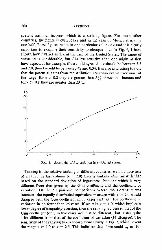
present national income-which is a striking figure. For most other countries, the figure is even lower and in the case of Mexico it is only one-half. These figures relate to one particular value of E and it is clearly important to examine their sensitivity to changes in E. In Fig. 6, I have shown how I varies with E in the case of the United States. The range of variation is considerable, but I is less sensitive than one might at first have expected; for example, if we could agree that E should be between 1.5 and 2.0, then I would lie between 0.42 and 0.34. It is also interesting to note that the potential gains from redistribution are considerable over most of the range: for E > 0.2 they are greater than 5 % of national income and for E > 0.8 they are greater than 20 7;.

E- FIG. 6. Sensitivity of Z to variation in +-United States.

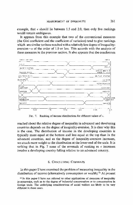
Turning to the relative ranking of different countries, we may note first of all that the last column (E = 2.0) gives a ranking identical with that based on the standard deviation of logarithms, but one which is very different from that given by the Gini coefficient and the coefficient of variation. Of the 50 pairwise comparisons where the Lorenz curves intersect, the equally distributed equivalent measure with E = 2.0 would disagree with the Gini coefficient in 17 cases and with the coefficient of variation in no fewer than 26 cases. If we take E = 1.0, which implies a lower degree of inequality-aversion, then the ranking is closer to that of the Gini coefficient (only in five cases would it be different), but is still quite a lot different from that of the coefficient of variation (14 disagree). The sensitivity of the ranking to E is shown more clearly in Fig. 7, which covers the range E = 1.0 to E = 2.5. This indicates that if we could agree, for

MEASUREMENT OF INEQUALITY 261

example, that E should lie between 1.5 and 2.0, then only five rankings would remain ambiguous.

It appears from this example that two of the conventional measures (the Gini coefficient and the coefficient of variation) tend to give rankings which are similar to those reached with a relatively low degree of inequality- aversion--E of the order of 1.0 or less. This accords with the analysis of these measures in the previous section. It also appears that the conclusions

MEXICO SWEDEN

--I 4 I.0 I.25 15 1.75 20 2-25 25

c

FIG. 7. Ranking of income distributions for different values of E.

reached about the relative degree of inequality in advanced and developing countries depends on the degree of inequality-aversion. It is clear why this is the case. The distribution of income in the developing countries is typically more equal at the bottom and less equal at the top than in the advanced countries, and as the degree of inequality-aversion increases, we attach more weight to the distribution at the lower end of the scale. It is striking that in Fig. 7 none of the reversals of ranking as E increases involve a developing country falling relative to an advanced country.

6. CONCLUDING COMMENTS

In this paper I have examined the problem of measuring inequality in the distribution of income (alternatively consumption or wealth).16 At present

I6 In this paper I have not referred to other applications of measures of inequality in economics, such as to the degree of industrial concentration or to concentration in foreign trade. The underlying considerations of social welfare are likely to be very different in these cases.

262 ATKINSON

this problem is usually approached through the use of such summary statistics as the Gini coefficient, the variance or the relative mean deviation. I have tried to argue, however, that this conventional method of approach is misleading. Firstly, the use of these measures often serves to obscure the fact that a complete ranking of distributions cannot be reached without fully specifying the form of the social welfare function. Secondly, exam- ination of the social welfare functions implicit in these measures shows that in a number of cases they have properties which are unlikely to be accept- able, and in general there are no grounds for believing that they would accord with social values. For these reasons, I hope that these conventional measures will be rejected in favour of direct consideration of the properties that we should like the social welfare function to display.

ACKNOWLEDGMENTS

I am very grateful to P. Dasgupta, G. M. Heal, A. Klevorick, D. M. G. Newbery, M. Rothschild, J. E. Stiglitz, and the referees for their comments on earlier versions of this paper, which have led to considerable improvements. After the paper was accepted for publication, I discovered that a number of the results have been proved independently in an important paper by S. Ch. Kolm [7]. However, I feel that the rather different approach adopted here may still be of interest.

REFERENCES

1. D. J. AIGNER AND A. J. HEINS, A social welfare view of the measurement of income inequality, Rev. Income Wealth 13 (March 1967).

2. K. J. ARROW, “Aspects of the Theory of Risk Bearing,” Helsinki, 1965. 3. H. DALTON, The measurement of the inequality of incomes, Econ. J. 30 (September

1920). 4. 0. I?LTETB AND E. FRIGYES, New income inequality measures as efficient tools for

causal analysis and planning, Econometrica 36 (April 1968). 5. J. HADAR AND W. R. RUSSELL, Rules for ordering uncertain prospects, Amer. Econ.

Rev. 59 (March 1969). 6. G. HANOCH AND H. LEVY, The efficiency analysis of choices involving risk, Rev.

Econ. Studies 36 (July 1969). 7. S. CH. KOLM, The optimal production of social justice, in “Public Economics,”

(J. Margolis and H. Guitton, Eds.), Macmillan, New York/London, 1969. 8. S. KUZNETS, Quantitative aspects of economic growth of nations: VIII Distribution

of income by size, Econ. Development Cultural Change 11 (January 1963). 9. J. A. MIRRLEES AND N. H. STERN, “On Fairly Good Plans,” Mimeo, 1969.

10. D. M. G. NEWBERY, A theorem on the measurement of inequality, J. Econ. Theory 2 (1970), 264.

11. J. W. PRATT, Risk aversion in the small and large, Econometrica 32 (January-April 1964).

12. K. R. RANADNE, The equality of incomes in India, Bull. Oxford Institute of Statistics 27 (May 1965).

MEASUREMENT OF INEQUALITY 263

13. M. ROTHSCHILD AND J. E. STIGLITZ, “Increasing Risk: A Definition and its Econo- mic Consequences,” Cowles Foundation Discussion Paper 275, May 27, 1969.

14. R. R. SCHUTZ, On the measurement of income inequality, Amer. Econ. Rev. 41 (March 1951).

15. J. WEDGWOOD, “The Economics of Inheritance,” Penguin Books, London, 1939. 16. D. B. YNTEMA, Measures of inequality in the personal distribution of income or

wealth, J. Amer. Statisr. Assoc. 28 (December 1933).