JOURNAL OF DIFFERENTIAL EQUATIONS, -...
16
JOURNAL OF DIFFERENTIAL EQUATIONS, 3, 15-30 (1967). Perturbation Theorems for Ordinary Differential Equations AARON STRAUSS AND JAMES A. YORKE* Department of Mathematics, University of Maryland, College Park, Maryland Received July 28, 1965 Consider the following systems of ordinary differential equations: x’ =.f(4 4, (NJ x’ =“f@, 4 + g(4 4, (P) x’ =.f(4 4 + g(c 4 + h(t), (PI) where f(t, X) is continuous, satisfies a Lipschitz condition on some semi- cylinder, f(t, 0) = 0, and x = 0 is uniform asymptotically stable for (N). Let g(t, x) and h(t) be sufficiently smooth for local existence and uniqueness. Consider the conditions (Hi): There exists r > 0 such that if 1 x 1 < Y, then 1 g(t, x)1 < y(t) for all t 3 0, where G(t) = ,:, y(s)ds+O as t-+cc. (1.1) (Hs): There exists a continuous, nonincreasing function H(t) satisfying lim H(t) = 0 t-m2 such that 1 & h(s) ds 1 < H(t,) for every 0 < t, < t < t, + 1. Then we prove: If g(t, X) satisfies (Hi) and h(t) satisfies (Ha), then there exists T,, > 0 and 6, > 0 such that if t, > T, and j x0 1 < 6, the solution F(t, t, , x0) of (PJ approaches zero as t + cg. In particular, if x = 0 is a solution of (PI), then it is uniform asymptotically stable. Furthermore, if g(t, X) = 0 and h(t) does not satisfy (Ha), then 120 solution of (PI) can approach zero as t+ co. In the casef(t, x) = Ax, where A is a constant matrix, the above results * The second author holds an NSF Co-op. Fellowship. 15
Transcript of JOURNAL OF DIFFERENTIAL EQUATIONS, -...

JOURNAL OF DIFFERENTIAL EQUATIONS, 3, 15-30 (1967).
Perturbation Theorems for Ordinary Differential Equations
AARON STRAUSS AND JAMES A. YORKE*
Department of Mathematics, University of Maryland, College Park, Maryland
Received July 28, 1965
Consider the following systems of ordinary differential equations:
x’ =.f(4 4, (NJ
x’ =“f@, 4 + g(4 4, (P)
x’ =.f(4 4 + g(c 4 + h(t), (PI)
where f(t, X) is continuous, satisfies a Lipschitz condition on some semi- cylinder, f(t, 0) = 0, and x = 0 is uniform asymptotically stable for (N). Let g(t, x) and h(t) be sufficiently smooth for local existence and uniqueness. Consider the conditions
(Hi): There exists r > 0 such that if 1 x 1 < Y, then 1 g(t, x)1 < y(t) for all t 3 0, where
G(t) = ,:, y(s)ds+O as t-+cc. (1.1)
(Hs): There exists a continuous, nonincreasing function H(t) satisfying
lim H(t) = 0 t-m2
such that 1 & h(s) ds 1 < H(t,) for every 0 < t, < t < t, + 1. Then we prove: If g(t, X) satisfies (Hi) and h(t) satisfies (Ha), then there exists T,, > 0 and 6, > 0 such that if t, > T, and j x0 1 < 6, the solution F(t, t, , x0) of (PJ approaches zero as t + cg. In particular, if x = 0 is a solution of (PI), then it is uniform asymptotically stable. Furthermore, if g(t, X) = 0 and h(t) does not satisfy (Ha), then 120 solution of (PI) can approach zero as t+ co.
In the casef(t, x) = Ax, where A is a constant matrix, the above results
* The second author holds an NSF Co-op. Fellowship.
15

16 STRAUSS AND YORKE
generalize theorems of Coddington and Levinson [I] and Brauer [2], since (1.1) holds if either y(t) + 0 as t -+ 0~) or Jr y(t) dt < co. The proof for the linear case is elementary and can be given in a first course in differential equations; therefore, we include it in Section 3.
We give two proofs of the general result. A slight extension of the above is proved in Section 4 with Lyapunov functions. The proof in Section 5 is more direct, does not require Lyapunov’s second method, and exhibits quite clearly the need for the asymptotic stability to be uniform. Example 4.5 shows that a vector function h(t) can satisfy (Hs) even though 1 h(t)1 -+ co as t --+ co. Needless to say, all of the general results of Sections 4 and 5 apply to the special casef(t, x) = Ax considered in Section 3.
Lyapunov’s second method has been employed before to obtain perturba- tion theorems. One of the best-known results [3, Section 191 is that if f e CO and x = 0 is U.A.S. for (N), then there exists a continuous function T(X), with ~(0) = 0, such that if /g(t, x)1 < T(X), then x = 0 is U.A.S. for (P). This theorem has wide application, and it is probably close to the best possible result for perturbation terms that are independent of t. The difficulty is that it may be hard to determine v(x) because 77 depends on the Lyapunov function associated with (N). In our theorems, a perturbation term need only satisfy a requirement which is independent of the original system (N).
Krasovskii [3, Section 241 has a theorem in the general spirit of Theorem 4.1 in which he considers perturbation terms that are “bounded in the mean.” He is able, however, to conclude only that x = 0 is stable for the perturbed system. Also, a result similar to the above for (P) was announced by LaSalle and Rath [6]. Instead of (1.1), they use the equivalent (but perhaps a bit harder to verify) condition
1 s
t+a lim sup - t+m a>0 1 + a
y(s) ds = 0 t
for some interesting theorems on “eventual stability.” Actually, the condi- tion (1 .I) seems to have been used only recently-Coppel[4j uses it to obtain several interesting boundedness results for perturbed linear systems.
2. PRELIMINARIES
In (N), x and f are vectors in En with ) x ) = 1 xi 1 + **a + 1 X, I, t is real, and f(t, 0) = 0 for all t 3 0. We adopt the following convention: every differential equation which we consider shall have a right-hand side which is continuous and sufficiently smooth on
DM = {(t, x) : t 3 0, ( x I < M, M > 0}

PERTURBATION THEOREMS 17
for the uniqueness of all solutions. For (to, x0) E D, we denote byF(t, t,, , x0) that solution (of the equation being considered) for whichF(t,, , t, , x,,) = x, .
DEFINITION 2.1. C,, denotes the class of functions having uniform Lipschitz constants on DM ; C, the class having continuous partial derivatives of orders h = 1, 2,..., m; and C, the class of functions having continuous and bounded partial derivatives of every order on DM .
DEFINITION 2.2. X is the class of continuous, strictly increasing functions p on [0, M) such that p(0) = 0.
DEFINITION 2.3. Let V(t, x) be real valued on DM . Then V is positive definite zf there exists p E X such that V(t, x) 3 p(/ x 1) on DM . Also, V is negative definite if -V is positive definite.
DEFINITION 2.4. V(t, x) is a Lyapunov function for (N) on D, if
(i) V(t, x) z’s positive definite and C, on DM, (ii) V(t, 0) = 0 for all t >, 0, (iii) pcNl(t, x) = a/at V(t, x) + VV(t, x) *f(t, x) < 0 on DM, where
vv = (& v,..., & v).
DEFINITION 2.5. V(t,x) has an in.nitesimal upper bound on DM if there exists p E X such that V(t, x) < ~(1 x I) on DM .
DEFINITION 2.6. Call the solution x = 0 of (IV)
(2.1) stable zf for every E > 0 and every t, 3 0, there exists a(~, to) > 0 such that 1 x0 1 < 6 and t > t, imply 1 F(t, to, x,,)l < E.
(2.2) uniformly stable if (2.1) holds with 6 independent of t, .
(2.3) asymptotically stable if(2.1) h o Id s and if there exists S,(to) > 0 such that or every 17 > 0, t, > 0, and 1 x,, 1 < 6,) there exists T(T, t, , x,,) > 0 such
that t 3 t, + T implies I F(t, to, x,)1 < 7. (2.4) equiasymptotically stable (E.A.S.) sf (2.3) holds with T independent
of x0 . (2.5) uniform-asymptotically stable (U.A.S.) if (2.2) and (2.3) hold with 6,
independent of t,, and T independent of t, and x0 .
THEOREM 2.7 (Massera [.5j). Zf, for (N), f E c,, on DM and x = 0 is U.A.S., then there exists on DM a Lyapunov function V(t, x) for (N) such that V has an infinitesimal upper bound, V,,, is negative dejnite, and V E (?, .
505/3/I-2

18 STRAUSS AND YORKE
3. PERTURBED LINEAR SYSTEMS
The following is proved in [I, Chapter 131:
THEOREM 3.1. In the system
x’ = Ax + #(t, x) + g(t, x) CL)
let # and g be continuous on DM . For small ( x I, let g(t, x) + 0 as t -+ co uniformly in x. Let the characteristic roots of A have negative real parts. Given any E > 0, let there exist 6, and T, so that ) #(t, x)1 < E 1 x 1 for 1 x 1 < 6, and t 2 T, . Then there exists T,, such that any solution F(t) of (L) sat@es 1 F(t)1 + 0 as t + co if I F(T,,)I is small enough.
Brauer [2] has shown that the conclusion of Theorem 3.1 is valid for the system
x’ = Ax + $(t, 4 + g(t, 4 + h(t, x),
where A, 4, and g are as in Theorem 3.1, h(t, x) is continuous on DM and 1 h(t, x)1 < x(t) 1 x 1, where Jrh(t) dt < co.
We shall now consider (L) with a condition on g(t, x) sufficiently general to include Brauer’s result as a special case.
THEOREM 3.2. Consider (L) where A and # are as in Theorem 3.1, and g satisfies (HI), Then there exist T,, 3 0 and 6 > 0 such that for every to > T, and x0 satisfring I x,, / < 6, the solution F(t, t,, , x,,) of (L) satz$es 1 F(t, t,, , x0)1 + 0 as t + co. In particular, zf x = 0 is a solution of (L), then it is asymptotically stable.
Before proving this theorem, we discuss the condition (HI). It is easily seen that (1 .l) holds if either y(t) + 0 as t---f co or c y(t) dt < co; that is, Theorem 3.2 includes Brauer’s result. The following example exhibits the generality of (1.1).
ExampZe 3.3. Define y(t) on [0, co) as follows: for each positive integer n, y(3n) = 1, y(t) = 0 on [3n + n-l, 3(n + 1) - (n + 1)-l], y(t) = 0 on [0,2], and y is linear elsewhere. Then y(t) ft 0 as t -+ co and c y(t) dt = 00 because
s
3*+1
0 y(t) dt = i ; .
w-1
However, given any t > 1, we have 3n - 2 < t < 3n + 1 for some n, hence s:,1 y(s) ds < n-l, proving y satisfies (1 .l).
It is also easy to see that (1 .I) is equivalent to the condition that
PERTURBATION THEOREMS 19
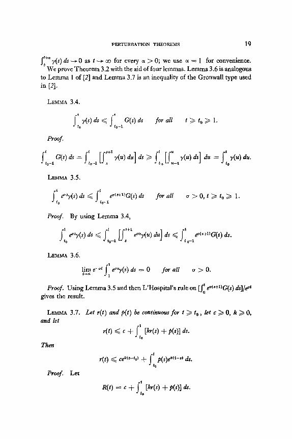
Jy y(s) a!s + 0 as t -+ co for every 01 > 0; we use OL = 1 for convenience. We prove Theorem 3.2 with the aid of four lemmas. Lemma 3.6 is analogous
to Lemma 1 of [2] and Lemma 3.7 is an inequality of the Gronwall type used in [2].
LEMMA 3.4.
Proof.
I” to-1
G(s) ds = It [j-‘+l y(u) du] ds 2 ,‘,, [j” y(u) ds] du = s;Oy(u) du. to-1 s U-l
LEMMA 3.5.
s t *, e”“r(4 ds < s t ~+~+l)G(s) ds for all cr > 0, t > t, >, 1. to-1
Proof. By using Lemma 3.4,
LEMMA 3.6.
I
t & e-*t Pi ds = 0 for all a > 0.
1
Proof. Using Lemma 3.5 and then L’Hospital’s rule on [Ji @+l)G(s) &I/P* gives the result.
LEMMA 3.7. Let r(t) and p(t) be continuous for t > t, , let c > 0, k > 0, and let
Then
40 < c + 11, [W + ~(41 ds.
Proof. Let
r(t) < cek(t-to) + s
~pp-.’ ds.
Jw = c + J:, [W + ml &

20 STRAUSS AND YORKE
Then R’ - kR <p. The result follows by integrating both sides from t, to t and solving for R(t).
Proof of Theorem 3.2 (using Brauer’s techniques). Let K 3 1 and u > 0 such that / eAt ) < Ke- ot for all t > 0. Let 0 < E < min(uK-r, r). From the hypothesis on $, choose T, and 6, so that 6, < E and T, > 1. Choose TO > T, so large that t 3 TO implies
K t e-k-Kd(t-S)y(s) & < ;.
1
This is possible by Lemma 3.6. Finally, let 6 = S,[2K]-1 and consider any t, > TO and x0 satisfying / X, 1 < 6. Then for as long as ( F(t, t, , %,,)I < 6, we have
t F(t) 7 eA+%hO + i tcl
eA+%#o, F(s)) ds + St eAt*-*)g(s, F(s)) ds, to
from which
1 F(t)1 < KSe-O(t-to) + I
IO [cKe-O(t-s) 1 F(s)1 + Ke-“(t-s)y(s)] ds
and
] F(t)] et < K&+0 + ,I, [EK [ F(s)] pa + Keoq(s)] ds.
Lemma 3.7 applied to r(t) = ) F(t)] t+ yields
/F(t)\ et < KGBtoeKc@-%) + KpBy(s)efK+s) ds, to
so that
1 F(t)1 < KSe-(~-~c)(t-to) + K e-(e-Krw-a)y(s) &, to
(34
hence
I F(t)1 < K6 + K J‘: e-(o-Kr)(t-s)y(s) ds < KS + 4 = 6, .
Thus, the inequality 1 F(t, t, , %,,)I < 6, holds on [to, co) which implies that (3.1) holds on [t,, , co), hence Ir;‘(t, t,, x,)1 + 0 as t --+ co. Since 6, < E, we have /F(t, to, x0)/ < E on [to, CO), which gives the asymptotic stability of x = 0 when g(t, 0) = 0, completing the proof.
Our final example shows that in a weak sense, condition (HI) is necessary in order that solutions tend to zero.

PERTURBATION THEOREMS 21
Example 3.8. Consider the first order equation
x’ = -ax + y(t), (3.2)
where a > 0, y(t) > 0 (this condition is removed in Theorem 4.7), and y does not satisfy (1 .l). Then there exists c1 > 0 and a sequence t, -+ a~ as n-+ cc such that jr y(t) dt > 01 for every 12. Then for every choice of x0 3 0 and t, >, 0,
F(t, t, , x0) = e-a(t-to)x, + ecat I
t t easy(s) ds > ecat
s easy(s) ds.
to to
Hence for all large n,
F(tlz + 1, t, , x0) > e-%+l) s
t,+1
easy(s) ds > e-%-t. t0
Thus F(t, t,, x0) + 0 as t --f CO, and the conclusion of Theorem 3.2 does not hold for (3.2).
4. PERTURBED NONLINEAR SYSTEMS
We start with a slightly more general theorem than that mentioned in the introduction.
THEOREM 4.1. Let x = 0 be U.A.S. andfG c,, on D, for (N). Let g(t, x) satisfy
(H,): There exists Y > 0 such thatfor every b, 0 < b < Y, there exist Q > 0 and a function Yb(t) continuous on [TV, 00) such that 1 g(t, x)1 < ra(t) for all b<IxI<randt>T,,whue
G@(t) = 1: yb(s) ds -+ 0 as t-+ co.
Then there exist T,, > 0 and 6, > 0 such that if t, >, T, and 1 x,, 1 < 6,) then the solution F(t, t, , x0) of (P) satisjes IF(t, t,, x,)1 -+O as t -+ co. In particular, ifg(t, 0) = 0, then x = 0 is U.A.S. for (P).
Proof. By Theorem 2.7, there exists a Lyapunov function V for (N) on D, satisfying
P(l x I) d WY 4 < EL(I x I>, (4.1)
%&, 4 G -(I x I), (4 *2)
I VW 41 < K, (4.3)
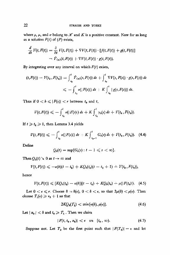
22 STRAUSS AN’D YORKR
where p, p, and o belong to X and K is a positive constant. Now for as long as a solution F(t) of (P) exists,
g w WN = 4 VP w + VV4F(t)) * [f(f, F(t)) + g(t,F(t))]
= G&, F(t)) + v w, F(t)) * g(4 F(f)).
By integrating over any interval on which F(t) exists,
Thus if 0 < b < 1 F(s)/ < I between t,, and t,
WW)) < - jt 41 WI) ds + K j” ~4s) ds + V(to >F(to)). to to
If t 2 t, 2 1, then Lemma 3.4 yields
W W)) < - j:, 41 WI) ds + K j: --1 G(s) ds + Wo , F(to)). (4.4) 0
Define Q&) = sup{G,(s) : t - 1 < s < co>.
Then Qr,(t) L 0 as t + co and
W, W) < --a@)(t - to) + KQdto)(t - to + 1) + Wo , F(to)),
hence
WWN G [KQ&o) - 4W - 4,) + ~Q&J + P(I%,N. (4.5)
Let 0 < E < r. Choose S = S(E), 0 < S < E, so that 2p(S) < p(c). Then choose TV 3 7s + 1 so that
2KQOJ < m44% p(4). (4.6)
Let 1 x0 1 < S and t, 2 Tr . Then we claim
I W, to, x0)1 < Q on Ito , a>. (4.7)
Suppose not. Let T, be the first point such that 1 F(T,)I = l and let

PERTURBATION THEOREMS 23
T2 < T, be the last point such that 1 F(T,)I = 6. Then 6 < ] F(t)] < e < Y on [T, , T3], hence by (4.5),
p(c) < V, , WA) < [KQdT,) - +W’s - TJ + KQtO’d + 4 Wd) G KQtdTd + ~(8) < MC> + id4 = f-J(~),
a contradiction, proving (4.7). This p roves the uniform stability of x = 0 for the case g(t, 0) = 0. For the rest of the proof choose 8, = S(Y) and T,, = T,(Y). Fix to >, T, and / x0 1 < 6, . Then (4.7) implies that I F(t, to, 41 -c 7 on [to , 00).
Let 0 < 77 < Y. Choose 8(~) and T,(q) as before so that (4.6) holds. Choose
T = [4Vdd + 2KQd) + W)l[491-’ > T&I)
and it is clear that T depends only on 7, not on to or x,, . We now claim
IF(tl,to,xo)l<S forsometrin [t,+T,,t,+T]. (4.8)
Suppose not. Then 1 F(t, to, xa)j > 6 on [to + TI , t, + T]. Let y. =F(to + Tl , to , x0). Then
0 < ~(4 G ~(1 Wo + T, 4, + TI 3 Y,,N < Wo + T Wo + TN G [KQ&o + Td - GW’ - TJ + KQdto + Td + ~(1 yo I) < -S+>(T - Tl) + KQ,(l) + P(Y) = 0,
a contradiction, proving (4.8). Thus by (4.7)
I F(t, 4 , F(tl , toy xo))l -=c rl on 15, co>
because t, > to + TI > TI and I F(t, , to , x,)1 < 6. Hence, a fortiori, I F(t, to, x0)1 < 7 for t >, to + T. Since 7 is arbitrary IF(t, to, x0)] + 0 as t --+ co. Since T depends only on 17 and 6 depends only on E, x = 0 is U.A.S. if g(t, 0) = 0, and the proof is complete.
Clearly, any function satisfying (Hr) satisfies (Ha). The converse is not true as the following example shows.
Example 4.2. Define g(t, x) = t[Px + 11-l. Then g does not satisfy (HI) because g(t, 0) = t, but g does satisfy (I&) with
and Tb = b-4 + 1, y&t) = t[t% - 11-1,
Gb(t) = [2b] log{[(t + 1)2b - l][t2b - 11-l).

24 STRAUSS AND YOFXE
The next example shows that the hypothesis “ x = 0 is U.A.S.” cannot be weakened to the condition “x = 0 is uniformly stable and E.A.S.”
Example 4.3. Consider the first order equations
x’ = -(t + 1)-1x, (4.9)
x’ = -(t + 1)-1x + 2(t + 1)-1x = (t + I)-%. (4.10)
Then x = 0 is uniformly stable and E.A.S. for (4.9), the perturbation term 2(t + I)-lx in (4.10) satisfies (HI), but all nontrivial solutions of (4.10) are unbounded.
The condition f E c,, on D, need not hold, however. The existence of a Lyapunov function satisfying (4.1), (4.2), and (4.3) is sufficient for the conclusion of Theorem 4.1, and such a function may exist even though
fGo9 as can be seen below.
Example 4.4. Consider the first-order equation
x’ = -(t + 1)x, (4.11)
whose right-hand side is not in c,, , yet the function V(t, x) = x2 satisfies (4.1), (4.2), and (4.3). Thus (4.11) can be perturbed by a function satisfying (H,), although Theorem 4.1 as stated does not apply to (4.11).
We now consider the possibility of integrating the perturbation term before obtaining bounds on its norm. Specifically, consider the condition (Ha): Let h(t) be continuous on [0, co) and let H(t) be a continuous, nonincreasing function with H(t)+ 0 as t + co such that
1 j:oh(s)ds 1 < H(t,) for every 0 < t, < t < t, + 1.
Then any function h(t) for which Jy 1 h(s)/ ds -+ 0 as t + co satisfies (Hs), so that perturbation terms independent of x which satisfy (HJ also satisfy (Ha). Example 4.5 shows the generality of (Hs).
Example 4.5. Let h(t) = (t sin t3, t cos t3). Then h(t) does not satisfy (HI) because 1 h(t)1 -+ co and hence ly 1 h(s)1 A+ co, as t-+ co. But h(t) satisfies (Ha), because, for example,
IS t to
scoss3d~I = IjI[~cos~‘-~sinSB]d~+j~~$sin~3d~I
< 1[$-sins3]~o 1 + jlo&ds

PERTURBATION THEOREMS 25
THEOREM 4.6. Let x = 0 be U.A.S. and f E CO on D, for (N). Let g sattify (El,) und h satisfy (H3). Then there exist T,, > 0 and 6, > 0 such that if t, > Z’, and 1 x0 1 < 6, , the sohtion F(t, t, , x0) of
x’ =f(t, x) + g(t, x) + h(t) (PI)
sutis$es 1 F(t, t, , .x0)/ -+ 0 us t + 00.
Proof. In deriving the analog of (4.4) for the system (PI), we are led to
+ j” VV(s, W)) * 4s) ds + V(to ,F(t,)). to
(4.12)
Thus, we must estimate 1 St”, V V(s, F(s)) * h(s) ds I. Let J(t) = JiO h(s) ds. Then
s t VV(s,F(s)) - h(s) ds to
= s:, vv(s, F(s)) *F’(s) ds + s:,; V(s, F(s)) ds - ,:, ; v(s, WI ds
- s 1, v w WN * [f(s, F(s)) + As, W)l ds
+ f, VW F(s) - J(s)) . [f (s, F(s)) + g(s, @))I ds
- s :, VW w - J(S)) * [f(s* F(s)) + & W)l ds
+ s:,; Vh F(s) - J(s)) ds - f, ; V’(s, F(s) - J(s)) ds
= w, F(t)) - w F(t) - J(t))>
+ slo I$ Wt W - J(s)> - ; % W( ds
+ jlo {VW F(s) - l(s)) - V V, fW)l * lf(s, W) + g(s, W)) ds.
We shall now use two facts which were not needed before; namely, ,f is bounded on D, and V satisfies
I VP, 4 - VP, r)l < A I x - Y I,
lVW4--V(t,y)l <Alx--yl,

26 STRAUSS AND YORKFi
and
on D, for some constant A > 0. This latter fact holds because the first and second partials of V are bounded on D, (by Theorem 2.7), while the former holds because f E r?,, andf(t, 0) = 0.
Let jf(t, x)1 <B on D,. Temporarily, let 0 < t - t,, < 1. Then
I J(t)1 < Wo). Thus
d PA + AWVo) + AHGo) j: --1 GA4 ds
= [2A + AB]N(GJ + Afqt,) +“~ws)Qa(s)(t - to + 1)
< P4 + AB + 2AQ,(toWPo)-
Thus for arbitrary t > to ,
1 j;, VW, F(s)) . 4s) ds /
< 1 j;:' VV(s, F(s)) - 44 ds ( + -.- + / j; VW, F(s)) - 4s) ds 0 +nl j
< 42 + B + 2Q&oVWo) + e-0 + 42 + B + 2Qdto + 4lWo + 4
d 42 + B + 2Q&oWWo) + *.- + 42 + B + 2Q&o)lWo)
< 42 + B + 2Q&oW(~o)[~ - to + 11.
The proof now proceeds as the proof of Theorem 4.1. If g(t, X) = 0 in (Pi), then the condition (Hs) on h(t) becomes necessary
for the solutions to tend to zero.
THEOREM 4.7. Let x = 0 be U.A S. and f e co on D, for (N). Then the conclusz~otz of Theorem 4.6 hola5 for the system
x’ =f(t, x) + h(t) (Pa)
if and only if h(t) satzijies (HJ.
Remark. In (Pz), h(t) is a vector; compare this result with Example 3.8.

PERTURBATION THEOREMS 21
Proof. Let h satisfy (Ha). Then the conclusion of Theorem 4.6 holds for (P2) by Theorem 4.6.
Conversely, suppose that h does not satisfy (Ha). Then there exist 01 > 0 and sequences (tn} and {E,}, with 0 < E, < 1 for every n and t, + co as II -+ co, such that
is %I+(”
h(t) dt > 01 (4.13) L
for every n. Assume (we shall contradict this assumption) that there exist some t, > 0 and some x,, for which the solution F(t, t, , x0) of (PJ satisfies j F(t, t, , x,)1 + 0 as t -+ co. Choose T so large that t > T implies
where L is the Lipschitz constant for f and we may assume without loss of generality that L > 1. Then for n so large that t,, > T, we have
Lf4 h(t) dt
t” I
Z=Z 1 /;;f(t,F(r. t, , 4) dt + j::I’.F’(t, t, , x,,) dt j
G i tn+p”L I F(t, to 7 xo)l dt + I Wa + 6% , to , xc,)1 + I F(tn , to , x0)1 t”
a contradiction to (4.13). Thus no solution of (P2) tends to zero as t -+ 03 hence the conclusion of Theorem 4.6 certainly does not hold, completing the proof.
5. PERTURBED NONLINEAR SYSTEMS: A SECOND PROOF
THIDREM 5.1. Let x = 0 be U.A S. and f cz co on D, for (IV). Let g satzify (HI) and h satisfy (HJ. Then there exist To 3 0 and 6, > 0 such that if to > To and I x0 1 < So, the solution F(t, to, x0) of (PI) satisjies / F(t, to, x0)] -+ 0 us t--f co. In particdur, if g(t, 0) = 0 and h(t) = 0, then x = 0 b U.A S. for (PI)
This result is not as general as Theorem 4.6 because here we need f E co even for the case h(t) z 0 (see Example 4 4), and also because we assume g satisfies (HI) rather than (Ha) However, the proof does not require Lyapunov functions, which is rather curious. Furthermore, almost no extra effort is
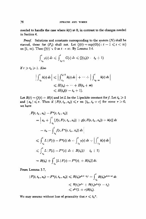
28 STRAUSS AND YORKE
needed to handle the case where h(t) + 0, in contrast to the changes needed in Section 4.
Proof. Solutions and constants corresponding to the system (N) shall be starred, those for (PI) shall not. Let Q(t) = sup(G(s) : t - 1 < s < CD} on [I, co). Then Q(t) L 0 as t + co. By Lemma 3.4.
j’,, Y(S) ds < 1” G(s) ds < Q(to)(t - to + 1) to-1
ift>t,>l.Also
< Wo) + *.. + fqtll + m) < fqto)(t - tll + 1).
Let B(t) = Q(t) + H(t) and let L be the Lipschiti constant forf. Let to > 1 and lx,,] <r. Then if IF(t,t,,x,)l<r on [tO,to+T] for some T>O, we have
I F(t, to , x0) - F*(t, to P x0)1 = x0 + I s 1, MS, m, to , ~0)) + As, F(s, to 3 ~0)) + WI ds
- xo - s t f(s, F*(s, to , xo)) ds 1 to
< j-” L I F(s) - F*(s)1 ds + s:, Y(S) ds + 1 J:oh(4 ds / to < s t L I F(s) - F*(s)1 ds + B(t,)(t - to + 1)
to
= B(to) + St CL I F(s) - F*(s)1 + %)I ds. to
From Lemma 3.7,
I W, to , x0) - F*(t, to , x,)1 Q B(to)&‘t-to’ + St 13(to)e=‘t-S’ ds to
We may assume without loss of generality that Y < 6,*.

PERTURBATION THEOREMS 29
Let 0 < E <Y. Choose S = a(~) = S*(42) so that 0 < 8 < E. Choose T = r(e) = T*(6/2). Choose Tl = T,(r) > I so large that
B(T,) < a[@(1 + 7)21-l.
Let t, > Tl and ) x0 1 < 6. Then for as long as 1 F(t, t, , x,)1 < E in the interval [to , t, + 5-1,
IF(t) to > x,,)l < I F(t, to, xo) - F*(t, to, xo)l + I F*(t, to, xo)l
< f+T(l + T)B(t,) + 42
< +(l + T)B( Tr) + 42
< 612 + 42 < E/2 + 42 = E.
Since E < Y, F(t, t, , x,,) can be continued to [to , to + T] on which 1 F(t, to , x0)1 < E. Let x1 = F(to + T, to, x,,). Then
I X1 1 d / X1 - F*(to + 7, t, , X,)1 + I F*(t, + ‘-, to , X,)1
< W + I F*(to + 7’*(W), to, xo)l
< 812 f 612 = 6.
Now let m be a positive integer and assume that 1 F(t, to , x,)1 < E on [to, to + mT] and [ F(to + mT, to, s)i < 6. Let x, = F(to $ mT, to , x0). Then for as long as 1 F(t, t, + mT, x,)1 < E on the interval [to + mT, to + (m + I)T],
we have
I F(t, to + mT, x,>l < I F(t, to f 1127, %) - F*(t, to -I- mT9 4
+ I F*(t, to + mT, x,)1
< p( 1 + T)B(to + mT) + 4 < 612 + 42 < E.
Since E < Y, F(t, to, x0) can be continued to the entire interval [to + mT,
to + (m + l)~] on which ) F(t, to, x0)1 < E. Let x,+r = F(to + (m + l)T, to, x0). Then
1 %+, 1 < IF(to + (m + 1)~~ to + mT, xm> -F*(to + (m + 1)~~ to + mT, x,)l
+ I F*(t, + (m + lb, to + 1127, x,)1
< 612 f 612 = 6.
Thus, by induction, ] F(t, to, x0)1 < E on every interval [to + mT,
to + (m + l)~], and hence on [to, co). Hence if g(t, 0) = 0 and h(t) = 0, then we have shown that x = 0 is uniformly stable. For the rest of the proof, choose 6, = S(Y) and To = T,(Y). Fix to > To and I x0 / < 6, . Then I W to9 x0)1 < r on [to , ~0).
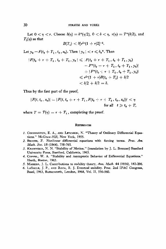
30 STRAUSS AND YORKE
Let 0 < 7 < Y. Choose 6(r)) = S*(77/2), 0 < 6 < 1, ~(7) = T*(8/2), and T,(q) so that
I?( Tl) < S[P( 1 + 421-l.
Let y0 = F(tO + T, , t, , x,,). Then ) y,, 1 < T < a,*. Then
I~(~o+~+~l,~o+~l,YoI~I~(~,+~+~l,~o+~l,Yo)
- F*(to + T + Tl, to + Tl, YJI
+ lF*(t,+~+Tl,t,+T,,~,)l
< @‘(I + T)& + Td + 6/2
< 612 + 612 = 6.
Thus by the first part of the proof,
where T = T(T) = 7 + Tl , completing the proof.
RRFIMNCFS
1. CODDINGTON, E. A., AND LWINSON, N. “Theory of Ordinary Differential Equa- tions.” McGraw-Hill, New York, 1955.
2. BRAUER, F. Nonlinear differential equations with forcing terms. Proc. Am. Math. Sot. 15 (1964), 758-765.
3. KRASOVSKII, N. N. “Stability of Motion.” [translation by J. L. Brenner] Stanford University Press, Stanford, California, 1963.
4. COPPEL, W. A. “Stability and Asymptotic Behavior of Differential Equations.” Heath, Boston, 1965.
5. MASSERA, J. L. Contributions to stability theory, Ann. Math. 64 (1956), 182-206. 6. LASALLE, J. P., AND RATH, R. J. Eventual stability. Proc. 2nd IFAC Congress,
Basel, 1963, Butterworth, London, 1964, Vol. II, 556-560.