Journal of Computat ional and Applied Mathematics 10 (1984) 113-132 113 North-Holland

Algorithm 27

A method for the numerical inversion transforms

of Laplace

G. HONI G * Departamento de Inform4tiea, Pontifica Universidade Catrlica, Rio de Janeiro, Brasil

U. HIRDES lnstitut fi~r FestkOrperforsehung, Kernforschungsanlage Ji~lich, Germany, Fed. Rep.

Received 19 February 1980 Revised 4 July 1983

Abstract: In this paper a numerical inversion method for Laplace transforms, based on a Fourier series expansion developed by Durbin [5], is presented. The disadvantage of the inversion methods of that type, the encountered dependence of discretization and truncation error on the free parameters, is removed by the simultaneous application of a procedure for the reduction of the discretization error, a method for accelerating the convergence of the Fourier series and a procedure that computes approximately the 'bes t ' choice of the free parameters. Suitable for a given problem, the inversion method allows the adequate application of these procedures. Therefore, in a big range of applications a high accuracy can be achieved with only a few function evaluations of the Laplace transform. The inversion method is implemented as a F O R T R A N subroutine.

Keywords: Numerical integration, Laplace transforms, numerical Laplace inversion.

1. Introduction

The significance of numerical Laplace inversion is obvious from the big range of applications. Well known in engineering, Laplace transformation methods are also used in order to solve differential and integral equations and to assist when other numerical methods are applied (see [7,10]).

A number of numerical inversion methods has been developed during the last few years. In what follows we confine ourselves to the methods using Fourier series approximations. Many tests (see [1,2,4,5,8] have demonstrated the simplicity and the accuracy of these methods.

Fourier series were first used by Dubner and Abate [4] in 1968 for the numerical inversion of Laplace transforms. Durbin [5] improved the method in 1973.

Other authors, Simon et al. [8] in 1972, Veillon [9] in 1974 and Crump [2] in 1976, used different acceleration methods in order to speed up the convergence of the Fourier series derived in [4,5]. Some of these methods at times achieve a considerable reduction of the truncation error. However, they fail in other cases and their efficiency heavily depends on the choice of the parameters of the methods of Durbin or Dubner and Abate, and the choice of these parameters was somewhat arbitrary.

The biggest disadvantage of the above mentioned methods is the dependence of the discretization and

* Present address: Deuzer Maschinenfabrik GMBH, Postfach 3165, D5902 Netphen 3, Germany, Fed. Rep.

0377-0427/84/$3.00 © 1984, Elsevier Science Publishers B.V. (North-Holland)

114 G. Honi~ U. Hirdes / Laplace transform

truncation errors on the free parameters: by a suitable choice of these parameters the discretization error becomes arbitrarily small, but at the same time the truncation error grows to infinity and vice versa. A first step in surmounting this problem was taken in [1], (see Section 3), where the so-called 'Korrektur ' -method was presented. It allows a remarkable reduction of the discretization error without increasing the truncation error.

Nevertheless the accuracy of the 'Korrektur ' -method also depends on a 'good' choice of the free parameters. The procedure introduced in Section 5 gets closer to the solution of the problem. It allows the approximate computation of optimal parameters for all above mentioned methods (for the definition of 'opt imal ' see Section 5).

Section 4 describes a new method for the acceleration of convergence of the Fourier series. It is applicable if the infinite series for the approximation of the inversion integral does not alternate (see Section 4). In this case all other tested acceleration methods fail.

Finally, in Sections 2 and 4, those of the above mentioned inversion and acceleration methods that were found to be best by numerical tests as well as by the derived error estimates are summarized.

A new algorithm for the numerical Laplace inversion, taking into consideration the new, above mentioned, procedures and implemented as a F O R T R A N subroutine 1 is described in Section 6.

This subroutine can be used as a 'b lack box': the only input parameters are the t-values for which f ( t) = L-I[F(s)] shall be computed and of course the Laplace transform F(s). On the other h a n d - - f o r a concrete p rob lem- - the user can make an optimal choice of all free parameters in order to have the most efficient combination of the algorithms contained in the subroutine.

The efficiency of the inversion method is shown by the examples in Section 7.

2. The method of Durbin

The Laplace transform of a real function f : R ~ R with f ( t ) = 0 for t < 0 and its inversion formula are defined as

F(s) = L[f(t)] =f0 °~ e - ' t f ( t ) d t , (1)

1 f~+i~ eS,F(s)ds, f ( t)= L-l[ F(s)] = T~i o-i~ (2)

with s = v + iw; v, w ~ R. v c R is arbitrary, but greater than the real parts of all the singularities of F(s). The integrals in (1) and

(2) exist for Re(s) > a ~ R if

(a) f is locally integrable, (b) there exist a t o >/0 and k, a ~ R, such that If( t)[ ~< k e ~t for all t >/t 0, (3) (c) for all t ~ (0, ~ ) there is a neighbourhood in which f is of bounded variation.

In the following we always assume that f fulfils the conditions (3) and in addition that there are no singularities of F(s) to the right of the origin. Therefore (1) and (2) are defined for all y > 0. The possibility to choose v > 0 arbitrarily, is the basis of the methods of Dubner -Aba te and Durbin. The latter is now described.

Using the inversion formula (see [5])

f ( t ) =--~-e°'f~[Re{F(S)~o } cos(wt) - I m ( F ( s ) } sin(wt)]dw, (4)

1 See Appendix A, subroutine LAPIN (LAPlace INversion).

G. Honig, U. Hirdes / Laplace transform 115

which is equivalent to (2), and a Fourier series expansion of h ( t ) = e "' f(t) in the interval [0, 2T], Durbin derived the approximation formula

f ( t ) = - ~ - - ½ R e { F ( v ) } + Y'~ Re F v+ , - -~- k = 0

x c o s - ~ - t - ~ Im f v+i sin ~--t -r l (v , t , r ) , (5) k = 0

for 0 < t < 2T. Fl(v, t, T) is the discretization error, given by

FI(v, t, T) = £ e-2"krf(2kT+ ,). (6) k = l

Since there are no singularities of F(s) in the right halfplane we have (see [3, Bd. 1]) a c > 0, rn >~ 0 and a t o >/0, such that

[ / ( t ) ] ~< ct m for allot > t 0. (7)

From (6) and (7) the following estimates for the discretization error can be deduced (see [5]):

(a) m = 0,

C [ r a ( v , t, T)[ ~ < - - , (8)

e 2re - - 1

(b) m > 0,

iFl(v,t,T)l<K(2T)me_2,,r( a, am+,) + " - + - - - - , (9) (2 v) m+'

where K, a I . . . . . a, ,+l ~ R. These estimates show that the discretization error can be made arbitrarily small by choosing v

sufficiently large. As the infinite series in (5) can only be summed up to a finite number N of terms, there also occurs a

truncation error given by

ImI ( + k=N+l ~ - - t - - i sin ~-- t .(10)

Hence the approximate value for f(t) is

= e " ' [ - 1 R e { F ( v ) } + ~ { R e { F ( o + i ~ - ~ ) } ~-~t fN(t) ~- k=0 COS

- Im{F(v+i~)}sin ~-~t}]. (11)

3. The reduction of the discretization error by the 'Korrektur'-method

It is obvious from (8) and (9) that the discretization error can be made arbitrarily small if the product vT is sufficiently large.

Unfortunately, the truncation error (10) may diverge for large values of vT.

116 G. Honig, U. Hirdes / Laplace transform

The 'Kor rek tu r ' -me thod allowes a reduction orf the discretization error without enlarging the truncation error. With (11), equation (5) can be written in the form

f ( t ) = f ~ ( t ) - F l ( v , t, T ) . (12)

The 'Kor rek tu r ' -me thod uses the approximat ion formula

f ( t ) = f ~ o ( t ) - e 2"vf~(ZT+ t ) - r Z ( v , t, T ) . (13)

As stated in the theorem below, the discretization error F2(v, t, T ) is much smaller than FI(v, t, T). Taking into considerat ion the truncation error (10), we find that the approximate value for f ( t ) , using

the 'Kor rek tu r ' -me thod (13), is given by

fuK ( t ) = fN( t ) -- e- Z~TfNo(ZT + t ). (14)

It should be ment ioned that the truncation error of the 'Kor rek tur ' - t e rm e - 2 " T f ~ ( 2 T + t), is much smaller than FA(N, v, t, T) if N = N 0. We can therefore choose N o < N (see Section 6), which means that only a few additional function evaluations of F(s) are necessary to achieve a considerable reduction of the discretization error. This error reduction is pointed out in the following theorem.

Theorem 3.1. Suppose f is a real function with f ( t ) = 0 for t < 0 that possesses the properties (3) and F(s ) = L[ f ( t ) ] its Laplace transform that has no singularities to the right of the origin, and suppose the "Korrektur '-formula (13) is used for the numerical inversion of F( s ), then

2e (a) IF2(v , t, T ) l < i f m = O , (15)

eZ~'r(e 2vT- 1)

(b) , F 2 ( v , t , T ) l ~ 3 " e - 2 ~ T { K ( 2 T ) " e - 2 V r ( a' a"+, ) ) ~ - ~ + . . - + (16) (2vT) " + '

if m > 0 and ( m ! ) / 2 " - 1 -%< 2vT.

For the definition of c, m, K, a 1 . . . . . a,,+~ see equations (7), (8) and (9). For the proof see [1] or [6].

Remarks. A compar ison with the method of Durbin (see (8) and (9)) shows a reduction of the error bound by the factor 2e-2v T for m = 0 and 3" e -2vr for m > 0. The condit ion m ! / 2 " - 1 ~ 2vT might be difficult to fulfill for large m, and hence the application of the 'Kor rek tu r ' -me thod is not recommended in such

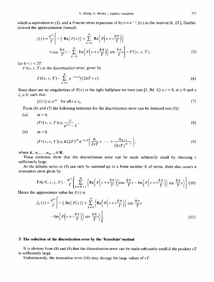
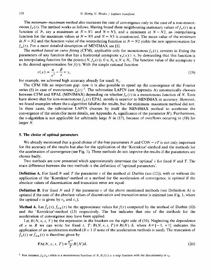
cases. As ment ioned before, an adequate reduction of the total error can be obtained by the ' Korrektur ' -method

only if (for fixed N and T) the parameter v is suitable. This is illustrated in Fig. 1. It shows the error curves

0 0015 o

00010 o

o 0 0005

00000 0

Fig. l.

IF21+IFAI~t~

1

~ IF I I * IFAI

I F 2 1 ~ Fll ~ , _

vl T Vo T 3 4 ~T

G. Honig, U. Hirdes / Laplace transform 117

of the method of Durbin (F1 and FA) and of the 'Korrektur ' -method (F2 and FA). A successful application of the 'Korrektur ' -method requires a v < %. For v > v 0 the truncation error dominates and the reduced discretization error F2 does not lead to a noticeable reduction of the total error.

The opposite holds if the methods for the acceleration of convergence, that we describe in the following part, are applied. Acceleration of convergence is only sensible if v > v 0 or, which is the same, if the truncation error dominates.

However, a simultaneous application of an acceleration method and the 'Korrektur ' -method (as realized in the subroutine LAPIN) is recommended, if the parameters are optimally chosen by the procedures introduced in Section 5.

4. Acceleration of convergence

In this section three acceleration methods used in the subroutine LAPIN (see Appendix A) are briefly described: the e-algorithm, the min imum-max imum method and a method based on curve fitting. The latter is new, whereas the e-algorithm was already used in [2,9], the min imum-max imum method in [1] in order to speed up the convergence of the series approximating the Laplace inversion integral. We have also tested other acceleration methods such as the Euler transformation, or Aitken's extrapolation p rocedure (see [8]). But these turned out to be less efficient than the above mentioned methods.

We can consider f h ( t ) (see (11)) for fixed t as a discrete function of N and define:

Definition. fN(t) as a function of N is monotonous if

IfN(t) - - f~ (t)] >~ IfM(t) - - f ~ ( t ) [

for all N, M with N ~< M.

For a non-monotonous fN(t) the e-algorithm (EPAL) and the min imum-max imum method (MINI- MAX) in general significantly increase the rate of convergence. However, they fa i l - -as do the Euler transformation and Aitken's extrapolation procedure- - for a monotonous fN(t). The method based on curve fitting (CFM) leads in this case to a considerable improvement in the results. With

c k ,= -~ - Re F v + i cos T t - I m

we can replace (11) by

N

fN(t)=½Co + E Ck" k = l

The e-algorithm applied to (17) is defined as follows: Let N = 2 q + 1, q~N,

S m := ~ Ck k = l

and

v+l--~-- s i n - f - t , k = 0 , 1 , 2 . . . . .

(17)

~°~+1) - e(pm') e~om' '= O, ( "~ ' - (18) (,,1) .__ ( r e + l ) + 1 / ( e p Ep + 1 "-- Ep _ 1 ~ E1 "-- Sm '

then the sequence e~ 1), E~ 1), or1) oo) = e~ ), converges to foo(t)-Co/2. For a non-monotone fN(t) in ~5 , ' ' ' , ~ 2 q + l

general it converges faster than the sequence of the partial sums s,,, m = 1, 2 . . . . of the untransformed series.

118 G. Honig, U. Hirdes / Laplace transform

The minimum-maximum method also increases the rate of convergence only in the case of a non-monot- onous fN (t). The method works as follows. Having found three neighbouring stationary values of fN (t) as a function of N, say a maximum at N = N1 and N = N3, and a minimum at N = N2, an interpolating function for the maximum values at N = N1 and N = N3 is constructed. The mean value of the minimum ~it N = N2 and the function value of the interpolating function at N = N2 yields the new approximation for f~( t ) . For a more detailed description of MINIMAX see [1].

The method based on curve fitting (CFM), applicable only for monotonous fN (t), consists in fitting the parameters of any function that has a horizontal asymptote "/A(X) -- ~', by demanding that this function is an interpolating function for the points (N, fN(t)), 0 <~ N O <~ N <~ N 1. The function value of the asymptote ~, is the desired approximation for f ( t ) . With the simple rational function

r ( x ) : = 7 + - - + Y, (19)

for example, we achieved high accuracy already for small N t. The CFM fills an important gap: now it is also possible to speed up the convergence of the Fourier

series (5) in case of monotonous f , ( t ) 2. The subroutine LAPIN (see Appendix A) automatically chooses between CFM and EPAL (MINIMAX) depending on whether/N (t) is a monotonous function of N. Tests have shown that for non-monotonous fN (t) EPAL mostly is superior to MINIMAX in accuracy. However, we found examples where the e-algorithm falsifies the results, but the minimum-maximum method did not. In these cases, the subroutine LAPIN chooses by itself the MINIMAX method to accelerate the convergence of the series (for more details, see Appendix A, significance of the parameter H). Furthermore, the e-algorithm is not applicable for arbitrarily large N in (17), because of overflows occuring in (18) for larger N.

5. The choice of optimal parameters

We already mentioned that a good choice of the free parameters N and CON = vT is not only important for the accuracy of the results but also for the application of the 'Korrektur '-method and the methods for the acceleration of convergence (see Fig. 1). These methods do not improve the results if the parameters are chosen badly.

Two methods are now presented which approximately determine the 'optimal' v for fixed N and 7". The main difference between the two methods is the definition of 'optimal parameters'.

Definition A. For fixed N and T the parameter v of the method of Durbin (see (12)), with or without the application of the 'Korrektur '-method or a method for the acceleration of convergence, is optimal if the absolute values of discretization and truncation error are equal.

Definition B. For fixed N and T the parameter v of the above mentioned methods (see Definition A) is optimal if the sum of the absolute values of discretization and truncation error is minimal (see Fig. 1, where the optimal v is given by v 0 and vl).

Method A. Let fN(t) , fNK(t) be the approximate values for f ( t ) computed by the method of Durbin (12) and the 'Korrektur '-method (13) respectively. The bar indicates that one of the methods for the acceleration of convergence may have been applied.

Let R(N, v, t, T) be the expression in the brackets on the right side of (10). Neglecting the dependence of v in R we can write for fixed t, T: R(N, v, t, T ) - - R ( N ) . & where 3 E [ - 1 , +1] indicates the application of an acceleration method (6 = 1 if none of the acceleration methods is used). The truncation of fN( t ) or fNK(t ) is therefore given by

eV' (20) FA(N, v, t, T) =--~-R( N ) 8 .

2 For instance, fN(to) often is a monotonous function of N, if f(t) is a step function with the discontinuity in t 0.

G. Honig, U. Hirdes / Laplace transform

With (5), (6) and (20) we find

iN(t) my(t) - ~-~ R( N)3 + O(e-2"T).

Let vl, 02 be large and v I 4:v23, then

f~v( t) --]2u( t ) ~ R( N )3. (e °2'- eV't)/T

o r

• • • t • R ( N ) 3 - - T "~'*'t" eVz t _ eO,t

Similarly we get for the 'Korrektur'-method

R ( N ) 3 --- T f/~K(t) ~ f ~ K ~ t ~ cO2 t _ colt

The discretization error (6) of the method of Durbin can be written as (see Section 6)

Fl (o , t, T) = e -~°7(2T + t) + O(e-4vT).

From (13) we find for the discretization error of the 'Korrektur'-method

F 2 ( o , t , T ) = ~ e - 2 V r k ( f ( 2 k T + t ) - f ( 2 T ( 3 k - 2 ) + t ) } . k = 2

Hence

119

(21)

(22)

(23a)

(23b)

(24a)

F2(v, t, T) = e 4vT( f ( 4 T + t) - f ( 8 T + t)} + O(e-6Vr). (24b)

Using Definition A, the equations (23) and (24) easily lead to the following equations for the optimal parameter v = VoAvr:

1 In R ( N ) 3 I (method of Durbin) vAvr-- 2 T + t TfN(2T+t ) (25a)

I and

1 In R ( N ) 6 (' Korrektur'-method). (25b) V°ar'r = 4 T + t T{ fN(4T+ t ) - ) ~ ( 8 T + t)}

Because of Definition A an upper bound for the total absolute error I f ( t ) - - fu ( t ) l or I f ( t ) - - fuK( t ) l for v = vAvr is approximately given by

/)ApT • l

TERR -= 2 ~ I R ( N ) 3 I. (26)

Method B. We now use Definition B and assume that R(N, v, t, T) is no longer a constant function of v to get a more accurate approximation formula for Vop T.

The dependence of v is assumed to be as follows (R(N, v, t, T)= R(N, v)8 because t, T are fixed, v~ > 0 arbitrary):

R ( N , v ) 3 = - R ( N , va)3. Re F v + i c o s - ~ - - - t - I m F v + l - - T- sin--~-t

/[Re(F(vt+i-~-)}cos--~-tN¢r _ i m { F ( v l + i _ _ ~ ) ) s i n L "n ] 1 t ] - i (27)

3 We found that for example v~ ,= 20, v 2 ,= v I -2 is a good choice.

120 G. Honig, U. Hirdes / Laplace transform

The acceleration factor 8 can be computed very easily from (23a) without additional function evaluations:

8 = (28) f~ ( t ) --UZN(t )

Let AR(v~, v, N ) be the expression in brackets on the right side of (27) and R(N, vl)8 ,= R ( N ) & where R(N)8 is computed by Method A. then (27) is expressible in the form

R( N, v)8 = R( N)8 . AR(vl , v, N ) . (29)

Definition B implies (for the method of Durbin);

e. ] = 0. ( 3 0 ) [R(N, v )81~-+lFl (v , t, T)I , ..... ,%T

Approximating the derivative of R(N, v) by finite differences, we find the following iteration procedure to solve equation (30):

R(N, v) --- (31a) u ( i - 1) __ U~ i-1)

v (°) = oAvr, V~ °, = v I , (318)

v~ i) = v (i-t), i = 1 . . . . . s - 1. (31c)

v(i) 1 In ~v]R(N'v)(°18 + [ R ( N ' v (i 1))16.t = , i = 1, 2 . . . . . s. (31d)

2 T + t 2 T 2 l f u ( 2 T + t) I

In (31b) v~zr and v 1 are defined by Method A (see equation (25) and (22) respectively). Equation (31d) follows from (30) substituting (31a) for the derivative of R(N, v) and (24a) for F l ( v , t, T).

Hence the optimal parameter v = VoBvr for fixed N, T, t is given by

VoB r = v ( ' . ( 32 )

An analogous result holds for the 'Korrektur ' -method: Replacing F1 by F2 in (30), we only have to substitute (31d) by

v(~)= 1 In , i = 1, 2 . . . . . s. (31e) 4 T + t 4TZ[?N(4T+ t) --fN(8T+ t)l

It is sufficient to choose s = 1 or s = 2, as numerical tests have shown. Again it is possible to compute approximately an upper bound for the total error, if the parameter

v = v~v r is used for the computation of fN (t) a. We find

v~°"t 2°"°~rlfN(2T+ t)l. (33) TERR----e ~ IR(N, voBvr)l 8 + e -

Remarks. The simplifications made in order to derive equations (25) and (31) do in general not cause any difficulties. Besides a few exceptions, which are discussed later, the optimal parameters VoApT and VoBvr are a good approximation for the true optimal parameters.

If the e-algorithm is used in order to accelerate the convergence of the series (5), it is not possible to compute the acceleration factor 8 for large N with the desired accuracy (the e-algorithm breaks down after a certain N O < N depending on v, t and T; N O is not known in advance; see also the final remarks of Section

4 A similar equation holds forfNK(t).

G. Honig, U. Hirdes / Laplace transform 121

4). Therefore the minimum-maximum method allows a more accurate determination of the optimal parameters by Method A or B, and hence of the total error (26) or (33).

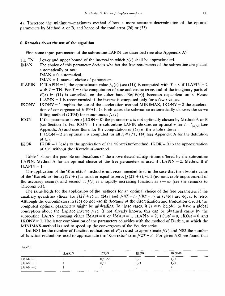
6. Remarks about the use of the algorithm

T1, TN IMAN

First some input parameters of the subroutine LAPIN are described (see also Appendix A):

Lower and upper bound of the interval in which f ( t ) shall be approximated. The choice of this parameter decides whether the free parameters of the subroutine are placed automatically or not: IMAN = 0 automatical, IMAN = 1 manual choice of parameters.

ILAPIN If ILAPIN = 1, the approximate value fN(t) (see (11)) is computed with T = t, if ILAPIN = 2 with T = TN. For T = t the computation of sine and cosine terms and of the imaginary parts of F(s) in (11) is cancelled, on the other hand Re{F(s) ) becomes dependent on t. Hence ILAPIN = 1 is recommended if the inverse is computed only for a few t-values.

IKONV 1KONV = 1 implies the use of the acceleration method MINIMAX, IKONV = 2 the accelera- tion of convergence with EPAL. In both cases the subroutine automatically chooses the curve fitting method (CFM) for monotonous fu(t ).

ICON If this parameter is zero (ICON = 0) the parameter v is not optimally chosen by Method A or B (see Section 5). For ICON = 1 the subroutine LAPIN chooses an optimal v for t = tls/2 J (see Appendix A) and uses this v for the computation of f ( t ) in the whole interval. If ICON = 2 an optimal v is computed for all t k ~ (T1, TN) (see Appendix A for the definition of t,).

IKOR IKOR = 1 leads to the application of the 'Korrektur'-method, IKOR = 0 to the approximation o f f ( t ) without the 'Korrektur'-method.

Table 1 shows the possible combinations of the above described algorithms offered by the subroutine LAPIN. Method A for an optimal choice of the free parameters is used if ILAPIN = 2, Method B if ILAPIN = 1.

The application of the 'Korrektur '-method is not recommended first, in the case that the absolute value of the 'Korrektur '-term f (2T + t) is small or equal to zero: ]f(2T + t)l<< 1 (no noticeable improvement of the accuracy occurs), and second, if f ( t ) is a rapidly increasing function as t ~ oo (see the remarks to Theorem 3.1).

The same holds for the application of the methods for an optimal choice of the free parameters if the auxiliary quantities (these are f ( 2 T + t) in (24a) and f ( 4 T + t ) f ( 8 T + t) in (24b)) are equal to zero. Although the denominators in (25) do not vanish (because of the discretization and truncation errors), the computed optimal parameters might be misleading. In these cases, it is very helpful to have a global conception about the Laplace inverse f(t) . If not already known, this can be obtained easily by the subroutine LAPIN choosing either IMAN = 0 or IMAN = 1, ILAPIN = 2, ICON = 0, IKOR = 0 and IKONV = 1. The latter combination of the parameters coincides with the method of Durbin, at which the MINIMAX-method is used to speed up the convergence of the Fourier series.

Let NS1 be the number of function evaluations of F(s) used to approximate f ( t ) and NS2 the number of function evaluations used to approximate the 'Korrektur '-term f (2T + t). For given NS1 we found that

Table 1

ILAPIN ICON IKOR IKONV

IMAN = 1 1 0 / 1 / 2 0 / 1 1 / 2 IMAN = 1 2 0 / l 0 / 1 1 / 2 IMAN = 0 l 1 0 2

122

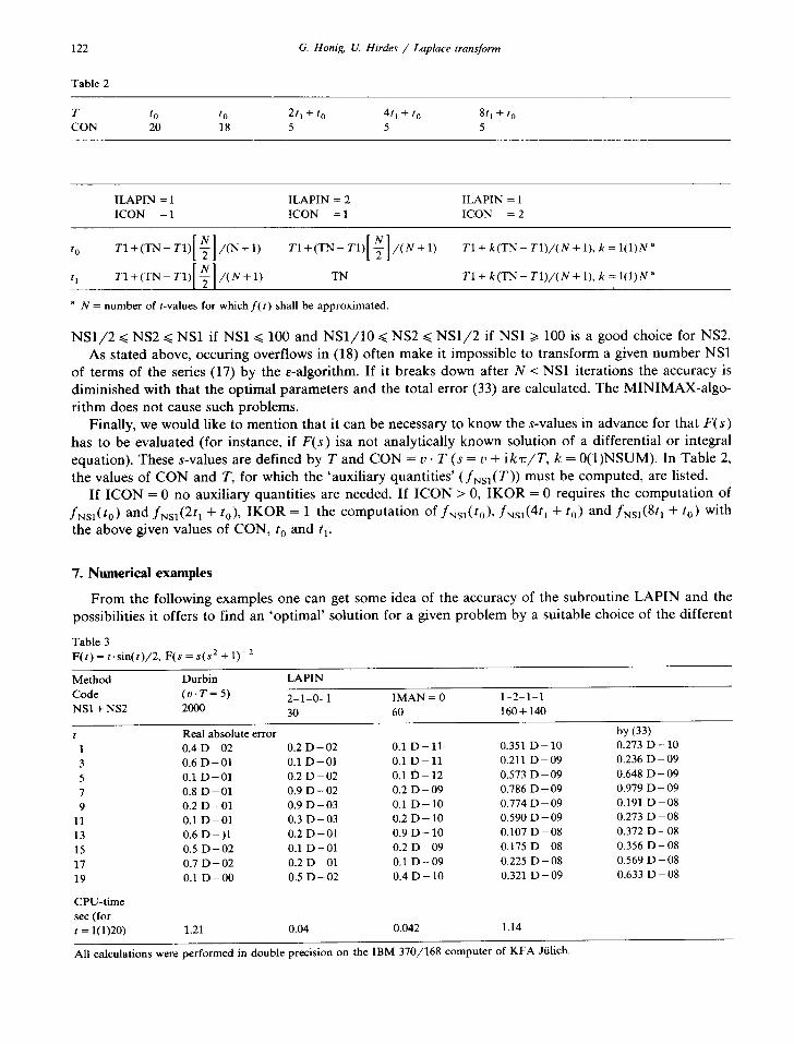
T a b l e 2

G. Honig, U. Hirdes / Laplace transform

T t o t o 2 t I + t o 4 t l + t o 8t 1 + t o C O N 20 18 5 5 5

I L A P I N = 1 I L A P I N = 2 I L A P I N = 1

I C O N = 1 ! C O N = 1 I C O N = 2

t o T I + ( T N - T 1 ) [ N ] / ( N + I ) T I + ( T N - T 1 ) [ N ] / ( N + I ) T I + k ( T N - T 1 ) / ( N + I ) , k = I ( 1 ) N a

t I T I + ( T N - T 1 ) [ 2 ] / ( N + I ) T N T I + k ( T N - T 1 ) / ( N + I ) , k = I ( 1 ) N "

a N = n u m b e r o f t -va lues for w h i c h f ( t ) shal l be a p p r o x i m a t e d .

N S 1 / 2 ~< NS2 ~< NS1 if NS1 ~< 100 and NS 1 / 10 ~< NS2 ~< N S 1 / 2 if NS1 >~ 100 is a good choice for NS2. As stated above, occuring overflows in (18) often make it impossible to transform a given number NS1

of terms of the series (17) by the e-algorithm. If it breaks down after N < NS1 iterations the accuracy is diminished with that the optimal parameters and the total error (33) are calculated. The MINIMAX-algo- ri thm does not cause such problems.

Finally, we would like to mention that it can be necessary to know the s-values in advance for that F ( s )

has to be evaluated (for instance, if F ( s ) isa not analytically known solution of a differential or integral equation). These s-values are defined by T and CON = v . T (s = v + i k v / T , k = 0(1)NSUM). In Table 2, the values of CON and T, for which the 'auxiliary quantities' ( fNsl (T)) must be computed, are listed.

If ICON = 0 no auxiliary quantities are needed. If ICON > 0, I K O R = 0 requires the computation of fNsl(t0) and fNm(2ta + to), I K O R = 1 the computation of fNsl(t0), fNSl(4tl + t 0) and fym(8t l + to) with the above given values of CON, t o and q-

7. Numerical examples

From the following examples one can get some idea of the accuracy of the subroutine LAPIN and the possibilities it offers to find an 'opt imal ' solution for a given problem by a suitable choice of the different

T a b l e 3 F ( t ) = t.sin(t)/2, F ( s = s(s 2 + 1) - 2

M e t h o d D u r b i n L A P I N

C o d e ( v . T = 5) 2 - 1 - 0 - 1 I M A N = 0 1 - 2 - 1 - 1 N S 1 + N S 2 2000 30 60 160 + 140

t Rea l abso lu t e e r r o r b y (33) 1 0.4 D - 0 2 0.2 D - 0 2 0.1 D - 1 1 0.351 D - 1 0 0 .273 D - 1 0

3 0.6 D - 0 1 0.1 D - 0 1 0.1 D - 1 1 0.211 D - 0 9 0 .236 D - 0 9

5 0.1 D - 0 1 0.2 D - 0 2 0.1 D - 1 2 0.573 D - 0 9 0 .648 D - 0 9

7 0.8 D - 0 1 0.9 D - 0 2 0.2 D - 0 9 0 .786 D - 0 9 0 .979 D - 0 9

9 0.2 D - 0 1 0.9 D - 0 3 0.1 D - 1 0 0 .774 D - 0 9 0.191 D - 0 8

11 0.1 D - 0 1 0.3 D - 0 3 0.2 D - 1 0 0 .590 D - 0 9 0.273 D - 0 8

13 0.6 D - ) 1 0.2 D - 01 0.9 D - 1 0 0 .107 D - 0 8 0 .372 D - 08

15 0.5 D - 0 2 0.1 D - 0 1 0.2 D - 0 9 0.175 D - 0 8 0 .356 D - 0 8

17 0.7 D - 0 2 0.2 D - 0 1 0.1 D - 0 9 0.225 D - 0 8 0 .569 D - 0 8

19 0.1 D - 0 0 0.5 D - 0 2 0.4 D - 1 0 0.321 D - 0 9 0.633 D - 0 8

C P U - t i m e

sec ( for t = 1(1)20) 1.21 0.04 0 .042 1.14

Al l ca l cu l a t i ons were p e r f o r m e d in d o u b l e p rec i s ion o n the I B M 3 7 0 / 1 6 8 c o m p u t e r o f K F A Jiilich.

G. Honig, U. Hirdes / Laplace transform 123

algorithms described above. The parameters used in the following tables are defined in Section 6. The code numbers refer to the parameters I L A P I N - I C O N - I K O R - I K O N V ( 1 - 2 - 0 - 1 , for example, means: ILAPIN = 1, ICON = 2, IKOR = 0 and IKONV = 1). IMAN = 0 coincides with 1 - 1 - 0 - 2 .

Table 3 shows the errors occuring if F(s)= s(s 2 + 1)-2 is inverted. Three different parameter combina- tions of LAPIN are compared with the method of Durbin. With only a few function evaluations of F(s) and little CPU-time, LAPIN computes the Laplace inverse with a considerable accuracy. For instance, the first two columns show that the method of Durbin needs about 60 times more function evaluations and 30 times more CPU-time than LAPIN to get a comparable accuracy. Column 3 shows--and this was confirmed by many other examples--that using the subroutine LAPIN as a 'black box' ( IMAN = 0) yields excellent results. From a comparison between columns 5 and 6 it is obvious that the absolute error computed by (33) is a good approximation for the real error (such an error estimation is only possible if ICON = 2; it is most accurate for IKONV = 1).

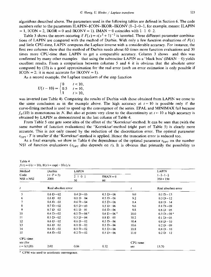
As a second example, the Laplace transform of the step function

0 t < l O , U(t- 10),= 0.5 t = 10,

1 t > 1 0 ,

was inverted (see Table 4). Comparing the results of Durbin with those obtained from LAPIN we come to the same conclusion as in the example above. The high accuracy at t = 10 is possible only if the curve-fitting method is used to speed up the convergence of the series. EPAL and MINIMAX fail because fN(10) is monotonous in N. But also at points very close to the discontinuity at t = 10 a high accuracy is obtained by LAPIN as demonstrated in the last column of Table 4.

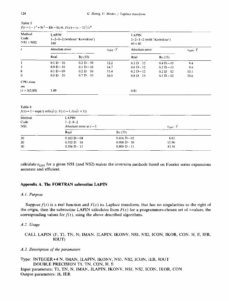
From Table 5 one gets some idea of the effect of the 'Korrektur'-method. It can be seen that (with the same number of function evaluations) the 'Korrektur '-method (right part of Table 5) is clearly more accurate. This is not only caused by the reduction of the discretization error. The optimal parameter roy r • T is smaller if the ' Korrektur'-method is applied. Hence the truncation error is reduced too.

As a final example, we show in Table 6 the dependence of the optimal parameter Vov r on the number NS1 of function evaluations (Oov r also depends on t). It is obvious that primarily the possibility to

Tab l e 4 f ( t ) = U(t - 10), F ( s ) = exp( - lOs) / s

Method D u r b i n L A P I N L A P I N

C o d e ( v . T = 5) 2 - 1 - 0 - 1 1MAN = 0 1 - 2 - 1 - 2 NS1 + NS2 2000 50 60 350 + 150

t Real absolute er ror t Real absolute er ror

5 0.6 D - 0 2 0.4 D - 0 5 0.5 D - 0 6 9.0 0.1 D - 1 3

6 0.6 D - 0 2 0.1 D - 0 4 0.5 D - 0 6 9.2 0.3 D - 1 2

7 0.6 D - 0 2 0.6 D - 0 4 0.5 D - 0 6 9.4 0.8 D - 1 4

8 0.7 D - 0 2 0.5 D - 0 3 0.5 D - 0 6 9.6 0.1 D - 0 9

9 0.7 D - 02 0.1 D - 01 0.6 D - 06 9.8 0.6 D - 05

10 0.6 D - 02 0.5 D - 04 a 0.6 D - 06 a 10.0 0.3 D - 09 a

11 0.5 D - 0 2 0.3 D - 0 4 0.8 D - 0 5 10.2 0.1 D - 0 5

12 0.6 D - 0 2 0.6 D - 0 2 0.5 D - 0 6 10.4 0.8 D - 1 0

13 0.6 D - 0 2 0.1 D - 0 2 0.5 D - 0 6 10.6 0.2 D - 0 9

14 0.6 D - 0 2 0.1 D - 0 2 0.5 D - 0 6 10.8 0.8 D - 1 0

15 0.6 D - 0 2 0.2 D - 0 2 0.5 D - 0 6 11.0 0.2 D - 1 2

C P U - t i m e

sec (for C P U - t i m e

t = 1(1)20) 2.02 0.06 0.32 sec 13.70

a C F M was used to accelerate convergence.

124 G. Honig, U. Hirdes / Laplace transform

Table 5 f ( t = ( - t 3 + 9t 2 - 18t + 6)/6, F(s) = (s - 1)3/s 4

Method LAPIN LAPIN Code 1 - 2 - 0 - 2 (without ' Korrektur') 1 -2 -1 -2 (with "Korrektur') NS1 + NS2 100 60 + 40

t Absolute error Vop v - T Absolute error roy r • T

Real By (33) Real By (33)

1 0.1 D - 1 0 0.2 D - 1 0 12.2 0.3 D - 1 2 0.4 D - 1 5 9.4 3 0.9 D - 1 0 0.1 D - 1 0 14.7 0.6 D - 1 2 0.5 D - 1 3 9.9 6 0.1 D - 0 9 0.2 D - 1 0 15.4 0.2 D - 1 2 0.2 D - 1 2 10.1 0 0.5 D - 1 0 0.7 D - 1 0 16.0 0.8 D - 1 3 0.1 D - 1 2 10.6

CPU-time s e c

( t = 1(1)10) 1.49 0.81

Table 6 f ( t ) = 1 - exp ( t ) erfc(~/t); F(s) = 1/(sVrs + 1))

Method LAPIN Code 1 - 2 - 0 - 2 NS1 Absolute error at t = 1 Vop x . T

Real By (33)

10 0.103 D - 0 4 0.416 D - 0 5 6.61 20 0.352 D - 10 0.900 D - 1 0 11.96 30 0.356 D - 1 1 0.801 D - 1 1 13.16

c a l c u l a t e Vop T fo r a g i v e n N S 1 ( a n d N S 2 ) m a k e s the i n v e r s i o n m e t h o d s b a s e d o n F o u r i e r ser ies e x p a n s i o n s

a c c u r a t e a n d e f f i c ien t .

Appendix A. The F O R T R A N subroutine L A P I N

A.1. Purpose

S u p p o s e f ( t ) is a r ea l f u n c t i o n a n d F ( s ) i t s L a p l a c e t r a n s f o r m , t h a t h a s n o s i n g u l a r i t i e s to t he r i g h t of

t h e o r ig in , t h e n t h e s u b r o u t i n e L A P I N c a l c u l a t e s f r o m F ( s ) for a p r o g r a m m e r s - c h o s e n set o f t -va lues , t he

c o r r e s p o n d i n g v a l u e s fo r f ( t ) , u s i n g t he a b o v e d e s c r i b e d a l g o r i t h m s .

A.2. Usage

C A L L L A P I N (F , T1 , T N , N , I M A N , I L A P I N , I K O N V , NS1 , NS2 , I C O N , I K O R , C O N , H, E, I E R ,

1 O U T )

A.3. Description o f the parameters

T y p e : I N T E G E R * 4 N , I M A N , I L A P I N , I K O N V , N S 1 , NS2 , I C O N , I E R , 1 O U T

D O U B L E P R E C I S I O N T1, T N , C O N , H, E

I n p u t p a r a m e t e r s : T1 , T N , N , I M A N , I L A P I N , I K O N V , N S 1 , NS2 , I C O N , 1 K O R , C O N

O u t p u t p a r a m e t e r s : H, I E R

G. Honig, U. Hirdes / Laplace transform 1 2 5

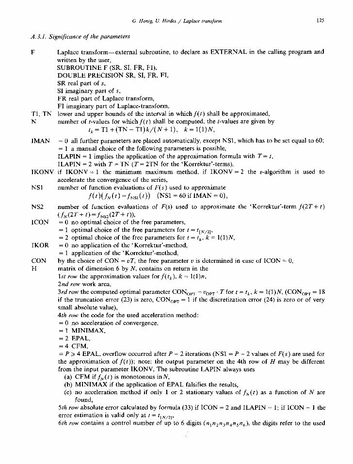
A. 3.1. Significance of the parameters

T1, TN N

I M A N

I K O N V

NS1

NS2

I C O N

I K O R

C O N H

Laplace t r ans fo rm--ex te rna l subroutine, to declare as E X T E R N A L in the calling program and written by the user, S U B R O U T I N E F (SR, SI, FR, FI), D O U B L E P R E C I S I O N SR, SI, FR, FI, SR real part of s, SI imaginary part of s, F R real part of Laplace transform, FI imaginary part of Laplace-transform, lower and upper bounds of the interval in which f ( t ) shall be approximated, number of t-values for which f ( t ) shall be computed, the t-values are given by

t k = T I + ( T N - T 1 ) k / ( N + I ) , k = l ( 1 ) N ,

= 0 all further parameters are placed automatically, except NS1, which has to be set equal to 60; = 1 a manual choice of the following parameters is possible, I L A P I N = 1 implies the application of the approximat ion formula with T = t, I L A P I N = 2 with T = T N (T = 2TN for the 'Korrektur ' - terms) , if I K O N V - 1 the m i n i m u m - m a x i m u m method, if I K O N V - - 2 the e-algorithm is used to accelerate the convergence of the series, number of function evaluations of F(s) used to approximate

f ( t ) ( f N ( t ) = f N s x ( t ) ) (NSa = 60 if I M A N = 0),

number of funct ion evaluations of F(s) used to approximate the 'Kor rek tur ' - t e rm f ( 2 T + t) ( f u (2T + t )= fNsz (2T+ t)), = 0 no opt imal choice of the free parameters, = 1 optimal choice of the free parameters for t = tiN~2], = 2 optimal choice of the free parameters for t = t k, k = 1(1)N, = 0 no application of the 'Korrek tur ' -method , = 1 application of the 'Korrek tur ' -method , by the choice of C O N = vT, the free parameter v is determined in case of I C O N = 0, matrix of dimension 6 by N, contains on return in the 1st row the approximat ion values for f ( tk) , k = l(1)n, 2nd row work area, 3rd row the computed optimal parameter C O N o v r = roy r • T for t = t k, k = I (1)N, ( C O N o v r = 18 if the truncation error (23) is zero, C O N o v r = 1 if the discretization error (24) is zero or of very small absolute value), 4th row the code for the used acceleration method: = 0 no acceleration of convergence, = 1 M I N I M A X , = 2 EPAL, = 4 CFM, = P >~ 4 EPAL, overflow occurred after P - 2 iterations (NS1 = P - 2 values of F(s) are used for the approximat ion of f ( t ) ) ; note: the output parameter on the 4th row of H may be different f rom the input parameter IKONV. The subroutine L A P I N always uses

(a) C F M i f f u ( t ) is monotonous inN, (b) M I N I M A X if the application of E P A L falsifies the results, (c) no acceleration method if only 1 or 2 stat ionary values of fN( t ) as a function of N are

found, 5th row absolute error calculated by formula (33) if I C O N = 2 and I L A P I N = 1; if I C O N = 1 the error estimation is valid only at t = tiN/21, 6th row contains a control number of up to 6 digits (n ln2n3nansn6) , the digits refer to the used

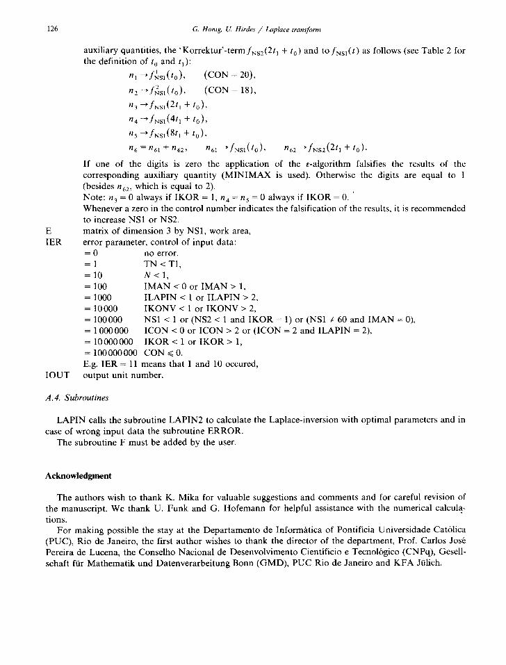
126 G. Honig, U. Hirdes / Laplace transform

E I E R

I O U T

auxiliary quantities, the definition of t o and t~):

n I ~ f r~s l ( t 0 ) , ( C O N = 20),

n 2 --)fN2s,(to), ( C O N = 18),

n 3 --)fNs,(2t, + to),

n 4 ~fNSa(4 t l + to),

the 'Korrek tur ' - t e rm fNS2 (2tl + t0) and to fNsl ( t ) as follows (see Table 2 for

n5 ----~fNS1 (8 t l q" 10),

n 6 = n61 -4- n62 , /-/61 --*fNsl(t0), n62 ~ f N s z ( 2 t l + to ) .

If one of the digits is zero the application of the e-algorithm falsifies the results of the corresponding auxiliary quanti ty ( M I N I M A X is used). Otherwise the digits are equal to 1 (besides n62 , which is equal to 2). Note: n 3 = 0 always if I K O R = 1, H a : n 5 = 0 always if I K O R = 0. Whenever a zero in the control number indicates the falsification of the results, it is recommended to increase NS1 or NS2. matrix of dimension 3 by NS1, work area, error parameter, control of input data: = 0 no error, = 1 T N < T1, = 1 0 N < I , = 100 I M A N < 0 or I M A N > 1, = 1000 I L A P I N < 1 or I L A P I N > 2, = 10 000 I K O N V < 1 or I K O N V > 2, = 100000 NS1 < 1 or (NS2 < 1 and I K O R = 1) or (NS1 4= 60 and I M A N = 0), = 1000 000 I C O N < 0 or I C O N > 2 or ( I C O N = 2 and I L A P I N = 2), = 1 0 0 0 0 0 0 0 I K O R < I o r I K O R > l , = 100000000 C O N ~< 0. E.g. I E R = 11 means that 1 and 10 occured, output unit number.

A. 4. Subroutines

L A P I N calls the subroutine L A P I N 2 to calculate the Laplace-inversion with optimal parameters and in case of wrong input data the subroutine E R R O R .

The subroutine F must be added by the user.

A c k n o w l e d g m e n t

The authors wish to thank K. Mika for valuable suggestions and comments and for careful revision of the manuscript . We thank U. Funk and G. H o f e m a n n for helpful assistance with the numerical calcula- tions.

For making possible the stay at the Depar tamento de Informhtica of Pontificia Universidade Cat61ica (PUC), Rio de Janeiro, the first author wishes to thank the director of the department, Prof. Carlos Jos6 Pereira de Lucena, the Conselho Nacional de Desenvolvimento Cientificio e Tecnolbgico (CNPq), Gesell- schaft for Mathemat ik und Datenverarbei tung Bonn (GMD), P U C Rio de Janeiro and K F A JiJlich.

G. Honig, U. Hirdes / Laplace transform 127

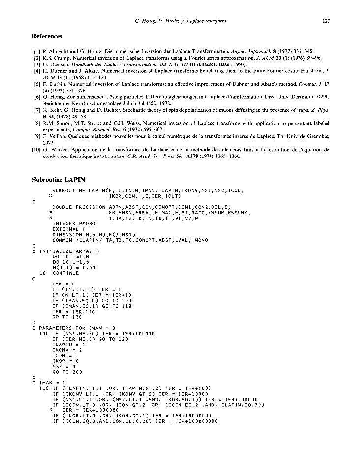
References

[1] P. Albrecht and G. Honig, Die numerische Inversion der Laplace-Transformierten, Angew. lnformatik 8 (1977) 336-345. [2] K.S. Crump, Numerical inversion of Laplace transforms using a Fourier series approximation, J. ACM 23 (1) (1976) 89-96. [3] G. Doetsch, Handbuch der Laplace-Transformation, Bd. L II, III (Birkh~iuser, Basel, 1950). [4] H. Dubner and J. Abate, Numerical inversion of Laplace transforms by relating them to the finite Fourier cosine transform, J.

ACM 15 (1) (1968) 115-123. [5] F. Durbin, Numerical inversion of Laplace transforms: an effective improvement of Dubner and Abate's method, Comput. J. 17

(4) (1973) 371-376. [6] G. Honig, Zur numerischen LOsung partieller Differentialgleichungen mit Laplace-Transformation, Diss. Univ. Dortmund D290,

Berichte der Kernforschungsanlage Jtilich-Jiil-1550, 1978. [7] K. Kehr, G. Honig and D. Richter, Stochastic theory of spin depolarization of muons diffusing in the presence of traps, Z. Phys.

B 32, (1978) 49-58. [8] R.M. Simon, M.T. Stroot and G.H. Weiss, Numerical inversion of Laplace transforms with application to percentage labeled

experiments, Comput. Biomed. Re{;. 6 (1972) 596-607. [9] F. Veillon, Quelques m6thodes nouvelles pour le calcul num+rique de la transform~ inverse de Laplace, Th. Univ. de Grenoble,

1972. [10] G. Warzee, Application de la transform~e de Laplace et de la m6thode des 61+ments finis ~ la r6solution de l'6quation de

conduction thermique instationnaire, C.R. Acad. Sei. Paris Sbr. A278 (1974) 1265-1266.

Subroutine LAPIN

SUBROUTINE LAPINCF,TI,TN,N, IMAN, ILAPIN, IKONV,NS1,NS2,1CON, x IKOR,CON,H,E, IER, IOUT)

DOUBLE PRECISION ABRN,ABSF,CON,CONOPT,CONI,CON2,DEL,E, x FN,FNSI,FREAL,FIMAGjH, PI,RACC,RNSUM, RNSUMK, x T,TA,TB,TK',TN,T0,TI,VI,V2,W INTEGER HMONO EXTERNAL F DIMENSION HC6,N),EC3,NSI) COMMON /CLAPIN/ TA,TB,T0,CONOPT,ABSF,LVAL,HMONO

INITIALIZE ARRAY H DO 10 I = I , N DO 10 J = l , 6 HCJ, I ) = 0.O0

10 CONTINUE

IER = 0 IF CTN.LT.T1) IER = 1 IF CN.LT . I ) IER = IER+I0 IF CIMAN.EQ.0) GO TO 100 IF CIMAN.EQ.I) GO TO 110 IER = IER+100 GO TO 120

PARAMETERS FOR IMAN = 0 100 IF CNSI.NE.60) IER : IER+I00000

IF CIER.NE.0) GO TO 120 ILAPIN = 1 IKONV = 2 ICON = 1 IKOR = 0 NS2 = 0 GO TO 200

IMAN = 1 110 IF CILAPIN.LT.1 .OR. ILAPIN.GT.2) IER = IER+I000

IF CIKONV.LT.1 .OR. IKONV.GT.2) IER = IER+10000 IF CNSI.LT. I .OR. CNS2.LT.1 .AND. IKOR.EQ.1)) IER = IF CICON.LT.0 .OR. ICON.GT.2 .OR. CICON.EQ.2 .AND.

:: IER = IER+1000000 IF CIKOR.LT.0 .OR. IKOR.GT.1) IER = IER+I00O0000 IF CICON.EQ.0.AND.CON.LE.0.D0) IER = IER+100OO0O00

IER+I00000 ILAPIN.EQ.2))

128 G. Honig, U. Hirdes / Laplace transform

IF (IER.EQ.0) GO TO 200 120 CALL ERROR(IER,T1,TN, N, IMAN, ILAPIN, IKONV,NSI,NS2,1CON, IKOR,

* CON, IOUT) RETURN

200 PI = 4.D0*DATAN(I.D0) CON1 = 20 .D0 CON2 = CON1-2 .D0 ABSF = 0 .D0

J3 = ( 3 - 1 C O N ) / 2 + N * ( I C O N / 2 ) TA = T I TB = TN

DO 830 L3=1,J3 LVAL = L3 HMONO = 0 KOR1 = IKOR

COMPUTATION OF THE OPTIMAL PARAMETERS 210 IF ( ICON- l ) 215,230,220 215 JUMP = 0

CALL LAPIN2(F,T1,TN,N, ILAPIN, IKONV,NSI,NS2,1CON, IKOR,CON,H,E,JUMP) GO TO 830

220 TA = TI+FLOAT(L3)*(TN-TI)/FLOAT(N+I) TB = TA

230 NH = N/2 T = T A + ( T B - T A ) * F L O A T ( N H ) / F L O A T ( N + I ) TK = F L O A T ( 2 - 1 L A P I N ) * T + F L O A T ( I L A P I N - I ) * T B

COMPUTATION OF THE TRUNCATION ERROR (RNSUM) TO = T CON = CONI JUMP = 1 CALL L A P I N 2 ( F , T I , T N , N , I L A P I N , I K O N V , N S 1 , N S 2 p l C O N p l K O R , C O N , H , E , J U M P )

240 FN : H ( I , L 3 ) FNS1 = E(1 ,NSI ) CON = CON2 JUMP : 2 CALL LAPIN2(F,TI,TN, N, ILAPIN, IKONV,NSI,NS2,1CON, IKOR,CON,H,E,JUMP)

250 IF (FN.NE.H(1,L3).AND.FNSI.NE.E(1,NS1)) GO TO 255 CONOPT = CON ABSF = 0.D0 GO TO 320

255 RNSUM = T K * ( F N - H ( I , L 3 ) ) / ( D E X P ( C O N I ) - D E X P ( C O N 2 ) ) IF ( I L A P I N . E Q . 2 ) GO TO 260

COMPUTATION OF THE ACCELERATION FACTOR ( D E L ) RACC = T * ( F N S 1 - E ( I , N S I ) ) / ( D E X P ( C O N I ) - D E X P ( C O N 2 ) ) DEL = RNSUM/RACC

260 IF (IKOR.EQ.1) GO TO 280

OPTIMAL PARAMETERS (METHOD A) TO = 2.D0*TK+T CON = CONI/4.D0 JUMP = 3 CALL LAPIN2(F,TI,TN,N, ILAPIN, IKONV,NSI,NS2,1CON, IKOR, CON,H,E,JUMP)

270 FN = H ( I , L 3 ) CONOPT = -TK/C2.D0*TK+T)*DLOG(DABS(RNSUM/(TK*FN))) GO TO 310

OPTIMAL PARAMETERS FOR THE KORREKTUR METHOD (METHOD A) 280 TO = 4 . D 0 * T K + T

CON = CON1/4 .D0 JUMP = 4 CALL L A P I N 2 ( F p T l p T N , N p l L A P I N , IKONVsNS1,NS2pICONplKORpCONpH, E, JUMP)

290 FN = H C 1 , L 3 ) TO = 8 . D 0 * T K + T JUMP = 5

G. Honig, U. Hirdes / Laplace transform 129

CALL LAPIN2(F,TI,TN,N, ILAPIN, IKONV,NSI,NS2,ICON, IKOR,CON,H,E,JUMP)

300 FN = FN-H(I,L3) CONOPT = -TK/(4.D0*TK+T)*DLOG(DABS(RNSUM/(TK*FN)))

C C OPTIMAL PARAMETERS (METHOD B)

310 IF (ILAPIN.EQ.1) GO TO 315 ABSF = DABS(DEXP(CONOPT)*RNSUM*2.DO/TK) GO TO 320

315 VI = CON1/T V2 = CONOPT/T W = PI*FLOAT(NSI)/T CALL F(V2,W,FREAL,FIMAG) RNSUMK = RNSUM*FREAL CALL F(VI,W,FREAL,FIMAG) RNSUMK = RNSUMK/FREAL ABRN = (RNSUMK-RNSUM)/(V2-V1) CONOPT = -DLOG(DABS((ABRN/T+RNSUMK)/(T*FLOAT(IKOR*2+2)*FN)))/

* F L O A T ( 3 + 2 * I K O R ) V l = V2 V2 = C O N O P T / T CALL F ( V 2 , W , F R E A L , F I M A G ) RNSUMK = R N S U M K * F R E A L CALL F ( V I , W , F R E A L , F I M A G ) RNSUMK = R N S U M K / F R E A L ABSF : D E X P ( C O N O P T ) / T : : D A B S ( R N S U M K ) +

* D A B S ( D E X P ( - 2 . D 0 * C O N O P T ) * F N * F L O A T ( I K O R - I ) * + D E X P C - 4 . D 0 * C O N O P T ) * F N * P L O A T ( I K O R ) )

C 320 IF ( C O N O P T . L E . 0 . D 0 ) CONOPT = I . D 0

JUMP = 6 CALL LAPIN2(F,TI,TN,N, ILAPIN, IKONV, NSI,NS2,1CON, IKOR, CON,H,E, JUMP)

830 CONTINUE RETURN END

SUBROUTINE LAPIN2(F,TI,TN,N, ILAPIN, IKONV,NSI,NS2, ICON, IKOR,CON, * H, E, JUMP)

C C LAPLACE-INVERSION WITH OPTIMAL PARAMETERS C

DOUBLE PRECISION A, ABSF,B,CON,CONOPT,DELTA,DIVI,E,EI,E2,E3,EINS, * FAKTOR,FIMAG,FREAL, H, PI,PIT, PITE,RAL,SUIM, SURE, * TA, TB, TE, TL, TM, TM1, TN, TT, T0, TI, XI, X2, X3, * V,W,YI,Y2,Y3 INTEGER RICHT, R ICHTA, HMONO EXTERNAL F DIMENSION H(6, N), E(3, NS1), E3 (3) COMMON /CLAPIN/ TA,TB,T0,CONOPT,ABSF,L3,HMONO

C PI = 4.DO*DATAN(I.D0)

C IF (JUMP.EQ.0) GO TO 360 IF (JUMP.LT.6) GO TO 370

C TO = TA TT = TB

11 : L3 J1 = (2-1CON)*N+(ICON-I)*L3 CON = CONOPT KOR1 = IKOR GO TO 380

C 360 TO = TI

TT -- TN I i = i J l = N KORI = IKOR JUMP : 6 GO TO 380

130 G. Honig~ U. Hirdes / Laplace transform

370 KOR1 = 0 TT = TO I i = L3 J1 = L3

C 380 DELTA = ( T T - T 0 ) / F L O A T ( N + I )

NSUM = NSl C C COMPUTATION OF THE T-VALUES FROM T 0 , T T

DO 805 K2=1,2 IF (ILAPIN.EQ.I) GO TO 420 TE : PLOAT(K2)*TT V = CON/TE CALL F(V,0.D0,PREAL,FIMAG) RAL = -0.SD0*PREAL PITE = PI/TE

C 405 DO 410 L=I,NSUM

W = FLOAT(L-1)*PITE CALL F(V,W,FREAL,FIMAG) E(2 ,L ) = FREAL E(3 ,L) = FIMAG

410 CONTINUE C

420 DO 800 K I= I1 ,J1 C

TL = T0+FLOAT(K1)*DELTA IF ( ILAPIN.EQ.2) GO TO 440

C IF (K2.EQ.2) TL = 3.D0*TL V = CON/TL FAKTOR = DEXP(V*TL)/TL CALL F(V,0.D0,FREAL,FIMAG) RAL = -0.5D0*FREAL PIT = PI/TL EINS = I.D0 SURE = 0.D0

C C METHOD OF DURBIN

425 DO 430 L=I,NSUM W = FLOAT(L-1)*PIT CALL F(V,W,FREAL,FIMAG) SURE = SURE+FREAL*EINS EINS = -EINS

E(I,L) = FAKTOR*(RAL+SURE) 430 CONTINUE

GO TO 460 C

440 IF (K2.EQ.2) TL = TL+TE FAKTOR = DEXP(V*TL)/TE SURE = 0.DO SUIM = 0.D0 DO 450 L=I,NSUM W = F L O A T ( L - I ) * P I T E SURE = S U R E + E ( 2 , L ) * D C O S ( W * T L ) SUIM = S U I M + E ( 3 , L ) * D S I N ( W * T L ) E ( I , L ) = FAKTOR* (RAL+SURE-SUIM)

450 CONTINUE C C SEARCH FOR STATIONARY VALUES

460 NMAX = NSUM*2/3 MONOTO = 0 K = 0 RICHTA = D S I G N ( 1 . S D 0 , ( E ( I , N S U M ) - E ( I , N S U M - I ) ) ) DO 500 L = I , N M A X J = NSUM-L RICHT = DSIGN(1.5D0,(E(I,J)-E(1,J-1))) IF (RICHT.EQ.RICHTA) GO TO 500 K = K+I E 3 ( K ) = E ( I , J ) RICHTA = RICHT IF ( K . E Q . 3 ) GO TO 510

G. Honig, U. Hirdes / Laplace transform 131

500 CONTINUE IF (K.EQ.0) GO TO 700 HCK2,K1) = ECI,NSUM) IF (K2.EQ.I) HC4,K1) = 0 GO TO 790

510 KE = 2 IF ((E3(KE)-E(1,J))::FLOAT(RICHTA).GT.0.D0) GO TO 560 JMIN = NSUM/3 JMAX = J-1 DO 540 JJ=JMIN, JMAX J = J-1 RICHT = DSIGN(I.5D0,(E(I,J)-E(1,J-1))) IF (RICHT.EQ.RICHTA) GO TO 540 RICHTA = RICHT KE - 3-KE IF ((E3(KE)-E(I,J));CFLOATCRICHTA).GT.0.D0) GO TO 560

54-0 CONTINUE 550 MONOTO = 1

IF (IKONV.EQ.2) GO TO 630 C C MINIMUM-MAXIMUM METHOD (MINIMAX)

560 H(K2,KI ) = (E3(1)+E3(3) ) /4 .D0+E3(2) /2 .D0 IF (K2.EQ.I) H(4,KI) = 1 GO TO 790

C C EPSILONALGORITHM (EPAL)

630 K : O NSUMMI = NSUM-1 E2 = E(I,I) DO 660 L=I,NSUMMI

El = E(I,I) TM = 0.D0 LP1 -- L+I DO 650 M=I,L MM = LP1-M TMI -- E(I,MM) DIVI -- E(I~MM+I)-E(I,MM) IF (DABS(DIVI).GT.I.D-20) GO TO 640 K = L GO TO 670

640 E(I,MM) = TM+I.DO/DIVI TM = TM i

650 CONTINUE E2 = E1

660 CONTINUE C

670 IF CDABSCEI).GT.DABSCE2)) El = E2 IF ( D A B S ( E C I , 1 ) ) . G T . D A B S ( E 1 ) ) E ( 1 , 1 ) = E1 H(K2,K1) : E(I,I) IF (K2.EQ.I) H(4,K1) = K+2 GO TO 790

C C CURVE FITTING (CFM)

700 Xl : FLOAT(NSUM)-2.DO X2 = FLOATCNSUM)-I.D0 X3 = FLOATCNSUM)-0.D0 Y1 = ECI,NSUM-2) Y2 = EC1,NSUM-1) Y3 = EC1,NSUM) B = ( (Y3-YI ) *X3*X3*CXl+X2) /CXl -X3)

x _(y2_y i )*X2,X2 xCxI+X3)/CxI_X2))/(X3_X2) A = ((Y2-YI)-B*(XI-X2)/(Xl*X2))*(X2*X2*XI*X1)/(XI*XI-X2*X2) H(K2,KI) = YI-(A/XI+B)/XI MONOTO = 1 IF (K2.EQ.1) HC4, K1) = 3

790 HC3,KI) = CON HC5,K1) = ABSF HMONO : HMONO+K2*MONOTO*I0**C6-JUMP) IF (JUMP.LT.6) GO TO 800 HC6,K1) = FLOATCC2-K2)*HMONO) +

132 G. Honig, U. Hirdes / Laplace transform

x F L O A T ( K 2 - 1 ) : : ( F L O A T ( 2 : : M O N O T O ) + H ( 6 , K 1 ) ) HMONO = H M O N O / 1 0 x I 0

800 CONTINUE IF (KORI .EQ.0) RETURN IF CK2.EQ.2) GO TO 810 NSUM = NS2

805 CONTINUE C C KORREKTUR METHOD

$I0 FAKTOR = -DEXP(-2.DOxCON) DO 820 K=II,JI H C I , K ) = H C I , K ) + F A K T O R X H ( 2 , K )

8 2 0 C O N T I N U E

RETURN END

SUBROUTINE ERRORCIER, TIpTN,N, IMAN, ILAPIN, IKONVpNS1,NS2,1CON, IKOR, :: CON, I O U T )

DOUBLE PRECISION T1,TN, CON

WRITE(IOUT, 1) IER, T I ,TN,N , IMAN, ILAPIN, IKONV,NSI,NS2,1CON, IKOR,CON 1 FORMATC///14H x:c:: ERROR =cx::,SXp5HIER =,I12//

x 10H T1 x ,D10.3 ,1BXp12HI ~¢ TN < T1/ :: 10H TN :: , D 1 0 . 3 / :: 10H N :: , I I 0 , 1 7 X , I I H I 0 :: N < I / :: 10H IMAN :: ~ I I 0 , 1 6 X , 2 9 H 1 0 0 :: IMAN < 0 OR IMAN > 1 / :: 1OH I L A P I N :: , I I 0 , 1 5 X , 3 4 H I 0 0 0 :: I L A P I N < i OR I L A P I N > 2 / :: 1OH IKONV :: 10H NS1

;: 10H NS2 ;'- 10H ICON

~: 10H IKOR :: 10H CON

RETURN END

x , I I 0 ,14Xs33H10000 x IKONV < 1 OR IKONV > 2/ :: , I10 ,13X,3BH100000 x NS1 < I OR CNS2 < i AND ,

41HIKOR = 1) OR CN$I <> 60 AND IMAN = 0 ) / x , 1 1 0 / x , I 10 ,12X,36H1000000 :: ICON < 0 OR ICON > 2 OR,

29H CICON = 2 AND ILAPIN = 2 ) / x , I10 ,11X,34H10000000 x IKOR < 0 OR IKOR > 1/ x ,D10.3,10X,21H1000000DD x CON <= 0 / / )