
ABA Banking Journal - October 2008 - Rethinking Segmentation
Journal of Banking and Finance 75 (2017) 258–279
Contents lists available at ScienceDirect
Journal of Banking and Finance
journal homepage: www.elsevier.com/locate/jbf
Modeling systemic risk and dependence structure between oil and
stock markets using a variational mode decomposition-based copula
method
Walid Mensi a , b , Shawkat Hammoudeh
c , d , ∗, Syed Jawad Hussain Shahzad
d , e , Muhammad Shahbaz
d
a Department of Finance and Accounting, University of Tunis El Manar, Tunis, Tunisia b Department of Finance and Investment, College of Economics and Administrative Sciences, Al Imam Mohammad Ibn Saud Islamic University (IMSIU),
P.O Box 5701 Riyadh, Saudi Arabia c Lebow College of Business, Drexel University, Philadelphia, United States d Energy and Sustainable Development (ESD), Montpellier Business School, Montpellier, France e COMSATS Institute of Information Technology, Islamabad, Pakistan
a r t i c l e i n f o
Article history:
Received 13 September 2016
Accepted 20 November 2016
Available online 23 November 2016
JEL classification:
C58
F37
G11
G14
Keywords:
Oil prices
Stock markets
Risk spillovers
Copula
Variational mode decomposition
Delta CoVaR
a b s t r a c t
This study combines the variational mode decomposition (VMD) method and static and time-varying
symmetric and asymmetric copula functions to examine the dependence structure between crude oil
prices and major regional developed stock markets (S&P50 0, stoxx60 0, DJPI and TSX indexes) during bear,
normal and bull markets under different investment horizons. Furthermore, it analyzes the upside and
downside short- and long-run risk spillovers between oil and stock markets by quantifying three market
risk measures, namely the value at risk (VaR), conditional VaR (CoVaR) and the delta CoVaR ( �CoVaR).
The results show that there is a tail dependence between oil and all stock markets for the raw return
series. By considering time horizons, we show that there is an average dependence between the con-
sidered markets for the short-run horizons. However, the tail dependence is also found for the long-run
horizons between the oil and stock markets, with the exception of the S&P500 index which exhibits aver-
age dependence with the oil market. Moreover, we find strong evidence of up and down risk asymmetric
spillovers from oil to stock markets and vice versa in the short-and long run horizons. Finally, the market
risk spillovers are asymmetric over the time and investment horizons.
© 2016 Elsevier B.V. All rights reserved.
p
f
c
t
u
p
a
b
h
c
u
1. Introduction
Oil is a strategic and vital commodity for all the economies of
the world. It underlies and interrelates to virtually every impor-
tant sector of the economy. For at least the last two decades, oil
prices have widely bounced up and down with varying passions
over relatively short periods of time. The oil roller coaster rides af-
fect businesses since oil serves as a fuel, as a feedstock and also
influences consumers through its effects on final demand because
this major energy source is used in transportation, home heat-
ing, services, etc. More recently, oil markets have been financial-
ized as a result of increasing exposure to different sets of market
∗ Corresponding author at: Lebow College of Business, Drexel University, Philadel-
phia, United States. Fax: + 1 2155714670.
E-mail addresses: [email protected] (W. Mensi),
[email protected] (S. Hammoudeh), [email protected] (S.J.H.
Shahzad), [email protected] (M. Shahbaz).
l
t
i
a
t
i
http://dx.doi.org/10.1016/j.jbankfin.2016.11.017
0378-4266/© 2016 Elsevier B.V. All rights reserved.
articipants including individual investors, money managers, hedge
unds, banks, insurance companies among others. The oil finan-
ialization has been helped by several financial tools such as op-
ions, futures, index funds, exchange traded funds, bespoke prod-
cts, etc. Investors use the oil asset to enhance returns, diversify
ortfolios and hedge against inflation since this fuel is considered
s a resource stock and a store of value. These characteristics have
rought oil markets closer to stock markets, and global forces also
ave increased their connectedness. Those markets have also come
loser to each other in the short run through the activity of spec-
lators and money managers.
That said, changes in oil prices play a significant role in the re-
ationship between oil and stock markets and have become one of
he important determinants of international stock markets’ volatil-
ty. Thus, investors’ decisions are based not only on the avail-
ble fundamental information in the stock markets but also on
he information prevailing in the oil markets. Therefore, examin-
ng the oil-stock market dependence is important for asset allo-

W. Mensi et al. / Journal of Banking and Finance 75 (2017) 258–279 259
c
d
t
o
c
p
a
i
t
e
i
o
B
c
e
M
t
i
k
s
t
k
h
d
a
f
w
b
d
d
t
r
l
V
M
u
m
r
c
f
r
i
c
e
k
a
C
t
r
u
s
t
(
r
(
f
q
n
t
l
s
c
g
t
u
l
s
m
r
e
a
u
c
a
v
f
(
(
f
d
s
m
o
r
p
S
h
t
r
s
s
i
n
m
m
k
T
i
t
a
2
S
e
i
r
S
2
ation and portfolio risk management. Given the oil intensity in
eveloped economies and the financialization of commodities in
hose economies, investors should be susceptible to the impact of
il price fluctuations on future equity returns. As expected dis-
ounted cash flows of any asset have the power to predict its
rice, 1 any factors altering these discounted cash flows can have
significant effect on these asset prices. Consequently, an increase
n oil prices may lead to a decrease in equity returns; however;
he status of the individual country being either an importer or an
xporter is of utmost importance for the oil-stock relationship. An
ncrease in oil prices exhibits a positive effect on the equity returns
f oil-exporting countries ( Jiménez-Rodríguez and Sanchez, 2005;
jørnland, 2009 ), whereas other studies argue that such an in-
rease in oil prices can result in a decrease in Dow Jones Stoxx600
quity returns of European countries ( Arouri and Nguyen, 2010 ). 2
oreover, the relationship between oil prices and stock market re-
urns varies across bear and bull market conditions due to hedg-
ng and herding among other reasons. Further, the oil-stock mar-
et dependence varies across investment time horizons (i.e., at
hort- and long-run investment horizons). Specifically, modeling
he evolving extreme dependence structure between these mar-
ets has important implications for financial risk management and
edging strategies.
Although there is a large body of the empirical literature that
eals with the oil-stock market comovements, little is known
bout how oil prices and stock markets co-move both during dif-
erent market conditions and at different investment horizons and
hat the upside and downside short- and long-run risk spillovers
etween them are. To discern the oil and stock co-movements at
ifferent investment horizons, we use an advanced multiresolution
ecomposition method, namely the variational mode decomposi-
ion (VMD), to decompose the original series into short- and long-
un components and capture the dependence in the upper and
ower tail distributions, using different specifications of copulas. 3
MD can decompose the non-stationary signal into couple Intrinsic
ode Functions adaptively and non-recursively ( Li et al., 2017 ). We
se a range of time-invariant, time-varying, symmetric and asym-
etric copula functions namely the Gaussian, Student-t, Gumbel,
otated Gumbel, Frank, Plackett, Clayton, rotated Clayton and SJC
opulas to compute the upside and downside spillover risk effects
rom crude oil to stock markets and vice versa for four major and
egional stock markets (i.e., the S&P500 index for the U.S., the TSX
ndex for Canada, the Stoxx600 for Europe and the Dow Jones Pa-
ific Stock Index excluding Japan for the Pacific basin) at differ-
nt investment horizons. We are also interested in regional mar-
et risks using three different risk measures which are the Value
t Risk (VaR), the Conditional Value at Risk (CoVaR) and the delta
onditional Value at Risk ( �CoVaR) to measure the risk spillovers.
Our choice of those four major stock markets is motivated by
heir respective regional locations (the United States, Canada, Eu-
ope and Pacific basin) and their relative global importance for eq-
ity and commodity markets. The Stoxx Europe600 index repre-
ents European stock markets, which are capitalized at $9.3 tril-
1 See Fisher (1930); Williams (1938) . 2 A negative relationship between oil price shocks and international equity re-
urns also is suggested by Jones and Kaul (1996), Sadorsky (1999) and Ciner
2001) for different countries. Jones and Kaul (1996) document that oil prices are a
isk factor for stock prices. However, studies by Chen et al. (1986) and Huang et al.
1996) do not support this negative association. 3 VMD has at least three advantages over the wavelet (Discrete Wavelet Trans-
orm) approach. (1) DWT is not as adaptive as the VMD technique, (2). DWT re-
uires a pre-determined wavelet function and a scale of decomposition, (3). The
umber of observations decreases with the level of decomposition, and this nega-
ively affects the linear estimates.
a
d
t
l
t
p
d
p
ion dollars in free-float market cap. 4 The TSX index, which is con-
idered as the benchmark for Canadian equities, is selected be-
ause Canada is a developed country with a clear resource oil and
as-based economy and a stock market capitalization of about $2
rillion. The S&P500 index is a major benchmark of the U.S. eq-
ity markets which have a market capitalization of about $22 tril-
ion. This index is also a major reference for international investors
ince it is considered as the most accurate gauge of the perfor-
ance of large-caps. Finally, the Dow Jones Pacific Stock Index is a
eference for the Pacific-Rim region.
To the best of the authors’ knowledge, no paper to date has: (i)
xamined the dependence structure between oil and stock markets
t different time investment horizons (short- and long-run) and
nder different market conditions (normal, bearish and bullish) by
ombining the VMD and copula methods; (ii) explored the upside
nd downside risk spillovers of oil markets to stock markets and
ice versa at short- and long-run investment horizons, using dif-
erent risk measures such as Value at VaR, CoVaR and delta CoVaR;
iii) tested if the up and down risk spillovers are asymmetric; and
iv) investigated whether the risk spillovers have asymmetric ef-
ects over the different time horizons for long and short positions.
The empirical results provide strong evidence of tail depen-
ence between oil and the considered major regional developed
tock markets for the raw return series. For the short-run invest-
ent horizons, we find an average positive dependence between
il and those four major developed stock markets. As for the long-
un investment horizons, we find asymmetric upper and lower de-
endence between those major markets as provided by the TVP
JC copula, with the exception of the U.S. stock market which ex-
ibits an average dependence with the oil market as detected by
he TVP Gaussian copula. On the other hand, we find significant
isk spillovers to the stock and to oil markets for the raw return
eries at both short- and long-run horizons.
More importantly, we find that the upside and downside risk
pillovers (from oil to stock markets and vice versa) are stronger
n the long-run than in the short-run for all cases. It also is worth
oting that the risk spillovers to oil are higher than those to stock
arkets. More interestingly, there is supportive evidence of asym-
etric upside and downside risk spillovers to stock and to oil mar-
ets for all cases in the short- and long-run investment horizons.
he downside and upside CoVaRs and �CoVaRs are asymmetric
n the short- and long-run for the oil and stock markets. Finally,
he impact of the onset of the GFC on risk spillovers is evident for
ll cases, as we find significant abrupt variations during the 2008–
009 crisis period.
The remainder of this paper is organized as follows.
ection 2 presents the literature review. Section 3 describes the
mpirical methods. Section 4 provides the data and some prelim-
nary statistics. Section 5 reports and discusses the empirical
esults. Section 6 presents the portfolio risk implications.
ection 7 draws policy implications and concludes the paper.
. Review of literature
A large body of the empirical literature has attempted to ex-
mine the intriguing links between oil and stock markets, using
ifferent econometric methods. In this review, we focus mostly on
he recent studies that are related to our methodology and markets
ocated in different regions but don’t provide a detailed review of
he old literature which is available in earlier studies.
Kling (1985) uses the vector autoregressive (VAR) model to ex-
lore the effects of oil prices on the S&P500 index and five U.S.
4 Source: STOXX Europe Total Market Index (TMI). https://www.stoxx.com/
ocument/Research/Expert- speak- articles/article _ european _ equity _ market _ 201502.
df

260 W. Mensi et al. / Journal of Banking and Finance 75 (2017) 258–279
(
k
r
fi
m
a
s
H
p
c
c
e
c
r
r
W
s
W
m
e
t
a
m
c
s
t
t
fi
a
c
i
i
e
o
t
r
s
R
b
a
l
i
p
o
p
t
i
a
i
I
a
n
b
u
s
f
h
t
s
industries. Chen et al., (1986) show that stock market returns are
exposed to systematic economic news. More interestingly, the au-
thors find no statistically significant relationship between oil price
and stock returns. Jones and Kaul (1996) use the current and future
changes in real cash flows and/or changes in expected returns to
explain the reaction of international stock markets (Canada, Japan,
UK and U.S.) to oil shocks. The authors demonstrate that the reac-
tion of the U.S. and Canadian stock prices to oil shocks can be com-
pletely accounted for by the impact of these shocks on real cash
flows alone. Huang et al., (1996) demonstrate that oil futures re-
turns lead some individual oil company stock returns but oil future
returns do not have much impact on broad-based market indices
as the S&P 500 index. Sadorsky (1999) uses the vector autoregres-
sion to determine how oil price movements play a crucial role to
explain a larger fraction of the forecast error variance in real stock
returns than interest rates do. Latter, Sadorsky (2012) uses the
multivariate GARCH model to analyze the correlations and volatil-
ity transmission between oil and the stock prices of clean energy
and technology companies. Mohanty et al., (2010) explore the con-
nection between oil prices and the stock returns of oil and gas
firms in Central and Eastern European (CEE) countries. The authors
find no significant linkages between oil prices and the stock re-
turns over the 1998–2010 period. Using a subperiod analysis, the
results show that oil price exposures of some oil and gas compa-
nies do vary across firms and over time. Vo (2011) investigates the
stock volatility-oil futures market linkages using the multivariate
stochastic volatility structure. The author finds that both markets
are inter-related and that the dynamic behavior increases when
the markets are more volatile. Balcilar and Ozdemir (2013) use
the Markov switching vector autoregressive (MS-VAR) model to
demonstrate that oil futures prices have strong regime prediction
power for subgroups of the S&P 500 stock index during different
subperiods in the sample. They find weak evidence for the regime
prediction power of a sub-grouping of the S&P 500 stock indexes.
Using the copula method, Aloui et al., (2013) provide evidence
of a contagion effect between oil and CEE transition economies
(Bulgaria, Czech Republic, Hungary, Poland, Romania and Slovenia).
In addition, the lower tail dependence is much stronger than that
of the upper tail. In contrast, Cong et al., (2008) apply the multi-
variate vector auto-regression and show no significant relationship
between oil price shocks and the real stock returns of most Chi-
nese stock sector indices, except for the manufacturing index and
some oil companies where important oil price shocks depress oil
company stock prices.
Du and He (2015) address the issue of extreme risk spillovers
between the S&P500 stock index and West Texas Intermediate
(WTI) crude oil futures returns, using the method of Granger
causality-in-risk, the Value at Risk (VaR) risk measure, and a
class of kernel-based tests to detect negative and positive risk
spillover effects. The results show strong evidence of significant
risk spillovers between the considered markets. Also, the authors
find that extreme movements in the oil market may have a signifi-
cant predictive power for those in the stock market and vice versa.
Using a Markov-Switching vector error-correction model, Balcilar
et al., (2015) examine the relationship between the U.S. crude oil
and stock market prices and find that the high-volatility regime
exists more frequently prior to the 1929 Great Depression and af-
ter the 1973 oil price shock engineered by the Organization of
Petroleum Exporting Countries (OPEC).
Kang et al. (2015) use a mixture innovation time-varying pa-
rameter VAR model to investigate the impact of structural oil price
shocks on the U.S. stock market returns and find evidence of time
variations in both the coefficients and the variance–covariance ma-
trix. Sim and Zhou (2015) examine the dependence between oil
prices and U.S. stock markets, using the quantile-on-quantile (QQ)
approach. These authors find that large, negative oil price shocks
or low oil price shock quantiles) can affect the U.S. stock mar-
et positively when this market is performing well (i.e., at high
eturn quantiles or during the bull stock markets). Moreover, they
nd that the dependence structure of oil prices on the U.S. stock
arket is asymmetric.
As for Ding et al. (2016) , the authors examine the causal link-
ges between the WTI and Dubai crude oil returns and five other
tock markets, including one in the U.S. and four in Asia (i.e., China,
ong Kong, Korea, and Japan), using the quantile causality ap-
roach. They find that the Nikkei and Hang Seng indices Granger-
ause the WTI returns. Moreover, all stock index returns Granger-
ause the Dubai crude oil returns over almost all quantile levels
xcept the Shanghai returns. The authors also show an asymmetric
ausality running from the Dubai crude oil returns to the Shanghai
eturns and from the Korean KOSPI returns to the Dubai crude oil
eturns.
Yang et al. (2016) examine the cross-correlations between the
TI crude oil and the ten sector stock markets in China. The re-
ults show that the strength of the multi-fractality between the
TI crude oil and the Chinese energy and financial sector stock
arkets is the highest, indicating a close connection between en-
rgy and financial markets. Furthermore, the authors use the vec-
or autoregression (VAR) method to analyze the interdependence
mong the multiple time series. The results reveal that the VAR
odel could not be used to describe the dynamics of the cross-
orrelations between the WTI crude oil and the ten Chinese stock
ectors.
Lu et al. (2016) consider a time-varying coefficient vector au-
oregressions (VAR) model to investigate the relationships between
he WTI crude oil and the U.S. S&P500 stock index. These authors
nd that the causal relations between oil and the U.S. stock market
re time- varying and display complex characters.
Liu et al. (2016) examine the dynamic spillovers between WTI
rude oil prices and two important stock markets (i.e., the S&P 500
ndex for the United States and the MICEX index for Russia). Apply-
ng a wavelet-based GARCH-BEKK method, the results show a pres-
nce of spillover effects between oil and the U.S. stock market and
il and the Russian stock market and that these effects vary across
he wavelet scales in terms of strength and direction. The spillover
elationship between oil and the U.S. stock market is shifting to the
hort-term, while the spillover relationship between oil and the
ussian stock market is changing to all time scales (daily, weekly,
imonthly and monthly), indicating that the linkage between oil
nd the U.S. stock market is weakening in the long-term, while the
inkage between oil and the Russian stock market is getting closer
n all time scales.
Raza et al. (2016) examine the asymmetric impact of gold
rices, oil prices and their associated volatilities on stock markets
f emerging economies, using the nonlinear ARDL (NARDL) ap-
roach. The results show that gold prices have a positive impact on
he stock market prices of emerging BRICS markets and a negative
mpact on the stock markets of Mexico, Malaysia, Thailand, Chile
nd Indonesia. Moreover, oil prices are found to have a negative
mpact on the stock markets of the emerging economies of China,
ndia, Brazil, Russia, South Africa, Mexico, Malaysia, Thailand, Chile,
nd Indonesia. On the other hand, gold and oil volatilities have a
egative impact on the stock markets of all emerging economies in
oth the short- and the long-run.
Our study complements the related literature since it deals with
p and down risk spillover effects and examines the dependence
tructure between oil and major regional stock markets during dif-
erent downturn, tranquil and upturn periods under diverse time
orizons (short- and long-run). The repercussions of the onset of
he GFC on the risk spillovers are also considered in this analy-
is. We also go beyond this analysis by investigating the potential

W. Mensi et al. / Journal of Banking and Finance 75 (2017) 258–279 261
a
f
3
3
m
c
a
n
t
u
�
ε
w
d
g
1
a
(
d
s
a
(
(
φ
w
β
i
a
l
w
p
G
d
w
a
s
a
G
c
3
d
c
t
b
d
F
w
f
s
o
c
t
i
t
o
f
w
a
s
d
o
j
l
m
o
λ
λ
w
t
s
w
d
v
T
F
z
e
a
t
i
w
t
t
d
e
S
w
2
ρ
w
f
p
�1
5 For an introduction on copulas, see Joe (1997) and Nelsen (2006) . For an
overview of copula applications to finance, see Cherubini et al. (2004) .
symmetric risk spillovers for long and short positions as well as
or short- and long-run.
. Methodology
.1. The marginal distribution model
To examine the dependence structure between oil and stock
arkets, we first estimate the marginal distributions of each finan-
ial time series using the ARFIMA-FIGARCH model which allows for
long range memory while keeping the residuals as standardized
ormal. The choice of this model is also supported by statistical
ests (see Section 4 ). The mean equation of the return series ( r t )
sing an ARFIMA ( m , d , n ) model can be expressed as follows:
( L ) ( 1 − L ) d ( y t − μ) = �( L ) ε t , (1)
t = z t √
h t , z t ∼ N ( 0 , 1 ) (2)
here ε t is the independently distributed error with variance h t ,
is the fractional difference parameter which measures the de-
ree of long memory, L denotes the lag operator, and �(L ) = − �1 L − �2 L
2 . . . − �m
L m and �(L ) = 1 + �1 L + �2 L 2 · · · + �n L
n
re, respectively, the autoregressive (AR) and the moving-average
MA) polynomials.
To be more specific, the ARFIMA process is non-stationary when
≥ 0 . 5 , and exhibits a LM for 0 < d < 0 . 5 . The process exhibits a
hort (intermediate) memory for d = 0 ( d < 0 . 5 ). It exhibits a neg-
tive dependence between distant observations if −0 . 5 < d < 0 . 5
anti-persistence).
We follow Baillie et al. (1996) by introducing the FIGARCH
p, ξ , q ) process as follows,
( L ) ( 1 − L ) ξ ε 2 t = ω + [ 1 − β( L ) ] V t , (3)
here φ(L ) ≡ φ1 L + φ2 L 2 + · · · + φq L
q , β(L ) ≡ β1 L + β2 L 2 + · · · +
p L p and V t ≡ ε 2 t − h t . The { V t } process can be interpreted as the
nnovation for the conditional variance, which has a zero mean
nd is serially uncorrelated. All the roots of φ(L ) and [ 1 − β(L ) ]
ie outside the unit root circle. We have a stationary LM process
hen 0 ≤ ξ ≤ 1 . If ξ = 1 , the process has a unit root, and thus a
ermanent shock effect.
In this paper, we consider the Student-t-distributions for the FI-
ARCH model. The Hansen (1994) skewed-t density distribution is
efined as follows.
f ( z t , v , η) =
⎧ ⎪ ⎨
⎪ ⎩
bc
(1 +
1 v −2
(b z t + a 1 −η
)2 )−( v +1 ) / 2
z t < −a/b
bc
(1 +
1 v −2
(b z t + a 1+ η
)2 )−( v +1 ) / 2
z t ≥ −a/b
(4)
here v and η are the degree of freedom parameters ( 2 < v ≤ ∞ )
nd the symmetric parameter ( −1 < η < 1 ) , respectively. The con-
tants a, b and c are given by:
= 4 ηc
(v − 2
v − 1
), b 2 = 1 + 3 η − a 2 , and
c = (v + 1
2
)/ √
π( v − 2 ) ( v
2
).
If n = 0 and v → ∞ , then the skew-t converges to the standard
aussian distribution, but if η = 0 and v is finite, then the skew-t
onverges to the symmetric Student-t distribution.
.2. Copula approach
This study uses bivariate copulas to model the average and tail
ependence between oil and stock markets. The cornerstone of the
opula theory is the Sklar’s theorem which states that a joint dis-
ribution F ( x , y ) of two continuous random variables X and Y can
XYe expressed in terms of a copula function C(u,v) and the marginal
istribution functions of the random variables, F X (x) , F Y (y) as
XY ( x , y ) = C ( u , v ) , (5)
here u = F X (x) and v = F Y (y) . Thus, a copula is a multivariate
unction with uniform marginals that represents the dependence
tructure between two random variables. It is uniquely determined
n Ran F X × Ran F Y when the margins are continuous. In terms of
onstruction, copulas can be used to connect marginals to a mul-
ivariate distribution function, which in turn can be decomposed
nto its univariate marginal distributions and a copula that cap-
ures the dependence structure. 5
The joint probability density of the variables X and Y can be
btained from the copula density, c( u , v ) =
∂ 2 C( u , v ) ∂ u ∂ v
, as
XY ( x , y ) = c ( u , v ) f Y ( y ) f x ( x ) , (6)
here f Y (y) and f x (x) denote the marginal densities of the vari-
bles Y and X, respectively. Hence, to characterize the joint den-
ity of two random variables, we need information on the marginal
ensities and on the copula density.
An appealing feature of a copula is that it provides information
n average dependence and on the probability that two variables
ointly experience extreme upward or downward movements. The
atter extreme dependence measure is called tail dependence. A
easure of the upper (right) and lower (left) tail dependence is
btained from the copulas as:
U = lim
u → 1 Pr
[X ≥ F −1
X ( u ) | Y ≥ F −1 Y ( u )
]= lim
u → 1
1 − 2u + C ( u , u )
1 − u
, (7)
L = lim
u → 0 Pr
[X ≤ F −1
X ( u ) | Y ≤ F −1 Y ( u )
]= lim
u → 0
C ( u , u )
u
, (8)
here λU , λL ∈ [ 0 , 1 ] . The lower (upper) tail dependence means
hat λL > 0 ( λU > 0 ), which indicates a non-zero probability of ob-
erving an extremely small (large) value for one series together
ith an extremely small (large) value for another series.
Our study uses a diverse family of copula specifications with
ifferent dependence structures and time-invariant and time-
arying parameters. Table 1 summarizes the copula specifications.
he symmetric copulas include the bivariate Normal copula, the
rank copula and the Plackett copula with tail independence (or
ero-tail dependence). They also include the Student-t copula with
qual lower and upper tail dependence. The asymmetric copulas
re the Gumbel copula with an upper tail dependence and lower
ail independence, the rotated Gumbel copula with an upper tail
ndependence and a lower tail dependence, the Clayton copula
ith an upper tail independence and a lower tail dependence, and
he symmetrized Joe–Clayton copula (SJC) with a special case of
he symmetric tail dependence.
For all the above copula functions, we model the time-varying
ependence by allowing the copula dependence parameter to
volve according to an evolution equation. For the Gaussian and
tudent-t copulas, we specify the linear dependence parameter ρt
hich evolves according to an ARMA(1,q)-type process (see Patton,
006 ):
t = �
(
�0 + �1 ρt −1 + �2 1
q
q ∑
j=1
�−1 (u t −j
). �−1
(v t −j
))
, (9)
here �(x) = ( 1 − e −x ) ( 1 + e −x ) −1 is the modified logistic trans-
ormation to keep the value of ρt in ( −1,1). Hence, the dependence
arameter is explained by a constant �0 , by an autoregressive term
, and by the average product over the last q observations of the

262 W. Mensi et al. / Journal of Banking and Finance 75 (2017) 258–279
Ta
ble 1
Biv
ari
ate co
pu
la fu
nct
ion
s.
Co
pu
la N
am
e
Form
ula
Pa
ram
ete
r T
ail d
ep
en
de
nce
No
rma
l (N
) C N
( u ,
v , ρ)
= �
( �−1
(u) , �
−1
(v) )
ρ∈
[ −1 1 ]
Ze
ro ta
il d
ep
en
de
nce
: λ
L =
λU
= 0
Stu
de
nt-
t (t
) C S
T
( u ,
v , ρ
, υ
) =
T( t −1
υ( u
) , t −
1
υ( v
) )
ρ∈
[ −1 1 ]
Sy
mm
etr
ic ta
il d
ep
en
de
nce
: λ
U
= λ
L =
2 t υ
+1
( −√ υ
+ 1 √ 1
−
ρ/ √ 1
+
ρ)
> 0
Cla
yto
n (C
L)
C C
L ( u ,
v ;δ
) =
ma
x { ( u
−δ+
v −δ
−1 ) −1
/δ
, 0 }
α∈
[ −1 ,
∞ ) \{
0 }
Asy
mm
etr
ic ta
il d
ep
en
de
nce
: λ
L =
2 −1 /δ,
λU
= 0
Gu
mb
el
(Gu
) C G
( u ,
v ;δ
) =
ex
p ( −
( ( −l
og u ) δ
+ ( −
log v ) δ
) 1 /δ)
δ∈
[ 1 ,
∞ )
Asy
mm
etr
ic ta
il d
ep
en
de
nce λ
L =
0 ,
λU
= 2 −
2 1 /δ
Ro
tate
d G
um
be
l C R
G
( u ,
v ;δ
) =
u +
v −
1 +
C G
( 1 −
u ,
1 −
v ;δ
) 0 <δ< ∞
Up
pe
r ta
il in
de
pe
nd
en
ce a
nd lo
we
r ta
il d
ep
en
de
nce
Fra
nk (F
) C F
( u ,
v ;δ
) =
δlo
g ( [ ( 1 −
e −δ
) −
( 1 −
e −δ
u
)( 1 −
e −δ
v
) ] / ( 1 −
e −δ
) )
θZ
ero ta
il d
ep
en
de
nce
: λ
L =
λU
= 0
Pla
cke
t C P
( u ,
v ;θ
) =
1
2( θ
−1 ) ( 1 +
( θ−
1 )( u +
v ) ) −
√ ( 1 +
( θ−
1 )( u +
v ) ) 2
−4 θ( θ
−1 ) u
v
λL
∈ ( 0 ,
1 )
Ze
ro ta
il d
ep
en
de
nce
: λ
L =
λU
= 0
SJC
C S
JC
( u ,
v ;λ
U
, λ
L )
= 0 . 5
( C JC
( u ,
v ;λ
U
, λ
L ) +
C JC
( 1 −
u ,
1 −
v ;λ
U
, λ
L ) +
u +
v −
1 )
λU
∈ ( 0 ,
1 )
λU
= λ
L
Joe C
lay
ton
C JC
( u ,
v ;λ
U
, λ
L )
= 1 −
( 1 −
{ [ 1 −
( 1 −
u ) k
] −γ+
[ 1 −
( 1 −
v ) k
] −γ−
1 } −1
/γ
) 1 / k
λL
∈ ( 0 ,
1 )
λU
t =
�( ω
U
+ β
U
ρt −
1
+ α
U
1
q
q ∑ j=1
| u t −j
−v t −
j | )
λU
∈ ( 0 ,
1 )
λL t
= �
( ω L
+ β
L ρ
t −1
+ α
L 1
q
q ∑ j=1
| u t −j
−v t −
j | )
No
tes: λ
L a
nd
λU
de
no
te th
e lo
we
r a
nd u
pp
er
tail d
ep
en
de
nce
, re
spe
ctiv
ely
. Fo
r th
e N
orm
al
cop
ula
, �
−1
(u)
an
d �
−1
(v)
are th
e st
an
da
rd n
orm
al
qu
an
tile fu
nct
ion
s a
nd �
is th
e b
iva
ria
te st
an
da
rd n
orm
al
cum
ula
tiv
e d
istr
ibu
tio
n fu
nct
ion w
ith co
rre
lati
on
ρ.
For
the S
tud
en
t-t
cop
ula
, t −
1
υ(u
) a
nd t −
1
υ(v
) a
re th
e q
ua
nti
le fu
nct
ion
s o
f th
e u
niv
ari
ate S
tud
en
t-t
dis
trib
uti
on w
ith υ
as
the d
eg
ree
-of-
fre
ed
om p
ara
me
ter
an
d T is th
e b
iva
ria
te S
tud
en
t-t
cum
ula
tiv
e d
istr
ibu
tio
n fu
nct
ion w
ith
υa
s th
e d
eg
ree
-of-
fre
ed
om p
ara
me
ter
an
d ρ
as
the co
rre
lati
on
. Fo
r th
e S
JC co
pu
la, κ
= 1 / lo
g 2
(2 −
λU
) , γ
= −1
/ lo
g 2
( λL ) .
t
t
t
u
a
δ
e
λ
λ
w
r
i
3
i
a
m
p
w
t
e
s
e
b
c
G
a
a
m
w
b
r
r
a
r
m
s
o
L
w
s
v
ransformed variables, �2 . For the Student-t copula, the parame-
er dynamics are also given by Eq. (9) by substituting �−1 (x) by
−1 υ (x) . The dynamics of the Gumbel and the rotated Gumbel cop-
las are assumed to follow the ARMA(1,q) process that is specified
s
t = ω + βδt −1 + α1
q
q ∑
j=1
∣∣u t −j − v t −j
∣∣. (10)
Finally, for the SJC copula, the tail dependence parameters
volve according to:
U t = �
(
ω U + βU ρt −1 + αU 1
q
q ∑
j=1
∣∣u t −j − v t −j
∣∣)
, (11)
L t = �
(
ω L + βL ρt −1 + αL 1
q
q ∑
j=1
∣∣u t −j − v t −j
∣∣)
, (12)
here �(x) = ( 1 + e −x ) −1 is the logistic transformation used to
etain λU t and λL
t in (0,1).
The main characteristics of the bivariate copula functions used
n this study are summarized in Table 1.
.3. Variational mode decomposition (VMD)
The fundamental concept of VMD decomposes a time series f
nto a discrete k number of sub-series (known as modes) u k ,
nd the bandwidth of each mode is limited in the spectral do-
ain. Each decomposed variational mode k is assumed to be com-
ressed around a center pulsation, ω k , which is determined along
ith the decomposition. The determination of the algorithm of
he bandwidth of a time series requires: (i) obtaining a unilat-
ral frequency spectrum for each mode u k by computing the as-
ociated analytic signal by means of the Hilbert transform; (ii) for
ach mode, shifting the mode’s frequency spectrum to a baseband
y mixing with an exponential tuned to the respective estimated
enter frequency; and (iii) estimating the bandwidth through the
aussian smoothness of the demodulated signal ( Dragomiretskiy
nd Zosso, 2014 ).
Thus, the resulting constrained variational problem can be given
s:
i n { u k } , { ω k } =
{ ∑
k
∥∥∥∥∂ t
[(δ( t ) +
j
πt
)∗ u k ( t )
]e − j ω k t
∥∥∥∥2
2
}
s.t ∑
k
u k = f (13)
here ∂ t denotes the partial derivatives, k indicates the set (num-
er) of modes u of the original signal f while ω, δ(t) and
∗ rep-
esent the frequency, the Dirac distribution and the convolution,
espectively. Thus, { u k } := { u 1 , . . . .. u k } and { ω k } := { ω 1 , . . . . ω k } re the sets of all variational modes and their central frequency,
espectively. Eq. (13) decomposes the original signal into a set of
odes ( k ) with a limited bandwidth in the Fourier domain. The
olution to the original minimization problem is the saddle point
f the following augmented Lagrange ( L ) expression:
( u k , ω k , λ) = α∑
k
∥∥∥∥∂ t
[(δ( t ) +
j
πt
)∗ u k ( t )
]∥∥∥∥2
2
+
∥∥∥ f −∑
u k
∥∥∥2
2 +
⟨ λ, f −
∑
u k
⟩ (14)
here α denotes the balancing parameter of the data-fidelity con-
traint, λ is the Lagrange multiplier and ‖ � ‖ p denotes the usual
ector � p norm where p = 2 . The solution to Eq. (14) is found in a

W. Mensi et al. / Journal of Banking and Finance 75 (2017) 258–279 263
s
u
u
ω
a
λ
u
o
i
(
3
f
V
m
l
s
i
t
a
r
A
t
l
t
c
s
F
a
n
o
d
m
a
P
w
a
r
t
i
P
w
s
h
o
m
b
i
C
1
w
o
c
v
a
f
a
E
F
E
m
t
d
m
s
b
�
�
k
s
v
t
t
I
K
w
t
t
b
4
W
p
d
c
I
2
f
B
E
b
1
fi
r
t
6 The Dow Jones Pacific Stock Index is a capitalization-weighted index comprised
of companies traded publicly in selected countries located in the Pacific-Rim region
excluding Japan. It is calculated in US dollars.
equence of k iterative sub-optimizations. Finally, the solutions for
and ω are found in the Fourier domain and are given by
n +1 k
=
(
f −∑
i � = k u i +
λ
2
)
1
1 + 2 α( ω − ω k ) 2
(15)
n +1 k
=
∫ ∞
0 ω | u k ( ω ) | 2 d ω ∫ ∞
0 | u k ( ω ) | 2 d ω (16)
nd for λ it’s updated as
ˆ n +1 ←
ˆ λn + τ
(
ˆ f −∑
k
ˆ u
n +1 k
)
(17)
ntil convergence: ∑
k ‖ ̂ u n +1 k
− ˆ u n k ‖ 2
2 / ‖ ̂ u n
k ‖ 2
2 , where k is the number
f iterations. We set the number of modes k to ten. It is worth not-
ng that the sum of VMD components equals to the original signal
see Dragomiretskiy and Zosso, 2014 ).
.4. VaRs, CoVaRs and delta CoVaRs risk measures
We quantify both the downside and upside VaRs and CoVaRs
or the oil and stock market returns using the copula results. The
aR risk measure quantifies the maximum loss that an investor
ay incur within a specific time horizon and with a confidence
evel by holding a long position (i.e., downside risk) or a short po-
ition (i.e., upside risk).
The downside VaR at time t and for a confidence level 1 − αs expressed by P r( r t ≤ V a R α,t ) = α, which can be computed from
he marginal models as V a R α,t = μt + t −1 υ,η(α) σt , where μt and σt
re the conditional mean and standard deviation of the return se-
ies, computed according to mean and variance equation of the
RFIMA-FIGARCH model ( Eqs. (1) –( 3 )), and where t −1 υ,η(α) denotes
he α quantile of the skewed Student-t distribution in Eq. (4) . Simi-
arly, the upside VaR is given by considering P r( r t ≥ V a R 1 −α,t ) = α;
hus the upside VaR is given by V a R 1 −α,t = μt + t −1 υ,η( 1 − α) σt .
Given the strong linkages between oil and stock markets, we
onsider the impact of financial distress in the oil market, as mea-
ured by its VaR, on the VaR of the stock market and vice versa.
or a deeper analysis, we study CoVaR that is developed by Adrian
nd Brunnermeier (2011) and Girardi and Ergün (2013) . As a defi-
ition, the CoVaR for the asset i is the VaR for asset i conditional
n the fact that asset j exhibits an extreme movement.
Let r s t be the returns for stock and r o t be the returns for oil. The
ownside CoVaR for stock returns for an extreme downward oil
ovement and a confidence level 1 − β can be formally expressed
s the β-quantile of the conditional distribution of r s t as:
r (r s t ≤ CoV aR
s β,t | r o t ≤ V aR
o α,t
)= β (18)
here V aR o α,t is the α-quantile of the oil price return distribution
nd Pr ( r o t ≤ V aR o α,t ) = α measures the maximum loss that oil price
eturns may experience for a confidence level 1 − α and a specific
ime horizon.
Similarly, the upside CoVaR for an extreme upward movement
n oil price returns:
r (r s t ≥ CoV aR
s β,t | r o t ≥ V aR
o 1 −α,t
)= β, (19)
here V aR o 1 −α,t
quantifies the maximum loss by considering a
hort position for a confidence level 1 − α and for a specific time
orizon.
Interestingly, we can measure the systemic impact of a stock on
il by considering the CoVaR for the oil market instead of the stock
arket as in Eqs. (18) and ( 19 ). The CoVaR in those equations can
e represented in terms of copulas, since the conditional probabil-
ties can be re-written, respectively, as:
(F r s t
(CoV aR
s β,t
), F r o t
(V aR
o α,t
))= αβ (20)
− F r s t
(CoV aR
s β,t
)− F r o t
(V aR
o 1 −α,t
)+ C
(F r s t
(CoV aR
s β,t
), F r o t
(V aR
o 1 −α,t
))= αβ, (21)
here F r s t and F r o t
are the marginal distributions of the stock and
il returns, respectively. We follow Reboredo and Ugolini (2015) to
ompute the CoVaR by following a two-step procedure.
In step 1, we can solve Eq. (20) or (21) in order to obtain the
alue of F r s t ( CoV aR s
β,t ) , given the significance levels for the VaR
nd CoVaR and β respectively, and for specific forms of the copula
unction. In step 2, we use the distribution function for the oil
nd stock market returns as given by the marginal model in
qs. (1) –( 3 ) and compute the CoVaR for stock as
−1 r s t
( F r s t ( CoV aR s
β,t ) ) .
We follow Adrian and Brunnermeier (2011) and Girardi and
rgün (2013) to define the systemic risk contribution of a stock
arket s as the delta CoV aR ( � CoV aR ), which is the difference be-
ween the V aR of the stock market as a whole conditional on the
istressed state of market s ( R s t ≤ V aR s α,t ) and the V aR of the stock
arket as a whole conditional on the benchmark state of market
, considering it as the median of the return distribution of market
s , or, alternatively, the V aR for α = 0 . 5 . The systemic risk contri-
ution of market s is thus defined as:
C oV aR
s/o t =
(C oV aR
s/o
β,t − C oV aR
s/o, α=0 . 5
β,t
)C oV aR
s/o,α=0 . 5
β,t
(22)
CoV aR is useful as it captures the marginal contribution of mar-
et s to the overall systemic risk.
We test for the significance of systemic risk using the KS boot-
trapping test developed by Abadie (2002) to compare the CoVaR
alues. The KS test measures the difference between two cumula-
ive quantile functions relying on the empirical distribution func-
ion but without considering any underlying distribution function.
t is defined as:
S mn =
(mn
m + n
) 1 l
sup
x | F m
( x ) − G n ( x ) | , (23)
here F m
(x ) and G n (x ) are the cumulative CoVaR and VaR dis-
ribution functions, respectively, and n and m are the sizes of the
wo samples. Thus, we test the hypothesis of no systemic impact
etween stock and oil markets as: H 0 : CoV aR s β,t
= V aR s β,t
.
. Data and descriptive statistics
Our analysis is based on the daily closing spot prices for the
TI crude oil, which is a global benchmark for determining the
rices of other light crudes in the United States, and four regional
eveloped stock markets (i.e., S&P500, stoxx600, Dow Jones Pa-
ific Stock Index and TSX-Toronto Stock Exchange 300 Composite
ndex). 6 The study spans the period from June 4, 1998 to May 6,
016. The data for S&P50 0, Stoxx60 0 and TSX indexes are sourced
rom Datastream, while for the DJPS index it is obtained from
loomberg. The data for the WTI oil price is obtained from the US
nergy Information Administration. The sample period is marked
y several extreme events and turbulences including the 1997–
998 Asian crisis, the 2001 dot-com bubble, the 20 07–20 09 global
nancial crisis and the 2009–2012 euro-zone debt crisis. This pe-
iod is also characterized by higher volatility of the oil price.
Fig. 1 illustrates the trajectory of the daily level series over
he sample period. This figure displays a spectacular rise in the

264 W. Mensi et al. / Journal of Banking and Finance 75 (2017) 258–279
Fig. 1. Time-variations of daily WTI crude oil prices and the four major developed stock indexes.
Fig. 2. The WTI crude oil price returns and major developed stock index returns dynamics.
s
t
u
i
s
k
t
t
l
S
risk.
oil price in 2008 where the price of a barrel of crude oil ex-
ceeds US$140/barrel in July 2008, while it shows a significant de-
cline for most of the period dating back to 2015 during which the
oil price remains under US $50 a barrel. The continuously com-
pounded daily returns are computed by taking the difference in
the logarithm of two consecutive prices. Fig. 2 depicts the evolu-
tion dynamics of the return series and illustrates the stylized facts
(e.g., volatility clustering) for the oil and the four major stock index
return series.
Table 2 presents the descriptive statistics of the oil price returns
and the four regional developed index returns between May 1998
and May 2016. The average return series are positive for all the
eries. More precisely, oil and DJPI hold the highest average re-
urns, while stoxx 600 index has the lowest average returns. The
nconditional volatility is similar across the four stock markets. Oil
s more volatile than those stock markets. The negative values for
kewness are common for all the series, which also exhibit excess
urtosis. The Jarque–Bera test rejects the null of Gaussian distribu-
ion for all the series. DJPI has the highest Sharp ratio, indicating
he most rewarding investment, while the stoxx600 index has the
owest ratio and thus is the least rewarding. As for the TSX and
&P500 indexes, they offer a similar expected return per unit of

W. Mensi et al. / Journal of Banking and Finance 75 (2017) 258–279 265
Table 2
Statistical properties of oil and stock return series.
Oil S&P500 Stoxx600 TSX DJPI
Mean 0.0 0 023 0.0 0 014 0.0 0 0 02 0.0 0 013 0.0 0 023
Maximum 0.16413 0.10957 0.09410 0.09370 0.09486
Minimum −0.17091 −0.09469 −0.07929 −0.09788 −0.10219
Std. Dev. 0.02525 0.01265 0.01286 0.01150 0.01267
Skewness −0.14472 −0.20146 −0.13524 −0.59903 −0.63073
Kurtosis 7.18190 10.4 4 401 7.50069 11.55291 10.44125
Jarque-Bera 3294.03 ∗∗∗ 10,418.12 ∗∗∗ 3810.92 ∗∗∗ 13,982.0 ∗∗∗ 10,678.28 ∗∗∗
Sharp ratio 0.00930 0.01106 0.00208 0.01156 0.01830
ADF −68.70 ∗∗∗ −51.75 ∗∗∗ −30.30 ∗∗∗ −49.83 ∗∗∗ −61.92 ∗∗∗
PP −68.80 ∗∗∗ −72.99 ∗∗∗ −67.69 ∗∗∗ −66.91 ∗∗∗ −61.97 ∗∗∗
KPSS 0.24 0.11 0.07 0.04 0.10
Q(20) 43.32 ∗∗∗ 98.63 ∗∗∗ 62.61 ∗∗∗ 68.21 ∗∗∗ 75.89 ∗∗∗
Q 2 ( 20 ) 2024.59 ∗∗∗ 5904.93 ∗∗∗ 4568.92 ∗∗∗ 6240.48 ∗∗∗ 3946.48 ∗∗∗
ARCH(20) 762.51 ∗∗∗ 1686.93 ∗∗∗ 1047.85 ∗∗∗ 1415.00 ∗∗∗ 1218.53 ∗∗∗
Notes: Q(20) and Q 2 (20) refer to the empirical statistics of the Ljung-Box test for autocor-
relation of the returns and squared returns series, respectively. QADF, PP and KPSS are the
empirical statistics of the Augmented Dickey and Fuller (1979) , and the Phillips and Per-
ron (1988) unit root tests, and the Kwiatkowski et al., (1992) stationarity test, respectively.
The ARCH-LM(20) test of Engle (1982) checks the presence of the ARCH effect. ∗∗∗ denotes the rejection of the null hypotheses of normality, no autocorrelation, unit root,
non-stationarity, and conditional homoscedasticity at the 1% significance level.
Table 3
Unconditional correlations between oil and stock markets returns.
Oil S&P500 Stoxx600 TSX DJPI
Oil 1.0 0 0 0
S&P500 0.1881 ∗∗∗ 1.0 0 0 0
[12.847]
Stoxx600 0.2051 ∗∗∗ 0.5707 ∗∗∗ 1.0 0 0 0
[14.054] [46.612]
TSX 0.3002 ∗∗∗ 0.7275 ∗∗∗ 0.5571 ∗∗∗ 1.0 0 0 0
[21.107] [71.119] [44.981]
DJPI 0.1701 ∗∗∗ 0.2168 ∗∗∗ 0.4534 ∗∗∗ 0.3197 ∗∗∗ 1.0 0 0 0
[11.580] [14.897] [34.121] [22.630]
Notes: The values in [ ] are t-statistics. ∗∗∗ indicates significance at the 1% level.
k
s
o
f
f
i
w
k
t
b
U
o
p
c
t
5
5
t
a
s
r
l
a
e
s
5
s
t
F
a
e
m
s
c
m
t
t
s
t
t
s
d
t
i
T
a
L
a
(
n
t
K
b
5
i
t
t
a
a
The unit root and stationary tests indicate that all the mar-
ets are stationary. The Ljung–Box statistics for autocorrelation and
quared autocorrelation up to the 20th order indicate the presence
f a temporal dependence in returns. The Lagrange multiplier test
or conditional heteroscedasticity shows evidence of the ARCH ef-
ect in all the series. The unconditional correlation results, reported
n Table 3 , indicate that oil is significantly and positively correlated
ith the stock markets, meaning that commodity and stock mar-
ets are more integrated. The highest correlation is observed for
he TSX-oil pair which is not surprising. This result is explained
y the fact that Canada is a major oil-exporting country to the
nited States. The DJPI-oil pair exhibits the lowest correlation. The
il benchmark in the Pacific basin is the Brent and not the WTI
rice. It is worth noting that the four developed stock markets are
orrelated, indicating the existence a high level of integration be-
ween these developed markets.
. Empirical results
.1. Marginal model results
This analysis considers four competing GARCH models, namely
he ARFIMA-GARCH, the ARFIMA-FIGARCH, the ARFIMA-FIEGARCH
nd the ARFIMA-FIAPARCH models, with all having skewed
tudent-t distributions. To select the best marginal model for each
egion, we consider different combinations of the lag parameters
p, q , r, and m for the values ranging from lag zero to a maximum
ag of 2. The minimum value for the AIC is used to select the most
dequate model.
Table 4 presents the estimation results of the marginal mod-
ls. Note that the ARMA(2,2)-FIGARCH(1, ξ ,1) model with skewed
tudent-t innovations is the best model for Stoxx 600 and S&P
00 indexes, while the ARFIMA(2,d,2)-FIAPARCH(1 ξ ,1) model with
kewed student-t innovations is the best model for the remaining
wo stock indexes. As for the WTI oil market, the ARFIMA(2,d,2)-
IAPARCH(2, ξ ,2) model with skewed student-t innovation is the
dequate model. The lagged autoregressive (AR(1) and AR(2)) co-
fficients of the mean equation are statistically significant for al-
ost all series at the 1% level, indicating that the past information
et (past returns) is instantaneously and rapidly embodied in those
urrent market returns. More interestingly, it can be seen that al-
ost all the series exhibit significant ARCH components, meaning
hat one-period lagged squared shocks affect the current condi-
ional volatility. The volatility is quite persistent for all series as
hown by the significance GARCH components (Beta1). The frac-
ional differencing (long memory) parameter is significant for all
he markets. It is close to one for oil, indicating a high level of per-
istence. The evidence on the degrees of freedom of the Student-t
istribution and the asymmetry shows that fat tails characterize
he distribution of the oil and stock return series, and that there
s a potential of dependence in the tails of the joint distribution.
he diagnostic tests show that the estimated residuals exhibit no
utocorrelation and no remaining ARCH effects.
Regarding the diagnostic tests (Panel C), the values of the
jung–Box tests for serial correlation in the standardized residu-
ls and the squared standardized residuals as well as the Hosking
1980) and McLeod and Li (1983) autocorrelation test results do
ot reject the null of no serial correlation in all cases. We also find
hat there is no remaining ARCH effect in the model residuals. The
olmogorov–Smirnov goodness-of-fit test for the marginal distri-
ution models indicates no evidence of statistical misspecification.
.2. Variational mode decomposition results
One of the main objectives of this study is to consider different
nvestment time horizons in order to have a complete picture of
he oil-stock dependence structure as well as the risk spillovers. In
his case we account for the behaviors of speculators, money man-
gers, arbitragers, institutional investors, etc. For this purpose, we
pply the variational mode decomposition (VMD) on the residual

266 W. Mensi et al. / Journal of Banking and Finance 75 (2017) 258–279
Table 4
Marginal model estimations (ARFIMA-FIGARCH with skewed t innovations).
WTI S&P500 Stoxx600 TSX DJPI
Panel A: Mean equation
Cst(M) 0.0 0 03 0.0 0 04 ∗∗∗ 0.0 0 05 ∗∗∗ 0.0 0 02 0.0 0 01
(0.0 0 05) (0.0 0 01) (0.0 0 01) (0.0 0 02) (0.0 0 03)
d-Arfima 0.1313 0.1070 ∗∗ 0.1408 ∗∗∗
(0.0864) (0.0522) (0.0384)
AR(1) 0.9121 ∗∗∗ 1.0231 1.4739 ∗∗∗ 0.2124 −0.0154
(0.14 4 4) (0.2423) (0.1946) (0.2414) (0.1084)
AR(2) −0.0989 −0.2215 ∗∗∗ −0.6083 ∗∗∗ 0.3144 ∗ 0.6101 ∗∗∗
(0.0927) (0.2050) (0.1556) (0.1878) (0.0808)
MA(1) −1.0756 ∗∗∗ −1.0997 −1.4976 ∗∗∗ −0.2946 −0.0241
(0.1827) (0.2401) (0.1960) (0.2118) (0.0963)
MA(2) 0.19572 ∗ 0.2464 ∗∗ 0.6086 ∗∗∗ −0.3767 ∗ −0.6626 ∗∗∗
(0.1197) (0.2154) (0.1612) (0.2013) (0.0801)
Panel B: Variance equation
Cst(V) x 10 ̂ 4 0.1138 0.0210 ∗∗∗ 0.0176 ∗ 0.5846 0.5805
(0.1057) (0.0082) (0.0096) (0.3910) (0.4435)
d-Figarch 0.9546 ∗∗∗ 0.6197 0.5507 ∗∗∗ 0.4635 ∗∗∗ 0.3728 ∗∗∗
(0.1185) (0.0928) (0.0583) (0.0614) (0.0575)
ARCH(Phi1) 0.6204 ∗∗∗ 0.0234 ∗∗∗ 0.0811 ∗∗ 0.2187 ∗∗∗ 0.2630 ∗∗∗
(0.1058) (0.0386) (0.0404) (0.0394) (0.0420)
GARCH(Beta1) 1.4902 ∗∗∗ 0.6362 ∗∗∗ 0.5813 ∗∗∗ 0.6321 ∗∗∗ 0.5741 ∗∗∗
(0.1855) (0.0846) (0.0609) (0.0526) (0.0591)
GARCH(Beta2) −0.5086 ∗∗∗
(0.1730)
APARCH(Gamma1) 0.5485 ∗∗∗ 0.5679 ∗∗∗ 0.6797 ∗∗∗
(0.1898) (0.1255) (0.1528)
APARCH(Delta) 1.3892 ∗∗∗ 1.4017 ∗∗∗ 1.4491 ∗∗∗
(0.1594) (0.0944) (0.1040)
Asymmetry −0.0799 ∗∗∗ −0.1540 ∗∗∗ −0.1390 ∗∗∗ −0.1780 ∗∗∗ −0.0901 ∗∗∗
(0.0213) (0.0209) (0.0231) (0.0226) (0.0200)
Tail 7.6377 ∗∗∗ 7.8455 ∗∗∗ 10.2998 ∗∗∗ 10.7184 ∗∗∗ 7.1543 ∗∗∗
(0.8422) (0.9628) (1.5293) (1.5319) (0.73159)
Panel C: Diagnostic tests
LL 10,808.9 14,320.5 14,074.17 14,802.2 14,234.21
AIC −4.798 −6.3611 −6.251 −6.573 −6.321
ARCH(20) [0.4268] [0.6130] [0.5129] [0.8779] [0.9561]
Q(20) [0.9958] [0.1003] [0.2544] [0.6816] [0.3899]
Q 2 (20) [0.3386] [0.3732] [0.5243] [0.8569] [0.9476]
McLeod-Li ( 20 ) [0.9957] [0.1827] [0.3627] [0.6813] [0.3903]
Hosking ( 20 ) [0.9814] [0.2061] [0.1514] [0.5179] [0.2566]
K-S Test [0.3242] [0.3966] [0.3131] [0.6936] [0.8139]
Notes: This table reports the ML estimates and the standard deviations in parenthesis for the
parameters of the marginal distribution model defined in Eqs. (1) –( 3 ). The lags p, q, r and m
are selected using the AIC for different combinations of values ranging from 0 to 2. Q (20) and
Q 2 (20) are the Ljung-Box statistics for serial correlation in the model residuals and squared
residuals, respectively, computed with 20 lags. ARCH is the Engle LM test for the ARCH effect
in the residuals up to the 20th order. K–S denotes the Kolmogorov–Smirnov test (for which the
p -values are reported), representing the adequacy of the Student-t distribution model. Hosking
(1980) and McLeod and Li (1983) are the autocorrelation tests until lag 20. The p -values [in the
square brackets] below 0.05 indicate the rejection of the null hypothesis. The asterisks ( ∗∗∗), ( ∗∗)
and ( ∗) represent significance at the 1%, 5% and 10% levels, respectively.
i
v
r
v
t
5
d
of marginal models in order to decompose the series into short-
and long-run components. The decomposition modes are arbitrar-
ily set to ten. The mode-by-mode decomposition through the VMD
enables us to distinguish between the short- (VMD 10) and long-
run (VMD 1) dynamic dependence between the considered mar-
kets. Fig. 3 7 depicts the VMD for the residuals of marginal model
for WTI oil return series for mode 1 (long-run) to 10 (short-run). 8
From modes 2 to 10, we observe a volatility clustering for the oil
returns, while the evolution is smoother at mode 1.
Fig. 4 illustrates that the decomposed signal has a different
variance over time from the lowest to the highest modes. A signif-
7 We decompose the standardized residuals obtained from the marginal model
fitting. These residuals show the variations in actual time series not explained by
other factors (serial correlation and heterogeneity, etc.). Thus, when we decompose
them (using any technique), they reflect the time series (depending on the short-
, medium or long-run decomposed levels). They can also be regarded as fluctua-
tions/variations in the original series, if not returns. 8 The figures for the stock markets are available upon request.
s
A
f
s
p
p
c
t
cant difference in the variation magnitudes is also observed. The
ariations in the VMD modes change over time and their values
ange between 0.22 and up to 0.185. VM 3 exhibits the highest
ariance, while VM 10 shows the lowest. These variabilities justify
he consideration of this decomposition method.
.3. Estimation results of copula functions
The estimated results of the raw, short- and long-run depen-
ence structure using the static and dynamic copulas for each oil-
tock return pair are summarized in Tables 5a and 5b . We use the
IC adjusted for the small-sample bias to select the best copula
unctions. By comparing the different copula specifications, the re-
ult in this table provides strong evidence that the time-varying
arameter (TVP) copulas offer the best fit for all pairs. This result
ersists for the short- and long-run, suggesting that the dynamic
opulas reveal temporal variations in the dependence structure of
he considered markets. As shown in Table 5b , oil is the least tail

W. M
ensi et
al. / Jo
urn
al o
f B
an
kin
g a
nd Fin
an
ce 7
5 (2
017
) 2
58
–2
79
26
7
Table 5a
Bivariate time-invariant copula estimates of oil with the developed stock markets.
Copula S&P500 Stoxx600 TSX DJPI
Raw Short-run Long-run Raw Short-run Long-run Raw Short-run Long-run Raw Short-run Long-run
Gaussian
ρ 0.1530 0.0426 0.1481 0.1624 0.0628 0.1164 0.2900 0.0239 0.3271 0.1561 0.0163 0.3182
(0.0146) (0.0149) (0.0146) (0.0145) (0.0149) (0.0147) (0.0137) (0.0149) (0.0133) (0.0146) (0.0149) (0.0134)
AIC −106.5813 −8.1591 −99.7840 −120.1812 −17.7825 −61.3922 −395.1310 −2.5656 −509.0425 −110.9659 −1.1873 −480.0636
Clayton’s
α 0.1997 0.0493 0.1728 0.2017 0.0519 0.1299 0.3845 0.0249 0.3524 0.1785 0.0105 0.3676
(0.0200) (0.0165) (0.0195) (0.0201) (0.0171) (0.0186) (0.0225) (0.0158) (0.0218) (0.0194) (0.0156) (0.0221)
AIC −128.0012 −9.9345 −96.8311 −129.0 0 05 −10.1841 −59.9501 −387.4006 −2.6234 −328.6203 −106.2396 −0.4611 −353.4411
Rotated Clayton
α 0.1349 0.0485 0.1177 0.1541 0.0517 0.0946 0.2956 0.0246 0.3975 0.1425 0.0111 0.3546
(0.0194) (0.0165) (0.0195) (0.0195) (0.0171) (0.0177) (0.0216) (0.0155) (0.0228) (0.0191) (0.0157) (0.0219)
AIC −57.7788 −9.6074 −41.6992 −75.8870 −10.0864 −33.7101 −231.9970 −2.6754 −397.3185 −67.2070 −0.5154 −332.0264
Plackett
δ 1.6712 1.1562 1.5954 1.6866 1.2175 1.3804 2.5288 1.0683 2.7311 1.5800 1.0502 2.5789
(0.0758) (0.0537) (0.0704) (0.0767) (0.0534) (0.0604) (0.1092) (0.0488) (0.1146) (0.0704) (0.0471) (0.1073)
AIC −124.1079 −9.7109 −109.4857 −128.0726 −19.7304 −53.9131 −418.4495 −2.1336 −512.3368 −102.9638 −1.2056 −466.4094
Frank
δ 0.9978 0.2762 0.9434 1.0127 0.3990 0.6619 0.9756 0.1299 0.2815 0.9119 0.0979 0.5640
(0.0916) (0.0910) (0.0901) (0.0915) (0.0892) (0.0892) (0.1542) (0.0902) (0.0 0 09) (0.0905) (0.0897) (0.0 0 05)
AIC −118.9912 −9.2541 −109.4453 −122.5958 −20.0211 −55.1189 −101.5357 −2.0931 −54.3263 −101.5995 −1.2053 −53.9137
Gumbel
δ 1.10 0 0 1.10 0 0 1.10 0 0 1.10 0 0 1.10 0 0 1.10 0 0 1.1960 1.10 0 0 1.2419 1.10 0 0 1.10 0 0 1.2192
(0.0180) (0.0185) (0.0180) (0.0179) (0.0184) (0.0181) (0.0132) (0.0187) (0.0137) (0.0179) (0.0187) (0.0134)
AIC −79.5188 38.2142 −58.0387 −101.0073 47.1210 −22.0139 −304.8376 78.6684 −464.2839 −79.6531 103.7192 −381.6721
Rotated Gumbel
δ 1.1104 1.10 0 0 1.10 0 0 1.1161 1.10 0 0 1.10 0 0 1.2228 1.10 0 0 1.2247 1.10 0 0 1.10 0 0 1.2245
(0.0113) (0.0185) (0.0178) (0.0113) (0.0184) (0.0179) (0.0133) (0.0186) (0.0135) (0.0177) (0.0187) (0.0134)
AIC −141.5395 36.4277 −98.8919 −153.8693 47.4748 −47.4973 −426.6067 76.4308 −377.8680 −111.0068 105.5718 −403.8561
Student’s t
ρ 0.1622 0.0440 0.1529 0.1690 0.0648 0.1162 0.2986 0.0233 0.3342 0.1573 0.0165 0.3253
(0.0156) (0.0160) (0.1570) (0.0155) (0.1513) (0.0128) (0.0142) (0.0147) (0.5243) (0.0133) (0.1547) (0.0 0 0 0)
υ 9.4531 11.9534 10.7262 9.9887 10.7363 58.7616 12.1995 49.4238 10.7360 21.7819 0.1736 10.7361
(1.5301) (2.4877) (7.0700) (1.0010) (1.6562) (37.4969) (2.4061) (0.3894) (13.5488) (7.0783) (7.0711) (0.0 0 0 0)
AIC −155.8120 −33.7350 −99.9579 −162.5955 −16.0869 −62.8395 −425.0434 −4.1764 −509.0773 −121.0652 0.5601 −481.0630
SJC
λU 0.0 0 04 0.0 0 0 0 0.0 0 06 0.0064 0.0 0 0 0 0.0015 0.0436 0.0 0 0 0 0.1769 0.0075 0.0 0 0 0 0.1129
(0.0015) (0.0 0 02) (0.0020) (0.0072) (0.0 0 02) (0.0028) (0.0161) (0.7637) (0.0196) (0.0081) (1.8766) (0.0386)
λL 0.0809 0.0 0 0 0 0.0531 0.0755 0.0 0 0 0 0.0210 0.1904 0.0 0 0 0 0.0882 0.0483 0.0 0 0 0 0.1386
(0.0183) (0.0 0 02) (0.0171) (0.0178) (0.0 0 02) (0.0113) (0.0184) (0.6505) (0.0210) (0.0164) (0.4624) (0.0355)
AIC −136.5058 −13.5998 −97.6967 −149.3013 −13.6274 −68.2991 −419.2186 −2.8810 −456.3159 −119.3791 3.7673 −427.2411
Notes: The table reports the ML estimates for the different dynamic bivariate copulas. The standard error values (given in parenthesis) and the AIC values adjusted for the small-sample bias are provided for these different
models. For the TVP Gaussian and Student-t copulas, q in Eq. (7) is set to 10. The asterisk ( ∗) indicates significance at the 5% level. The bold values indicate the best copula.

26
8
W. M
ensi et
al. / Jo
urn
al o
f B
an
kin
g a
nd Fin
an
ce 7
5 (2
017
) 2
58
–2
79
Table 5b
Bivariate time-varying copula estimates of oil with the developed stock markets.
Copula S&P500 Stoxx600 TSX DJPI
Raw Short-run Long-run Raw Short-run Long-run Raw Short-run Long-run Raw Short-run Long-run
TVP-Gaussian
�0 0.0047 0.1551 0.0884 0.0095 0.1823 −0.0107 0.0033 0.0199 0.2501 0.3620 −0.0105 0.2802
(0.0028) (0.0346) (0.0365) (0.0052) (0.0557) (0.0324) (0.0068) (0.0069) (0.0422) (0.1575) (0.0362) (0.0610)
�1 0.0927 0.8917 0.7652 0.1032 0.8843 0.4097 0.0888 −0.8456 0.4691 0.3422 0.8936 0.5972
(0.0158) (0.0486) (0.0612) (0.0247) (0.0603) (0.0347) (0.0188) (0.0308) (0.0491) (0.1575) (0.0663) (0.0728)
�2 1.9371 −2.0292 0.0917 1.8906 −2.0185 0.3091 1.9869 1.6800 0.6795 −0.6287 −2.0227 0.0385
(0.0239) (0.0119) (0.2256) (0.0487) (0.0166) (0.2150) (0.0386) (0.0369) (0.2174) (1.0831) (0.0100) (0.3392)
AIC −284.3461 −248.722 −1174.086 −243.1930 −202.692 −753.235 −507.5723 −791.909 −1235.523 −122.2840 −163.820 −1171.879
TVP-Clayton
ω 0.7310 1.3485 0.9158 −0.6969 1.2701 1.0617 −1.3174 0.3982 1.0185 0.4453 1.2054 1.0365
(0.0486) (0.0671) (0.0310) (0.0632) (0.0244) (0.0614) (0.0830) (0.0886) (0.0212) (0.0792) (0.0940) (0.0312)
α 0.4426 −0.7216 0.2781 −0.4562 −0.8787 0.1115 0.7642 −0.3827 0.2572 0.7097 −1.0085 0.2479
(0.0227) (0.0634) (0.0163) (0.0351) (0.0502) (0.0530) (0.0203) (0.0713) (0.0063) (0.0864) (0.0267) (0.0129)
β −1.3199 −2.2349 −1.5066 1.1920 −2.1225 −1.5968 1.5077 −1.5943 −1.8609 −0.5156 −2.1378 −1.8810
(0.0486) (0.0671) (0.0310) (0.0632) (0.0244) (0.0614) (0.0830) (0.0886) (0.0212) (0.0792) (0.0940) (0.0312)
AIC −253.8755 −155.611 −925.4033 −216.9540 −114.861 −694.669 −415.0390 −97.5763 −1307.206 −128.9203 −74.9868 −1373.804
TVP-Rotated Clayton
ω U −0.9535 1.2442 0.9795 −0.7811 1.2620 1.0 0 05 0.6156 0.3993 1.2930 0.4366 1.0935 1.0418
(0.0807) (0.0707) (0.0252) (0.0959) (0.0646) (0.0506) (0.0454) (0.0780) (0.0666) (0.0880) (0.0010) (0.0506)
αU −0.3570 −0.5959 0.2649 −0.4242 −0.9335 0.1654 0.4959 −0.4020 0.0843 0.7418 −0.9179 0.1907
(0.0340) (0.1022) (0.0099) (0.0517) (0.0670) (0.0422) (0.0286) (0.0648) (0.0389) (0.1013) (0.0025) (0.0339)
βU 2.2812 −2.0758 −1.6690 1.6035 −2.0813 −1.5624 −0.8419 −1.5777 −2.1150 −0.5641 −2.0262 −1.7654
(0.0807) (0.0707) (0.0252) (0.0959) (0.0646) (0.0506) (0.0454) (0.0780) (0.0666) (0.0880) (0.0010) (0.0506)
AIC −184.5043 −147.163 −999.699 −159.7553 −111.538 −613.087 −309.9344 −95.8524 −1417.634 −82.1578 −67.1563 −1093.525
TVP-Gumbel
ω 0.3129 −2.5676 0.4460 0.0672 −2.0798 0.5247 −0.0694 0.8741 0.7294 −0.5923 −1.8024 0.5440
(0.1150) (0.0021) (0.0327) (0.1094) (0.1210) (0.0717) (0.0757) (0.0534) (0.0737) (0.1691) (0.0025) (0.0505)
α 0.4462 1.6185 0.3341 0.5429 1.1280 0.2592 0.5908 −0.4892 0.2164 0.9402 0.9741 0.2877
(0.0484) (0.0014) (0.0124) (0.0504) (0.1232) (0.0393) (0.0358) (0.0650) (0.0332) (0.1099) (0.0492) (0.0228)
β −1.7954 1.5632 −1.3311 −1.2351 1.6054 −1.2489 −0.7511 −1.4173 −1.6027 −0.4663 1.6278 −1.4565
(0.1150) (0.0021) (0.0327) (0.1094) (0.1210) (0.0717) (0.0757) (0.0534) (0.0737) (0.1691) (0.0025) (0.0505)
AIC −237.2136 −158.318 −1125.945 −201.2303 −121.154 −761.073 −401.8006 −115.839 −1645.509 −100.9370 −74.1833 −1374.789
TVP-rotated Gumbel
ω L 0.1084 −2.1798 0.4094 −0.0069 −2.1004 0.5715 −0.0584 0.8598 0.5420 −0.6128 −1.7823 0.5456
(0.0082) (0.0317) (0.0337) (0.0903) (0.1042) (0.0845) (0.0639) (0.0485) (0.0292) (0.1533) (0.0034) (0.0393)
αL 0.5250 1.1500 0.3431 0.5712 1.1373 0.2328 0.5803 −0.4705 0.3066 0.9479 0.9683 0.3020
(0.0 0 03) (0.0123) (0.0132) (0.0415) (0.1134) (0.0469) (0.0303) (0.0647) (0.0100) (0.1013) (0.0143) (0.0152)
βL −1.2675 1.7845 −1.2575 −1.0178 1.6179 −1.2552 −0.6851 −1.4419 −1.5231 −0.3977 1.6107 −1.5446
(0.0082) (0.0317) (0.0337) (0.0903) (0.1042) (0.0845) (0.0639) (0.0485) (0.0292) (0.1533) (0.0034) (0.0393)
AIC −285.5113 −180.887 −1065.654 −252.3739 −123.718 −812.443 −529.7577 −118.933 −1556.690 −132.2819 −76.5868 −1564.226
( continued on next page )

W. M
ensi et
al. / Jo
urn
al o
f B
an
kin
g a
nd Fin
an
ce 7
5 (2
017
) 2
58
–2
79
26
9
Table 5b ( continued )
Copula S&P500 Stoxx600 TSX DJPI
Raw Short-run Long-run Raw Short-run Long-run Raw Short-run Long-run Raw Short-run Long-run
TVP-SJC
ω U −10.5023 3.1367 −4.5122 2.1693 −11.4166 4.4039 0.4185 −13.1698 2.0321 0.2188 −13.1698 0.6680
(14.6021) (0.731)6 (0.2309) (1.1632) (6.8674) (0.2959) (0.8736) (4.2868) (0.0241) (2.5806) (0.5268) (0.0192)
βU −3.3151 −25.0 0 0 0 −5.1077 −23.3676 −1.9290 −23.1527 −14.1571 16.0608 −12.7105 −17.9898 −28.2605 −15.0965
(18.2555) (4.1261) (1.7815) (5.6757) (11.0923) (1.2559) (3.8432) (0.0678) (0.0752) (11.0246) (3.0374) (0.2838)
αU −0.0036 −3.5477 −1.4723 0.8304 −0.0012 −5.2568 1.1438 −3.4824 −1.5272 3.4812 −6.7292 −0.0352
(1.0 0 04) (0.7066) (0.9787) (1.3294) (1.0 0 0 0) (0.1068) (1.5383) (8.8316) (0.0211) (9.8316) (1.0855) (0.0607)
ω L 3.8455 4.5796 2.9825 1.8250 −11.4298 4.7374 −0.7229 −10.0896 3.3980 −1.3402 7.7199 2.3103
(0.8537) (0.6748) (0.0194) (0.8503) (7.2656) (0.3474) (0.6126) (6.1794) (0.0197) (1.0862) (0.3668) (0.0251)
βL −22.2041 −25.0 0 0 0 −18.4916 −15.5661 −2.0611 −24.3436 −4.6402 4.4429 −24.8597 −6.5039 −42.8352 −17.3447
(3.2051) (2.7865) (0.4170) (2.9038) (11.7504) (2.0030) (1.7410) (8.0859) (0.1572) (3.6645) (2.4199) (0.4780)
αL −2.2157 −4.4092 −0.9492 −1.1772 −0.0010 −4.3218 2.5368 −4.8308 −0.9929 4.8298 −5.2710 −0.2356
(1.1180) (0.2172) (0.0194) (1.2889) (1.0 0 0 0) (0.2079) (0.9233) ( −1.9751) (0.0075) (2.9751) (0.2273) (0.0164)
AIC −236.8107 −199.360 −1093.577 −231.3705 −10.9459 −865.073 −503.5430 8.2372 −1812.261 −133.5855 20.6345 −1653.291
TVP-Student-t
�0 0.0058 0.1402 0.0725 0.0056 0.1867 0.0350 −0.0015 0.0115 0.1457 0.4928 −0.0127 0.1971
(0.0035) (0.0511) (0.0232) (0.0035) (0.0609) (0.0152) (0.0 0 03) (0.0031) (0.0274) (0.0819) (0.0658) (0.0367)
�1 0.0569 0.4178 0.3234 0.0442 0.4204 0.1604 0.0379 −0.3372 0.2413 0.1664 0.4704 0.2997
(0.0124) (0.0757) (0.0612) (0.0130) (0.0845) (0.0331) (0.0157) (0.0490) (0.0576) (0.0678) (0.0901) (0.0519)
�2 1.9284 −2.0169 0.8347 1.9397 −2.0083 1.1579 2.0275 1.9161 1.1247 −1.6824 −2.0152 0.5597
(0.0271) (0.0204) (0.1726) (0.0298) (0.0166) (0.1133) (0.0180) (0.0254) (0.2211) (0.4471) (0.0152) (0.2127)
υ 7.5267 5.7566 5.9547 4.7252 5.6519 5.7804 5.7363 5.7821 6.1757 5.6353 5.6671 5.9931
(0.0394) (0.0766) (1.1401) (0.0429) (0.5486) (1.2166) (0.0337) (0.5915) (1.7652) (0.5149) (0.6252) (2.3567)
AIC −256.0016 −136.553 −840.3397 −220.7487 28.8205 −431.098 −467.3701 −462.731 −983.9642 −4 8.306 8 26.1257 −912.3326
Notes: See the notes of Table 5a . The minimum AIC values (in bold) indicate the best fitted copula fit.

270 W. Mensi et al. / Journal of Banking and Finance 75 (2017) 258–279
Fig. 3. Variational mode decompostion for the WTI return series. Note: We have set the maximum variational modes = 10, and the above figures shows mode 1 (long-run)
to 10 (short-run).VM denotes variational mode.
Fig. 4. The VMD variances. Note: see the note of Fig. 3.
a
S
t
t
i
dependent with the stoxx600 and TSX indexes as shown by the
TVP rotated Gumbel for the raw return series.
The finding for the S&P500 index shows that this index is upper
tail dependent with the oil market, reflecting a decline in aggre-
gate demand. This result also indicates that both markets co-move
in the same direction, that is, when the oil price plunges it leads to
low U.S. stock market performance. Oil is independent with the
&P50 0, stoxx60 0 and TSX indexes during bull markets. Looking at
he Dow Jones Pacific Stock Index (DJPI), we find an asymmetric
ail dependence with oil as shown by the SJC copula. More specif-
cally, the time-varying dependence is negative in the downturn

W. Mensi et al. / Journal of Banking and Finance 75 (2017) 258–279 271
p
d
i
b
d
a
t
O
p
r
i
t
o
b
h
i
f
a
d
w
r
i
w
d
t
T
v
m
d
G
d
t
T
v
m
o
T
m
d
(
t
i
l
t
n
t
t
d
6
6
r
C
P
t
t
u
t
m
b
i
I
f
m
i
V
w
t
m
d
o
d
t
t
d
m
i
o
t
o
b
r
n
v
m
6
m
t
l
t
f
t
(
s
e
t
s
C
p
i
t
f
g
i
u
i
h
g
fi
g
9 Note that a bull market is a rise in value of the market by at least 20%. A bear
market is the opposite of a bull market in the sense that. If a market falls by more
than 20%, then we enter a bear market. A bull market refers to a market that is
on the rise and it is characterized by a sustained increase in share prices. Investors
believe the increase will continue in the long run. In this case, we observe a strong
demand and a weak supply for securities. In contrast, a bear market is one that is
in decline where share prices are continuously dropping, resulting in a downward
trend that investors believe will continue in the long run. In this case, we see a
strong supply of securities and a weak demand. The key determinant of whether
the market is a bull or a bear is the long-term trend.
eriods and positive in the upturn periods, suggesting the prepon-
erance of strong aggregate demand shocks.
Motivated by the fact that the investor expectations are not
dentical and the strategies of the investors and policy makers are
ased on time investment horizons, we re-examine the depen-
ence structure between the oil and stock markets in the short-
nd long-run horizons. In the short-run, the results suggest that
he TVP rotated Gumbel copula is the best fit for all stock indexes.
n the other hand, there are a lower tail dependence and an up-
er tail independence between the oil price returns and the four
egional stock indexes. During the bear markets, the dependence
s positive for three-out of the four indexes, with the exception of
he DJPI index. The latter is negatively lower tail dependent with
il. This result is important in terms of portfolio risk management
ecause of the negative dependence for this index. In the long-run
orizons, the TVP SJC copula fits all the indexes except the S&P500
ndex for which the TVP rotated Gumbel is the best model. In fact,
or the TSX, stoxx600 and DJPI indexes, we find an asymmetric
nd positive tail dependence with oil, meaning that the oil-stock
ependence differs during the upturn and downturn periods. It is
orth noting that the oil-stock dependence is stronger in the long-
un than in the short-run. To sum up, the above results have signif-
cant implications for risk spillovers between oil and stocks, which
ill be addressed in the next section.
Panels A–C of Fig. 5 display the time evolution of the depen-
ence parameters for each of the oil-stock index return pairs for
he raw series in the short- and long-run horizons, respectively.
hese panels offer graphical insights into the nature of the time-
arying dependence between the oil and the stock indexes during
ajor events. Among the four stock indexes, we observe a strong
ependence between oil and the S&P500 index. The impact of the
FC of 20 08–20 09 is evident in all the stock markets as the depen-
ence between oil and stock markets increases significantly during
his period, supporting the re-coupling hypothesis. Looking at the
SX-oil pair dependence, we find that the dependence for this pair
aries over time. Note that petroleum production in Canada is a
ajor industry in its economy. As a country with the third largest
il reserves in the world, Canada is sensitive to oil price volatility.
hus, the downside and upside oil prices affect the Canadian stock
arket which is confirmed in Fig. 5 . On the other hand, the depen-
ence trajectory for all pairs differs in terms of the time horizons
in the short run and long run). The long run dependence is higher
han the short run dependence. In fact, the short-run dependence
s detected using the normal copula, while the dependence in the
ong run is determined via the dynamic SJC copula for three out of
he four cases. If we consider for example the S&P500-oil pair, we
ote that the time variation in the long run is smooth, compared
o those in the short run. The U.S. stock market is very sensitive to
he oil price shocks. Extreme long-run dependence is a key ingre-
ient for portfolio risk management, pricing and hedging.
. Portfolio risk implications
.1. Risk spillovers analysis
To study the implications of our copula results in terms of the
isk spillovers between the oil-stock pairs, we quantify the VaR,
oVaR and �CoVaR risk measures for the oil and stock markets.
anels A and B of Fig. 6 illustrate the trajectory of the upside and
he downside VaRs and CoVaRs for the stock and oil market re-
urns, respectively. The graphical plots show that the downside and
pside VaRs for the oil markets (Panel B) are systematically higher
han those for the stock markets (Panel A), implying that the oil
arket is more risky than those of major regional stock markets in
oth the bearish and bullish market conditions. 9 This graphical ev-
dence is in line with the descriptive statistics reported in Table 6 .
ndeed, the average and the standard deviations of the VaR values
or the oil market are higher than their counterparts for the stock
arkets. Those results are important for controlling and monitor-
ng market risk.
On the other hand, we observe that the upside and downside
aR and CoVaR trajectories display a similar trend for all the cases
ith slight differences in magnitude across the markets. More in-
erestingly, the impact of the onset of the GFC on the oil and stock
arkets is clearly evident as we find significant abrupt changes
uring the 20 08–20 09 period. Concerning the risk spillovers from
il to the stock markets (Panel A), we note that the S&P500 in-
ex is the most affected by the oil market and the GFC among all
he stock markets, while the DJPI index is the least influenced by
he oil market. We find that both risk measures differ where the
ownside CoVaR abruptly falls or the upside CoVaR picks up much
ore than the downside and upside VaRs for all the markets dur-
ng this period, implying that each market has a systemic impact
n the other market. Again, the graphical analysis is confirmed by
he average and standard deviations of the VaR and Co-VaR for the
il and stock markets. On the whole, this result suggests significant
idirectional risk spillovers between the oil and stock markets. Our
esults are in line with those of Du and He (2015) who find a sig-
ificant risk spillover from WTI crude oil to the S&P500 index and
ice versa. Detecting the origin of oil shocks is an important deter-
inant of the risk spillovers between the oil and stock markets.
.2. Short- and long-run upside and downside risk spillovers
To analyze in depth the risk spillovers to the oil and to stock
arkets in terms of investment horizons, we consider a VMD mul-
iresolution approach to re-examine this issue in the short- and
ong-run horizons. Panels A and B of Fig. 7 plot the temporal evolu-
ion of both the short- and long-run upside and downside CoVaRs
rom oil to stock markets and from stock markets to oil, respec-
ively. By looking at the risk spillovers from oil to stock markets
Panel A), we see that the upside and downside CoVaRs display the
ame trajectory in the short- and long-run, but with a slight differ-
nce in magnitude. The spillovers from oil to stock markets during
he GFC for both the short- and long-run is evident for the four
tock markets. By analyzing the downside risk, we find that the
oVaRs in the long run are below the CoVaR in the short run, im-
lying that oil has a greater systemic impact on the stock markets
n the long run and that increasing the VaR of oil would increase
he conditional VaR of the stock markets. This result is important
or doing asset allocation and constructing hedging strategies. Re-
arding the upside risk, the graphical inspection demonstrates that
n the long run the CoVaRs are above the CoVaRs in the short run,
nderlying the key distinctive role of the oil market in determin-
ng the risk spillovers in the stock markets for different investment
orizons. The descriptive statistics reported in Table 6 confirm the
raphical evidence.
Regarding the risk spillovers from stocks to oil (Panel B), we
nd evidence of risk spillovers from all stock markets to oil, sug-
esting that the stock markets have a systemic risk for the oil mar-

272 W. Mensi et al. / Journal of Banking and Finance 75 (2017) 258–279
Panel A: Dependence between raw return series.
a). S&P500 – Oil b). Stoxx600 – Oil
c). TSX – Oil d). DJPI – Oil
Panel B: Dependence between short-run series.
a). S&P500 – Oil b). Stoxx600 – Oil
0
0.1
0.2
0.3
0.4
0.5
0.6
0.7
1998 2000 2002 2004 2006 2008 2010 2012 20140
0.1
0.2
0.3
0.4
0.5
0.6
1998 2000 2002 2004 2006 2008 2010 2012 2014
0
0.1
0.2
0.3
0.4
0.5
0.6
1998 2000 2002 2004 2006 2008 2010 2012 2014 0
0.05
0.1
0.15
0.2
0.25
0.3
0.35
1998 2000 2002 2004 2006 2008 2010 2012 2014
Lower Upper
-0.5
-0.4
-0.3
-0.2
-0.1
0
0.1
0.2
0.3
0.4
0.5
1998 2000 2002 2004 2006 2008 2010 2012 2014-0.5
-0.4
-0.3
-0.2
-0.1
0
0.1
0.2
0.3
0.4
0.5
1998 2000 2002 2004 2006 2008 2010 2012 2014
Fig. 5. Time variations of bivariate stock-oil markets copula dependence. Note: The time-varying dependence structure is based on the best fitted copulas (see Tables 5a and
5b ). For comparative analysis, we report the Kendall’s tau derived from the dependence parameters except for the SJC copulas where lower and upper tail dependence is
shown to reflect the asymmetry.
c
i
m
c
c
e
w
ket in all cases. Panels A and B of Fig. 7 also show that the upside
CoVaR in the long horizon is greater than the upside CoVaR in the
short horizon, while the downside CoVaR in the long horizon is
below the down CoVaR in the short horizon. We can conclude that
the long-run risk spillovers are more important than the short-run
risk spillovers. This result indicates that these regional developed
stock markets are an important factor in driving up international
crude oil prices, particularly in the long run. To sum up, we con-
lude that portfolio managers and investors should consider the
nvestment horizons as an important factor in order to effectively
anage their portfolios.
For robustness, we use the Kolmogorov–Smirnov (K-S) test to
onfirm the above graphical evidence and to test for the signifi-
ance of the systemic risk. More precisely, we first test the pres-
nce of a significant difference between VaRs and CoVaRs. Second,
e investigate whether the short-run downside (upside) CoVaRs is

W. Mensi et al. / Journal of Banking and Finance 75 (2017) 258–279 273
c). TSX – Oil d). DJPI – Oil
Panel C: Dependence between long-run series.
a). S&P500 – Oil b). Stoxx600 – Oil
c). TSX – Oil d). DJPI – Oil
-0.8
-0.6
-0.4
-0.2
0
0.2
0.4
0.6
0.8
1998 2000 2002 2004 2006 2008 2010 2012 2014-0.4
-0.3
-0.2
-0.1
0
0.1
0.2
0.3
0.4
0.5
1998 2000 2002 2004 2006 2008 2010 2012 2014
-0.8
-0.6
-0.4
-0.2
0
0.2
0.4
0.6
0.8
1
1998 2000 2002 2004 2006 2008 2010 2012 2014
0
0.1
0.2
0.3
0.4
0.5
0.6
0.7
0.8
0.9
1
1998 2000 2002 2004 2006 2008 2010 2012 2014
Lower Upper
0
0.1
0.2
0.3
0.4
0.5
0.6
0.7
0.8
0.9
1
1998 2000 2002 2004 2006 2008 2010 2012 2014
Lower Upper
0
0.1
0.2
0.3
0.4
0.5
0.6
0.7
0.8
0.9
1
1998 2000 2002 2004 2006 2008 2010 2012 2014
Lower Upper
Fig. 5. Continued
s
T
s
r
f
o
d
d
s
w
r
a
6
r
r
m
h
tatistically different from the long-run downside (upside) CoVaRs.
he estimation results of the K-S test are presented in Table 7 and
how significant differences between the VaRs and CoVaRs for the
aw series (for both risk spillovers from stock to oil market and
rom oil to stock markets) for all cases, confirming the importance
f the risk spillovers. We also provide evidence of a significant
ifference between the short-run downside CoVaRs and long-run
ownside CoVaRs from oil to stock and vice versa for all cases. A
imilar result is also obtained for the upside CoVaR case. On the
hole, the downside (upside) CoVaRs are not equal in the short-
mun and long-run. Thus, the time-horizon is crucial for investors to
ssess the holding short position and long position.
.3. Asymmetric risk spillovers
Further, we test whether the upside and downside systemic
isks between the oil and stock markets are asymmetric for the
aw, short- and long-run series. However, this stylized fact (asym-
etry) has direct implications for portfolio risk management and
edging as investor behaviors differ during downturn and upturn
arkets. Based on these arguments, we first test the presence of

274 W. Mensi et al. / Journal of Banking and Finance 75 (2017) 258–279
Panel A: VaR of stock markets and CoVaR from oil to stock marketsa). S&P500 b). Stoxx600
c). TSX d). DJPIc). TSX d). DJPI
Panel B: VaR of oil market and CoVaR from stock markets to oila). S&P500 b). Stoxx600
c). TSX d). DJPIc). TSX d). DJPI
Fig. 6. Upside and downside value-at-risk (VaR) and conditional value-at-risk (CoVaR) between oil and stock markets. Note: Downside and upside value-at-risk (VaRs) are
calculated using Eqs. (18) and ( 19 ), respectively. The conditional value-at-risk (CoVaR) is calculated using Eq. (20) .

W. Mensi et al. / Journal of Banking and Finance 75 (2017) 258–279 275
Panel A: short- and long-run CoVaRs from oil to stock markets
a). S&P500 b). Stoxx600
c). TSX d). DJPIc). TSX d). DJPI
Panel B: short- and long-run CoVaRs from stock markets to oil
a). S&P500 b). Stoxx600
c). TSX d). DJPIc). TSX d). DJPI
Fig. 7. Upside and downside short- and long-run conditional value-at-risk (CoVaR) between oil and stock market returns. Note: The conditional value-at-risk (CoVaR) is
calculated using Eq. (21) .

276 W. Mensi et al. / Journal of Banking and Finance 75 (2017) 258–279
Table 6
Descriptive statistics of value-at-risk (VaR) and conditional value-at-risk (CoVaR).
Down Up
VaR CoVaR (Raw) CoVaR (Short) CoVaR (Long) VaR CoVaR (Raw) CoVaR (Short) CoVaR (Long)
Panel A: VaR of stock markets and CoVaR from oil to stock markets
S&P500 −0.0217 −0.0306 −0.0204 −0.0185 0.0228 0.0204 0.0188 0.0228
(0.0115) (0.0190) (0.0125) (0.0130) (0.0119) (0.0115) (0.0110) (0.0165)
Stoxx600 −0.0224 −0.0313 −0.0213 −0.0310 0.0235 0.0213 0.0200 0.0276
(0.0106) (0.0167) (0.0117) (0.0164) (0.0110) (0.0111) (0.0106) (0.0143)
TSX −0.0195 −0.0312 −0.0169 −0.0303 0.0199 0.0190 0.0150 0.0232
(0.0103) (0.0169) (0.0126) (0.0171) (0.0101) (0.0101) (0.0100) (0.0131)
DJPI −0.0219 −0.0246 −0.0186 −0.0304 0.0223 0.0258 0.0177 0.0293
(0.0108) (0.0128) (0.0108) (0.0175) (0.0098) (0.0119) (0.0088) (0.0152)
Panel B: VaR of oil returns and CoVaR from stock markets to oil
S&P500 −0.0456 −0.0612 −0.0414 −0.0439 0.0463 0.0204 0.0366 0.0413
(0.0170) (0.0262) (0.0181) (0.0254) (0.0169) (0.0115) (0.0133) (0.0225)
Stoxx600 −0.0456 −0.0627 −0.0422 −0.0629 0.0463 0.0427 0.0399 0.0581
(0.0170) (0.0259) (0.0182) (0.0280) (0.0169) (0.0168) (0.0165) (0.0253)
TSX −0.0456 −0.0719 −0.0384 −0.0701 0.0463 0.0468 0.0365 0.0594
(0.0170) (0.0271) (0.0239) (0.0293) (0.0169) (0.0175) (0.0213) (0.0259)
DJPI −0.0456 −0.0507 −0.0386 −0.0621 0.0463 0.0535 0.0369 0.0607
(0.0170) (0.0192) (0.0172) (0.0268) (0.0169) (0.0197) (0.0156) (0.0251)
Note: This table presents the average and the standard deviation (in parenthesis) of the VaR and CoVaR of the oil and stock markets. The
downside and upside value-at-risk (VaRs) are calculated using Eqs. (18) and ( 19 ), respectively.
Table 7
Tests of equalities of VaR and CoVaR and difference of CoVaR for short- and long-run series.
H 0 : CoVaR (D ) = VaR (D ) H 0 : CoVaR ( SD ) = CoVaR ( LD ) H 0 : CoVaR (U) = VaR (U) H 0 : CoVaR ( SU ) = CoVaR ( LU )
H 1 : CoVaR (D ) < VaR (D ) H 1 : CoVaR ( SD ) � = CoVaR ( LD ) H 1 : CoVaR (U) > VaR (U) H 1 : CoVaR ( SU ) � = CoVaR ( LU )
Panel A: From oil to stock markets
S&P500 0.2902 0.2804 0.0020 0.4283
[0.0 0 0 0] [0.0 0 0 0] [0.9821] [0.0 0 0 0]
Stoxx600 0.3018 0.7614 0.0044 0.7456
[0.0 0 0 0] [0.0 0 0 0] [0.9145] [0.0 0 0 0]
TSX 0.4616 0.6756 0.0022 0.6598
[0.0 0 0 0] [0.0 0 0 0] [0.9779] [0.0 0 0 0]
DJPI 0.1205 0.8808 0.1677 0.8712
[0.0 0 0 0] [0.0 0 0 0] [0.0 0 0 0] [0.0 0 0 0]
Panel B: From stock markets to oil
S&P500 0.3331 0.1892 0.0 0 02 0.64 4 4
[0.0 0 0 0] [0.0 0 0 0] [0.9998] [0.0 0 0 0]
Stoxx600 0.3949 0.7658 0.0029 0.7569
[0.0 0 0 0] [0.0 0 0 0] [0.9629] [0.0 0 0 0]
TSX 0.5797 0.6773 0.0169 0.6696
[0.0 0 0 0] [0.0 0 0 0] [0.2750] [0.0 0 0 0]
DJPI 0.1505 0.8817 0.2126 0.8790
[0.0 0 0 0] [0.0 0 0 0] [0.0 0 0 0] [0.0 0 0 0]
Notes: This table summarizes the results of the Kolmogorov–Smirnov (KS) test. The KS tests the hypothesis of no systemic impact
between the oil and stock markets. The p-values for the KS statistic are in squared brackets. The upside and downside conditional
value-at-risk (CoVaRs) are calculated using Eq. (21) . SD and LD denote the short-run downside and long-run downside, respectively.
SU and LU denote the short-run upside and long-run upside, respectively.
t
s
o
t
f
r
6
s
�
a
V
w
t
d
asymmetry in risk spillovers in the raw series. Also, we compare
the downside CoVaR in the short-run horizon against the down-
side CoVaR in the long-run horizon as well as the upside CoVaR
in the short-run horizon versus the upside CoVaR in the long-run
horizon for the oil and stock markets, using the K-S test, searching
for a significant difference. The estimates (see Table 7 ) reject the
null of symmetric risk spillovers at different time horizons for all
the markets. More precisely, we find asymmetric downside short-
and long-run –upside risk spillover effects from the oil to stock
markets and vice versa, suggesting that the short- and long-run
down and upside spillovers are different and that investors should
change their strategies accordingly. This result also confirms the
importance of considering time horizons for risk management. Sec-
ond, we investigate the asymmetric downside/upside risk spillover
effects in the raw series as well as in both the short- and long-run
horizons by testing for significant differences between the down-
side CoVaR normalized by the downside VaR and the upside Co-
VaR normalized by the upside VaR, by considering the K-S statistic
co test for significant differences between the downside and up-
ide spillovers. The results summarized in Table 8 show evidence
f asymmetric behavior of the upside and downside risk spillovers
o oil and to stock markets, with the exception of the DJPI index
or the raw series and the S&P500 index when analyzing the oil
isk spillovers to stock markets.
.4. �CoVaR analysis
This study provides further analysis on risk spillovers by con-
idering the �CoVaR risk measure. Fig. 8 depicts the time-varying
CoVaR estimates of the spillover from the oil to stock markets
nd shows that downside �CoVaR is greater than the upside �Co-
aR for the stock markets of S&P50 0, stoxx60 0 and TSX indexes,
ith the exception of the DJPI index. Table 9 presents the descrip-
ive statistics of �CoVaR and shows that the average and standard
eviations for the downside �CoVaR are higher than their upside
ounterpart.

W. Mensi et al. / Journal of Banking and Finance 75 (2017) 258–279 277
a). S&P500 b). Stoxx600
c). TSX d). DJPIc). TSX d). DJPI
Fig. 8. Upside and downside delta conditional value-at-risk ( �CoVaR) from oil to stock markets. Note: The delta conditional value-at-risk ( �CoVaR) is calculated using
Eq. (22) .
Table 8
Tests of asymmetric raw, short- and long-run risk spillover effects.
Raw Short-run Long-run
H 0 : CoVaR
VaR (D ) =
CoVaR VaR
(U)
H 1 : CoVaR
VaR (D ) <
CoVaR VaR
(U)
Panel A: From oil to stock markets
S&P500 0.7667 0.4325 0.0031
[0.0 0 0 0] [0.0 0 0 0] [0.9571]
Stoxx600 0.8679 0.4147 0.4321
[0.0 0 0 0] [0.0 0 0 0] [0.0 0 0 0]
TSX 0.9920 0.2113 0.6885
[0.0 0 0 0] [0.0 0 0 0] [0.0 0 0 0]
DJPI 0.0096 0.2317 0.2451
[0.6615] [0.0 0 0 0] [0.0 0 0 0]
Panel B: From stock markets to oil
S&P500 0.9582 0.7861 0.9611
[0.0 0 0 0] [0.0 0 0 0] [0.0 0 0 0]
Stoxx600 0.8234 0.2633 1.0 0 0 0
[0.0 0 0 0] [0.0 0 0 0] [0.0 0 0 0]
TSX 0.9684 0.0965 1.0 0 0 0
[0.0 0 0 0] [0.0 0 0 0] [0.0 0 0 0]
DJPI 0.0064 0.2217 1.0 0 0 0
[0.8286] [0.0 0 0 0] [0.0 0 0 0]
Notes: See the notes of Table 7.
d
S
t
w
W
s
w
t
s
Table 9
Descriptive statistics of the �CoVaR from oil to stock markets.
Down Up
Raw Short Long Raw Short Long
S&P500 0.4410 0.0414 0.0510 0.0929 0.0375 0.0411
(0.2099) (0.1374) (0.3823) (0.0838) (0.1157) (0.3837)
Stoxx600 0.4852 0.0550 0.4408 0.0858 0.04 4 4 0.3605
(0.1708) (0.1255) (0.2313) (0.0637) (0.0970) (0.1933)
TSX 0.5645 −0.0458 0.5056 0.1352 −0.0354 0.3330
(0.0677) (0.3653) (0.1667) (0.0575) (0.2904) (0.1729)
DJPI 0.2294 −0.0029 0.4214 0.3376 −0.0019 0.4416
(0.0773) (0.1226) (0.2116) (0.0773) (0.1080) (0.2061)
Notes: Numbers in parentheses are the standard errors. The delta conditional value-
at-risk ( �CoVaR) is calculated using Eq. (21) .
h
s
t
�
z
n
l
f
s
s
r
t
t
M
a
(
By considering the time horizons, we show that the long-run
own �CoVaR is higher than the short-run down �CoVaR for the
&P500, TSX and DJIP indexes. Similar results are also found for
he upside �CoVaR. This result is consistent with those obtained
hen quantifying the CoVaR spillover from oil to stock markets.
e investigate the short- and long-run �CoVaR asymmetry for the
tock markets and the results are reported in Table 10 . However,
e find a significant difference between the downside �CoVaR in
he short- and long-run horizons and the upside �CoVaR in the
hort and long horizons. This result indicates an asymmetric be-
avior of risk spillovers in time horizons. Table 11 reports the re-
ults of the down and upside �CoVaR asymmetry (oil spillovers
o stock markets) and exhibits asymmetric downside and upside
CoVaRs for the raw series as well as for the short- and long hori-
ons.
In the oil-to-stock direction, market participants are more vul-
erable to the downside risk than the upside risk and more in the
ong run than in the short run. The result documents that the in-
ormation set (extreme movements) of the oil market has a sub-
tantial predictive power for the stock markets. The reaction of
tock market to crude oil shocks could be justified by changes in
eal cash flows and expected returns. Other plausible causes for
he risk spillovers are not only the market fundamentals but also
he contagion, investor reaction to news and investor sentiments.
ore interestingly, we note that the �CoVaR results ( Tables 9–11 )
re in line with those of the conditional VaR to stock markets
Tables 6–8 ).
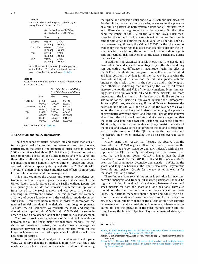
278 W. Mensi et al. / Journal of Banking and Finance 75 (2017) 258–279
Table 10
Results of short- and long-run �CoVaR asym-
metry from oil to stock markets.
H 0 : �CoVa R Short = �CoVa R Long
H 1 : �CoVa R Short � = �CoVa R Long
Down Up
S&P500 0.1879 0.1870
[0.0 0 0 0] [0.0 0 0 0]
Stoxx600 0.8094 0.8048
[0.0 0 0 0] [0.0 0 0 0]
TSX 0.7154 0.7002
[0.0 0 0 0] [0.0 0 0 0]
DJPI 0.8939 0.8957
[0.0 0 0 0] [0.0 0 0 0]
Note: The values in brackets [ ] are the p-values
of the K–S test. The delta conditional value-at-
risk ( �CoVaR) is calculated using Eq. (22) .
Table 11
Results of the down and upside �CoVaR asymmetry from
oil to stock markets.
H 0 : �CoVa R Down = �CoVa R U p
H 1 : �CoVa R Down � = �CoVa R U p
Raw Short Long
S&P500 0.7314 0.0507 0.0402
[0.0 0 0 0] [0.0 0 0 0] [0.0013]
Stoxx600 0.8608 0.0892 0.3378
[0.0 0 0 0] [0.0 0 0 0] [0.0 0 0 0]
TSX 0.9889 0.0554 0.5637
[0.0 0 0 0] [0.0 0 0 0] [0.0 0 0 0]
DJPI 0.6100 0.0322 0.1187
[0.0 0 0 0] [0.0182] [0.0 0 0 0]
Note: See the notes of Table 10.
t
f
o
l
h
s
c
h
w
s
c
t
d
r
t
a
d
i
t
i
i
i
a
S
d
a
o
e
t
A
t
k
t
m
d
s
c
s
r
o
s
d
t
p
c
s
s
f
s
e
m
q
r
m
R
A
7. Conclusion and policy implications
The dependence structure between oil and stock markets at-
tracts a great deal of attention from researchers and practitioners,
particularly in the wake of the dramatic oil price surge in summer
2008 (when it reached about $US 145 /barrel). However, oil prices
have important effects on the stock markets and vice versa but
these effects differ during bear and bull markets and under differ-
ent investment time horizons, having different upside and down-
side risk spillovers, especially during and after the 20 08–20 09 GFC.
Therefore, understanding these multifaceted effects is important
for portfolio allocation and risk management.
This study examines the average and extreme dependence be-
tween oil and four major regional developed stock markets (the
United States, Canada, Europe and the Pacific without Japan). We
also quantify the upside and downside systemic risk spillovers
from the oil to the stock markets and vice versa in the short-
and long-run investment horizons. For this purpose, we combine
a battery of copula functions with the variational mode decompo-
sition (VMD) multiresolution method in order to decompose the
marginal model’s residuals into their short and long components.
To assess the risk spillovers, we calculate the short- and long-run
downside and upside VaRs, CoVaRs and �CoVaRs risk measures in
order to have a new deeper look at the portfolio risk management.
The results provide strong evidence of dynamic tail dependence
between the oil and those major regional stock markets. For the
short-time investment horizon, the results show an average de-
pendence between the oil and the stock markets, while for the
long-run horizons we find tail dependence for all the stock mar-
kets with oil returns.
Based on the graphical analysis of the downside and upside
VaRs, we observe that the oil market is more risky than the stock
markets in both bearish and bullish market conditions. Comparing
he upside and downside VaRs and CoVaRs systemic risk measures
or the oil and stock raw return series, we observe the presence
f a similar pattern of both systemic risks for all markets, with
ow differences in magnitude across the markets. On the other
and, the impact of the GFC on the VaRs and CoVaRs risk mea-
ures for the oil and stock markets is evident as we find signifi-
ant abrupt variations during the 20 08–20 09 crisis period. The GFC
as increased significantly the VaR and CoVaR for the oil market as
ell as for the major regional stock markets, particular for the U.S.
tock market. In addition, the oil and stock markets show signifi-
ant bidirectional risk spillovers in all the cases, particularly during
he onset of the GFC.
In addition, the graphical analysis shows that the upside and
ownside CoVaRs display the same trajectory in the short and long
un, but with a low difference in magnitude. Again, the effect of
he GFC on the short- and long-run risk spillovers for the short
nd long positions is evident for all the markets. By analyzing the
ownside and upside risk, we find that oil has a greater systemic
mpact on the stock markets in the short-run and in the long-run
han otherwise, indicating that increasing the VaR of oil would
ncrease the conditional VaR of the stock markets. More interest-
ngly, both risk spillovers (to oil and to stock markets) are more
mportant in the long run than in the short-run. Similar results are
lso found for the upside risk spillovers. By using the Kolmogorov–
mirnov (K-S) test, we show significant differences between the
ownside and upside VaRs and CoVaRs for the raw series as well
s for the short- and long-run horizons, underlying the presence
f asymmetric downside short- and long-run –upside risk spillover
ffects from the oil to stock markets and vice versa, suggesting that
he short- and long-run down and upside spillovers are different.
dditionally, we find strong evidence of asymmetric behavior of
he upside and downside risk spillovers to the oil and to stock mar-
ets, with the exception of the DJPI index for the raw series and
he S&P500 index when analyzing the oil risk spillovers to stock
arkets.
Finally, using the �CoVaR risk measure we observe that the
ownside the �CoVaR is greater than the upside �CoVaR for the
tock markets (S&P500, stoxx600 and TSX indexes), with the ex-
eption of the DJPI index. By considering the time horizons, we
how that the long run down �CoVaR is higher than the short
un down �CoVaR for the S&P500, TSX and DJIP indexes. More-
ver, we find asymmetric downside and upside �CoVaRs at the
hort- and long-run horizons. The results also reveal asymmetric
ownside and upside �CoVaRs for the raw series as well as for
he short- and long horizons.
These findings have several important implication for investors,
ortfolio managers and traders. All market participants should be
ognizant of the bidirectional risk spillovers between the oil and
tock markets for both the short and long positions. They also
hould consider the time horizons when they manage their port-
olios. The portfolio managers should hedge and adjust their po-
itions in consideration of investment horizons. As for policymak-
rs, they should remain vigilant of the effects of oil price extreme
ovements on the stock markets and intervene, whenever is re-
uired, to keep the operation of the stock markets stable and less
isky, having the broader objective of systemic financial stability in
ind.
eferences
badie, A. , 2002. Bootstrap tests for distributional treatment effects in instrumental
variables models. J. Am. Stat. Assoc. 97, 284–292 .
Adrian, T., Brunnermeier, M.K., 2011. CoVaR. Working paper, Federal Reserve Bank ofNew York.
Arouri, M.E.H. , Nguyen, D.K. , 2010. Oil prices, stock markets and portfolio invest-ment: evidence from sector analysis in europe over the last decade. Energy Pol-
icy 38, 4528–4539 .

W. Mensi et al. / Journal of Banking and Finance 75 (2017) 258–279 279
A
B
B
B
B
C
C
C
C
D
D
D
D
E
FG
H
H
H
J
J
J
K
K
K
L
L
L
M
M
NP
P
R
R
S
S
S
V
W
Y
loui, R. , Hammoudeh, S. , Nguyen, D.K. , 2013. A time-varying copula approach to oiland stock market dependence: the case of transition economies. Energy Econ.
39, 208–221 . aillie, R.T. , Bollerslev, T. , Mikkelsen, H.O. , 1996. Fractionally integrated generalized
auto-regressive conditional heteroskedasticity. J. Econ. 74, 3–30 . alcilar, M. , Gupta, R. , Miller, S-M. , 2015. Regime switching model of US crude oil
and stock market prices: 1859 to 2013. Energy Econ. 49, 317–327 . alcilar, M. , Ozdemir, Z.A. , 2013. The causal nexus between oil prices and equity
market in the U.S.: a regime switching model. Energy Econ. 39, 271–282 .
jørnland, H.C. , 2009. Oil price shocks and stock market booms in an oil exportingcountry. Scott. J. Polit. Econ. 56, 232–254 .
herubini, U. , Luciano, E. , Vecchiato, W. , 2004. Copula methods in finance. Chich-ester, UK, John Willey & Sons .
hen, N.F. , Roll, R. , Ross, S. , 1986. Economic forces and the stock market. J. Bus. 59,383–403 .
iner, C. , 2001. Energy shocks and financial markets: nonlinear linkages. Stud. Non-
linear Dyn. Econ. 5, 1–11 . ong, R.G. , Wei, Y.M. , Jiao, J.-L. , Fan, Y. , 2008. Relationships between oil price
shocks and stock market: an empirical analysis from china. Energy Policy 36(9), 3544–3553 .
ickey, D. , Fuller, W. , 1979. Distribution of the estimators for autoregressive timeseries with a unit root. J. Am. Stat. Assoc. 74, 427–431 .
ing, H. , Kimb, H-G. , Park, S-Y. , 2016. Crude oil and stock markets: causal relation-
ships in tails? Energy Econ. 59, 58–69 . ragomiretskiy, K. , Zosso, D. , 2014. Variational mode decomposition. IEEE Trans. Sig-
nal Process 62, 531–544 . u, L. , He, Y. , 2015. Extreme risk spillovers between crude oil and stock markets.
Energy Econ. 51, 455–465 . ngle, R.F. , 1982. Autoregressive conditional heteroskedasticity with estimates of the
variance of United Kingdom inflation. Econometrica 50, 987–1007 .
isher, I. , 1930. The Theory of Interest. New York, p. 43 . irardi, G. , Ergün, A.T. , 2013. Systemic risk measurement: multivariate GARCH esti-
mation of covar. J. Bank. Financ. 37, 3169–3180 . ansen, B.E. , 1994. Autoregressive conditional density estimation. Int. Econ. Rev. 35,
705–730 . osking, J.R.M. , 1980. The multivariate portmanteau statistic. J. Am. Stat. Assoc. 75,
602–608 .
uang, D.R. , Masulis, R.W. , Stoll, H. , 1996. Energy shocks and financial markets. J.Futures Mark. 16, 1–27 .
iménez-Rodríguez, R. , Sánchez, M. , 2005. Oil price shocks and real GDP growth:empirical evidence for some OECD countries. Appl. Econ. 37, 201–228 .
oe, H. , 1997. Multivariate models and dependence concepts. Monographs in Statis-tics and Probability 73. London, Chapman and Hall .
ones, C.M. , Kaul, G. , 1996. Oil and the stock markets. J. Financ. 51, 463–491 .
ang, W. , Ratti, R.A. , Yoon, K.Y. , 2015. Time-varying effect of oil market shocks onthe stock market. J. Bank Financ. 61, S150–S163 .
ling, J. , 1985. Oil price shocks and stock-market behavior. J. Portfolio Manag. 12,34–39 .
wiatkowski, D. , Phillips, P.C.B. , Schmidt, P. , Shim, Y. , 1992. Testing the null hypoth-esis of stationarity against the alternative of a unit root: how sure are we that
economic time series are non-stationary? J. Econ. 54, 159–178 . i, Z. , Chen, J. , Zi, Y. , Pan, J. , 2017. Independence-oriented VMD to identify fault fea-
ture for wheel set bearing fault diagnosis of high speed locomotive. Mech. Syst.Signal Process. 85, 512–529 .
iu, X. , An, H. , Huang, S. , Wen, S. , 2016. The evolution of spillover effects between
oil and stock markets across multi-scales using a wavelet-based GARCH-BEKKmodel. Physica A: Stat. Mech. Appl. 65, 374–383 .
u, F., Qiao, H., Wang, S., Lai, K.K., Li, Z., 2016. Time-varying coefficient vector autore-gressions model based on dynamic correlation with an application to crude oil
and stock markets. Environ. Res. forthcoming, http://dx.doi.org/10.1016/j.envres.2016.07.015 .
cLeod, A.I. , Li, W.K. , 1983. Diagnostic checking ARMA time series models using
squared residual autocorrelations. J. Time Ser. Anal. 4, 269–273 . ohanty, S. , Nandha, M. , Bota, G. , 2010. Oil shocks and stock returns: the case of the
central and Eastern European (CEE) oil and gas sectors. Emerg. Markets Review11, 358–372 .
elsen, R.B. , 2006. An Introduction to Copulas. New York, Springer-Verlag . atton, A.J. , 2006. Modelling asymmetric exchange rate dependence. Int. Econ. Rev.
47, 527–556 .
hilips, P.C.B. , Perron, P. , 1988. Testing for unit roots in time series regression.Biometrika 75, 335–346 .
aza, N. , Shahzad, S.H. , Tiwari, A.K. , Shahbaz, M. , 2016. Asymmetric impact of gold,oil prices and their volatilities on stock prices of emerging markets. Resour. Pol-
icy 49, 290–301 . eboredo, J.C. , Ugolini, A. , 2015. Systemic risk in European sovereign debt markets:
A CoVaR-copula approach. J. Int. Money Fin. 51, 214–244 .
adorsky, P. , 1999. Oil price shocks and stock market activity. Energy Econ. 21,449–469 .
adorsky, P. , 2012. Correlations and volatility spillovers between oil prices andthe stock prices of clean energy and technology companies. Energy Econ. 34,
248–255 . im, N. , Zhou, H. , 2015. Oil prices, US stock return, and the dependence between
their quantiles. J. Bank Financ. 55, 1–8 .
o, M. , 2011. Oil and stock market volatility: a multivariate stochastic volatility per-spective. Energy Econ. 33, 956–965 .
illiams, J.B. , 1938. The Theory of Investment Value. Harvard University Press, Cam-bridge, Mass. .
ang, L. , Zhu, Y. , Wang, Y. , Wan, Y. , 2016. Multifractal detrended cross-correlationsbetween crude oil market and Chinese ten sector stock markets. Physica A: Stat.
Mech. Appl. 462, 255–265 .