Journal of Atmospheric and Solar-Terrestrial Physics 73 (2011) 323–334

Contents lists available at ScienceDirect

Journal of Atmospheric and Solar-Terrestrial Physics

1364-68

doi:10.1

� Corr

E-m

journal homepage: www.elsevier.com/locate/jastp

USGS 1-min Dst index

J.L. Gannon �, J.J. Love

USGS Geomagnetism Program, Denver, CO, USA

a r t i c l e i n f o

Article history:

Accepted 8 February 2010We produce a 1-min time resolution storm-time disturbance index, the USGS Dst, called Dst .

This index is based on minute resolution horizontal magnetic field intensity from low-latitude

Available online 15 February 2010

Keywords:

Magnetosphere

Ring current

Dst

Disturbance index

26/$ - see front matter Published by Elsevier

016/j.jastp.2010.02.013

esponding author. Tel.: +1 303 273 8487.

ail address: jgannon@usgs.gov (J.L. Gannon).

a b s t r a c t

8507-4SM

observatories in Honolulu, Kakioka, San Juan and Hermanus, for the years 1985–2007. The method used

to produce the index uses a combination of time- and frequency-domain techniques, which more

clearly identifies and excises solar-quiet variation from the horizontal intensity time series of an

individual station than the strictly time-domain method used in the Kyoto Dst index. The USGS 1-min

Dst is compared against the Kyoto Dst, Kyoto Sym-H, and the USGS 1-h Dst (Dst5807-4SH). In a time series

comparison, Sym-H is found to produce more extreme values during both sudden impulses and main

phase maximum deviation, possibly due to the latitude of its contributing observatories. Both Kyoto

indices are shown to have a peak in their distributions below zero, while the USGS indices have a peak

near zero. The USGS 1-min Dst is shown to have the higher time resolution benefits of Sym-H, while

using the more typical low-latitude observatories of Kyoto Dst.

Published by Elsevier Ltd.

1. Introduction

Ground-based magnetic field observations have a componentthat is reflective of the Earth’s space environment and provideimportant information about the state of geomagnetic activity.The competing balance between Earth’s intrinsic magnetic fieldand solar wind dynamic pressure drives much of the variation ofthe Earth’s space environment (see, e.g. Russell, 2000). Forexample, sudden increases in solar wind density or velocitycompress the day-side magnetopause, which result in enhance-ments and rearrangements of the complex current systems nearthe Earth. These current system changes are observed as magneticfield fluctuations at ground-level (McPherron, 1995).

The World Data Center in Kyoto uses ground-based magneticfield measurements to produce a global disturbance index calledDst, developed by Sugiura (1964). The Kyoto Dst index is used tocharacterize deviations from the quiet-time horizontal magneticfield during times of geomagnetic disturbance. It is produced witha 1-h time resolution and is continuous in time back to 1957. Theindex has been modified and improved over the years (e.g.Sugiura and Hendricks, 1967; Sugiura and Kamei, 1991; Karinenand Musula, 2006), but the essentially time-domain nature of themethod has remained unchanged for over 50 years.

The Dst index is commonly used as an indicator of geomag-netic activity, including identification of storms, which have acritical influence on particle populations, satellites and other

Ltd.

human activity in space (e.g. Reeves et al., 2003). These stormshave a classical multi-phase form observed in ground-basedmagnetic field measurements (Chapman, 1919), each having adistinctive shape and time scale: sudden commencement, initialphase, main phase and recovery phase. The sudden commence-ment occurs as the initial impact of increased solar wind dynamicpressure sharply compresses the magnetopause. At the ground,this is observed as a sharp increase in horizontal magnetic fieldintensity on time scales of less than 1 h. The main phase andrecovery phases are characterized by a decrease in horizontalmagnetic field intensity and then slow return to baseline. Thestrength of a geomagnetic storm is described by the minimumreached during the main phase (Gonzalez et al., 1994).

The 1-h time resolution of the Kyoto Dst is insufficient whenresearchers need to study effects that occur on sub-hour timescales, such as storm sudden commencements. The Kyoto Sym-Hindex is a 1-min time resolution index produced using a similarmethod as the Kyoto Dst (Iyemori, 1990). It provides higher timeresolution than the Kyoto Dst, but Sym-H is inherently differentbecause of the mid-latitude location of the observatories that areused. Because magnetic disturbance varies with latitude (Arakiet al., 1997) and proximity to regional current systems con-tributes to the intensity of an observed magnetic signal, the Sym-H index can reflect different physical processes than a low-latitude index, especially during times of geomagnetic activity.

In this paper we apply the time and frequency space method ofLove and Gannon (2009) to minute resolution horizontalmagnetic deviation data from low-latitude magnetometerstations to produce a low-latitude Dst index with a 1-min timeresolution. In the frequency domain, the observatory data display

J.L. Gannon, J.J. Love / Journal of Atmospheric and Solar-Terrestrial Physics 73 (2011) 323–334324

a prominent set of stationary Fourier harmonics having periodsequal to integer fractions of the Earth’s rotational period, theMoon’s orbital period, the Earth’s orbital period, and the cross-coupling of harmonics with those periods. These harmonicsdominate what is commonly described as solar-quiet variation,and are clearly identifiable in the frequency domain.Non-stationary contributions to the magnetic field timeseries, such as the secular variation of the Earth’s magneticfield, are necessarily treated in the time domain. This indexprovides a measure of low-latitude disturbance with solar-quietvariation cleanly removed, and is produced with a sufficientresolution for analysis of physical processes with time scales lessthan an hour.

2. Data

Magnetic observatories are specially designed and carefullyoperated facilities that provide accurate data over long periods oftime (e.g. Love, 2008). The data are collected using a digitalacquisition system, and is combined with additional calibrationdata to produce time series that have long-term stability andaccuracy, usually much better than 5 nT.

The Kyoto Dst index is calculated using hour resolutionhorizontal magnetic field intensity from four standard observatorieschosen for their even longitudinal-spacing (Mendes et al., 2006),data quality, and continuity. Low-latitude (but not equatorial)positioning is also desired to avoid the signal from being dominatedby the equatorial electrojet or auroral current systems. Theobservatories are Hermanus (HER) South Africa, Kakioka (KAK)Japan, Honolulu (HON) Hawaii, and San Juan (SJG) Puerto Rico.

In this analysis, we use the minute resolution horizontalmagnetic intensity data to produce a 1-min resolution Dst index,calculated for the period 1985–2007. For simplicity and consis-tency with the Kyoto Dst, we use these same standard stations,although, in principle, we are not limited to these four. The23 year reanalysis time span is chosen due to data availability ofthe minute resolution data, which extends back at least to 1985for these observatories.

The percentage of missing data in each of the observatory timeseries is small (or literally zero for KAK). Operational changesresulting in abrupt offsets are usually well documented or easilyidentified upon inspection of the time series. The World DataCenters in Edinburgh and Kyoto and the Intermagnet consortium

Fig. 1. Honolulu horizontal intensity (1985–2007). O

provide definitive data which has been processed to remove baselineoffsets and data spikes, at 1.0 and 0.1 nT precision, respectively. Thetime stamps are assigned at the top of the minute. Sym-H isobtained from the World Data Center in Kyoto, and uses data fromvarying combinations of mid-latitude stations.

3. Method

In this calculation we use the method detailed in Love andGannon (2009), which combines time and frequency spaceanalyses to isolate the disturbance signal from a magnetic fieldtime series measured at a given observatory. Fig. 1 shows the datafrom the HON observatory, for the entire analysis time period of1985–2007. There are multiple, overlapping magnetic fieldcontributions that are reflected in the individual periodicitiesevident in the time series, as well as a long-term drift in intensity.The magnetic field horizontal component time series (H) is asuperposition of contributions from the Earth’s internal field andexternal current systems. The internal components mainlycomprised slowly varying magnetic variations arising from thedynamo in the Earth’s core (e.g. Jackson and Finlay, 2007) and alsoinclude contributions from the crust (e.g. Purucker and Whaler,2007). For the purpose of this analysis, we label all long term,slowly varying drifts as secular variation (SV). The externalcomponents, including the non-periodic disturbance (Dist) signal,are composed of periodic contributions by ionospheric currentsystems (e.g. Campbell, 1989) and variations due to knownperiodic influences from the magnetosphere (SQ) and solar cycle(SC) (e.g. Clua de Gonzalez et al., 1993). In order to isolate Dist, wemust first identify and remove the other contributing signals:

H¼ SVþSqþSCþDist: ð1Þ

The computational methodology outlined in Fig. 2 represents asummary of the process adapted to the minute time resolutiondata. We begin with the horizontal component magnetic fieldtime series for an individual observatory. In each step, we removeone of the following components: secular (SV), solar cycle (SC)and solar-quiet (SQ) variation.

3.1. Internal contributions to magnetic signal–secular variation

We first identify and remove the most slowly varyingcomponents of the magnetic field time series—the secular

verlaid is the estimated secular variation curve.

J.L. Gannon, J.J. Love / Journal of Atmospheric and Solar-Terrestrial Physics 73 (2011) 323–334 325

variation of the geomagnetic main field arising from convectivefluid motion in the Earth’s core. This is seen in the observatorydata as a slow drift in the magnetic vector over periods of decades.

Fig. 2. Flowchart of USGS Ds

Fig. 3. Time series showing data with secular variation subtracted. Overlaid in green

analysis. (b) shows a close-up for the time period February 23–March 25, 2001, as an ex

is referred to the web version of this article.)

Because no periodicities are resolved over the time span of thisanalysis, the identification of SV is done in the time domain. SV isnot dependent on or affected by external current systems, and so

t calculation algorithm.

is the storm-interpolated time series. (a) shows the entire time span used in this

ample. (For interpretation of the references to color in this figure legend, the reader

J.L. Gannon, J.J. Love / Journal of Atmospheric and Solar-Terrestrial Physics 73 (2011) 323–334326

it is best identified during the quietest times of the time series,during which there should be the smallest contribution fromexternal current systems. We use the following algorithm toselect quiet days, using a 24-h sliding window, within which wemeasure the average of absolute hour-to-hour differences:

dHi ¼1

24

X24

m ¼ 1

JHiþm�Hiþm�1J; ð2Þ

where the quantity is not calculated if more than half of the dataare missing. For each month, the five smallest dHi valuesdetermine the five quietest days, which we note do notnecessarily correspond to whole universal-time days, nor do theynecessarily correspond exactly to International Quiet Days,although there is often significant overlap. A truncated Chebyshevpolynomial (Press et al., 2007) is fit to a time series of dailyaverages of the selected quiet-time periods and is subtracted fromthe observatory time series, effectively zero baseline detrendingthe data. In Fig. 1, the curve overlaying the observatory datashows the calculated SV polynomial for the HON time series. Afterthe subtraction of SV, the time series contains only componentsdue to external current systems and their inductive effects on theEarth (see Fig. 3).

H�SV ¼ SqþSCþDist: ð3Þ

Fig. 4. Time series showing the solar-quiet variation, which is selected in the frequency

for the time period February 23–March 25, 2001, as an example.

3.2. Solar-quiet variation

We identify solar-quiet variation as the periodic signalsidentified in the power spectrum seen in Fig. 4. These peaks inthe spectrum are of relatively higher power than the surroundingfrequencies, and can be identified as stationary Fourier harmonicshaving periods equal to integer fractions of the Earth’s rotationalperiod, the Moon’s orbital period, the Earth’s orbital period, andthe cross-coupling of harmonics with those periods. We use acombination of time and frequency space techniques to isolate SQand produce a time series which will be subtracted as the nextstep in the formulation of our Dst index.

We first do a rough cut of the disturbance signal in the timedomain by selecting particularly disturbed time periods andinterpolating across days during these times. This is done for eachindividual observatory time series by first ranking the hourlyvalues of the H�SV time series. Starting with the largest value, weopen up a window of time that begins (ends) at least 12 h before(after)—the duration of the time window is at least 25 h in length,and its actual duration determined by a simple threshold criterionfor maximum value within a sliding 12-h span of time. Thisenables us to define an active duration that commences before(ends after) the maximum point. We then remove all points fromthis identified active duration and substitute value interpolatedbetween data corresponding to the same time-of-day according to

domain. (a) shows the entire data span used in this analysis. (b) shows a close-up

J.L. Gannon, J.J. Love / Journal of Atmospheric and Solar-Terrestrial Physics 73 (2011) 323–334 327

the formula:

Ei ¼1

mþnðnEi�24mþmEiþ24nÞ; ð4Þ

where i denotes an instance in time, and m (n) is the number ofdays without missing data preceding (following) the day withmissing data. The remaining values are then ranked again, and theprocess of disturbance identification and interpolation is repeateduntil a termination threshold is reached. Fig. 3(b) shows anexample of this storm time interpolation. Note from Fig. 3(b) thatboth the storm-interpolated time series and the external signalhave an obvious diurnal variation.

The storm-interpolated time series is then transformed to thefrequency domain using a fast Fourier transform (FFT) (Press et al.,2007). The spectral peaks of components with periodicities thatwe consider to be solar-quiet variation are highlighted in Fig. 5(a).The peaks are well defined and are split due to modulation byother periodic influences. For example, the daily peak is evident at1 day, and is flanked by a set of smaller peaks, due to spectral linebroadening from modulation of the diurnal variation by solarcycle, the influence of the moon, and solar rotation. The Sq

variation can be represented by a three-dimensional Fourierseries of the form:

SqðtÞ ¼RXid;m;a

sqid;m;aeiðidodþ imomþ iaoaÞt

( ): ð5Þ

We band pass the Sq coefficients that correspond to narrowwindows centered on each of these peaks in the frequencydomain and reverse transform the selected components to thetime domain using a reverse FFT to produce an SQ time seriescomposed entirely of a signal of our selected frequencies, applying

Fig. 5. Frequency-domain depiction of raw data and storm-interpolated data, with sol

shows a close-up of the one day period. (For interpretation of the references to color i

the filtering to a finite number of harmonic terms. We adjust thewidth of the passing windows for each harmonic term so that,roughly speaking, the widest windows correspond to thosefrequencies having the greatest power.

We subtract the SQ time series (Fig. 4) from the external signalshown in Fig. 3 to yield a time series that contains the remainingSC and Dist signals.

H�SV�Sq¼ SCþDist: ð6Þ

3.3. Solar cycle variation

We now identify, in the frequency domain, longer time periodvariations remaining in the time series from the solar cycle. This isa semi-periodic signal, but because of the variable length of thesolar cycle, it will appear as a band of frequencies which are notwell resolved using the data set available for minute resolutionanalysis. To remove long period variations, we transform again(this time using a time series where the highly disturbed periodsare not removed) to frequency space and use a lowpass filter toremove all frequencies greater than 10 years. The components ofSC are highlighted in Fig. 5 in the frequency domain.

The remaining components are transformed back to the timedomain with all long period contributions removed (see Fig. 4).Although we do this in the frequency domain, it is equivalent toidentifying SC frequencies, transforming the selection back to thetime domain and subtracting it from the initial signal (Fig. 4shows the SC curve in the time domain). This leaves us with thedisturbance signal, Dist, for an individual observatory time series.

H�SV�Sq�SC ¼Dist: ð7Þ

ar-quiet frequencies highlighted in blue. (a) shows the entire frequency space. (b)

n this figure legend, the reader is referred to the web version of this article.)

Fig. 6. Time series showing the data series with secular variation, solar-quiet variation and solar cycle variation subtracted. (a) shows the entire data span used in this

analysis. (b) shows a close-up for the time period February 23–March 25, 2001, for the four standard observatories used in this analysis. Separation factors have been applied.

J.L. Gannon, J.J. Love / Journal of Atmospheric and Solar-Terrestrial Physics 73 (2011) 323–334328

3.4. Disturbance signal

The remaining, isolated Dist signal is the deviation inhorizontal magnetic field due to non-stationary changes instorm-time current systems. Fig. 6 shows the disturbance timeseries for HON, with Fig. 6(b) additionally showing the SJG, HERand KAK signals. Looking at Fig. 6(b), the diurnal signal that wasobvious in Fig. 3 is now distinctly diminished. The differencesbetween the Dist curves from different observatories are due tolongitudinal variations in storm-time disturbance signal.

3.5. USGS 1-min Dst

The disturbance signals for individual observatories are nowcombined to produce our Dst index. Each time series stationis weighted by 1=coslB, where lB is the observatory site’smagnetic latitude. The weighted time series are then averagedto produce the minute resolution Dst index, shown in Fig. 7. Wewill refer to this index, using this span of time (1985–2007)and this subset of stations (the four standard at the minuteresolution, or 4SM), as Dst8507-4SM. The time series in Fig. 7(a)and (b) look very similar to the individual magnetometerdisturbance traces, with the four storms smoothly deviatingfrom the quiet intervening periods, which contain no stationaryperiodic variation.

4. Analysis

4.1. Time series comparison

In order to understand the contributions of method and inputto Dst8507-4SM, we compare the time series to that of Sym-H,Dst5807-4SH, and the Kyoto Dst (see Table 1 for a summary of theproperties of each index). Sym-H has a 1-min time resolution likeDst8507-4SM and is used often when a higher resolution index isrequired for scientific analysis. It is produced by the World DataCenter in Kyoto, Japan, following the essentially time-domainmethod of the hourly Kyoto Dst index, but using 1-min timeresolution input from a set of mid-latitude observatories. Becauseof the known variation of geomagnetic disturbance propagationwith magnetic latitude, we would expect the use of data frommid-latitude observatories to affect the final disturbance signal.Previous work by Wanliss and Showalter (2006) has shown thatKyoto Dst and Sym-H have reasonable correlation, divergingsomewhat for values lower than �300 nT, and suggests that thebenefits of the improved 1-min time resolution of Sym-H versusthe 1-h Kyoto Dst outweighs any problems observed in Sym-H.

Fig. 10 shows an example time period, including theHalloween storm of 2003, for each combination of two indices.The overlaid green curve is the point-by-point difference betweeneach pair of indices, where averaging is used when a timeresolution difference exists. The main differences can be seen

Fig. 7. Time series showing the calculated 1-min USGS Dst. (a) shows the entire data span used in this analysis. (b) shows a close-up for the time period February 23–March

25, 2001, as an example.

Table 1Summary of index formulation.

Index Method Resolution Input

Dst8507-4SM Time/frequency

domain

1-min Four standard

low-latitude

Dst5807-4SH Time/frequency

domain

1-h Four standard

low-latitude

Kyoto Dst Time domain 1-h Four standard

low-latitude

Kyoto Sym-H Time domain 1-min Various mid-latitude

J.L. Gannon, J.J. Love / Journal of Atmospheric and Solar-Terrestrial Physics 73 (2011) 323–334 329

during storm main phase. The smallest storm-time differencesappear between the two USGS indices. The largest storm-timedifferences occur between Sym-H and any other index. Sym-Halso shows greater variability during the relatively quiet timessurround the storm, when compared to the three other indices. Tounderstand the general relative behavior of longer time series, weplot each index against each other. Fig. 11 shows correlation plotsfor the period 1985–2003 (the subset of time when the KyotoFinal Dst results are available), for pairs of indices. The overlaidline indicates perfect correlation, and in comparison we canquickly see how far each index deviates from the otherwith activity level. Sym-H and Kyoto Dst are highly correlated,and the two USGS indices (1-min and 1-h time resolution) are alsohighly correlated. In contrast, when comparing Sym-H and

Dst8507-4SM, we see that Sym-H produces generally moreextreme values than the USGS index during disturbed times. Inthe case of Sym-H versus Dst8507-4SM, the hourly averaged indicesare overlaid to facilitate a comparison to the other panels, where60 times fewer points are available. There are some differencesbetween Sym-H and Dst8507-4SM during times of higher activitythat are particularly obvious using the un-averaged indices. Thefarthest outlying points correspond to the 2003 Halloween Storm.These deviations are less obvious on the hourly averagedcomparison of the same two indices suggesting that the widevariation of Sym-H in comparison to hourly storm indices mayhave been previously understated, particularly during storm-time(Fig. 12).

Over the 23 reanalysis period, on average, Sym-H is7.6 nT lower than Dst4SH-8507. Fig. 13 shows the probabilitydistributions of each index, further illustrating the differences.The shape of each distribution is similar, however indices ofsimilar method (USGS 1-min/1-h and Kyoto Dst/Sym-H) havedifferent peak distribution points. The USGS indices have amaximum likelihood of near 0, while for the Kyoto indices it isbelow zero.

4.2. Storm-time comparison

The previous sections described an overview of the availableindices and a general comparison of the time series. In order to

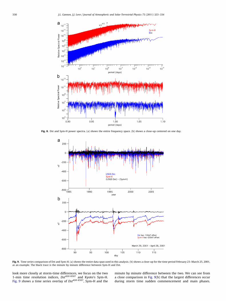
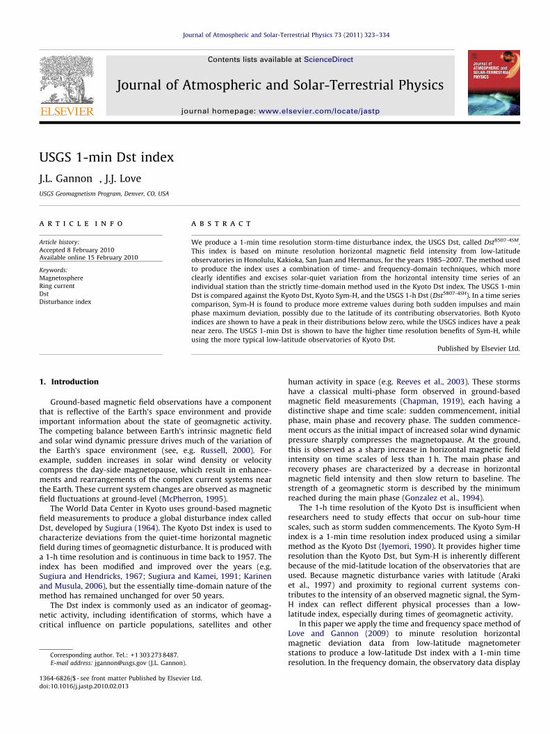
Fig. 8. Dst and Sym-H power spectra. (a) shows the entire frequency space. (b) shows a close-up centered on one day.

Fig. 9. Time series comparison of Dst and Sym-H. (a) shows the entire data span used in this analysis. (b) shows a close-up for the time period February 23–March 25, 2001,

as an example. The black trace is the minute by minute difference between Sym-H and Dst.

J.L. Gannon, J.J. Love / Journal of Atmospheric and Solar-Terrestrial Physics 73 (2011) 323–334330

look more closely at storm-time differences, we focus on the two1-min time resolution indices, Dst4SH-8507 and Kyoto’s Sym-H.Fig. 9 shows a time series overlay of Dst4SH-8507, Sym-H and the

minute by minute difference between the two. We can see froma close comparison in Fig. 9(b) that the largest differences occurduring storm time sudden commencement and main phases.

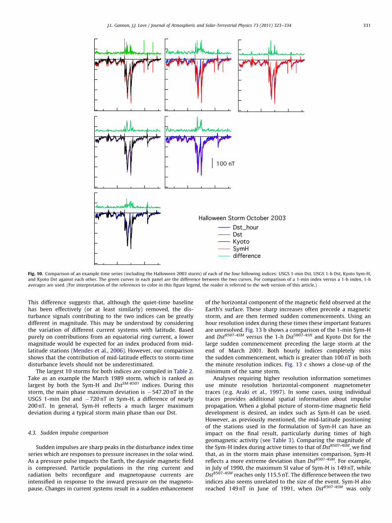
Fig. 10. Comparison of an example time series (including the Halloween 2003 storm) of each of the four following indices: USGS 1-min Dst, USGS 1-h Dst, Kyoto Sym-H,

and Kyoto Dst against each other. The green curves in each panel are the difference between the two curves. For comparison of a 1-min index versus a 1-h index, 1-h

averages are used. (For interpretation of the references to color in this figure legend, the reader is referred to the web version of this article.)

J.L. Gannon, J.J. Love / Journal of Atmospheric and Solar-Terrestrial Physics 73 (2011) 323–334 331

This difference suggests that, although the quiet-time baselinehas been effectively (or at least similarly) removed, the dis-turbance signals contributing to the two indices can be greatlydifferent in magnitude. This may be understood by consideringthe variation of different current systems with latitude. Basedpurely on contributions from an equatorial ring current, a lowermagnitude would be expected for an index produced from mid-latitude stations (Mendes et al., 2006). However, our comparisonshows that the contribution of mid-latitude effects to storm-timedisturbance levels should not be underestimated.

The largest 10 storms for both indices are compiled in Table 2.Take as an example the March 1989 storm, which is ranked aslargest by both the Sym-H and DstSM-8507 indices. During thisstorm, the main phase maximum deviation is �547.20 nT in theUSGS 1-min Dst and �720 nT in Sym-H, a difference of nearly200 nT. In general, Sym-H reflects a much larger maximumdeviation during a typical storm main phase than our Dst.

4.3. Sudden impulse comparison

Sudden impulses are sharp peaks in the disturbance index timeseries which are responses to pressure increases in the solar wind.As a pressure pulse impacts the Earth, the dayside magnetic fieldis compressed. Particle populations in the ring current andradiation belts reconfigure and magnetopause currents areintensified in response to the inward pressure on the magneto-pause. Changes in current systems result in a sudden enhancement

of the horizontal component of the magnetic field observed at theEarth’s surface. These sharp increases often precede a magneticstorm, and are then termed sudden commencements. Using anhour resolution index during these times these important featuresare unresolved. Fig. 13 b shows a comparison of the 1-min Sym-Hand Dst8507-4SM versus the 1-h Dst5807-4SH and Kyoto Dst for thelarge sudden commencement preceding the large storm at theend of March 2001. Both hourly indices completely missthe sudden commencement, which is greater than 100 nT in boththe minute resolution indices. Fig. 13 c shows a close-up of theminimum of the same storm.

Analyses requiring higher resolution information sometimesuse minute resolution horizontal-component magnetometertraces (e.g. Araki et al., 1997). In some cases, using individualtraces provides additional spatial information about impulsepropagation. When a global picture of storm-time magnetic fielddevelopment is desired, an index such as Sym-H can be used.However, as previously mentioned, the mid-latitude positioningof the stations used in the formulation of Sym-H can have animpact on the final result, particularly during times of highgeomagnetic activity (see Table 3). Comparing the magnitude ofthe Sym-H index during active times to that of Dst8507-4SM, we findthat, as in the storm main phase intensities comparison, Sym-Hreflects a more extreme deviation than Dst8507-4SM. For example,in July of 1990, the maximum SI value of Sym-H is 149 nT, whileDst8507-4SM reaches only 115.5 nT. The difference between the twoindices also seems unrelated to the size of the event. Sym-H alsoreached 149 nT in June of 1991, when Dst8507-4SM was only

Fig. 11. Correlation plots for pairs of the four indices (USGS 1-min Dst, USGS 1-h Dst, Kyoto Sym-H, and Kyoto Dst), for the period 1985–2007. For comparison of a 1-min

index versus a 1-h index, 1-h averages are used. In the top left panel, USGS 1-min vs Kyoto Sym-H, the comparison of the 1-h averages is overlaid in black to facilitate

comparison with the other panels.

Fig. 12. The probability distributions for each of the four indices (USGS 1-min Dst, USGS 1-h Dst, Kyoto Sym-H, and Kyoto Dst).

J.L. Gannon, J.J. Love / Journal of Atmospheric and Solar-Terrestrial Physics 73 (2011) 323–334332

86.6 nT. In other words, the two indices are not linearly related toeach other. A large SI in Sym-H may correspond to a large SI inDst, or it may not. We also see that the hourly indices of USGS andKyoto are well correlated during these times (see example,Fig. 13), suggesting that the difference between Sym-H andDst8507-4SM lies not in method, but in the latitudinal differences ofthe observatories contributing to the product.

4.4. Spectrum comparison

In addition to time series comparisons of Dst4SH-8507 and theKyoto Dst, we can use the same frequency-domain techniques weexploited to precisely identify and excise Sq to compare thespectral components of each index and look for remainingspectral peaks in either index. In Fig. 8(a) the power spectra of

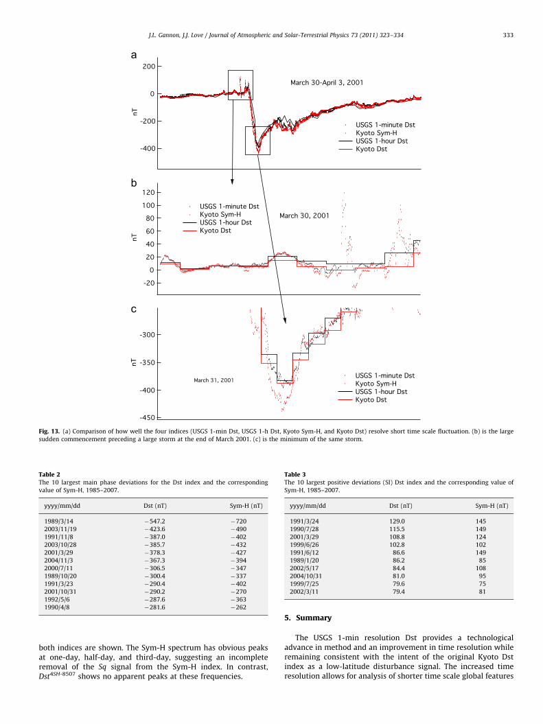
Fig. 13. (a) Comparison of how well the four indices (USGS 1-min Dst, USGS 1-h Dst, Kyoto Sym-H, and Kyoto Dst) resolve short time scale fluctuation. (b) is the large

sudden commencement preceding a large storm at the end of March 2001. (c) is the minimum of the same storm.

Table 2The 10 largest main phase deviations for the Dst index and the corresponding

value of Sym-H, 1985–2007.

yyyy/mm/dd Dst (nT) Sym-H (nT)

1989/3/14 �547.2 �720

2003/11/19 �423.6 �490

1991/11/8 �387.0 �402

2003/10/28 �385.7 �432

2001/3/29 �378.3 �427

2004/11/3 �367.3 �394

2000/7/11 �306.5 �347

1989/10/20 �300.4 �337

1991/3/23 �290.4 �402

2001/10/31 �290.2 �270

1992/5/6 �287.6 �363

1990/4/8 �281.6 �262

Table 3The 10 largest positive deviations (SI) Dst index and the corresponding value of

Sym-H, 1985–2007.

yyyy/mm/dd Dst (nT) Sym-H (nT)

1991/3/24 129.0 145

1990/7/28 115.5 149

2001/3/29 108.8 124

1999/6/26 102.8 102

1991/6/12 86.6 149

1989/1/20 86.2 85

2002/5/17 84.4 108

2004/10/31 81.0 95

1999/7/25 79.6 75

2002/3/11 79.4 81

J.L. Gannon, J.J. Love / Journal of Atmospheric and Solar-Terrestrial Physics 73 (2011) 323–334 333

both indices are shown. The Sym-H spectrum has obvious peaksat one-day, half-day, and third-day, suggesting an incompleteremoval of the Sq signal from the Sym-H index. In contrast,Dst4SH-8507 shows no apparent peaks at these frequencies.

5. Summary

The USGS 1-min resolution Dst provides a technologicaladvance in method and an improvement in time resolution whileremaining consistent with the intent of the original Kyoto Dstindex as a low-latitude disturbance signal. The increased timeresolution allows for analysis of shorter time scale global features

J.L. Gannon, J.J. Love / Journal of Atmospheric and Solar-Terrestrial Physics 73 (2011) 323–334334

such as sudden impulses and can provide an alternative to the useof Sym-H when a 1-min time resolution index is required forscientific analysis. On comparison to Sym-H, which is calculatedfrom mid-latitude stations, strong differences are apparent duringstorm time.

Acknowledgments

We thank the Japan Meteorological Agency and the SouthAfrican National Research Foundation for their commitment tothe long-term operation, respectively, of the Kakioka andHermanus magnetic observatories. We acknowledge Intermagnet(www.intermagnet.org) for its role in promoting high standards ofmagnetic-observatory practice. We thank the former World DataCenter at Copenhagen, and the present World Data Centers atKyoto and Edinburgh. We thank J.C. Green, C.A. Finn and T. Whitefor reviewing a draft manuscript. We thank two anonymousreferees for their reviews of the submitted draft manuscript. Wethank E.A. McWhirter Jr. for help with data format conversion.This work and the present operation of the Honolulu and San Juanobservatories are supported by the USGS Geomagnetism Program.

References

Araki, T., Fujitani, S., Emoto, M., Yumoto, K., Shiodawa, K., Ichinose, T., Luehr, H.,Orr, D., Milling, D.K., Singer, H., Rostoker, G., Tsunomura, S., Yamada, Y., Liu,C.F., 1997. Anomalous sudden commencement on March 24, 1991. J. Geophys.Res. 102 (A7), 14075–14086.

Campbell, W.H., 1989. The regular geomagnetic field variations during quiet solarconditions. In: Jacobs, J.A. (Ed.), Geomagnetism, vol. 3. Academic Press,London, UK, pp. 385–460.

Chapman, S., 1919. An outline of the theory of magnetic storms. Proc. R. Soc.London Ser. A 95, 61.

Cl0ua de Gonzalez, A.L., Gonzalez, W.D., Dutra, S.L.G., Tsurutani, B.T., 1993. Periodicvariation in the geomagnetic activity: a study based on the Ap index.J. Geophys. Res. 98, 9215–9231.

Gonzalez, W.D., Joselyn, J.A., Kamide, Y., Kroehl, H.W., Rostoker, G., Tsurutani, B.T.,Vasyliunas, V.M., 1994. What is a geomagnetic storm? J Geophys. Res. 99,5771.

Iyemori, T., 1990. Storm-time magnetospheric currents inferred from mid-latitudegeomagnetic field variations. J. Geomagn. Geoelectr. 42, 1249.

Jackson, A., Finlay, C.C., 2007. Geomagnetic secular variation and its applications tothe core. In: Kono, M. (Ed.), Geomagnetism, Treatise on Geophysics, vol. 5.Elsevier Science, New York, NY, pp. 147–193.

Karinen, A., Mursula, K., 2006. A new reconstruction of the Dst index for1932–2002. J. Geophys. Res. 11, A08207 , doi:10.1029/2005JA011299.

Love, J.J., 2008. Magnetic monitoring of Earth and space. Phys. Today 61, 31–37.Love, J.J., Gannon, J.L., 2009. Revised Dst and the epicycles of magnetic disturbance:

1958–2007. Ann. Geophys. 27, 3101–3131.McPherron, R.L., 1995. Magnetospheric dynamics. In: Russell, C.T., Kivelson, M.G.

(Eds.), Introduction to Space Physics. Cambridge University Press, Cambridge,UK, pp. 400–458.

Mendes, O., Mendes da Costa, A., Bertoni, F.C.P., 2006. Effects of the number ofstations and time resolution on Dst derivation. J. Atmos. Solar Terr. Phys. 68,2127–2137.

Press, W.H., Teukolsky, S.A., Vetterling, W.T., Flannery, B.P., 2007. NumericalRecipes 3rd Edition: The Art of Scientific Computing. Cambridge UniversityPress, Cambridge.

Purucker, M.E., Whaler, K.A., 2007. Crustal magnetism. In: Kono, M. (Ed.),Geomagnetism, Treatise on Geophysics, vol. 5. Elsevier Science, New York,NY, pp. 195–235.

Reeves, G.D., McAdams, K.L., Friedel, R.H.W., O’Brien, T.P., 2003. Acceleration andloss of relativistic electrons during geomagnetic storms. Geophys. Res. Lett. 30(10), 1529 , doi:10.1029/2002GL016513.

Russell, C.T., 2000. The solar wind interaction with the Earth’s magnetsphere: atutorial. IEEE Trans. Plasma Sci. 28, 1818–1830.

Sugiura, M., 1964. Hourly values of equatorial Dst for the IGY. Ann. Int. Geophys.Year 35, 9–45.

Sugiura, M., Hendricks, S., 1967. Provisional hourly values of equatorial Dst for1961, 1962, and 1963. Technical Note D-4047, NASA, Washington, DC.

Sugiura, M., Kamei, T., 1991. Equatorial Dst index 1957–1986. IAGA Bull., 40, ISGIPub. Ofce, Saint-Maur-des-Fossess, France.

Wanliss, J.A., Showalter, K.M., 2006. High-resolution global storm index: Dstversus SYM-H. J. Geophys. Res. 111, A02202 , doi:10.1029/2005JA011034.