Journal of Hydrology 517 (2014) 691–699

Contents lists available at ScienceDirect

Journal of Hydrology

journal homepage: www.elsevier .com/ locate / jhydrol

A gene–wavelet model for long lead time drought forecasting

http://dx.doi.org/10.1016/j.jhydrol.2014.06.0120022-1694/� 2014 Elsevier B.V. All rights reserved.

⇑ Corresponding author. Tel.: +90 553 417 8028.E-mail addresses: danandeh@itu.edu.tr (A. Danandeh Mehr), kahyae@itu.edu.tr

(E. Kahya), ozgerm@itu.edu.tr (M. Özger).1 Tel.: +90 212 2853002.2 Tel.: +90 212 2853717.

Ali Danandeh Mehr ⇑, Ercan Kahya 1, Mehmet Özger 2

Istanbul Technical University, Civil Engineering Department, Hydraulics Division, 34469 Maslak, Istanbul, Turkey

a r t i c l e i n f o s u m m a r y

Article history:Received 3 January 2014Received in revised form 9 April 2014Accepted 10 June 2014Available online 19 June 2014This manuscript was handled by AndrasBardossy, Editor-in-Chief, with theassistance of Purna Chandra Nayak,Associate Editor

Keywords:Drought forecastingLinear genetic programingWavelet transformEl Niño–Southern OscillationPalmer’s modified drought indexHydrologic models

Drought forecasting is an essential ingredient for drought risk and sustainable water resources manage-ment. Due to increasing water demand and looming climate change, precise drought forecasting modelshave recently been receiving much attention. Beginning with a brief discussion of different drought fore-casting models, this study presents a new hybrid gene–wavelet model, namely wavelet–linear geneticprograming (WLGP), for long lead-time drought forecasting. The idea of WLGP is to detect and optimizethe number of significant spectral bands of predictors in order to forecast the original predictand(drought index) directly. Using the observed El Niño–Southern Oscillation indicator (NINO 3.4 index)and Palmer’s modified drought index (PMDI) as predictors and future PMDI as predictand, we proposedthe WLGP model to forecast drought conditions in the State of Texas with 3, 6, and 12-month lead times.We compared the efficiency of the model with those of a classic linear genetic programing modeldeveloped in this study, a neuro-wavelet (WANN), and a fuzzy-wavelet (WFL) drought forecasting modelsformerly presented in the relevant literature. Our results demonstrated that the classic linear geneticprograming model is unable to learn the non-linearity of drought phenomenon in the lead times longerthan 3 months; however, the WLGP can be effectively used to forecast drought conditions having 3, 6, and12-month lead times. Genetic-based sensitivity analysis among the input spectral bands showed thatNINO 3.4 index has strong potential effect in drought forecasting of the study area with 6–12-month leadtimes.

� 2014 Elsevier B.V. All rights reserved.

1. Introduction

Drought forecasting is an essential ingredient in watershedmanagement. In recent years, its importance is being intensifiedowing to increasing water demand and looming climate change(Mishra and Singh, 2010). The success of drought preparednessand mitigation depends upon timely information on the droughtonset and propagation in time and space (Özger et al., 2012). Thisinformation may be obtained through precise drought forecastingmodels, which is normally generated using drought indices.

Many drought forecasting models have been developed inrecent years (e.g., Rao and Padmanabhan, 1984; Sen, 1990;Bogradi et al., 1994; Lohani and Loganathan, 1997; Mishra andDesai, 2005; Cancelliere et al., 2007; Modarres, 2007; Fernandezet al., 2009; Özger et al., 2012). Mishra and Singh (2011) haveprovided a comprehensive review on different drought forecastingapproaches.

In recent years, artificial intelligence (AI) techniques such asartificial neural network (ANN), fuzzy logic (FL), and geneticprograming (GP) have been pronounced as a branch of computerscience to model wide range of hydro-meteorological processes(Pesti et al., 1996; Whigham and Crapper, 2001; Dolling andVaras, 2002; Morid et al., 2007; Kisi and Guven, 2010; Özgeret al., 2012; Nourani et al., 2013a). Successful application of fuzzyrule-based modeling for short term regional drought forecastingusing two forcing inputs, El Niño–Southern Oscillation (ENSO)and large scale atmospheric circulation patterns (CP), wasdescribed by Pongracz et al. (1999). Mishra and Desai (2006) usedboth recursive and direct multi-step ANNs for up to 6-month LTdrought forecasting and found that the recursive multi-step modelis the best suited for 1 month LT. When a LT longer than 4 monthswas considered, the direct multi-step model outperformed therecursive multi-step models. Morid et al. (2007) developedan ANN-based drought forecasting approach with the LTs of1–12 months using Effective Drought Index (EDI), SPI, and differentcombinations of past rainfalls. The results indicated that forecastsusing EDI were superior to those using SPI for all LTs. Barros andBowden (2008) applied self-organizing maps and multivariatelinear regression analysis to forecast SPI at Murray-Darling Basinin Australia up to 12 months in advance.

692 A. Danandeh Mehr et al. / Journal of Hydrology 517 (2014) 691–699

Owing to the limited ability of the above-mentioned AI tech-niques to forecast non-stationary phenomena, hybrid AI modelswere developed and suggested to forecast drought and successfulresults have also been reported (Kim and Valdes, 2003; Mishraand Singh, 2010; Belayneh and Adamowski, 2012; Özger et al.,2012; Belayneh et al., 2014). Mishra et al. (2007), using the SPI ser-ies, developed a hybrid ANN-ARIMA model for drought forecastingin Kansabati River Basin in India. The hybrid model was found to bemore accurate than individual stochastic and ANN models up to a6-month LT. Bacanli et al. (2009) developed an adaptive neurofuzzy inference system (ANFIS) for drought forecasting using SPIin central Anatolia, Turkey. The authors pointed out that the hybridmethod performs better than the classic ANN model. Özger et al.(2012) developed a hybrid wavelet–FL (WFL) model for long leadtime drought forecasting using Palmer modified drought index(PMDI) series across the State of Texas and compared the WFLresults with those of an ANN and a coupled wavelet–ANN (WANN)models. They found that the WFL had a significant improvementover the ad hoc FL, ANN, and hybrid WANN models. Belaynehet al. (2014), using SPI time series, developed hybrid WANN andwavelet-support vector regression (WSVR) models to forecastlong-term drought in the Awash River Basin of Ethiopia. They com-pared the effectiveness of these models with those of ARIMA, ANN,and ad hoc support vector regression models and stated that theWANN model is the best one for 6 and 12-months LT drought fore-casting in their study area.

Despite providing plausible forecasting accuracy, all the afore-mentioned ANN-based models provide implicit formulations withhuge matrix of synaptic weights and biases. Thus, necessity for fur-ther studies in order to develop not only precise but also explicitmodels is still receiving serious attention. In recent years, differentvariants/advancements of genetic programing (GP) approach hasbeen pronounced as a robust explicit method to solve wide rangeof modeling problems in water resources engineering such as rain-fall-runoff modeling (Dorado et al., 2003; Nourani et al., 2012),evapotranspiration (Kisi and Guven, 2010), unit hydrograph deter-mination (Rabuñal et al., 2007), sediment transport (Aytek and Kisi,2008), sea level forecasting (Ghorbani et al., 2010), streamflow pre-diction (Danandeh Mehr et al., 2013a) and others. A comprehen-sive review on application of hybrid wavelet–AI models inhydrology has been provided by Nourani et al. (2014). The authorsalso highlighted and discussed the importance of available hybridmodels for drought forecasting. Moreover, our review indicatedthat there is no research in the relevant literature examining theperformance of any hybrid GP technique in drought forecasting.It is also important to understand different modeling methods aswell as their benefits and limitations (Mishra and Singh, 2011).These are the main reasons inspired us to develop an explicitmodel based on one of the advancements of GP namely lineargenetic programing (LGP) GP to forecast drought in this study.

It is already proven that the drought process contains high non-stationary and long-term patterns (seasonality) and classic AI tech-niques such as ANN and FL may not be sufficient for long LTdrought forecasting (Özger et al., 2012). Therefore, our study wascommenced with a data pre-processing, i.e. de-noising our predic-tor time series using continuous wavelet transform technique, andaccomplished by a LGP–based model. In this study, based uponlagged values of drought index across the State of Texas along withNINO 3.4 index, symbolizing the sea surface temperature anoma-lies, we developed a hybrid wavelet–linear genetic programing(WLGP) model (here after gene–wavelet model) for long LTdrought forecasting. For this aim, we initially applied wavelettransform to decompose the predictor time series into its majorsub-series and then we employed a LGP technique to make fore-casts. The LGP component of the model can handle the nonlinearityelements, while the wavelet component can deal with periodicity

of the hydro-climatic variables. Furthermore, the performance ofthe proposed gene–wavelet model was compared with those ofhybrid WANN and WFL models previously reported by Özgeret al. (2012).

Since the black-box models are often case-sensitive, in the pres-ent study, we do not attempt to claim or assert superiority of a par-ticular model over the others. The main goal of this paper is, for thefirst time, to introduce a new explicit gene–wavelet model (WLGP)for drought forecasting.

2. Wavelet transform

Wavelet transform (WT) provides multi-resolution of a signal intime and frequency domains and has been employed for studyingnon-stationary time series, where it is difficult to detect the time ofoccurrence of a particular event if Fourier transform (FT) is used(Özger et al., 2012). In other words, while FT separates a signal intosine-waves of various frequencies, WT separates a signal intoshifted and scaled version of the original (or mother) wavelet(Özger, 2010). WT allows the use of long-time intervals for lowfrequency signals and shorter intervals for high frequency signalsand is able to expose some statistical features of time series liketrend and jump that other signal analysis techniques such as FTmight miss (Danandeh Mehr et al., 2013a). Since the ENSO indica-tors (such as NINO 3.4 index) and drought occurrence have longtime intervals to develop, low frequency components gainimportance in comparison with high frequency. High frequencycomponents of the NINO 3.4 index and PMDI series are detectedwith lower scales that refer to a compressed wavelet (Özgeret al., 2012).

2.1. Continuous wavelet transform (CWT)

In mathematics, an integral transform (Tf) is particular kind ofmathematical linear operator, which has the following form:

Tf ðuÞ ¼Z t2

t1Kðt;uÞf ðtÞdt ð1Þ

where f(t) is an square-integrable function such as a continuoustime series and K is a two variable, t and u, function called kernel(Danandeh Mehr et al., 2013b).

According to Eq. (1), any integral transform is specified by achoice of the kernel function. If function K is chosen as waveletfunction, then CWT is (Mallat, 1998):

Tða; bÞ ¼ 1ffiffiffiffiffiffijaj

pZ þ1

�1W��

t � ba

�f ðtÞdt ð2Þ

where T(a, b) is the wavelet coefficients, W(t) is a mother waveletfunction, in time and frequency domain, and � denotes operationof complex conjugate.

The parameter a can be interpreted as a dilation (a > 1) or con-traction (a < 1) coefficient of the W(t) corresponding to differentscales of observation. The parameter b can be interpreted as a tem-poral translation (or shift) of the wavelet function, which allowsthe study of the signal f(t) locally around the time b (Wu et al.,2009). The main property of wavelets is localized in both frequency(a) and time (b), whereas the Fourier transform is only localized infrequency (Danandeh Mehr et al., 2013b).

Appropriate selection of the type of mother wavelet to decom-pose input time series is one of the important tasks of modellers. Ithas been recommended that the suitable mother wavelet can beselected according to the shape pattern similarity between themother wavelet and the investigated time series (Nourani et al.,2009b; Danandeh Mehr et al., 2013a; Onderka et al., 2013). ABrute-force search method has also been adopted as an alternative

A. Danandeh Mehr et al. / Journal of Hydrology 517 (2014) 691–699 693

to find the best mother wavelet in practice (Nourani et al., 2009a,2011, 2012, 2013a). Since successful application of Morlet wavelethas already been reported at drought forecasting studies (Özgeret al., 2012), we considered this as our mother wavelet functionin this study. Further information about Morlet wavelet functionscan be found at Labat et al. (2000) and Labat (2005).

3. Linear genetic programing (LGP)

Genetic programming (GP) is an evolutionary computing tech-nique that generates a structured representation of the systembeing studied using initial potential solutions and transformationoperators (Koza, 1992). The nature of GP allows to gain additionalinformation on how the system performs, i.e., it gives an insightinto the relationship between input and output data (Nouraniet al., 2013b). GP holds candidate solutions in a tree-based genomeand the transformation operators (crossover and mutation) act ontree-based genomes (Koza, 1992). LGP is distinct from canonical GPsystems in that the candidate solutions are programs and transfor-mation operators act on a linear—not tree-based—genome(Banzhaf et al., 1998).

At the most brief level LGP is a steady-state, evolutionary algo-rithm using fitness-based tournament selection to continuouslyimprove a population of machine-code functions (Francone,2010). Generally, LGP solves any problem through the followingsix steps: (i) generation of an initial population (machine-codefunctions) using the user defined functions and terminals; (ii)Selection of two functions from the population randomly, Compar-ison of the outputs and designation of the function that is more fitas winner_1 and less fit as loser_1; (iii) Selection of two otherfunctions from the population randomly and designation of thewinner_2 and loser_2; (iv) Application of transformation operatorsto winner_1 and winner_2 to create two similar, but differentevolved programs (i.e. offspring) as modified winners (v) replaceThe loser_1 and loser_2 in the population with modified winnersand (vi) Repetition of steps (i)–(v) until the predefined runtermination criterion. More information about the application ofLGP in predictive modeling can be obtained from Poli et al. (2008).

In this study, different mathematical functions including basicarithmetic (+, �, �, /), absolute value, square root, power, andtrigonometric (Cosine, Sine) functions were utilized in modelingfunction sets. A set of random values between �1 and 1 incombination with the NINO 3.4 index and antecedent PMDI valuesare also defined as our terminal set. The mean square error (MSE)fitness function is used to rank the randomly generated initial pro-grams and then new programs are evolved by using both crossoverand mutation operators. As it is given in Table 1, in order to avoid-ance overfitting problem, the maximum size of the program andmaximum number of generations was limited to 512 byte and1000 generations, respectively. Further information about theseparameters can be found at Francone (2010). We applied Discipu-lus�, the LGP soft-ware package developed by Francone (2010), toestablish our LGP models.

Table 1Parameter settings for the LGP system.

Parameter Value

Initial populations (programs) 500Mutation frequency 95%Crossover frequency 50%Initial program size 80 (Byte)Maximum program size 512 (Byte)Generation without improvement 300Generation since start 1000

4. Gene–wavelet model

The proposed gene–wavelet model is a hybrid WLGP model,which means the pre-processed data via CWT are entered to thepredictive LGP system in order to achieve powerful nonlinearapproximation ability. In other words, the WLGP is a hybrid fore-casting model that combines the power of CWT with LGP toimprove the accuracy of ad hoc LGP. The schematic structure ofthe proposed WLGP model is illustrated in Fig. 1. The structurecomprises two phases. In the first phase, pre-processing phase,the original predictor time series (i.e. NINO 3.4 and PMDI) aredecomposed into sub-series of average wavelet spectra (A) throughlow-pass filter coefficients of a chosen mother wavelet. As men-tioned previously, we implemented Morlet mother wavelet todecompose the original PMDI and NINO 3.4 series into their aver-age wavelet spectra. Each of resulted average wavelet spectra mayconsists of several frequencies (bands). The prediction can be diffi-cult and less accurate if the whole bands are taken into accountwithout separation into significant bands and elimination ofnoises. Therefore, significant bands are determined in the next stepof pre-processing phase. In this study, we used significant vari-ances method in the wavelet spectra for the selection of significantfrequency bands as suggested by Webster and Hoyos (2004). In thelast step of the first phase, the corresponding time series of eachsignificant band (B1, B2, . . . , Bi) is determined by inverse waveletfiltering method which provides input variables for the LGP model.

In the second phase, simulation phase, at first, the LGP model isbuilt such that the significant bands (B1, B2, . . . , Bi) of the originaltime series are the input variables of the model. Then, trainingand validation processes are performed using the input variablesand target variable to determine output time series. One important

Fig. 1. Schematic structure of the proposed gene–wavelet drought forecastingmodel.

694 A. Danandeh Mehr et al. / Journal of Hydrology 517 (2014) 691–699

point in this phase that a modeller may encounter is the magnify-ing of prediction errors due to considerable rise in the number ofinput variables resulting from wavelet decomposition. In suchcases, decreasing (or optimizing) of input significant band time ser-ies by selection of the most dominant ones was suggested (Nouraniet al., 2012). The proposed LGP model can optimize the number ofthe original input signals (or sub-signals) via its heuristics-basedevolutionary optimization feature which acts like an internalsensitivity analysis, whereas in WFL or WANN models an externalsensitivity analysis is usually performed to optimize them (Partaland Kis�i, 2007; Kis�i, 2008). This is the reason why we prefergene–wavelet models to other hybrid models suggested in theliterature such as neuro-wavelet and/or neuro-fuzzy models.

5. Data and model precision criteria

As mentioned previously, the monthly time series of NINO 3.4index and persistence in PMDI values (1951–2007, Fig. 2) wereused as original drought predictor variables in this study. FuturePMDI values were considered as target variable (predictand) ofthe model. PMDI is the modified version of PDSI which allows com-putation of PDSI operationally by taking the sum of the wet and dryterms after they have been weighted by their probability factors(Heim, 2002). The PMDI time series employed in current study isthe average values across the State of Texas. The NINO 3.4 index,which is the mean sea surface temperature throughout theequatorial Pacific east of the dateline (5�North-5�South and170–120�West), was used to represent the ENSO events. A strongrelationship between the PDSI and ENSO events has well discussedby Piechota and Dracup (1996). The authors pointed out that drycondition at the region one of the Gulf of Mexico (GM1), whichencompasses the entire State of Texas, Occur consistently duringLa Niña events. A long-term precipitation change in the State ofTexas affected by ENSO is also informed by Özger et al. (2009).

The coefficient of determination (R2) and the root mean squareerror (RMSE) measures, which widely used in the hydrologicalforecasting studies (e.g. Nourani et al., 2009b; Danandeh Mehret al., 2013a), were applied to measure the efficiency, goodnessof fit, of the proposed forecasting model in this study. Obviously,a high value for R2 (up to one) and small values for RMSE indicatehigh efficiency of the model.

6. Results and discussion

According to the following expressions, we have considered 3,6, and 12-month LTs for performing the proposed gene–wavelet

Fig. 2. PMDI and NINO 3.4 tim

drought forecasting model in this study. The given expressionshave already been reported by Özger et al. (2012) as the best pos-sible structures for long LT drought forecasting in the State ofTexas.

� 3-Month LT: PMDIt+3 = f (NINO3.4t, PMDIt, PMDIt�1).� 6-Month LT: PMDIt+6 = f (NINO3.4t, PMDIt, PMDIt�1, PMDIt�2).� 12-Month LT: PMDIt+12 = f (NINO3.4t, PMDIt, PMDIt�1, PMDIt�2,

PMDIt�3).

For each of these structures (i.e. different LT scenarios), firstlywe applied the classic LGP modeling technique (Danandeh Mehret al., 2013a) to develop our reference models. Then, the proposedWLGP model was performed for each scenario. As mentioned pre-viously, a sensitivity analysis is carried out coincident with WLGPperformance in order to optimize the inputs of the model. Eventu-ally, the efficiency results of the best developed LGP and WLGPmodels at each scenario were compared with those of ANN, WANN,and WFL drought forecasting models which were already devel-oped by Özger et al. (2012).

6.1. LGP results

Prior to applying the proposed WLGP model, an attempt hasbeen done to assess the ability of ad hoc LGP to model the investi-gated phenomena using the original time series. For this aim,monthly observation data (the NINO3.4 and PMDI series duringthe period 1951–2006) was divided into two parts; namely, train-ing (calibration) and testing (validation). The first 36 years of theentire data set (56 years or 672 months) was employed for thetraining period and the remaining part was used to test the validityof the model. Fig. 3 shows the observed and forecasted PMDI timeseries for 3-month LT. The figure illustrates that LGP reasonablyforecasts the general behavior of the observed data. But it is notable to estimate extreme values satisfactorily. The obtained effi-ciency values are summarized in Table 2 along with comparisonto those of FL and ANN models reported by Özger et al. (2012).

Table 2 indicates that the classic LGP likewise FL and ANN tech-niques are not able to produce sufficient accuracy for long LTdrought forecasting except in 3-month scenario. It may be due tothe presence of significant periodicity and seasonality in ourdrought index time series. The testing period performance resultsshow that LGP in all scenarios yields slightly higher accuracy thanthose of FL and ANN. There is also a remarkable difference amongthe efficiency results of these models at testing period when theywere applied for 12-month LT forecasting. Both FL and ANN models

e series used in the study.

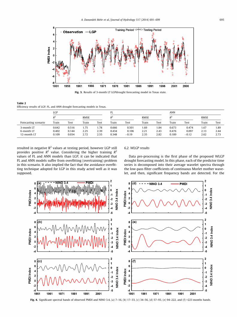
Fig. 3. Results of 3-month LT LGPdrought forecasting model in Texas state.

Table 2Efficiency results of LGP, FL, and ANN drought forecasting models in Texas.

LGP FL ANN

R2 RMSE R2 RMSE R2 RMSE

Forecasting scenario Train Test Train Test Train Test Train Test Train Test Train Test

3-month LT 0.642 0.516 1.75 1.78 0.666 0.501 1.69 1.84 0.673 0.474 1.67 1.896-month LT 0.402 0.144 2.25 2.39 0.434 0.106 2.21 2.43 0.476 0.097 2.13 2.4412-month LT 0.109 0.034 2.72 2.55 0.348 �0.19 2.35 2.82 0.189 �0.12 2.62 2.73

A. Danandeh Mehr et al. / Journal of Hydrology 517 (2014) 691–699 695

resulted in negative R2 values at testing period, however LGP stillprovides positive R2 value. Considering the higher training R2

values of FL and ANN models than LGP, it can be indicated thatFL and ANN models suffer from overfitting (overtraining) problemin this scenario. It also implied the fact that the avoidance overfit-ting technique adopted for LGP in this study acted well as it wassupposed.

Fig. 4. Significant spectral bands of observed PMDI and NINO 3.4, (a) 7–16, (

6.2. WLGP results

Data pre-processing is the first phase of the proposed WLGPdrought forecasting model. In this phase, each of the predictor timeseries is decomposed into their average wavelet spectra throughthe low-pass filter coefficients of continuous Morlet mother wave-let, and then, significant frequency bands are detected. For the

b) 17–33, (c) 34–56, (d) 57–93, (e) 94–222, and (f) >223 months bands.

696 A. Danandeh Mehr et al. / Journal of Hydrology 517 (2014) 691–699

employed data (see Fig. 1), six distinct frequency bands havealready been detected and reported by Özger et al. (2012). The cor-responding time series of wavelet bands obtained by the inversewavelet filtering is given in Fig. 4, showing significant waveletbands of each predictor at time t that are employed as input vari-ables of WLGP at all 3, 6, and 12-month LT scenarios.

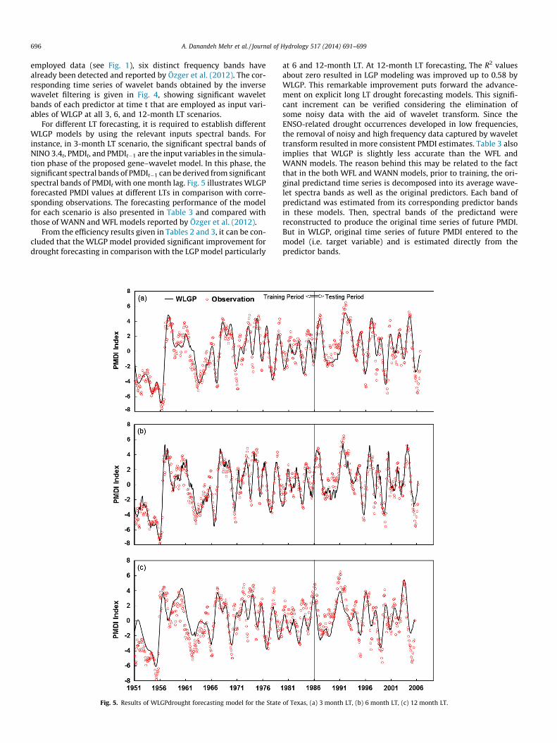
For different LT forecasting, it is required to establish differentWLGP models by using the relevant inputs spectral bands. Forinstance, in 3-month LT scenario, the significant spectral bands ofNINO 3.4t, PMDIt, and PMDIt�1 are the input variables in the simula-tion phase of the proposed gene–wavelet model. In this phase, thesignificant spectral bands of PMDIt�1 can be derived from significantspectral bands of PMDIt with one month lag. Fig. 5 illustrates WLGPforecasted PMDI values at different LTs in comparison with corre-sponding observations. The forecasting performance of the modelfor each scenario is also presented in Table 3 and compared withthose of WANN and WFL models reported by Özger et al. (2012).

From the efficiency results given in Tables 2 and 3, it can be con-cluded that the WLGP model provided significant improvement fordrought forecasting in comparison with the LGP model particularly

Fig. 5. Results of WLGPdrought forecasting model for the State

at 6 and 12-month LT. At 12-month LT forecasting, The R2 valuesabout zero resulted in LGP modeling was improved up to 0.58 byWLGP. This remarkable improvement puts forward the advance-ment on explicit long LT drought forecasting models. This signifi-cant increment can be verified considering the elimination ofsome noisy data with the aid of wavelet transform. Since theENSO-related drought occurrences developed in low frequencies,the removal of noisy and high frequency data captured by wavelettransform resulted in more consistent PMDI estimates. Table 3 alsoimplies that WLGP is slightly less accurate than the WFL andWANN models. The reason behind this may be related to the factthat in the both WFL and WANN models, prior to training, the ori-ginal predictand time series is decomposed into its average wave-let spectra bands as well as the original predictors. Each band ofpredictand was estimated from its corresponding predictor bandsin these models. Then, spectral bands of the predictand werereconstructed to produce the original time series of future PMDI.But in WLGP, original time series of future PMDI entered to themodel (i.e. target variable) and is estimated directly from thepredictor bands.

of Texas, (a) 3 month LT, (b) 6 month LT, (c) 12 month LT.

Table 3Efficiency results of WLGP, WFL and WANN drought forecasting models at Texas.

WLGP WFL WANN

R2 RMSE R2 RMSE R2 RMSE

Prediction scenario Train Test Train Test Train Test Train Test Train Test Train Test

3 month LT 0.847 0.775 1.14 1.22 0.919 0.911 0.83 0.77 0.921 0.867 0.82 0.956 month LT 0.827 0.735 1.21 1.34 0.929 0.896 0.78 0.83 0.928 0.871 0.79 0.9212 month LT 0.661 0.580 1.69 1.67 0.856 0.734 1.10 1.33 0.855 0.764 1.11 1.25

A. Danandeh Mehr et al. / Journal of Hydrology 517 (2014) 691–699 697

6.3. Sensitivity analysis results

It is inevitable that more input variables in evolutionary com-puting methods may lead to more complex formulations(Nourani et al., 2012). Owing to the wavelet filtering, considerablerise in the number of input variables might also magnify predictionerrors (Danandeh Mehr et al., 2013a). Therefore, a genetic-basedsensitivity analysis loop was embedded in the proposed gene–wavelet model, which can be applied during the simulation phase(see Fig. 1). By the aid of this loop, the most effective bands of inputsignificant spectra are distinguished and re-entered to the LGP sys-tem as new input variable sets. The LGP system is performed oncemore for the same target variable and consequently population ofnew programs are generated that might lead the initial model tohigher efficiency.

In order to identify the most effective bands, we considered theexceedance probability of each input band in the thirty best pro-grams evolved by WLGP. Exceedance probabilities of input bandsfor the thirty best WLGP models in terms of frequency were listedin Table 4. The frequency values show what percentage of the bestthirty programs from the model contained the referenced band. Asimilar sensitivity analysis among wavelet decomposed rainfalland runoff time series was also carried out by Nourani et al.(2012) counting the number of selections of each band at fifty GPruns.

According to Table 4, it can be concluded that at 3-month LTforecasting scenario, all input bands contributed in generation of

Table 4Frequency of each band in WLGP Model for PMDI prediction (1.0 = 100%).

Input parameter Band 1 Band 2 Band 3 Band 4 Band 5 Band 6

3 month LT scenarioNINO 3.4 (t) 0.07 0.17 0.2 0.23 0.13 0.47PMDI (t � 1) 0.13 1 0.47 0.2 0.57 0.53PMDI (t) 0.1 1 1 1 0.83 0.33

6 month LT scenarioNINO 3.4 (t) 0.2 0.17 0.3 0.4 0.43 0.4PMDI (t � 2) 0 1 0.77 0.23 0.5 0.3PMDI (t � 1) 0 0.13 0.23 0 0.33 0.17PMDI (t) 0.43 1 1 1 0.93 0.03

12 month LT scenarioNINO 3.4 (t) 0.03 0.5 0.27 0.57 0 0.2PMDI (t � 3) 0 0.83 1 0.63 0.5 0.4PMDI (t � 2) 0 0 0 0.03 0 0.33PMDI (t � 1) 0 0.17 0.27 0.17 0.43 0.2PMDI (t) 0 1 0.5 0.83 0.7 0.07

Table 5Efficiecny results of WLGP model without and with sensitivity analysis.

Prediction scenario WLGP without sensitivity analysis

R2 RMSE

Train Test Train

3 month LT 0.847 0.775 1.146 month LT 0.827 0.735 1.2112 month LT 0.661 0.580 1.69

the best thirty forecasting programs with more or less impact.The bands 2 through 4 of PMDI (t) have the most impact (100%frequency) in the value of PMDI (t + 3). The first, second, and fifthbands of NINO 3.4 have the least impacts (less than 20% frequency)in this scenario.

At 6-month LT forecasting scenario, PMDI (t) and PMDI (t � 2)have the most impact, respectively and NINO 3.4 bands are moreeffective than those of PMDI (t � 1). The bands 2 through 4 of PMDI(t) are the most effective bands in prediction of PMDI (t + 6) as wellas PMDI (t + 3). The bands 3 through 5 of NINO 3.4 (t) show signif-icant increment in prediction of 6-month LT drought in comparisonwith corresponding bands at 3-month LT. Such a comparativesignificant increment is also observed at 12-month LT forecastingscenario among the bands 2 through 4 of NINO 3.4 (t) and corre-sponding bands in 3-month LT. It implies the high potential effectof the NINO 3.4 (t) index in 6-month through 12-month LT droughtforecasting. Details on physical mechanism behind the fact thatENSO events are correlated with drought conditions in Gulf ofMexico region can be found in the literature (e.g., Kahya andDracup, 1993, 1994; Dracup and Kahya, 1994; Piechota andDracup, 1996; Rajagopalan et al., 2000). As given in the captionfor Fig. 4, significant spectral bands of NINO 3.4 values at the bands3 and 4 represent the 34–56 and 57–93-month spectrums, respec-tively. In other words, these bands roughly represent 3–8 yearspectrums that are more or less equal to the prevalent frequencyof ENSO events. It implies mid to long range forecasting potentialof NINO 3.4 index that is consistent with results of the study con-ducted by Piechota and Dracup (1996). As it was mentioned previ-ously, a strong relationship between dry condition and La Niñaevents in the State of Texas has been reported by Piechota andDracup (1996). The authors pointed out that significant PDSIrelated La Niña signal appeared to be even negative during theperiod starting from November of event year continuing by theend of the following year. It is also important to emphasize thatthe magnitude of these negative PDSI anomalies in GM1 regionwere the largest among all regions in their study domain. Thisshows that the impacts of La Niña events on the PDSI pattern arelong lasting in the Texas area implying a mid to long rangeforecasting potential.

Based upon frequency of input bands tabulated in Table 4, thebands possessing less than 50% frequency at the best thirty pro-grams were eliminated from input variables of simulation phaseof WLGP (see Fig. 1) and the rest of the bands spectra consideredin re-performing of the WLGP as the effect of sensitivity analysisloop. For example, the NINO3.4 index does not have any band withmore than 50% frequency at 3 and 6-month LT scenarios (see

WLGP with sensitivity analysis

R2 RMSE

Test Train Test Train Test

1.22 0.841 0.761 1.16 1.261.34 0.804 0.686 1.28 1.461.67 0.770 0.642 1.39 1.54

698 A. Danandeh Mehr et al. / Journal of Hydrology 517 (2014) 691–699

Table 4). Thus, none of the NINO 3.4 bands entered in re-performingthe model for 3 and 6-month LT forecasting. However its second andfourth bands are considered in model re-performing 12-month LT.

The efficiency results of the WLGP model with the effect ofsensitivity analysis for drought forecasting in the State of Texaswith 3, 6, and 12-month LT were presented in Table 5 and werecompared with those of WLGP without considering the sensitivityanalysis loop. It is evident from the table that the use of sensitivityanalysis generated more accurate forecasts of PMDI only in12-month LT scenario. It indicates that: (i) The uncertainty featureof our data (noise) is formerly well diminished at 3 and 6-month LTforecasting due to the wavelet transform, (ii) increasing in thenumber of input sub-signals in 12-month LT scenario may magnifyprediction errors and lead to unreliable outputs unless sensitivityanalysis has been employed, and (iii) There is a strong potentialin NINO 3.4 index to forecast drought with one year LT.

7. Conclusions

In this study, the LGP and wavelet transform concepts werecombined to develop an explicit hybrid gene–wavelet model,WLGP for long LT drought forecasting using PMDI and NINO 3.4values as predictors and forthcoming PMDI index as a predictand.The model is capable: (i) to obtain the average wavelet spectra, (ii)to detect the significant spectral bands (iii) to forecast future PMDI,and (iv) to optimize the number of significant spectral bands via itsheuristics-based sensitivity analysis feature. The application of theWLGP across the State of Texas provided significant improvementin accuracy over the ad hoc LGP models particularly at 6 and 12-month LT forecasting. Sensitivity analysis among input variablebands indicated that the preceding values of PMDI have higherimpact than NINO 3.4 for drought forecasting up to 6-month LT,whereas the latter has high potential to forecast drought for 6through 12-month LT.

As a suggestion for future research, with the aid of the proposedmodel, other climatic indices impacts on drought condition can beinvestigated. The model also can be used to investigate the effec-tiveness of NINO 3.4 and PMDI indices in order to predict droughthaving LTs longer than a year. In this study, we used a fixed motherwavelet (Morlet wavelet functions) to decompose our input timeseries. Effect of different wavelet functions may be considered asa way to optimize the current model in future studies.

References

Aytek, A., Kisi, O., 2008. A genetic programming approach to suspended sedimentmodelling. J. Hydrol. 351 (3–4), 288–298.

Bacanli, U.G., Firat, M., Dikbas, E.F., 2009. Adaptive neuro-fuzzy inference system fordrought forecasting. Stoch. Environ. Res. Risk Assess. 23, 1143–1154.

Banzhaf, W., Nordin, P., Keller, R. and Francone, F.D., 1998. Genetic programming-anintroduction on the automatic evolution of computer programs and itsapplication. dpunkt/Morgan Kaufmann: Heidelberg, San Francisco.

Barros, A.P., Bowden, G., 2008. Toward long-lead operational forecasts of drought:an experimental study in the Murray-Darling River Basin. J. Hydrol. 357 (3–4),349–367.

Belayneh, A., Adamowski, J., 2012. Standard precipitation index drought forecastingusing neural networks, wavelet neural networks, and support vector regression.Appl. Comput. Intell. Soft Comput. Article ID 794061, 13pages.

Belayneh, A., Adamowski, J., Khalil, B., Ozga-Zielinski, B., 2014. Long-term SPI droughtforecasting in the Awash River Basin in Ethiopia using wavelet neural networkand wavelet support vector regression models. J. Hydrol. 508, 418–429.

Bogradi, I., Matyasovsky, I., Bardossy, A., Duckstein, L., 1994. A hydroclimotologicalmodel of arial drought. J. Hydrol. 153, 245–264.

Cancelliere, A., Mauro, G.D., Bonaccorso, B., Rossi, G., 2007. Drought forecastingusing the standardized precipitation index. Water Resour. Manage 21, 801–819.

Danandeh Mehr, A., Kahya, E., Olyaie, E., 2013a. Streamflow prediction using lineargenetic programming in comparison with a neuro-wavelet technique. J. Hydrol.505, 240–249.

Danandeh Mehr, A., Kahya, E., Bagheri, F., Deliktas, E. 2013b. Successive-stationmonthly streamflow prediction using neuro-wavelet technique. Earth Sci.Inform., doi: 10.1007/s12145-013-0141-3, in press.

Dolling, O.R., Varas, E.A., 2002. Artificial neural networks for streamflow prediction.J. Hydraul. Res. 40 (5), 547–554.

Dorado, J., Rabuñal, J.R., Pazos, A., Rivero, D., Santos, A., Puertas, J., 2003. Predictionand modeling of the rainfall-runoff transformation of a typical urban basinusing ANN and GP. Appl. Artif. Intell. 17, 329–343.

Dracup, J.A., Kahya, E., 1994. The relationships between U.S. streamflows and LaNina events. Water Resour. Res. 30, 2133–2141.

Fernandez, C., Vega, J.A., Fonturbel, T., Jimenez, E., 2009. Streamflow drought timeseries forecasting: a case study in a small watershed in North West Spain. Stoch.Environ. Res. Risk Assess. 23, 1063–1070.

Francone, F.D., 2010. DiscipulusTM with Notitia and solution analytics owner’smanual. Register Machine Learning Technologies Inc., Littleton, CO, USA.

Ghorbani, M.A., Khatibi, R., Aytek, A., Makarynskyy, O., Shiri, J., 2010. Sea water levelforecasting using genetic programming and artificial neural networks. Comput.Geosci. 36 (5), 620–627.

Heim Jr., Richard R., 2002. A review of twentieth-century drought indices used inthe United States. Bull. Amer. Meteor. Soc. 83, 1149–1165.

Kahya, E., Dracup, J.A., 1993. US streamflows patterns in relation to the El Nino/Southern Oscillation. Water Resourc. Res. 29, 2491–2503.

Kahya, E., Dracup, J.A., 1994. The influence of type I EI Nino and La Nina events onstreamflows in the Pacific Southwest of the United States. J. Clim. 7 (6),965–976.

Kim, T.W., Valdes, J.B., 2003. Nonlinear model for drought forecasting based on aconjunction of wavelet transforms and neural networks. J. Hydrol. Eng. 8 (6),319–328.

Kis�i, Ö., 2008. Stream flow forecasting using neuro-wavelet technique. Hydrol.Process. 22, 4142–4152.

Kisi, O., Guven, A., 2010. Evapotranspiration modeling using linear geneticprogramming technique. J. Irrig. Drain. Eng. 136 (10), 715–723.

Koza, J.R., 1992. Genetic programming: on the programming of computers by meansof natural selection. MIT Press, Cambridge, MA, USA.

Labat, D., 2005. Recent advances in wavelet analyses: Part 1. A review of concepts. J.Hydrol. 314 (1–4), 275–288.

Labat, D., Ababou, R., Mangin, A., 2000. Rainfall–runoff relations for karstic springs.Part II: continuous wavelet and discrete orthogonal multiresolution analyses. J.Hydrol. 238, 149–178.

Lohani, V.K., Loganathan, G.V., 1997. An early warning system for droughtmanagement using the Palmer drought index. J. Am. Water Res. Assoc. 33 (6),1375–1386.

Mallat, S., 1998. A Wavelet Tour of Signal Processing, 2nd Ed. Academic Press, SanDiego, CA.

Mishra, A.K., Desai, V.R., 2005. Drought forecasting using stochastic models. J. Stoch.Environ. Res. Risk Assess. 19, 326–339.

Mishra, A.K., Desai, V.R., 2006. Drought forecasting using feed forward recursiveneural network. Ecol. Model. 198, 127–138.

Mishra, A.K., Singh, V.P., 2010. A review of drought concepts. J. Hydrol. 391 (1–2),202–216.

Mishra, A.K., Singh, V.P., 2011. Drought modelling – a review. J. Hydrol. 403,157–175.

Mishra, A.K., Desai, V.R., Singh, V.P., 2007. Drought forecasting using a hybridstochastic and neural network model. J. Hydrol. Eng. 12 (6), 626–638.

Modarres, R., 2007. Streamflow drought time series forecasting. Stoch. Environ. Res.Risk Assess. 15 (21), 223–233.

Morid, S., Smakhtin, V., Bagherzadeh, K., 2007. Drought forecasting using artificialneural networks and time series of drought indices. Int. J. Climatol. 27 (15),2103–2111.

Nourani, V., Alami, M.T., Aminfar, M.H., 2009a. A combined neural-wavelet modelfor prediction of Ligvanchai watershed precipitation. Eng. Appl. Artif. Intell. 22(3), 466–472.

Nourani, V., Komasi, M., Mano, A., 2009b. A multivariate ANN wavelet approach forrainfall–runoff modelling. Water Resour. Manage 23, 2877–2894.

Nourani, V., Kisi, O., Komasi, M., 2011. Two hybrid artificial intelligence approachesfor modeling rainfall–runoff process. J. Hydrol. 402, 41–59.

Nourani, V., Komasi, M., Alami, M.T., 2012. Hybrid wavelet–genetic programmingapproach to optimize ANN modelling of rainfall-runoff process. J. Hydrol. Eng. 7(6), 724–741.

Nourani, V., Hosseini Baghanam, A., Adamowski, J., Gebremichael, M., 2013a. Usingself-organizing maps and wavelet transforms for space–time pre-processing ofsatellite precipitation and runoff data in neural network based rainfall–runoffmodeling. J. Hydrol. 476, 228–243.

Nourani, V., Komasi, M., Alami, M.T., 2013b. Geomorphology-based geneticprogramming approach for rainfall-runoff modeling. J. Hydroinform. 15 (2),427–445.

Nourani, V., Hosseini Baghanam, A., Adamowski, J., Kisi, O., 2014. Applications ofhybrid Wavelet-Artificial Intelligence models in hydrology. A review. J. Hydrol.514, 358–377.

Onderka, M., Banzhaf, S., Scheytt, T., Krein, A., 2013. Seepage velocities derived fromthermal records using wavelet analysis. J. Hydrol. 479, 64–74.

Özger, M., 2010. Significant wave height forecasting using wavelet fuzzy logicapproach. Ocean Eng. 37 (16), 1443–1451.

Özger, M., Mishra, A.K., Singh, V.P., 2009. Low frequency drought variabilityassociated with climate indices. J. Hydrol. 364 (1–2), 152–162.

Özger, M., Mishra, A.K., Singh, V.P., 2012. Long lead time drought forecastingusing a wavelet and fuzzy logic combination model. J. Hydrometeorol. 13,284–297.

A. Danandeh Mehr et al. / Journal of Hydrology 517 (2014) 691–699 699

Partal, T., Kis�i, Ö., 2007. Wavelet and neuro-fuzzy conjunction model forprecipitation forecasting. J. Hydrol. 342 (1–2), 199–212.

Pesti, G., Shrestha, B., Duckstein, L., Bogardi, I., 1996. A fuzzy rule-based approach todrought assessment. Water Resour. Res. 32 (6), 1741–1747.

Piechota, T.C., Dracup, J.A., 1996. Drought and regional hydrologic variation in theUnited States: associations with the El Niño–Southern Oscillation. WaterResour. Res. 32 (5), 1359–1373.

Pongracz, R., Bogardi, B., Duckstein, L., 1999. Application of fuzzy rule-basedmodeling technique to regional drought. J. Hydrol. 224, 100–114.

Poli, R., Langdon, W.B. and McPhee, N.F., 2008. A Field Guide to GeneticProgramming. Published via http://lulu.com and freely available at http://www.gp-field-guide.org.uk (With contributions by J.R. Koza)

Rabuñal, J.R., Puertas, J., Suárez, J., Rivero, D., 2007. Determination of the unithydrograph of a typical urban basin using genetic programming and artificialneural networks. Hydrol. Process., 476–485.

Rajagopalan, B., Cook, E., Lall, U., Ray, B.K., 2000. Spatiotemporal variability of ENSOand SST teleconnections to summer drought over the United States during thetwentieth century. J. Clim. 13, 4244–4255.

Rao, A.R., Padmanabhan, G., 1984. Analysis and modeling of palmer’s drought indexseries. J. Hydrol. 68, 211–229.

Sen, Z., 1990. Critical drought analysis by second order Markov chain. J. Hydrol. 120,183–202.

Webster, P.J., Hoyos, C.D., 2004. Prediction of monsoon rainfall and river dischargeon 15–30-day time scales. Bull. Am. Meteorol. Soc. 85 (11), 1745–1765.

Whigham, P.A., Crapper, P.F., 2001. Modelling rainfall-runoff using geneticprogramming. Math. Comput. Model. 33, 707–721.

Wu, C.L., Chau, K.W., Li, Y.S., 2009. Methods to improve neural network performancein daily flows prediction. J. Hydrol. 372, 80–93.