Journal - Home | Association of Agrometeorologists

Journal of

Agrometeorology

Volume 22 Special Issue June, 2020

Association of AgrometeorologistsAnand-388 110, India

Published by Association of Agrometeorologists (Delhi Chapter), India Meteorological Department, Lodhi Road, New Delhi-110003, India and printed at Quick Digital Print Services, Kotla Mubarakpur, New Delhi, India.

Journ

al o

f Agro

mete

oro

logy

Volu

me 2

2 S

pecia

l Issue J

un

e, 2

020

GLIMPSES OF - 2019INAGMET GLIMPSES OF - 2019INAGMET

Journal of

Agrometeorology


Volume 22 Special Issue June 2020

Executive Council (2019-21)

President Dr. Vyas Pandey, AAU, AnandEx-Officio member Dr. Akhilesh Gupta, DST, New DelhiVice Presidents Dr. J. D. Jadhav, MPKV, Pune Dr. S. K. Bal, CRIDA, HyderabadSecretary Dr. S. B. Yadav, AAU, AnandJt. Secretary Dr. A. K. Shrivastava, JNKVV, Tikamgarh, MP Treasurer Dr. B. I. Karande, AAU, AnandMembers Dr. N. Subash, ICAR-IIFSR, Meerut Dr. C. S. Dagar, CCS HAU, Hisar Dr. S. Sridhara, UAHS, Shimoga Dr. Sandeep S. Sandhu, PAU, Ludhiana Dr. K. K.Dakhore, VNMKV, Parbhani Co-opted members Dr. N. R. Patel, IIRS/ISRO, Dehradun Dr. Kamaljit Ray, MoBS, New DelhiZonal membersNorth Zone Dr. R. H. Kanth, SKUAST-K, Kashmir West Zone Shri V. B. Vaidya, AAU, AnandCentral Zone Dr. R. K. Mall, BHU, VaranasiEast Zone Dr. Abdus Sattar, RPCAU, Pusa, BiharSouth Zone Dr. B. Ajith Kumar, KAU, Thrissur

Chapters Chairman Chapters ChairmanHisar Dr. Raj Singh Coimbatore Dr S. PanneerselvamLudhiana Dr. Prabhjyot Kaur New Delhi Dr. K.K.SinghHyderabad Dr. P. Vijayakumar Jammu Dr. B.C. SharmaPune Shri S. C. Badwe Faizabad Dr. Padmakar TripathiMohanpur Dr. Lalu Das Raipur Dr. G.K. DasPantnagar Dr. R. K. Singh Thrissur Dr. Ajith K.

ASSOCIATION OF AGROMETEOROLOGISTS(Regd. No. GUJ/1514 I Kheda Dt. 22/3/99)

Anand Agricultural University, ANAND - 388 110, India.E-mail: [email protected]

Website : http://www.agrimetassociation.org

AAM- Delhi ChapterChairman : Dr. K.K. Singh, IMD, New Delhi

Secretary : Dr. D.K. Das, ICAR-IARI, New Delhi

Treasurer : Dr. Shalini Saxena, MNCFC, New Delhi

Journal of Agrometeorology(ISSN 0972 - 1665)

Journal of Agrometeorology is a quarterly publication appearing in March, June, September and December. It is indexed and abstracted in several indexing agencies such as AGRICOLA, Current Content, CAB International, SciSearch, Journal Citation Report, Indian Science Abstract (ISA), INSDOC, SCOPUS, Elsevier publication, ProQuest, EBSCO, Scimago, Bioxbio, SCIJOURNAL, Resurchify and many others. It is rated as 6.56 by NAAS in year 2019.

Editorial BoardEditor-in-Chief

B.V. Ramana Rao, Hyderabad

E-mail: [email protected]

Managing Editor

Dr. Santanu Kumar Bal, ICAR-CRIDA, Hyderabad


International Editor

Dr. M. V. K. Sivakumar, Geneva, Email: [email protected]

Editors

Dr. P. Vijaya Kumar, Central Research Institute for Dryland Agriculture, Hyderabad

Dr. K.K. Singh, India Meteorological Department, New Delhi

Dr. Gauranga Kar, Indian Institute of Water Management, Bhubaneswar

Dr. N.R. Patel, Indian Institute of Remote Sensing, Dehradun

Dr. R.K. Mall, Varanasi Hindu University, Varanasi

Dr. M. Srinivas Rao, Central Research Institute for Dryland Agriculture, Hyderabad

Dr. S. Desai, Central Research Institute for Dryland Agriculture, Hyderabad

Dr. N. Subash, Indian Institute of Farming System Research, Modipuram

Dr. M.K. Nanda, Bidhan Chandra Krishi Vidyapeeth, Mohanpur

Dr. Lalu Das, Bidhan Chandra Krishi Vidyapeeth, Mohanpur

Dr. V. Sejian, National Institute of Animal Nutrition and Physiology, Bangalore

International Symposium on “ADVANCES IN AGROMETEOROLOGY FOR

MANAGING CLIMATIC RISKS OF FARMERS” (INAGMET-2019)

Patrons

Shri S.K. Pattanayak, Secretary, MoAg& FWDr T. Mohapatra, Secretary, DARE & DG, ICARDr M. Rajeevan, Secretary, Ministry of Earth SciencesProf. Ashutosh Sharma, Secretary, DST

Shri U.P. Singh, Secretary, MoWR, RD & GR Dr. Renu Swarup, Secretary, Dept. of BiotechnologyDr K. Sivan, Secretary, DoSand Chairman, ISROShri C.K. Mishra, Secretary, MoEF&CC

International Advisory Committee (IAC)Convener:

Dr Akhilesh Gupta, President, AAM& Adviser, DSTMembers:

Dr Byong Lee, President, CAgM, WMODr David Bergvinson, DG, ICRISATDr Sansul Huda, AustraliaProf Roger Stone, AustraliaDr Orivaldo Brunini, BrazilDr Jim Saligner, New ZealandDr Federica Rossi, ItalyDr Alexender Kleshchenko, RussiaDr Raymond Motha, USADr Richard Allen, Univ. of IdahoDr Neale Christopher, Univ. of NebraskaDr M.V.K. Sivakumar, WMODr Rupa Kumar Kolli, WMOProf J. Shukla, George Mason University, USADr A. Subbaiyah, RIMES, Bangkok

Dr Panjab Singh, President, NAAS Dr Mangala Rai, Former DG, ICARDr P.K. Aggarwal, CCAFSDr Rama Nemani, NASA, USADr V.K. Dadhwal, Director, IISTDr Shyam Khadka, FAODr M.C. Varshney, Former VC, AAUDr L.S. Rathore, World BankDr Y.S. Ramakrishnan, Member, NADM, New DelhiDr S.S. Hundal, LudhianaDr ASRAS Shastri, RaipurDr O.P. Bishnoi, HisarProf B.V. RamanaRaoDr A.M. Shekh, AnandDr T.N. Balasubramanian, Coimbatore

National Organizing Committee (NOC)Chairman: Dr K.J. Ramesh, DG, IMD

Co-Chairs: Dr A.K. Singh, Director, IARIDr Akhilesh Gupta, President, AAM

Conveners:Dr VyasPandey, Secretary, AAM, Anand

Dr K.K. Singh, Chairman, AAM Delhi ChapterMembers:

Prof S.K. Dash, President, IMS, New DelhiDr Tapan Misra, Director, SAC, AhmedabadDr Ravi Shankar Nanjundiah, Director, IITM, PuneDr Neeta Verma, DG, NIC, New DelhiDr A.K. Singh, DDG, Agri. Extn, ICAR, New DelhiDr K. Alagusundaram, DDG, NRM, ICAR, New DelhiDr Santanu Chowdhury, Director, NRSC, HyderabadDr Prakash Chauhan, Director, IIRS, DehradunDr Harsh Kumar Bhanwala, Chairman, NABARDDr G.S. Jha, Chairman, CWC, New DelhiDr K.C. Naik, Chairman, CGWB, New DelhiProf. Satish Chandra Garkoti, JNUA.L. Ramanathan, JNUDr Surendra Kumar Singh, Director, NBSS & LUPDr K. Sammi Reddy, Director, CRIDA, Hyderabad Dr V. Usha Rani, DG, MANAGE, Hyderabad Dr S..Pasupalak, VC, OUAT, BhubaneswarDr Chiratan Chattopadhyay, VC, UBKV, PundibariDr R.C. Srivastava, VC, RPCAU, PusaDr B. Venkateswarulu, VC, MAU, ParbhaniDr Rajiv Kumar Tayal, Secretary, SERB, New DelhiMs Upma Srivastava, AS, DAC & FW Dr E.N. Rajagopal, Head, NCMRWF, NOIDAShri GopalIyengar, Advisor, MoES, New Delhi

Dr M. Mohapatra, Scientist ‘G’, IMDDr Bhoop Singh, Adviser, DST, New DelhiDr Himanshu Pathak, Director, NRRI, CuttackDr D Rajireddy, PJTSAU, HyderabadDr VUM Rao, AAM, HyderabadDr P Vijayakumar, CRIDA, HyderabadDr GourangKar, WTCER, Bhubaneswar Dr Surender Singh, AAM, HisarDr J.D. Jadhav, AAM, SolapurDr B. Ajith Kumar, AAM, TrichurDr Mahender Singh, AAM, JammuDr S.S. Sandhu, AAM, LudhianaDr Rucha Dave, AAM, AnandDr Rani Saxena, AAM, JaipurDr K.K. Dakhore, AAM, ParbhaniDr V.Geethalakshmi, AAM, MaduraiDr U.S. Sakia, AAM, BarapaniDr S.K. Bal, AAM, HyderabadDr K.K. Agarwal, AAM, JabalpurDr R.S. Rana, AAM, PalampurDr Prabhjyoti Kaur Sidhu, AAM, LudhianaDr S. Panneerselvam, AAM, CoimbatoreDr Lalu Das, AAM, MohanpurDr B.K. Singh, BKS Weather Sys, NOIDA

Felicitation and Honours

Fellow• DrASNain,GBPUAT,Pantnagar

• DrSKBal,ICAR-CRIDA,Hyderabad

Awardees• DrS.VenkataramanYoungScientistAward-2019

• DrKKDakhore,VNMKV,Parbhani

• DrP.D.MistryAwardforbestPhDthesisinAgril.Meteorology

• DrBIKarande

• Prof.PSNSastryAward-2019forBestMScthesisinAgril.Meteorology

• MrRamnarayanSingh

• Prof.B.V.Ramanaraobestpaperaward-2019

• DrPRaja

JAM best papers• ChitraShukla

• AbdulNiyas

• SKJalota

Winning presentationsa) Oral Sessions• ImpactofweathervariablesonyieldofPearlMillet(Pennisetum glaucum) under

different growing environments in scarcity zone ofMaharashtra- V.M. Londe,K.K. Chavan, J.D. Jadhav and P.B. Pawar

• ConditionalProbabilityforRainfallAnalysisofWetandDrySpellforCropPlanningunder differentAgro climatic Zone of JammuRegion-MahenderSingh,CharuSharma, B.C. Sharma, Vishav Vikas, R.K. Srivastava, Sushmita M. Dadhich, J.P. Singh and Hemant Dadhich

• Assessment of wheat production scenario under projected climate change inRanchi region of Jharkhand-PragyanKumari,A.WadoodandRajnishPrasadRajesh

• RicecropdamageassessmentinSrikakulam,AndhraPradesh,IndiapostcycloneTitli(October2018)usingSARremotesensingandORYZAcropgrowthmodel-

Sushree Satapathy, Emma Quicho, Ponnurangam Ganesan, Aileen Maunahan, Luca Gatti, Gene Romuga, Cornelia Garcia, Prabhu Prasadini, Prasuna Rani Podila, Sunil Kumar Medida, Kranthi Kumar Challa, Ramohan K.J. Reddy, Tri Setiyono, Francesco Holecz

• IntercomparisonofsevenTemperature-HumidityindexequationstofindoutbestTHIforcentralzoneofKerala-HarithalekshmiV.,Aswathi,K.P.,B.Ajithkumar

b) Short-Oral Sessions• EvaluatingtheperformanceofCMIP5GCMsoversixagro-climaticzonesofWest

Bengalusingconventionalstatisticalindices-SayaniBhowmickandLaluDas

• SpatialandtemporalvariabilityanalysisofrainfallformajorjutegrowingdistrictsofWestBengal-TaniaBhowmick,DBarban,Nmalam,RSaha,SRoy,SikhasriDas, Abhishek Bagui, Priyanka Chakravarty and Prantapratim Banerjee

• Validationofcropsimulationmodelatmicro-levelusingcropcuttingexperimentfor wheat yield in Uttar Pradesh-Akanksha Das, Yogesh Kumar, K.K. Singh,Shibendu S Ray, S D Attri, A.K.Baxla and Priyanka Singh

• Mapping of groundwater quality for suitability of climate resilient farming inEastern Agroclimatic zone of Haryana, India-Ram Prakash, Satyavan, SanjayKumar and Surender Singh

• Management of Rhizome Rot Disease of Ginger through Adjustment of CropMicroclimateinNorthBankPlainZone-PrasanthaNeog,D.Saikia,R.K.Gswamiand R. R.Changmai

c) Poster Sessions• FruitdroppatternandphenologicalbehaviourunderaridirrigatedzoneofPunjab

inKinnowmandarin-AKSangwan,MKBatth,PKArora,AshwinKaur,SandeepRaheja and Sashi Pathania

• Performance of Indian mustard cultivars in varying sowing conditions undersouth western Punjab-Sudhir Kumar Mishra, Gurpreet Singh, Kulvir Singh,Kuldeep Singh and Pankaj Rathore

• Role of micrometeorological and agrometeorological variables in forecastingof Alternaria leaf spot in soybean at Dharwad in northern transition zone of Karnataka-AmithG,VenkateshHandShamaraoJahagirdar

• IdentificationofEfficientCroppingZoneandadjustingsowingwindowforgreengram in Tamil Nadu-C. Arulmathi, S. Kokilavani, S. Panneerselvam and Ga.Dheebakaran

• Weather parameters influencing biochemical constituents in Asiatic cotton(Gossypium arboreumL.)-Sunayana,R.S.Sangwan,M.L.KhicharandManpreetSingh

Journal of AgrometeorologyVolume 22 special issue June 2020

Contents

Foreword

Message

CH. SRIDEVI, K. K. SINGH, P. SUNEETHA, S. C. BHAN, ASHOK KUMAR, V.R.DURAI, ANANDK.DAS, LATAVISHNOI&M.RATHI -Location specific weather forecast from NWP Models using different statisticaldownscalingtechniquesoverIndia

1-8

P. RAJA K. RAJAN, P. MAHESH, K. KANNAN, U. SURENDRAN, K.MALLIKARJUNO.P.SKHOLAANDC.ARULMATHI-Study on CO2 and CH4 emissions from the soils of various land use systems in temperate mountainous ecosystem of part of Nilgiris, Western Ghats, India

9-14

JATINDER KAUR, PRABHJYOT KAUR AND SAMANPREET KAUR -Analyzing uncertainties amongst the seventeen GCMs for prediction of temperature, rainfall and solar radiation in central irrigated plains in Punjab

15-23

MAHENDER SINGH, CHARU SHARMA, B.C. SHARMA, R.K. SRIVASTAVA, SUSHMITAM. DADHICH, J.P. SINGH AND VIKAS GUPTA -Rainfall probability analysis for crop planning of Jammu region

24-32

G. B. GOHAIN, K.K. SINGH, R.S. SINGH, PRIYANKA SINGH - Regional CropYieldEstimationSystem (RCYES)usingacropsimulationmodelDSSAT V4.7: concept, methods, development, and validation

33-38

BAVISH, S, GEETHALAKSHMI, V, KOKILAVANI, S, GOWTHAM, R, BHUVANESWARI, K, AND RAMANATHAN, SP. -DelineationofEfficientCropping Zone for Onion over Tamil Nadu

39-42

K. K. DAKHORE, A. KARUNAKAR, J. D. JADHAV Y.E KADAM, D. P.WASKARANDP. VIJAYAKUMAR -Analysis of Drought in the Maharashtra by Using the Standardized Precipitation Index

43-50

JASTI VENKATA SATISH ANDB. AJITHKUMAR - “Assessment of rice (Oryza sativa L.) productivity under different climate change scenarios”

51-59

VENNILA S, SHABISTANA NISAR, MURARI KUMAR, YADAV SK, PAUL RK, SRINIVASARAOMANDPRABHAKARM-Impact of Climate Variability on Species Abundance of Rice Insect Pests across Agro Climatic Zones of India

60-67

PRAGYAN KUMARI, A.WADOOD AND RAJNISH PRASAD RAJESH -Assessment of wheat production under projected climate scenario in Ranchi region of Jharkhand

68-75

M.L. KHICHAR, RAM NIWAS, ANIL KUMAR, RAJ SINGH AND S.C. BHAN -Weather based decision support system for crop risk management

76-79

MAHENDER SINGH, CHARU SHARMA, B.C. SHARMA, VISHAW VIKAS ANDPRIYANKASINGH-Weather based yield prediction model at various growth stages of wheat crop in different Agro Climatic Zones of Jammu region

80-84

ABDUSSATTAR,S.A.KHANANDGULABSINGH-Evaluation of actual evapotranspiration, water surplus and water deficit for climate smartrainfed crop planning in Bihar

85-89

AKSANGWAN,MKBATTH,PKARORAANDSANDEEPRAHEJA-Fruit drop pattern and phenological behavior under arid irrigated zone of PunjabinKinnowmandarin(Citrus reticulata L.).

90-97

VENGATESWARI M, GEETHALAKSHMI V, BHUVANESWARI K, PANNEERSELVAM S - Sustaining rainfed maize productivity under varied ENSO events in Tamil Nadu

98-103

BARUN BISWAS AND JAGDISH SINGH - Assessing yield-weatherrelationships in kharif maize under Punjab conditions using data mining method

104-111

NAVNEET KAUR, KK GILL, BALJIT SINGH, RIS GILL AND BHADRA PARIJA-HeatUnitRequirementandRadiationUseEfficiencyofWheatCultivars under Agroforestry Systems in Northern India

112-120

R.RENGALAKSHMI, V.GEETHALAKSHMIANDK.BHUVANESWARI -Spatial variation of rainfed maize yield response to climate change in Tamil Nadu

121-125

D.T. MESHRAM, K.D. BABU, A.K. NAIR, P. PANIGRAHI AND S.S. WADNE - Response of Pomegranate (Punica granatum L.) to deficit irrigationsystemunderfieldconditions.

126-135

RAGHAVENDRA ACHARI, H. VENKATESH AND HIREMATH, J.R. -

Farmers’ Preparedness to manage Grape Diseases through Agromet Advisories based on Weather based Forecast Models

136-140

PANKAJ DAHIYA, EKTA PATHAK MISHRA, BISWARUP MEHRA, ABHILASH, SURESH, M.L. KHICHAR AND RAM NIWAS - Impact of Climatic Variability on Wheat Yield in Indian Subcontinent

141-148

DIVYA, K K GILL, S S SANDHU, SAMANPREET KAUR, SS WALIA AND MAMTA RANA - Assessing the performance of wheat cultivars under present and futuristic climatic conditions using DSSAT model

149-154

S.S.SANDHU,PRABHJYOT-KAURANDK.K.GILL-Change in timing of occurrence of temperature extremes in central Punjab

155-162

SHARANAPPA KURI, SHIVARAMU, H. S, THIMMEGOWDA, M. N., YOGANANDA,S.B.,PRAKASH,S.S.ANDMURUKANNAPPA-Water Use EfficiencyofPigeonpeaVarietiesunderVariedDatesofSowingandRowSpacingunderrainfedAlfisolsofKarnataka

163-169

VIKAS GUPTA, MEENAKSHI GUPTA, MAHENDER SINGH AND B. C. SHARMA - Thermal requirement for phenophases and yield of wheatvarietiesundervarioussowingenvironmentsandnitrogenlevelsinsub-tropical region of Jammu

170-177

BHAGAT SINGH, MUKESH KUMAR, A.K. DHAKA AND RAJ SINGH -Response of Wheat Genotypes to different sowing times in relation to Thermal Environments in Haryana

178-185

POOJA, RAJENDER SINGH, S.S. DHANDA, N.R. YADAV - Effect of MeteorologicalParametersonStripeRust(Puccinia striformis f. sp. tritici) ofWheat(Triticum aestivum L. emThell)

186-191

RANU PATHANIA, RAJENDRA PRASAD, RANBIR SINGH RANA, SUDHIR KUMARMISHRAANDSAURAVSHARMA-Calibration and validation of CERES-wheatmodelforNorthWesternHimalayas

192-196

S. V. PHAD, K. K. DAKHORE, R. S. SAYYAD, NITESH AWASHTHI AND R. BALASUBRAMANIAM-EstimationofReferenceEvapotranspiration(ETo)andCropWaterRequirementofSoybeanandCottonForMarathwadaRegion

197-203

R.REJANI, K.V. RAO, D. KALYANA SRINIVAS, K. SAMMI REDDY, G.R. CHARY, K.A. GOPINATH, M.OSMAN, R.S. PATODE AND M.B. NAGDEVE -Spatial and temporal variation in the runoff potential and irrigation requirementofcropsunderchangingclimaticscenariosintheWesternVidarbha zone in Maharashtra

204-209

RAMPRAKASH,SANJAYKUMAR,SATYAVANANDSURENDERSINGH-MappingofgroundwaterqualityforsuitabilityofclimateresilientfarmingintheEasternagro-climaticzoneofHaryana,India

210-217

KAVITA BHATT, K. K. GILL AND MAMTA RANA - Pre-Harvest YieldPrediction of Mustard in Central Punjab using InfoCrop Model

218-223

RAJKUMARPAL-Impact of varying nitrogen levels on seed cotton yield usingCROPGRO-cottonmodelforSouth-WesternregionofPunjab

224-228

K.K.GILL,SATINDERKAUR,S.S.SANDHUANDS.S.KUKAL-Evaluation of real time weather related fluctuations and wheat productivity innorthern India

229-234

MAMTA, RAJ SINGH, SURENDER SINGH, DIWAN SINGH, ANIL KUMAR, DIVESH, ABHILASH AND AMIT - Annual trends of temperature and rainfallextremesinHaryanafortheperiod1985-2014,India

235-242

N. MANIKANDAN, P. PANIGRAHI, S. PRADHAN, S. K. RAUTARAY AND G. KAR-Evaluatingminipanevaporimeterforon-farmirrigationscheduling

243-247

HARITHARAJS.ANDB.AJITHKUMAR-Crop planning based on water balance approach in Kerala

248-250

Y. E. KADAM; K. K. DAKHORE; A. S. JADHAV; D. P. WASKAR ; P. VIJAYA KUMARANDNITESHAWASTHI-Impact of El Niño–Southern Oscillation on Rainfall And Major Kharif Crops Production of Vidarbha Region

251-256

PARISHMITADAS,R.L.DEKAANDR.HUSSAIN -Evaluation of heat stress level for effective management of dairy cattle in Jorhat district of Assam

257-260

DHARMENDRA SINGH, NIMISH NARAYAN GAUTAM, DARSHANA DUHAN, SANDEEP ARYA, RS HOODA, VS ARYA - Effect of Rainfall, Anthropogenic activities and Geomorphology on Groundwater Levelof Hisar District, Haryana

261-272

VEERPARTAP SINGH, S.K. JAWANDHA AND P.P.S. GILL - Storage behaviour of pear fruit in response to putrescine application at room temperature

273-277

Special Editorial BoardAcknowledgement

Foreword

The Association of Agrometeorologists established in 1999 at Anand, Gujarat, India, has been

constantly expanding both in terms of its membership and activities. Presently its Life members are

more than 1500 spread across the globe. Association organizes its activities from its HQ ofce at

Anand Agricultural University, Anand, Gujarat, with support from its chapters presently at 13

places, viz., Hisar, Ludhiana, Pune, Hyderabad, Mohanpur, Pantnagar, Coimbatore, New Delhi,

Jammu, Faizabad, Raipur, Thrissur and Parbhani. To encourage education and research in

Agricultural Meteorology in the country, Association has instituted various awards viz. Best M.Sc

thesis, Best Ph.D thesis, Young scientist, Best paper awards etc, besides felicitating senior

Agrometeorologists and honouring Fellowships to renowned one for their life time contribution in the

elds related to agrometeorology. Association has successfully organized Eight National Seminars

and Three International conferences on different aspect of current topic related to Agrometeorology

in different parts of the country.

The third International Symposium “INAGMET-2019” on 'Advances in Agrometeorology for

Managing Climatic Risks of Farmers', was organised at New Delhi (India), during February 11-13,

2019, jointly with the India Meteorological Department (IMD), ICAR- Indian Agricultural Research

Institute (ICAR-IARI) and Jawaharlal Nehru University (JNU). The presence of about 500 delegates

including foreign delegates was the testimony of its great success. The nancial supports received

from various governmental and non-governmental agencies are duly acknowledged. The grand

success of this event was due to the dynamic efforts and strategic planning of Delhi Chapter and its

supporting staff under the leadership of Dr. Akhilesh Gupta supported by Dr. K. K. Singh, Dr. S. D.

Attri and Shri S. C. Bhan.

One of the important activities of the Association is the publication of its journal “Journal of

Agrometeorology” regularly since 1999. Till 2016, it was half yearly publication and since 2017, it

has been made to a quarterly publication appearing in March, June, September and December. In

addition to regular issues, Association also brings out the special issues of the journal covering

selected papers presented in seminar symposia organized by the Association. The journal is being

indexed in most of the scientic indexing services and has its impact factor. The NAAS rating of the

journal for year 2019 was 6.56. I am delighted to see that the organisers are bringing out the

proceedings of INAGMET 2019 as a special issue of the Journal of Agrometeorology. I am condent

that this publication would serve as a reference manual for managing climatic risks of the farmers. I

profusely thank all editorial team members for bringing out this publication in time. The nancial

support provided by NABARD for this publication is duly acknowledged.

(Vyas Pandey)

Dr Vyas PandeyPresidentAssociation of Agrometeorologists

Message

The food security under adverse environmental scenario due to global climate change and spiraling

cost of inputs, as experienced in the recent past, would be a major challenge in the 21st century to

most of the countries in the developing world.The consequences of climate change on the social

systems are expected to vary in different regions of the world on account of several regional and other

local factors. Therefore different modeling studies, adaptation strategies and technology systems

would be required in differing geographical and social contexts. Further, there are many

uncertainties in disaggregating the effects of global warming on different agro climatic regions due to

still inadequate scientic understanding of the processes involved in the climate change. India is too

large a country to adopt strategies based on global averages of climate change. The current levels of

uncertainties associated with likely consequences of climate change in various regions of the

country are signicant and require the development of strategic action plans for different regions

within the country.

The Association of Agrometeorologists (AAM) organizes its National and International seminars in

different part of country, through its local chapters. The international symposium 'INAGMET-2019',

organized by Delhi Chapter of Association of Agrometeorologists jointly with India Meteorological

Department (IMD), Indian Council of Agricultural Research & Indian Agricultural Research Institute

(ICAR-IARI) and Jawaharlal Nehru University (JNU) was a huge success. More than 450 national and

international participants attended the event and approximately 140 papers full length manuscripts

were received for peer-review. This volume of the special issue consists of nearly half of the peer-

reviewed accepted research articles presented during the symposia. The rest of them shall be

published in the next volume of special issue, thereafter covering all the accepted papers.

I am delighted to see that the organizers are bringing out the proceedings of INAGMET-2019 as a

special issue of journal of agrometeorology. I am condent this would serve as comprehensive

reference volume on climate resilient farm practices for improving livelihood of Indian farmers and

other agricultural producers.

I compliment all the contributors and members of the special editorial board and editors of this

special issue of JAM, containing the peer-reviewed research articles presented during INAGMET-

2019 for their painstaking efforts to bring this out well in time.

Dr. Akhilesh Gupta

Dept. of Science & Technology

Govt. of India, New Delhi

Dr Akhilesh GuptaEx-PresidentAssociation of Agrometeorologists

Journal of Agrometeorology Volume 22 special issue : 1-8 (June 2020)

Location specific weather forecast from NWP Models using different statistical downscaling techniques over India

Ch. SrIdevI, K. K. SINgh, *P. SuNeetha, S. C. BhaN, aShoK KuMar, v. r. duraI, aNaNd K. daS, Lata vIShNoI & M. rathI

India Meteorological Department, New Delhi-110003, India*Dept of Meteorology and Oceanography, Andhra University, Visakhapatnam-530003, India

Email: [email protected]

aBStraCtIn this study, the location specific rainfall forecast from two NWP Models run operationally at India Meteorological Department (IMD) is verified for the summer monsoon (June-September) 2017. Two different statistical techniques used to downscale the forecast at the station level, i.e., 4 point interpolation or nearest neighbourhood (NBD) technique for Global forecasting system (GFS) T1534 model (12.5km) and 4 point interpolation (INT) and NBD techniques for the Weather Research and Forecasting (WRF) model (3km) forecast. For the Yes/No rainfall forecast at locations, GFS T1534, WRF NBD forecast shows high Ratio score (87 to 89% of stations), positive Hansen and Kuipers score (HK) (92% of stations) and low False Alarm Rate (FAR) (66 to 68% of stations). In contrast, WRF INT forecast shows a comparatively low skill for all day1 to day 3 forecast. The Threat score (TS) of both models shows high skill over South, East, North East and Central Indian regions, low skill over West Indian region and GFS model shows high skill over North Indian region whereas WRF shows low skill. Both models show over forecast in all regions. For the location specific rainfall forecast, GFS and WRF NBD forecast are better than WRF INT forecast. The overall study clearly shows that the GFS T-1534 model rainfall forecast skill is relatively better than WRF model rainfall forecast.

Keywords: Rainfall, Summer Monsoon, GFS, WRF, location specific forecast, skill scores

INtroduCtIoN

In general, there are fundamentally two different downscaling methods; they are dynamical and statistical downscaling. The dynamical downscaling (DD) uses the regional dynamical model forced laterally or internally by coarse resolution analyses/forecasts or the Global model. The statistical downscaling (SD) depends on the statistics between the observed large-scale parameters and regional-scale observations (Kim et al., 1984). Statistical downscaling identifies the empirical links between large-scale patterns of climate elements (predictors) and local climate (predictands) further applied to the output of global or regional models. Statistical downscaling mostly used to improve spatial/temporal distributions of meteorological variables from regional climate models (RCMs) and global climate models (GCMs). The Dynamical downscaling less dependent on the present-day statistics and it yields more physically based results that are generally applicable. Dynamical downscaling has become very popular because the physical model formulation offers strong justification for its application particularly for locations with strong boundary forcing, such as complex terrain with irregular orography

(Rummukainen, 2010). The disadvantage of this approach is related to the high computational cost and data requirements. One of the studies illustrates that statistical downscaling possesses uncertainties for applying it to the future climate (Gutmann et al., 2012). The dynamical downscaling results improved by reducing systematic errors through improvements in the representation of physical processes and increased resolution; the results of statistical downscaling will depend on the availability of the observational data needed to provide more extended calibration time series or a more extensive range of predictor variables (Murphy, 1999).

There is a high demand from the agriculture and many end users for the district and block level weather forecast. In this regard India Meteorological Department (IMD) is generating quantitative weather forecast for all the 717 districts and 6868 blocks, using IMD’s GFS T-1534 model output. The present study aimed to document the skill of short (WRF) and medium-range (GFS) model rainfall forecast at a few locations in India during summer monsoon 2017. This paper contains five sections; section 1 gives an introduction about downscaling procedures

2 June 2020

and different model forecast skill. Section 2 gives a brief description of the models used in the present study. Data and methodology and description of the skill scores used in the study explained in section 3. Results discussed in Section 4. The subsections describe the skill of both models for all India and few locations for both qualitative and quantitative rainfall forecast. Finally the summary and conclusions are given in section 5.

NWP ModeLSGFS T1534 Model

The GFS T1534 model is a primitive equation spectral global model with state of the art dynamics and physics (Kanamitsu, 1989 & 1991; Kalnay et al., 1990; Moorthi et al., 2001; Durai et al., 2010a; Saha et al., 2010) run operationally at IMD, adopted from NCEP. This GFS model is conforming to a dynamical framework known as the Earth System Modeling Framework (ESMF) and its code restructured to have many options for updated dynamics and physics. Ashok et al. (2019) and Sridevi et al. (2019) clearly explained the physics and dynamics options of global model GFS T1534L64. More details about the GFS model are available at the following link http://www.emc.ncep.noaa.gov/GFS/doc.php. The initial conditions for the GFS model generated from the NCEP based Ensemble Kalman Filter (EnKF) component of hybrid Global Data Assimilation System (GDAS) at National Center for Medium-Range Weather Forecasting (NCMRWF).

WrF modelARW (Advanced Research WRF) version of

WRF model, developed by NCAR, USA is also operationally used in IMD for day to day forecasting over Indian region. Ashok et al. (2017) has given detailed of the WRF model. The whole mesoscale modelling system in IMD consists of assimilation component WRF Data Assimilation (WRFDA). It is a unified variational data assimilation system built within the software framework of the WRF-ARW model, used for application in both research and operational environments (WRF ARW Version 3.4 Modeling System User’s Guide 2012). The “cold-start” mode of assimilation at each specified time is presently adopted for WRFDA system to yield mesoscale analysis. The processed observational data from different sources are assimilated in the mesoscale analysis system WRFDA to improve the first guess attained from the global analysis generated from operational global data assimilation system (GDAS).

data aNd MethodoLogYData used in this study:

The rainfall forecast verification of GFS T-1534 at 0.125 x 0.125 degree grid for Indian domain (00N - 400N and 600 E - 1000 E) and WRF at 0.25 x 0.25 grid (WRF 3km regridded to 25km) for Indian domain (80N - 380N and 680 E - 980 E) are carried out. The daily gridded rainfall observations are based on the merged rainfall data combining gridded rain gauge observations prepared by IMD, Pune for the land areas and Global Precipitation Measurement (GPM) satellite estimated rainfall data for the Sea areas (Durai et al. 2010b; Mitra et al. 2014). Both model forecasts also verified for five different homogeneous regions of India, i.e., North India (NI) (Lat.250N – 350N; Long. 700E – 850E), West Coast India (WCI) (Lat. 10oN – 20oN; Long. 700E – 780E), North East India (NEI) (Lat. 220N – 300 N; Long. 850E – 980E), Central India (CI) (Lat. 220N – 280N; Long. 730E – 900E) and Peninsular India (PI) (Lat. 80N – 21oN; Long. 740E – 850E). The daily rainfall forecast data from both the models are extracted for 122 days from 1st June to 30th September 2017.

The rainfall forecast verification is done in two ways, i.e., (1). Categorical (Yes/No) verification: Ratio Score (RS), Hansen Kuipers skill score (HK), Probability of Detection (POD), False alarm rate (FAR), Threat Score (TS) and Bias score (BS) have used to verify the Yes/No rainfall forecast. (2). Quantitative verification: Hit Rate (HR), Hansen Kuipers skill score for Quantitative precipitation (HKQ) have also used to verify the rainfall amounts. The hit rate for four rainfall categories, i.e., no (=0) rainfall (HR1), light (< 15.5mm) rainfall (HR2), moderate (15.6 - 64.4mm) rainfall (HR3) and heavy (64.5-115.5mm) rainfall (HR4) based on IMD classification (IMD 2015) calculated for day 1 to day 3 forecast. The hit rate calculated as the number of matching cases divided by the total number of observed rainfall cases in a particular rainfall category.

downscaling procedureThe rainfall forecast from the 3km WRF model

and 12.5km GFS model outputs obtained for three days. Forecast at specific locations arrived at using the interpolated value from the four grid points surrounding it. If the location is very near to a grid point (less than one-fourth of the diagonal distance between any two grid points), then the forecast at that grid point has been taken as the forecast for the location. This procedure applied

for GFS model forecast.

The NCL code of linint2_points used to get the location-specific rainfall forecast (INT) from 3km WRF model output. This code uses bilinear interpolation to interpolate from a rectilinear grid to location. If missing values are present, then it will perform the piecewise linear interpolation at all points possible but will return missing values at coordinates which could not be used. If one or more of the four closest grid points to a particular location coordinate pair is missing, then the return value for this coordinate pair will be missing. So here we have used 4 points smoothing to get a forecast at locations. The function nngetwts used to retrieve natural neighbours and weights for the function values at those neighbours.

Skill scores used for verification are as follows:

The standard skill scores suggested by Murphy and Katz (1985) are used for rainfall forecast verification. The detailed explanation of different statistical skill scores, i.e., Ratio score (RS), Hanssen and Kuipers score (HK), Hit rate (HR) and Hanssen and Kuipers quantitative (HKQ) precipitation score given by Sridevi et al. (2019).

Probability of detection (Pod) : The fraction of the observed “yes” events which were correctly forecasted.

CA

A

MissesHits

HitsPOD

+=

+=

False alarm ratio (Far) : the fraction of the predicted “yes” events did not occur.

BA

B

sFalsealarmHits

sFalsealarmFAR

+=

+=

threat Score: Measures the fraction of observed / forecast events that correctly predicted.

CBA

A

sFalsealarmMissesHits

HitsTS

++=

++=

Bias Score: Measures the ratio of the frequency of forecast events to the frequency of observed events.

CA

BA

missesHits

sFalsealarmHitsBIAS

++

=+

+=

reSuLtS aNd dISCuSSIoN Forecast Skill at Spatial Scale

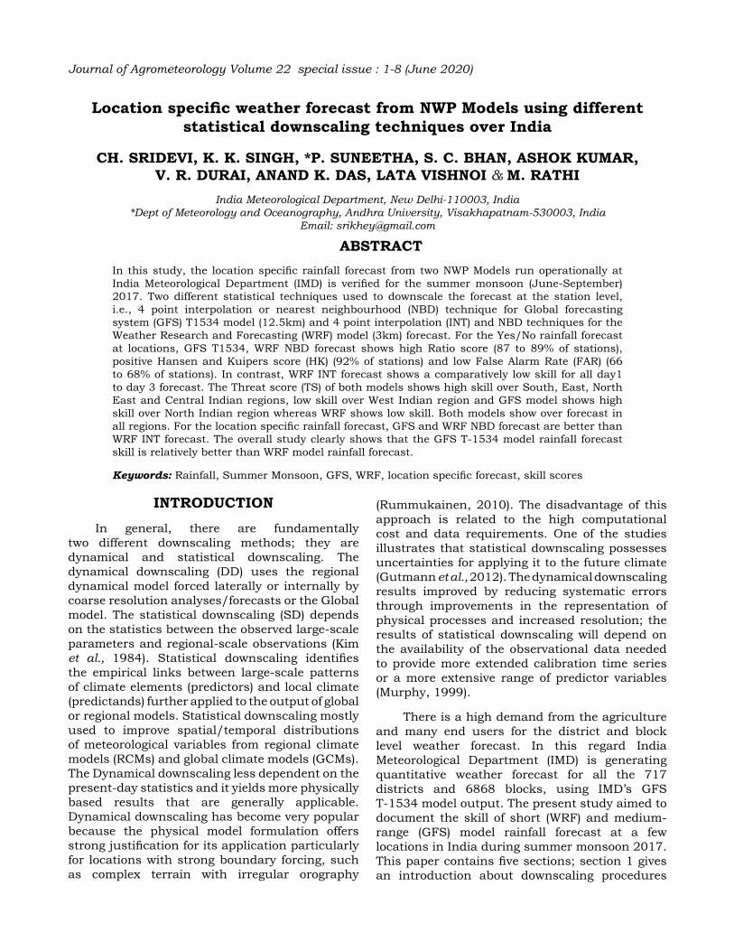
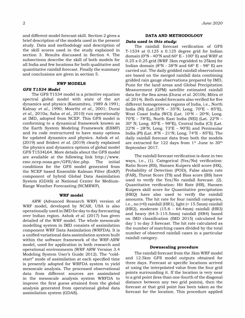
The spatial verification of yes/no rainfall forecast of GFS T1534 (12.5km) and WRF (25km) model for June to September (JJAS) 2017 has been done for the Indian window. Here only a few skill scores figures are given for brevity. The skill of both models in terms of RS (Fig. 1), shows high skill, ranges between 50-95% for all day 1 to day 3 forecast. Both models show high RS over the heavy rainfall regions of the west coast, East and North-East Indian regions. In the rain shadow regions of southern India, the GFS show high skill compare to WRF. The HKQ score for four merged rainfall thresholds of both models shows positive skill (>0) over most parts of India. As comparing to GFS model, WRF model shows negative skill over few parts of heavy rainfall regions of the west coast, northeast and eastern parts of India. The categorical and quantitative rainfall forecast skill for the five homogeneous regions of India is shown in Fig. 2. The yes/no rainfall forecast verification shows high RS score of 60 to 78%, with overall high RS (>70%) over NEI. The quantitative rainfall forecast of both models shows high HR of 0.4 to 0.56 overall the regions for all day 1 to day 3 forecast. However, both model forecast shows high HR (>0.5) over North India.

Fig. 1: Spatial distribution of Ratio score of GFS (upper panel) and WRF (lower panel) model day 1, day 2 & day 3 rainfall forecast during JJAS-2017.

Fig. 2: Skill scores (RS, HK, HR and HKQ) of GFS T1534 and WRF day 3 rainfall forecast during summer monsoon (JJAS) 2017 over 5 homogeneous regions along with all India.

Vol. 22, Special Issue SRIDEVI et al. 3

4 June 2020

In overall spatial verification, results show that the skill of the GFS model is high for all day 1 to day 3, but WRF model skill decreases from day 2 onwards. The verification of homogeneous regions also shows that GFS model skill is relatively better than the WRF model for all day1 to day 3 forecast.

Location-specific rainfall forecast skill:

Fig. 3: Spatial representation of HK score for day1 (upper) & day3 (lower) location specific weather forecast from GFS T1534 (12.5km), WRF (3km) INT and WRF (3km) NBD during JJAS 2017.

Fig. 4: Spatial representation of POD score of day 1 (upper), day 3 (lower) location specific weather forecast from GFS T1534 (12.5km), WRF (3km) INT and WRF (3km) NBD during JJAS 2017.

The main objective of the current study is to analyze the location specific rainfall forecast skill of two high resolution models using INT and NBD techniques. The models skill has been assessed by computing the Ratio Score, HK (Fig. 3), POD (Fig. 4), FAR, TS (Fig. 5) and BIAS (Fig. 6) score for yes/no rainfall and Hit Rate & HKQ calculated for different threshold rainfall amounts. The hit rate for four rainfall categories (HR1, HR2, HR3 and HR4) also calculated. The results of both models are as follows:

Fig. 5: Threat score for day1 location specific weather forecast from GFS T1534 (12.5km), WRF (3km) INT and WRF (3km) NBD over six homogeneous regions during JJAS 2017.

Fig. 6: Bias score for day1 (upper) location specific weather forecast from GFS T1534 (12.5km), WRF (3km) Interpolated (INT) and WRF (3km) nearest neighbourhood (NBD) over six (SI, NI, WI, EI, NEI & CI) homogeneous regions during JJAS 2017.

Yes/No Rainfall forecast:The Ratio Score measures the percentage of

correct forecasts out of the total forecasts issued. RS heavily influenced by most common category, usually “no events” in case of unusual weather. If

the RS is 100%, then the forecast is perfect and is less than 50%, then the forecast is weak. The highest RS score is 95% for both models.

It is observed that around 80 to 90% of stations show high RS (RS>50%) for GFS and WRF models forecast. However, WRF NBD shows relatively better skill over more locations as compared to GFS and WRF INT in all day 1, day 2 and day 3 forecast. If HK & HKQ scores are closer to 1, the forecasts are best, and when the score is near or less than 0, then the forecasts are false (Kumar et al. 2000; Bhardwaj et al. 2009). The highest value of HK score is 0.7 for both models. GFS shows positive skill over 92, 89, 80% of stations, whereas WRF INT forecast shows positive skill over 88, 87, 82% of stations and WRF NBD forecast shows positive skill over 92, 88, 86% of stations for day 1, day 2 and day 3 forecasts (Fig. 3) respectively. For the HK score, GFS and WRF NBD forecast show positive skill over maximum locations compared to WRF INT forecast. GFS model shows high skill (POD>0.5) over 98% of stations. WRF INT forecast shows high skill over 99% of stations and WRF NBD forecast shows high skill over 98, 96, 94% of stations for all day 1, day 2 and day 3 (Fig. 4) respectively. Both the models show high POD score. GFS model shows high skill (FAR<0.5) over 66, 64, 61% of stations. The WRF INT forecast shows high skill over 64, 61, 61% of stations and WRF NBD shows high skill over 68, 67, 65% of stations for all day 1, day 2 and day 3 respectively. For FAR also GFS and WRF NBD forecast shows high skill compared to WRF INT forecast.

The Threat scores (TS) also called a critical success index (CSI) measures the fraction of observed/forecast events that correctly predicted. Fig. 5 shows the TS for locations of six different regions of India. Over SI region, high (TS>0.5) skill observed over 48 to 53% of stations in both models and NI region also shows high skill over 45 to 29% of stations in both models for all day 1 to day 3 forecasts. Here the GFS model forecast shows high skill compared to WRF INT & WRF NBD forecast. Over East India region, high skill observed over 94% of stations in both models day 1 forecast. However, from day 2 onwards, 50% of stations show high skill in both models day 2 and day 3 forecasts. Over East India, WRF INT forecast shows high skill compared to GFS & WRF NBD forecasts. The NEI also shows high skill over maximum (81 to 75%) stations in both models for all day 1 to day 3 forecasts. Over NEI also GFS

model shows high skill compared to WRF INT & WRF NBD forecast. Both models show high skill over 23 - 39% of stations over WI for all day 1 to day 3 forecasts. The GFS model shows high skill over WI, compared to WRF INT & WRF NBD forecast. Over CI region high skill observed over 66 to 59% of stations in both models for all day1 to day 3 forecast. Similarly, over CI, also GFS model shows high skill compared to WRF INT & WRF NBD forecast. In overall GFS model shows high TS over maximum locations compared to WRF INT & NBD forecast.

The model frequency bias (BIAS) as shown in Fig. 6 measures the ratio of the frequency of forecast events to the frequency of observed events. BIAS indicates whether the forecast system tends to under forecast (BIAS<1), over forecast (BIAS>1) or correctly forecast (BIAS=1) events. It does not, however, measure how well the forecast corresponds to the observations but only measures relative frequencies (Durai et al., 2010b). The BIAS score over South India is as follows, the correct forecast observed over 25, 47, 23% of stations in GFS; 20, 43, 29% of stations in WRF INT forecast and 24, 44, 31% of stations in WRF NBD forecast for all day1 to day3 forecasts respectively. Over forecasting is observed over 72, 49, 75% of stations in GFS; 80, 49, 69% of stations in WRF INT forecast and 76, 48, 63% of stations in WRF NBD forecast for all day 1 to day 3 forecast respectively. Under forecasting is not observed over SI for all day 1 to day 3. Compared to the GFS forecast, WRF forecast using both techniques shows high over forecasting. Over North India region also both models show correct forecast over very few (14 to 20%) stations in all day 1 to day 3 forecasts. 70 to 80% of stations show over forecast for both models and under forecasting also observed over 4 to 12% of stations. Here GFS, WRF INT forecast shows high over forecasting compared to WRF NBD forecast. Under forecasting is not observed over East India for all day 1 to day 3 forecasts of both models, the correct forecast is observed over 40 to 50% of stations and remaining 40 - 50% stations shows over forecasting in day 1 forecast from both models. However, in day 2 and day 3 both models show over forecasting over maximum (85 to 95%) stations. Over North-East India also under forecasting is not observed in all day 1 to day 3 forecasts of both models, the correct forecast is observed over few (23 to 27%) stations and over forecasting is observed over maximum (71 to 77%) stations. Under forecasting


6 June 2020

is not observed over WI in both models day 1 to day 3 forecasts. For WI, also correct forecast is observed over very few (5 to 7%) stations and over forecasting is observed over maximum (95 to 91%) stations for all day 1 to day 3 forecasts of both models. Over Central India also under forecasting is very less, the correct forecast is observed over very few (11 to 20%) stations and over forecasting is observed over most (80 to 87%) stations in both models day1 to day3 forecasts.

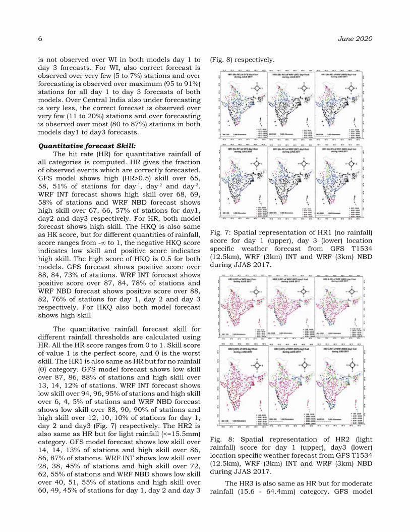
Quantitative forecast Skill:The hit rate (HR) for quantitative rainfall of

all categories is computed. HR gives the fraction of observed events which are correctly forecasted. GFS model shows high (HR>0.5) skill over 65, 58, 51% of stations for day-1, day-2 and day-3. WRF INT forecast shows high skill over 68, 69, 58% of stations and WRF NBD forecast shows high skill over 67, 66, 57% of stations for day1, day2 and day3 respectively. For HR, both model forecast shows high skill. The HKQ is also same as HK score, but for different quantities of rainfall, score ranges from -∞ to 1, the negative HKQ score indicates low skill and positive score indicates high skill. The high score of HKQ is 0.5 for both models. GFS forecast shows positive score over 88, 84, 73% of stations. WRF INT forecast shows positive score over 87, 84, 78% of stations and WRF NBD forecast shows positive score over 88, 82, 76% of stations for day 1, day 2 and day 3 respectively. For HKQ also both model forecast shows high skill.

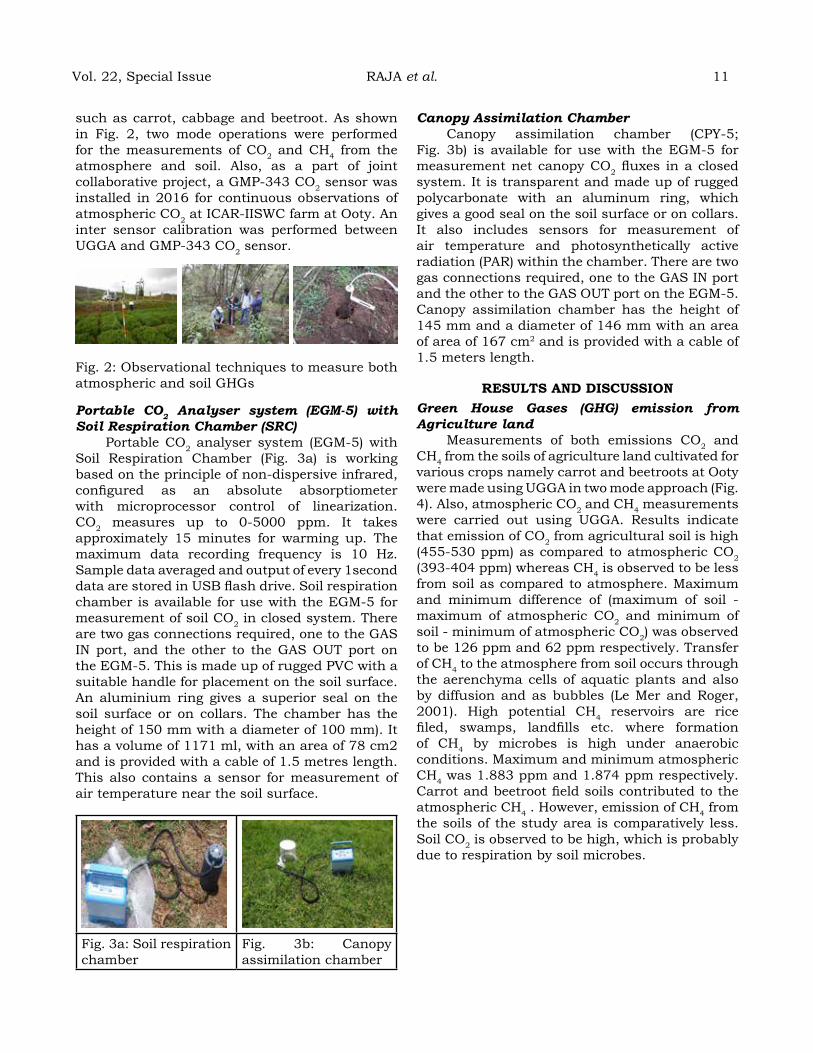
The quantitative rainfall forecast skill for different rainfall thresholds are calculated using HR. All the HR score ranges from 0 to 1. Skill score of value 1 is the perfect score, and 0 is the worst skill. The HR1 is also same as HR but for no rainfall (0) category. GFS model forecast shows low skill over 87, 86, 88% of stations and high skill over 13, 14, 12% of stations. WRF INT forecast shows low skill over 94, 96, 95% of stations and high skill over 6, 4, 5% of stations and WRF NBD forecast shows low skill over 88, 90, 90% of stations and high skill over 12, 10, 10% of stations for day 1, day 2 and day3 (Fig. 7) respectively. The HR2 is also same as HR but for light rainfall (<=15.5mm) category. GFS model forecast shows low skill over 14, 14, 13% of stations and high skill over 86, 86, 87% of stations. WRF INT shows low skill over 28, 38, 45% of stations and high skill over 72, 62, 55% of stations and WRF NBD shows low skill over 40, 51, 55% of stations and high skill over 60, 49, 45% of stations for day 1, day 2 and day 3

(Fig. 8) respectively.

Fig. 7: Spatial representation of HR1 (no rainfall) score for day 1 (upper), day 3 (lower) location specific weather forecast from GFS T1534 (12.5km), WRF (3km) INT and WRF (3km) NBD during JJAS 2017.

Fig. 8: Spatial representation of HR2 (light rainfall) score for day 1 (upper), day3 (lower) location specific weather forecast from GFS T1534 (12.5km), WRF (3km) INT and WRF (3km) NBD during JJAS 2017.

The HR3 is also same as HR but for moderate rainfall (15.6 - 64.4mm) category. GFS model

forecast shows low skill over 86, 90, 88% of stations and high skill over 14, 10, 12% of stations. WRF INT forecast shows low skill over 87, 90, 95% of stations and high skill over 13, 10, 5% of stations and WRF NBD shows low skill over 87, 91, 94% of stations and high skill over 13, 9, 6% of stations for day1, day2 and day3 (Fig. 9) respectively. The HR4 is also same as HR but for heavy rainfall (64.5-115.5mm) category. GFS model forecast shows low skill over 76, 87, 73% of stations and high skill over 24, 13, 27% of stations. WRF INT forecast shows low skill over 83, 87, 91% of stations and high skill over 17, 13, 9% of stations and WRF NBD forecast shows low skill over 81, 84, 91% of stations and high skill over 19, 16, 9% of stations for day 1, day 2 and day 3 (Fig. 9) respectively.

Fig. 9. Spatial representation of HR3 (moderate rainfall) score for day 1 (upper), day 3 (lower) location specific weather forecast from GFS T1534 (12.5km), WRF (3km) INT and WRF (3km) NBD during JJAS 2017.

SuMMarY aNd CoNCLuSIoNS:For the location-specific yes/no rainfall, GFS

T-1534 & WRF NBD forecast shows high skill

scores of Ratio score (87 to 89% of stations), HK (92% of stations) and FAR (66 to 68% of stations) whereas WRF INT forecast shows a comparatively low skill for all day 1 to day 3 forecast. POD scores of both models are high (98 to 99% of stations) and comparable for all the three days. For quantitative rainfall forecast, overall hit rate (HR) and HKQ of both models show high skill (65 to 88% of stations) for all day 1 to day 3. The Threat score of both models shows high skill (48 to 53 % of stations) over SI region. The GFS model shows high skill (45-39% of stations) and the WRF model shows low skill (39 to 37 % of stations) over the NI region. Both models show very high skill over 94 - 100% stations in day1 and 50 - 60% of stations in day2 and day3 over EI region. Both models show high skill over 75 - 81% of stations over NEI and 59 - 70% of stations over central India. However both the models show very low skill over maximum locations (59 to 75% of stations) of west India region for all day 1 to day 3 forecast. In terms of model bias in forecasting rainfall frequency, both models show over forecasting in all regions for day 1 to day 3. The over forecasting is high over West India particularly for all day1 to day3WRF forecast.

In case of different rainfall thresholds, both models show low skill over most of the locations for forecasting no rainfall (HR1), However, WRF INT shows relatively better skill than GFS and WRF NBD forecast. GFS model shows high skill (86% of stations) comparing to WRF INT (60% of stations) & WRF NBD (72% of stations) HR for light rainfall (HR2) forecast. The moderate rainfall (HR3) forecast skill of both models is very low (25-33%). For the heavy rainfall (HR4) also the skill is very less, however GFS model shows relatively better skill than both WRF INT & WRF NBD. In overall hit rate for different categories of rainfall (HR1, HR2, HR3 and HR4) are mostly better for T-1534 model. From both the model comparisons, it is clear that the GFS T1534 model rainfall forecast is relatively better than WRF model rainfall forecast.

aCKNoWLedgeMeNtSAuthors are thankful to Director General of

Meteorology, India Meteorological Department for all support and suggestions to complete this research work. Authors also like to thank NWP division IMD for making model and observational data available. Authors acknowledge the availability of GFS T1534 model forecast data


8 June 2020

from IITM, Pune.

reFereNCeSAshok Kumar, Nabansu Chattopadhayay, Y. V.

Ramarao, K. K. Singh, V. R. Durai, Ananda K. Das, Mahesh Rathi, Pradeep Mishra, K. Malathi, Anil Soni And Sridevi. (2017). Block level weather forecast using direct model output from NWP models during monsoon season in India. Mausam, Vol. 68 (1) : 23-40.

Bhardwaj R., Ashok Kumar and Parvinder Maini. (2009). ‘Statistical interpretation forecast and its skill during monsoon season in India’. International Journal of Meteorology, 34 (336), pp 39-47

Durai V.R., Roy Bhowmik S.K.R. and Mukhopadhaya B. (2010a). Performance Evaluation of Precipitation Prediction skill of NCEP Global Forecasting System (GFS) over Indian region during summer Monsoon 2008. Mausam, 61 (2) :139-154.

Durai V.R., Bhowmik S.K.R. and Mukhopadhaya. B. (2010b). Evaluation of Indian summer monsoon rainfall features using TRMM and KALPANA-1 satellite derived precipitation and rain gauge observation. Mausam, 61 (3) :317-336

Gutmann E.D, R.M. Rasmussen, C. Liu, K. Ikeda, D.J. Gochis, M.P. Clark, J. Dudhia and G. Thompson. (2012). A comparison of statistical and dynamical downscaling of winter precipitation over complex terrain. J. Climate, 25, 262-281. DOI: 10.1175/2011JCLI4109.1

IMD (2015) Weather Forecasting Circular No. 5/2015 (3.7)

Kalnay, M. Kanamitsu, and W.E. Baker. (1990). Global numerical weather prediction at the National Meteorological Center. Bull. Amer. Meteor. Soc., 71, 1410-1428.

Kanamitsu M. (1989). Description of the NMC global data assimilation and forecast system. Weather and Forecasting, 4, 335-342.

Kanamitsu M., J.C. Alpert, K.A. Campana, P.M. Caplan, D.G. Deaven, M. Iredell, B. Katz,

H.L. Pan, J. Sela and G.H. White. (1991). Recent changes implemented into the global forecast system at NMC. Weather and Forecasting, 6, 425-435.

Kim J.W., J.T. Chang, N.L. Baker, D.S. Wilks and W.L. Gates. (1984). The statistical problem of climate inversion: Determination of the relationship between local and large-scale climate. Mon. Wea. Rev., 112, 2069-2077.

Kumar A., Parvinder Maini, Rathore L.S. and S.V. Singh. (2000). An operational medium range local weather forecasting system developed in India. Int. J. Climatol., 20: 73- 87.

Kumar, A., Sridevi, C., Durai, V.R. et al. (2019). MOS guidance using neural network for the rainfall forecast over India. J Earth Syst Sci., 128:130. https://doi.org/10.1007/s12040-019-1149-y.

Mitra A.K., Satya Prakash, Imranali M. Momin, D.S. Pai and A.K. Srivastava. (2014). Daily Merged Satellite Gauge Real-Time Rainfall Dataset for Indian Region; Vayumandal, 40 (1-4).

Moorthi S., H.L. Pan. and P. Caplan. (2001). Changes to the 2001 NCEP operational MRF/AVN global Analysis/forecast system. NWS Technical Procedures Bulletin, 484, pp14. Available at http://www.nws.noaa.gov/om/tpb/484.htm.

Murphy J. (1999). An evaluation of statistical and dynamical techniques for downscaling local climate. J. Climate, 12, 2256-2284.

Murphy A.H. and Katz R.W. (1985). Probability, Statistics and decision making in the Atmospheric Sciences. Westview Press, 545 pp.

Rummukainen M. (2010). State-of-the-art with regional climate models. WIREs Clim. Change., 1, 82-96.

Saha, Suranjana, and Coauthors. (2010). The NCEP Climate Forecast System Reanalysis. Bull. Amer. Meteor. Soc., 91, 1015–1057.

Sridevi C., Singh K.K., Suneetha P., Durai V.R. and Kumar A. (2019). Rainfall forecasting skill of GFS model at T1534 and T574 resolution over India during monsoon season. Meteorol Atmos Phys., https://doi.org/10.1007/s00703-019-00672-x.

Study on Co2 and Ch4 emissions from the soils of various land use systems in temperate mountainous ecosystem of part of Nilgiris,

Western ghats, India

P. raJa1* K.raJaN1, P.MaheSh2, K.KaNNaN1, u.SureNdraN3, K.MaLLIKarJuN2 o.P.S KhoLa1 aNd C.aruLMathI1

1ICAR-Indian Institute of Soil and Water Conservation, Research Centre, Udhagamandalam- 643004, The Nilgiris, Tamil Nadu.

2ISRO-National Remote Sensing Centre, Climate Studies Group-ECSA, Hyderabad-5000373Centre for Water Resources Development and Management, Calicut, Kerala

*Corresponding Author E-mail: [email protected]

aBStraCtHigh altitude ecosystems are highly vulnerable and are generally subjected to rapid changes of climate especially due to change in land use practices and deforestation. It affects the emission level of Green House Gases (GHGs) particularly carbon dioxides (CO2). Forest soil possess huge quantity of mineralizable soil organic carbon (SOC), with high microbial communities and soil respiration. However frequent land use change strongly influences the quality and quantity of SOC, since it is largely governed by the microbial population and soil respiration. Therefore, the present study is taken up to find out CO2 and CH4 emissions from the soils of forest, grassland, tea plantations and agricultural land. We found that the soils of grassland emits maximum amount of greenhouse gases and the soils of the agricultural land, emits minimum amount of GHG’s. However, the grassland and forest soils along with the vegetation cover behave as a sink to the atmospheric CO2. We conclude that the protection of forests and grasslands is essential to prevent top soil erosion, sustenance in soil quality and for amelioration of global warming effects.

Keywords: Atmospheric CO2, Grassland, Green House Gases (GHGs), Shola, Western Ghats

INtroduCtIoN

Green House Gases (GHG) such as CO2, CH4 are significant in regulating the climate of lower atmosphere (IPCC-AR5, 2015). It is hence very important to monitor spatial and temporal variations of these gases in order to address their climate forcing and impact on biosphere (WMO, 2009). The average concentration of carbon dioxide was 390.5 ppm in 2011, which is an increase of 40 per cent from the year 1750. Atmospheric methane (CH4) was at 1803.2 ppb (1801.2 to 1805.2) in 2011; this is 150 per cent greater than the level before the year 1750 (Hartmann et al., 2013). Carbon dioxide and Methane which together contribute to 80 per cent of total anthropogenic radiative forcing, leading to global warming (Forster et al., 2007; Kobayashi et al., 2010). Battle et al., (2000) reported based on previous studies with the available surface in-situ network observations that the oceans and biosphere absorbs more than 50 percent of CO2 emissions. While these measurements of CO2 are accurate up to 0.1 ppm, it remains doubtful to predict the response to the climate changes in future due to wider geographic distribution and the nature of these sinks (Yang et al., 2008;

Deutscher et al., 2010). Precise global columnar concentrations of GHGs measurements are essential to investigate the spatial variations of CO2 emissions across the Globe.

Alarming increase in the levels of Green House Gases (GHGs) and carbon dioxide (CO2) due to global warming are now recognized as a serious threat to environmental systems.. Currently the land use systems are considered as a potential mean for sequestering more C as sink and many researchers are working on the measurement of C sink (Mohan Kumar and Nair, 2011). In order to understand the response of different land use systems on atmospheric CO2, a collaborative research activity was initiated between ICAR-Indian Institute of Soil and Water Conservation Udhagamandalam and ISRO-National Remote Sensing Service Centre, Hyderabad.

As part of this collaborative study, a field campaign was conducted in August 2017 to carry out measurements of CO2, CH4 and H2O from different land use systems viz., forests, grassland, tea plantation and agricultural land from parts of Nilgiris in Western Ghats around Udhagamandalam. By keeping these points, we


10 June 2020

aimed to study the exchange of GHGs between soil-land use systems and atmosphere and soil in part of Nilgiris, Western Ghats, India.

MaterIaLS aNd MethodSStudy Area

The study area of Udhagamandalam is in temperate ecosystem of the Nilgiris in Tamil Nadu. The average maximum and mean minimum temperature is 19.8°C and 11°C, respectively. The month of April was the hottest with average maximum temperature of 23.3°C and January was the coolest with mean minimum temperature of 6.4°C. So far the maximum temperature recorded in Udhagamandalam was 25°C and the lowest temperature was −2 °C. Annual precipitation is 1250 mm with a marked drier season from December to March. Elevation of the study area ranges from 2000 to 2250 m MSL. Major land uses in the study area are various type of forests (natural forest, pine, mixed, eucalyptus), grasslands, tea plantation and agriculture (vegetable cultivations). Soils of the study area are mainly red and lateritic and of acidic in nature. Measurements were taken in forests predominantly of eucalyptus with a land slope of 10-12 per cent with thin layer of litters. Tea with dense cover of the crop with land slope of 10-12 per cent. The age of tea crop is 30 years. Vegetable crops of carrot and beet root were grown in nearly flat land. Forest, grassland, tea and agriculture soils have varied levels of carbon content due to nature of its vegetation and it influences the CO2 emission as well. Hence, the measurement of CO2, CH4 was done using Ultraportable Greenhouse Gas Analyzer (UGGA) and measurement of soil and plant CO2 using soil respiration and canopy assimilation chamber respectively.

Technical details of Ultraportable Greenhouse Gas Analyzer

Ultraportable Greenhouse Gas Analyzer (UGGA 915-LGR – GLA 132), (Fig. 1) measures methane, carbon dioxide and water vapour simultaneously using a single analyser. The working principle involves using an analyzer, which utilizes a unique laser absorption technology called Off-Axis Integrated Cavity Output Spectroscopy (OA-ICOS). There are two lasers used in this measurement. Laser with 1.6 micron for CO2 measurement and with 1.65 micron for CH4 measurement. We can manually fix the inlets for the simultaneous measurement of soil emission of CO2 and CH4. Similarly we can

simultaneously measure atmospheric CO2 and CH4. However, simultaneous measurements of both soil and atmospheric CO2 and CH4 cannot be carried out as the analyser has only one input. The maximum data recording frequency is 10 Hz. The pump has a nominal flow rate of 0.5 l/min. UGGA reports and stores all measured fully resolved absorption spectra which allows the instrument to accurately correct for water vapour dilution and absorption line broadening effects and thus to report CH4 and CO2 on a dry (and wet) mole fraction basis directly without drying or post processing.

Fig. 1: Ultraportable Greenhouse Gas Analyzer (UGGA 915)

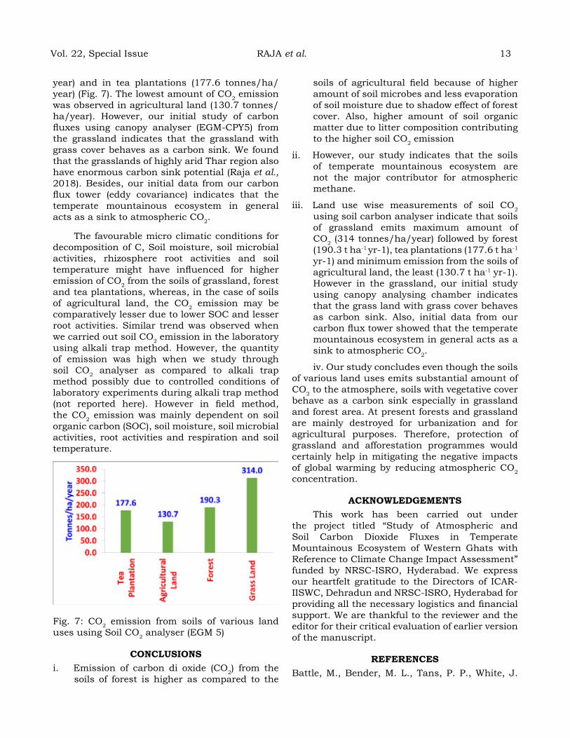
Fig. 2: Observational techniques to measure both atmospheric and soil GHGs

Using high precision UGGA, observations on CO2, and CH4 were carried out over Agriculture area (Carrot and Beetroot cultivation), un-disturbed forest of Eucalyptus and Tea plantation respectively. By using EGM-5 soil CO2 measuring portable system, soil CO2 emission was measured in grasslands, forest, tea plantation and agricultural land cultivated mainly for vegetable

such as carrot, cabbage and beetroot. As shown in Fig. 2, two mode operations were performed for the measurements of CO2 and CH4 from the atmosphere and soil. Also, as a part of joint collaborative project, a GMP-343 CO2 sensor was installed in 2016 for continuous observations of atmospheric CO2 at ICAR-IISWC farm at Ooty. An inter sensor calibration was performed between UGGA and GMP-343 CO2 sensor.

Fig. 2: Observational techniques to measure both atmospheric and soil GHGs

Portable CO2 Analyser system (EGM-5) with Soil Respiration Chamber (SRC)

Portable CO2 analyser system (EGM-5) with Soil Respiration Chamber (Fig. 3a) is working based on the principle of non-dispersive infrared, configured as an absolute absorptiometer with microprocessor control of linearization. CO2 measures up to 0-5000 ppm. It takes approximately 15 minutes for warming up. The maximum data recording frequency is 10 Hz. Sample data averaged and output of every 1second data are stored in USB flash drive. Soil respiration chamber is available for use with the EGM-5 for measurement of soil CO2 in closed system. There are two gas connections required, one to the GAS IN port, and the other to the GAS OUT port on the EGM-5. This is made up of rugged PVC with a suitable handle for placement on the soil surface. An aluminium ring gives a superior seal on the soil surface or on collars. The chamber has the height of 150 mm with a diameter of 100 mm). It has a volume of 1171 ml, with an area of 78 cm2 and is provided with a cable of 1.5 metres length. This also contains a sensor for measurement of air temperature near the soil surface.

Fig. 3a: Soil respiration chamber

Fig. 3b: Canopy assimilation chamber

Canopy Assimilation ChamberCanopy assimilation chamber (CPY-5;

Fig. 3b) is available for use with the EGM-5 for measurement net canopy CO2 fluxes in a closed system. It is transparent and made up of rugged polycarbonate with an aluminum ring, which gives a good seal on the soil surface or on collars. It also includes sensors for measurement of air temperature and photosynthetically active radiation (PAR) within the chamber. There are two gas connections required, one to the GAS IN port and the other to the GAS OUT port on the EGM-5. Canopy assimilation chamber has the height of 145 mm and a diameter of 146 mm with an area of area of 167 cm2 and is provided with a cable of 1.5 meters length.

reSuLtS aNd dISCuSSIoNGreen House Gases (GHG) emission from Agriculture land

Measurements of both emissions CO2 and CH4 from the soils of agriculture land cultivated for various crops namely carrot and beetroots at Ooty were made using UGGA in two mode approach (Fig. 4). Also, atmospheric CO2 and CH4 measurements were carried out using UGGA. Results indicate that emission of CO2 from agricultural soil is high (455-530 ppm) as compared to atmospheric CO2 (393-404 ppm) whereas CH4 is observed to be less from soil as compared to atmosphere. Maximum and minimum difference of (maximum of soil - maximum of atmospheric CO2 and minimum of soil - minimum of atmospheric CO2) was observed to be 126 ppm and 62 ppm respectively. Transfer of CH4 to the atmosphere from soil occurs through the aerenchyma cells of aquatic plants and also by diffusion and as bubbles (Le Mer and Roger, 2001). High potential CH4 reservoirs are rice filed, swamps, landfills etc. where formation of CH4 by microbes is high under anaerobic conditions. Maximum and minimum atmospheric CH4 was 1.883 ppm and 1.874 ppm respectively. Carrot and beetroot field soils contributed to the atmospheric CH4 . However, emission of CH4 from the soils of the study area is comparatively less. Soil CO2 is observed to be high, which is probably due to respiration by soil microbes.

Vol. 22, Special Issue RAJA et al. 11

12 June 2020

Fig. 4a: Carrot Field

4b. Beet root Field

GHGs over Eucalyptus undisturbed forestMinimum and maximum CO2 emission from

soil of eucalyptus forest was 595 ppm and 685 ppm respectively. Minimum and maximum and level of atmospheric CO2 was observed as 402 ppm and 418 ppm respectively. Minimum and maximum CH4 level in atmosphere was observed as 1.882 and 1.900 ppm. Likewise minimum and maximum soil CH4 emission was measured as 1.878 ppm and 1.902 ppm respectively. The present study indicates less contribution of CH4 to the atmosphere from soil under eucalyptus forest. However, soil CO2 emission in forest was observed to be high, which is probably due to respiration of microorganisms and roots present in the soils. Also, increase in soil organic carbon due to leaf decomposition and higher moisture content in soils are contributing the higher emission of

carbon di oxides from forest soils.

Fig. 5: CO2 and CH4 observations over Eucalyptus forest at Ooty

ghgs over tea PlantationIn the tea plantation area maximum and

minimum atmospheric CO2 and CH4 measured was 421; 406.2 ppm and 1.935; 1.875 ppm respectively, (Fig. 6).

Fig. 6: CO2 and CH4 observations over Tea plantation at Ooty.

CO2 emission from the soils of different land use System using Soil CO2 Analyzer- (EGM)

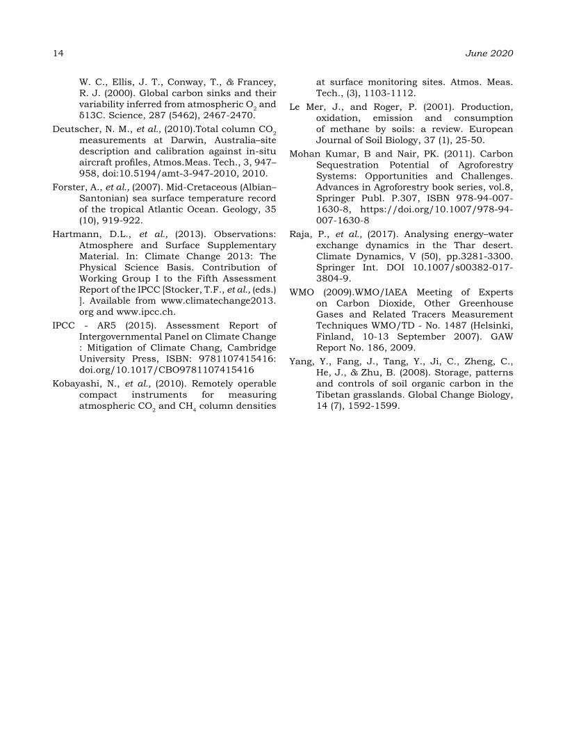
Carbon dioxide evolution was estimated in the field using portable CO2 analyser (EGM-5 of PP Systems) with canopy assimilation chamber. Our results indicate that CO2 emission was found to be more in the soils of grassland (314 tonnes/ha/year) followed by forest (190.3 tonnes/ha/

year) and in tea plantations (177.6 tonnes/ha/year) (Fig. 7). The lowest amount of CO2 emission was observed in agricultural land (130.7 tonnes/ha/year). However, our initial study of carbon fluxes using canopy analyser (EGM-CPY5) from the grassland indicates that the grassland with grass cover behaves as a carbon sink. We found that the grasslands of highly arid Thar region also have enormous carbon sink potential (Raja et al., 2018). Besides, our initial data from our carbon flux tower (eddy covariance) indicates that the temperate mountainous ecosystem in general acts as a sink to atmospheric CO2.

The favourable micro climatic conditions for decomposition of C, Soil moisture, soil microbial activities, rhizosphere root activities and soil temperature might have influenced for higher emission of CO2 from the soils of grassland, forest and tea plantations, whereas, in the case of soils of agricultural land, the CO2 emission may be comparatively lesser due to lower SOC and lesser root activities. Similar trend was observed when we carried out soil CO2 emission in the laboratory using alkali trap method. However, the quantity of emission was high when we study through soil CO2 analyser as compared to alkali trap method possibly due to controlled conditions of laboratory experiments during alkali trap method (not reported here). However in field method, the CO2 emission was mainly dependent on soil organic carbon (SOC), soil moisture, soil microbial activities, root activities and respiration and soil temperature.

Fig. 7: CO2 emission from soils of various land uses using Soil CO2 analyser (EGM 5)

CoNCLuSIoNSi. Emission of carbon di oxide (CO2) from the

soils of forest is higher as compared to the

soils of agricultural field because of higher amount of soil microbes and less evaporation of soil moisture due to shadow effect of forest cover. Also, higher amount of soil organic matter due to litter composition contributing to the higher soil CO2 emission

ii. However, our study indicates that the soils of temperate mountainous ecosystem are not the major contributor for atmospheric methane.

iii. Land use wise measurements of soil CO2 using soil carbon analyser indicate that soils of grassland emits maximum amount of CO2 (314 tonnes/ha/year) followed by forest (190.3 t ha-1 yr-1), tea plantations (177.6 t ha-1

yr-1) and minimum emission from the soils of agricultural land, the least (130.7 t ha-1 yr-1). However in the grassland, our initial study using canopy analysing chamber indicates that the grass land with grass cover behaves as carbon sink. Also, initial data from our carbon flux tower showed that the temperate mountainous ecosystem in general acts as a sink to atmospheric CO2.

iv. Our study concludes even though the soils of various land uses emits substantial amount of CO2 to the atmosphere, soils with vegetative cover behave as a carbon sink especially in grassland and forest area. At present forests and grassland are mainly destroyed for urbanization and for agricultural purposes. Therefore, protection of grassland and afforestation programmes would certainly help in mitigating the negative impacts of global warming by reducing atmospheric CO2 concentration.

aCKNoWLedgeMeNtSThis work has been carried out under

the project titled “Study of Atmospheric and Soil Carbon Dioxide Fluxes in Temperate Mountainous Ecosystem of Western Ghats with Reference to Climate Change Impact Assessment” funded by NRSC-ISRO, Hyderabad. We express our heartfelt gratitude to the Directors of ICAR-IISWC, Dehradun and NRSC-ISRO, Hyderabad for providing all the necessary logistics and financial support. We are thankful to the reviewer and the editor for their critical evaluation of earlier version of the manuscript.

reFereNCeSBattle, M., Bender, M. L., Tans, P. P., White, J.

Vol. 22, Special Issue RAJA et al. 13

14 June 2020

W. C., Ellis, J. T., Conway, T., & Francey, R. J. (2000). Global carbon sinks and their variability inferred from atmospheric O2 and δ13C. Science, 287 (5462), 2467-2470.

Deutscher, N. M., et al., (2010).Total column CO2 measurements at Darwin, Australia–site description and calibration against in-situ aircraft profiles, Atmos.Meas. Tech., 3, 947–958, doi:10.5194/amt-3-947-2010, 2010.

Forster, A., et al., (2007). Mid-Cretaceous (Albian–Santonian) sea surface temperature record of the tropical Atlantic Ocean. Geology, 35 (10), 919-922.

Hartmann, D.L., et al., (2013). Observations: Atmosphere and Surface Supplementary Material. In: Climate Change 2013: The Physical Science Basis. Contribution of Working Group I to the Fifth Assessment Report of the IPCC [Stocker, T.F., et al., (eds.) ]. Available from www.climatechange2013.org and www.ipcc.ch.

IPCC - AR5 (2015). Assessment Report of Intergovernmental Panel on Climate Change : Mitigation of Climate Chang, Cambridge University Press, ISBN: 9781107415416: doi.org/10.1017/CBO9781107415416

Kobayashi, N., et al., (2010). Remotely operable compact instruments for measuring atmospheric CO2 and CH4 column densities

at surface monitoring sites. Atmos. Meas. Tech., (3), 1103-1112.

Le Mer, J., and Roger, P. (2001). Production, oxidation, emission and consumption of methane by soils: a review. European Journal of Soil Biology, 37 (1), 25-50.

Mohan Kumar, B and Nair, PK. (2011). Carbon Sequestration Potential of Agroforestry Systems: Opportunities and Challenges. Advances in Agroforestry book series, vol.8, Springer Publ. P.307, ISBN 978-94-007-1630-8, https://doi.org/10.1007/978-94-007-1630-8

Raja, P., et al., (2017). Analysing energy–water exchange dynamics in the Thar desert. Climate Dynamics, V (50), pp.3281-3300. Springer Int. DOI 10.1007/s00382-017-3804-9.

WMO (2009).WMO/IAEA Meeting of Experts on Carbon Dioxide, Other Greenhouse Gases and Related Tracers Measurement Techniques WMO/TD - No. 1487 (Helsinki, Finland, 10-13 September 2007). GAW Report No. 186, 2009.

Yang, Y., Fang, J., Tang, Y., Ji, C., Zheng, C., He, J., & Zhu, B. (2008). Storage, patterns and controls of soil organic carbon in the Tibetan grasslands. Global Change Biology, 14 (7), 1592-1599.

analyzing uncertainties amongst the seventeen gCMs for prediction of temperature, rainfall and solar radiation in central irrigated plains in Punjab

JatINder Kaur*, PraBhJYot Kaur1 aNd SaMaNPreet Kaur2

1Department of Climate Change and Agricultural Meteorology2Department of Soil and Water Engineering

College of Agriculture, Punjab Agricultural University, Ludhiana*Corresponding author E-mail: [email protected]

aBStraCtGeneral circulation models (GCM’s) are mathematical representations of the Earth’s climate system which helps to simulate the climatic changes in the present and future time slices. In this study, daily data on meteorological parameters was downscaled from the site http://gismap.ciat.cgiar.org/MarkSimGCM/ between 2010 to 2095 time periods for Ludhiana in Punjab state. Amongst the different methods of bias removal, the “Difference method at monthly time scale” was applied on maximum temperature and rainfall data but on the daily scale for solar radiation to correct model data. There was no bias removal in minimum temperature (Tmin) because bias increased in minimum temperature if correction methods were applied. These selected models, i.e., CSIRO-Mk3-6-0, FIO-ESM, GISS-E2-R, IPSL-CM5A-MR, and one ensemble model predicted the maximum temperature to be 29.9, 29.8, 29.8, 30.3 and 29.8oC, respectively compared to the actual observed of 30.3oC; the minimum temperature to be 17.8, 17.8, 17.8, 18.0 and 17.8oC, respectively compared to the actual observed of 18.3oC; and the rainfall to be 584.7, 552.3, 557.9, 549.0 and 468.1 mm, compared to the actual observed of 546.0 mm and solar radiation 15.2, 15.2, 15.2, 15.1 and 15.2 Wm-2 compared to the actual observed of 15.3 Wm-2 respectively after bias removal.

Keywords: Bias correction, Difference method, General Circulation Models, Ludhiana, Rainfall, Solar Radiation, Temperature

INtroduCtIoN

Large-scale projections in coarse resolutions have been provided by GCM’s for various climate variables (IPCC, 2013). Still these are an important tool in generating the information on the present, past and future climate (Fowler et al., 2007) With progressive improvements as comprehension of the dynamic nature of the atmosphere has progressed (Karl and Trenberth., 2003). The GCMs have been used for various applications that simulate the advancement of climate by investigating the relationship between procedures of the atmosphere framework, simulating, and giving the projections of upcoming climate state under scenarios. The raw data from GCMs essentially needs to be corrected to arrest the influence of low frequency inconsistency of teleconnections on large-scale climatic variables. Hence the modeled output of these GCMs should preferably not be directly applied over the larger scales for the estimation of how the probable changes in climatic parameters will affect temperature and water accessibility which will ultimately influence the water supply (Dingbao Wang., 2013; Bennett et al., 2012). To counter this difficulty, efforts were made in bridging worldwide

and local climate data by developing and using a technique called “statistical downscaling”. So in many of the climate change impact studies, most commonly used techniques are dynamic and statistical downscaling in transferring climatic variables to provincial and nearby hydro-atmosphere data (Najafi and Moradkhani., 2015). The unprocessed output obtained from GCM/RCM models of the climatic parameters often has several methodical inaccuracies. These errors in the simulated precipitation and temperature on a daily basis may adversely affect the trend analysis done at daily, monthly, seasonal or annual time scale. To remove these systematic errors in the modeled data some corrections based on statistical corrective methods need to be done to make available a bias free raw data (Hansen et al., 2006; Sharma et al., 2007). Several statistical rectification methods ranging from easy to complex methods for bias removal in precipitation and temperature have been cited in literature. The basic hypothesis in these procedures are that when moving from baseline to futuristic scenario simulations, the correction methods remain stable over the time (Déqué., 2007; Hashino et al., 2007). In the statistical downscaling of the GCM’s output, the changes between observed and


16 June 2020

simulated large-scale atmospheric variables are rectified. The objectives of this research article is to enhance the reliability of future projections to be synthesized with recorded observations as inputs of the adaptive multivariate risk framework.

MaterIaLS aNd MethodSThe study was carried out for Ludhiana

(300-54’-33”N, 750-48’-22”E, 247 m above msl) located in the central irrigated plains of Punjab in Trans-Gangetic agro-climatic zones of India. The daily weather data for past years (2010–2017) on Tmax (maximum temperature), Tmin (minimum temperature), SR (solar radiation) and RF (rainfall) recorded at the agrometeorological observatory were used. Data for meteorological parameters like Tmax, Tmin, SR and RF on daily basis downscaled from General circulation models for Ludhiana station for time period of 2010–2017 were used for the calibration and validation. The GCM data were obtained from the site http://gismap.ciat.cgiar.org/MarkSimGCM/ at daily interval under RCP scenarios. The bias in the modeled data was estimated as difference between observed and modeled data at daily, monthly and annual time scales using the observed and the modeled data of 2010-2015. The bias was corrected by developing correction factors on daily and equation on monthly and annual time scales using the observed and the modeled data of 2010-2015. Their suitability was validated by applying correction factor/equation for the period 2016-17 and the statistical analysis like mean (μ), standard deviation (σ), variance (σ2), residual mean square error (RMSE) and normalized residual mean square error (NRMSE) of the maximum and minimum temperature, rainfall and solar radiation was done. The formulas were given as:

RMSE =

NRMSE=

Here Mi = modeled value

Oi = Observed value

i = Number of observations ranging from 1 to n

M = mean of observed variables

Jamieson et al., (1991) reported that the simulation is considered excellent, good, fair and poor if NRMSE is <10, 10-20, 20-30 and >30%,

respectively. When the value becomes equal to the zero for a model then it will show the best fit between observed and model data. To bring modeled data closer to the observed following method was used:

dIFFereNCe MethodIn difference method of bias removal,

daily difference between model data (Xmodel) and observed data (Xobs) of meteorological parameters (e.g. temperature, rainfall and solar radiation) for each Julian day (365 days) averaged from 6 years data (2010-15) form past records were calculated. These were taken as a “Daily Correction Factor”. Then these correction factors were subtracted from the modeled uncorrected (Xmodel uncorr) data so that the model corrected (Xmodel corr) data comes closer to the actual data. The formula for difference method of bias removal is given as under:

X (model corr) = X (model uncorr) – (Xmodel - Xobs)

Xmodel = Model data; Xmodel uncorr = Uncorrected model data; Xobs = Observed data

reSuLtS aNd dISCuSSIoNGeneral circulation model analysis

For this study, we select 4 GCM’s i.e. CSIRO-Mk3-6-0, FIO-ESM, GISS-E2-R, IPSL-CM5A-MR and one ensemble model on the basis of the statistical parameters like mean (μ), standard deviation (σ), variance (σ2), residual mean square error (RMSE) and normalized residual mean square error (NRMSE). Monthly and annual correction factors for maximum temperature, minimum temperature, rainfall, and solar radiation are given in Table 1 and Table 2. The variability in the statistical parameters like mean (μ), standard deviation (σ), variance (σ2), residual mean square error (RMSE) and normalized residual mean square error (NRMSE) of weather parameters is given in Table 3 (a, b, c and d). The four selected GCM models showed a close relationship to the observed data after bias removal which was clearly seen in Fig. 1. The results of the statistical tests of GCM’s performance to simulate historical records of climatic variables showed better simulation results for temperature and solar radiation as compared to the precipitation. Summer season like June, July and August precipitation (Beyene et al., 2010), in the catchment is affected by monsoon activity which was not precisely considered by the GCM’s (Taye et al., 2011). Bias existence was more in the precipitation data than

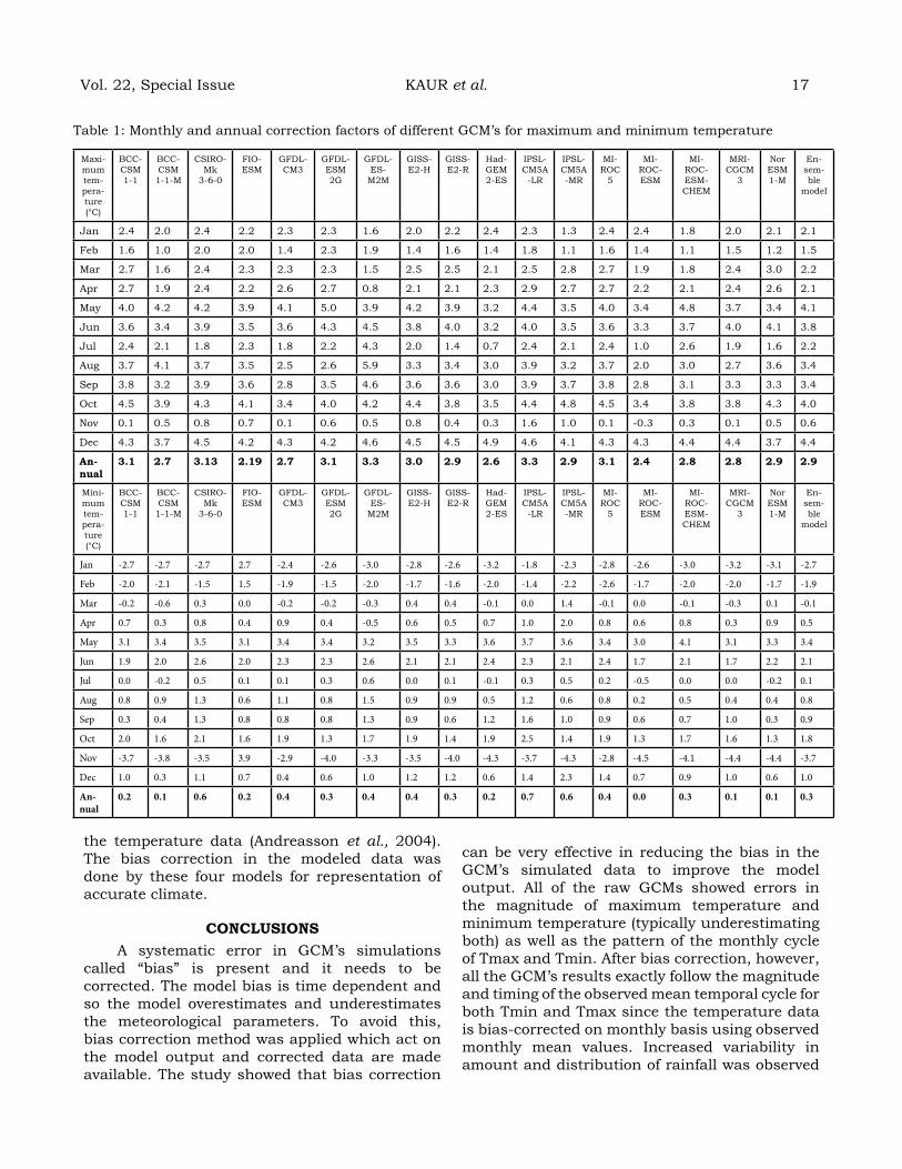
Table 1: Monthly and annual correction factors of different GCM’s for maximum and minimum temperature

Maxi-mum tem-pera-ture (°C)

BCC-CSM 1-1

BCC-CSM 1-1-M

CSIRO-Mk

3-6-0

FIO-ESM

GFDL- CM3

GFDL- ESM 2G

GFDL- ES-

M2M

GISS-E2-H

GISS-E2-R

Had-GEM 2-ES

IPSL- CM5A -LR

IPSL- CM5A -MR

MI-ROC

5

MI-ROC- ESM

MI-ROC- ESM- CHEM

MRI- CGCM

3

Nor ESM 1-M

En-sem-ble

model

Jan 2.4 2.0 2.4 2.2 2.3 2.3 1.6 2.0 2.2 2.4 2.3 1.3 2.4 2.4 1.8 2.0 2.1 2.1

Feb 1.6 1.0 2.0 2.0 1.4 2.3 1.9 1.4 1.6 1.4 1.8 1.1 1.6 1.4 1.1 1.5 1.2 1.5

Mar 2.7 1.6 2.4 2.3 2.3 2.3 1.5 2.5 2.5 2.1 2.5 2.8 2.7 1.9 1.8 2.4 3.0 2.2

Apr 2.7 1.9 2.4 2.2 2.6 2.7 0.8 2.1 2.1 2.3 2.9 2.7 2.7 2.2 2.1 2.4 2.6 2.1

May 4.0 4.2 4.2 3.9 4.1 5.0 3.9 4.2 3.9 3.2 4.4 3.5 4.0 3.4 4.8 3.7 3.4 4.1

Jun 3.6 3.4 3.9 3.5 3.6 4.3 4.5 3.8 4.0 3.2 4.0 3.5 3.6 3.3 3.7 4.0 4.1 3.8

Jul 2.4 2.1 1.8 2.3 1.8 2.2 4.3 2.0 1.4 0.7 2.4 2.1 2.4 1.0 2.6 1.9 1.6 2.2

Aug 3.7 4.1 3.7 3.5 2.5 2.6 5.9 3.3 3.4 3.0 3.9 3.2 3.7 2.0 3.0 2.7 3.6 3.4

Sep 3.8 3.2 3.9 3.6 2.8 3.5 4.6 3.6 3.6 3.0 3.9 3.7 3.8 2.8 3.1 3.3 3.3 3.4

Oct 4.5 3.9 4.3 4.1 3.4 4.0 4.2 4.4 3.8 3.5 4.4 4.8 4.5 3.4 3.8 3.8 4.3 4.0

Nov 0.1 0.5 0.8 0.7 0.1 0.6 0.5 0.8 0.4 0.3 1.6 1.0 0.1 -0.3 0.3 0.1 0.5 0.6

Dec 4.3 3.7 4.5 4.2 4.3 4.2 4.6 4.5 4.5 4.9 4.6 4.1 4.3 4.3 4.4 4.4 3.7 4.4

an-nual

3.1 2.7 3.13 2.19 2.7 3.1 3.3 3.0 2.9 2.6 3.3 2.9 3.1 2.4 2.8 2.8 2.9 2.9

Mini-mum tem-pera-ture (°C)

BCC-CSM 1-1

BCC-CSM 1-1-M

CSIRO-Mk

3-6-0

FIO-ESM

GFDL- CM3

GFDL- ESM 2G

GFDL- ES-

M2M

GISS-E2-H

GISS-E2-R

Had-GEM 2-ES

IPSL- CM5A -LR

IPSL- CM5A -MR

MI-ROC

5

MI-ROC- ESM

MI-ROC- ESM- CHEM

MRI- CGCM

3

Nor ESM 1-M

En-sem-ble

model

Jan -2.7 -2.7 -2.7 2.7 -2.4 -2.6 -3.0 -2.8 -2.6 -3.2 -1.8 -2.3 -2.8 -2.6 -3.0 -3.2 -3.1 -2.7

Feb -2.0 -2.1 -1.5 1.5 -1.9 -1.5 -2.0 -1.7 -1.6 -2.0 -1.4 -2.2 -2.6 -1.7 -2.0 -2.0 -1.7 -1.9

Mar -0.2 -0.6 0.3 0.0 -0.2 -0.2 -0.3 0.4 0.4 -0.1 0.0 1.4 -0.1 0.0 -0.1 -0.3 0.1 -0.1

Apr 0.7 0.3 0.8 0.4 0.9 0.4 -0.5 0.6 0.5 0.7 1.0 2.0 0.8 0.6 0.8 0.3 0.9 0.5

May 3.1 3.4 3.5 3.1 3.4 3.4 3.2 3.5 3.3 3.6 3.7 3.6 3.4 3.0 4.1 3.1 3.3 3.4

Jun 1.9 2.0 2.6 2.0 2.3 2.3 2.6 2.1 2.1 2.4 2.3 2.1 2.4 1.7 2.1 1.7 2.2 2.1

Jul 0.0 -0.2 0.5 0.1 0.1 0.3 0.6 0.0 0.1 -0.1 0.3 0.5 0.2 -0.5 0.0 0.0 -0.2 0.1

Aug 0.8 0.9 1.3 0.6 1.1 0.8 1.5 0.9 0.9 0.5 1.2 0.6 0.8 0.2 0.5 0.4 0.4 0.8

Sep 0.3 0.4 1.3 0.8 0.8 0.8 1.3 0.9 0.6 1.2 1.6 1.0 0.9 0.6 0.7 1.0 0.3 0.9

Oct 2.0 1.6 2.1 1.6 1.9 1.3 1.7 1.9 1.4 1.9 2.5 1.4 1.9 1.3 1.7 1.6 1.3 1.8

Nov -3.7 -3.8 -3.5 3.9 -2.9 -4.0 -3.3 -3.5 -4.0 -4.3 -3.7 -4.3 -2.8 -4.5 -4.1 -4.4 -4.4 -3.7

Dec 1.0 0.3 1.1 0.7 0.4 0.6 1.0 1.2 1.2 0.6 1.4 2.3 1.4 0.7 0.9 1.0 0.6 1.0

An-nual

0.2 0.1 0.6 0.2 0.4 0.3 0.4 0.4 0.3 0.2 0.7 0.6 0.4 0.0 0.3 0.1 0.1 0.3

the temperature data (Andreasson et al., 2004). The bias correction in the modeled data was done by these four models for representation of accurate climate.

CoNCLuSIoNSA systematic error in GCM’s simulations

called “bias” is present and it needs to be corrected. The model bias is time dependent and so the model overestimates and underestimates the meteorological parameters. To avoid this, bias correction method was applied which act on the model output and corrected data are made available. The study showed that bias correction

can be very effective in reducing the bias in the GCM’s simulated data to improve the model output. All of the raw GCMs showed errors in the magnitude of maximum temperature and minimum temperature (typically underestimating both) as well as the pattern of the monthly cycle of Tmax and Tmin. After bias correction, however, all the GCM’s results exactly follow the magnitude and timing of the observed mean temporal cycle for both Tmin and Tmax since the temperature data is bias-corrected on monthly basis using observed monthly mean values. Increased variability in amount and distribution of rainfall was observed

Vol. 22, Special Issue KAUR et al. 17

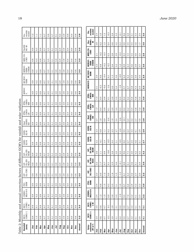
18 June 2020Ta

ble

2: M

onth

ly a

nd

ann

ual

cor

rect

ion

fact

ors

of d

iffer

ent

GC

M’s

for

rain

fall

and

sola

r ra

diat

ion

rai

nfal

l (m

m)

BC

C-

CS

M1-

1B

CC

-C

SM

1-1-

M

CS

IRO

-M

k3-6

-0FI

O-

ES

MG

F-D

L-C

M3

GF-

DL-

ES

-M

2G

GF-

DL-

ES

-M

2M

GIS

S-

E2-

HG

ISS

- E

2-R

Had

G

EM

2-E

S

IPS

L-C

M5A

-LR

IPS

L-C

M5A

-M

R

MIR

OC

5

MI

RO

C-

ES

MM

IRO

C-

ES

M-

CH

EM

MR

I-C

G-

CM

3N

orE

S

M1-

ME

n-

sem

ble

mod

el

Jan

0.9

0.9

0.9

0.9

0.9

0.9

0.9

0.9

0.9

0.9

0.9

0.9

0.9

0.9

0.9

0.9

0.9

1.2

Feb

1.5

0.1

0.2

0.2

0.8

0.0

0.2

0.6

0.0

0.3

0.2

0.6

0.3

0.2

0.1

0.3

0.3

1.1

Mar

0.9

0.9

0.9

0.9

0.9

0.9

0.9

0.9

0.9

0.9

0.9

0.9

0.9

0.9

0.9

0.9

0.9

1.1

apr

0.7

0.7

0.7

0.7

0.7

0.7

0.7

0.7

0.7

0.7

0.7

0.7

0.7

0.7

0.7

0.7

0.7

0.7

May

0.5

0.5

0.5

0.5

0.5

0.5

0.5

0.5

0.5

0.5

0.5

0.5

0.5

0.5

0.5

0.5

0.5

0.8

Jun

4.1

4.1

4.1

4.1

4.1

4.1

4.1

4.1

4.1

4.1

4.1

4.1

4.1

4.1

4.1

4.1

4.1

4.7

Jul

5.9

5.9

5.9

5.9

5.9

5.9

5.9

5.9

5.9

5.9

5.9

5.9

5.9

5.9

5.9

5.9

5.9

9.1

aug

6.9

6.9

6.9

6.9

6.9

6.9

6.9

6.9

6.9

6.9

6.9

6.9

6.9

6.9

6.9

6.9

6.9

9.0

Sep

3.9

3.9

3.9

3.9

3.9

3.9

3.9

3.9

3.9

3.9

3.9

3.9

3.9

3.9

3.9

3.9

3.9

3.9

oct

0.4

0.4

0.4

0.4

0.4

0.4

0.4

0.4

0.4

0.4

0.4

0.4

0.4

0.4

0.4

0.4

0.4

0.9

Nov

0.0

0.0

0.0

0.0

0.0

0.0

0.0

0.0

0.0

0.0

0.0

0.0

0.0

0.0

0.0

0.0

0.0

0.0

dec

0.6

0.6

0.6

0.6

0.6

0.6

0.6

0.6

0.6

0.6

0.6

0.6

0.6

0.6

0.6

0.6

0.6

0.8

ann

ual

2.2

2.2

2.2

2.2

2.2

2.2

2.2

2.2

2.2

2.2

2.2

2.2

2.2

2.2

2.2

2.2

2.2

2.8

Sola

r ra

diat

ion

(W m

-2)

BC

C-

CSM

1-1

BC

C-

CSM

1-1-

M

CSI

ro

-M

k3-6

-0FI

o-

eSM

gF-

dL-

CM

3g

F-d

L-e

S-M

2g

gF-

dL-

eS-

M2M

gIS

S-e

2-h

gIS

S-

e2-

rh

ad

ge

M2-

eS

IPSL

-C

M5a

-LR

IPSL

- C

M5a

-M

r

MIr

oC

5M

I r

oC

-e

SMM

Iro

C-

eSM

-C

he

M

Mr

I-C

g-

CM

3N

or

eSM

1-

M

en-

sem

ble

mod

el

Jan

2.5

2.5

2.4

2.4

2.5

2.2

2.6

2.2

2.3

2.7

1.3

1.3

2.1

2.0

2.2

2.1

2.8

2.4

Feb

0.6

0.6

1.2

0.8

0.0

1.7

1.1

-0.1

0.9

1.0

0.4

0.4

-0.3

0.6

0.8

-0.2

0.2

1.0

Mar

0.7

0.7

1.5

1.5

1.2

0.7

0.9

1.4

1.1

0.9

0.9

0.9

-0.6

-0.4

-0.2

-0.3

1.3

1.3

apr

-0.1

-0.1

0.0

0.3

0.0

0.1

-0.8

-0.5

0.3

-0.4

0.1

0.1

-1.6

0.1

-0.2

0.3

0.4

-0.3

May

2.9

2.9

3.0

2.5

1.6

2.5

2.8

2.4

2.3

1.0

2.0

2.0

3.0

1.2

2.6

2.8

0.8

2.8

Jun

3.1

3.1

3.3

3.1

1.5

4.6

3.0

3.1

3.7

3.4

3.2

3.2

3.4

3.6

3.2

3.9

4.2

3.2

Jul

0.2

0.2

-1.9

1.0

-1.2

-0.1

2.2

-0.5

-2.4

-2.6

0.3

0.3

-1.8

-0.9

1.2

-0.3

0.3

-0.1

aug

9.5

9.5

9.4

8.7

6.1

6.9

9.6

8.0

9.5

10.1

8.2

8.2

5.7

6.4

8.9

8.3

9.9

8.6

Sep

6.7

6.7

7.0

6.8

6.3

6.1

7.4

6.7

6.3

6.4

6.2

6.2

6.7

6.2

6.3

4.5

5.5

6.8

oct

3.3

3.3

3.2

2.9

3.0

3.6

3.0

3.4

3.3

3.2

5.4

5.4

3.8

3.5

3.6

4.5

4.4

3.1

Nov

5.1

5.1

4.1

4.3

3.7

5.1

4.2

4.0

4.1

3.7

4.8

4.8

4.3

3.9

3.9

4.9

4.0

4.4

dec

2.4

2.4

2.3

2.3

2.0

2.4

2.2

2.1

2.9

4.0

3.2

3.2

2.5

3.5

3.7

2.3

1.7

2.4

ann

ual

3.1

3.1

2.2

3.0

2.2

3.0

3.2

2.7

2.9

2.8

3.0

3.0

2.3

2.5

3.0

2.8

3.0

3.0

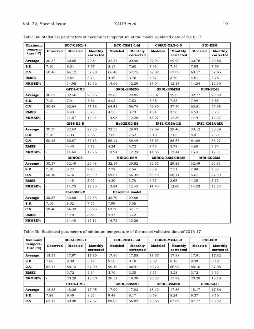
Table 3a: Statistical parameters of maximum temperature of the model validated data of 2016-17

Maximum tempera-ture (oC)

BCC-CSM1-1 BCC-CSM1-1-M CSIro-Mk3-6-0 FIo-eSM

observed Modeled Monthly corrected

Modeled Monthly corrected



average 30.37 32.85 29.84 32.54 29.90 32.94 29.90 32.76 29.86

S.d. 7.10 8.01 7.57 8.15 7.60 7.93 7.56 7.95 7.59

C.v. 50.48 64.12 57.28 66.48 57.75 62.82 57.09 63.17 57.65

rMSe - 4.54 3.74 4.46 3.76 4.57 3.70 4.51 3.76

NrMSe% - 14.95 12.32 14.69 12.39 15.04 12.17 14.84 12.39

gFdL-CM3 gFdL-eSM2g gFdL-eSM2M gISS-e2-h

average 30.37 32.56 29.96 32.85 29.85 33.07 29.85 32.77 29.89

S.d. 7.10 7.91 7.56 8.03 7.53 8.35 7.58 7.99 7.55

C.v. 50.48 62.64 57.18 64.41 56.74 69.80 57.50 63.81 56.98

rMSe - 4.43 3.78 4.55 3.73 4.94 3.76 4.53 3.73

NrMSe% - 14.57 12.44 14.98 12.28 16.27 12.39 14.91 12.27

gISS-e2-r hadgeM2-eS IPSL-CM5a-Lr IPSL-CM5a-Mr

average 30.37 32.63 29.85 32.33 29.83 32.69 29.46 33.12 30.29

S.d. 7.10 7.93 7.56 7.62 7.52 8.10 7.65 8.01 7.50

C.v. 50.48 62.87 57.13 58.11 56.49 65.63 58.57 64.08 56.27

rMSe - 4.45 3.72 4.24 3.72 4.45 3.78 4.68 3.74

NrMSe% - 14.64 12.25 13.94 12.23 14.65 12.44 15.41 12.31

MIroC5 MIroC-eSM MIroC-eSM-CheM MrI-CgCM3

average 30.37 32.49 29.48 32.14 29.82 32.55 29.83 32.49 29.81

S.d. 7.10 8.22 7.78 7.72 7.54 8.09 7.51 7.98 7.58

C.v. 50.48 67.61 60.49 59.57 56.92 65.48 56.44 63.71 57.50

rMSe - 4.48 3.92 4.20 3.78 4.37 3.65 4.35 3.72

NrMSe% - 14.75 12.90 13.84 12.45 14.40 12.00 14.33 12.25

NoreSM1-M ensemble model

average 30.37 32.66 29.86 32.70 29.86

S.d. 7.10 8.02 7.55 7.99 7.56

C.v. 50.48 64.30 56.96 63.76 57.17

rMSe - 4.40 3.68 4.47 3.72

NrMSe% - 14.48 12.11 14.72 12.26

Table 3b: Statistical parameters of minimum temperature of the model validated data of 2016-17

Minimum tempera-ture (oC)






average 18.33 17.97 17.85 17.86 17.88 18.37 17.88 17.91 17.82

S.d. 7.88 9.39 8.19 9.50 8.18 9.52 8.18 9.39 8.19

C.v. 62.17 88.13 67.09 90.19 66.91 90.72 66.92 88.10 67.08

rMSe - 3.72 3.34 3.76 3.35 3.71 3.28 3.72 3.33

NrMSe% - 20.29 18.20 20.51 18.30 20.23 17.92 20.28 18.18


average 18.33 18.26 17.95 17.99 17.83 18.12 17.86 18.17 17.86

S.d. 7.88 9.49 8.23 9.48 8.17 9.68 8.24 9.37 8.16

C.v. 62.17 89.98 67.67 89.85 66.82 93.65 67.89 87.77 66.52


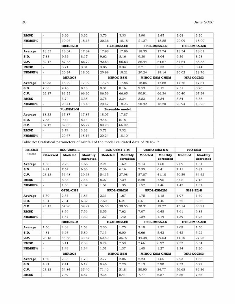
20 June 2020

rMSe - 3.66 3.32 3.73 3.33 3.90 3.45 3.68 3.30

NrMSe% - 19.96 18.13 20.36 18.18 21.27 18.85 20.09 18.00


average 18.33 18.04 17.84 17.98 17.86 18.35 17.74 18.54 18.01

S.d. 7.88 9.36 8.17 9.62 8.16 9.30 8.04 9.36 8.28

C.v. 62.17 87.65 66.72 92.53 66.63 86.44 64.67 87.64 68.58

rMSe - 3.71 3.31 3.85 3.34 3.71 3.33 3.67 3.44

NrMSe% - 20.24 18.06 20.99 18.21 20.24 18.14 20.02 18.76


average 18.33 18.22 17.92 17.78 17.86 18.05 17.88 17.76 17.81

S.d. 7.88 9.46 8.18 9.31 8.16 9.53 8.15 9.51 8.20

C.v. 62.17 89.55 66.90 86.59 66.65 90.91 66.34 90.40 67.24

rMSe - 3.74 3.38 3.75 3.34 3.83 3.34 3.84 3.35

NrMSe% - 20.41 18.46 20.47 18.25 20.92 18.20 20.94 18.25


average 18.33 17.87 17.87 18.07 17.87

S.d. 7.88 9.44 8.14 9.45 8.18

C.v. 62.17 89.03 66.27 89.23 66.92

rMSe - 3.79 3.33 3.71 3.32

NrMSe% - 20.67 18.16 20.24 18.10

Table 3c: Statistical parameters of rainfall of the model validated data of 2016-17

rainfall (mm)






average 1.50 2.25 1.66 2.21 1.62 2.14 1.60 2.09 1.51

S.d. 4.81 7.52 6.30 7.36 6.16 7.55 6.41 7.11 5.87

C.v. 23.13 56.48 39.63 54.15 37.98 57.07 41.10 50.59 34.42

rMSe - 8.38 7.46 8.27 7.39 8.28 7.95 8.05 7.15

NrMSe% - 1.53 1.37 1.51 1.35 1.52 1.46 1.47 1.31


average 1.50 2.57 1.86 2.31 1.67 1.75 1.18 1.97 1.40

S.d. 4.81 7.61 6.32 7.50 6.21 5.51 4.45 6.72 5.56

C.v. 23.13 57.90 39.97 56.30 38.55 30.31 19.77 45.14 30.91

rMSe - 8.56 7.59 8.55 7.62 7.07 6.48 7.61 6.83

NrMSe% - 1.57 1.39 1.57 1.40 1.29 1.19 1.39 1.25


average 1.50 2.03 1.53 2.30 1.75 2.18 1.57 2.09 1.50

S.d. 4.81 6.97 5.80 7.13 6.00 6.66 5.43 6.42 5.22

C.v. 23.13 48.58 33.67 50.89 35.97 44.38 29.53 41.16 27.26

rMSe - 8.11 7.30 8.24 7.50 7.66 6.92 7.33 6.54

NrMSe% - 1.49 1.34 1.51 1.37 1.40 1.27 1.34 1.20


average 1.50 2.35 1.70 2.77 2.06 2.23 1.65 2.23 1.65

S.d. 4.81 7.41 6.12 8.46 7.20 7.13 5.90 7.53 6.27

C.v. 23.13 54.84 37.40 71.49 51.84 50.90 34.77 56.68 39.36

rMSe - 7.69 6.87 9.38 8.41 7.77 6.87 8.56 7.66

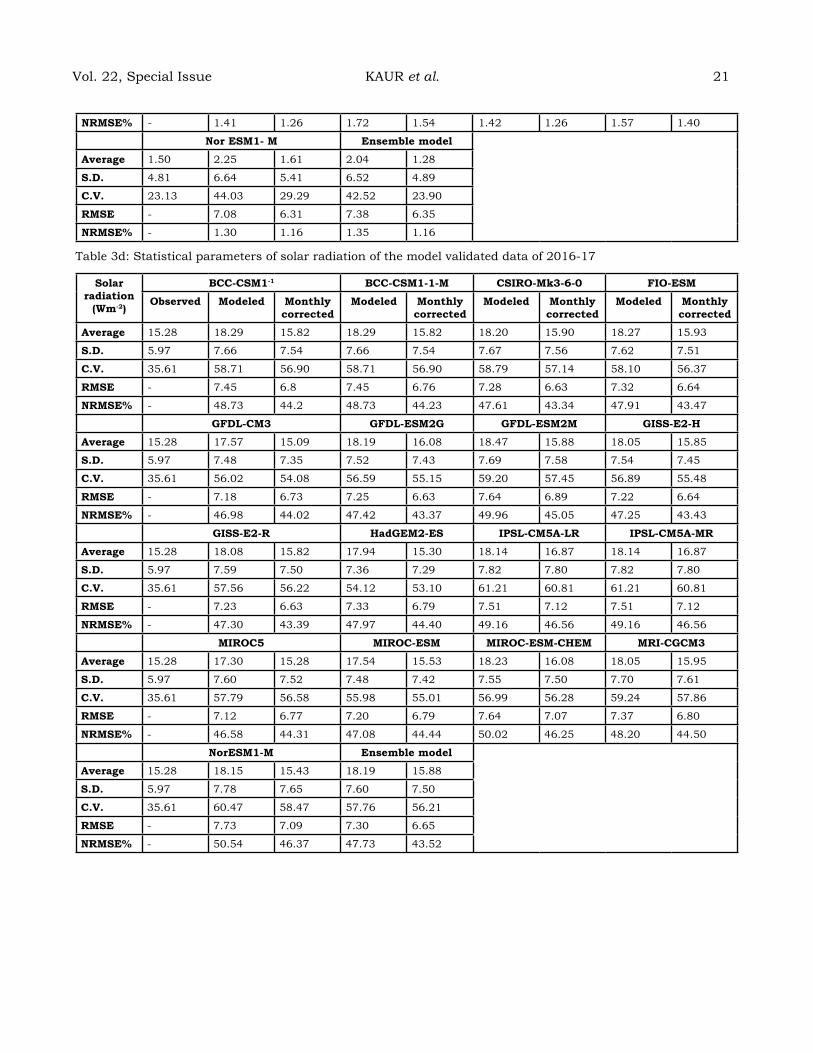
NrMSe% - 1.41 1.26 1.72 1.54 1.42 1.26 1.57 1.40

Nor eSM1- M ensemble model

average 1.50 2.25 1.61 2.04 1.28

S.d. 4.81 6.64 5.41 6.52 4.89

C.v. 23.13 44.03 29.29 42.52 23.90

rMSe - 7.08 6.31 7.38 6.35

NrMSe% - 1.30 1.16 1.35 1.16

Table 3d: Statistical parameters of solar radiation of the model validated data of 2016-17

Solar radiation

(Wm-2)






average 15.28 18.29 15.82 18.29 15.82 18.20 15.90 18.27 15.93

S.d. 5.97 7.66 7.54 7.66 7.54 7.67 7.56 7.62 7.51

C.v. 35.61 58.71 56.90 58.71 56.90 58.79 57.14 58.10 56.37

rMSe - 7.45 6.8 7.45 6.76 7.28 6.63 7.32 6.64

NrMSe% - 48.73 44.2 48.73 44.23 47.61 43.34 47.91 43.47


average 15.28 17.57 15.09 18.19 16.08 18.47 15.88 18.05 15.85

S.d. 5.97 7.48 7.35 7.52 7.43 7.69 7.58 7.54 7.45

C.v. 35.61 56.02 54.08 56.59 55.15 59.20 57.45 56.89 55.48

rMSe - 7.18 6.73 7.25 6.63 7.64 6.89 7.22 6.64

NrMSe% - 46.98 44.02 47.42 43.37 49.96 45.05 47.25 43.43


average 15.28 18.08 15.82 17.94 15.30 18.14 16.87 18.14 16.87

S.d. 5.97 7.59 7.50 7.36 7.29 7.82 7.80 7.82 7.80

C.v. 35.61 57.56 56.22 54.12 53.10 61.21 60.81 61.21 60.81

rMSe - 7.23 6.63 7.33 6.79 7.51 7.12 7.51 7.12

NrMSe% - 47.30 43.39 47.97 44.40 49.16 46.56 49.16 46.56


average 15.28 17.30 15.28 17.54 15.53 18.23 16.08 18.05 15.95

S.d. 5.97 7.60 7.52 7.48 7.42 7.55 7.50 7.70 7.61

C.v. 35.61 57.79 56.58 55.98 55.01 56.99 56.28 59.24 57.86

rMSe - 7.12 6.77 7.20 6.79 7.64 7.07 7.37 6.80

NrMSe% - 46.58 44.31 47.08 44.44 50.02 46.25 48.20 44.50


average 15.28 18.15 15.43 18.19 15.88

S.d. 5.97 7.78 7.65 7.60 7.50

C.v. 35.61 60.47 58.47 57.76 56.21

rMSe - 7.73 7.09 7.30 6.65

NrMSe% - 50.54 46.37 47.73 43.52


22 June 2020

but solar radiation showed decreasing trend after bias removal. Bias correction methods are used extensively in impact assessment studies (Muerth et al., 2013; Teng et al., 2015; Ines and Hansen, 2006). The application of these methods, however, is not without controversy (Ehret et al., 2012). Therefore, the selection of GCM’s was important for better future projections because all the models do not give more reliable results after bias removal. For better future projections of climate change screening of GCM’s models was essential.

Fig 1: Comparison of maximum and minimum temperature, rainfall and solar radiation of observed and modeled data corrected by difference method of bias removal for 2016-17

reFereNCeSAndréasson, J., Bergström, S., Carlsson, B.,

Graham, L.P., and Lindström, G. (2004). Hydrological change–Climate change

impact simulation for Sweden. Ambio., 33: 4-5, 228-234.

Bennett, K.E., Werner, A.T., and Schnorbus, M. (2012). Uncertainties in Hydrologic and Climate Change Impact Analyses in Headwater Basins of British Columbia. Journal of Climate, 25: 17, 5711- 5730, DOI:10.1175/jcli-d-11-00417.1.

Beyene, T., Lettenmaier, D. P., and Kabat, P. (2010). Hydrologic impacts of climate change on the Nile River Basin: implications of the 2007 IPCC scenarios. Climatic Change, 100: 433-461.

Déqué, M., Rowell, D. P., Lüthi, D., Giorgi, F., Christensen, J. H., Rockel, B., Jacob, D., Kjellström, E., De, Castro. M., and van, den. Hurk. B. (2007). An intercomparison of regional climate simulations for Europe: assessing uncertainties in model projections. Climatic Change, 81: 53- 70.

Dingbao, Wang. X. C. (2013). Constructing comprehensive datasets for understanding human and climate change impacts on the hydrologic cycle. Irrigation & Drainage Systems Engineering, 02:01, 1000106. DOI:10.4172/2168-9768.1000106

Ehret, U., Zehe, E., Wulfmeyer, V., Warrach-Sagi, K., and Liebert, J. (2012). HESS Opinions “Should we apply bias correction to global and regional climate model data? Hydrology and Earth System Science, 16: 3391–3404, https://doi.org/10.5194/hess-16-3391- 2012.

Fowler, H. J., Blenkinsop, S., and Tebaldi, C. (2007). Linking climate change modeling to impacts studies: recent advances in downscaling techniques for hydrological modeling. International Journal of Climatology, 27:1547-1578.

Hansen, J. W., Challinor, A., Ines, A., Wheeler, T., and Moronet, V. (2006). Translating forecasts into agricultural terms: advances and challenges, Climate Res 33: 27–41.

Hashino, T., Bradlley, A. A., and Schwartz, S. S. (2007). Evaluation of bias correction methods ensemble stream flow water forecast. Hydrol Earth Syst Sci., 11: 939-950.

IPCC: Climate Change. (2013). The Physical Science Basis. Contribution of Working Group I to the Fifth Assessment Report of the Intergovernmental Panel on Climate

Change, edited by: Stocker, T. F., Qin, D., Plattner, G. K., Tignor, M., Allen, S. K., Boschung, J., Nauels, A., Xia, Y., Bex, V., and Midgley, P. M., Cambridge University Press, Cambridge, United Kingdom, and New York, NY, USA, 1535 pp., https://doi.org/10.1017/CBO97811074153 24.

Ines, A.V.M., and Hansen, J.W. (2006). Bias correction of daily GCM rainfall for crop simulation studies. Agricultural and Forest Meteorology, 138:1-4, 44-53, DOI:10.1016/ j.agrformet. 2006.03.009.

Jamieson, P. D., Porter, J. R., and Wilson, D. R. (1991). A test of computer simulation model ARC-WHEAT1 on wheat crops grown in New Zealand. Field Crops Research, 27, 337–350.

Karl, T., and Trenberth, K. (2003). Modern Global Change. Science., 302: 1719-1722.

Muerth, M., and Coauthors. (2013). On the need for bias correction in regional climate scenarios to assess climate change impacts on river runoff. Hydrology and Earth System

Sciences, 17: 1189-1204.Najafi, M. R., and Moradkhani, H. (2015). Multi-

model ensemble analysis of runoff extremes for climate change impact assessments. Journal of Hydrology, 525: 352-361.

Sharma, D., Das, Gupta. A., and Babel, M. S. (2007). Spatial disaggregation of bias-corrected GCM precipitation for improved hydro-logic simulation: Ping River Basin, Thailand, Hydrol Earth Syst Sci 11: 1373–90.

Taye, M. T., Ntegeka V., Ogiramoi N. P., and Willems, P. (2011). Assessment of climate change impact on hydrological extremes in two source regions of the Nile River Basin. Hydrology and Earth System Sciences, 15: 209-222.

Teng, J., Potter, N., Chiew, F., Zhang, L., Wang, B., Vaze, J., and Evans, J. (2015). How does bias correction of regional climate model precipitation affect modeled runoff? Hydrology and Earth System Sciences, 19: 711-728, DOI:10.5194/hess-19-711-2015.


rainfall probability analysis for crop planning of Jammu region

MaheNder SINgh1, Charu SharMa1, B.C. SharMa*1, r.K.SrIvaStava2, SuShMIta M. dadhICh2, J.P. SINgh2 aNd vIKaS guPta*2

1Agrometeorology Section, *1Division of Agronomy2Division of Agricultural Engineering, *2ACRA, Rakh Dhiansar

Sher-e-Kashmir, University of Agricultural Sciences & Technology of JammuMain Campus, Chatha, Jammu -180009 (J & K)


aBStraCtLong term weekly rainfall data (≥ 30 years) were used for analysis of dry and wet spells at different locations of Jammu region with the help of Markov chain model and normal distribution. The analysis of dry and wet periods during rainy season along coupled with knowledge of onset and withdrawal helps in successful agricultural crop planning with the managing the soil and water conservation measures. In the present study, the chances of occurrences of dry and wet spells at different districts of Jammu using Markov chain probability model. The prediction of weekly initial and conditional rainfall probabilities of receiving at least 10, 20 and 30 mm of rainfall have been studied for effective crop planning of the region. The rainfall characteristics were analyzed on annual, seasonal, monthly and weekly basis. The annual rainfall analysis showed that about 74.0, 77.2, 70.9, 40.8, 38.6, 32.3 percent and 20.5, 18.5, 24.2, 59.1, 61.4, 67.7 percent rainfall received during kharif and rabi season at Jammu, Samba, Katra, Bhaderwah, Batote, Banihal station, respectively. The conditional probability of getting rainfall in two consecutive weeks as a wet (P2W) and dry (P2D) week for a given amount of rainfall (10, 20 and 30 mm) of different stations of Jammu region was analyzed by using long term data.

Keywords: Rainfall, dry, wet spell, conditional probability, seasonal, annual, crop planning.

INtroduCtIoN

Agriculture is the backbone of Indian economy as well as our food and nutritional security. Adverse weather conditions tilt the balance and badly affect the livelihood and food production system. The analysis of rainfall on annual and seasonal will give general idea about the rainfall pattern of the region, whereas the weekly rainfall analysis will be of much use for the agricultural planning. The long-term frequency behavior of wet and dry spells has been used by using Markov chain probability model (Sharma and Singh 2010). In agricultural planning and farm decisions on time of sowing, fertilizer application, inter culture operations and other agricultural operations depends on the rainfall variability in the area. Several studies (Subbulakshmi et al., 2005; Singh et al., 2009; Jat et al., 2010; Nemichandrappa et al., 2010; Pawar et al., 2015) reported the weekly rainfall probabilities advantages of working out for a station or an agro-climatic region. In rainfed condition the yield of crops depends on the rainfall pattern. Many researchers has studied the probable behavior of rainfall (Medhi, 1976; Robertson, 1982; Kumar et al., 2007; Jat et al., 2010; Chand et al., 2011). Predicting occurrence

of rainfall events the with the available data using statistical methods or probability analysis used in day to day farm operations (Kumar and Kumar, 1989). Chattopadhyay and Ganesan (1995) studied the probability of occurrence of wet and dry spells on weekly, monthly, seasonal and annual basis rainfall during North–East monsoon season for various stations in Tamil Nadu. In command area, the wet and dry spell analysis will help in cropping system planning characterization of crop and designing of conservation structures. The probability of rain during next week, if rain occurs this week known as conditional probability of a wet week preceded by a wet week (PWW), and the probability of rain next week being wet, if this week is dry known as conditional probability of a wet week preceded by a dry week (PWD). The concept of probability is usually used to study the dry and wet spells for agricultural planning (Srivastava et al., 2004). The initial and conditional probability approach would be relatively good method for rainfall analysis, especially in the regions where rainfall is erratic or where short dry periods can be expected within the wet season. Gupta et al. (1975) suggested that the rainfall at 80 per cent probability can safely be taken as assured rainfall, while that of 50 per


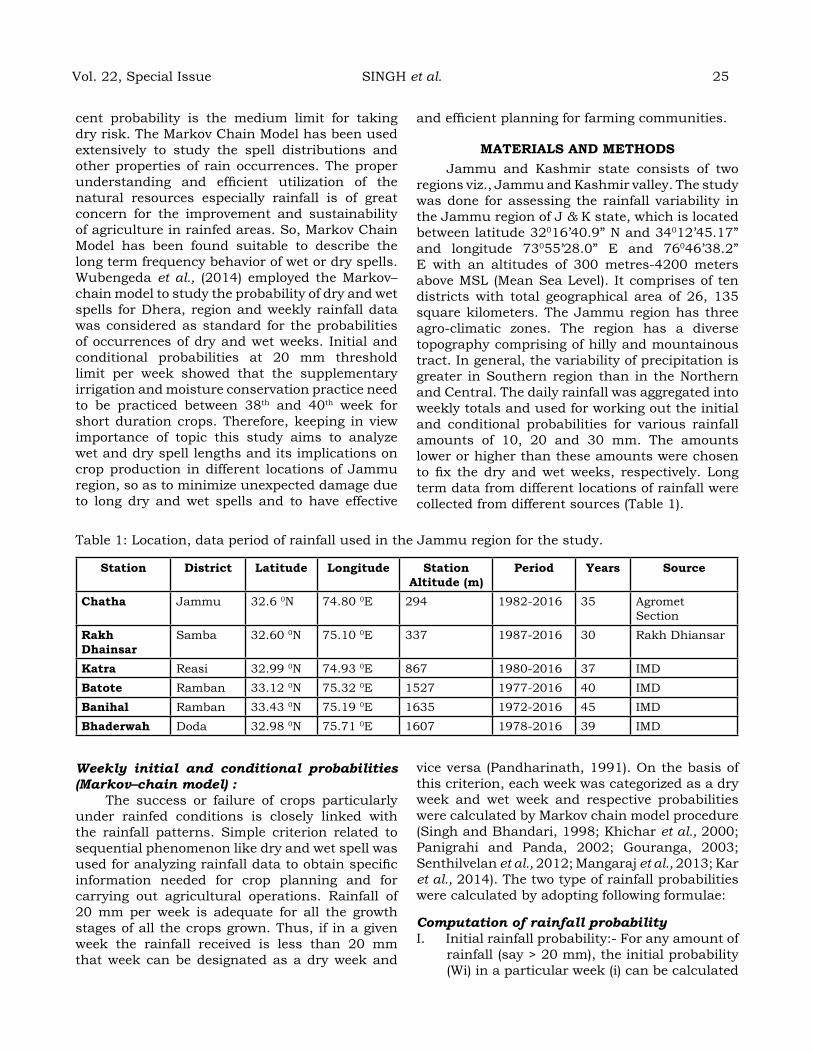
cent probability is the medium limit for taking dry risk. The Markov Chain Model has been used extensively to study the spell distributions and other properties of rain occurrences. The proper understanding and efficient utilization of the natural resources especially rainfall is of great concern for the improvement and sustainability of agriculture in rainfed areas. So, Markov Chain Model has been found suitable to describe the long term frequency behavior of wet or dry spells. Wubengeda et al., (2014) employed the Markov–chain model to study the probability of dry and wet spells for Dhera, region and weekly rainfall data was considered as standard for the probabilities of occurrences of dry and wet weeks. Initial and conditional probabilities at 20 mm threshold limit per week showed that the supplementary irrigation and moisture conservation practice need to be practiced between 38th and 40th week for short duration crops. Therefore, keeping in view importance of topic this study aims to analyze wet and dry spell lengths and its implications on crop production in different locations of Jammu region, so as to minimize unexpected damage due to long dry and wet spells and to have effective

and efficient planning for farming communities.

MaterIaLS aNd MethodSJammu and Kashmir state consists of two

regions viz., Jammu and Kashmir valley. The study was done for assessing the rainfall variability in the Jammu region of J & K state, which is located between latitude 32016’40.9” N and 34012’45.17” and longitude 73055’28.0” E and 76046’38.2” E with an altitudes of 300 metres-4200 meters above MSL (Mean Sea Level). It comprises of ten districts with total geographical area of 26, 135 square kilometers. The Jammu region has three agro-climatic zones. The region has a diverse topography comprising of hilly and mountainous tract. In general, the variability of precipitation is greater in Southern region than in the Northern and Central. The daily rainfall was aggregated into weekly totals and used for working out the initial and conditional probabilities for various rainfall amounts of 10, 20 and 30 mm. The amounts lower or higher than these amounts were chosen to fix the dry and wet weeks, respectively. Long term data from different locations of rainfall were collected from different sources (Table 1).

Table 1: Location, data period of rainfall used in the Jammu region for the study.

Station district Latitude Longitude Station altitude (m)

Period Years Source

Chatha Jammu 32.6 0N 74.80 0E 294 1982-2016 35 Agromet Section

rakh dhainsar

Samba 32.60 0N 75.10 0E 337 1987-2016 30 Rakh Dhiansar

Katra Reasi 32.99 0N 74.93 0E 867 1980-2016 37 IMD Batote Ramban 33.12 0N 75.32 0E 1527 1977-2016 40 IMDBanihal Ramban 33.43 0N 75.19 0E 1635 1972-2016 45 IMDBhaderwah Doda 32.98 0N 75.71 0E 1607 1978-2016 39 IMD

Weekly initial and conditional probabilities (Markov–chain model) :

The success or failure of crops particularly under rainfed conditions is closely linked with the rainfall patterns. Simple criterion related to sequential phenomenon like dry and wet spell was used for analyzing rainfall data to obtain specific information needed for crop planning and for carrying out agricultural operations. Rainfall of 20 mm per week is adequate for all the growth stages of all the crops grown. Thus, if in a given week the rainfall received is less than 20 mm that week can be designated as a dry week and

vice versa (Pandharinath, 1991). On the basis of this criterion, each week was categorized as a dry week and wet week and respective probabilities were calculated by Markov chain model procedure (Singh and Bhandari, 1998; Khichar et al., 2000; Panigrahi and Panda, 2002; Gouranga, 2003; Senthilvelan et al., 2012; Mangaraj et al., 2013; Kar et al., 2014). The two type of rainfall probabilities were calculated by adopting following formulae:

Computation of rainfall probabilityI. Initial rainfall probability:- For any amount of

rainfall (say > 20 mm), the initial probability (Wi) in a particular week (i) can be calculated

Vol. 22, Special Issue SINGH et al. 25

26 June 2020

as:No. of years during which rainfall in the i week > 20 mm

Wi= -------------------------------------------------------------------- x 100Total number of year

II. Conditional rainfall probability of wet weeks followed by wet weeks (W/W) and dry weeks followed by dry weeks (D/D) :

The initial and conditional probability analysis was carried out for wet weeks and dry week threshold amounts of 10, 20 and 30 mm weekly rainfall for standard week 01 to 52 (1st January to 31st December).

Conditional rainfall probability (%) of getting any amount of rainfall (say > 20 mm) during next week (i+1) also when there was rainfall of > 20 mm during this week (i) were calculated as:

No. of years during which next week (i+1) received > 20 mm rainfall when this week (i) also received > 20 mm rainfall

W/Wi= -------------------------------------------------------------------- x 100No. of years during which this week (Wi) received > 20 mm

rainfall

The initial and conditional probability analysis was done for wet week threshold value of 30, 20 and 10 mm weekly rainfall. The initial and conditional rainfall probability for rainfall amount of 30, 20 and 10 mm were computed during kharif and rabi season on standard meteorological week wise for various locations of Jammu region. The probability of rain during next week, if rain occurs this week known as conditional probability of a wet week preceded by a wet week (PW/W) denoted by P2W, and the probability of rain next week being wet, if this week is dry known as conditional probability of a dry week preceded by a dry week (PD/D) and is denoted by P2D.

Descriptive and time series analyses were used to depict the temporal distribution of rainfall. The standard deviation (S.D) and Coefficient of Variation (CV) of rainfall were worked out for crop growing season and on annual basis for various locations of Jammu region. Coefficient of mean deviation was calculated by adopting the formulae that the ratio of mean deviation of the mean or average to the mean and multiply by 100 or in other form D (Percent) = [ ( (A-N) /N) *100].

reSuLtS aNd dISCuSSIoNAnnual Rainfall distribution

The mean annual rainfall variability of Jammu region varies from 1133.3 to 2014.0 mm with a standard deviation (SD) observed between 234.2 to 439.2 mm and the coefficient of variation (CV) differs from 19.5 to 26.0 percent. The mean annual

rainfall of different locations viz; Jammu, Samba, Katra, Batote, Bhaderwah and Banihal were found 1159.7, 1133.3, 2014.0, 1606.1, 1282.7 & 1360.4 mm with standard deviation (S.D.) of 241.6, 234.2, 439.2, 353.2, 252.0 & 343.3 mm and coefficient of variation (C.V.) of about 21.3, 21.3, 21.3, 21.9, 19.5 & 25.8 percent, respectively (Table 2). Out of this, more than 70 to 78 percent of annual rainfall was received during kharif season (June to September) and only 18 to 25 percent received during rabi season at Jammu, Samba and Katra locations. Whereas, at mid to high altitude areas like Bhaderwah, Batote and Banihal, 25.0 to 33.0 percent annual rainfall received during kharif season and 56.8 to 68 percent during rabi season (Table 2). In sub-tropical region (Jammu & Samba) and intermediate region (Katra) of Jammu division the standard deviation and coefficient of variation were lower as compared to temperate region (Bhaderwah, Batote & Banihal) during kharif season, while during rabi season C.V. was found more at Jammu, Samba, Katra as compared to Batote, Bhaderwah and Banihal (Table 2). The coefficient of variation (CV) in percentage is an indicative of dependability of rainfall. The threshold levels for CV for any interpretation are < 25, < 50, < 100 and < 150 per cent for annual, seasonal, monthly and weekly rainfall respectively (Manorama et al., 2007).

Seasonal rainfall distributionThe meteorological as well as crop season

wise rainfall distribution were analyzed in order to compare the inter seasonal rainfall variability and its pattern in the region and is presented in Table 2. The results showed highest rainfall received during monsoon (kharif) season (70 to 78 percent) followed by pre monsoon (10 to 13 percent), winter season (9 to 11 percent) and post monsoon season (04 to 06 percent) at Jammu, Samba and Katra locations. While, Batote and Bhaderwah station has received only 33 and 36 percent of the annual rainfall during monsoon or kharif season and followed by pre-monsoon season which received 32 and 30 percent, respectively. Whereas, 24 and 10 percent of the annual rainfall were occurred during winter and post monsoon season, respectively. But Banihal station has received higher rainfall during pre-monsoon (33.0 percent) followed by winter (29.0 percent), monsoon (25.0 percent) and post monsoon season (13.0 percent). The sub-tropical and intermediate zone (Jammu, Samba and Katra) received very less rainfall (18.3 to 22.5 percent) during rabi season

Table 2: Statistical parameters of annual and seasonal (meteorological and crop season wise) rainfall of different seasons at different stations of Jammu region.

Mean (mm)

S.d (mm)

C.v (%)

PC highest rain (mm)

Lowest rain (mm)

JammuAnnual Rainfall 1159.7 241.6 21.3 100 1824.9 (1990) 830.3 (2001) Winter Rainfall (Jan-Feb) 101.4 60.1 59 9 244.2 (2005) 13.9 (2001) Pre Monsoon (March-May) 128.9 109.0 84 11 502.7 (2015) 34.2 (1999) Monsoon/Kharif (June-Sept) 881.2 207.2 24 76 1265.9 (2005) 457.5 (2001) Post Monsoon (Oct-Dec) 48.4 42.4 88 4 142.0 (1990) 0.0 (1993, 2005) Rabi Season (Oct-March) 231.4 134.4 56.0 20 620.0 (1989-90) 36.7 (2000-01) SambaAnnual Rainfall 1133.3 234.2 23.1 100 1824.9 (1990) 754.1 (2009) Winter Rainfall (Jan-Feb) 96.9 57.3 59 9 243.3 (2005) 13.9 (2001) Pre Monsoon (March-May) 113.3 86.2 76 10 438.2 (1990) 29.3 (2013) Monsoon/Kharif (June-Sept) 878.6 204 23 78 1264.3 (2011) 514.1 (1987) Post Monsoon (Oct-Dec) 44.5 40 90 4 620.0 (1989-90) 36.7 (2000-01) Rabi Season (Oct-March) 207.9 128.9 64.2 18.3 620.0 (1989-90) 36.7 (2000-01) KatraAnnual Rainfall 2014.0 439.2 21.3 100 3179.3 (1988) 1365.0 (1987) Winter Rainfall (Jan-Feb) 237 130 55 11 488.9 (2005) 10.0 (2001) Pre Monsoon (March-May) 264 141 54 13 671.6 (1982) 78.2 (1999) Monsoon/Kharif (June-Sept) 1454 392 27 70 2486.3 (1988) 715.9 (1987) Post Monsoon (Oct-Dec) 115 83 72 6 333.1 (1986) 0.0 (1993) Rabi Season (Oct-March) 453.6 206.2 44.5 22.5 777.8 (1997-98) 51.0 (2000-01) BatoteAnnual Rainfall 1606.1 353.2 21.9 100 2253.5 (2015) 966.7 (2001) Winter Rainfall (Jan-Feb) 393 159 40 24 860.3 (2005) 65.0 (2001) Pre Monsoon (March-May) 517 221 43 32 1032.4 (1990) 214.5 (2004) Monsoon/Kharif (June-Sept) 528 199 38 33 1118.3 (1988) 275.1 (1982) Post Monsoon (Oct-Dec) 168 112 66 10 426.0 (1994) 42.6 (2000) Rabi Season (Oct-April) 970.2 272.1 27.4 60.4 1423.2 (1997-98) 389.3 (2000-01) BhaderwahAnnual Rainfall 1282.7 252.0 19.5 100 2006.0 (1988) 747.4 (2009) Winter Rainfall (Jan-Feb) 307 143 47 24 701.0 (1990) 71.9 (2009) Pre Monsoon (March-May) 386 130 34 30 715.0 (1983) 166.7 (1999) Monsoon/Kharif (June-Sept) 458 155 34 36 951.0 (1988) 229.0 (1982) Post Monsoon (Oct-Dec) 133 66 49 10 445.2 (1986) 45.8 (1993) Rabi Season (Oct-April) 728.8 226.1 30.9 56.8 1198.9 (1989-90) 323.1 (2008-09) BanihalAnnual Rainfall 1360.4 343.3 25.8 100 2138.7 (2015) 707.9 (2001) Winter Rainfall (Jan-Feb) 392 169 43 29 915.0 (2005) 92.9 (2001) Pre Monsoon (March-May) 448 203 45 33 792.8 (1987) 145.5 (2008) Monsoon/Kharif (June-Sept) 345 171 49 25 869.0 (1975) 102.8 (1993) Post Monsoon (Oct-Dec) 176 125 71 13 536.8 (1994) 17.4 (1975) Rabi Season (Oct-April) 930.9 236.7 26.0 68 1367.3 (2004-05) 390.7 (1998-99) S.D.= Standard Deviation (± mm) ; CV Coefficient of Variation (percent), PC= Percent contribution (percent), Rabi season: Oct- March in subtropical region; Oct to April in intermediate region


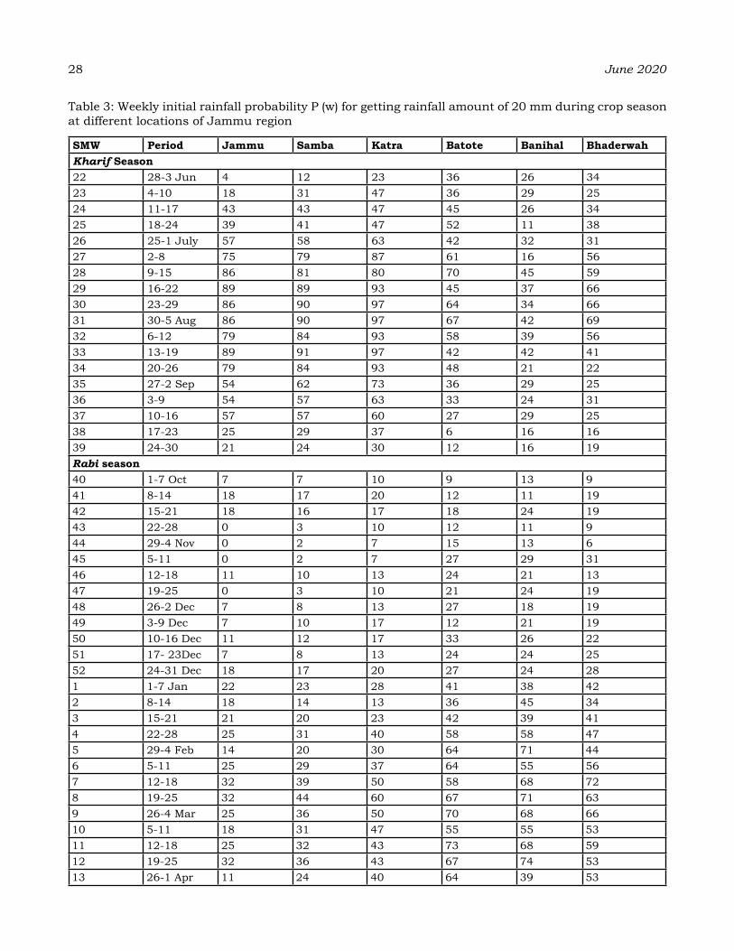
28 June 2020

Table 3: Weekly initial rainfall probability P (w) for getting rainfall amount of 20 mm during crop season at different locations of Jammu region

SMW Period Jammu Samba Katra Batote Banihal BhaderwahKharif Season22 28-3 Jun 4 12 23 36 26 3423 4-10 18 31 47 36 29 2524 11-17 43 43 47 45 26 3425 18-24 39 41 47 52 11 3826 25-1 July 57 58 63 42 32 3127 2-8 75 79 87 61 16 5628 9-15 86 81 80 70 45 5929 16-22 89 89 93 45 37 6630 23-29 86 90 97 64 34 6631 30-5 Aug 86 90 97 67 42 6932 6-12 79 84 93 58 39 5633 13-19 89 91 97 42 42 4134 20-26 79 84 93 48 21 2235 27-2 Sep 54 62 73 36 29 2536 3-9 54 57 63 33 24 3137 10-16 57 57 60 27 29 2538 17-23 25 29 37 6 16 1639 24-30 21 24 30 12 16 19Rabi season 40 1-7 Oct 7 7 10 9 13 941 8-14 18 17 20 12 11 1942 15-21 18 16 17 18 24 1943 22-28 0 3 10 12 11 944 29-4 Nov 0 2 7 15 13 645 5-11 0 2 7 27 29 3146 12-18 11 10 13 24 21 1347 19-25 0 3 10 21 24 1948 26-2 Dec 7 8 13 27 18 1949 3-9 Dec 7 10 17 12 21 1950 10-16 Dec 11 12 17 33 26 2251 17- 23Dec 7 8 13 24 24 2552 24-31 Dec 18 17 20 27 24 281 1-7 Jan 22 23 28 41 38 422 8-14 18 14 13 36 45 343 15-21 21 20 23 42 39 414 22-28 25 31 40 58 58 475 29-4 Feb 14 20 30 64 71 446 5-11 25 29 37 64 55 567 12-18 32 39 50 58 68 728 19-25 32 44 60 67 71 639 26-4 Mar 25 36 50 70 68 6610 5-11 18 31 47 55 55 5311 12-18 25 32 43 73 68 5912 19-25 32 36 43 67 74 5313 26-1 Apr 11 24 40 64 39 53

as compared to intermediate to temperate zone (Batote, Bhaderwah and Banihal) of about 56.8 to 68.0 percent (Table 2). During kharif season, the rainfall showed the increasing trends at the rate of 1.954, 0.383, 2.804, 0.121 and 0.121 mm per year at Jammu, Samba, Bhaderwah, Batote and Banihal, respectively. At Katra station, the rainfall decreases at the rate of 0.213 mm per year during monsoon season. But during rabi season the rainfall trends was increasing at Jammu, Banihal and Batote with the rate of 1.252, 1.224 and 1.224 mm year, respectively, while decreasing in Katra, Samba & Bhaderwah at the rate of 3.306, 0.142 and 7.257 mm per year, respectively (Table 2).

Study of yearly variation in rainfall

Fig. 1: Mean deviation (percent) from the normal rainfall in different years at various locations in Jammu region

Annual rainfall of station wise showed a lot of variation. For this a year wise coefficient of mean deviation (± per cent) was calculated and presented in Fig. 1. The results revealed that the rainfall variability of 36 years of data varies from -30.1 to 63.6 percent from average annual rainfall in Jammu district. Out of these 36 years of study about 7 years (1987, 1989, 1999, 2002, 2004, 2005 & 2009) have more than 20 percent deficient


30 June 2020

rainfall received, however, the surplus rainfall (≥20 percent) was received in another 7 years (1986, 1990, 1996, 1997, 2003, 2012 & 2015). In rest of 20 years the average annual rainfall received between -19 to +19 percent deviations in Jammu district (Fig. 1). At Samba location out of 30 years of rainfall data shows the variability varies from -34.1 to 59.6 percent. The maximum deficient and surplus rainfall amounts were found in 2009 (-34.1 percent) and 1990 (+59.6 percent). The 5 years were found deficient, while 5 years have surplus rainfall among these 30 years of study. In this district more than 70 percent areas under rainfed farming with undulating topography (Fig. 1).

In intermediate (Katra) regions the highest annual rainfall received as compared to other locations of the current study. The rainfall variability varied from -34.3 to 53.6 percent during last 37 years, out of these the 7 years have got deficient (≥-20 percent), while in 5 years was surplus (≥20 percent) rainfall and rest have around to normal (-19 to 19 percent) rainfall received.

In Bhaderwah, Banihal and Batote (temperate region) the rainfall variability varies from -42.8 to 53.6, -47.3 to 59.2 and -40.5 to 49.8 percent during 39th, 45th and 40th year, respectively. The numbers of years with deficient and excess (≥20 percent) rainfall were three, ten, six and six, nine, seven in Bhaderwah, Banihal, Batote, respectively (Fig. 1).

Initial probability based crop planning during crop season wise

Weekly initial wet P (W) probabilities for getting more than 20 mm rainfall were worked out during the kharif and rabi seasons for Jammu, Samba, Katra, Batote, Banihal, Bhaderwah and are depicted in Table 3. The initial rainfall probability P (W) of getting weekly rainfall of 20 mm was found 40 to 60 per cent during 24th to 26th SMW at Jammu and Katra station and hence, field preparation for sowing of kharif crops (maize, direct sown rice, moong, mash and til) can be done during this period.

The initial weekly rainfall probability P (W) of getting wet week of 20 mm was more than 70 per cent during 27th to 34th SMW and more than 50 per cent during 26th to 37th SMW at Jammu, Samba and Katra stations which shows potentiality for rain water harvesting and similar results reported by Singh et al., (2008). Therefore, this period is

identified as the safer period for the growing of rainfed kharif crops (maize, sesame, moong, mash, cowpeas, sorghum) at Jammu, Samba and Katra stations because moisture sensitive growth stages of these crops not much suffer from the moisture stress. But the high water requirement crops (normal rice, basmati rice and sugarcane) can also be grown at low lying areas of these locations during this period as the sufficient rainfall available in order to meet out optimum production requirement (Table 2).

In intermediate to temperate hill zone station of Jammu province viz; Batote, Banihal and Bhaderwah, the initial rainfall probability of getting weekly rainfall of amount 20 mm was found 18 to 24 per cent during 42nd SMW, which was sufficient for sowing of rabi pulses and oilseed crops in those areas. The probability of 25 to 30 per cent during 45th SMW is suitable for sowing of rabi season crops viz., wheat, barley, oats. The initial rainfall probability is 20 to 30 percent during 50th and 51st week which coincides with crown initiation stage (critical stage of irrigation) of normal sown wheat crop. Gouranga, 2003 also reported such types of results for West Bengal. During 11th and 12th SMW, the normal sown wheat crop is at anthesis stage in which the probability of wet spell is ranged between 50 to 70 per cent (Fig. 2).

Conditional probability of dry and wet spell based week wise crop planning

The conditional probability of dry week followed by dry week (PD/D) and wet week followed by wet week (PW/W) for a given amount of rainfall (10, 20 and 30 mm) of different locations of Jammu region for the 52 standard meteorological weeks was analyzed by using long term data and is presented in Fig. 2.

The conditional probability of getting wet week followed by consecutive wet week was very high during the monsoon/ kharif season of subtropical (Jammu and Samba) and intermediate regions (Katra). The cumulative rainfall amount of 30 mm has found highest from 28th to 32 SMW whereas the probability of cumulative rainfall of 10 and 20 mm in consecutive weeks found maximum from 26th to 34th SMW under subtropical areas of Jammu region. The conditional probability of getting wet week followed by wet week during the monsoon/ kharif season (26th to 33rd SMW) was found between 72 to 94, 50 to78 and 31to 72 per

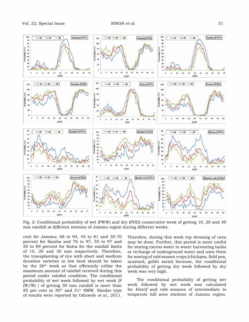
Fig. 2: Conditional probability of wet (PWW) and dry (PDD) consecutive week of getting 10, 20 and 30 mm rainfall at different stations of Jammu region during different weeks.

cent for Jammu; 68 to 94, 45 to 81 and 30-70 percent for Samba and 76 to 97, 55 to 97 and 50 to 89 percent for Katra for the rainfall limits of 10, 20 and 30 mm respectively. Therefore, the transplanting of rice with short and medium duration varieties in low land should be taken by the 26th week so that efficiently utilize the maximum amount of rainfall received during this period under rainfed condition. The conditional probability of wet week followed by wet week {P (W/W) } of getting 30 mm rainfall is more than 85 per cent in 30th and 31st SMW. Similar type of results were reported by Oduwole et al., 2011.

Therefore, during this week top dressing of urea may be done. Further, this period is more useful for storing excess water in water harvesting tanks or recharge of underground water and uses them for sowing of rabi season crops (chickpea, field pea, mustard, gobhi sarso) because, the conditional probability of getting dry week followed by dry week was very high.

The conditional probability of getting wet week followed by wet week was calculated for kharif and rabi seasons of intermediate to temperate hill zone stations of Jammu region.


32 June 2020

A Markov Chain Model for wet and dry spell probabilities at Yola, Adamawa state, Nigerian Journal of Pure & Applied Sciences, ISSN 0795- 25070, Vol 4, pp. 118-125.

Pandharinath, N. (1991). Markov chain model probability of dry, wet weeks during monsoon period over Andhra Pradesh. Mausam., 42: 393 - 400.

Panigrahi, B. and Panda, S.N. (2002). Dry spell probability by Markov chain model and its application to crop planning in Kharagpur. Ind. J. Soil Conserv., 30 (1) : 95-100.

Pawar, P.B., Jadhav, J.D., Patil, S. R. and Amruthsagar, V. M. (2015). Weekly rainfall variability and probability analysis for Solapur in respect of crop planning. Ecoscan, 9 (1-2) : 115- 120.

Robertson, G.W. 1982. Frequency and probability of dry and wet spells. WMO Tech. Nore No. 179:149-153.

Senthilvelan, A., Ganesh, A. and Banukumar, K. (2012). Morkov chain model for probability of weekly rainfall in Orthanadu. Internat. J. Geomatics & Goescie., 3 (1) : 191- 203.

Singh, M. and Bhandari, A.R. (1998). Wet and dry spells analysis using Markov chain model for mid hill region of Himachal Pradesh.

Indian J. Soil Conserv., 26: 147-152.Singh K. A., Sikka A. K. and Rai S. K. (2008).

Rainfall distribution pattern and crop planning at Pusa in Bihar, J.of Agromet., 10 (2) : 198- 203.

Singh, P.K., Rathore, L.S., Singh, K.K., Baxla, A.K. and Athiyaman, B. (2009). Incomplete gamma distribution of rainfall for sustainable crop production strategies at Palampur, Himachal Pradesh. Mausam, 60 (1) : 73-80.

Srivastava, A.K., Sastri, C.V.S. and Garg, R.N. (2004). Rainfall analysis and crop planning in Uttar Pradesh. Ann. of Agril. Res., 25 (2) : 257-264.

Sharma, M.A. and Singh, J.B., (2010). Use of probability distribution in rainfall Analysis. New york sci. J., 3 (9).

Subbulakshmi, S., Selvaraju, R. and Manickasundaram, S. (2005). Rainfall probability analysis for crop planning in selected locations of Tamil Nadu. Madras Agric. J., 92 (1-3) :76-83.

Wubengeda, A., Kassu, T., Fitsume, Y. and Birhan, A. (2014). Markov chain analysis of dry, wet weeks and statistical analysis of weekly rainfall for agricultural planning at Dhera, central rift valley region of Ethiopia. African J. Agric. Res., 9 (29) : 2205-2213.

regional Crop Yield estimation System (rCYeS) using a crop simulation model dSSat v4.7: concept, methods, development, and validation

g. B. gohaIN b, *, K.K. SINgh a, r.S. SINgh b, PrIYaNKa SINgh a

aAgromet Advisory Service Division, India Meteorological Department, New DelhibBanaras Hindu University, Varanasi

Corresponding author’s e-mail: [email protected]

aBStraCtThe crop simulation model simulates the plants process and estimate the yield as function of weather conditions, soil, and crop management information. Global and reliable crop simulation model DSSAT (Decision Support System for Agrotechnology Transfer) is widely used in the modeling of agriculture system by the Research community. This crop model work satisfactorily at a homogeneous farm-scale and need to be incorporated into higher-order systems such as whole farm, catchment, or region. Regional Crop Yield Estimation System (RCYES) is a new approach to attempt the simulation of crop yield at a spatial level using DSSAT codes as basic framework. A framework developed here in Python to optimize the efficient use of the DSSAT crop model at a regional scale. The framework consist of different tools found necessary to prepare required crop model inputs, executing the crop simulation model, reading the crop simulation output, and analyzing the output result. Input data preparation and simulation for all the major crops incorporated in DSSAT can be done with this module. Python scripts were used to develop the tools which are a reliable scientific modeling approach, efficient, timely, and robust framework for the Research and modeling community.

Keywords: DSSAT; Crop Simulation Model; Framework, Tools; Data; Python.

INtroduCtIoN

The DSSAT (DSSAT-CSM, Jones, et al., 2003) crop simulation model is estimated to have more than 2000 users across different countries worldwide (Koo, 2016) and can be used for yield estimation. The DSSAT global crop growth simulation model is used extensively by researchers all over the world since it provides flexibility to the user. These are the mathematical functional models representing the interaction between crop growth processes and the environment. DSSAT v2.1 was first released in 1989. DSSAT originally was developed by an international network of scientists in which they were cooperating in the Agrotechnology Transfer project. Researchers and professionals were using DSSAT model for more than 20 years all over the world, for a variety of purposes, including crop management (Fetcher et al., 1991), climate change and its impact studies (Lal et al. 1998, Saseendran et. al., 2000, Alexandrov and Hoogenboom, 2001, Patel et al., ), introducing Machine learning-Decision tree and Random forest to predict the crop yield (Gohain et al., J. Chen et al., S Fukuda et al., ). There are several types of research has been carried out to increase the efficiency of crop simulation model

by assimilating satellite data into the crop growth models such as APSIM (Keating et al., 2003), CERES (Jones et al., 2003), WOFOST (Van Diepen et al., 1989), Agricultural production is the total of the consequences of the decisions taken by millions of farmers operating across the country in a diverse conditions. The standard user runs the DSSAT software application, a windows-based Graphical user interface (GUI) which has various tools to prepare input files for running simulation and deriving the output. DSSAT-CSM user interface gives the accessibility for beginners, however, the most advanced user of DSSAT-CSM is to develop scripts using programming languages or using a software environment (e.g. R, Python, MATLAB, SAS, FORTRAN, etc.) to automate numerous stages in the analysis for the crop simulation model. Advance estimates of crop yield required reliable and timely crop yield forecasting, which helps the Researcher, insurers, reinsurers, and policymaker’s inappropriate decision making on economic strategies. An approach to developing a framework will enhance the transparency, efficiency, and reproducibility of the use of crop modeling. Python workflow for DSSAT i.e. pyDSSAT (He et al., 2015) is a software package that was developed so that the DSSAT


34 June 2020

crop simulation model can be used efficiently. jDSSAT (Abreu Resenes et al., 2019) which was developed in java Module to replace the existing DSSAT software application. Similarly, we developed a framework for DSSAT using Python i.e. RCYES ( Regional Crop Yield Estimation System), which will execute crop models at different spatial resolutions and analyze the output. To use the DSSAT model efficiently with the large variable weather, management practices, and different environmental modification an automated module is required which simulate crop model different r.t to spatial resolution, different crops, seasons, and post-process the results. RCYES tools developed have pre- and post-processing modules. Pre-processing modules prepare weather and crop experiments in the DSSAT Model format and post-processing for analysis of data after model evaluation.

MaterIaL aNd MethodSAbout Crop Simulation Model (DSSAT v4.7)

Crop growth simulation modeling is a useful tool to describe continuous crop growth and to estimate crop yield using environmental inputs, DSSAT (Decision Support System for Agro Technology Transfer) is used extensively in addition to the other models such as WOFOST, Info Crop, etc. DSSAT is a decision support system that is designed to aid farmers in developing long-term crop rotational strategies for 42 crops as accessible in DSSAT version 4.7 (Hoogenboom et al., 2019). The crop models are developed to assess the influence of weather and management practices (cultivar selection, sowing time and depth, plant population, initial condition, irrigation water, nitrogen schedule, mulching, etc.) on crop growth and development daily. A significant feature of DSSAT is the development of standards for data collection and formats for data acquisition and exchange. This allows any crop model of the family to share and access common soils and weather data. Applications of system approach using comprehensive models like DSSAT to represent the total agricultural production systems require datasets on the different components, namely: (a) crop (b) weather (c) soil and (d) crop management. Models require cultivar specific genetic coefficients for better estimation. These coefficients vary among the crop varieties in response to weather, soil, and management practices. Estimation of genetic coefficients, hence, is vital in crop yield forecasting models.

ModeL INPutSWeather Data

Weather data is one of the important key factors to drive the crop simulation model. IMD gridded data (.GRD), are used to test the weather module and prepare the weather file in the model required format. IMD gridded Rainfall data (Pai et al. 2014), and Temperature data (Srivastava et. al.2009) available in is binary format is used here. Daily gridded data for temperature (maximum and minimum) and Rainfall is available online and can be downloaded in real-time from the India Meteorological Department website. Weather data are extracted using the Weather download module to prepare the data for the crop model. The temperature data is available in 0.50 X 0.50 (~50km grid size) and Rainfall is available in 0.250 X 0.250 (~25km grid size)

Soil DataDSSAT-CSM requires soil data parameters

that characterize the soil texture, structure, depth, profile, level of soil nutrients, and other related variables that describe the soil-water balance and nutrient dynamics during crop growth and development. Soil physical characteristics such as hydraulic conductivity determine the movement of water in the soil. Besides, field capacity, wilting point, the thickness of root zone, bulk density, and water table depth, soil texture, soil depth, pH, EC and slope of soil, etc. are also required. Gridded soil file freely available with Harvard data verse available at 10-km spatial resolution. 25km grid is assigned with a 10km spatial resolution considering the mid soil profile falling under the grid. User can use their dataset at 25km resolution as well.

Crop Management informationCrop management information has different

parameters, which include, crop field, initial soil condition, crop planting area, crop planting details, Irrigation, and Fertilizer applied. Currently, for crop management, it includes the date of planting and harvesting, date of applying inorganic fertilizer and irrigation, crop residue, and organic material. Provision for automatic sowing also inbuilt, which is based on the thresholds/cutoff cumulative rainfall or soil moisture value. For the Indian region, crop experiment data can be prepared using the reference of the FASAL project Report (Singh et al., 2017). Eg for Jalgaon Sowing window is considered between the end of May and mid of July. If the threshold rainfall amount is reached to

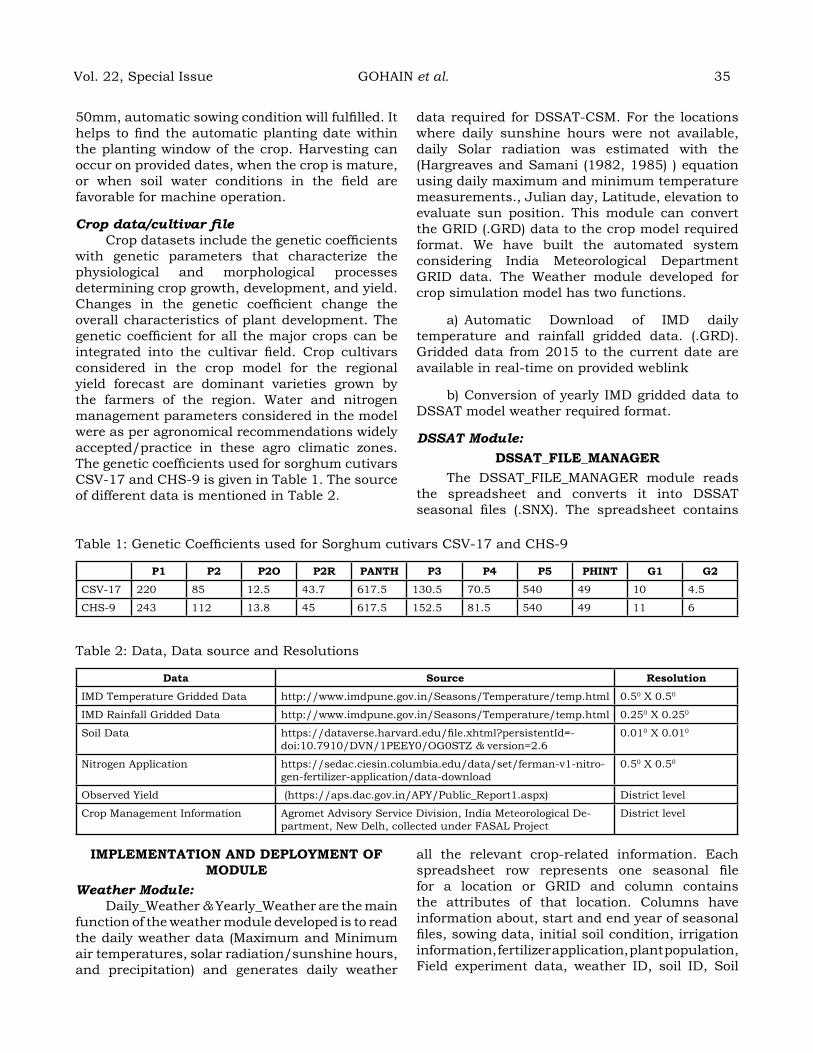
50mm, automatic sowing condition will fulfilled. It helps to find the automatic planting date within the planting window of the crop. Harvesting can occur on provided dates, when the crop is mature, or when soil water conditions in the field are favorable for machine operation.

Crop data/cultivar fileCrop datasets include the genetic coefficients

with genetic parameters that characterize the physiological and morphological processes determining crop growth, development, and yield. Changes in the genetic coefficient change the overall characteristics of plant development. The genetic coefficient for all the major crops can be integrated into the cultivar field. Crop cultivars considered in the crop model for the regional yield forecast are dominant varieties grown by the farmers of the region. Water and nitrogen management parameters considered in the model were as per agronomical recommendations widely accepted/practice in these agro climatic zones. The genetic coefficients used for sorghum cutivars CSV-17 and CHS-9 is given in Table 1. The source of different data is mentioned in Table 2.

data required for DSSAT-CSM. For the locations where daily sunshine hours were not available, daily Solar radiation was estimated with the (Hargreaves and Samani (1982, 1985) ) equation using daily maximum and minimum temperature measurements., Julian day, Latitude, elevation to evaluate sun position. This module can convert the GRID (.GRD) data to the crop model required format. We have built the automated system considering India Meteorological Department GRID data. The Weather module developed for crop simulation model has two functions.

a) Automatic Download of IMD daily temperature and rainfall gridded data. (.GRD). Gridded data from 2015 to the current date are available in real-time on provided weblink

b) Conversion of yearly IMD gridded data to DSSAT model weather required format.

DSSAT Module: dSSat_FILe_MaNager

The DSSAT_FILE_MANAGER module reads the spreadsheet and converts it into DSSAT seasonal files (.SNX). The spreadsheet contains

Table 1: Genetic Coefficients used for Sorghum cutivars CSV-17 and CHS-9

P1 P2 P2o P2r PaNth P3 P4 P5 PhINt g1 g2

CSV-17 220 85 12.5 43.7 617.5 130.5 70.5 540 49 10 4.5

CHS-9 243 112 13.8 45 617.5 152.5 81.5 540 49 11 6

Table 2: Data, Data source and Resolutions

data Source resolution

IMD Temperature Gridded Data http://www.imdpune.gov.in/Seasons/Temperature/temp.html 0.50 X 0.50

IMD Rainfall Gridded Data http://www.imdpune.gov.in/Seasons/Temperature/temp.html 0.250 X 0.250

Soil Data https://dataverse.harvard.edu/file.xhtml?persistentId=-doi:10.7910/DVN/1PEEY0/OG0STZ & version=2.6

0.010 X 0.010

Nitrogen Application https://sedac.ciesin.columbia.edu/data/set/ferman-v1-nitro-gen-fertilizer-application/data-download

0.50 X 0.50

Observed Yield (https://aps.dac.gov.in/APY/Public_Report1.aspx) District level

Crop Management Information Agromet Advisory Service Division, India Meteorological De-partment, New Delh, collected under FASAL Project

District level

IMPLeMeNtatIoN aNd dePLoYMeNt oF ModuLe

Weather Module:Daily_Weather & Yearly_Weather are the main

function of the weather module developed is to read the daily weather data (Maximum and Minimum air temperatures, solar radiation/sunshine hours, and precipitation) and generates daily weather

all the relevant crop-related information. Each spreadsheet row represents one seasonal file for a location or GRID and column contains the attributes of that location. Columns have information about, start and end year of seasonal files, sowing data, initial soil condition, irrigation information, fertilizer application, plant population, Field experiment data, weather ID, soil ID, Soil

Vol. 22, Special Issue GOHAIN et al. 35

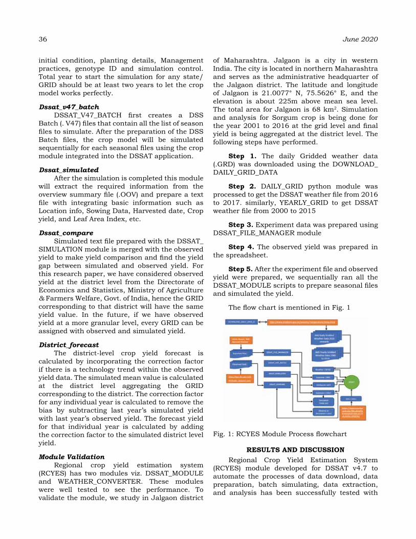
36 June 2020

initial condition, planting details, Management practices, genotype ID and simulation control. Total year to start the simulation for any state/GRID should be at least two years to let the crop model works perfectly.

Dssat_v47_batchDSSAT_V47_BATCH first creates a DSS

Batch (. V47) files that contain all the list of season files to simulate. After the preparation of the DSS Batch files, the crop model will be simulated sequentially for each seasonal files using the crop module integrated into the DSSAT application.

Dssat_simulatedAfter the simulation is completed this module

will extract the required information from the overview summary file (.OOV) and prepare a text file with integrating basic information such as Location info, Sowing Data, Harvested date, Crop yield, and Leaf Area Index, etc.

Dssat_compareSimulated text file prepared with the DSSAT_

SIMULATION module is merged with the observed yield to make yield comparison and find the yield gap between simulated and observed yield. For this research paper, we have considered observed yield at the district level from the Directorate of Economics and Statistics, Ministry of Agriculture & Farmers Welfare, Govt. of India, hence the GRID corresponding to that district will have the same yield value. In the future, if we have observed yield at a more granular level, every GRID can be assigned with observed and simulated yield.

District_forecastThe district-level crop yield forecast is

calculated by incorporating the correction factor if there is a technology trend within the observed yield data. The simulated mean value is calculated at the district level aggregating the GRID corresponding to the district. The correction factor for any individual year is calculated to remove the bias by subtracting last year’s simulated yield with last year’s observed yield. The forecast yield for that individual year is calculated by adding the correction factor to the simulated district level yield.

Module ValidationRegional crop yield estimation system

(RCYES) has two modules viz. DSSAT_MODULE and WEATHER_CONVERTER. These modules were well tested to see the performance. To validate the module, we study in Jalgaon district

of Maharashtra. Jalgaon is a city in western India. The city is located in northern Maharashtra and serves as the administrative headquarter of the Jalgaon district. The latitude and longitude of Jalgaon is 21.0077° N, 75.5626° E, and the elevation is about 225m above mean sea level. The total area for Jalgaon is 68 km2. Simulation and analysis for Sorgum crop is being done for the year 2001 to 2016 at the grid level and final yield is being aggregated at the district level. The following steps have performed.

Step 1. The daily Gridded weather data (.GRD) was downloaded using the DOWNLOAD_DAILY_GRID_DATA

Step 2. DAILY_GRID python module was processed to get the DSSAT weather file from 2016 to 2017. similarly, YEARLY_GRID to get DSSAT weather file from 2000 to 2015

Step 3. Experiment data was prepared using DSSAT_FILE_MANAGER module

Step 4. The observed yield was prepared in the spreadsheet.

Step 5. After the experiment file and observed yield were prepared, we sequentially ran all the DSSAT_MODULE scripts to prepare seasonal files and simulated the yield.

The flow chart is mentioned in Fig. 1

Fig. 1: RCYES Module Process flowchart

reSuLtS aNd dISCuSSIoNRegional Crop Yield Estimation System

(RCYES) module developed for DSSAT v4.7 to automate the processes of data download, data preparation, batch simulating, data extraction, and analysis has been successfully tested with

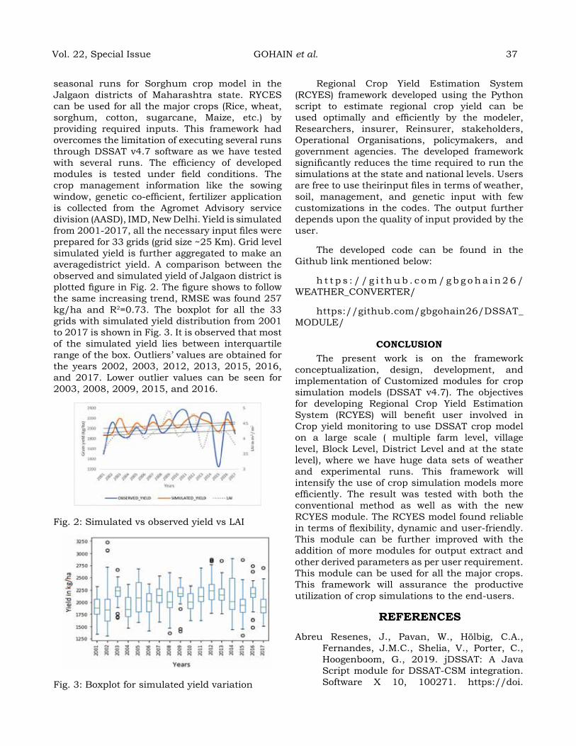
seasonal runs for Sorghum crop model in the Jalgaon districts of Maharashtra state. RYCES can be used for all the major crops (Rice, wheat, sorghum, cotton, sugarcane, Maize, etc.) by providing required inputs. This framework had overcomes the limitation of executing several runs through DSSAT v4.7 software as we have tested with several runs. The efficiency of developed modules is tested under field conditions. The crop management information like the sowing window, genetic co-efficient, fertilizer application is collected from the Agromet Advisory service division (AASD), IMD, New Delhi. Yield is simulated from 2001-2017, all the necessary input files were prepared for 33 grids (grid size ~25 Km). Grid level simulated yield is further aggregated to make an averagedistrict yield. A comparison between the observed and simulated yield of Jalgaon district is plotted figure in Fig. 2. The figure shows to follow the same increasing trend, RMSE was found 257 kg/ha and R2=0.73. The boxplot for all the 33 grids with simulated yield distribution from 2001 to 2017 is shown in Fig. 3. It is observed that most of the simulated yield lies between interquartile range of the box. Outliers’ values are obtained for the years 2002, 2003, 2012, 2013, 2015, 2016, and 2017. Lower outlier values can be seen for 2003, 2008, 2009, 2015, and 2016.

Fig. 2: Simulated vs observed yield vs LAI

Fig. 3: Boxplot for simulated yield variation

Regional Crop Yield Estimation System (RCYES) framework developed using the Python script to estimate regional crop yield can be used optimally and efficiently by the modeler, Researchers, insurer, Reinsurer, stakeholders, Operational Organisations, policymakers, and government agencies. The developed framework significantly reduces the time required to run the simulations at the state and national levels. Users are free to use theirinput files in terms of weather, soil, management, and genetic input with few customizations in the codes. The output further depends upon the quality of input provided by the user.

The developed code can be found in the Github link mentioned below:

h t t p s : / / g i t h u b . c o m / g b g o h a i n 2 6 /WEATHER_CONVERTER/

https://github.com/gbgohain26/DSSAT_MODULE/

CoNCLuSIoNThe present work is on the framework

conceptualization, design, development, and implementation of Customized modules for crop simulation models (DSSAT v4.7). The objectives for developing Regional Crop Yield Estimation System (RCYES) will benefit user involved in Crop yield monitoring to use DSSAT crop model on a large scale ( multiple farm level, village level, Block Level, District Level and at the state level), where we have huge data sets of weather and experimental runs. This framework will intensify the use of crop simulation models more efficiently. The result was tested with both the conventional method as well as with the new RCYES module. The RCYES model found reliable in terms of flexibility, dynamic and user-friendly. This module can be further improved with the addition of more modules for output extract and other derived parameters as per user requirement. This module can be used for all the major crops. This framework will assurance the productive utilization of crop simulations to the end-users.

reFereNCeS

Abreu Resenes, J., Pavan, W., Hölbig, C.A., Fernandes, J.M.C., Shelia, V., Porter, C., Hoogenboom, G., 2019. jDSSAT: A Java Script module for DSSAT-CSM integration. Software X 10, 100271. https://doi.

Vol. 22, Special Issue GOHAIN et al. 37

38 June 2020

org/10.1016/j.softx.2019.100271.A.K. Srivastava, M. Rajeevan and S. R. Kshirsagar,

Development of a high resolution daily gridded temperature data set (1969–2005) for the Indian region. Atmospheric Science Letter, https://doi.org/10.1002/asl.232

Alexandrov, V.A., Hoogenboom, G., 2001. The impact of climate variability and change on crop yield in Bulgaria. Agric. Forest Meteorol. 104, 315–327. Quemada, M., Cabrera, M.L., 1995. CERES-N model predictions of nitrogen mineralized from cover crop residues. Soil Sci. Soc. Am. J. 59, 1059–1065.

PATEL, A.K. NEMA, R.S. SINGH, M.K. YADAV, K.K. SINGH, S.K. SINGH, P.K. RAI, and S.M. SINGH, Assessment of climate change impact on wheat crop using MarkSim GCM in Varanasi, Uttar Pradesh, Journal of Agrometeorology 20 (3) :216-218 (September 2018)

D. S. PAI, LATHA SRIDHAR, M. RAJEEVAN*, O. P. SREEJITH, N. S. SATBHAI and B. MUKHOPADHYAY, Development of a new high spatial resolution (0.25° × 0.25°) long period (1901-2010) daily gridded rainfall data set over India and its comparison with existing data sets over the region. MAUSAM, 65, 1 551.501.777.

Fetcher, J., Allison, B.E., Sivakumar, M.V.K., van der Ploeg, R.R., Bley, J., 1991. An evaluation of the SWATRER and CERES-Millet models for southwest Niger. Soil Water Balance in the Sudano Sahelian Zone (Proceedings of the Niamey Workshop, February 1991). IAHS Publ. no. 199, 1991.

Gohain, G. B, and R. Bhatnagar. “Crop Yield Estimation Using Decision Trees and Random Forest Machine Learning Algorithms on Data from Terra (EOS AM-1) & Aqua (EOS PM-1) Satellite Data.” SpringerLink, Springer, Cham, 1 Jan. 1970, link.springer.com/chapter/10.1007/978-3-030-20212-5_6. Machine Learning and Data Mining in Aerospace Technology, springer

He, X., Peng, L., Sun, H., 2015. pyDSSAT documentation release 1.0. http://xiaoganghe.github.io/pyDSSAT/doc/_downloads/pyDSSATdoc.pdf (accessed February 12, 2020).

Hoogenboom, G., C.H. Porter, V. Shelia, K.J. Boote, U. Singh, J.W. White, L.A. Hunt, R. Ogoshi, J.I. Lizaso, J. Koo, S. Asseng, A. Singels, L.P.

Moreno, and J.W. Jones. 2019. Decision Support System for Agrotechnology Transfer (DSSAT) Version 4.7.5 (https://DSSAT.net). DSSAT Foundation, Gainesville, Florida, USA.

J. Chen, M. Li, W. Wang, Statistical uncertainty estimation using random forests and its application to drought forecast. Math. Probl. Eng. (2012)

Jones, J.W., G. Hoogenboom, C.H. Porter, K.J. Boote, W.D. Batchelor, L.A. Hunt, P.W. Wilkens, U. Singh, A.J. Gijsman, and J.T. Ritchie. 2003. DSSAT Cropping System Model. European Journal of Agronomy 18:235‐265.

Keating, B.A., Carberry, P.S., Hammer, G.L., Probert, M.E., Robertson, M.J., Holzworth, D., Huth, N.I., Hargreaves, J.N., Meinke, H., Hochman, Z., et al., 2003. An overview of apsim, a model designed for farming systems simulation. Eur. J. Agron. 18 (3–4), 267–288.

Koo, J., 2016. DSSAT listed as one of the greatest accomplishments of the UF-IFAS. https://dssat.net/2164 (accessed November 6, 2019).

M. Lal, K. K. Singh, L. S. Rathore, G. Srinivasan and S. A. Saseendran. 1998. Vulnerability of rice and wheat yields in NW-India to future changes in climate. Agricultural & Forest Metorology. 89, 101-114

S. A. Saseendran, K. K. Singh, L. S. Rathore, S. V. Singh and S. K. Sinha. 2000. Effects of climate change on rice production in the tropical humid climate of Kerala, India. Climatic Change, 44:495-514

S. Fukuda, W. Spreer, E. Yasunaga, K. Yuge, V. Sardsud, J. Müller, Random forests modelling for the estimation of mango (Mangiferaindica L. cv. chokanan) fruit yields under different irrigation regimes. Agric. Water Manag. 116, 142–150 (2013)

Singh, K.K., Baxla, A.K., Chattopadhyay, N., Balasubramanian, R., Singh, P.K., Rana, Mamta, Gohain, Ganesh Borpatra, Vishnoi, Lata and Singh, Priyanka (2017) Crop Yield forecasting under FASAL. FASAL Technical Report-2017. India Meteorological Department, New Delhi, 155p

Van Diepen, C.v., Wolf, J., Van Keulen, H., Rappoldt, C., 1989. WOFOST: a simulation model of crop production. Soil Use Manag. 5 (1), 16–24.

delineation of efficient Cropping Zone for onion over tamil Nadu

BavISh, S1*., geethaLaKShMI, v2., KoKILavaNI, S1., goWthaM, r1., BhuvaNeSWarI, K2., aNd raMaNathaN, SP1.1Agro Climate Research Centre, TNAU, Coimbatore – 641 003, India;

2Directorate of Crop Management, TNAU, Coimbatore – 641 003, India

aBStraCtOnion is one of the most important vegetable crops grown in India and cultivated under a broad range of climate. The spatial variability in climate and edaphic factors mainly regulate the distribution and productivity of the crops over the different regions and thus, area and yield potential of the crops widely vary from place to place. Delineation of efficient cropping zones contributes for identifying and developing the site-specific management approaches to increase the yield and area under the particular crop and meet out the demand of that crop. In the present investigation, Efficient Cropping Zones (ECZ) for small onion cultivation in Tamil Nadu were delineated at district scale by computing Relative Spread Index (RSI) and Relative Yield Index (RYI).The highest RSI was observed in Perambalur district while the Coimbatore district hold the first position in onion productivity with the highest RYI (155). In Tamil Nadu, 6, 14, 3 and 8 districts were classified under Most Efficient Cropping Zone (MECZ), Area Efficient Cropping Zone (AECZ), Yield Efficient Cropping Zone (YECZ) and Not Efficient Cropping Zone (NECZ), respectively. The identified districts of MECZ wereCoimbatore, Tiruppur, Nammakkal, Tirunelveli, Tiruchirapalli and Dindigul. The districts viz., Perambalur, Tutucorin and Virudhunagar were come under AECZ, could be brought under MECZ by adopting yield improvement technologies. The 14 districts viz., Erode, Ariyalur, Karur, Krishnagiri, Dharmapuri, Theni, Thanjavur, Vellore, Villupuram, Sivaganga, Cuddalore, Tiruvannamalai, Ramanathapuram and Salem, were classified under YECZ need extension activities to improve the area under Onion cultivation. It is suggested to promote other efficient crops in the eight NECZ districts viz., Pudukkottai, Madurai, Nagapattinam, Tiruvallur, The Nilgiris, Kancheepuram, Tiruvarur and Kanyakumari.

Keywords: Onion, Efficient Cropping Zone, Relative Spread Index and Relative Yield Index.

INtroduCtIoN

Onion (Allium cepa var. aggregatum L.), originated from Central Asia, is one of the most significant vegetables produced in India after potato (Mehta, 2017), consumed by all divisions of individuals as their utility as a therapeutic herb referenced even in Charaka Samhitha dated back to around 600 B.C. and also inSusrutha, Samhitha of third - fourth century A.D (Estes, 2000). Over the globe, Onion is cultivated in 5.3 million ha with a yearly production of 88.5 million tons representing per hectare productivity of 16.7 tons (Anon, 2017). The world Onion production increased from 35 million tons in 1980s to 90 million tons by 2011 (FAOSTAT, 2012) and further to 93 million tons during 2019 (Atlas big, 2019).Among the onion producing countries, next to China, India stands second in production with 22.4 million tons per annum from an area of 1.3 million hectare with a productivity of 17.1 tons per ha. During 2019, onion alone contributed INR 3742 crores through foreign exchange (Economic occasions Mar 02, 2020).

Onion production as well as onion price fluctuate heavily from time to time. For example, in 2018, mandis were flooded with onions due to thebumper harvest, and farmers were forced to either go for distress sales or abandoning their crop in the fields without harvesting as prices dropped (Murthy, 2019). In contrast, in 2019, due to weather vagaries that occurred in all three onion growing seasons, the area under onion was reduced and the supply got decreased by 25 per cent, leading to spike in onion price. Government of India has released an order on 29 September 2019 and banned onion exports to check a nationwide uproar over a shortfall in supply, sending ripples in the markets of neighboring Bangladesh, which relies heavily on Indian onions to balance its nearly one million tonnes of shortage in yearly supply.

The scope for the horizontal expansion of the cropped area in the future is limited and the crops adaptability to a particular region determines the productivity of the concerned crop. However, in most of the cases, the realized yield of crops is much lower than the achievable potential yield


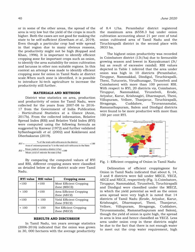
40 June 2020

or in some of the other areas, the spread of the area is very low but the yield of the crops is much higher. Both the cases are not good for making the state to be self-sufficient (Gowtham et al., 2019). Even though a particular crop had wide spread in that region due to many obvious reasons, the productivity might not be high (Koppad and Khan, 1996). It is important to identify efficient cropping zone for important crops such as onion, to identify the area suitability for onion cultivation and lacunas in other non suitable regions. In this context an attempt was made to identify efficient cropping zone for onion in Tamil Nadu at district scale.When such zone is identified, it is possible to introduce hi-tech agriculture to increase the productivity still further.

MaterIaLS aNd MethodSDistrict wise statistics on area, production

and productivity of onion for Tamil Nadu, were collected for the years from 2007-08 to 2016-17 from the Government of India Publication - Horticultural Statistics at a Glance (Anon, 2017b). From the collected information, Relative Spread Index (RSI) and Relative Yield Index (RYI) were computed using the following formula as suggested by Kanwar (1972) and further validated bySanbagavalli et al. (2002) and Kokilavani and Dheebakaran (2019).

By comparing the computed values of RYI and RSI, different cropping zones were classified as detailed below at the district scale over Tamil Nadu.

rYI value rSI value Cropping zone>100 >100 Most Efficient Cropping

Zone (MECZ) < 100 >100 Area Efficient Cropping

Zone (AECZ) >100 < 100 Yield Efficient Cropping

Zone (YECZ) < 100 < 100 Not Efficient Cropping

Zone (NECZ)

reSuLtS aNd dISCuSSIoN In Tamil Nadu, ten years average statistics

(2006-2016) indicated that the onion was grown in 30, 000 hectares with the average productivity

of 8.4 t/ha. Perambalur district registered the maximum area (6558.3 ha) under onion cultivation accounting about 21 per cent of total onion cultivated area of Tamil Nadu and the Tiruchirapalli district in the second place with 3833 ha.

The highest onion productivity was recorded in Coimbatore district (13t/ha) due to favourable growing season and lowest in Kanyakumari (3t/ha) as result of excessive rainfall. RSI values depicted in Table 1 inferred that the area under onion was high in 10 districts (Perambalur, Tiruppur, Nammakkal, Dindigul, Tiruchirapalli, Theni, Tutucorin, Virudhunagar, Tirunelveli and Coimbatore) with more than 100 percent RSI. With respect to RYI, 20 districts viz, Coimbatore, Tiruppur, Nammakkal, Tirunelveli, Erode, Ariyalur, Karur, Krishnagiri, Dharmapuri, Theni, Villupuram, Vellore, Thanjavur, Tiruchirapalli, Sivaganga, Cuddalore, Tiruvannamalai, Ramanathapuram, Salem and Dindigul districts were found to be more productive with more than 100 per cent RYI.

Fig. 1: Efficient cropping of Onion in Tamil Nadu

Delineation of efficient croppingzone for Onion in Tamil Nadu indicated that about 6, 14, 3 and 8 districts were fall under MECZ, YECZ, AECZ and NECZ, respectively (Fig. 1).Coimbatore, Tiruppur, Nammakkal, Tirunelveli, Tiruchirapalli and Dindigul were classified under the MECZ, in which the yield potential as well as the onion area spread were very high.It is noted that 14 districts of Tamil Nadu (Erode, Ariyalur, Karur, Krishnagiri, Dharmapuri, Theni, Thanjavur, Vellore, Villupuram, Sivaganga, Cuddalore, Tiruvannamalai, Ramanathapuram and Salem), though the yield of onion is quite high, the spread in area is less and hence classified as YECZ. Less area under onion crop in these districts might be due to the fact that there is not enough water to meet out the crop water requirement, high

production cost, higher susceptibility of onion crop to pest and diseases, high fluctuation in price as well as inadequate storage facilities.

In few of the districts of Tamil Nadu viz., Perambalur, Tutucorin and Virudhunagar, onion is cultivated in larger area, however the productivity is very low falling in to AECZ. More area under onion in these districts might be due to the farmer’s preference in taking up onion cultivation. However, the yield levels are low and might be due to improper selection of varieties, non-adoption of good management practices, unfavourable weather conditions including frequent changes in monsoon behaviours and low soil fertility. In these districts, there is lot of scope to improve the productivity by providing capacity building on good crop management and yield

improving technologies.

In Tamil Nadu, the eight districts viz., Pudukkottai, Madurai, Nagapattinam, Tiruvallur, The Nilgiris, Kancheepuram, Tiruvarur and Kanyakumari were categorised under the Non Efficient Cropping Zone (NECZ) for onion (Table 1). Out of 8 districts of NECZ, Madurai alone had RSI value of 57.9 per cent rest of the seven districts had almost no area under onion with very low RYI values. This might be mainly due to the unfavourable weather conditions that prevail in these districts for onion cultivation. All these seven districts are close to the ocean and receive high intensity rainfall and the water stagnation affects the growth and development of onion.

When the analysis was made at agroclimatic zone level, it could clearly be noted that the

Table 1: Efficient Onion cropping zone over Tamil Nadu (2001-2015)

district onion area (ha)

Yield (t/ha)

Cultivable area (ha)

% onion area to to-tal cultivable area

rSI rYI Zone Clas-sification

Kancheepuram 1.0 4543 274230.3 0.0004 0.08 54 NECZTiruvallur 1.1 5304 67153.6 0.0017 0.39 63 NECZCuddalore 67.5 9243 434433.2 0.0155 3.58 109 YECZVillupuram 197.5 9357 248639.4 0.0794 18.30 111 YECZVellore 40.4 9414 345854.9 0.0117 2.69 111 YECZTiruvannamalai 72.5 9144 234380.8 0.0309 7.13 108 YECZSalem 844.4 8592 377797.0 0.2235 51.50 102 YECZNammakkal 2374.3 11493 101945.8 2.3290 536.61 136 MECZDharmapuri 308.5 9466 420333.4 0.0734 16.91 112 YECZKrishnagiri 109.8 9480 71787.2 0.1530 35.25 112 YECZCoimbatore 1831.9 13096 403520.8 0.4540 104.60 155 MECZTiruppur 2929.3 12339 56557.1 5.1793 1193.33 146 MECZErode 1725.7 10639 407199.7 0.4238 97.65 126 YECZTiruchirapalli 3833.9 9264 434288.5 0.8828 203.40 110 MECZKarur 192.1 9514 56156.9 0.3420 78.80 112 YECZPerambalur 6558.3 8044 121856.6 5.3820 1240.01 95 AECZAriyalur 47.4 10053 22987.0 0.2063 47.54 119 YECZPudukkottai 4.3 8233 204000.2 0.0021 0.49 97 NECZThanjavur 22.5 9418 329048.5 0.0068 1.57 111 YECZTiruvarur 0.2 4494 78529.0 0.0003 0.06 53 NECZNagapattinam 9.5 6102 126160.3 0.0075 1.73 72 NECZMadurai 805.5 7957 320046.8 0.2517 57.99 94 NECZTheni 518.4 9427 61926.5 0.8371 192.87 111 YECZDindigul 3068.7 8416 232844.9 1.3179 303.65 100 MECZRamanathapuram 120.9 9022 313013.0 0.0386 8.90 107 YECZVirudhunagar 1254.9 6350 168417.4 0.7451 171.67 75 AECZSivaganga 25.3 9301 122550.8 0.0206 4.75 110 YECZTirunelveli 1669.1 11273 263334.5 0.6338 146.04 133 MECZTutucorin 1427.7 5369 184987.3 0.7718 177.82 63 AECZThe Nilgiris 1.2 4983 81788.7 0.0015 0.34 59 NECZKanyakumari 0.1 2829 82741.5 0.0002 0.04 33 NECZ

Vol. 22, Special Issue BAVISH et al. 41

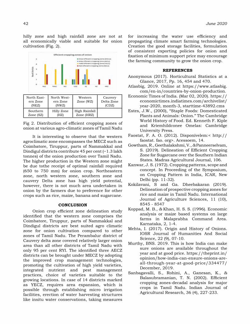
42 June 2020

hilly zone and high rainfall zone are not at all economically viable and suitable for onion cultivation (Fig. 2).

North East-ern Zone

(NEZ)

North West-ern Zone

(NWZ)

Western Zone (WZ)

Cauvery Delta Zone

(CDZ)

Southern Zone (SZ)

Hilly Zone (HZ)

High Rainfall Zone (HRZ)

Fig 2. Distribution of efficient cropping zones of onion at various agro-climatic zones of Tamil Nadu

It is interesting to observe that the western agroclimatic zone encompasses the MECZ such as Coimbatore, Tiruppur, parts of Nammakkal and Dindigul districts contribute 45 per cent (~1.3 lakh tonnes) of the onion production over Tamil Nadu. The higher production in the Western zone might be due tothe receipt of optimal rainfall required (650 to 750 mm) for onion crop. Northeastern zone, north western zone, southern zone and cauvery Delta zone has high yield potential, however, there is not much area undertaken in onion by the farmers due to preference for other crops such as rice, maize, banana and sugarcane.

CoNCLuSIoNOnion crop efficient zone delineation study

identified that the western zone comprises the Coimbatore, Tiruppur, parts of Nammakkal and Dindigul districts are best suited agro climatic zone for onion cultivation compared to other zones of Tamil Nadu. The Perambalur district of Cauvery delta zone covered relatively larger onion area than all other districts of Tamil Nadu with only 95 per cent RYI. The identified three AECZ districts can be brought under MECZ by adopting the improved crop management technologies, promoting the cultivation of high yield varieties, integrated nutrient and pest management practices, choice of varieties suitable to the growing locations. In case of 14 districts marked as YECZ, requires area expansion, which is possible through establishing micro irrigation facilities, erection of water harvesting structures like insitu water conservations, taking measures

for increasing the water use efficiency and propagating climate smart farming technologies. Creation the good storage facilities, formulation of consistent exporting policies for onion and fixation of minimum support price may encourage the farming community to grow the onion crop.

reFereNCeSAnonymous (2017). Horticultural Statistics at a

Glance, 2017, Pp. 16, 454 and 470. Atlasbig, 2019. Online at https://www.atlasbig.

com/en-in/countries-by-onion-production.Economic Times of India. (Mar 02, 2020). https://

economictimes.indiatimes.com/archivelist/year-2020, month-3, starttime-43892.cms

Estes, J.W., (2000), “Staple Foods: Domesticated Plants and Animals: Onion.” The Cambridge World History of Food. Ed. Kenneth F. Kiple and Kriemhildconee Omelas: Cambridge University Press.

Faostat, F. A. O. (2012). Disponívelem:< http://faostat. fao. org>. Acessoem, 14.

Gowtham, R., Geethalakshmi, V., & Panneerselvam, S. (2019). Delineation of Efficient Cropping Zone for Sugarcane over the Southern Indian States. Madras Agricultural Journal, 106.

Kanwar, J. S. (1972). Cropping patterns, scope and concept. In Proceeding of the Symposium, on Cropping Pattern in India, ICAR, New Delhi (pp. 11-32).

Kokilavani, S and Ga. Dheebakaran (2019). Delineation of prospective cropping zones for rice and maize in Tamil Nadu. International Journal of Agriculture Sciences, 11 (10), 8545 - 8547

Koppad, M. B., & Khan, H. S. S. (1996). Economic analysis or maize based systems on large farms in Malaprabha Command Area. Karnataka, 2, 1-4.

Mehta, I. (2017). Origin and History of Onions. IOSR Journal of Humanities And Social Science, 22 (9), 07-10.

Murthy, BNS. 2019. This is how India can make sure onions are available throughout the year and at good price. https://theprint.in/opinion/how-india-can-ensure-onions-are-all-through-year-at-good-price/334477/December, 2019.

Sanbagavalli, S., Rohini, A., Ganesan, K., & Balasubramanian, T. N. (2002). Efficient cropping zones-decadal analysis for major crops in Tamil Nadu. Indian Journal of Agricultural Research, 36 (4), 227-233.

analysis of drought in the Maharashtra by using the Standardized Precipitation Index

K. K. daKhore1, a. KaruNaKar2, J. d. Jadhav3 Y.e KadaM4, d. P.WaSKar5 aNd P. vIJaYa KuMar6

1Agro meteorologist, AICRP on Agrometeorology, VNMKV, Parbhani2Associate Professor, GKMS, Dr. PDKV, Akola

3HOD, CAFT, MPKV, Pune4Senior research fellow, FASAL, VNMKV, Parbhani

5Director of research, VNMKV, Parbhani6Project Coordinator, AICRP on Agrometeorology, CRIDA, Hyderabad

correspondence email: [email protected]

aBStraCtDrought is a one of the most destructive climate-related hazards, it is in general unstated as a prolonged deficiency of precipitation. Drought features are thus recognized as important factors in water resources planning and management. The purpose of this study is to detect the changes in drought frequency, persistence, and severity in the Maharashtra. Drought probabilities for different talukas of Maharashtra based on SPI methodology was computed for three time scales (Annual — 12 months scale, Southwest monsoon — 4 months scale, and Post monsoon — 3 months scale) for 326 talukas for which daily rainfall data for 30 years or more was used. The main benefit of the application of this index is its versatility, only rainfall data are required to deliver five major dimensions of a drought: duration, intensity, severity, magnitude, and frequency. It is interesting to note that highest probability (89%) is observed in Shirur Anantpal and Udgir taluka of Latur district followed by Loha taluka in Nanded district and Kamptee taluka in Nagpur (89%). Though they are situated in a semi-arid climatic region, near normal conditions are being expected over these talukas. In talukas from coastal Kokan region where annual rainfall is higher, the occurrence of near normal condition is less. Probability of 70 and above has been considered generally as a benchmark for making decisions on agricultural operations, and this is observed in 128 talukas out of 328 talukas across the state for near normal condition. The Lowest probability for normal conditions is noted in Murtijapur talukas in Akola district (50%) followed by Sangrampur in Buldhana district (53%) and Digras in Yavatmal district (54%). The Highest probability of occurrence for moderately dry condition is seen in Manora in Washim district and Parseoni Nagpur district (21%) followed by 20 percent probability in Ralegaon in Yavatmal district and Chopda in Jalgaon district. It can be inferred that 2 out of 10 years moderate dry conditions can be expected in the above talukas. The probability of occurrence of severe and extremely dry conditions is almost nil in 86 and 139 talukas, respectively. The Highest probability (13%) under severe dry category has been noted in 2 talukas and extremely dry conditions may prevail with a 21% probability in Mauda taluka of Nagpur district.

Keywords : Drought, Maharashtra, Precipitation, Standardized Precipitation Index (SPI).

INtroduCtIoN

Drought is fused natural hazard, which has a lethargic onset and is defined by the severe water scarcity. It is described in many ways, depending on its impact and varying characteristics. The prolonged low rainfall marks the onset of meteorological drought, which is followed by hydrological drought as a decline in the water surface and ground water levels (Hisdal and Tallaksen, 2003), which has a straight effect on the agricultural crops resulting in agricultural drought (Mishra and Singh, 2010). Therefore, depending on the impact, which drought has on

diverse sectors, it is classified into Meteorological, Hydrological, and Agricultural drought. The effect of drought can be seen universal on the livelihood, environment, economy, and overall human safety. Being the most important environmental problems affecting our earth, drought has been ranked as the ‘third most costly geophysical phenomena’ (Oladipo, 1993). Of these, the meteorological drought signifies the paucity of rainfall over a region for a considerable period. Climatic conditions / factors like high temperature, and a high wind can only worsen its intensity. It should also be noted that a detailed analysis of drought also requires understanding of


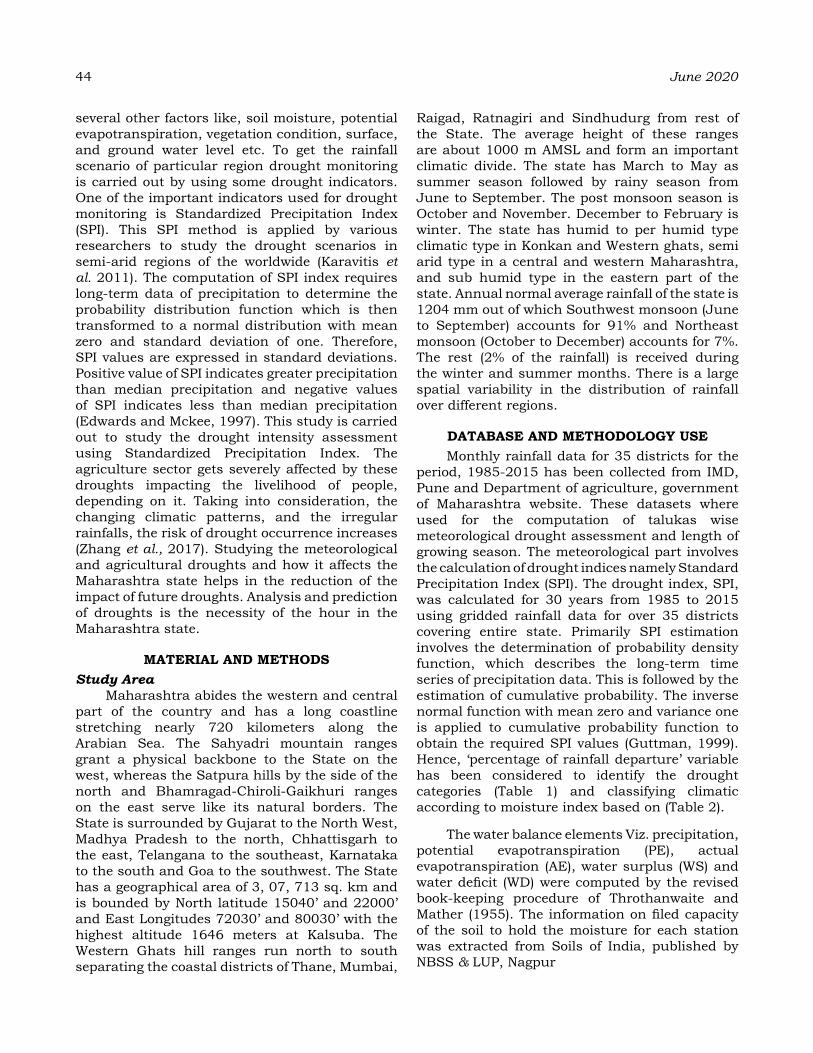
44 June 2020

several other factors like, soil moisture, potential evapotranspiration, vegetation condition, surface, and ground water level etc. To get the rainfall scenario of particular region drought monitoring is carried out by using some drought indicators. One of the important indicators used for drought monitoring is Standardized Precipitation Index (SPI). This SPI method is applied by various researchers to study the drought scenarios in semi-arid regions of the worldwide (Karavitis et al. 2011). The computation of SPI index requires long-term data of precipitation to determine the probability distribution function which is then transformed to a normal distribution with mean zero and standard deviation of one. Therefore, SPI values are expressed in standard deviations. Positive value of SPI indicates greater precipitation than median precipitation and negative values of SPI indicates less than median precipitation (Edwards and Mckee, 1997). This study is carried out to study the drought intensity assessment using Standardized Precipitation Index. The agriculture sector gets severely affected by these droughts impacting the livelihood of people, depending on it. Taking into consideration, the changing climatic patterns, and the irregular rainfalls, the risk of drought occurrence increases (Zhang et al., 2017). Studying the meteorological and agricultural droughts and how it affects the Maharashtra state helps in the reduction of the impact of future droughts. Analysis and prediction of droughts is the necessity of the hour in the Maharashtra state.

MaterIaL aNd MethodS Study Area

Maharashtra abides the western and central part of the country and has a long coastline stretching nearly 720 kilometers along the Arabian Sea. The Sahyadri mountain ranges grant a physical backbone to the State on the west, whereas the Satpura hills by the side of the north and Bhamragad-Chiroli-Gaikhuri ranges on the east serve like its natural borders. The State is surrounded by Gujarat to the North West, Madhya Pradesh to the north, Chhattisgarh to the east, Telangana to the southeast, Karnataka to the south and Goa to the southwest. The State has a geographical area of 3, 07, 713 sq. km and is bounded by North latitude 15040’ and 22000’ and East Longitudes 72030’ and 80030’ with the highest altitude 1646 meters at Kalsuba. The Western Ghats hill ranges run north to south separating the coastal districts of Thane, Mumbai,

Raigad, Ratnagiri and Sindhudurg from rest of the State. The average height of these ranges are about 1000 m AMSL and form an important climatic divide. The state has March to May as summer season followed by rainy season from June to September. The post monsoon season is October and November. December to February is winter. The state has humid to per humid type climatic type in Konkan and Western ghats, semi arid type in a central and western Maharashtra, and sub humid type in the eastern part of the state. Annual normal average rainfall of the state is 1204 mm out of which Southwest monsoon (June to September) accounts for 91% and Northeast monsoon (October to December) accounts for 7%. The rest (2% of the rainfall) is received during the winter and summer months. There is a large spatial variability in the distribution of rainfall over different regions.

dataBaSe aNd MethodoLogY uSeMonthly rainfall data for 35 districts for the

period, 1985-2015 has been collected from IMD, Pune and Department of agriculture, government of Maharashtra website. These datasets where used for the computation of talukas wise meteorological drought assessment and length of growing season. The meteorological part involves the calculation of drought indices namely Standard Precipitation Index (SPI). The drought index, SPI, was calculated for 30 years from 1985 to 2015 using gridded rainfall data for over 35 districts covering entire state. Primarily SPI estimation involves the determination of probability density function, which describes the long-term time series of precipitation data. This is followed by the estimation of cumulative probability. The inverse normal function with mean zero and variance one is applied to cumulative probability function to obtain the required SPI values (Guttman, 1999). Hence, ‘percentage of rainfall departure’ variable has been considered to identify the drought categories (Table 1) and classifying climatic according to moisture index based on (Table 2).

The water balance elements Viz. precipitation, potential evapotranspiration (PE), actual evapotranspiration (AE), water surplus (WS) and water deficit (WD) were computed by the revised book-keeping procedure of Throthanwaite and Mather (1955). The information on filed capacity of the soil to hold the moisture for each station was extracted from Soils of India, published by NBSS & LUP, Nagpur

The water balance indices such as humidity index (Ih) and aridity index (Ia) and moisture index (Im) were calculated using formulae:

1. Humidity index Ih = WS/PE X 100

2. Aridity index Ia = WD/PE X 100

3. Moisture index Im = Ih-Ia

Based on Aridity index and Humidity index, the moisture index was calculated. Using moisture index (Table 2), talukas have been classified in to different climatic types.

Table 1: Categorization of climates based on Standard Precipitation Index (SPI)

SPI range CategoryMore than +2.0 Severely wet1.5 to 1.99 Very wet1.0 to 1.49 Moderately wet-0.99 to +0.99 Near normal-1.0 to -1.49 Moderately dry-1.5 to -1.99 Severely dryLess than -2.0 Extremely dry

Table 2: Classification of climates according to moisture index (%) Climate type (Symbol)

Above 100 Pre-humid (A) 100-80 Humid (B4) 80-60 Humid (B3) 60-40 Humid (B2) 40-20 Humid (B1) 0-20 Moist Sub-humid (C2) 0 to -33.3 Dry Sub-humid (C1) -33.3 to -66.7 Semi-arid (D) Less than -66.7 Arid (E)

reSuLt aNd dISCuSSIoNAverage annual rainfall for Maharashtra

The mean annual and seasonal rainfall for the state (except Mumbai district) is furnished spatial distribution in (Fig. 1). The mean annual rainfall of Maharashta is 1204 ± 358 mm with a coefficient of variation of 36% (Fig. 2). Maharashtra is divided into four meteorological sub-divisions viz., Konkan, Madhya Maharashtra, Marathwada and Vidarbha. Annual rainfall is the highest over coastal Konkan region (3039 mm), lowest over Madhya Maharashtra (927 mm), Marathwada region (630 mm) while it is intermediary over the Vidarbha region (1039 mm). There is a large

variability in rainfall across the districts in Konkan region with Ratnagiri topping the list (3618 mm) followed by Sindhudurg (3292 mm) and Raigad (3082 mm). In Madhya Maharashtra region, Kolhapur receives the highest rainfall (1894 mm) followed by Satara (1389 mm) and Nashik (1062 mm). While in Marathwada region Hingoli receives the highest rainfall (737 mm) and Parbhani (649 mm). The rainfall in Vidarbha region is found to be higest in Gadchiroli (1479 mm), followed by Gondia (1353 mm), Bhandara (1241 mm), Chandrapur (1198 mm), and Nagpur (1043 mm). The Lowest rainfall was noticed in Ahemadnagar district (547 mm), Jalana (575 mm) and Osmanabad (598 mm) in the state. This is closely followed by Beed (602 mm), Dhule (607 mm), Latur (616 mm), Sangali (617 mm), Solapur (624 mm), Aurangabad (619 mm), Nanded (645 mm), and Parbhani (649 mm). The annual rainfall is highly variable in Nanded district followed by Latur and Parbhani districts. The Least variability has been noticed in Palghar and Ratnagiri districts.

Fig. 1. Annual rain (mm) over Maharashtra

Fig. 2. Spatial variability (CV%) of annual rain in Maharashtra

Vol. 22, Special Issue DAKHORE et al. 45

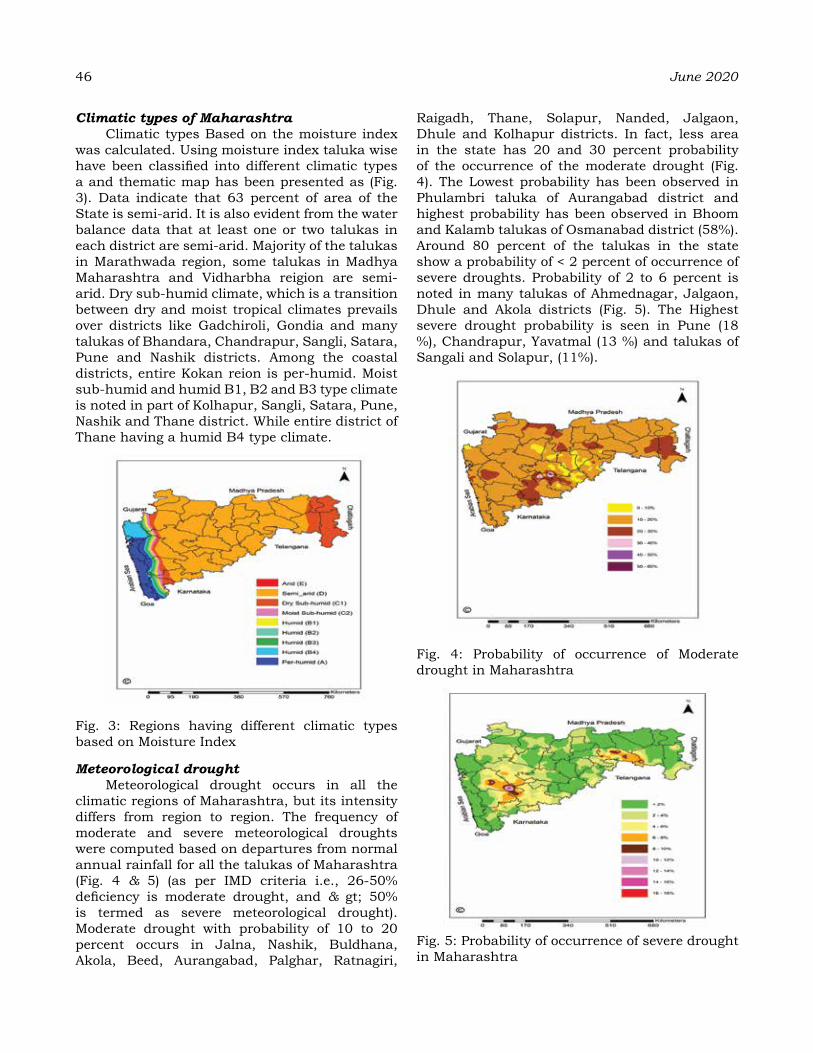
46 June 2020

Climatic types of MaharashtraClimatic types Based on the moisture index

was calculated. Using moisture index taluka wise have been classified into different climatic types a and thematic map has been presented as (Fig. 3). Data indicate that 63 percent of area of the State is semi-arid. It is also evident from the water balance data that at least one or two talukas in each district are semi-arid. Majority of the talukas in Marathwada region, some talukas in Madhya Maharashtra and Vidharbha reigion are semi-arid. Dry sub-humid climate, which is a transition between dry and moist tropical climates prevails over districts like Gadchiroli, Gondia and many talukas of Bhandara, Chandrapur, Sangli, Satara, Pune and Nashik districts. Among the coastal districts, entire Kokan reion is per-humid. Moist sub-humid and humid B1, B2 and B3 type climate is noted in part of Kolhapur, Sangli, Satara, Pune, Nashik and Thane district. While entire district of Thane having a humid B4 type climate.

Fig. 3: Regions having different climatic types based on Moisture Index

Meteorological droughtMeteorological drought occurs in all the

climatic regions of Maharashtra, but its intensity differs from region to region. The frequency of moderate and severe meteorological droughts were computed based on departures from normal annual rainfall for all the talukas of Maharashtra (Fig. 4 & 5) (as per IMD criteria i.e., 26-50% deficiency is moderate drought, and & gt; 50% is termed as severe meteorological drought). Moderate drought with probability of 10 to 20 percent occurs in Jalna, Nashik, Buldhana, Akola, Beed, Aurangabad, Palghar, Ratnagiri,

Raigadh, Thane, Solapur, Nanded, Jalgaon, Dhule and Kolhapur districts. In fact, less area in the state has 20 and 30 percent probability of the occurrence of the moderate drought (Fig. 4). The Lowest probability has been observed in Phulambri taluka of Aurangabad district and highest probability has been observed in Bhoom and Kalamb talukas of Osmanabad district (58%). Around 80 percent of the talukas in the state show a probability of < 2 percent of occurrence of severe droughts. Probability of 2 to 6 percent is noted in many talukas of Ahmednagar, Jalgaon, Dhule and Akola districts (Fig. 5). The Highest severe drought probability is seen in Pune (18 %), Chandrapur, Yavatmal (13 %) and talukas of Sangali and Solapur, (11%).

Fig. 4: Probability of occurrence of Moderate drought in Maharashtra

Fig. 5: Probability of occurrence of severe drought in Maharashtra

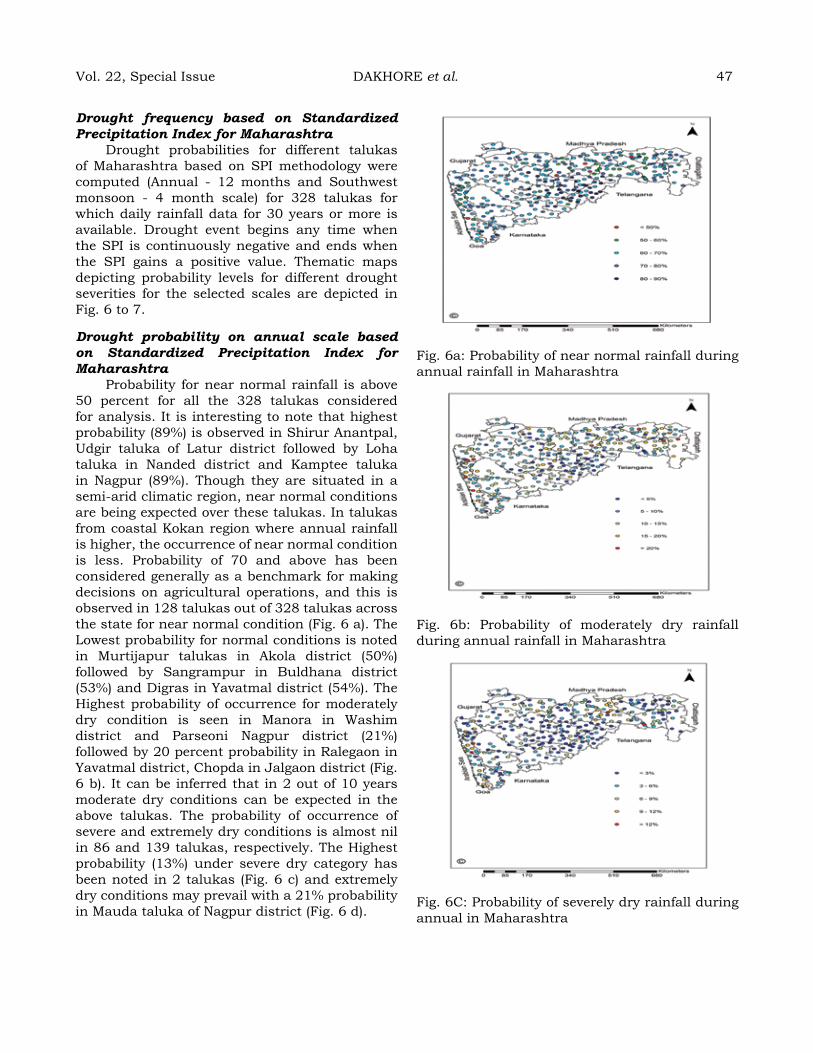
Drought frequency based on Standardized Precipitation Index for Maharashtra

Drought probabilities for different talukas of Maharashtra based on SPI methodology were computed (Annual - 12 months and Southwest monsoon - 4 month scale) for 328 talukas for which daily rainfall data for 30 years or more is available. Drought event begins any time when the SPI is continuously negative and ends when the SPI gains a positive value. Thematic maps depicting probability levels for different drought severities for the selected scales are depicted in Fig. 6 to 7.

Drought probability on annual scale based on Standardized Precipitation Index for Maharashtra

Probability for near normal rainfall is above 50 percent for all the 328 talukas considered for analysis. It is interesting to note that highest probability (89%) is observed in Shirur Anantpal, Udgir taluka of Latur district followed by Loha taluka in Nanded district and Kamptee taluka in Nagpur (89%). Though they are situated in a semi-arid climatic region, near normal conditions are being expected over these talukas. In talukas from coastal Kokan region where annual rainfall is higher, the occurrence of near normal condition is less. Probability of 70 and above has been considered generally as a benchmark for making decisions on agricultural operations, and this is observed in 128 talukas out of 328 talukas across the state for near normal condition (Fig. 6 a). The Lowest probability for normal conditions is noted in Murtijapur talukas in Akola district (50%) followed by Sangrampur in Buldhana district (53%) and Digras in Yavatmal district (54%). The Highest probability of occurrence for moderately dry condition is seen in Manora in Washim district and Parseoni Nagpur district (21%) followed by 20 percent probability in Ralegaon in Yavatmal district, Chopda in Jalgaon district (Fig. 6 b). It can be inferred that in 2 out of 10 years moderate dry conditions can be expected in the above talukas. The probability of occurrence of severe and extremely dry conditions is almost nil in 86 and 139 talukas, respectively. The Highest probability (13%) under severe dry category has been noted in 2 talukas (Fig. 6 c) and extremely dry conditions may prevail with a 21% probability in Mauda taluka of Nagpur district (Fig. 6 d).

Fig. 6a: Probability of near normal rainfall during annual rainfall in Maharashtra

Fig. 6b: Probability of moderately dry rainfall during annual rainfall in Maharashtra

Fig. 6C: Probability of severely dry rainfall during annual in Maharashtra


48 June 2020

Fig. 6d: Probability of extremely dry rainfall during annual in M Maharashtra

Drought probability during Southwest monsoon season based on Standardized Precipitation Index for Maharashtra

Probability for near normal condition during Southwest monsoon is above 50 percent for all 328 talukas. Probability of 70% and above for near normal conditions has been noted in nearly all talukas of Maharashtra (323 out of 328). However, the highest probability is observed in Kamptee taluka (95%) in Nagpur district followed by Loha in Nanded district (83%) Jalkot in Latur district (81%) and Kagal in Kolhapur district (80%). The Lowest probability of 51 percent in Sindkhed Raja (Buldhana district) and Mauda (Nagpur) talukas has been recorded (Fig. 7 a). In the case of moderately dry category, the highest probability of 28% and above noted in two talukas viz., Sindkhed Raja, Buldhana (32%) and Jivati (32%), Chandrapur district (Fig. 7 b). Very low probability for moderately dry condition to occur has been observed in Bhokardan (Jalana district), Deglur (Nanded district), Shrigonda (Ahemadnagar district), Mangalwedha (Solapur district) and Wani (Yavatmal district) talukas. Like-wise, probability for severely and extremely dry condition to occur has been noted in 248 and 178 talukas, respectively (Fig. 7 c). However, probability of occurrence of severely dry conditions is highest (16%) in Lakhni and Karanja talukas in Bhandara and Washim district respectively. While the Lonar talukas of Buldhana district the probability of extremely dry condition is highest (26%) in Kalmeshwar, Kuhi, Katol and Mauda talukas of Nagpur district (16%) (Fig. 7 d).

Fig. 7a: Probability of near normal rainfall during southwest monsoon in Maharashtra

Fig. 7b: Probability of moderately dry rainfall during southwest monsoon in Maharashtra

Fig. 7c: Probability of severely dry rainfall during southwest monsoon in Maharashtra

Fig. 7d: Probability of extremely dry rainfall during Southwest monsoon in Maharashtra

Length of growing period (LGP) The onset of monsoon determines the start of

growing season but the soil type as an important role to play on the feasibility of the sowing of crops due to differences in depth of wetting by rainfall and workability of soil. Therefore, the start of growing season in each talukas is computed and presented in (Fig. 8) for four soil water holding capacities (50, 100, 150, 200 and 250 mm). The range of LGP 18 to 21 weeks for 50 mm water holding capacity (WHC), similarly for 20 to 25 weeks in 100 mm WHC, 22 to 29 weeks for 150 mm WHC, 23 to 30 weeks for 200 mm WHC and 25 to 32 weeks for 200 mm WHC.

Fig. 8a: Commencement of growing season (SMW) for soils having water holding 50 mm in Maharashtra

Fig. 8b: Commencement of growing season (SMW) for soils having water holding 100 mm in Maharashtra

Fig. 8c: Commencement of growing season (SMW) for soils having water holding 150 mm in Maharashtra

Fig. 8d: Commencement of growing season (SMW) for soils having water holding 200 mm in Maharashtra


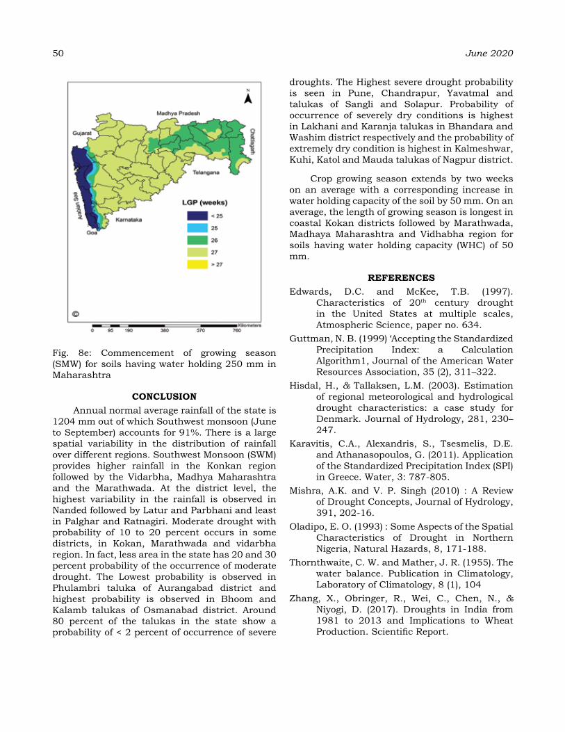
50 June 2020

Fig. 8e: Commencement of growing season (SMW) for soils having water holding 250 mm in Maharashtra

CoNCLuSIoNAnnual normal average rainfall of the state is

1204 mm out of which Southwest monsoon (June to September) accounts for 91%. There is a large spatial variability in the distribution of rainfall over different regions. Southwest Monsoon (SWM) provides higher rainfall in the Konkan region followed by the Vidarbha, Madhya Maharashtra and the Marathwada. At the district level, the highest variability in the rainfall is observed in Nanded followed by Latur and Parbhani and least in Palghar and Ratnagiri. Moderate drought with probability of 10 to 20 percent occurs in some districts, in Kokan, Marathwada and vidarbha region. In fact, less area in the state has 20 and 30 percent probability of the occurrence of moderate drought. The Lowest probability is observed in Phulambri taluka of Aurangabad district and highest probability is observed in Bhoom and Kalamb talukas of Osmanabad district. Around 80 percent of the talukas in the state show a probability of < 2 percent of occurrence of severe

droughts. The Highest severe drought probability is seen in Pune, Chandrapur, Yavatmal and talukas of Sangli and Solapur. Probability of occurrence of severely dry conditions is highest in Lakhani and Karanja talukas in Bhandara and Washim district respectively and the probability of extremely dry condition is highest in Kalmeshwar, Kuhi, Katol and Mauda talukas of Nagpur district.

Crop growing season extends by two weeks on an average with a corresponding increase in water holding capacity of the soil by 50 mm. On an average, the length of growing season is longest in coastal Kokan districts followed by Marathwada, Madhaya Maharashtra and Vidhabha region for soils having water holding capacity (WHC) of 50 mm.

reFereNCeS Edwards, D.C. and McKee, T.B. (1997).

Characteristics of 20th century drought in the United States at multiple scales, Atmospheric Science, paper no. 634.

Guttman, N. B. (1999) ‘Accepting the Standardized Precipitation Index: a Calculation Algorithm1, Journal of the American Water Resources Association, 35 (2), 311–322.

Hisdal, H., & Tallaksen, L.M. (2003). Estimation of regional meteorological and hydrological drought characteristics: a case study for Denmark. Journal of Hydrology, 281, 230–247.

Karavitis, C.A., Alexandris, S., Tsesmelis, D.E. and Athanasopoulos, G. (2011). Application of the Standardized Precipitation Index (SPI) in Greece. Water, 3: 787-805.

Mishra, A.K. and V. P. Singh (2010) : A Review of Drought Concepts, Journal of Hydrology, 391, 202-16.

Oladipo, E. O. (1993) : Some Aspects of the Spatial Characteristics of Drought in Northern Nigeria, Natural Hazards, 8, 171-188.

Thornthwaite, C. W. and Mather, J. R. (1955). The water balance. Publication in Climatology, Laboratory of Climatology, 8 (1), 104

Zhang, X., Obringer, R., Wei, C., Chen, N., & Niyogi, D. (2017). Droughts in India from 1981 to 2013 and Implications to Wheat Production. Scientific Report.

“assessment of rice (Oryza sativa L.) productivity under different climate change scenarios”

JaStI veNKata SatISh aNd B. aJIthKuMarDepartment of Agricultural Meteorology, College of Horticulture, KAU, Thrissur

E-mail : [email protected]

aBStraCtAssessment of rice (Oryza sativa L.) productivity under different climate change scenarios were carried out during kharif season 2016 to determine the crop weather relationship, validation of CERES-Rice model for the varieties of Jyothi and Kanchana and to project the future changes of rice yield. The research was carried at Agriculture Research Station, Mannuthy, Thrissur, Kerala. Split plot design was taken on with five different dates of planting viz., 5th June, 20th June, 5th July, 20th July and 5th August as the main plots and two varieties viz., Jyothi and Kanchana as the sub plot treatments in four replications. The model output revealed that the data of simulated yield was well compatible with observed data. Analysis of yield and growth phases of rice under different climate change scenarios of RCP 4.5 and 8.5 for the periods 2050s and 2080s showed that the days required to panicle initiation, anthesis and physiological maturity decreases for each of the five different dates of planting. This is assumabily because of increase in maximum and minimum temperatures in the future scenarios. The predicted rice yield for the 5th June and 20th June plantings during 2050s and 2080s revealed lower yield whereas increase in yield was observed on 5th July to 5th August plantings when compared with the yield of 2016. This increase in yield is probably due to combined effect of escalated CO2 (538 and 936 ppm) and solar radiation during the panicle initiation, anthesis and physiological maturity for the later plantings.

Keywords: Climate change, RCPs, Rice yields and Simulation modelling

INtroduCtIoN

Climate change has been depicted as a major threat to future agricultural area and production. World agriculture faces overwhelming challenges to meet the rising demands for food, energy, and other agricultural products, and this coupled with increasing population and dwindling natural resources made it opaque to understand the consequences of climate change on the productivity of essential crop species. Numerous estimates for the impending decade projects that continuous rise of anthropogenic forcing leads to increase in Green House Gas (GHG) concentrations, which alters the regional temperatures and precipitation patterns, also contributing the higher risk of climate irregularity and extreme weather events (IPCC, 2013).Climate predictions of central Asia shows that by the end of twenty first century, temperatures are expected to rise by 3-40C and atmospheric CO2 concentrations could raise up to 485-1000 ppm. Under these scenarios, yields of the crops are expected to decline about 30 percent even though direct positive physiological effects of elevated CO2 are considered (Parry et al., 2007). Due to complex interactions between crop and climatic variables, it is challenging task

to project the change in climate over a region and its impact on any cropping system (Lobell et al., 2011). Therefore, increasing efforts to investigate the influence of climate change on agriculture are going on different spatial scales around the globe and also in India (Srivastava et al., 2010; Soora et al., 2013).

According to FAOSTAT (2015), India is contributing about 20 percent of total rice production of the world after China. Since rice is a primary food crop of India, it is essential to identify the impact of change in climate on rice yield to escalate the country’s rice production. Rice production in India varies year to year owing to annual rainfall variability. Severe drought during the year 2009-10 and 2011-12 results in decline of rice production by 10.1 and 16.8 percent in the country. This annual variation shows that countries rice production depends on the monsoon variability (Soora et al., 2013). Thus, investigation of impacts of climate change on agriculture are essential in order to avoid negative impacts on global and national food security.

In this contemporary world, application of the crop yield simulation systems approach to climate change adaptation and mitigation


52 June 2020

initiatives has been gaining popularity. This is because of increasing availability of information on the processes that are affected by changing climate, thus helping us to devise possible adaptation measures. Since all the crop models are limited limitations of real system, they all have extensive field validation to assess whether they are structurally sound and, as well, to assess the limitations of validity. Only after extensive experimental validation, a crop model can become an actual working tool capable of providing guidance on the practical management of agricultural systems. After proper validation, models may be used to predict the effects of changes in environment and management of crop yield. In this background the present area of research was carried out to assess the impact of climate change on the rice production and growth using crop simulation model.

MaterIaLS aNd MethodSStudy area

The research was conducted at the Department of Agricultural Meteorology, Kerala Agricultural University, Vellanikkara, Thrissur during 2016-17. The station is located at 100 32’ N latitude and 760 20’ E longitudes at an

altitude of 22 m above the mean sea level. The climate in vellanikkara is typically that of humid tropics. The field experiments were conducted at the Agricultural Research Station, Mannuthy. The experiments were carried out in split plot design with five different dates of planting at fortnight interval from the 1st week of June to 1st week of August as the main plot treatments and two varieties (Jyothi and Kanchana) as sub plot treatments with four replications. The management practices were followed in accordance with the department recommendations. The daily recorded meteorological data from observatory was used. DSSAT v 4.6, CERES-Rice model was worked to simulate the rice grain phenology and grain yield. The input files necessary to run the model viz. weatherman, soil profile information and crop management files were created using daily weather data from the meteorological observatory and field experiments conducted on 2016. Accuracy in simulation of yield, phenology and growth depends upon the accurate genetic coefficients, which are determined by the ‘Gencalc’ (Genotype Coefficient Calculator) in the Decision Support System for Agrotechnology Transfer (DSSAT). Many number of iterations were performed to calibrate the genetic coefficient

Table 1: Baseline (2016) and projected mean maximum, minimum temperature and rainfall at Vellanikkara during the crop growth period.

date of planting Weather parameters 2016 rCP 4.5 rCP 8.52050s 2080s 2050s 2080s

D1

TMAX 30.0 29.9 30.3 30.9 31.8TMIN 22.3 25.8 26.1 26.5 27.5RAINFALL 1068.9 2079.0 2074.7 2112.5 2206.0SRAD 14.1 9.4 9.6 10.2 9.8

D2


D3


D4


D5

TMAX 30.9 31.3 31.8 32.2 33.1TMIN 22.9 25.3 25.6 26.1 27.3RAINFALL 287 1226.7 1197.4 1243.7 1515.2SRAD 16.7 14.7 14.8 15.1 14.7

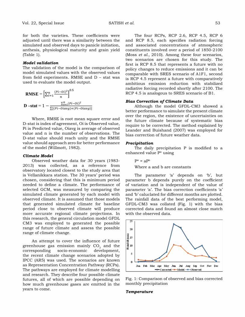
for both the varieties. These coefficients were adjusted until there was a similarity between the simulated and observed days to panicle initiation, anthesis, physiological maturity and grain yield (Table 1).

Model validation The validation of the model is the comparison of model simulated values with the observed values from field experiments. RMSE and D – stat was used to evaluate the model output.

Where, RMSE is root mean square error and D-stat is index of agreement, Oi is Observed value, Pi is Predicted value, Oiavg is average of observed value and n is the number of observations. The D-stat value should reach unity and the RMSE value should approach zero for better performance of the model (Willmott, 1982).

Climate ModelObserved weather data for 30 years (1983-

2013) was collected, as a reference from observatory located closest to the study area that is Vellanikkara station. The 30 years’ period was chosen, considering that this is minimum period needed to define a climate. The performance of selected GCM, was measured by comparing the simulated climate generated by each model with observed climate. It is assumed that those models that generated simulated climate for baseline period close to observed climate will produce more accurate regional climate projections. In this research, the general circulation model GFDL CM3 was employed to generated the possible range of future climate and assess the possible range of climate change.

An attempt to cover the influence of future greenhouse gas emission mainly CO2 and the corresponding socio-economic development, the recent climate change scenarios adopted by IPCC (AR5) was used. The scenarios are known as Representation Concentration Pathway (RCPs). The pathways are employed for climate modelling and research. They describe four possible climate futures, all of which are possible depending on how much greenhouse gases are emitted in the years to come.

The four RCPs, RCP 2.6, RCP 4.5, RCP 6 and RCP 8.5, each specifies radiation forcing and associated concentrations of atmospheric constituents involved over a period of 1850-2100 (Moss et al., 2010). Among these four scenarios, two scenarios are chosen for this study. The first is RCP 8.5 that represents a future with no policy changes to reduce emissions and it can be comparable with SRES scenario of A1F1, second is RCP 4.5 represent a future with comparatively ambitious emission reduction with stabilized radiative forcing recorded shortly after 2100. The RCP 4.5 is analogous to SRES scenario of B1.

Bias Correction of Climate DataAlthough the model GFDL-CM3 showed a

better performance to simulate the present climate over the region, the existence of uncertainties on the future climate because of systematic bias require to be corrected. The method explained by Leander and Buishand (2007) was employed for bias correction of future weather data.

Precipitation The daily precipitation P is modified to a

enhanced value P* using

P* = aPb

Where a and b are constants

The parameter ‘a’ depends on ‘b’, but parameter b depends purely on the coefficient of variation and is independent of the value of parameter ‘a’. The bias correction coefficients ‘a’ and ‘b’ caluclated for different months are plotted. The rainfall data of the best performing model, GFDL-CM3 was collated (Fig. 1) with the bias corrected data and found an almost close match with the observed data.

Fig. 1: Comparison of observed and bias corrected monthly precipitation

Temperature

Vol. 22, Special Issue SATISH et al. 53

54 June 2020

Correction for temperature requires shifting and scaling to modify the mean and the variance. The corrected daily temperature T* is given by:

Where Tmod is the daily temperature from GFDL-CM3 model and T0bs is the observed daily temperature.

Leander and Buishand (2007) found that a comparatively simple non-linear correction, adjusting both the biases within the mean and its variability, results in finer generation of observed extreme daily and multi-daily precipitation amounts than the regularly used linear scaling correction. This power law transformation method which corrects for the coefficient of variation (CV) and the mean of the precipitation data was utilized in this current study to correct bias in precipitation data. The most important statistics (coefficient of variation, mean and standard deviation of the model data) were closely matched with corresponding quantities calculated from the observed values was showed in Fig. 2 (a) & 2 (b).

Fig. 2 (a). Comparison of observed and bias corrected monthly maximum temperature

Fig. 2 (b). Comparison of observed and bias corrected monthly minimum temperature

reSuLtS aNd dISCuSSIoNChanges of climatic variables during the rice

growing period under RCP 4.5 and RCP 8.5

TemperatureDuring the D1 planting, maximum

temperatures of rice growing period under RCP 4.5 and 8.5 shown a difference of -0.1 0C (2050s), 0.3 0C (2080s) and 0.9 0C (2050s) and 1.8 0C (2080s) respectively, when differentiated with the year 2016. Whereas minimum temperature under RCP 4.5 and 8.5 shown a difference of 3.5 0C (2050s), 3.8 0C (2080s) and 4.2 0C (2050s), 5, 20C (2080s) compared to 22.3 0C in 2016. The similar trend of increasing maximum and minimum temperatures was observed in crop growing period of D2, D3, D4 and D5 planting under RCP 4.5 and 8.5 are showed in the Table 1.

Rainfall and Solar radiationUnder RCP 4.5 and 8.5 scenarios, rainfall

shown an increasing trend in each of the date of plantings. Whereas solar radiation shown a declining trend in all the dates of planting (Table 1). In D1 and D2 plantings, amount of solar radiation difference was higher in RCP 4.5 and 8.5 when refer to the year 2016. But, with the plantings D3, D4 and D5 the amount of solar radiation difference was less.

Crop model efficiency confirmationThe main driving factor of the study is not

to test the model (CERES-Rice) capability as the model has been (calibrated/validated/used for yield simulations) worked out for many places in India successfully where researchers established its usability for rice yield simulations (Satapathy et al. 2014; Singh et al., 2007 & 2016; Sudharshan et. al., 2013). However, the model was calibrated to derive the genetic coefficients using Gencalc (Hunt et al., 1993) for both varieties Jyothi and Kanchana (Table 2) under the department of Agricultural Meteorology, Thrissur, using the five years (2012-2016) crop data. In the present study, calibrated genetic coefficients of varieties Jyothi and Kanchana were employed to simulate the phenological stages and yields for future scenarios.

Impact of climate change on phenologyDays to panicle initiation, anthesis and

physiological maturity varies with planting dates for both varieties in projected RCP 4.5 and 8.5 scenarios.

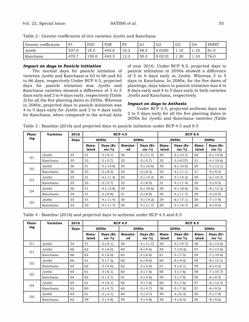
Impact on days to Panicle initiationThe normal days for panicle initiation of

varieties Jyothi and Kanchana is 63 to 66 and 62 to 66 days, respectively.Under RCP 4.5, projected days for panicle initiation was Jyothi and Kanchana varieties showed a difference of 3 to 5 days early and 2 to 4 days early, respectively (Table 3) for all the five planting dates in 2050s. Whereas in 2080s, projected days to panicle initiation was 4 to 5 days early for Jyothi and 2 to 4 days early for Kanchana, when compared to the actual data

of year 2016. Under RCP 8.5, projected days to panicle inititation in 2050s showed a difference of 5 to 6 days early in Jyothi. Whereas 3 to 5 days in Kanchana. In 2080s, for the five dates of plantings, days taken to panicle initiation was 6 to 8 days early and 4 to 5 days early in both varieties Jyothi and Kanchana, respectively.

Impact on days to AnthesisUnder RCP 4.5, projected anthesis days was

2 to 5 days early for all the five planting dates in 2050s for Jyothi and Kanchana varieties (Table

Table 2 : Genetic coefficients of rice varieties Jyothi and Kanchana

Genetic coefficients P1 P2O P2R P5 G1 G2 G3 G4 PHINTJyothi 537.0 18.5 445.0 10.2 48.5 0.0250 1.10 1.10 81.0Kanchana 470.7 150.0 445.5 12.3 50.5 0.0210 1.30 1.10 76.0

Table 3 : Baseline (2016) and projected days to panicle initiation under RCP 4.5 and 8.5

Plant-ing

varieties 2016 rCP 4.5 rCP 8.5

days 2050s 2080s 2050s 2080s

Simu-lated

days (er-ror %)

Simulat-ed

days (er-ror %)

Simu-lated

days (er-ror %)

Simu-lated

days (er-ror %)

D1Jyothi 34 31 -3 (-8.1) 30 -4 (-11.7) 29 -5 (-14.7) 28 -6 (-13.6)

Kanchana 35 33 -2 (-5.7) 33 -2 (-5.7) 32 -3 (-8.57) 31 -4 (-10.6)

D2Jyothi 36 31 -5 (-13.8) 30 -5 (-16.6) 30 -6 (-16.6) 29 -7 (-12.1)

Kanchana 36 33 -3 (-8.3) 33 -3 (-8.3) 32 -4 (-11.1) 31 -5 (-9.2)

D3Jyothi 35 31 -4 (-11.4) 30 -5 (-14.2) 30 -5 (-14.2) 29 -6 (-10.7)

Kanchana 35 33 -2 (-5.7) 32 -3 (-8.5) 31 -4 (-11.4) 30 -5 (-9.3)

D4Jyothi 36 31 -5 (-13.8) 30 -6 (-16.6) 30 -6 (-16.6) 28 -8 (-12.3)

Kanchana 34 31 -3 (-8.8) 31 -3 (-8.8) 30 -4 (-11.7) 29 -5 (-9.5)

D5Jyothi 35 31 -4 (-11.4) 30 -5 (-14.2) 29 -6 (-17.1) 28 -7 (-7.9)

Kanchana 34 30 -4 (-11.7) 30 -4 (-11.7) 29 -5 (-14.7) 28 -8 (-9.6)

Table 4 : Baseline (2016) and projected days to anthesis under RCP 4.5 and 8.5

Plant-ing


days 2050s 2080s 2050s 2080s

Simu-lated

days (er-ror %)

Simulat-ed

days (er-ror %)

Simu-lated

days (er-ror %)

Simu-lated

days (er-ror %)

D1 Jyothi 34 31 -3 (-8.1) 30 -4 (-11.7) 29 -5 (-14.7) 28 -6 (-13.6)

D1Jyothi 66 62 -4 (-6.0) 60 -6 (-9.0) 59 -7 (10.6) 57 -9 (-13.6)

Kanchana 66 62 -4 (-6.0) 62 -4 (-6.0) 61 -5 (-7.5) 59 -7 (-10.6)

D2Jyothi 66 61 -5 (-7.5) 60 -6 (-9.0) 60 -6 (-9.0) 58 -8 (-12.1)

Kanchana 65 62 -3 (-4.6) 62 -3 (-4.6) 61 -4 (-6.1) 59 -6 (-9.2)

D3Jyothi 65 61 -5 (-6.1) 60 -5 (-7.6) 60 -5 (-7.6) 58 -7 (-10.7)

Kanchana 64 62 -2 (-3.1) 61 -3 (-4.6) 59 -5 (-7.8) 58 -6 (-9.3)

D4Jyothi 65 61 -4 (-6.1) 60 -4 (-7.6) 60 -5 (-7.6) 57 -8 (-12.3)

Kanchana 63 60 -3 (-4.7) 60 -3 (-4.7) 58 -5 (-7.9) 57 -6 (-9.5)

D5Jyothi 63 61 -2 (-3.1) 60 -3 (-4.7) 59 -4 (-6.3) 58 -5 (-7.9)

Kanchana 62 59 -3 (-4.8) 59 -3 (-4.8) 58 -4 (-6.4) 56 -8 (-9.6)


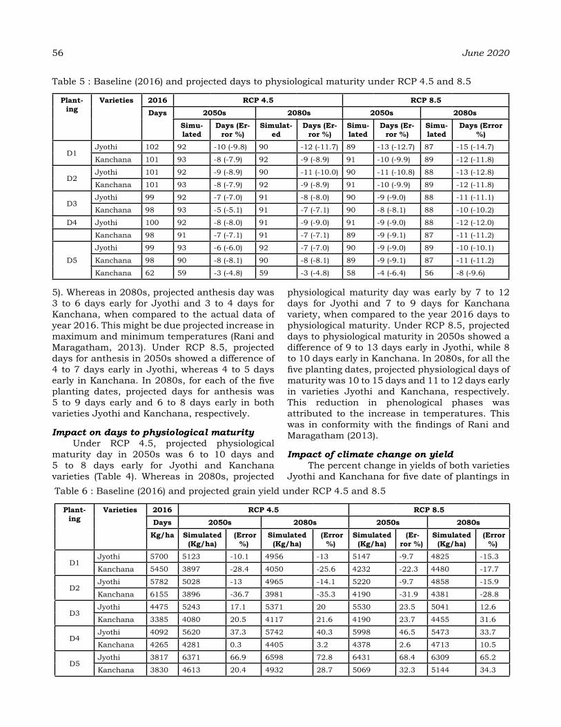
56 June 2020

5). Whereas in 2080s, projected anthesis day was 3 to 6 days early for Jyothi and 3 to 4 days for Kanchana, when compared to the actual data of year 2016. This might be due projected increase in maximum and minimum temperatures (Rani and Maragatham, 2013). Under RCP 8.5, projected days for anthesis in 2050s showed a difference of 4 to 7 days early in Jyothi, whereas 4 to 5 days early in Kanchana. In 2080s, for each of the five planting dates, projected days for anthesis was 5 to 9 days early and 6 to 8 days early in both varieties Jyothi and Kanchana, respectively.

Impact on days to physiological maturityUnder RCP 4.5, projected physiological

maturity day in 2050s was 6 to 10 days and 5 to 8 days early for Jyothi and Kanchana varieties (Table 4). Whereas in 2080s, projected

physiological maturity day was early by 7 to 12 days for Jyothi and 7 to 9 days for Kanchana variety, when compared to the year 2016 days to physiological maturity. Under RCP 8.5, projected days to physiological maturity in 2050s showed a difference of 9 to 13 days early in Jyothi, while 8 to 10 days early in Kanchana. In 2080s, for all the five planting dates, projected physiological days of maturity was 10 to 15 days and 11 to 12 days early in varieties Jyothi and Kanchana, respectively. This reduction in phenological phases was attributed to the increase in temperatures. This was in conformity with the findings of Rani and Maragatham (2013).

Impact of climate change on yield The percent change in yields of both varieties

Jyothi and Kanchana for five date of plantings in

Table 5 : Baseline (2016) and projected days to physiological maturity under RCP 4.5 and 8.5

Plant-ing


days 2050s 2080s 2050s 2080s

Simu-lated

days (er-ror %)

Simulat-ed

days (er-ror %)

Simu-lated

days (er-ror %)

Simu-lated

days (error %)

D1Jyothi 102 92 -10 (-9.8) 90 -12 (-11.7) 89 -13 (-12.7) 87 -15 (-14.7)

Kanchana 101 93 -8 (-7.9) 92 -9 (-8.9) 91 -10 (-9.9) 89 -12 (-11.8)

D2Jyothi 101 92 -9 (-8.9) 90 -11 (-10.0) 90 -11 (-10.8) 88 -13 (-12.8)

Kanchana 101 93 -8 (-7.9) 92 -9 (-8.9) 91 -10 (-9.9) 89 -12 (-11.8)

D3Jyothi 99 92 -7 (-7.0) 91 -8 (-8.0) 90 -9 (-9.0) 88 -11 (-11.1)

Kanchana 98 93 -5 (-5.1) 91 -7 (-7.1) 90 -8 (-8.1) 88 -10 (-10.2)

D4 Jyothi 100 92 -8 (-8.0) 91 -9 (-9.0) 91 -9 (-9.0) 88 -12 (-12.0)

Kanchana 98 91 -7 (-7.1) 91 -7 (-7.1) 89 -9 (-9.1) 87 -11 (-11.2)

D5

Jyothi 99 93 -6 (-6.0) 92 -7 (-7.0) 90 -9 (-9.0) 89 -10 (-10.1)

Kanchana 98 90 -8 (-8.1) 90 -8 (-8.1) 89 -9 (-9.1) 87 -11 (-11.2)

Kanchana 62 59 -3 (-4.8) 59 -3 (-4.8) 58 -4 (-6.4) 56 -8 (-9.6)

Table 6 : Baseline (2016) and projected grain yield under RCP 4.5 and 8.5

Plant-ing


days 2050s 2080s 2050s 2080s

Kg/ha Simulated (Kg/ha)

(error %)

Simulated (Kg/ha)

(error %)

Simulated (Kg/ha)

(er-ror %)

Simulated (Kg/ha)

(error %)

D1Jyothi 5700 5123 -10.1 4956 -13 5147 -9.7 4825 -15.3

Kanchana 5450 3897 -28.4 4050 -25.6 4232 -22.3 4480 -17.7

D2Jyothi 5782 5028 -13 4965 -14.1 5220 -9.7 4858 -15.9

Kanchana 6155 3896 -36.7 3981 -35.3 4190 -31.9 4381 -28.8

D3Jyothi 4475 5243 17.1 5371 20 5530 23.5 5041 12.6

Kanchana 3385 4080 20.5 4117 21.6 4190 23.7 4455 31.6

D4Jyothi 4092 5620 37.3 5742 40.3 5998 46.5 5473 33.7

Kanchana 4265 4281 0.3 4405 3.2 4378 2.6 4713 10.5

D5Jyothi 3817 6371 66.9 6598 72.8 6431 68.4 6309 65.2

Kanchana 3830 4613 20.4 4932 28.7 5069 32.3 5144 34.3

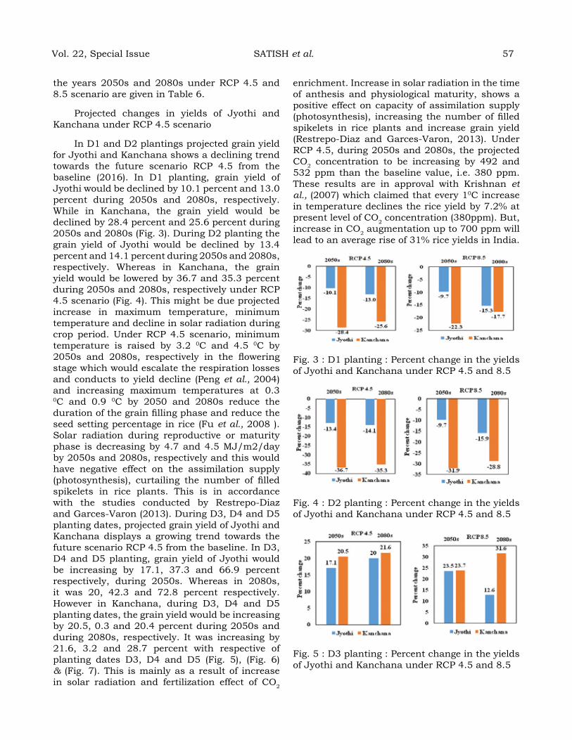
the years 2050s and 2080s under RCP 4.5 and 8.5 scenario are given in Table 6.

Projected changes in yields of Jyothi and Kanchana under RCP 4.5 scenario

In D1 and D2 plantings projected grain yield for Jyothi and Kanchana shows a declining trend towards the future scenario RCP 4.5 from the baseline (2016). In D1 planting, grain yield of Jyothi would be declined by 10.1 percent and 13.0 percent during 2050s and 2080s, respectively. While in Kanchana, the grain yield would be declined by 28.4 percent and 25.6 percent during 2050s and 2080s (Fig. 3). During D2 planting the grain yield of Jyothi would be declined by 13.4 percent and 14.1 percent during 2050s and 2080s, respectively. Whereas in Kanchana, the grain yield would be lowered by 36.7 and 35.3 percent during 2050s and 2080s, respectively under RCP 4.5 scenario (Fig. 4). This might be due projected increase in maximum temperature, minimum temperature and decline in solar radiation during crop period. Under RCP 4.5 scenario, minimum temperature is raised by 3.2 0C and 4.5 0C by 2050s and 2080s, respectively in the flowering stage which would escalate the respiration losses and conducts to yield decline (Peng et al., 2004) and increasing maximum temperatures at 0.3 0C and 0.9 0C by 2050 and 2080s reduce the duration of the grain filling phase and reduce the seed setting percentage in rice (Fu et al., 2008 ). Solar radiation during reproductive or maturity phase is decreasing by 4.7 and 4.5 MJ/m2/day by 2050s and 2080s, respectively and this would have negative effect on the assimilation supply (photosynthesis), curtailing the number of filled spikelets in rice plants. This is in accordance with the studies conducted by Restrepo-Diaz and Garces-Varon (2013). During D3, D4 and D5 planting dates, projected grain yield of Jyothi and Kanchana displays a growing trend towards the future scenario RCP 4.5 from the baseline. In D3, D4 and D5 planting, grain yield of Jyothi would be increasing by 17.1, 37.3 and 66.9 percent respectively, during 2050s. Whereas in 2080s, it was 20, 42.3 and 72.8 percent respectively. However in Kanchana, during D3, D4 and D5 planting dates, the grain yield would be increasing by 20.5, 0.3 and 20.4 percent during 2050s and during 2080s, respectively. It was increasing by 21.6, 3.2 and 28.7 percent with respective of planting dates D3, D4 and D5 (Fig. 5), (Fig. 6) & (Fig. 7). This is mainly as a result of increase in solar radiation and fertilization effect of CO2

enrichment. Increase in solar radiation in the time of anthesis and physiological maturity, shows a positive effect on capacity of assimilation supply (photosynthesis), increasing the number of filled spikelets in rice plants and increase grain yield (Restrepo-Diaz and Garces-Varon, 2013). Under RCP 4.5, during 2050s and 2080s, the projected CO2 concentration to be increasing by 492 and 532 ppm than the baseline value, i.e. 380 ppm. These results are in approval with Krishnan et al., (2007) which claimed that every 10C increase in temperature declines the rice yield by 7.2% at present level of CO2 concentration (380ppm). But, increase in CO2 augmentation up to 700 ppm will lead to an average rise of 31% rice yields in India.

Fig. 3 : D1 planting : Percent change in the yields of Jyothi and Kanchana under RCP 4.5 and 8.5




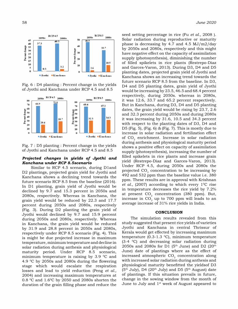
58 June 2020



Projected changes in yields of Jyothi and Kanchana under RCP 8.5scenario

Similar to RCP 4.5 scenario, during D1and D2 plantings, projected grain yield for Jyothi and Kanchana shows a declining trend towards the future scenario RCP 8.5 from the baseline (2016). In D1 planting, grain yield of Jyothi would be declined by 9.7 and 15.3 percent in 2050s and 2080s, respectively. Whereas in Kanchana, the grain yield would be reduced by 22.3 and 17.7 percent during 2050s and 2080s, respectively (Fig. 3). During D2 planting the grain yield of Jyothi would declined by 9.7 and 15.9 percent during 2050s and 2080s, respectively. Whereas in Kanchana, the grain yield would be reduced by 31.9 and 28.8 percent in 2050s and 2080s, respectively under RCP 8.5 scenario (Fig. 4). This is might be due projected increase in maximum temperature, minimum temperature and decline in solar radiation during anthesis and physiological maturity period. Under RCP 8.5 scenario, minimum temperature is raising by 3.9 0C and 4.9 0C by 2050s and 2080s during the flowering stage which would escalate the respiration losses and lead to yield reduction (Peng et al., 2004) and increasing maximum temperatures at 0.8 0C and 1.60C by 2050 and 2080s shorten the duration of the grain filling phase and reduce the

seed setting percentage in rice (Fu et al., 2008 ). Solar radiation during reproductive or maturity phase is decreasing by 4.7 and 4.5 MJ/m2/day by 2050s and 2080s, respectively and this might have negative effect on the capacity of assimilation supply (photosynthesis), diminishing the number of filled spikelets in rice plants (Restrepo-Diaz and Garces-Varon, 2013). During D3, D4 and D5 planting dates, projected grain yield of Jyothi and Kanchana shows an increasing trend towards the future scenario RCP 8.5 from the baseline. In D3, D4 and D5 planting dates, grain yield of Jyothi would be increasing by 23.5, 46.5 and 68.4 percent respectively, during 2050s. whereas in 2080s, it was 12.6, 33.7 and 65.2 percent respectively. But in Kanchana, during D3, D4 and D5 planting dates, the grain yield would be rising by 23.7, 2.6 and 32.3 percent during 2050s and during 2080s it was increasing by 31.6, 10.5 and 34.3 percent with respect to the planting dates of D3, D4 and D5 (Fig. 5), (Fig. 6) & (Fig. 7). This is mostly due to increase in solar radiation and fertilization effect of CO2 enrichment. Increase in solar radiation during anthesis and physiological maturity period shows a positive effect on capacity of assimilation supply (photosynthesis), increasing the number of filled spikelets in rice plants and increase grain yield (Restrepo-Diaz and Garces-Varon, 2013). Under RCP 4.5, during 2050s and 2080s the projected CO2 concentration to be increasing by 492 and 532 ppm than the baseline value i.e. 380 ppm. These results are in approval with Krishnan et al., (2007) according to which every 10C rise in temperature decreases the rice yield by 7.2% at present CO2 concentration (380 ppm). But, increase in CO2 up to 700 ppm will leads to an average increase of 31% rice yields in India.

CoNCLuSIoNThe simulation results revealed from this

study suggested that present rice yields of varieties Jyothi and Kanchana in central Thrissur of Kerala would get effected by increasing maximum temperature (0.3-1.3 0C), minimum temperature (3-4 0C) and decreasing solar radiation during 2050s and 2080s for D1 (5th June) and D2 (20th June) date of plantings where as the effect of increased atmospheric CO2 concentration along with increased solar radiation during anthesis and physiological maturity benefitted the yieldsof D3 (5th July), D4 (20th July) and D5 (5th August) date of plantings. If this situation prevails in future, change in the sowing window from the month of June to July and 1st week of August appeared to

be the best adaption to reduce the negative impact in future scenarios.

reFereNCeSFAOSTAT (2015). http://faostat3.fao.org/

browse/Q/QC/E.Fu, G. F., Tao, L. X., Song, J., Wang, X., Cao, L. Y.,

and Cheng, S. H. 2008: Responses of yield characteristics to high temperature during flowering stage in hybrid rice Guodao. Rice Sci. 15: 215-222.

Hunt, L. A., Pararajasingham, S., Jones, J. W., Hoogenboom, G., Imamura, D., T. & Ogoshi, R. M. (1993). GENCALC software to facilitate the use of crop models for analysing field experiments. Agronomy. J., 85: 1090–1094.

IPCC (2013). IPCC Fifth Assessment Report, Climatic Change 2013: The Physical Science Basis. Intergov. Panel Clim.Chang. AR5, pp. 31–39.

Krishnan, P., Swain, D. K., Bhaskar, B. C., Nayak, S. K., and Dash, R. N. (2007). Impact of elevated CO2 and temperature on rice yield and methods of adaptation as evaluated by crop simulation studies.Agric. Ecosyst. Environ, 122: 233-242.

Leander, R. and Buishand, T. A. (2007).Resampling of regional climate model output for the simulation of extreme river flows.J Hydrol, 332:487-496.

Lobell, D.B., Schlenker, W., Costa-Roberts, J., (2011). Climate trends and global crop production since 1980.Science, 333: 616–620.

Moss, H. R., Edmonds, J. A., Hibbard, A. K., Manning, R. M., Rose, K. S., Vuuren, P. D., Carter, R. T., Emori, S., Kainuma, M., Kram, T., Meehl, A. G., Mitchell, F. B. J., Nakicenovic, N., Raihi, K., Smith, J. S., Stouffer, J. R., Thomson, M. A., Weyant, P. J., and Wilbanks, J. T. (2010). The next generation of scenarios for climate change research and assessment. Nature, 463: 747-756.

Parry, M. L., Canziani, O. F., Palutikof, J. P., Van der Linden, P. J., and Hanson, C. E. (Eds.), 2007. Climate Change 2007.Impacts, Adaptation and Vulnerability.Cambridge University Press, 976 pp.

Peng, S, J., Huang, J. E., Sheehy, R. C., Laza, R. M., Visperas, X., Zhong, G. S., Centeno, G. S., Khush, K. G., and Cassman (2004). Rice yields decline with higher night temperature from global warming. Proceedings of the NationalAcademy of Sciences of the United States of America, 101: 9971-9975.

Rani, B. A. and Maragatham, N. 2013.Effect of elevated temperature on rice phenology and yield.Indian J. Sci. and Technol. 6 (8): 5095-5097.

Restrepo-Díaz, H. and Garces-Varon, H. (2013). Response of rice plants to heat stress during initiation of panicle primordia or grain-filling phases. J Stress Physiol. Biochem, 9: 318-325.

Satapathy, S S., Swain, D. K., and Herath, S. (2014). Field experiments and simulation to evaluate rice cultivar adaptation to elevated carbon dioxide and temperature in sub-tropical India.Eur J Agron, 54: 21– 33.

Singh, H., Singh, K. N., and Hasan, B. (2007).Evaluation of CERES-Rice model (V. 4.0) under temperate conditions of Kashmir valley, India. Cereal Research Communications, 35 (4) :1723-1732.

Singh, P. K., Singh, K. K., Rathore, L. S., Baxla, A. K., Bhan, S. C., Akhilesh, G., Gohain, G. B., Balasubramanian, R., Singh, R. S., and Mall., R. K. (2016). Rice (OryzasativaL.) yield gap using the CERES-rice model of climate variability for different agroclimatic zones of India. CurrentScience, 110 (3) : 405-413.

Srivastava, A., Naresh Kumar, S., Aggarwal, P.K. (2010). Assessment on vulnerability of sorghum to climate change in India.Agric. Ecosyst. Environ, 138: 160–169.

Soora, N.K., Aggarwal, P.K., Saxena, R., Rani, S., Jain, S., Chauhan, N. (2013). An assessment of regional vulnerability of rice to climate change in India.Clim. Chang, 118: 683–699.

Sudharsan, D., Adinarayana, J., Reddy, D.R., Sreenivas, G., Ninomiya, S., Hirafuji, M., Kiura, T., Tanaka, K., Desai, U.B., Merchant, S.N. (2013). Evaluation of weather-based rice yield models in India. Int. J. Biometeorol, 57: 107–123.

Willmott, C. J. (1982). Some comments on the evaluation of model performance. Am. Meteorol. Soc. Bull, 63: 1309-1313.


Impact of Climate variability on Species abundance of rice Insect Pests across agro Climatic Zones of India

veNNILa S, ShaBIStaNa NISar, MurarI KuMar, Yadav SK, PauL rK1, SrINIvaSa rao M2 aNd PraBhaKar M2

ICAR- National Research Centre for Integrated Pest Management, New Delhi 1ICAR- Indian Agricultural Statistics Research Institute, New Delhi

2ICAR- Central Research Institute for Dryland Agriculture, HyderabadE-mail: [email protected]

aBStraCtImpact of changing temperature and rainfall on abundance of four rice insect pests viz., yellow stem borer (YSB), leaf folder (LF), brown plant hopper (BPH) and green leafhopper during kharif 2011-16 was assessed for seven rice growing locations in India. While YSB and GLH had maximum abundance at Chinsurah (West Bengal) and Raipur (Chatisgarh), respectively Ludhiana (Punjab) had the highest LF and BPH abundance. Magnitude of variability of maximum temperature (MaxT0C), minimum temperature (MinT0C) and rainfall (RF mm) quantified for 2011-16 over long term ‘normals’ showed significant spatial heterogeneity with all three variables significantly increasing at Karjat (Maharashtra) and Kampasagar (Telangana). None of the variables had significance at Chinsurah (WB). Three, five and two locations had increasing MaxT (1.4-3.60C), MinT (-0.58-1.850C) and RF (42.8–84.8mm/week), respectively. Kendall’s τ correlations between abundance of each insect and deviations of climatic values derived for MaxT, MinT and RF on weekly basis had also shown spatially variable significance with 78% associations negative indicating decreasing species abundance in relation to changing climate. Increasing YSB and GLH with increasing MaxT (0.270C) and MinT (0.930C) at Raipur (CG) and of LF at Aduthurai (Tamilnadu) with increasing rainfall (5.43 mm/week) revealed their increasing importance from pest management perspective.

Keywords: Climate variability, Species abundance, Rice, Yellow stem borer, Leaf folder, Brown plant hopper, Green leafhopper

INtroduCtIoN

Climate determines the geo-diversity and evolutionary adaptability of insects in the regions of high climatic variations such as hot semi-arid and hot humid eco-regions prone to low and uncertain rainfall, implying water shortage contrast to high flooding in tropical and temperate regions. Intensity and frequency pattern of precipitation, drought and solar radiations affect the appearance, abundance, severity and outbreak of insect pests and associated friendly arthropods. Manmade interventions such as crop diversity, cropping intensity, varietal selection, irrigation, fertilization and use of other management practices influence ecological dependence of species in positive or negative terms (Carol Shennan, 2008). Climate change directly influences the insect physiology and behaviour (Samways, 2005; Parmesan, 2007; Merrill et al., 2008), or may be indirectly through host plants and natural enemies (Harrington et al., 2001;Bale et al., 2002; Bale and Hayward, 2010). Host plants, natural enemies and extreme weather conditions manipulate species abundance of insects (Kambrekar et al., 2015) and leads to rapid

changes in dynamics of species. Because of these tight ecological significances, interplay between plants and weather conditions plays a crucial role in insect attaining pest status as they become more susceptible to perturbations of climate change (Woiwod, 1997; Coley, 1998). Daniela Salite (2019) reported that weather and climatic variability are co-operative environmental situations accounting to pest vulnerability. Moreover, local adaptation determines the potential of insect populations to respond to environmental changes, their vulnerability and bio-geographical shifts under climate change scenario (Razgour et al., 2019).

Rice is grown in varied climatic zones and ecoregions in India with an area, production and productivity of 43.4 million hectares, 104.3 million tonnes and 2404 kg/ha, respectively (Anonymous, 2017). More than 100 species of insects attack rice crop with twenty of them causing economic damage. Insect pests that cause significant yield losses in rice crop are stem borers, leafhoppers, plant hoppers, gall midge, defoliators, and grain-sucking bugs (Pathak and Khan, 1994). Lepidopterans viz., Scirpophaga incertulus


(Walker) (yellow stemborer), Cnaphalocrocis medinalis (Guenee) (leaf folder) and homopterans particularly Nilaparvata lugens (Stal), (brown planthopper) and Nephotettix virescens Distant (green leafhopper) cause 15-60% of economic yield losses in rice (Krishnaiah and Varma, 2012). In rice ecosystem, the population abundance of insects are monitored on daily basis using light traps and it is the weekly total expressed as numbers/trap/week, that are often used for comparisons (Vennila et al., 2016). Impact of climate change on population abundance of rice insects can have an effect on individual organism or interaction of species invading the rice ecosystem (Huang et al., 2010). Present study investigated the impact of climatic variability on population abundance of four important insect pests from among different agro climatic zones growing rice in India.

MaterIaLS aNd MethodSSeven different rice growing locations

belonging to different agro climatic zones (ACZ) of India viz., (1) Ludhiana (Punjab) [30°54’N, 75°48’E; ACZ:Trans-Gangetic plain region], (2) Chinsurah (West Bengal) [22°.90’ N, 88°.38’ E; ACZ: Lower Gangetic plain region], (3) Raipur [21°.25’ N, 81°.62’ E; ACZ: Eastern plateau and hill region], (4) Karjat (Maharashtra) [18°.91’ N, 73°.33’ E;ACZ: West Coast Plains and Ghat Region], (5) Kampasagar (Telangana) [17°.37’ N, 78°.48’ E ; ACZ: Southern Plateau and Hills Region], (6) Mandya (Karnataka) [12°.52’ N, 76°.90’ E; ACZ: Southern Plateau and Hills Region]and (7) Aduthurai (Tamil Nadu) [11°.01’ N, 79°.30’ E; ACZ: East coast plain and hill region) constituted study locations. Abundance of adults of rice insect pests belonging to Lepidoptera [yellow stem borer: Scirpophaga incertulus (Walker) and leaf folder: Cnaphalocrocis medinalis (Guenee) ] and Homoptera [brown plant hopper: Nilaparvata lugens (Stal) and green leafhopper Nephotettix virescens Distant] recorded on daily basis from rice crop at the study locations using light traps (Chinsurah type) in kharif season of 2011-16 constituted the insect database. Although light trap catches are recorded daily, the population of insects caught in light traps, per trap, per week are used to express species abundance in a rice ecosystem.

Data on weather parameters viz., maximum temperature (MaxT 0C), minimum temperature (MinT 0C) and rainfall (RF mm) across study locations for kharif season of 22-44 standard

meteorological weeks (SMW) were collected simultaneously with insect data. Climatic variability with respect of MaxT, MinT and RF for study locations was worked out as deviations of actual weather values of kharif season of 2011-2016 from long term (40 years:1970-2010) normals for the same period and analysed using student ‘t’ test to determine the magnitude of change and its significance. Kendall’s tau (τ) correlations were worked out between deviations of climatic values derived for variables of MaxT, MinT and RF and abundance of each insect species on SMW basis for kharif season of 2011-16 for each study location to assess the impact of climatic variability on abundance of four study insects.

reSuLtS aNd dISCuSSIoNEffects of temperature on insects, like

changes in geographical range, overwintering, population growth rates, number of generations, crop-pest synchrony, dispersal and migration, availability of host plants and refugia are well known (Porter et al., 1991). Climate change is expected to impact the abundance, distribution range and phenology of many lepidopteran and homopteran insects (Andrew and Hughes 2005; Kocsis and Hufnagel, 2011; Baker et al., 2015). Abundance of adults of yellow stem borer (YSB), leaf folder (LF), brown plant hopper (BPH) and green leafhopper (GLH) during recent seasons (2011-16) in rice ecosystem of different study locations indicated that the relative importance of insects varied between locations of different ACZs as well as within ACZ (Table 1 & Fig. 1).Overall, the abundance of insect species in rice ecosystem followed the order YSB>LF for lepidopterans and BPH>GLH for homopterous insects. While YSB was abundant at Chinsurah (WB) (155.7 adults/trap/week), least was noticed at Ludhiana (PB) (2.07 adults/trap/week) with its insignificant presence at Mandya (KA). The order of importance for YSB was Chinsurah (WB) > Raipur (CG) >Aduthurai (TN) >Kampasagar (TS) > Ludhiana (PB). On the other hand, LF was the highest in abundance at Ludhiana (PB) (70. 6 adults/trap/week) followed by Chinsurah (WB) (18.0 adults/trap/week) with rest of the locations having a lower abundance (<10 adults/trap/week). Mandya (KA) was also free from the LF. Among homopterans, population of BPH was abundant at Ludhiana (PB), (1284 adults/trap/week) followed by Chinsurah (WB) (141.7 adults/trap/week), Kampasagar (TS) (135.6 adults/trap/week) and Aduthurai (TN) (61 adults/trap/week). Raipur (CG), Karjat (MH)

Vol. 22, Special Issue VENNILA et al. 61

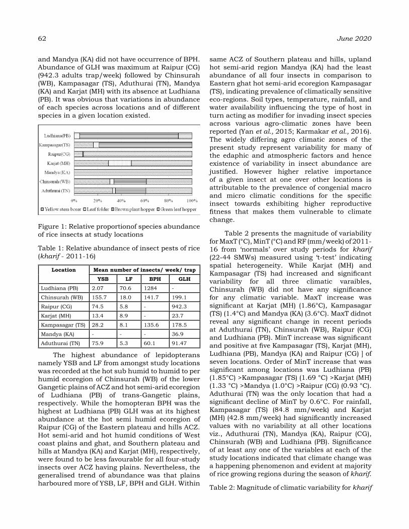
62 June 2020

and Mandya (KA) did not have occurrence of BPH. Abundance of GLH was maximum at Raipur (CG) (942.3 adults trap/week) followed by Chinsurah (WB), Kampasagar (TS), Aduthurai (TN), Mandya (KA) and Karjat (MH) with its absence at Ludhiana (PB). It was obvious that variations in abundance of each species across locations and of different species in a given location existed.

Figure 1: Relative proportionof species abundance of rice insects at study locations

Table 1: Relative abundance of insect pests of rice (kharif - 2011-16)

Location Mean number of insects/ week/ trap

YSB LF BPh gLh

Ludhiana (PB) 2.07 70.6 1284 -

Chinsurah (WB) 155.7 18.0 141.7 199.1

Raipur (CG) 74.5 5.8 - 942.3

Karjat (MH) 13.4 8.9 - 23.7

Kampasagar (TS) 28.2 8.1 135.6 178.5

Mandya (KA) - - - 36.9

Aduthurai (TN) 75.9 5.3 60.1 91.47

The highest abundance of lepidopterans namely YSB and LF from amongst study locations was recorded at the hot sub humid to humid to per humid ecoregion of Chinsurah (WB) of the lower Gangetic plains of ACZ and hot semi-arid ecoregion of Ludhiana (PB) of trans-Gangetic plains, respectively. While the homopteran BPH was the highest at Ludhiana (PB) GLH was at its highest abundance at the hot semi humid ecoregion of Raipur (CG) of the Eastern plateau and hills ACZ. Hot semi-arid and hot humid conditions of West coast plains and ghat, and Southern plateau and hills at Mandya (KA) and Karjat (MH), respectively, were found to be less favourable for all four-study insects over ACZ having plains. Nevertheless, the generalised trend of abundance was that plains harboured more of YSB, LF, BPH and GLH. Within

same ACZ of Southern plateau and hills, upland hot semi-arid region Mandya (KA) had the least abundance of all four insects in comparison to Eastern ghat hot semi-arid ecoregion Kampasagar (TS), indicating prevalence of climatically sensitive eco-regions. Soil types, temperature, rainfall, and water availability influencing the type of host in turn acting as modifier for invading insect species across various agro-climatic zones have been reported (Yan et al., 2015; Karmakar et al., 2016). The widely differing agro climatic zones of the present study represent variability for many of the edaphic and atmospheric factors and hence existence of variability in insect abundance are justified. However higher relative importance of a given insect at one over other locations is attributable to the prevalence of congenial macro and micro climatic conditions for the specific insect towards exhibiting higher reproductive fitness that makes them vulnerable to climate change.

Table 2 presents the magnitude of variability for MaxT (°C), MinT (°C) and RF (mm/week) of 2011-16 from ‘normals’ over study periods for kharif (22-44 SMWs) measured using ‘t-test’ indicating spatial heterogeneity. While Karjat (MH) and Kampasagar (TS) had increased and significant variability for all three climatic varaibles, Chinsurah (WB) did not have any significance for any climatic variable. MaxT increase was significant at Karjat (MH) (1.86°C), Kampasagar (TS) (1.4°C) and Mandya (KA) (3.6°C). MaxT didnot reveal any significant change in recent periods at Aduthurai (TN), Chinsurah (WB), Raipur (CG) and Ludhiana (PB). MinT increase was significant and positive at five Kampasagar (TS), Karjat (MH), Ludhiana (PB), Mandya (KA) and Raipur (CG) ] of seven locations. Order of MinT increase that was significant among locations was Ludhiana (PB) (1.85°C) >Kampasagar (TS) (1.69 °C) >Karjat (MH) (1.33 °C) >Mandya (1.0°C) >Raipur (CG) (0.93 °C). Aduthurai (TN) was the only location that had a significant decline of MinT by 0.6°C. For rainfall, Kampasagar (TS) (84.8 mm/week) and Karjat (MH) (42.8 mm/week) had significantly increased values with no variability at all other locations viz., Aduthurai (TN), Mandya (KA), Raipur (CG), Chinsurah (WB) and Ludhiana (PB). Significance of at least any one of the variables at each of the study locations indicated that climate change was a happening phenomenon and evident at majority of rice growing regions during the season of kharif.

Table 2: Magnitude of climatic variability for kharif

2011-16 across locations

Location actual weather Climatic deviationsMaxt (°C)

Mint (°C)

rF (mm/week)

Maxt (°C)

Mint (°C)

rF (mm/week)

Ludhi-ana (PB)

33.4 23 23.7 0.02 1.85** 7.38

Chinsur-ah (WB)

31.2 23.3 52.4 -0.4 -0.76 8.99

Raipur (CG)

30.8 22.2 49.3 0.27 0.93* 9.51

Karjat (MH)

31.6 23.7 153.6 1.86** 1.33** 42.8**

Kampas-agar (TS)

34.3 25.6 109.9 1.37** 1.69** 84.8**

Mandya (KA)

30.4 18.5 15.7 3.60** 1.09** -0.78

Aduthu-rai (TN)

34.3 24.8 25.7 -0.18 -0.58** 5.43

* & **: significance of climatic deviations from actual weath-er based on ‘t’ test at p<0.05 & 0.01

Kendall’s “Tau” estimates between each of MaxT, MinT and RF with abundance of both Lepidopterans (YSB and LF) (Table 3) showed significant and positive associations of YSB with increasing MaxT (0.27°C) and MinT (0.93°C) at Raipur (CG) implying increased abundance of YSB between 2011-16 in tune with increasing temperature. On the other hand, the non-significantly declining MinT (-0.76°C) at Chinsurah (WB) and significantly declining MinT (-0.58°C) at Aduthurai (TN) had decreasing effect on YSB. The association of leaf folder with climatic deviations was significantly positive only with MaxT (although magnitude of increase was not significant) at Raipur (CG). Leaf folder associations were significantly negative at Ludhiana (PB), Chinsurah (WB) and Aduthurai (TN) with MaxT although, magnitude of variability was non-significant at these locations. All significant associations of leaf folder with MinT were negative and were observed at Chinsurah (WB), Kampasagar (TS) and Aduthurai (TN) where the magnitude of MinT change was non significant, positive and negatively significant, respectively indicating the importance of MinT over MaxT in influencing leaf folder. Increasing RF (5.43 mm/week) had shown significantly positive association with LF at the Eastern coastal plain location of Aduthurai (TN) with hot sub humid to semi-arid ecoregion. Increased temperatures with increasing insect populations and pest outbreaks threaten food security (Jamieson et al., 2012) and lead to early and frequent application of insecticides under changing climate (Nansen and Smith, 2013). Increased temperatures accelerate the life cycles of plant species (Parmesan and Yohe, 2003; Willis

et al., 2008) significantly, influencing the feeding potential and reproduction pattern in insect pests. Irrespective of the specific causes, present study highlights the direct proportionality of temperature with species abundance of YSB and LF in general but, variable across locations. Increasing YSB and LF at Raipur (CG) and decreasing LF at Ludhiana (PB) and Chinsurah (WB) have significance from their management perspective. At Aduthurai (TN), it has to be remembered that the interplay of declining temperature and increasing rainfall would determine the abundance of leaf folder.

Table 3: Relation between insect abundance & climatic variability: Lepidopterans

In-sect

Location Mean nos/

week/ trap

Kendall’s ‘tau’ correla-tion coefficients

Maxt (°C)

Mint (°C)

rF (mm/week)

YSB

Ludhiana (PB) 2.07 -0.03 0.05 0.05Chinsurah (WB)

155.7 -0.08 -0.26* (-0.7)

-0.04

Raipur (CG) 74.2 0.22* (0.27)

0.14* (0.93*)

-0.11

Karjat (MH) 13.3 -0.07 0.08 0.10Kampasagar (TS)

28.2 0.01 0.03 -0.03

Aduthurai (TN)

59.1 -0.11 -0.25* (-0.58*)

0.09

LF

Ludhiana (PB) 53.9 -0.12* (0.02)

-0.08 0.05

Chinsurah (WB)

18 -0.17* (-0.40)

-0.31* (-0.76)

-0.05

Raipur (CG) 5.8 0.18* (0.27)

-0.07 -0.05

Karjat (MH) 8.9 0.05 -0.06 0.05Kampasagar (TS)

8.1 -0.05 -0.15* (1.69**)

-0.04

Aduthurai (TN)

5.5 -0.16* (-0.27)

-0.18* (-0.58**)

0.16* (5.43)

* & **: significance of ‘tau’ correlation coefficients at p<0.05 & 0.01; Figures in parentheses are the magnitude of climatic variability mentioned wherever the tau coefficients were significant and associated * & ** indicates the significance at p<0.05 & 0.01 based on ‘t’ test.

Amongst relations of climatic variables with abundance of Homopterans (Table 4), only Kampasagar (TS) had significant but negative associations of BPH with both MaxT (1.37°C) and MinT (1.69°C). On the contrary declining MinT (-0.8°C) at Chinsurah (WB) also had negative impact on BPH. Raipur (CG) alone had significant and positive associations of GLH with MaxT (0.3°C) and Min T (0.9°C).MaxT and MinT relations with GLH at Chinsurah (WB) were negatively significant. Increasing MaxT (3.6°C) at Mandya (KA) and


64 June 2020

declining MinT (- 0.58°C) at Aduthurai (TN) had significant and negative effects on GLH. In addition, increasing (84.8 mm/week) and decreasing (-0.78 mm/week) RF in Kampasagar (TS) and Mandya (KA) respectively, had significantly reduced GLH abundance. Except, for Raipur (CG), all other locations had declining GLH and it was expected that the diseases transmitted by them would also be generally on the decline although the effects of climatic variables of significance could be different on the premise of virus-vector relations. Changes in species abundance can aggravate the transmission of viruses (Timoney, 2003; Petzoldt and Seaman, 2010; Sharma, 2014). Climate change affects vectors also through modification of vector’s phenology, over-wintering, density, migration (Tanmoy et al., 2016). Phenology and physiology of the host when affected by climate change lead to differential virus susceptibility and virus ability to infect. Therefore, reducing abundance of GLH at Raipur (CG) should be observed with caution.

Table 4: Relation between insect abundance & climatic variability: Homopterans

In-sect

Location Mean nos/

week/ trap

Kendall’s ‘tau’ correlation coefficients

Maxt (°C)

Mint (°C)

rF (mm/week)

BPH

Ludhiana (PB)

1052 -0.11 -0.09 0.08

Chinsurah (WB)

141.7 -0.06 -0.27* (-0.8)

-0.04

Kampasagar (TS)

135.6 -0.13* (1.37**)

-0.26* (1.69**)

-0.02

Aduthurai (TN)

61.1 -0.01 -0.13 -0.05

GLH

Chinsurah (PB)

199.1 -0.13* (-0.4)

0.27* (-0.80)

-0.04

Raipur (CG) 880 0.16* (0.3)

0.12* (0.90)

-0.09

Karjat (MH) 23.7 0.07 0.04 0.01

Kampasagar (TS)

178.5 0.10 0.02 -0.16* (84.8**)

Mandya (KA)

5.2 -0.16* (3.6**)

-0.03 (1.09**)

-0.17* (-0.78)

Aduthurai (TN)

97.1 -0.12 -0.15* (-0.58**)

0.10

* & **: significance of ‘tau’ correlation coefficients at p<0.05 & 0.01; Figures in parentheses are the magnitude of climatic variability mentioned wherever the tau coefficients were significant and associated ** indicates the significance at p<0.05 based on ‘t’ test.

The impact of significantly increasing and declining climatic variables of recent periods on rice insect pests are summarised in Tables (5 & 6) for easy comprehension. The increasing temperature effects (both MaxT and/or MinT) at Raipur (CG) had led to increased abundance of YSB, LF and GLH and that of rainfall at Aduthurai (TN) had resulted in increased LF. Increasing magnitude of MaxT had decreasing effects on LF at Ludhiana (PB) and on BPH and GLH at Kampasagar (TS) and Mandya (KA). Increasing MinT had reducing effect on leaf folder and BPH at Kampasagar (TS). Nonetheless, increasing rainfall had decreasing effect on GLH at Kampasagar (TS) and Mandya (KA). Chinsurah (WB) and Aduthurai (TN) are the only two locations wherein the significantly declining climate variables viz., Max T and MinT had shown significant reducing effects. While both MaxT and MinT reductions at the two locations were significant for LF, the former had significance with GLH at Chinsurah (WB) and the later with YSB, GLH and BPH at both locations. Present study across seven different locations using four rice insect species had shown of climatic variability influence on species abundance to be largely negative (78%) implying lesser abundance of the study insects under changing climate. In other words, impact of climatic variability in 22% of cases over locations and insects had increasing effect over the recent periods of 2011-16.

Table 5: Significant impact of increasing climatic variability on rice insect pests

Climatic variable

Insects effect on insects

Location

MaxT (°C)

YSB, LF & GLH

Increase Raipur (CG)

LF, BPH & GLH

Decrease Ludhiana (PB), Kampasagar (TS) andMan-dya (KA)

MinT (°C)

YSB & GLH Increase Raipur (CG)

LF & BPH Decrease Kampasagar (TS)

RF (mm/week)

LF Increase Aduthurai (TN)

GLH Decrease Kampasagar (TS) andMan-dya (KA)

Table 6: Significant impact of decreasing climatic variability on rice insect pests

Climatic variable

Insects effect on insects

Location

MaxT (°C)

LF Decrease Chinsurah (WB) and Aduthurai (TN)

GLH Chinsurah (WB)

Min.T (°C) YSB, LF, BPH & GLH

Chinsurah (WB) andAduthurai (TN)

Altered climatic conditions influence the phenology of insects including early arrival and emergence time of insect pests (Dewar and Watt, 1992; Whittaker and Tribe, 1996). In the present study, evidences exist on the increasing abundance of YSB, LF and GLH at Raipur (CG) in relation to increased temperatures and of LF at Aduthurai (TN) with increasing rainfall at humid (semi/sub) ecoregions. The non-significant associations of insects with significantly changing climatic variables only imply the adaptability/resilience of the insects to the changing climate as on date. Strategizing future research and development efforts for integrated pest management (IPM) require assessment of effects of climate change at field level (Sharma and Prabhakar, 2014) and rice ecosystems deserve attention. Monitoring of species abundance of rice insects in climatically sensitive areas of hot semi-arid and hot humid ecoregions where climatic variability were documented provide indications of field level climate change impacts on changing rice insect pest scenario. The development of herbivore insect depends on the adaptation to both the environmental conditions and the host plant, physiological changes related to host-suitability and nutritional status (Hare, 1992; Roth and Lindroth, 1995; Coviella and Trumble, 1999; Gutierrez et al., 2008). Present study had unilaterally quantified the magnitude of change in climatic variables and direct effects on the four species of rice insect pests without accounting the host plant mediated factors such as phenology of rice crop in tune with the observed climatic variability. Nevertheless, species abundance at a given point of time is the manifestation of the cumulative factors (biotic and abiotic) impinging on the ecosystem reflected on ecological and evolutionary aspects of insect species. To predict the impact of climate variability on species abundance quantifying the climatic sensitivity of their activities like dispersion, reproduction and

foraging is essential. The relationship between climatic sensitivity and population performance in immatures and adults with respect to operative temperature in microenvironment of crop aid in prediction and evaluation of vulnerability to changing weather and climate (Kingsolver et al., 2011). The quantified impacts of climatic variables on rice insect pests of the present study across locations from different agro climatic zones portrayed the spatial heterogeneity not only associated with changing climate but also with their effects on rice insect pests notwithstanding, the fact that relative importance of insects species are different at different locations. With so much of the interacting forces determining species abundance in rice fields that are differ over space, components of pest management and frequency of interventions would also vary at different regions. Precise understanding and ranking of factors impinging species abundance of rice insects at each of locations/agro climatic zones are must in the context of climate change. There is need for integration of varied research findings available so far at each of the locations and insect species to synthesis a meaningful conclusion on pest management. Future plant protection is expected to evolve along the holistic approach of studying the effects, effectiveness and efficiency of all possible system variables whether natural or manmade determining the abundance of insect pests not to discount the within and between interactions among trophic levels of the rice ecosystem.

aCKNoWLedgeMeNtSAuthors gratefully acknowledge the funding

by Indian Council of Agricultural Research through National Innovations in Climate Resilient Agriculture Project with its implementation facilitated by Central Research Institute for Dryland Agriculture, Hyderabad. In addition, we gratefully appreciate the efforts of field staff and project centres of study locations for their contributions to database.

reFereNCeSAndrew, N.R and Hughes, L. (2005). Diversity

and assemblage structure of phytophagous Hemiptera along a latitudinal gradient: predicting the potential impacts of climate change. Global Ecol Biogeogr., 14: 249–262.

Anonymous (2017). Agricultural Statistics at a Glance 2017. Directorate of economics


66 June 2020

and statistics, Department of Agriculture and cooperation and farmer’s welfare, Government of India.

Bale, J. S and Hayward, S. A. L. (2010). Insect overwintering in a changing climate. The J. Exp. Biol., 213: 980-994.

Bale, J., Masters, G. J., Hodkins, I. D., Awmack, C., Bezemer, T. M., Brown, V. K., Buterfield, J., Buse, A., Coulson, J. C., Farrar, J., Good, J. E. G., Harrigton, R., Hartley, S., Jones, T. H., Lindroth, R. L., Press, M. C., Symrnioudis, I., Watt, A. D and Whittaker, J. B. (2002). Herbivory in global climate change research: Direct effects of rising temperature on insect herbivores. Global Change Biol., 8:1-16.

Carol Shennan (2008). Biotic interactions, ecological knowledge and agriculture. Phil. Trans. R. Soc., 363:717–739.

Coley, D. D. (1998). Possible effects of climate change on plant/herbivore interactions in moist tropical forests. Climatic change, 39 (2-3) :455-472.

Coviella, C.E and Trumble, J.T. (1999). Effects of elevated atmospheric CO2 on insect-plant interactions. Conservation Biol., 13 (8) : 1-13.

Daniela Salite (2019). Traditional prediction of drought under weather and climate uncertainty: analyzing the challenges and opportunities for small-scale farmers in Gaza province, southern region of Mozambique. Natural Hazards, 96 (3) :1289-1309.

Dewar, R.C and Watt, A.D. (1992). Predicted changes in the synchrony of larval emergence and budburst under climatic warming. Oecologia, 89, 557–559.

Gutierrez, A.P., Pointi, L., D’Oultremont, T and Ellis, C.K. (2008). Climate change effects on poikilothermtritrophic interactions. Climate change, 87: 67-92.

Hare, J.D. (1992). Effects of plant variation on herbivore-natural enemy interactions. In: Plant Resistance to Herbivores and Pathogens: Ecology, Evolution and Genetics. (Eds. Fritz, R.S., Simms, E.L.), University of Chicago Press, Chicago, Illinois, USA, pp. 278-298.

Harrington, R., Clark, S.J., Weltham, S.J., Virrier, P.J., Denhol, C.H., Hull, È. M., Maurice, D., Roun-sevell, M.D and Cocu, N. (2007). Environmental change and the phenology

of European aphids. Global Change Biol., 13:1556-1565.

Huang, Y., Stephan, L., Jonathan. P. G., John, D., and Anderson, J. (2010). Separation of longwave climate feedbacks from spectral observations, J. Geophys. Res., 115, https://doi.org/10.1029/2009JD012766.

Jamieson, M. A., Amy, M. Trowbridge, Kenneth, F. Raffa and Richard, Lindroth L. (2012). Consequences of climate warming and altered precipitation patterns for plant-Insect and multitrophic interactions. Plant Physiol., 160:1719–1727.

Kambrekar, D. N., Guledgudda, S. S., Anand, Kand Mohan, K. (2015). Impact of climate change on insect pests and their natural enemies. Kar. J. Agric. Sci., 28 (5) :814-816.

Karmakar, R., Indranil, D., Debashis, D and Amitava, R. (2016). Potential Effects of Climate Change on Soil Properties: A Review. Sci. Int., 4 (2) : 51-73.

Kingsolver, J. G., Arthur, H. W., Lauren, B., Buckley, Kristen, A., Potter, Heidi, J., MacLeanand Jessica K. H. (2011). Complex life cycles and the responses of insects to climate change. Integr Comp Biol., 51 (5) :719-732. doi: 10.1093/icb/icr015.

Kocsis, M andHufnagel, L. (2011). Impacts of climate change on lepidoptera species and communities. App. Eco. Env Res., 9 (1) : 43-72.

Krishnaiah, K and Varma, N. R. G. (2012). Changing insect pest scenario in the rice ecosystem –A national perspective. Directorate of Rice Research Rajendranagar, Hyderabad.pp.2-8.

Merrill, R., Gutieyrrez, D., Lewis, O., Gutieyrrez. J., Diez, S and Wilson, R. (2008). Combined effects of climate and biotic interactions on the elevational range of a phytophagous insect. J. Animal Ecol., 77:145-155.

Nansen, C and Smith. R.T. J. (2013). The performance of insecticides–a critical review: Insecticides (Ed. by S Trdan) InTech Europe.pp.195-232.

Parmesan, Cand Yohe, G. (2003). A globally coherent fingerprint of climate change impacts across natural systems. Nature, 421:37-42.

Pathak, M.Dand Khan, Z.R. (1994). Insect Pests of Rice. International Rice Research Institute,

Los Banos, Manila, 19.Petzoldt, C and Seamann, A. (2010). Climate

change effects on insects and pathogens. In: Climate change and Agriculture: Promoting Practical and Profitable responses. Available at: http://www.climateandfarming.org/pdfs/ FactSheets/III.2Insects.Pathogens.

Porter, J. H., Parry, M.L and Carter, T.R. (1991). The potential effects of climate change on agricultural insect pests. Agric. Forest Meteorol., 57: 221-240.

Razgour, O. B. Forester, B., Taggart, J.B., Bekaert, M., Juste, J., Carlos, I., Sebastien, J. P., Roberto, N. F., Antton, Aand Stephanie, M. (2019). Considering adaptive genetic variation in climate change vulnerability assessment reduces species range loss projections. PNAS., 116:10418-10423.

Roth, S.K andLindroth, R.L. (1995). Elevated atmospheric CO2 effects on phytochemistry, insect performance and insect-parasitoid interactions, Global Change Biol, 1: 173–182.

Samways, M. (2005). Insect diversity conservation. Cambridge University Press, Cambridge, pp. 342.

Sharma, H.C. (2014). Climate change effects on insects: implications for crop protection and food security. J. crop. Imp., 28 (2) :229-259.

Sharma, H. C and Prabhakar, C. S. (2014). Impact of Climate Change on Pest Management and Food Security. In: Integrated Pest Management: Current Concepts and Ecological Perspective. Academic Press, Elsevier, London, UK, pp. 23-36.

Timoney, K.P. (2003). The changing disturbance regime of the boreal forest of the Canadian Prairie Provinces. The Forest Chronicle, 79 (3) :502-516.

Tanmoy, D, T., Hajong, M. D. M., Tombisana, R. K. D. and Rajesh, T. (2016). Climate change impacts on plant diseases. SAARC, J. Agri., 14 (2) : 200-209.

Vennila, S. Ranjit, K. P., Bhat, M. N., . Yadav, S. K., Vemana, K., Chandrayudu, E., Nisar, S., Murari, K., Ankur, T., Srinivasa, R. M. and Prabhakar, M. (2018). Abundance, infestation and disease transmission by thrips on groundnut as influenced by climatic variability at Kadiri, Andhra Pradesh. J. of Agromet., 20 (3) : 227-233.

Whittaker, J.B., Tribe, N.P. (1996). An altitudinal transect as an indicator of responses of a spittlebug (Auchenorrhyncha: Cercopidae) to climate change. Eur J Entomol., 93: 319-324.

Willis, C.G., Ruhfel, B., Primack, R. B., Miller R, A.J. and Davis, C.C. (2008). Phylogenetic patterns of species loss in Thoreauís woods are driven by climate change. Proc. Nat Acd of Sci.., 105: 17029-17033.

Woiwod, I. (1997). Detecting the effects of climate change on lepidoptera. J. Insect Conser.1:149-158.

Yan, L., Zhou, G. S., Wang, Y. H., Hu, T.Y., Sui, X.H. (2015). The spatial and temporal dynamics of carbon budget in the alpine grasslands on the Qinghai-Tibetan Plateau using the terrestrial ecosystem model. J. Clean Prod., 107: 195–201.


assessment of wheat production under projected climate scenario in ranchi region of Jharkhand

PragYaN KuMarI, a.Wadood aNd raJNISh PraSad raJeShDepartment of Agrometeorology and Environmental ScienceBirsa Agricultural University, Ranchi, Jharkhand-834006

[email protected]

aBStraCtClimate change is a matter of great concern to mankind especially in terms of sustainable production and food security. The aim of this study was to assess the effects of climate change on days to anthesis, days to physiological maturity and grain yield of three wheat varieties (HUW 468, K9107 and Birsa Genhu 3) under the projected future climate change for the Ranchi region of Jharkhand using the DSSAT model. For this purpose, two general circulation models i.e. ECHAM 5 and MK 3.5 were used for selected wheat varieties to evaluate the impact at the end of four future years, 2020, 2030, 2040 and 2050. Simulated scenario for both the GCM revealed that maximum as well as minimum temperature, during wheat growing season, would increase in coming decades. Increase in temperature would be more for minimum temperature as compared to maximum temperature. The results revealed that days to anthesis and wheat growing period, under both models of climate change, were projected to shrink compared to the current situation. Predicated reduction in days to maturity of 8, 14 and 9 days has been noticed during 2050 for HUW468 K9107 and BG3 by ECHAM 5 model, respectively. Grain yield of wheat by ECHAM 5 indicated that the wheat variety HUW468 would register maximum reduction in yield (43%) followed by K9107 (27%) and BG3 (24%) during 2050. The model MK 3.5 showed 42 %, 30% and 23 % reduction in yield of HUW 468, K9107 and Birsa Genhu 3, respectively. Over the decades, Birsa Genhu 3 showed least deviation in predicted grain yield by both the models. Shifting of sowing date beyond normal date of sowing is apprehended to cause marked reduction in crop yield as every delay in sowing will cause shortening of crop duration causing lesser time availability for proper growth and development and also due to higher temperature regime prevailed in delayed sown crops. Also the flowering stage of crop is likely to coincide with above normal temperature causing pollen sterility which is yet another reason for reduced crop yield in cases of delaying the sowing date beyond normal date. It reveals that the projected climate changes in Ranchi region would have a negative impact on wheat yield.

Keywords: Wheat, Yield, Climate change, DSSAT, Ranchi

INtroduCtIoN

Sustainable agricultural production and food security for entire world today seems to be determined only by climate change. Assessment of climate change and its effect on food production may play a unique role under climate resilient agriculture by tactfully adopting planning and management strategies. Over the last two decades, crop models have evolved considerably which have reasonably good approximations of reality and are used for applications after careful calibration and validation in the target environment (Ritcher and Sondgerdth, 1990). Global temperature is increasing and increase in the mean seasonal temperature can reduce the duration of many crops and hence reduce final yield. In areas where temperature is already close to the physiological maxima for crops, warming will impact crop yield

more immediately (IPPC 2007). Pathak et al., (2003) observed decreasing trends of potential yield of rice and wheat in Indo-Gangeticplains of India with increasing minimum temperature and decrease in solar radiations. Wheat crop matured 10-20 days earlier and wheat production declined by more than 4 million tones in Indo-Gangeticplains when temperature increased by 3-60C in March 2004 equivalent to average 10C per day rise in crop season (Aggarwal, 2008).Hundal and Kaur (1996) examined the climate change impact on productivity of wheat crop in Punjab using CERES-wheat (Godwin et al., 1989). They concluded that, if all other climate variables were to remain constant, temperature increase of 1, 2 and 30C from present day condition, would reduce the grain yield of wheat by 8.1, 18.7 and 25.7 per cent. A decline of 600-650 grains/m2 in wheat crop with every 10C increase in mean


temperatures above 17-17.70C during the terminal spikelet initiation to anthesis was observed by Saini and Nanda (1986). The regional vulnerability of wheat production to climate change in India was assessed by quantifying the impacts and adaptation gains in a simulation analysis using the Info Crop-WHEAT model. This study projects that climate change will reduce the wheat yield in India in the range of 6 to 23% by 2050 and15 to 25% by 2080 (Kumar et al., 2014). Wheat cultivation in Jharkhand has gained popularity in recent year as it is third important staple food of state. Area under wheat cultivation increased in eighteen years by four times from 57.2 thousand ha (1999-2000) to 220 thousand ha (2017-18) with five folds increase in production (83.17 to 409 thousand mt). This study was undertaken to assess the projected climate change and its impact on wheat by using CERES- Wheat model under two general circulation models.


The study was conducted at Birsa Agricultural University Research field, located at latitude of 23017’N and longitude of 85019’E. The soil of study site was sandy clay loam in texture. Three different planting windows were used to provide variable climatic conditions by growing wheat crop in three consecutive years 2009-10 to 2013-14. The sowing times were 20 November (Normal), 5 December (moderately normal) and 20 December (Late). The experiments were laid out under Factorial Randomized Block Design, replicated three times in 3.5 x 8 m plot with row spacing of 20 cm. Recommended doses of fertilizer and package and practices were followed for the experiment. Climatic data regarding maximum, minimum temperature, rainfall and solar radiation during the study period was collected from the meteorological observatory located at 300m away from the research field. To simulate a wheat variety, the model requires a set of genetic coefficients pertaining to phenology and growth. Genotype coefficients of the wheat cultivars BG3, K9107 and HUW 468 were calibrated and validated using the experimental data on phenology and grain yield for different years. Statistical methods were selected to compare the results from simulation and observation. Model performance evaluation is presented by the root mean square error (RMSE) and D-index (Wilmott et al., 1982 and 1985).

Where, Si and Obi are the model simulated and experimental observation points, respectively. Ob avg. is the average of experimental observations and n is the number of observations.

The Wilmott index of agreement (d) is a descriptive measure and has values ranging from 0 to 1 (Wilmott, 1982). The higher the index value, the better the model performance.

CERES– Wheat model (DSSAT v 4.5) was run with the four years’ experimental data for calibration of the model while the subsequent one year’s data were used for validation of the model

The Climate Change Agriculture and Food Security (CCAFS) Institute under the CGIAR system has hosted a web site for providing the downscaled projection data on point basis (http://gismap.ciat.cgiar.org/MarkSimGCM/), through Mark Sim™ DSSAT weather file generator (Jones et al., 2011). This generator converts the downscaled weather data from global climate models (GCMs) to DSSAT weather input file format.

Projected data collected from two GCMs, viz., ECHAM5 (Roeckner et al., 2003) and CSIRO MK 3.5 (Gordon et al., 2002) data for 2020, 2030, 2040 and 2050, were used for simulation.

Climate ModelThis climate model has been developed from

the European Centre for Medium Range Weather Forecasting (ECMWF) which has a comprehensive parameterization package which allowing the model to be used for climate simulations. The model is a spectral transform model with 19 atmospheric layers and derived from experiments performed with spatial resolution T42 (which approximates to about 2.8° longitude/latitude resolutions). ECHAM5 is the current generation model in the line of ECHAM models (Roeckner et al., 1992). A summary of developments regarding model physics in ECHAM and a description of the simulated climate obtained with the uncoupled ECHAM model are given by Roeckner et al., 1996.

CSIRO-MK3.5 is a climate system model

Vol. 22, Special Issue KUMARI et al. 69

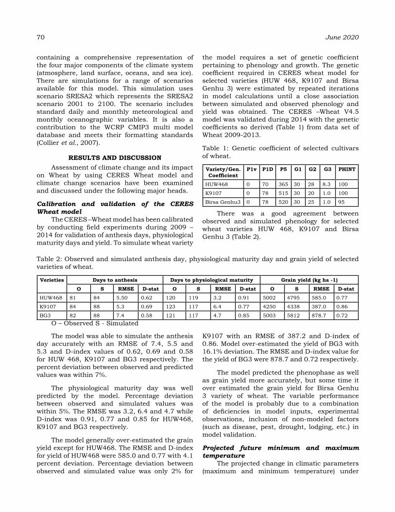
70 June 2020

containing a comprehensive representation of the four major components of the climate system (atmosphere, land surface, oceans, and sea ice). There are simulations for a range of scenarios available for this model. This simulation uses scenario SRESA2 which represents the SRESA2 scenario 2001 to 2100. The scenario includes standard daily and monthly meteorological and monthly oceanographic variables. It is also a contribution to the WCRP CMIP3 multi model database and meets their formatting standards (Collier et al., 2007).

reSuLtS aNd dISCuSSIoNAssessment of climate change and its impact

on Wheat by using CERES Wheat model and climate change scenarios have been examined and discussed under the following major heads.

Calibration and validation of the CERES Wheat model

The CERES –Wheat model has been calibrated by conducting field experiments during 2009 – 2014 for validation of anthesis days, physiological maturity days and yield. To simulate wheat variety

the model requires a set of genetic coefficient pertaining to phenology and growth. The genetic coefficient required in CERES wheat model for selected varieties (HUW 468, K9107 and Birsa Genhu 3) were estimated by repeated iterations in model calculations until a close association between simulated and observed phenology and yield was obtained. The CERES –Wheat V4.5 model was validated during 2014 with the genetic coefficients so derived (Table 1) from data set of Wheat 2009-2013.

Table 1: Genetic coefficient of selected cultivars of wheat.

variety/gen. Coefficient

P1v P1d P5 g1 g2 g3 PhINt

HUW468 0 70 365 30 28 8.3 100

K9107 0 78 515 30 20 1.0 100

Birsa Genhu3 0 78 520 30 25 1.0 95

There was a good agreement between observed and simulated phenology for selected wheat varieties HUW 468, K9107 and Birsa Genhu 3 (Table 2).

Table 2: Observed and simulated anthesis day, physiological maturity day and grain yield of selected varieties of wheat.

verieties days to anthesis days to physiological maturity grain yield (kg ha -1)

o S rMSe d-stat o S rMSe d-stat o S rMSe d-stat

HUW468 81 84 5.50 0.62 120 119 3.2 0.91 5002 4795 585.0 0.77

K9107 84 88 5.3 0.69 123 117 6.4 0.77 4250 4338 387.0 0.86

BG3 82 88 7.4 0.58 121 117 4.7 0.85 5003 5812 878.7 0.72O – Observed S - Simulated

The model was able to simulate the anthesis day accurately with an RMSE of 7.4, 5.5 and 5.3 and D-index values of 0.62, 0.69 and 0.58 for HUW 468, K9107 and BG3 respectively. The percent deviation between observed and predicted values was within 7%.

The physiological maturity day was well predicted by the model. Percentage deviation between observed and simulated values was within 5%. The RMSE was 3.2, 6.4 and 4.7 while D-index was 0.91, 0.77 and 0.85 for HUW468, K9107 and BG3 respectively.

The model generally over-estimated the grain yield except for HUW468. The RMSE and D-index for yield of HUW468 were 585.0 and 0.77 with 4.1 percent deviation. Percentage deviation between observed and simulated value was only 2% for

K9107 with an RMSE of 387.2 and D-index of 0.86. Model over-estimated the yield of BG3 with 16.1% deviation. The RMSE and D-index value for the yield of BG3 were 878.7 and 0.72 respectively.

The model predicted the phenophase as well as grain yield more accurately, but some time it over estimated the grain yield for Birsa Genhu 3 variety of wheat. The variable performance of the model is probably due to a combination of deficiencies in model inputs, experimental observations, inclusion of non-modeled factors (such as disease, pest, drought, lodging, etc.) in model validation.

Projected future minimum and maximum temperature

The projected change in climatic parameters (maximum and minimum temperature) under

different crop duration by two General Circulation Models (GCM) in year 2020, 2030, 2040 and 2050 are shown in table 3. In both the climate parameters, the change would be positive showing an increasing trend of maximum temperature and minimum temperature.

Average minimum and maximum temperature projected by both GCM showed (Table 3 & 4) that it would increase in coming decades during wheat growing season. Minimum temperature would be increased by 0.50 to 1.50 C in 2050 as compared to normal year (2010) as predicted by both GCM. Similarly maximum temperature is projected to increase by 0.20 to 10C in 2050. Increase in temperature would be more for minimum temperature as compared to maximum temperature.Grain yield of wheat was found negatively related with the temperature and

minimum temperaturerise being more detrimental than rise in maximum temperature (Kumari et al. 2017).

Impact of Climate change on WheatThe impact of climate change on agriculture

will become one of the major deciding factors influencing the future food security for mankind on earth. Agriculture is not only sensitive to climate change but, at the same time, is one of the major drivers for the climate change. Understanding the weather change over a period of time and adjusting the management practices towards achieving better harvest is a challenge to the growth of agricultural sector as a whole.

Impact on days to AnthesisThe simulated number of days to anthesis of

wheat in both GCM used for four periods of 2020,

Table 3: Minimum temperature pattern during crop duration under future climate change scenarios

variety Sowing

eChaM 5 CSIro MK3.5

2010 2020 2030 2040 2050 differ-ences

(2010-2050)

2020 2030 2040 2050 differences (2010-2050)

HUW 468

Normal 8.6 8.5 8.6 9.5 10 1.4 8.6 9 9.3 9.8 1.2

Mod. Normal 8.9 8.7 8.7 9.5 10 1.1 8.8 9.2 9.6 10 1.1

Late 10.1 9.4 9.5 10.2 10.7 0.6 9.4 9.9 10.1 10.6 0.5

K 9107

Normal 8.5 8.4 8.5 9.4 9.9 1.4 8.5 8.9 9.2 9.7 1.2

Mod. Normal 8.8 8.6 8.6 9.4 9.9 1.1 8.7 9.2 9.4 10 1.2

Late 10.0 9.2 9.3 10.0 10.6 0.6 9.4 9.7 10 10.5 0.5

Birsa Genhu 3

Normal 8.5 8.4 8.5 9.4 10 1.5 8.5 8.9 9.2 9.8 1.3

Mod. Normal 8.8 8.6 8.7 9.4 9.9 1.1 8.7 9.2 9.5 10 1.2

Late 10 9.2 9.3 10 10.6 0.6 9.4 9.7 10 10.5 0.5

Table 4: Maximum temperature pattern during crop duration under future climate change scenarios

variety Sowing eChaM 5 CSIro MK3.5

2010 2020 2030 2040 2050 differences (2010-2050)

2020 2030 2040 2050 differences (2010-2050)

HUW 468

Normal 25.3 25.6 25.6 25.9 26.3 1 25 25.1 25.2 25.5 0.2

Mod. Normal 26.3 26.6 26.6 26.9 27.2 0.9 25 25.2 25.2 26.5 0.2

Late 27.5 27.5 27.6 27.8 27.9 0.4 26.1 26.3 26.4 27.7 0.2

K 9107

Normal 25.1 25.5 25.5 25.9 25.9 0.8 24.9 25 25.1 25.4 0.3

Mod. Normal 26.2 26.5 26.5 26.9 26.9 0.7 25.9 26.1 26.1 26.4 0.2

Late 27.4 27.4 27.5 27.9 27.9 0.5 27 27.2 27.2 27.6 0.2

Birsa Genhu 3

Normal 25.1 25.5 25.6 25.9 25.8 0.7 24.9 25 25.1 25.4 0.3

Mod. Normal 26.2 26.5 26.6 26.9 26.8 0.6 25.9 26.1 26.2 26.4 0.4

Late 27.4 27.4 27.5 27.9 27.9 0.5 27 27.2 27.2 27.8 0.4


72 June 2020

2030, 2040, 2050 was less than the normal year (2010) of the studied region (Table 5). In other words, the prediction results of number of days to anthesis for future climate change showed that this phenophasic character will decrease under the situation of climate change. Predicted days to anthesis by both GCM showed a mixed trend (Table 5). It indicated an increase in number of anthesis days in 2020 and 2030 by 2 to 10 days for all selected varieties of wheat but it decreased during 2040 and 2050 by 1 to 10 days. Predicted reduction was more under ECHAM 5 as compared to MK 3.5 model. Among the varieties, Birsa Genhu 3 showed less variation in days to anthesis during coming decades as compared to current situation.

As stated, it is anticipated that the temperature will rise over the time that would lead

to the increase in evaporation and transpiration, leading to the increase in the growth rate of the plant. In other words the plant efforts to complete the growth process by recognizing the heat stress condition and as a result the period of planting to flowering is reduced. Also Roberts and Summerfield (2007) stated that the rise in temperature during the growth season leads to the fast growth and earlier flowering of the plant.

Impact on days to Physiological Maturity Model results also showed significant effect of

climate change on physiological maturity of wheat. The duration of physiological maturity has been predicated to decrease significantly due to change in climate. The number of days, from planting to maturity, also followed the similar trend of the number of days to anthesis. As in both models

Table 5:Simulation of days taken to Anthesis of wheat under future climate change scenarios using DSSAT model

variety Sowing eChaM 5 CSIro MK3.5

2010 2020 2030 2040 2050 differences (2010-2050)

2020 2030 2040 2050 differences (2010-2050)

HUW 468

Normal 85 83 83 78 76 9 87 85 83 81 6

Mod. Normal 82 84 84 80 77 5 87 85 84 82 5

Late 82 81 81 79 76 6 83 82 80 78 5

K 9107

Normal 90 88 88 83 80 10 92 90 88 86 6

Mod. Normal 86 89 88 84 82 4 92 90 88 86 6

Late 85 85 85 82 80 5 87 85 84 82 5

Birsa Genhu 3

Normal 89 88 88 83 80 9 89 92 90 88 6

Mod. Normal 87 89 88 84 82 5 92 92 90 88 4

Late 83 85 85 82 80 3 85 87 85 84 1

Table 6: Simulation of days taken to Maturity of wheat under future climate change scenarios using DSSAT model

variety Sowing

eChaM 5 CSIro MK3.5

2010 2020 2030 2040 2050 differences (2010-2050)

2020 2030 2040 2050 differences (2010-2050)

HUW 468

Normal 125 126 126 120 117 8 129 127 125 122 7

Mod. Normal 125 123 122 118 115 10 125 122 121 118 7

Late 115 117 117 114 111 4 118 116 115 112 6

K 9107

Normal 129 125 124 119 115 14 127 125 123 120 7

Mod. Normal 127 121 120 117 114 13 123 121 119 117 6

Late 117 115 115 112 109 8 117 114 113 110 7

Birsa Genhu 3

Normal 125 125 125 119 116 9 127 125 123 121 6

Mod. Normal 125 121 121 117 114 11 123 121 120 117 6

Late 115 115 115 112 109 6 117 114 113 110 7

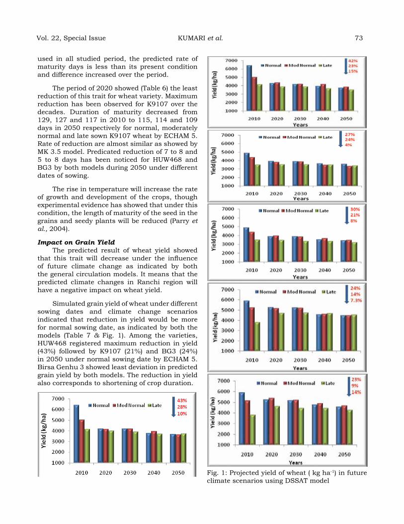
used in all studied period, the predicted rate of maturity days is less than its present condition and difference increased over the period.

The period of 2020 showed (Table 6) the least reduction of this trait for wheat variety. Maximum reduction has been observed for K9107 over the decades. Duration of maturity decreased from 129, 127 and 117 in 2010 to 115, 114 and 109 days in 2050 respectively for normal, moderately normal and late sown K9107 wheat by ECHAM 5. Rate of reduction are almost similar as showed by MK 3.5 model. Predicated reduction of 7 to 8 and 5 to 8 days has been noticed for HUW468 and BG3 by both models during 2050 under different dates of sowing.

The rise in temperature will increase the rate of growth and development of the crops, though experimental evidence has showed that under this condition, the length of maturity of the seed in the grains and seedy plants will be reduced (Parry et al., 2004).

Impact on Grain YieldThe predicted result of wheat yield showed

that this trait will decrease under the influence of future climate change as indicated by both the general circulation models. It means that the predicted climate changes in Ranchi region will have a negative impact on wheat yield.

Simulated grain yield of wheat under different sowing dates and climate change scenarios indicated that reduction in yield would be more for normal sowing date, as indicated by both the models (Table 7 & Fig. 1). Among the varieties, HUW468 registered maximum reduction in yield (43%) followed by K9107 (21%) and BG3 (24%) in 2050 under normal sowing date by ECHAM 5. Birsa Genhu 3 showed least deviation in predicted grain yield by both models. The reduction in yield also corresponds to shortening of crop duration.

Fig. 1: Projected yield of wheat ( kg ha-1) in future climate scenarios using DSSAT model


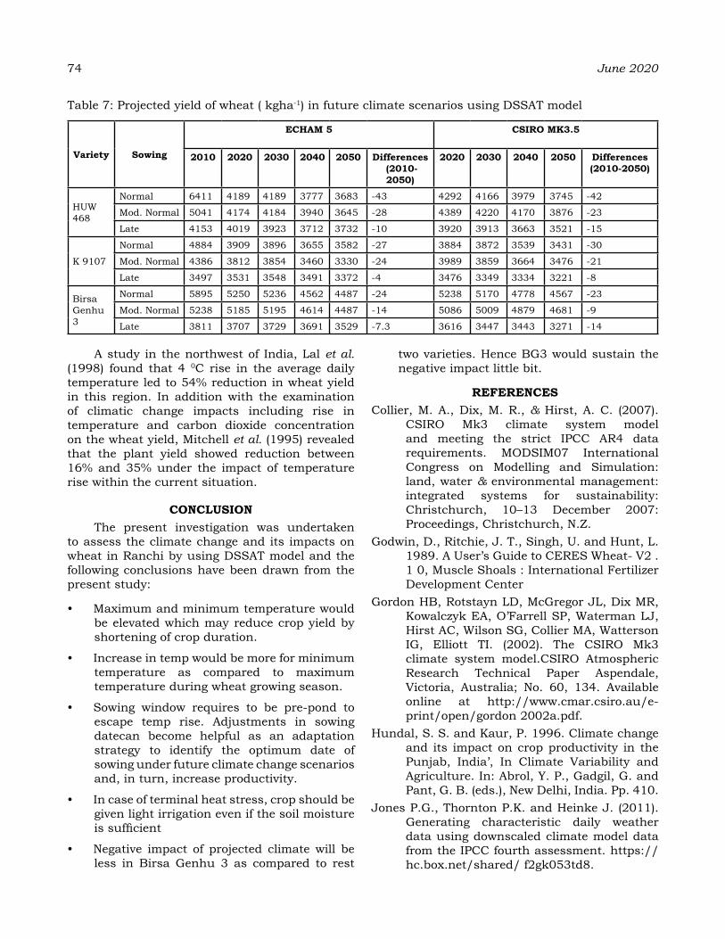
74 June 2020

A study in the northwest of India, Lal et al. (1998) found that 4 0C rise in the average daily temperature led to 54% reduction in wheat yield in this region. In addition with the examination of climatic change impacts including rise in temperature and carbon dioxide concentration on the wheat yield, Mitchell et al. (1995) revealed that the plant yield showed reduction between 16% and 35% under the impact of temperature rise within the current situation.

CoNCLuSIoNThe present investigation was undertaken

to assess the climate change and its impacts on wheat in Ranchi by using DSSAT model and the following conclusions have been drawn from the present study:

• Maximum and minimum temperature would be elevated which may reduce crop yield by shortening of crop duration.

• Increase in temp would be more for minimum temperature as compared to maximum temperature during wheat growing season.

• Sowing window requires to be pre-pond to escape temp rise. Adjustments in sowing datecan become helpful as an adaptation strategy to identify the optimum date of sowing under future climate change scenarios and, in turn, increase productivity.

• In case of terminal heat stress, crop should be given light irrigation even if the soil moisture is sufficient

• Negative impact of projected climate will be less in Birsa Genhu 3 as compared to rest

two varieties. Hence BG3 would sustain the negative impact little bit.

reFereNCeSCollier, M. A., Dix, M. R., & Hirst, A. C. (2007).

CSIRO Mk3 climate system model and meeting the strict IPCC AR4 data requirements. MODSIM07 International Congress on Modelling and Simulation: land, water & environmental management: integrated systems for sustainability: Christchurch, 10–13 December 2007: Proceedings, Christchurch, N.Z.

Godwin, D., Ritchie, J. T., Singh, U. and Hunt, L. 1989. A User’s Guide to CERES Wheat- V2 . 1 0, Muscle Shoals : International Fertilizer Development Center

Gordon HB, Rotstayn LD, McGregor JL, Dix MR, Kowalczyk EA, O’Farrell SP, Waterman LJ, Hirst AC, Wilson SG, Collier MA, Watterson IG, Elliott TI. (2002). The CSIRO Mk3 climate system model.CSIRO Atmospheric Research Technical Paper Aspendale, Victoria, Australia; No. 60, 134. Available online at http://www.cmar.csiro.au/e-print/open/gordon 2002a.pdf.

Hundal, S. S. and Kaur, P. 1996. Climate change and its impact on crop productivity in the Punjab, India’, In Climate Variability and Agriculture. In: Abrol, Y. P., Gadgil, G. and Pant, G. B. (eds.), New Delhi, India. Pp. 410.

Jones P.G., Thornton P.K. and Heinke J. (2011). Generating characteristic daily weather data using downscaled climate model data from the IPCC fourth assessment. https://hc.box.net/shared/ f2gk053td8.

Table 7: Projected yield of wheat ( kgha-1) in future climate scenarios using DSSAT model

variety Sowing

eChaM 5 CSIro MK3.5

2010 2020 2030 2040 2050 differences (2010-2050)

2020 2030 2040 2050 differences (2010-2050)

HUW 468

Normal 6411 4189 4189 3777 3683 -43 4292 4166 3979 3745 -42

Mod. Normal 5041 4174 4184 3940 3645 -28 4389 4220 4170 3876 -23

Late 4153 4019 3923 3712 3732 -10 3920 3913 3663 3521 -15

K 9107

Normal 4884 3909 3896 3655 3582 -27 3884 3872 3539 3431 -30

Mod. Normal 4386 3812 3854 3460 3330 -24 3989 3859 3664 3476 -21

Late 3497 3531 3548 3491 3372 -4 3476 3349 3334 3221 -8

Birsa Genhu 3

Normal 5895 5250 5236 4562 4487 -24 5238 5170 4778 4567 -23

Mod. Normal 5238 5185 5195 4614 4487 -14 5086 5009 4879 4681 -9

Late 3811 3707 3729 3691 3529 -7.3 3616 3447 3443 3271 -14

Kumar, S. Naresh,, Aggarwal, P. K. Swaroopa Rani, D. N. Saxena R., Chauhan, N.and Jain, S.2014. Vulnerability of wheat production to climatechange in India.Climate Research. 59: 173–187

Kumari, Pragyan ;Wadood, A; Singh, C.S. and Singh, S.K. (2017). Quantification of temperature and its effect on wheat yield in Jharkhand region. The Bioscan 12 (1) : 355- 358.

Lal, M., Singh, K. K., Srinivasan, G., Rathore, L. S. and Saseendran, A. S.: (1998), ‘Vulnerability of rice and wheat yields in NW-India to future change in climate’, Agric. Forest Meteorology 89, 101–114.

Mitchell, J. F. B., Johns, T. C., Gregory, J. M. and Tett, S. F. B.: (1995), ‘Climate response to increasing levels of greenhouse gases and sulphate aerosols’, Nature 376, 501–504.

Richter, O. and Sondgerdth, D., 1990, “Parameter estimation in ecology”, The link between data and models, VCH Publishers, Weinheim, FRG, p218.

Roberts, E.H. and Sommerfield, R.J.: (2007), Measurement and prediction of flowering in annual crops, Manipulation of Flowering, Butterworths, London, pp. 17-50.

Roeckner, A., Brokopf, R., Esch, M., (2003). The atmospheric general circulation model ECHAM5. Part I: model description. MPI Report 349. Hamburg:Max Planck Institute for Meteorology. 127 pp.

Roeckner, E., Arpe, K., Bengtsson, L., Brinkop, S., Dümenil, L., Esch, M., Kirk, E., Lunkeit, F., Ponater, M., Rockel, B., Suasen, R., Schlese, U., Schubert, S. and Windelband, M. (1992). Simulation of the present-day climate with the ECHAM4 model: impact of model physics and resolution. Max-Planck Institute for Meteorology, Report No. 93, Hamburg, Germany, 171pp.

Roeckner, E., Arpe, K., Bengtsson, L., Christoph, M., Claussen, M., Dümenil, L., Esch, M., Giorgetta, M., Schlese, U. and Schulzweida, U. (1996). The atmospheric general circulationmodel ECHAM-4: model description and simulation of present-day climate. Max-Planck Institute for Meteorology, Report No. 218, Hamburg, Germany, 90pp.

Saini, A. D. and Nanda, R.: 1986. Influence of temperature and light intensity during early growth period on grain number in wheat. Indian Journal of Agricultural Sciences 56: 512-519.

Willmott, C. J. (1982). Some comments on the evaluation of model performance. Bulletin of the American Meteorological Society, 63, 1309–1313.

Willmott, C. J., Ackleson, S. G., Davis, R. E., Feddema, J. J., Klink, K. M., Legates, D. R., O’Donnell, J., & Rowe, C. M. (1985). Statistics for the evaluation of model performance.Journal of Geophysical Research, 90 (C5), 8995–9005.


Weather based decision support system for crop risk management

M.L. KhIChar*, raM NIWaS, aNIL KuMar, raJ SINgh aNd S.C. BhaN1

Department of Agricultural MeteorologyCCS Haryana Agricultural University Hisar 125004 India

1India Meteorological Department (IMD), New Delhi *Corresponding author E-mail id: [email protected]

aBStraCtChaudhary Charan Singh Haryana Agricultural University in collaboration with India Meteorological Department, Ministry of Earth Sciences, GoI has been rendering weather forecast based Agromet Advisory Service (AAS) for benefit of farmers in the state through Agromet Field Units (AMFU) on Tuesday and Friday for next five days. Farmers of Haryana have begun to adopt new technologies and practices in recent years to become more and more climate smart for better economic returns without much external support. The weather based information was disseminated through several modes of communication viz. radio, television, local and regional newspapers, toll free numbers, community radios, etc., to the farmers of the Haryana state. The use of aforesaid means of dissemination of agromet advisory to the farmers have limitation i.e. less lead time is available for day to day planning for agricultural operations in the field. Web enabled agromet information system www.emausamhau.gov.in and www.emausamhau.com were developed for real time dissemination of agromet advisory to the farmers of the state under climate smart agriculture has the advantage of increase in lead time by reducing time in dissemination. It is a system that support the weather based farm decision making activities to the farmers through SMSs, mobile App and information kiosk. It provides real time weather based agro-advisory and benefit in managing the farm operations and reducing input losses. The weather based crop advisory services helped the farmers for maximize profit by increasing farm production and minimizing weather related losses. The Adaptive capacity of the farming community has been strengthened through reduced cost of cultivation and input use, access to knowledge, information and technology, and reduced risk from drought and other extreme events. In the current status >3.5 lakh farmers across the state have been receiving the weather based farm information through real time agromet decision support system for crop risk management through web enabled SMS services. The farmers showed overwhelmed response for their registration under mobile SMS and download the mobile app emausamhau from Google play store for weather forecast based crop information. It will help to enhance the farm productivity and farmer’s income to be doubled by reducing farm losses with timely guidance through decision support system.

Keywords: Advisory, climate, weather, agromet advisory services, real time, mobile App, SMS

INtroduCtIoN

Agriculture and an area of human activity with are at risk from climate change as well as a driver of climate and environmental change, features prominently in the global climate change agenda. To alleviate some of the complex challenges posed by climate change, agriculture (including forestry and fisheries) has to become “climate smart”, that is, sustainably raise agricultural productivity and incomes, adapt and build resilience to climate change, and reduce greenhouse gases emissions, where possible (FAO, 2013a). Climate-smart agriculture is defined as an approach for transforming and reorienting agricultural development under the new realities of climate change (Lipper et al., 2014).

Climate change is the most serious ecological

risk to fight against hunger, malnutrition, disease and poverty in world. Agriculture is the most susceptible and sensitive sector affected by climate change because of its dependency on local climate parameters like rainfall, temperature, soil health etc. To alleviate the challenges posed by climate change, agriculture has to become “climate smart”, that is, sustainably increase agricultural productivity and incomes, adapt and build resilience to climate change, and reduce or remove greenhouse gases emissions, wherever possible. Despite the recognized importance of Climate-Smart Agriculture (CSA), the dissemination and uptake of climate-smart technologies, tools and practices is still largely an ongoing and challenging process. The adaption of climate-related knowledge, technologies and practices to local conditions, promoting joint learning by


farmers, researchers, extension worker and widely disseminating CSA practices, is serious issue. There is a need for site-specific assessments to identify suitable agricultural technologies and practices needed for CSA. Disseminating climate information and sharing agricultural information can be facilitated by application made available through Information Technology by using weather based decision support system. Agro Advisory Services contribute towards Climate Smart Agriculture by disseminating climate information and technologies on production practices for climate adaption through innovative approaches, such as climate-smart villages, climate trainings or workshops, etc.

Weather forecast is becoming more important task for efficient management of farm inputs. The accuracy of forecast for a long period is a great challenge, but the medium range weather forecasts in recent year were improved to a great extent due to modern technology. Furthermore, web-based decision support system has been developed and used to disseminate agricultural information. This study, therefore, investigates weather based decision support systems with SMS system that farmers and agricultural extension workers can operate, understand and access to agricultural information, especially climate information and innovations and to support strategic farm decisions under a changing climate.

MaterIaLS aNd MethodSThe District wise crop specific advisories

on the basis of prevailing crop situation and anticipated weather condition in consultancy with other extension subject specialists were uploaded online in weather based decision support system for crop risk management in Haryana State. The design and development of web enabled decision support system consists smart mobile emausamhau App (https://play.google.com/store/apps/details?id=com.emosumhisar.hau & hl=en_IN) and online farmer’ registration and message service system emausamhau.gov.in developed with help of National Information Center (NIC) through step wise information and suggestion under the supervision of Department of Agricultural Meteorology, CCS HAU, Hisar. Further, daily updating the other weather and crop inputs, which dynamically as require and needed over the server website/page and parallel looking the version (V) up-gradation with the new future in the software, point of consideration. The crop

specific package and practices/ recommendation of University followed and uploaded on the web enabled system. Also weather forecast, satellite and radar products and other weather based information regularly or dynamically updating or retrieving from India Meteorological Department (IMD)’ website. Online solution of query of the farmers regarding weather, insect pest disease crop management was developed in Emausamhau mobile app.

reSuLtS aNd dISCuSSIoNWeather Information & Agro-Advisory Agromet Advisory Service System

The AAB is usually prepared based on location specific forecasting system which has eight different weather parameters (rainfall (Rf), maximum temperature (Tmax), minimum temperature (Tmin), wind direction (WD), wind speed (WS), cloud cover (CC), morning relative humidity (RHm) and evening relative humidity, RHe). It also contains information relating to the crop cultivation namely, field preparation, sowing, irrigation, time and method of fertilizer and pesticide application, etc., in relation to weather forecast. Livestock management information regarding housing, animal health, feeding, nutrition and vaccination are also provided to the farmers through AAB with the consultation of Scientists of sister Institute LUVAS. The identification of appropriate breeds, nutrition and feeding considerations. Disease control measures, general care- necessary protection from heat, cold, wind etc. It helps for taking suitable measures to minimize the ill effect due to weather. AABs are being prepared twice in a week with the help of district and block level weather forecast received from India Meteorological Department. The bulletins prognosticate 5-days in advance which is also very helpful to the farming community to take necessary action in advance at time of crop cultivation. AAB is the best tool for transferring agro techniques and location specific recommendation of State Agricultural University to the end users. The agricultural productions are generally attributed to the behaviour of weather (space & time). It also provides, mitigation techniques on vulnerable information about crop management practices viz., irrigation scheduling, pest and diseases status and control management, livestock production and management, marketing and trade management, new scientific storage and processing information to the farmers (Rathore et al., 2004). Similarly, Rao et al., (2008) and

Vol. 22, Special Issue KHICHAR et al. 77

78 June 2020

Jaybhaye et al., (2018) reported that the weather based AAB on medium range weather forecast is used to minimize the risk from weather and weather induced pest and diseases. The existing methods of dissemination include radio, television, local and regional newspapers, toll free numbers, community radios and electronic mail. The use of aforesaid means of dissemination of agromet advisory to the farmers have limitation i.e. less lead time is available for day to day planning for agricultural operations in the field. But now farmers began to adopt new technologies and practices to become more and more climate smart for better economic returns. Web enabled agrimet information system www.emausamhau.gov.in and www.emausamhau.com were developed for real time dissemination of agromet advisory to the farmers of the state under climate smart agriculture has the advantage of increase in lead time by reducing time in dissemination.

Effective weather and climate information and advisory services help in decision-making of farmers and improve their management of related agricultural risks. Such agro-advisory services help to develop sustainable and economically viable agricultural systems, improve production and quality, reduce losses and risks, decrease costs, increase efficiency in the use of water, labour and energy, conserve natural resources, and decrease pollution by agricultural chemicals or other agents that contribute to the degradation of the environment. These Services meet the real-time needs of farmers and contribute to weather-based crop/livestock management strategies and operations dedicated to enhancing crop production and food security. This service aims at providing disaggregated district/block level information of

each agro-ecological sub-region’s weather, agro-met advisory, SMS alerts for weather forecast and crop impact and grievance management through multiple service delivery channels to the farmers.

Decision Support SystemWeb enabled decision Support System is

the collection of integrated software applications in the form of stepwise decision making process. The system assists management decision making by combining data, sophisticated analytical tools and user-friendly software into a single powerful web enabled system that can support structured, unstructured and semi structured decision making. Weather based Decision Support System is an online computer-based information system, which provides observed and moderated weather forecasted information to experts. Further experts prepares advisory and recommendation for crop risk management on the basis of weather forecast and bulletins, short messages are being disseminated through web based (http://www.emausamhau.com/) SMS/ Mobile App/Social Media, print media etc. It is a system that support the weather based farm decision making activities to the farmers through SMSs, mobile App and information kiosk. It provides real time weather based agro-advisory and benefit in managing the farm operations and reducing input losses.

Online Farmer Solution SystemOnline farmer solution system is available

in the mobile app Emausamhau. In this system farmers submit the photo of affected plant with query on the server thereafter the query forwarded to the concerned experts. Experts provide the solution of the query and send to the concerned farmers through web enabled decision support system. The system helps to manage the insect pest disease and day to day field work to the farmers.

Online feedback monitoring system:

The regular feedback has been collected from registered farmers by web enabled decision system. The feedbacks exhibited that most of the farmers are aware of agromet advisory services and rated as beneficial. Majority of the farmers want timely out reach of agromet advisories in the form of SMS in their mobiles. They demand an accurate extended range forecast and accuracy should be further increased. Farmers want accurate quantitative and region-specific (block level) rain forecast in future. The opinion of Users/Farmers regarding weather forecast are very responsive and very useful for application of pesticides and other day to day management practices. The adaptation measures for crop disease forecasting from the present studies found that nearly 72 % farmers believe that weather affect the crop health or growth. Among the adopters, 67-74 percent farmers use weather based advisory for managing their crop disease and insect-pest. Approximately 76 percent farmers had responded that they are using weather-based AAS for scheduling irrigation in field. Accurate and timely weather forecast is necessary for proper crop management. The different statistical, crop growth simulation and other methods have been developed for crop yield forecasting which take in to consideration the influence of weather and technological advances on crop yield. Study implies that crop-related issues were found to have significant relationship with the adaptation of farmers. Rainfall forecast is useful for saving the input water, irrigation scheduling as well as pesticides losses. Day to day crop management can be done with the help of weather forecast and weather based agromet advisories. Monsoon forecast is useful for

selecting the sowing time, variety, crop and area for particular crop. These AAB helps farmers to know the latest technologies which are a good sign that speaks about the interest of the farmers.

CoNCLuSIoNWeb enabled decision support system

helped in encouraging the adoption and use of modern crop production technologies and practices, in promoting weather-based irrigation management, pest/disease management, post-harvest technologies and commercial marketing of commodities etc. The web enabled based agromet advisory services improved production and productivity of the farming community. This may be attributed to less input capital, save the irrigation water and mitigate the problems of pests and diseases by using real tome weather based agro-advisory decision support system.

reFereNCeSFAO, (2013a). Sourcebook on Climate Smart

Agriculture, Forestry and Fisheries, Food and Agriculture Organisation of the United Nations (FAO), Rome, Italy. Retrieved from http://www.fao.org/ climatechange/37491-0c425f2caa2f5e6f3b9162d39c8507fa3.pdf

Jaybhaye, P.R., N.H. Deore and Shinde, P.B. (2018). Agromet Advisory Bulletin - A Weather Smart Agriculture Technology option for Adaptation and Mitigation of Changing Climate. Int. J. Curr. Microbiol.App. Sci., 7 (02) : 2644-2653.

Lipper, L., Thornton, P., Campbell, B.M. and Torquebiau, E.F. (2014). Climate –smart agriculture for food security. Nature Climate Change 4: 1068-1072. Retrieved from http://dx.doi.org/10.1038/ nclimate2437

Rao, A.S., (2008). Weather based agro advisory service for food security in the Indian and region. J. Agrometeorol., (SI-II) : 535- 540.

Rathore, L.S., Singh, K.K., and Gupta, A., (2004). National Centre for Medium Range Weather Forcasting: Activities, current status and future plans. J. Agrometeorol., 6: 258-264.

Vol. 22, Special Issue KHICHAR et al. 79

Weather based yield prediction model at various growth stages of wheat crop in different agro Climatic Zones of Jammu region

MaheNder SINgh, Charu SharMa, B.C. SharMa, vIShaW vIKaS aNd PrIYaNKa SINgh1

Agrometeorology Section, Division of AgronomySher-e-Kashmir University of Agricultural Sciences & Technology of Jammu

Main Campus, Chatha, Jammu-180009 (J & K), 1AAS Division, India Meteorlogical Division, Lodi Road, New Delhi-110003


aBStraCtLong term seed yield and weather data during growing period of wheat crop from 1991 to 2012 was collected from different offices or agencies for development of the district level yield forecast models. Further, the field experiments at research farm of Agrometeorology Section of SKUAST-J, Chatha, Jammu were also conducted in order to validate these models during rabi season of 2012-13 and 2013-14. Pre harvest yield prediction models for wheat crop has been prepared for different districts of Jammu region using this data. For the prediction of wheat seed yield at F2 stage, the long period weather data from 46th to 5th standard meteorological week (SMW) from 1991 to 2012 were used, where as at F3 stage, the data used from 46th to 9th standard meteorological week. The statistical weather based models for prediction of wheat yield for five districts of Jammu region were developed using the long term data. Models were validated with 2 years (2013 and 2014) data. For developing the yield forecast, models using composite weather variables have been studied. Simple and weighted weather indices have been prepared for individual weather variables as well as for interaction of two at a time considering throughout the crop growing season. The prediction models were able to explain the inter annual variation in the seed yield of wheat to an extent of 78, 74, 70, 73 and 68 percent and 82, 75, 76, 80 and 77 percent for Jammu, Kathua, Kishtwar, Udhampur and Doda districts during rabi 2012-13 and 2013-14, respectively. The validation results indicate that prediction of yield forecast is better for most of the Districts in 2014 as compared to 2013. The predicted rabi wheat yields for most of districts are within acceptable error limit (± 10 percent) in both the years of validation.

Keywords: Wheat, prediction model, weather, districts, seed yield, stages, Jammu region.

INtroduCtIoN

Reliable yield forecasting within the growing season would enable proper planning and more efficient management of grain production, handling, and marketing. The pre harvest crop yield prediction is also required for policy decisions like storage, pricing, marketing, import, export etc. Weather is the main component that influence yield of crop. Weather based on crop models can provide reliable forecast of crop yield in advance of harvest and also forewarning of pests and diseases attack so that suitable plant protection measures could be taken up timely to protect the crops (Agrawal and Mehta, 2007). Therefore model based on weather parameters can provide reliable forecast in advance for crop seed yield. Weather indices based regression models was found to be better in some cases whereas in some cases reverse trend was found (Chandrahas et al., 2010). Forecasting Agricultural output

using Space, Agro meteorology and Land based observations (FASAL) is an important project operational at Ministry of Agriculture, Govt. of India in collaboration with Space Application Centre (SAC), Institute of Economic Growth (IEG) and India Meteorological Department (IMD). Under this FASAL project, IMD in collaboration with 46 Agromet Field Units (AMFU) located at different parts of the country develops intra-seasonal operational yield forecast at district and state level for 13 major crops of India during kharif and rabi seasons using statistical model (Ghosh et al., 2014). The mandate of this project is to issue multiple crop yield forecast for various major crops under different agro-climatic zones of the states at initial stage (F1), mid-season (F2) and pre-harvest (F3) stages.

Wheat (Triticum aestivum L.) occupying second place in production and plays an important role in food security of India. In India, the total


area under wheat crop is about 30.97 million hectares with production of 88.74 million tons and productivity of 2872.0 kg/ha during the year 2014-15 (Anonymous, 2015). Therefore forecasting of wheat yield is important for economic planning by policy makers in the government. Therefore, the study has been undertaken to develop the model for wheat by analyzing the weather variables using past weather and yield records of different districts of Jammu region so that, a long series could be obtained in a shorter time.

MaterIaLS aNd MethodLong term seed yield were collected from

Department of Economics and Statistics, Government of Jammu and Kashmir and weather data collected from India Jammu Meteorological Department, Pune of different districts from 1991-2012. The geographical locations of different district (Jammu, Doda, Kishtwar, Kathua and Udhampur) located at different agro climatic zone of Jammu region are presented in Table 1. The daily weather data were used for calculating weekly as well as the corresponding months in which the particular growth stage of the crop lies except the harvesting period were used to develop the district level yield forecast models. The standard meteorological week (SMW) wise weather data from 46th to 5th were used to develop weather based yield prediction regression models for F2 (pre flowering or spike emergence) stage and 46th to 13th for F3 (pre harvesting or dough) stage

of wheat crop for above said five districts. The variable used in the study were maximum (Tmax) temperature (ºC), minimum (Tmin) temperature (ºC), morning relative humidity (RH I, percent), afternoon relative humidity (RH II, percent) and rainfall (RF, mm). Different weather indices were generated using weekly values of weather parameters and their weighted values using correlation coefficient and presented in Table 2. To study the combined effects of weather variables on wheat seed yield, the model used for studying effect of individual weather variables had also been extended by including interaction terms as per the IASRI, New Delhi suggested by Hendricks and Scholl, 1943. Further, modified by Agrawal et al. 1980; 1983; Jain et al., 1980 for expressing effects of changes in weather variables on yield in the successive periods as second degree polynomial in respective correlation coefficients between yield and weather variables. The modified model used in the present study and for developing district wise yield prediction equations for wheat crop are as under:

Where

Table 1: Geographical locations of different districts of Jammu region.

aCZ Sub-tropical low altitude

Intermediate temperate high altitude

Districts Jammu Kathua Udhampur Doda KishtwarLatitude (ºN) 32.73 32.17 32.55 33.13 33.19Longitude (ºE ) 74.52 75.36 75.09 75.57 75.48Altitude (m) 308 320 742 1144 1627

Table 2: Weather derived indices used in models using composite weather variables.

Weather Parameters

Simple weather indices Weighted weather indices

tmax tmin rF rhI rhII tmax tmin rF rhI rhII Tmax Z10 Z11 Tmin Z120 Z20 Z121 Z21 RF Z130 Z230 Z30 Z131 Z231 Z31 RHI Z140 Z240 Z340 Z40 Z141 Z241 Z341 Z41 RHII Z150 Z250 Z350 Z450 Z50 Z151 Z251 Z351 Z451 Z51


82 June 2020

Where,

Y = variable to forecast or seed yield of wheat

Xiw/Xii’ww is the value of ith/i’th weather variable under study in wth week,

riw/rii’w is correlation coefficient of yield with ith weather variable/product of ith and i’th weather variables in with week, respectively.

m is the week of forecast

p is the number of weather variables used and c is the random error distribution as N (0, σ2).

In this model, two weather indices were developed for each weather variable, i.e. simple (unweighted index- Zi0) as well as weighted (weighted index- Zi1) accumulation of weekly weather variable, weights being correlation coefficients of weather variable in respective weeks with yield. Similarly, indices were also generated for interaction of weather variables, using weekly products of weather variables taking two at a time. Combination of weather variables for weather indices, thus, generated are presented in table 2. Regression analysis was used for fitting equation taking yield as dependent variable and considering year and weather as independent variable using the SPSS software. Weather scores for each year at different phases of crop growth obtained through these discriminant functions were used along with inputs and time trend as regressors in model development through stepwise regression. The weighting coefficients in these equations are by necessity obtained in an empirical manner using standard statistical procedures, such as multivariable regression analysis. For the validation of the above said prediction model, field experiments were conducted at research farm of Agro meteorology Section, of SKUAST-J, Chatha, Jammu during rabi season of 2012-13 and 2013-14. The experiments consist of three sowing environments/dates, in which most of the sowing of wheat was done in the area with three most common varieties of the region. The experiment was conducted in randomized block design with three replication.

reSuLtS aNd dISCuSSIoNStatistical wheat forecast models during pre-

flowering and pre-harvesting were developed for a 22 years of datasets and validated for years 2012-13 and 2013-14. The seed yield prediction models of rabi wheat for different districts of Jammu

Province have been prepared by using standard statistical procedures, such as multivariable regression analysis. The weather based yield prediction model for wheat developed with coefficient of determination (R2) at pre-flowering (F2) and pre-harvesting (F3) stage and presented in Table 3. Coefficient of determination (R2) was significant at 5 percent of confidence level in all the five districts of Jammu province. The R2 was ranged between 0.69 (Udhampur) and 0.81 (Jammu) at F2 (pre flowering) stage and ranged between 0.74 (Kathua) and 0.85 (Jammu) at F3 (pre harvesting) stage (Table 3). The accuracy at F3 stage for prediction of wheat seed yield was found appropriate stage for all the five districts and similar types of results were reported by Baier, 1977.

The best agro meteorological indices to incorporate in the agro meteorological yield forecast model at pre flowering stage was found effective contributor as RH I (Z 40), RH I (Z 41), Tmax X RH I (Z 141), Tmax X RH II (Z151) and Tmin X RH II (Z 250) for Jammu, RH II (Z51) for Kathua, T min (Z21), Tmin X RF (Z231) and RF X RH I (Z341) for Udhampur, T max (Z11), RF (Z31) and RH I X RH II (Z450) for Doda, Tmax X RH II (Z151) and Tmin X RF (Z231) for Kishtwar. At pre harvesting stage (F3), the best agrometeorological indices were selected as RH I (Z40 and Z41) for Jammu, T max X RF (Z131) and Tmax X RH II (Z151) for Kathua, Tmin (Z21) and RF X RH I (Z341) for Udhampur, Tmax (Z11) and RH I (Z41) for Doda and Tmax (Z11) and Tmax X RH II (Z151) for Kishtwar district (Table 3).Theresults were also reported by Patel el al., 2018 has also conducted a study to develop regression model for Bilaspur districts of Chhattisgarh.The relative humidity (morning & evening) and temperature (minimum & maximum) were found most appropriate weather parameters for prediction of wheat seed yield under various agro climatic conditions of Jammu region. Such types of results were also reported by Rakhee et al., 2018 for prediction of rice yield of Kanpur district.

The validation of model also done with the results of experiments conducted as well as the actual yield of wheat crop observed at these locations during 2012-13 and 2013-14 and presented in Table 4. Results revealed that the model overestimated the seed yield of wheat at Doda by 9.9 percent, Kishtwar (4.8 percent), Kathua (2.5 percent) and underestimated at Jammu by 0.1 percent and Udhampur (10.5

percent) at pre flowering (F2) Stage during rabi 2012-13 (table 4). Whereas, it underestimated for the same stage by 7.9 to 12.5 percent variations at all the locations except Kishtwar during rabi 2013-14, it might be due the variation in weather parameters at different growth period of the crop. Similar findings was also reported by Chandrahas et al., 2010.

The prediction at pre harvesting (F3) stage by these model overestimated of seed yield at Jammu, Doda, Kishtwar. Kathua by 6.6. 5.7, 9.0, 1.1 percent variation, respectively and underestimated by 11.5 percent at Udhampur during 2012-13. Whereas, these modelswere underestimated the seed yield of wheat by 9.7, 19.3, 10.2 percent variation at Jammu, Kathua Udhampur, respectively andoverestimated by 2.4, 4.0 at Doda and Kishtwar districts during rabi2013-14, respectively (table 4). This may due fluctuations in temperature and relative humidity at these location during 2012-13 as compared to 2013-14. Impotence of change in temperature in

wheat growing areas of India has been highlighted by Sandhu et al. 2016.

The results indicate that model has predicted seed yield of wheat crop during rabiseason for most of the districts were found within acceptable error/ variation limit (±10 percent) in both the year of validation study. However, prediction was marginally lower only for Kathua and Udhampur districts. Temperatures (Maximum and minimum) and relative humidity (morning and evening) were found most important agrometeorological indices for wheat seed yield prediction at various agro climatic zones of Jammu region. Predicted yield was very closer to observed yield, therefore it suggested that these prediction models can be used for yield forecasting and planning purpose in the region. The results showed that agro-meteorological yield model explained the yield variability due to variations in minimum and maximum temperatures together with relative humidity with respect to major wheat growing districts of Jammu Province. According to Lalet

Table 3: Yield prediction model at F2 and F3 stages of wheat crop for different districts of Jammu region.

S.No. district Stage equation R2

1 Jammu

F2 -13.0198 - 0.06*Z40 + 0.35*Z41 + 0.003 *Z141 + 0.0050*Z151 – 0.0011*Z250

0.81

F3 -7.77 – 0.0245*Z40 + 0.239*Z41 0.852

KathuaF2 6.47 + 0.035*Z51 0.79 F3 9.62 + 0.0021*Z131 + 0.0020*Z151 0.74

3 Udhampur

F2 20.32 + 0.4300*Z21 + 0.0051*Z231 + 0.0008*Z341 0.69 F3 22.27 + 0.31*Z21 + 0.0002*Z341 0.75

4 Doda

F2 26.52 + 0.352*Z11 + 0.034*Z31 -0.00003*Z450 0.78 F3 23.65 + 0.1587*Z11 – 0.0562*Z41 0.82

5 Kishtwar

F2 2.28 + 0.095*Time + 0.0315*Z151 + 0.016*Z231 0.74 F3 14.11 - 0.0741*Time + 0.1420*Z11 + 0.0008*Z151 0.77

Table 4: Observed and forecasted wheat yield (kgha-1) at F2 and F3 Stage of various districts of Jammu Province duringrabi2013 and 2014.

Year Jammu Kathua udhampur doda KishtwarObserved seed yield (kg/ha)

2013 1811 1537 1606 1129 12372014 2406 2129 1701 1129 1169

Forecasted yield at F2 stage (kg/ha)

2013 1810 (0.1) 1577 (-2.5) 1453 (10.5) 1253 (-9.9) 1299 (-4.8) 2014 2177 (10.5) 1893 (12.5) 1551 (9.7) 1046 (7.9) 1228 (-4.8)

Forecasted yield at F3 stage (kg/ha)

2013 1940 (-6.6) 1630 (-5.7) 1440 (11.5) 1240 (-9.0) 1251 (-1.1) 2014 2194 (9.7) 1784 (19.3) 1543 (10.2) 1157 (-2.4) 1218 (-4.0)

The value in parenthesis are variation/error (±) in the seed yield (percentage)


84 June 2020

al., 1998, Maximum and minimum temperatures are very sensitive weather parameters for wheat crop, a rise by 0.5°C in winter temperature is projected to reduce wheat yield by 0.45 t ha-1 in India. Wheat growing belts of this region are also largely influenced by maximum and minimum temperatures prevailed during the cropping season. We, therefore in fer that maximum and minimum temperatures together with RH were significant weather parameters for deciding wheat productivity in the region. The results revealed that reliable forecasts can be obtained using this approach when the crops are 10-12 weeks old. However, these studies were carried out at district level and required a long series data of 25-30 years which are not available for most of the locations.

CoNCLuSIoNTemperatures (maximum and minimum)

and relative humidity (morning and evening) were found most important agro meteorological indices for wheat seed yield prediction at various agro climatic zones of Jammu region. The pre harvested seed yield prediction by developed models can be reasonably accurate with R2 (between 0.69 and 0.85). These models were validated with ±10 percent variation for all the five districts of Jammu region. The performance of the model in predicting yield at district level for wheat crop is quite satisfactory. Therefore, it could be used for wheat yield forecasting for all the five districts of Jammu Province. These models were used to forecast yield of wheat in different situations, viz; (i) rain fed area having deficient rainfall (rice), (ii) rainfed area having adequate rainfall (rice) and (iii) irrigated area (wheat).

reFereNCeSAgrawal, R., Jain, R.C., Jha, M.P. and Singh,

D. (1980). Forecasting of rice yield using climatic variables. Ind.J. Agri. Sci. 50 (9) : 680-84.

Agrawal, R., Jain, R.C. and Jha, M.P. (1983). Joint effects of weather variables on rice yield. Mausam, 34 (2) :189-94.

Agrawal, R. and Mehta, S.C. (2007). Weather based forecasting of crop yields, pests and diseases- IASRI- Models. J. Ind. Soc. Agril.Stat., 61 (2) :255-263.

Anonymous, (2015). Agricultural Statistics at

a glance 2015. Directorate of Economics & Statistics, Department of Agriculture, Cooperation & Farmers’ Welfare, Government of India, New Delhi, http://eands .dacne t .n i c . in/Agr i cu l tu ra l _Statistics_At.Glance-2015%20Ebook/book.

Baier, W. (1977). Crop weather models and their use in yield assessments. Tech. note no. 151, WMO, Geneva, 48 pp.

Chandrahas, Agrawal, R. and Walia, S.S. (2010). Use of discriminant function and principal component techniques for weather based crop yield forecasts. (IASRI, New Delhi).

Ghosh, K., Balasubramanian, R., Bandopadhyay, S., Chattopadhyay, N., Singh, K.K. and Rathore, L.S. (2014). Development of crop yield forecast models under FASAL-a case study of kharif rice in West Bengal. J. Agrometeorol., 16 (1) : 1-8.

Hendrick, W.A. and Scholl, J.C. (1943). Technique in measuring joint relationship. The joint effects of temperature and precipitation on crop yield. N. Carolina Agric. Exp. Stat. Tech. Bull. 74.

Jain, R.C.; Agrawal, R. and Jha, M.P. (1980). Effects of climatic variables on rice yield and its forecast. Mausam. 31 (4) : 591-96.

Lal, M., Singh, K.K., Rathore, L.S., Srinivasan, G. and Saseendran, S.A. (1998). Vulnerability of rice and wheat yields in NW India to future changes in climate. Agric. For. Meteorol., 89: 101-114.

Patel A., Yadu, A., Gautam, S. and Rawat, S. (2018). Multivariate statistical wheat yield prediction model for Bilaspur district of Chhattisgarh.Int. J. of Chem. St.: 6 (6) : 2777-2781

Rakhee, Singh, A. and Kumar, A. 2018. Weather based fuzzy regression models for prediction of rice yield. J. Agrometeorol. 20 (4) : 297-301.

Sandhu, S.S., Prabhjyot-Kaur, Tripathi, P., Patel, S.R., Prasad, R., Solanki, N.S., Kumar, R., Singh, C.B., Dubey, A.P. and Rao, V.U.M. (2016). Effect of rise in intra seasonal temperature at major wheat growing locations in India: A study using CERES-Wheat model. J. Agrometeorol. 18 (2) : 222-233.

evaluation of actual evapotranspiration, water surplus and water deficit for climate smart rainfed crop planning in Bihar

aBduS Sattar1, S.a. KhaN2 aNd guLaB SINgh1

1Centre for Advance Studies on Climate Change, Dr. Rajendra Prasad Central Agricultural University, Pusa, Samastipur, Bihar-848 125

2Department of Agril. Meteorology & Physics, Bidhan Chandra Krishi Viswavidyalaya, Mohanpur, Nadia, West Bengal-741252


aBStraCtAgroclimatic study was carried out for the state of Bihar to evaluate actual evapo-transpiration (AET), water surplus (WS) and water deficit (WD) during different seasons viz. kharif, rabi and summer. Thematic maps comprising AET, WS and WD were generated to assess seasonal water use, water surplus and water deficit (high, moderate and low) zones in different districts of Bihar for developing climate smart crop production strategies for rainfed ecosystem. The AET, WD and WS were estimated through climatic water balance method based on historical rainfall data (30-55 years) of 110 rain-gauge stations, normal weekly potential evapotranspiration (PET) and available water holding capacity (AWC) of coarse-, medium- and fine-textured soils. The results revealed that maximum annual AET >800 mm was recorded in Kishanganj, major parts of Araria, Madhepura and Bhagalpur districts and in a small pocket in West Champaran district. The lowest annual AET (<600 mm) was recorded in some pockets of Nalanda district due to low AWC and rainfall. Major parts of Bihar exhibited the annual AET ranging from 600 to 800 mm during kharif season. While considering WS, the districts under Zone II (North-east alluvial plains) recorded the maximum values, whereas the minimum was recorded in Zone IIIB (Part of south Bihar alluvial plains). During kharif season, very low WD (<50 mm) was recorded in West Champaran, East Champaran, Sheohar, Sitamarhi, Madhubai, Supaul, Araria, Kishanganj, Purnia, Madhepura, Katihar, Khagaria, Bhagalpur, Munger, Lakhisarai, Jamui and parts of Banka districts and hence, in terms of better water availability, these districts could be identified as potential rainfed crop growing region in the state. The WD exceeded 100 mm in kharif season in Aurangabad district, parts of Gaya, minor pockets of Jahanabad and Nawada districts. Crop suitability during rabi and summer seasons has also been discussed based on AET, WD and WS. The information emanated from the study could serve as an important guideline in chalking out climate driven tactical and strategic crop planning for augmenting rainfed crop production in the state of Bihar.

Keywords: Climatic water balance, AET, water surplus & deficit, crop planning

INtroduCtIoN

Rainfed area in India constitutes about 55 per cent of the total net sown area and rainfed agro-ecosystem plays a pivotal role in Indian economy (NRAA, 2012). The climatic risks of agricultural production are enormous in rainfed areas. Thus, crop production under rainfed condition requires an agrometeorological intervention to mitigate the climatic risks. In this context, precise evaluation of water availability is an essential prerequisite for effective crop planning under rainfed condition. The assessment of agroclimatic potential vis-à-vis climatic risk at micro level calls for an urgent attention for resource allocation and management of rainfed agricultural system. The climatic water balance approach of Thornthwaite and Mather (1955) has been widely investigated for appraisal of moisture deficiency, adequacy and surplus

during crop growing season and thereby helping in better evaluation of water use and crop potential of a region for evolving effective crop planning and management strategies for successful crop production under rainfed condition. Assessing water availability in an area is an important aspect in achieving climate smart agricultural production (Sattar et al., 2019). Correct evaluation of water availability viz. deficit and surplus in a region will help policy makers and farmers to derive the scope of identifying suitable crop and to amend the existing limitations to cropping, to avoid moisture stress during crop growing season, as well as to chalk out tactical and strategic plans for rainfed crop production. The present study was carried out with the objectives viz., i) to evaluate actual evapo-transpiration (AET), water surplus (WS) and water deficit (WD) during different seasons viz. kharif, rabi and summer in Bihar and


86 June 2020

ii) to assess seasonal variation in water use and to identify deficit and surplus zones in different districts of Bihar for developing climate smart rainfed crop production strategies.

MaterIaLS aNd MethodSStudy was conducted for all 38 districts of

Bihar located under different agroclimatic zones of the state. The state is situated between 24°17´ and 27°31´ N latitudes and between 83°19´ and 88°17´ E longitudes covering an area of 9.38 million hectares. It is broadly divided into three agro-climatic zones (Fig. 1) viz., Zone I (North-west alluvial plains), Zone II (North east alluvial plains) and Zone III (South Bihar alluvial plains). Zone III is further subdivided into Zone IIIA and Zone IIIB on the basis of rainfall variability, topography and cropping pattern. Zone I and Zone IIIA have rice and maize based cropping systems, while Zone II has rice and jute based cropping systems. Although short duration rice is widely grown in Zone IIIB and also crops like oilseeds and pulses play dominant role in the cropping system.

Fig. 1 : Location of the study area (Bihar) with agroclimatic zones

The actual evapotranspiration (AET), water deficit (WD) and water surplus (WS) were estimated through Thornthwaite and Mather (1955) climatic water balance method based on historical rainfall data (30-55 years) of 110 rain-gauge stations, normal weekly potential evapotranspiration (PET) and available water holding capacity (AWC) of coarse-, medium- and fine-textured soils. Weekly rainfall data were collected from

the India Meteorological Department, Pune and Agrometeorology Division, Dr. Rajendra Prasad Central Agricultural University, Pusa, Bihar, India. The rain-gauge stations used in the study are given in Fig. 2. The PET data required for running the Thornthwaite and Mather (1955) climatic water balance model was calculated using PET Calculator software (V 3.0) developed by Central Research Institute for Dryland Agriculture (CRIDA), Indian Council of Agricultural Research, Hyderabad (Bapuji Rao et al., 2011). Monthly PET as estimated for different stations of Bihar using meteorological parameters in the PET calculator software were converted into weekly total values by interpolation method (Rao and Vyas 1983).

Fig. 2 : Names of rain-gauge stations used in the study

AWC of soil was estimated for layer wise soil textural classes up to one meter soil depth of each soil series. As reported by NBSS & LUP, Nagpur, all soil series falling under each district were considered to calculate the water holding capacity of coarse, medium and fine textured soils of individual district following the procedure of Saxton and Rawls (2006) and Saxton (2014). AWC per meter depth was calculated as the difference between field capacity and permanent wilting point. The considerations for estimating AET, WS and WD were as follows;

Actual Evapotranspiration (AET) : When the rainfall is greater than the potential evapotranspiration (PET), the actual evapotranspiration (AET) will be equal to potential evapotranspiration (PET). In that case, AET is equal to PET. When the rainfall is less than PET, the soil begins to dry out. In those weeks, the AET equals to the rainfall plus the amount of water drawn from the soil moisture storage.

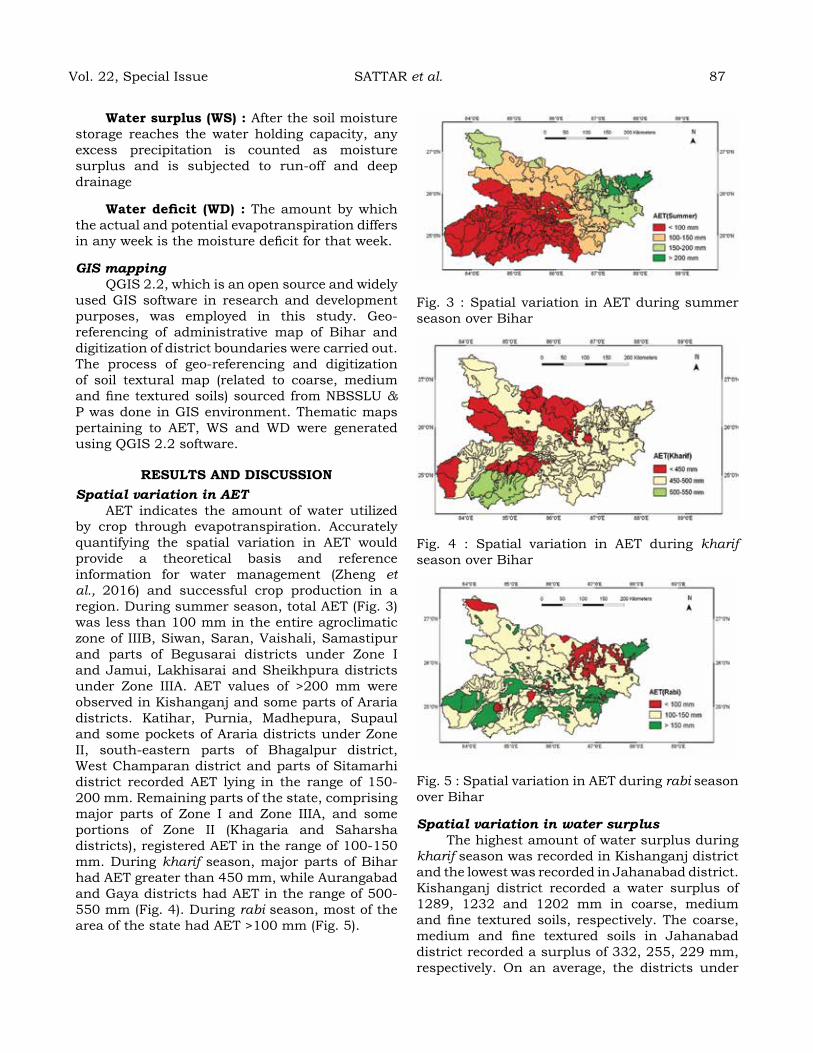
Water surplus (WS) : After the soil moisture storage reaches the water holding capacity, any excess precipitation is counted as moisture surplus and is subjected to run-off and deep drainage

Water deficit (Wd) : The amount by which the actual and potential evapotranspiration differs in any week is the moisture deficit for that week.

GIS mappingQGIS 2.2, which is an open source and widely

used GIS software in research and development purposes, was employed in this study. Geo-referencing of administrative map of Bihar and digitization of district boundaries were carried out. The process of geo-referencing and digitization of soil textural map (related to coarse, medium and fine textured soils) sourced from NBSSLU & P was done in GIS environment. Thematic maps pertaining to AET, WS and WD were generated using QGIS 2.2 software.

reSuLtS aNd dISCuSSIoNSpatial variation in AET

AET indicates the amount of water utilized by crop through evapotranspiration. Accurately quantifying the spatial variation in AET would provide a theoretical basis and reference information for water management (Zheng et al., 2016) and successful crop production in a region. During summer season, total AET (Fig. 3) was less than 100 mm in the entire agroclimatic zone of IIIB, Siwan, Saran, Vaishali, Samastipur and parts of Begusarai districts under Zone I and Jamui, Lakhisarai and Sheikhpura districts under Zone IIIA. AET values of >200 mm were observed in Kishanganj and some parts of Araria districts. Katihar, Purnia, Madhepura, Supaul and some pockets of Araria districts under Zone II, south-eastern parts of Bhagalpur district, West Champaran district and parts of Sitamarhi district recorded AET lying in the range of 150-200 mm. Remaining parts of the state, comprising major parts of Zone I and Zone IIIA, and some portions of Zone II (Khagaria and Saharsha districts), registered AET in the range of 100-150 mm. During kharif season, major parts of Bihar had AET greater than 450 mm, while Aurangabad and Gaya districts had AET in the range of 500-550 mm (Fig. 4). During rabi season, most of the area of the state had AET >100 mm (Fig. 5).

Fig. 3 : Spatial variation in AET during summer season over Bihar

Fig. 4 : Spatial variation in AET during kharif season over Bihar

Fig. 5 : Spatial variation in AET during rabi season over Bihar

Spatial variation in water surplusThe highest amount of water surplus during

kharif season was recorded in Kishanganj district and the lowest was recorded in Jahanabad district. Kishanganj district recorded a water surplus of 1289, 1232 and 1202 mm in coarse, medium and fine textured soils, respectively. The coarse, medium and fine textured soils in Jahanabad district recorded a surplus of 332, 255, 229 mm, respectively. On an average, the districts under

Vol. 22, Special Issue SATTAR et al. 87

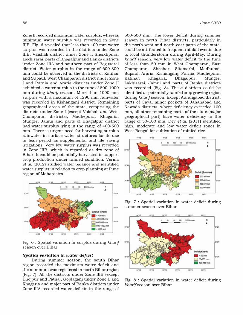
88 June 2020

Zone II recorded maximum water surplus, whereas minimum water surplus was recorded in Zone IIIB. Fig. 6 revealed that less than 400 mm water surplus was recorded in the districts under Zone IIIB, Vaishali district under Zone I, Sheikhpura, Lakhisarai, parts of Bhagalpur and Banka districts under Zone IIIA and southern part of Begusarai district. Water surplus in the range of 600-800 mm could be observed in the districts of Katihar and Supaul. West Champaran district under Zone I and Purnia and Araria districts under Zone II exhibited a water surplus to the tune of 800-1000 mm during kharif season. More than 1000 mm surplus with a maximum of 1290 mm rainwater was recorded in Kishanganj district. Remaining geographical areas of the state, comprising the districts under Zone I (except Vaishali and West Champaran districts), Madhepura, Khagaria, Munger, Jamui and parts of Bhagalpur district had water surplus lying in the range of 400-600 mm. There is urgent need for harvesting surplus rainwater in surface water structures for its use in lean period as supplemental and life saving irrigations. Very low water surplus was recorded in Zone IIIB, which is regarded as dry zone of Bihar. It could be potentially harvested to support crop production under rainfed condition. Verma et al. (2012) studied water balance and identified water surplus in relation to crop planning at Pune region of Maharastra.

Fig. 6 : Spatial variation in surplus during kharif season over Bihar

Spatial variation in water deficitDuring summer season, the south Bihar

region recorded the maximum water deficit and the minimum was registered in north Bihar region (Fig. 7). All the districts under Zone IIIB (except Bhojpur and Patna), Goplaganj under Zone I, and Khagaria and major part of Banka districts under Zone IIIA recorded water deficits in the range of

500-600 mm. The lower deficit during summer season in north Bihar districts, particularly in the north-west and north-east parts of the state, could be attributed to frequent rainfall events due to local thunderstorm during April-May. During kharif season, very low water deficit to the tune of less than 50 mm in West Champaran, East Champaran, Sheohar, Sitamarhi, Madhubai, Supaul, Araria, Kishanganj, Purnia, Madhepura, Katihar, Khagaria, Bhagalpur, Munger, Lakhisarai, Jamui and parts of Banka districts was recorded (Fig. 8). These districts could be identified as potentially rainfed crop growing region during kharif season. Except Aurangabad district, parts of Gaya, minor pockets of Jahanabad and Nawada districts, where deficiency exceeded 100 mm, all other remaining parts of the state (major geographical part) have water deficiency in the range of 50-100 mm. Dey et al. (2011) identified high, moderate and low water deficit zones in West Bengal for cultivation of rainfed rice.

Fig. 7 : Spatial variation in water deficit during summer season over Bihar

Fig. 8 : Spatial variation in water deficit during kharif season over Bihar

Water availability and crop prospectAppropriate crops could be fitted in the

cropping sequence in different crop growing seasons based on water availability in different districts of Bihar. The prospect of rainfed kharif crops in the entire northern strip of the state including south-east part appeared to be high owing to better water availability. These districts could be identified as potentially rainfed crop growing region during kharif season. Low water deficit during rabi season in the north-west part of the state could be used for successful growing of rainfed crops like chick pea, lentil and toria, particularly in the areas where there is adequate amount of moisture in the soil profile at the beginning of rabi season. Sattar and Khan (2016) assessed water availability in Samastipur district of Bihar for rainfed crop planning. The low water deficit of less than 200 mm in the north-west part of the state is attributed to winter rainfall from western disturbance. During summer season in north Bihar districts, particularly in the north-west and north-east parts of the state, there is high prospect of successful cultivation of crops like green gram, black gram, summer maize and vegetables.

CoNCLuSIoNSThematic maps comprising of AET, WS and

WD during kharif, rabi and summer seasons helped in assessing variation in water use and identifying high, moderate and low water deficit and surplus zones in different districts of Bihar. The information generated could be of immense use in agricultural water management and rain water harvesting. The study could serve as an important guideline in chalking out climate driven tactical and strategic crop planning for augmenting rainfed crop production in the state of Bihar.

reFereNCeSBapuji Rao, B., Rao, V.U.M., Sandeep, V.M.,

Shanthibhushan Chowdary, P. and Venkateswarlu, B. (2011) PET Calculator (V.3.0). All India Coordinated Research Project on Agrometeorology, Central Research Institute for Dryland Agriculture, Hyderabad-500059, A.P., India

Dey, S., Banerjee, Saon and Saha, A. (2011) Water

deficit patterns for cultivation of rainfed rice in the Lower Gangetic Plains of West Bengal. Jour Agril Physics. 11: 79-83.

NRAA. (2012) Prioritization of rainfed areas in India. Study Report 4, National Rainfed Area Authority (NRAA), Planning Commission, Govt. of India, New Delhi, pp.100

Rao, GGSN and Vyas, B.M. (1983) Risk analysis for kharif crop production under rainfed conditions in Nagaur district. Mausam. 34 (1) : 111-116.

Sattar, A. and Khan, S.A. (2016). Assessing climatic water balance and growing period length for crop planning under rainfed condition. Ind. J. Soil. Cons., 44 (1) :37-43.

Sattar, A., Khan, S.A., Banerjee, Saon and Nanda, M.K. (2019). Assessing sowing window and water availability of rainfed crops in eastern Indian state of Bihar for climate smart agricultural production. Theor Appl Climatol., 137:2321-2334 DOI 10.1007/s00704-018-2741-9.

Saxton K, E. and Rawls, W.J. (2006) Soil water characteristic estimates by texture and organic matter for hydrologic solutions. Soil Sci. Soc. Am. J., 70: 1569-1578.

Saxton, K.E. (2014) Personal communication.Thornthwaite, C.W. and Mather, J. R. (1955) The

water balance: Publication in Climatology, Drexel Institute of Technology, New Jersey, 8: 1-104.

Verma, I. J., Koppar, A. L., Balasubramanian, R., Jadhav, V. N., and Erande, R. S. (2012) Monthly climatic water balance at selected locations in India. Mausam. 63 (1) : 129-136.

Zheng, Han., Yu, Guirui., Wang, Qiufeng., Zhu, Xianjin., He, Honglin., Wang, Yanfen., Zhang, Junhui., Li, Yingnian., Zhao, Liang., Zhao, Fenghua., Shi, Peili., Wang, Huimin., Yan, Junhua., Zhang, Yiping. (2016). Spatial variation in annual actual evapotranspiration of terrestrial ecosystems in China: Results from eddy covariance measurements. Jour. of Geographical Sciences. 26 (10) : 1391-1411.

Vol. 22, Special Issue SATTAR et al. 89

Fruit drop pattern and phenological behavior under arid irrigated zone of Punjab in Kinnow mandarin (Citrus reticulata L.).

a K SaNgWaN, M K Batth, P K arora aNd SaNdeeP raheJaPunjab Agricultural University, Dr. J C Bakhshi Regional Research station, Abohar

Corresponding author: [email protected]

aBStraCtThe excessive fruit drop in this zone is a serious problem in Kinnow, which starts from blooming and continues till final harvesting. Keeping in view, the present investigation was carried out at experimental orchard of the Dr J C Bakhshi, RRS, Abohar, PAU. Flowering pattern was different during both the years and it starts somewhat early in 2017 i.e. on 15th of February whereas during 2018 bud initiation starts on 17th of February.Flower opening starts on 20th and 8th of March i.e. 35 and 20 days after appearance of flower bud in 2017 and 2018 respectively and reached to full bloom within 4 days in 2017. Whereas in 2018 eleven days were taken by the plants to come into full bloom. The maximum flower drop was observed on West and North side of the tree respectively during 2017 (81.7 and 80.2) and 2018 (84.1 and 83.5 %), while eastern and south side showed minimum flower drop during both the years i.e. (78.3 and 79.1) and (81.4 and 82.1 %). Fruit set percentage was also recorded maximum in East and North side (67.5 % and 61.2 %) of the tree. Maximum fruit drop was noticed in April (1493 and 1132) followed by May and minimum 9 and 11 fruit drop were observed in the month of December. Pre-mature and pre-harvest fruit drop was directly affected by average relative humidity and recorded maximum (44 and 36) in September.

Keywords: Kinnow; Fruit drop; Temperature; Humidity.

INtroduCtIoN

Citrus is very important perennial fruit crop of the world. The major growing regions are primarily confined between 40º north-south latitude. Citrus is grown in a wide agro–climatic conditions of India right from northern plain and central highlands. Different commercial cultivars viz. Darjeeling mandarin, Khasi mandarin are cultivated in north-east India, Nagpur mandarin in Central India. Coorg mandarin is cultivated in Coorg areas of South India, while Mosambi, Sathgudi in western part of Maharashtra and Andhra Pradesh. Kinnow mandarin is commercially grown in north-west India. India holds sixth position among the citrus growing countries. In India, Punjab is well known for the production of high quality citrus fruits. In Punjab Kinnowis most preferred cultivar due to its wider adaptability, high yield and more economic returns. Presently, Kinnow is being cultivated over an area of 51.6 thousand ha, with an annual production of 1208 thousand MT in the state. Despite of this significant growth in production and area, our productivity is far below to those of advanced countries.

The excessive pre mature fruit drop in this

zone is a serious problem in Kinnow, which starts from blooming and continues till final harvesting. Although efforts have been made to control the pre mature fruit drop by exogenous application of growth regulators, fungicides and nutritional management but no significant results were observed, emphasizing the importance of climatic conditions on the effectiveness of various treatments for fruit drop. Flowering in citrus is induced either through low temperature stress during winter or stress due to soil water deficit condition. Phenology refers to “the study of the timing of recurrent biological events, the causes of their timing with regard to biotic and a biotic forces and the interrelationship among phases of the same or different species” (Badeck et al., 2004). So there was a need to find out the general pattern of pre mature fruit drop in relation to weather conditions of the arid irrigated region of Punjab. Normally all citrus species produce huge flowering. The floral loads depend on different parameters, which includes cultivars, age of the plant and environmental conditions (Monselise, 1986). In subtropical regions, major blooming as well as vegetative sprouting in citrus fruits started during spring or when mean temperature increases. Usually less intense flushes are


observed during summer and fall months which produce almost entirely vegetative shoots. The fact that temperature played a major role in flower induction is well established and has been recognized by Valiente and Albrigo, 2004 and Nebauer et al., 2006. A number of authors also proposed that low temperature condition may be dual effect, first on releasing bud dormancy and second on flower induction (García-Luis et al., 1989 and Tisserat et al., 1990). Many species and varieties of citrus also showed a wide range of behaviors with regards to flowering time and response to the inductive conditions. Citrus flowering is a complex phenological process which is highly influenced by various interacting factors. In North India decrease in mean temperature considerably during winter resulted in to bud dormancy. The major bloom in all citrus species occurs during early spring (February-March) when temperature starts rising after cold winter and when soil moisture conditions are suitable (Hayes, 1970). In India March and April is found critical for citrus growth as the low temperature during nights remains favorable for growth, but high temperature exceeds beyond required limit which resulted into heavy drop of flowers and small fruit lets which ultimately leads to drastic reduction in fruit yield. Day time high temperature during floral differentiation shortens the development time and advances the date of anthesis. Regarding flower intensity, the longer exposer to low temperature increases floral induction, thus, increases the number of flowers per node, per sprouting and the tree (Poerwanto and Inoue, 1990). At higher temperature, citrus trees bloom sooner, fruits mature early, fruit size gets increased and acidity level of fruit juice remains low. The day and night temperature fluctuations result in better fruit colouring and sugar accumulation (Deris et al., 2003). Not much work has been done to study the growth pattern, fruiting and fruit drop pattern in Kinnow mandarin in semi-arid conditions of Punjab. Therefore, present investigation was conducted on nine years old plants of Kinnow mandarin grafted on Rough lemon rootstock having uniform size and age.

MaterIaLS aNd MethodSThe present investigation was carried out at

experimental orchard of the Dr J C Bakhshi, RRS, Abohar, PAU during cropping season of 2017-18 to 2018-19. The Abohar is located in the arid irrigated zone of Punjab in India and has typical semi-arid climate with cold winter and hot and dry

summers, where, the mean monthly temperature shows wide fluctuations during both winter and summer months. Total sixteen plants of Kinnow mandarin in four replication and four plants per replication having uniform size and vigor were taken for investigation. The recommended standard package of cultural practices for Kinnow mandarin was followed uniformly throughout the period. The date of bud initiation was recorded visually by regularly inspecting the plants and the time of bud first appeared on the shoot was tagged accordingly. Time of bud break for the developing buds was also note down on tha tday on which the green tips exhibited and first leaf tissue appeared. It was the stage of first morphological difference between vegetative and reproductive phase of the plant. The period between bud initiation to bud break was counted as numbers of days for bud break. Flower initiation date was recorded when 5 percent flower open and full bloom date was considered when more than 75 percent flowers open. The end of flowering was considered as the date at which only 5 percent flower remains open. Flowering duration was the time difference between start to end of flowering. Numbers of flower drop was the total numbers of flower/fruit let dropped per plant during flowering to fruiting period. Accordingly, different meteorological parameters data of both years were recorded from the Delta-T (WS-GP1) automatic weather station Observatory, situated at the station and the accumulated heat units required for attaining different stages were worked out as per the following formula used by Mendel (1969).

GDD/HU (ºCd) =aΣb (T.max + T.min) / 2 - 12.5

Where, GDD or HU = Growing Degree Days or Heat Units

T.max = maximum temperature

T.min = minimum temperature

a and b = starting to end date of a phenophase

Base temperature = 12.5°C for citrus species

After full bloom, fruit set in each cultivar was recorded and the percentage of fruit set was worked out on the basis of number of buds tagged and number of fruits that had set (Sharma et al., 2016)

Fruit set (%) =Total number of fruits set

× 100Number of flowers tagged

Vol. 22, Special Issue SANGWAN et al. 91

92 June 2020

Fruit drop data was collected twice in a week on every Monday and Friday and the number counted individually than total number of fruit drop was also calculated by adding them and average was calculated. Total weight of fruit drop was recorded by using weighing balance at the same time. Diameter of was calculated by using digital vernier caliper (Mitutoyo). Pathological fruit drop was counted separately by visual observation and physiological fruit drop was calculated by subtracting pathological fruit drop from total fruit drop. Correlation of phenological parameters was established with meteorological data and data was compared by using mean values and paired t-test.

reSuLtS aNd dISCuSSIoNFlowering

Flowering data was recorded in Kinnow mandarin during flowering period in 2017 and 2018. The reproductive stage started at the time of bud formation. Flower buds starts to appear somewhat early in 2017 i.e.on 15th of February where as during 2018 bud initiation starts on 17th of February. It may be due to low temperature in February 2018 as compared to 2017 which resulted in to delayed bud initiation. This is because of low temperature which causes buds inactive and higher temperature releases the stress which ultimately triggers the commencement of reproductive growth. Even the rate of flower bud development is also a temperature dependent phenomenon. As per Mendel (1969) the citrus can tolerate minimum of 12.5 to 13.0ºC and maximum of (limiting growth) 37.0-39.0ºC however the optimum temperature range is 23.0 to 34.0ºC.A similar trend was also observed by Sharma et al., (2016) in the different citrus cultivars at Hisar. A perusal of data given in Table-1 also revealed that number of days taken for bud break might be in relation with accumulated heat units.

Comparatively in 2017 the time span for transition from bud initiation to bud beak was seven days, which was numerically less during 2018 (9 days) and accumulated heat units of 46.12 and 45.5 ºC days, respectively. This is because of accumulated heat units that required by Kinnow mandarin for bud break. Similar type of finding reported by Sharma et al., (2016).

Initiation of flower opening starts on 20th and 8th of March i.e. 35 and 20 days after initiation of flower bud in 2017 and 2018, respectively. This clearly shows the role of temperature for attaining of particular stage. The flowering reached to full bloom within 4 days in 2017 due to sudden rise thereafter. Whereas in 2018 eleven days were taken by the plants to come into full bloom, due top revalence of low average as well as minimum temperature throughout the month as compared to the year 2017. Flowering completes on 29th and 27th of March during 2017 and 2018, respectively. Flowering duration was found of about 9 to 19 days in both years of study. The decrease in flower duration (table 1) during 2017 was mainly due to prevalence of low temperature during the first fortnight of March and sudden rise thereafter. Whereas, in March 2018 temperature is 3 to 4ºC higher as compare to 2017 from starting of March but remains constant and optimum throughout the period i.e. (Minimum temperature range from 12 to 16 ºC and average temperature in the range of 18 to 22ºC) enhance the duration. These results were in harmony with Lovatt et al., (1984) who reported that rate of flower development was positively correlated with growing degree days. Poerwanto and Inoue (1990) observed that the flower sprouting was also affected by diurnal temperature variations and found that flower sprouts within seven days at 30/30ºC, 11 days at 30/15ºC, 21 days at 15/30ºC, and 33 days at 15/15ºC, in Satsuma mandarin (Citrus unshiu

Table 1: Flowering pattern and fruit yield in Kinnow mandarin during 2017 and 2018.

ob-serva-tions /Year

time of Bud initia-tion

time of Bud Break

Bud Break Period (days)

Heat units accu-mulat-

ed

Initia-tion of Flower open-ing

Full Bloom

end of Flow-ering

Flow-ering dura-tion

(days)

total no of

Flowers dropped

total no of Fruits

total Yield

2017 15 Feb 21 Feb 7 46.1 20 March

24 March

29 March

9 9790 618.8 107.54

2018 17Feb 25 Feb 9 45.5 8 March

19 March

27 March

19 11635.67 843.2 136.76

CDat (0.05)

- - - - - -- - - - 2.77 3.18

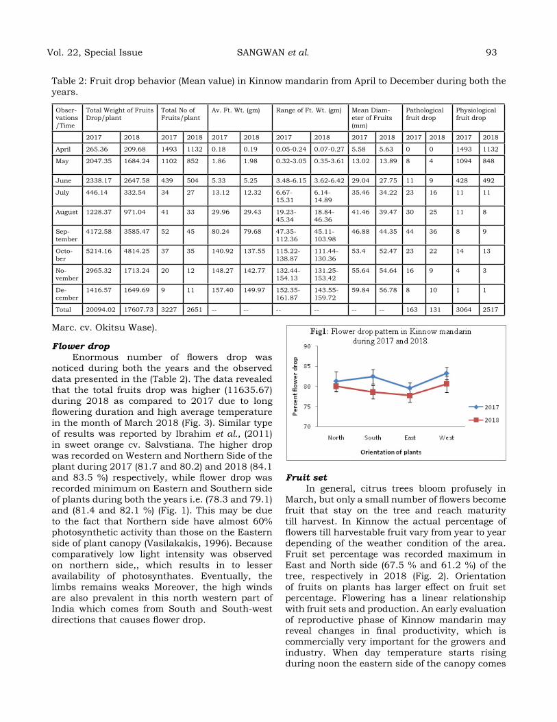
Marc. cv. Okitsu Wase).

Flower dropEnormous number of flowers drop was

noticed during both the years and the observed data presented in the (Table 2). The data revealed that the total fruits drop was higher (11635.67) during 2018 as compared to 2017 due to long flowering duration and high average temperature in the month of March 2018 (Fig. 3). Similar type of results was reported by Ibrahim et al., (2011) in sweet orange cv. Salvstiana. The higher drop was recorded on Western and Northern Side of the plant during 2017 (81.7 and 80.2) and 2018 (84.1 and 83.5 %) respectively, while flower drop was recorded minimum on Eastern and Southern side of plants during both the years i.e. (78.3 and 79.1) and (81.4 and 82.1 %) (Fig. 1). This may be due to the fact that Northern side have almost 60% photosynthetic activity than those on the Eastern side of plant canopy (Vasilakakis, 1996). Because comparatively low light intensity was observed on northern side,, which results in to lesser availability of photosynthates. Eventually, the limbs remains weaks Moreover, the high winds are also prevalent in this north western part of India which comes from South and South-west directions that causes flower drop.

Fruit setIn general, citrus trees bloom profusely in

March, but only a small number of flowers become fruit that stay on the tree and reach maturity till harvest. In Kinnow the actual percentage of flowers till harvestable fruit vary from year to year depending of the weather condition of the area. Fruit set percentage was recorded maximum in East and North side (67.5 % and 61.2 %) of the tree, respectively in 2018 (Fig. 2). Orientation of fruits on plants has larger effect on fruit set percentage. Flowering has a linear relationship with fruit sets and production. An early evaluation of reproductive phase of Kinnow mandarin may reveal changes in final productivity, which is commercially very important for the growers and industry. When day temperature starts rising during noon the eastern side of the canopy comes

Table 2: Fruit drop behavior (Mean value) in Kinnow mandarin from April to December during both the years.

Obser-vations /Time

Total Weight of Fruits Drop/plant

Total No of Fruits/plant

Av. Ft. Wt. (gm) Range of Ft. Wt. (gm) Mean Diam-eter of Fruits (mm)

Pathological fruit drop

Physiological fruit drop

2017 2018 2017 2018 2017 2018 2017 2018 2017 2018 2017 2018 2017 2018

April 265.36 209.68 1493 1132 0.18 0.19 0.05-0.24 0.07-0.27 5.58 5.63 0 0 1493 1132

May 2047.35 1684.24 1102 852 1.86 1.98 0.32-3.05 0.35-3.61 13.02 13.89 8 4 1094 848

June 2338.17 2647.58 439 504 5.33 5.25 3.48-6.15 3.62-6.42 29.04 27.75 11 9 428 492

July 446.14 332.54 34 27 13.12 12.32 6.67-15.31

6.14-14.89

35.46 34.22 23 16 11 11

August 1228.37 971.04 41 33 29.96 29.43 19.23-45.34

18.84-46.36

41.46 39.47 30 25 11 8

Sep-tember

4172.58 3585.47 52 45 80.24 79.68 47.35-112.36

45.11-103.98

46.88 44.35 44 36 8 9

Octo-ber

5214.16 4814.25 37 35 140.92 137.55 115.22-138.87

111.44-130.36

53.4 52.47 23 22 14 13

No-vember

2965.32 1713.24 20 12 148.27 142.77 132.44-154.13

131.25-153.42

55.64 54.64 16 9 4 3

De-cember

1416.57 1649.69 9 11 157.40 149.97 152.35-161.87

143.55-159.72

59.84 56.78 8 10 1 1

Total 20094.02 17607.73 3227 2651 -- -- -- -- -- -- 163 131 3064 2517


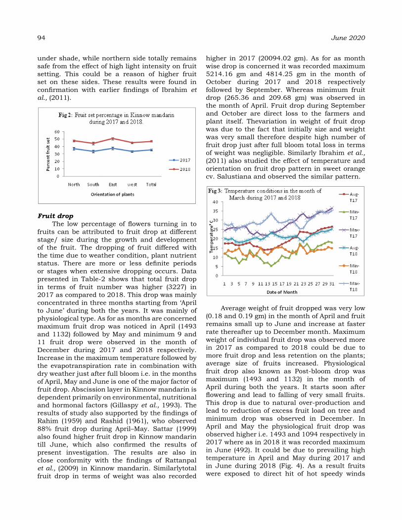
94 June 2020

under shade, while northern side totally remains safe from the effect of high light intensity on fruit setting. This could be a reason of higher fruit set on these sides. These results were found in confirmation with earlier findings of Ibrahim et al., (2011).

Fruit dropThe low percentage of flowers turning in to

fruits can be attributed to fruit drop at different stage/ size during the growth and development of the fruit. The dropping of fruit differed with the time due to weather condition, plant nutrient status. There are more or less definite periods or stages when extensive dropping occurs. Data presented in Table-2 shows that total fruit drop in terms of fruit number was higher (3227) in 2017 as compared to 2018. This drop was mainly concentrated in three months starting from ‘April to June’ during both the years. It was mainly of physiological type. As for as months are concerned maximum fruit drop was noticed in April (1493 and 1132) followed by May and minimum 9 and 11 fruit drop were observed in the month of December during 2017 and 2018 respectively. Increase in the maximum temperature followed by the evapotranspiration rate in combination with dry weather just after full bloom i.e. in the months of April, May and June is one of the major factor of fruit drop. Abscission layer in Kinnow mandarin is dependent primarily on environmental, nutritional and hormonal factors (Gillaspy et al., 1993). The results of study also supported by the findings of Rahim (1959) and Rashid (1961), who observed 88% fruit drop during April–May. Sattar (1999) also found higher fruit drop in Kinnow mandarin till June, which also confirmed the results of present investigation. The results are also in close conformity with the findings of Rattanpal et al., (2009) in Kinnow mandarin. Similarlytotal fruit drop in terms of weight was also recorded

higher in 2017 (20094.02 gm). As for as month wise drop is concerned it was recorded maximum 5214.16 gm and 4814.25 gm in the month of October during 2017 and 2018 respectively followed by September. Whereas minimum fruit drop (265.36 and 209.68 gm) was observed in the month of April. Fruit drop during September and October are direct loss to the farmers and plant itself. Thevariation in weight of fruit drop was due to the fact that initially size and weight was very small therefore despite high number of fruit drop just after full bloom total loss in terms of weight was negligible. Similarly Ibrahim et al., (2011) also studied the effect of temperature and orientation on fruit drop pattern in sweet orange cv. Salustiana and observed the similar pattern.

Average weight of fruit dropped was very low (0.18 and 0.19 gm) in the month of April and fruit remains small up to June and increase at faster rate thereafter up to December month. Maximum weight of individual fruit drop was observed more in 2017 as compared to 2018 could be due to more fruit drop and less retention on the plants; average size of fruits increased. Physiological fruit drop also known as Post-bloom drop was maximum (1493 and 1132) in the month of April during both the years. It starts soon after flowering and lead to falling of very small fruits. This drop is due to natural over-production and lead to reduction of excess fruit load on tree and minimum drop was observed in December. In April and May the physiological fruit drop was observed higher i.e. 1493 and 1094 respectively in 2017 where as in 2018 it was recorded maximum in June (492). It could be due to prevailing high temperature in April and May during 2017 and in June during 2018 (Fig. 4). As a result fruits were exposed to direct hit of hot speedy winds

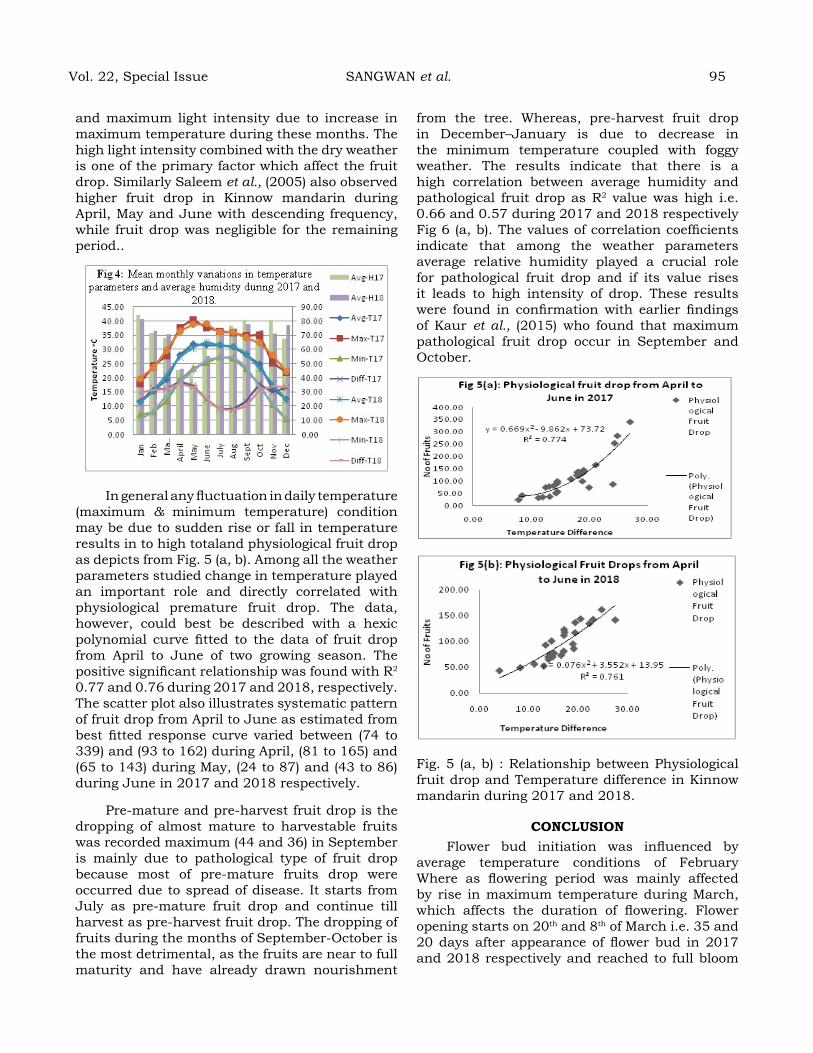
and maximum light intensity due to increase in maximum temperature during these months. The high light intensity combined with the dry weather is one of the primary factor which affect the fruit drop. Similarly Saleem et al., (2005) also observed higher fruit drop in Kinnow mandarin during April, May and June with descending frequency, while fruit drop was negligible for the remaining period..

In general any fluctuation in daily temperature (maximum & minimum temperature) condition may be due to sudden rise or fall in temperature results in to high totaland physiological fruit drop as depicts from Fig. 5 (a, b). Among all the weather parameters studied change in temperature played an important role and directly correlated with physiological premature fruit drop. The data, however, could best be described with a hexic polynomial curve fitted to the data of fruit drop from April to June of two growing season. The positive significant relationship was found with R2 0.77 and 0.76 during 2017 and 2018, respectively. The scatter plot also illustrates systematic pattern of fruit drop from April to June as estimated from best fitted response curve varied between (74 to 339) and (93 to 162) during April, (81 to 165) and (65 to 143) during May, (24 to 87) and (43 to 86) during June in 2017 and 2018 respectively.

Pre-mature and pre-harvest fruit drop is the dropping of almost mature to harvestable fruits was recorded maximum (44 and 36) in September is mainly due to pathological type of fruit drop because most of pre-mature fruits drop were occurred due to spread of disease. It starts from July as pre-mature fruit drop and continue till harvest as pre-harvest fruit drop. The dropping of fruits during the months of September-October is the most detrimental, as the fruits are near to full maturity and have already drawn nourishment

from the tree. Whereas, pre-harvest fruit drop in December–January is due to decrease in the minimum temperature coupled with foggy weather. The results indicate that there is a high correlation between average humidity and pathological fruit drop as R2 value was high i.e. 0.66 and 0.57 during 2017 and 2018 respectively Fig 6 (a, b). The values of correlation coefficients indicate that among the weather parameters average relative humidity played a crucial role for pathological fruit drop and if its value rises it leads to high intensity of drop. These results were found in confirmation with earlier findings of Kaur et al., (2015) who found that maximum pathological fruit drop occur in September and October.

Fig. 5 (a, b) : Relationship between Physiological fruit drop and Temperature difference in Kinnow mandarin during 2017 and 2018.

CoNCLuSIoNFlower bud initiation was influenced by

average temperature conditions of February Where as flowering period was mainly affected by rise in maximum temperature during March, which affects the duration of flowering. Flower opening starts on 20th and 8th of March i.e. 35 and 20 days after appearance of flower bud in 2017 and 2018 respectively and reached to full bloom


96 June 2020

within 4 and 11 days. The flower drop was high on West and South side of the tree during both the years due to less direct exposure to the radiations while minimum flower drop was observed on East and North side of plants. Fruit set percentage was also recorded maximum in East and North side (67.5 % and 61.2 %) of the tree. Maximum fruit drop was noticed in April (1493 and 1132) followed by May due to more fluctuation in temperature conditions. Pre-mature and pre-harvest fruit drop was directly affected by average relative humidity and recorded maximum (44 and 36) in September.

Fig. 6 (a, b) : Relationship between Pathological fruit drop and average humidity in Kinnow mandarin during 2017 and 2018.

reFereNCeS 1. Badeck, F., Bondeau, A., Böttcher, K.,

Doktor, D., Lucht, W. and Schaber, J. (2004). Responses of Spring Phenology to Climate Change. New Phytologist.162: 295-209.

2. Deris, R., Niskanen, R. and Jain, S. M. (2003). Crop Management and Postharvest Handling of Horticultural Products, Crop Fertilization, Nutrition and Growth. Science Publishers, USA. p. 284.

3. Garcia-Luis, A., Santamarina, P. and Guardiola, J.L. (1989). Flower formation from Citrus unshiu buds cultured in vitro. Ann. Bot. 64:515-519.

4. Gillaspy, G., David. H.B. and Gruissem, W. (1993). Fruits: a developmental perspective. J. Plant Cell. 5: 1439-1451.

5. Hayes, W. B. (1970). The citrus fruits. In: Fruit Growing in India, Kitabistan, Allahabad, India. pp. 196-266.

6. Ibrahim, M., Akhtar, N., Abbasi. Hafeez-ur-Rahman, Hussain, A. and Hafiz, I.A. (2011). Phenological behaviour and effect of different chemicals on pre-harvest fruit drop of sweet orange cv. ‘Salustiana’ .Pak. J. Bot 43 (1) : 453-457.

7. Kaur, S., Kanchan, B.B., Kumar, A. and Chahal, T.S. (2015). Prevalence of pre-harvest fruit drop disease of citrus in Punjab and in vitro evaluation of fungicides against pathogen. Pl. Dis.Res. J. 30 (1) :40-50.

8. Lovatt, C. J., Streeter, S. M., Minter, S. M., O’Connell, N. V., Flaherty, D. L., Freeman, M. W. and Goodell, P. B. (1984). Phenology of flowering in Citrus sinensis (L.) Osbeck, (Washington Navel orange) Proceedings of the International Society of Citriculture. 1:186-190.

9. Mendel, K. (1969). The influence of temperature and light on the vegetative development of citrus trees. Proceedings of the 1st International Citriculture Symposium, Citrus Congress, Riverside, California. 1: 259-265.

10. Monselise, S.P. (1986). Citrus. In: Monselise SP (ed), Handbook of Fruit Set and Development, CRC Press, Boca Raton. 87-108.

11. Nebauer, S.G., Avila, C., García-Luis, A. and Guardiola, J.L. (2006). Seasonal variation in the competence of the buds of three cultivars from different Citrus species to flower. Trees. 20:507-514.

12. Poerwanto, R. and Inoue, H. (1990). Effects of air and soil temperature on flower development and morphology of Satsuma mandarin. J. Horticultural Sciences. 65: 739-745.

13. Rahim, A. (1959). Some studies on the influence of rootstocks on the chemical composition, fruit maturity, grade and drop in Valencia orange. M.Sc. Thesis, University

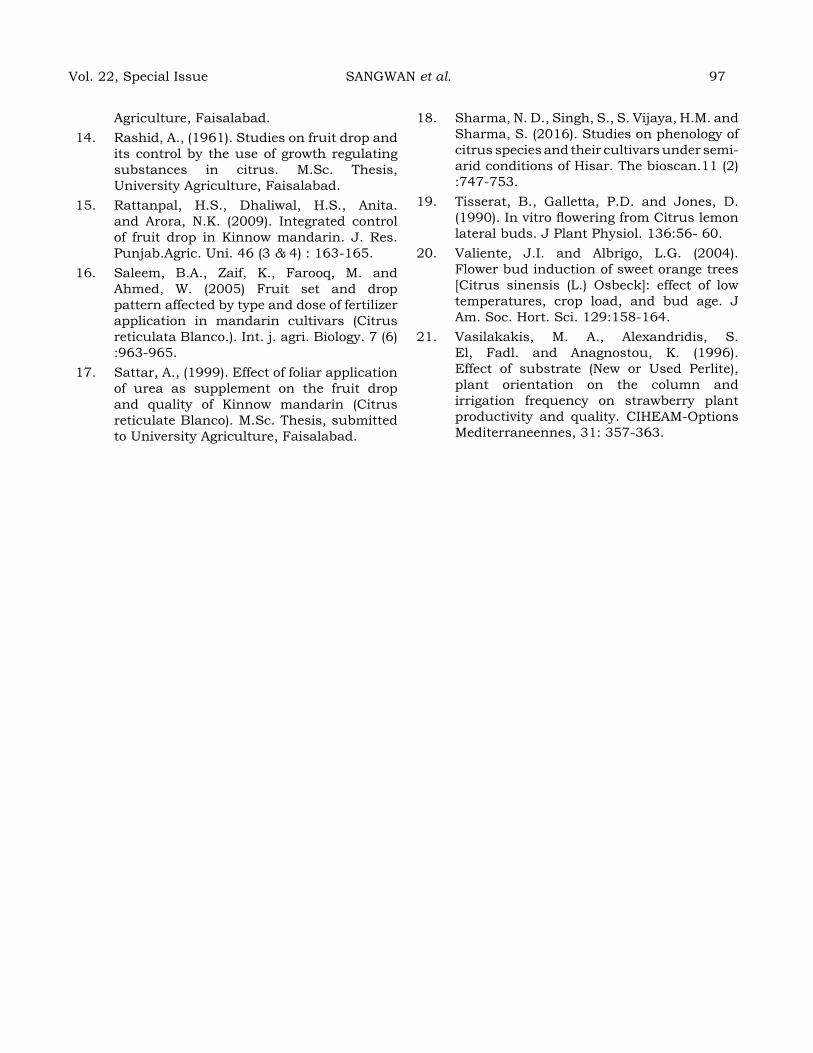
Agriculture, Faisalabad.14. Rashid, A., (1961). Studies on fruit drop and

its control by the use of growth regulating substances in citrus. M.Sc. Thesis, University Agriculture, Faisalabad.

15. Rattanpal, H.S., Dhaliwal, H.S., Anita.and Arora, N.K. (2009). Integrated control of fruit drop in Kinnow mandarin. J. Res. Punjab.Agric. Uni. 46 (3 & 4) : 163-165.

16. Saleem, B.A., Zaif, K., Farooq, M. and Ahmed, W. (2005) Fruit set and drop pattern affected by type and dose of fertilizer application in mandarin cultivars (Citrus reticulata Blanco.). Int. j. agri. Biology. 7 (6) :963-965.

17. Sattar, A., (1999). Effect of foliar application of urea as supplement on the fruit drop and quality of Kinnow mandarin (Citrus reticulate Blanco). M.Sc. Thesis, submitted to University Agriculture, Faisalabad.

18. Sharma, N. D., Singh, S., S. Vijaya, H.M. and Sharma, S. (2016). Studies on phenology of citrus species and their cultivars under semi-arid conditions of Hisar. The bioscan.11 (2) :747-753.

19. Tisserat, B., Galletta, P.D. and Jones, D. (1990). In vitro flowering from Citrus lemon lateral buds. J Plant Physiol. 136:56- 60.

20. Valiente, J.I. and Albrigo, L.G. (2004). Flower bud induction of sweet orange trees [Citrus sinensis (L.) Osbeck]: effect of low temperatures, crop load, and bud age. J Am. Soc. Hort. Sci. 129:158-164.

21. Vasilakakis, M. A., Alexandridis, S. El, Fadl. and Anagnostou, K. (1996). Effect of substrate (New or Used Perlite), plant orientation on the column and irrigation frequency on strawberry plant productivity and quality. CIHEAM-Options Mediterraneennes, 31: 357-363.


Sustaining rainfed maize productivity under varied eNSo events in tamil Nadu

veNgateSWarI M1*, geethaLaKShMI v2, BhuvaNeSWarI K3, PaNNeerSeLvaM S4

1Ph.D Scholar, Tamil Nadu Agricultural University, Coimbatore, 641 003, Tamil Nadu, India.2Director (DCM), Tamil Nadu Agricultural University, Coimbatore, 641 003, Tamil Nadu, India.

3Research Associate, M S Swaminathan Research Foundation, Chennai, 600 113, Tamil Nadu, India.4Director (WTC), Tamil Nadu Agricultural University, Coimbatore, 641 003, Tamil Nadu, India.


aBStraCtEl Niño Southern Oscillation (ENSO) is the dominant mode of climate variability on seasonal to inter-annual scales and its impacts are felt worldwide. ENSO often affects seasonal temperature, precipitation and thus crop yields in many regions especially in rainfed condition. In this present study, daily time series of weather data (1971-2013) at district scale obtained from India Meteorological Department and segregated under El Niño, La Niña and neutral years for the rainfed cropping period (RCP, September - December) to perform the analysis. CERES-Maize model embedded in DSSAT 4.6 was employed to simulate the maize productivity with ENSO episodes and adaptation option with different sowing windows. El Niño conditions positively influenced the rainfed cropping period rainfall. El Niño years recorded highest productivity (4203 kg ha-1) with less co-efficient of variation 13 per cent. In contrast the La Niña years recorded the lowest productivity (3423 kg ha-1) with 18 per cent of co-efficient of variation over Tamil Nadu. Yield gains for maize under El Niño, La Niña and Neutral for early sown (1 Sep) were 14.3, 8.6 and 13.0 % over the 15th September sowing and 18.0, 22.8 and 18.2 % over 1st October sowing.

INtroduCtIoN

Climate variability has been principal source of fluctuations in Indian food production and creating substantial challenges in crop production. Even though there is no long-term trend, inter-annual variability of Indian monsoon rainfall leading to frequent droughts and floods has profound influence on agriculture and in turn national economy (Rajeevan and Pai, 2006). Fluctuations of the climate are more relevant when considering crop production at an aggregate spatial scale. Since rainfall variations have direct impacts on the crop production, efforts need to be taken to utilize the El Niño Southern Oscillation (ENSO) - rainfall linkage for assessing the impact of ENSO on crop production and subsequent agricultural planning for the current climate. ENSO is the dominant mode of climate variability on seasonal to inter-annual scales and its impacts are felt worldwide (Trenberth, 1997). ENSO often affects seasonal temperature, precipitation and thus crop yields (Toshichi, 2014) in many regions especially in rainfed condition. Crop Productivity is highly dependent on climate and weather under rain-fed agriculture. Tamil Nadu has cultivated around 4.954 million ha of land which is 38 % of the total geographical area (Season and crop

report Tamil Nadu 2010-11, Directorate of Economics and Statistics, 2012), of which 42 % is rainfed and 58 % is irrigated (Department of Economics and Statistics, Tamil Nadu, 2010). Among all the major cereal crops cultivated under rainfed condition, maize is the most versatile emerging crop with greater adaptability under varying agro-climatic conditions. Globally, maize is known as “Queen” of cereals because it has the greatest potential for genetic yield among the cereals. Although there has been substantial growth in production, there is also substantial variability about the trend. Year to year weather variability is regarded as the primary cause of year to year fluctuations in yields. Adjusting the sowing window to match the critical crop growing period under favourable environment is one of the important adaptation strategies to manage the climate variability (Alam et al., 2007). Hence, it is important to find out the potential sowing window to offset the risks associated with climate variability during cropping season.

MaterIaLS aNd MethodSStudy area and data

Tamil Nadu is located in the Southernmost tip of the Indian Peninsula between 8°5’ and 13°35’ North latitude and 76°15’ and 80°20’


East longitude. Daily rainfall and temperature data at district scale was obtained from India Meteorological Department (IMD) for a period of 43 years from 1971 – 2013. Rainfall during El Niño, La Niña and neutral years was segregated for the rainfed cropping period (RCP, September - December) to perform the analysis.

Among the 32 districts of Tamil Nadu state, 30 districts such as Ariyalur, Coimbatore, Cuddalore, Dharmapuri, Dindigul, Erode, Kancheepuram, Kanniyakumari, Karur, Krishnakiri, Madurai, Nagapattinam, Namakkal, Perambalur, Pudukkottai, Ramanathapuram, Salem, Sivaganga, Thanjavur, Theni, Tiruchirappalli, Tirunelveli, Tiruppur, Thiruvallur, Tiruvannamalai, Thiruvarur, Thothukkudi, Vellore, Villupuram and Virudhunagar were considered for the study. The Nilgris district falls under hilly region and Chennai district were excluded from the study as it has no area on production of maize.

Table 1: El Niño, La Niña and neutral years from 1971 to 2013

el Niño La Niña Neutral1972, 1976, 1977, 19791982, 1986, 1987, 19911994, 1997, 2002, 20042006, 2009

1971, 1973, 1974, 19751983, 1984, 1988, 19951998, 1999, 2000, 20072010, 2011

1978, 1980, 1981, 19851989, 1990, 1992, 19931996, 2001, 2003, 20052008, 2012, 2013

Impact of ENSO on maize productivityIn the present study, CERES-Maize model

embedded in DSSAT 4.6 was employed to simulate the productivity of maize for 43 years and related with ENSO episodes.

Simulation of maize yield using DSSAT modelThe Decision Support System for Agro-

technology Transfer (DSSAT) is a micro-computer software product that combines crop, soil and weather data-bases into standard formats for access by crop models and application programs. The user can simulate multi-year outcomes of crop management strategies for different crops for any location in the world (Hoogenboom, 2000) and hence, the DSSAT was used in the present investigation.

(a) Weather fileThe daily weather data on maximum

temperature (°C), minimum temperature (°C) and rainfall (mm) for the period of 43 years (1971-2013) for the concerned district was collected from IMD. For crop simulation, solar radiation data is essential and it was generated using weather generator tool available in DSSAT crop simulation model using maximum and minimum temperatures as input.

(b) Soil data fileSoil information for creating the soil files was

obtained from the Department of Remote Sensing and Geographical Information System, TNAU. The profile details as required in DSSAT are extracted from the above remote sensing database using ArcGIS and were fed into S-Build tool in DSSAT to create soil file.

(c) Experimental detail fileExperimental file in DSSAT documents

the inputs including details of the experimental conditions and field characteristics such as weather station name, soil, and field description details, initial soil, water and inorganic nitrogen conditions, planting geometries, irrigation and water management, fertilizer management details, organic residue application, chemical applications, tillage operations, environmental modifications, harvest management and simulation controls (specification of simulation options e.g. starting dates, on/off options for water and nitrogen balances, symbiosis) and output options are given in the experimental file.

(d) Genetic co-efficient for maize Model calibration or parameterization is

the adjustment of genetic parameters so that simulated values compare well with observed values. Data obtained from the experiments were used to estimate genetic parameters. The genetic coefficients that influence the occurrence of developmental stages in the CERES - Maize coupled in DSSAT model were derived iteratively, by manipulating the relevant coefficients to achieve the best possible match between the simulated and observed number of days to the phenological events and grain yield at harvest. A detailed description of the cultivar coefficients used by CERES-Maize for TNAU maize hybrid CO6 is presented in Table 2.

Vol. 22, Special Issue VENGATESWARI et al. 99

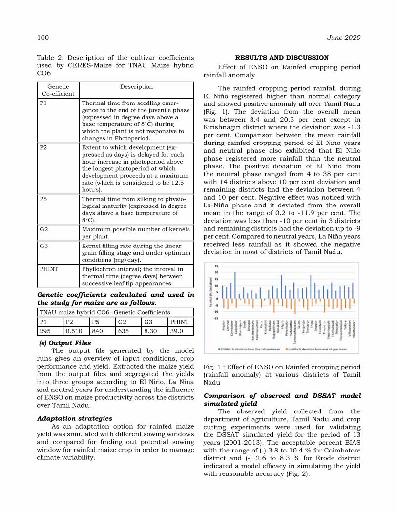
100 June 2020

Table 2: Description of the cultivar coefficients used by CERES-Maize for TNAU Maize hybrid CO6

Genetic Co-efficient

Description

P1 Thermal time from seedling emer-gence to the end of the juvenile phase (expressed in degree days above a base temperature of 8°C) during which the plant is not responsive to changes in Photoperiod.

P2 Extent to which development (ex-pressed as days) is delayed for each hour increase in photoperiod above the longest photoperiod at which development proceeds at a maximum rate (which is considered to be 12.5 hours).

P5 Thermal time from silking to physio-logical maturity (expressed in degree days above a base temperature of 8°C).

G2 Maximum possible number of kernels per plant.

G3 Kernel filling rate during the linear grain filling stage and under optimum conditions (mg/day).

PHINT Phyllochron interval; the interval in thermal time (degree days) between successive leaf tip appearances.

Genetic coefficients calculated and used in the study for maize are as follows.TNAU maize hybrid CO6- Genetic CoefficientsP1 P2 P5 G2 G3 PHINT295 0.510 840 635 8.30 39.0

(e) Output FilesThe output file generated by the model

runs gives an overview of input conditions, crop performance and yield. Extracted the maize yield from the output files and segregated the yields into three groups according to El Niño, La Niña and neutral years for understanding the influence of ENSO on maize productivity across the districts over Tamil Nadu.

Adaptation strategies As an adaptation option for rainfed maize

yield was simulated with different sowing windows and compared for finding out potential sowing window for rainfed maize crop in order to manage climate variability.

reSuLtS aNd dISCuSSIoNEffect of ENSO on Rainfed cropping period

rainfall anomaly

The rainfed cropping period rainfall during El Niño registered higher than normal category and showed positive anomaly all over Tamil Nadu (Fig. 1). The deviation from the overall mean was between 3.4 and 20.3 per cent except in Kirishnagiri district where the deviation was -1.3 per cent. Comparison between the mean rainfall during rainfed cropping period of El Niño years and neutral phase also exhibited that El Niño phase registered more rainfall than the neutral phase. The positive deviation of El Niño from the neutral phase ranged from 4 to 38 per cent with 14 districts above 10 per cent deviation and remaining districts had the deviation between 4 and 10 per cent. Negative effect was noticed with La-Niña phase and it deviated from the overall mean in the range of 0.2 to -11.9 per cent. The deviation was less than -10 per cent in 3 districts and remaining districts had the deviation up to -9 per cent. Compared to neutral years, La Niña years received less rainfall as it showed the negative deviation in most of districts of Tamil Nadu.

Fig. 1 : Effect of ENSO on Rainfed cropping period (rainfall anomaly) at various districts of Tamil Nadu

Comparison of observed and DSSAT model simulated yield

The observed yield collected from the department of agriculture, Tamil Nadu and crop cutting experiments were used for validating the DSSAT simulated yield for the period of 13 years (2001-2013). The acceptable percent BIAS with the range of (-) 3.8 to 10.4 % for Coimbatore district and (-) 2.6 to 8.3 % for Erode district indicated a model efficacy in simulating the yield with reasonable accuracy (Fig. 2).

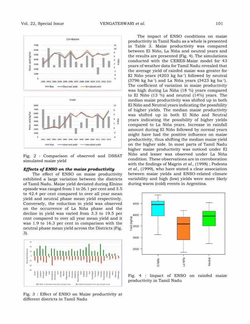
Fig. 2 : Comparison of observed and DSSAT simulated maize yield

Effects of ENSO on the maize productivity The effect of ENSO on maize productivity

exhibited a large variation between the districts of Tamil Nadu. Maize yield deviated during Elnino episode was ranged from 1 to 26.1 per cent and 3.5 to 42.4 per cent compared to over all year mean yield and neutral phase mean yield respectively. Conversely, the reduction in yield was observed on the occurrence of La Niña phase and the decline in yield was varied from 3.3 to 19.5 per cent compared to over all year mean yield and it was 1.9 to 16.3 per cent in comparison with the neutral phase mean yield across the Districts (Fig. 3).

Fig. 3 : Effect of ENSO on Maize productivity at different districts in Tamil Nadu

The impact of ENSO conditions on maize productivity in Tamil Nadu as a whole is presented in Table 3. Maize productivity was compared between El Niño, La Niña and neutral years and the results are presented (Fig. 4). The simulations conducted with the CERES-Maize model for 43 years of weather data for Tamil Nadu revealed that the average yield of rainfed maize was greater for El Niño years (4203 kg ha-1) followed by neutral (3796 kg ha-1) and La Niña years (3423 kg ha-1). The coefficient of variation in maize productivity was high during La Niña (18 %) years compared to El Niño (13 %) and neutral (14%) years. The median maize productivity was shifted up in both El Niño and Neutral years indicating the possibility of higher yields. The median maize productivity was shifted up in both El Niño and Neutral years indicating the possibility of higher yields compared to La Niña years. Increase in rainfall amount during El Niño followed by normal years might have had the positive influence on maize productivity, thus shifting the median maize yield on the higher side. In most parts of Tamil Nadu higher maize productivity was noticed under El Niño and lesser was observed under La Niña condition. These observations are in corroboration with the findings of Magrin et al., (1998) ; Podesta et al., (1999), who have stated a clear association between maize yields and ENSO-related climate variability and high (low) yields were more likely during warm (cold) events in Argentina.

Fig. 4 : Impact of ENSO on rainfed maize productivity in Tamil Nadu


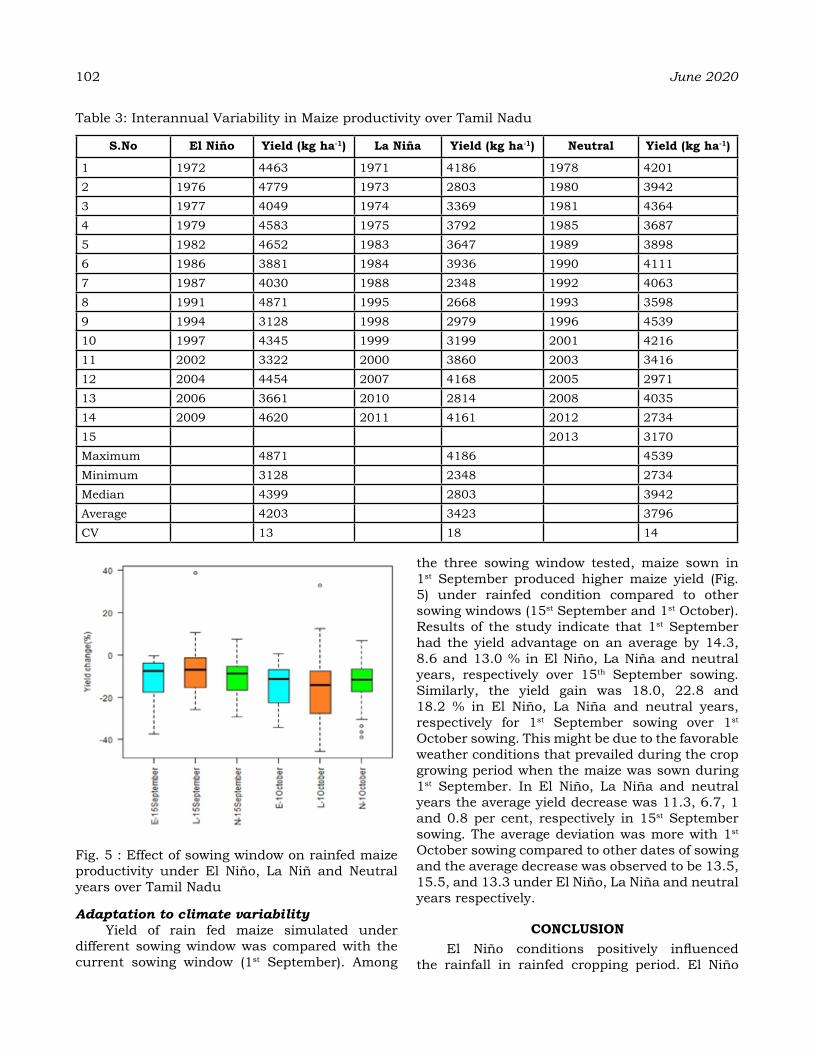
102 June 2020

Fig. 5 : Effect of sowing window on rainfed maize productivity under El Niño, La Niñ and Neutral years over Tamil Nadu

Adaptation to climate variability Yield of rain fed maize simulated under

different sowing window was compared with the current sowing window (1st September). Among

the three sowing window tested, maize sown in 1st September produced higher maize yield (Fig. 5) under rainfed condition compared to other sowing windows (15st September and 1st October). Results of the study indicate that 1st September had the yield advantage on an average by 14.3, 8.6 and 13.0 % in El Niño, La Niña and neutral years, respectively over 15th September sowing. Similarly, the yield gain was 18.0, 22.8 and 18.2 % in El Niño, La Niña and neutral years, respectively for 1st September sowing over 1st October sowing. This might be due to the favorable weather conditions that prevailed during the crop growing period when the maize was sown during 1st September. In El Niño, La Niña and neutral years the average yield decrease was 11.3, 6.7, 1 and 0.8 per cent, respectively in 15st September sowing. The average deviation was more with 1st October sowing compared to other dates of sowing and the average decrease was observed to be 13.5, 15.5, and 13.3 under El Niño, La Niña and neutral years respectively.

CoNCLuSIoNEl Niño conditions positively influenced

the rainfall in rainfed cropping period. El Niño

Table 3: Interannual Variability in Maize productivity over Tamil Nadu

S.No el Niño Yield (kg ha-1) La Niña Yield (kg ha-1) Neutral Yield (kg ha-1)

1 1972 4463 1971 4186 1978 42012 1976 4779 1973 2803 1980 39423 1977 4049 1974 3369 1981 43644 1979 4583 1975 3792 1985 36875 1982 4652 1983 3647 1989 38986 1986 3881 1984 3936 1990 41117 1987 4030 1988 2348 1992 40638 1991 4871 1995 2668 1993 35989 1994 3128 1998 2979 1996 453910 1997 4345 1999 3199 2001 421611 2002 3322 2000 3860 2003 341612 2004 4454 2007 4168 2005 297113 2006 3661 2010 2814 2008 403514 2009 4620 2011 4161 2012 273415 2013 3170Maximum 4871 4186 4539Minimum 3128 2348 2734Median 4399 2803 3942Average 4203 3423 3796CV 13 18 14

years recorded highest productivity (4203 kg ha-1) with less CV (13 %). In contrast the La Niña years recorded the lowest productivity (3423 kg ha-1) with 18 per cent of co-efficient of variation over Tamil Nadu. The median maize productivity was shifted up in both El Niño and Neutral years indicating the possibility of higher yields compared to La Niña years. The performance of 1st September sowing was found to be better under El Niño, La Niña as well as neutral conditions in most parts of Tamil Nadu.

reFereNCeSAlam, M., A. Rahman, M. Rashid, G. Rabbani,

P. Bhandary, S. Bhadwal, M. Lal and M. H. Soejachmoen. 2007. Impacts, Vulnerability and Adaptation to Climate Change in Asia: Background Paper for Meeting on Adaptation, Beijing, China, 11-13 April. 2007. United Nations Framework Convention on Climate Change (UNFCCC).

Department of Economics and Statistics. 2010. Annual report, Department of Economics and Statistics, Tamil Nadu State, Chennai. http://www.tnstat.gov.in/ annualeport2010.pdf

Directorate of Economics and Statistics. 2012.Second Advanced Estimates of Production of Foodgrains for 2011-12, Agricultural Statistics Division, Directorate of Economics & Statistics, Department of Agriculture & Cooperation, Ministry of Agriculture, Govt. of India, New Delhi. http://agricoop.nic.in/sia111213312.pdf

Hoogenboom, G. 2000. Contribution of agrometeorology to the simulation of crop production and its applications. Agric. For.Meteorol. 103 (1–2) :137–157.

Magrin, G.O., M. O. Grondona, M. I. Travasso, D. R. Boullón, G. R. Rodriguez and C. Messina. 1998. Impacto del fenomeno “El Niño” sobre la produccion de cultivos en la region pampeana (Impact of the “El Niño” phenomenon on crop production in the Pampas). Instituto Nacional de Tecnologıa Agropecuaria (INTA), Instituto de Clima y Agua, 16 pp. Available from INTA, Castelar 1712, Buenos Aires, Argentina.

Podesta, G.P., C. D. Messina, M. O. Grondona and G. O. Magrin.1999. Associations between grain crop yields in central-eastern Argentina and El Niño-southern oscillation.J. Appl. Meteorol., 38: 1488–1498.

Rajeevan, M. and D.S. Pai. 2006. El-Nino Indian monsoon predictive relationships. National Climate Centre Research Report No http://www.imdpune.gov.in/ ncc_rept/RESEARCH%20REPORT%204.pdf

Toshichi, K., J. J. Luo, A. Challinor, G. Sakurai, M. Yokozawa, H. Sakuma, M. E. Brown and T. Yamagata. 2014. Impacts of El Niño Southern Oscillation on the global yields of major crops. Nature.DOI: 10.1038/ncomms4712

Trenberth, K. 1997. Short-term climate variations: recent accomplishments and issues for future progress. Bull. Am. Meteorol. Soc., 78: 1081–1096.


assessing yield-weather relationships in kharif maize under Punjab conditions using data mining method

BaruN BISWaS* aNd JagdISh SINghPAU Regional Research Station, Gurdaspur – 143521Punjab Agricultural University, Ludhiana – 141 004

*Email: [email protected]

aBStraCtThis study explored applicability of data mining technique Random Forest (RF) to access kharif maize yield and its relationship with different climatic variables under central and north Punjab conditions. The climatic variables were decomposed into 27 variables to capture their influence on different growth stages of maize totaling to final crop yield. One RF model was designed for each region to capture influence of different climatic predictors on kharif maize yield on regional scale. The average yield variation explained by climatic variables using an ensemble of 100 runs for each model was 21 percent for central Punjab and 28 percent for north Punjab. The variance influence scores showed that most influential variable was maximum temperature during reproductive phase over central Punjab region and rainfall during vegetative phase over north Punjab region. The partial dependence plots were prepared to explore exact roles of individual variables in explaining maize yield.

Keywords: Maize, yield-weather relation, data mining, random forest, variable importance.

INtroduCtIoN

The climate change and climatic variability in recent past have emerged as major obstacle for the achievement of world food production goals. As a result, sustainable agricultural practices, mitigating adverse effects of the changing climatic scenario, have become popular to meet increasing demand. Maize (Zea mays L.) is one of the most genetically versatile crops having wider adaptability under diverse agro-climatic conditions. In India, maize occupied 86.27 lakh ha area and production was about 210.2 lakh tones In Punjab, it covers 116 thousand hectares with total production of 445 thousand tonnes during 2016-2017. The average yield was 38.35 quintal per hectare (Anonymous, 2018). Therefore, cultivation of maize with proper management practices and farm planning may provide an alternative to widely adopted rice-wheat crop rotation in Punjab.

The growth and development of maize is affected by weather and climatic factors in many ways from sowing to till harvesting. Tao et al., (2003) described that changes in temporal and spatial pattern of precipitation in the growing season may directly impact the crop water cycle and could induce water stress during crop development. They also inferred that change in temperature from optimum ranges may increase the evapotranspiration and induce drought stress

in maize crop.

Due to complex relations between crop growth and environmental factors, identification of major yield governing factors often becomes critical task. Big observational crop yield and weather database available at regional level are often infected with large noise, non-linearity and high intervariable correlations. Statistical modelling methods based on data mining algorithms can provide alternatives to traditional regression approaches and overcome some of their limitations. (Jeong et al., 2016).

The data mining vis-à-vis machine learning techniques are becoming popular tool in recent times incrop yield and weather relation studies (Oguntunde et al., 2018). Among data mining techniques, random forest (RF) model is very popular for handling large number of causal variables and use “bagging” technique to identify most appropriate variable related to the dependent variable under consideration (Breiman, 2001) in comparison to widely used regression techniques. In this study, the major objective was to explore the data mining technique ‘random forest’ to identify major weather factors which contribute most tofinal yield of kharif maize yield in Punjab.


Major kharif maize producing districts


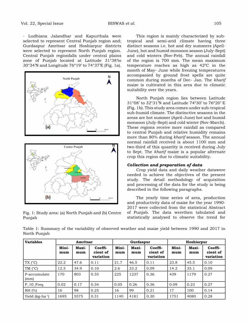
- Ludhiana Jalandhar and Kapurthala were selected to represent Central Punjab region and; Gurdaspur Amritsar and Hoshiarpur districts were selected to represent North Punjab region. Central Punjab regionfalls under central plains zone of Punjab located at Latitude 31°38’to 30°34’N and Longitude 76º19’ to 74°37’E (Fig. 1a).

Fig. 1: Study area: (a) North Punjab and (b) Centre Punjab

This region is mainly characterized by sub-tropical and semi-arid climate having three distinct seasons i.e. hot and dry summers (April-June), hot and humid monsoon season (July-Sept) and cold winters (Nov-Feb). The annual rainfall of the region is 700 mm. The mean maximum temperature reaches as high as 420C in the month of May- June while freezing temperatures accompanied by ground frost spells are quite common during months of Dec- Jan. The kharif maize is cultivated in this area due to climatic suitability over the years.

North Punjab region lies between Latitude 31°08’ to 32°31’N and Latitude 74030’ to 76º20’ E (Fig. 1b). This study area comes under sub-tropical sub-humid climate. The distinctive seasons in the areas are hot summer (April-June) hot and humid monsoon (July-Sept) and cold winter (Nov-March). These regions receive more rainfall as compared to central Punjab and relative humidity remains more than 80% during kharif season. The annual normal rainfall received is about 1100 mm and two-third of this quantity is received during July to Sept. The kharif maize is a popular alternate crop this region due to climatic suitability.

Collection and preparation of dataCrop yield data and daily weather datawere

needed to achieve the objectives of the present study. The detail methodology of acquisition and processing of the data for the study is being described in the following paragraphs.

The yearly time series of area, production and productivity data of maize for the year 1990-2017 were collected from the statistical Abstract of Punjab. The data werethen tabulated and statistically analysed to observe the trend for

Table 1: Summary of the variability of observed weather and maize yield between 1990 and 2017 in North Punjab

variables amritsar gurdaspur hoshiarpurMini-mum

Maxi-mum

Coeffi-cient of

variation

Mini-mum

Maxi-mum

Coeffi-cient of

variation

Mini-mum

Maxi-mum

Coeffi-cient of

variationTX (°C) 22.2 47.6 0.11 21.7 46.5 0.11 23.8 45.5 0.10TM (°C) 12.5 34.9 0.10 2.6 33.2 0.09 14.2 35.1 0.09P-accumulate (mm)

170 803 0.35 225 1237 0.36 439 1179 0.27

P_10_Freq 0.02 0.17 0.34 0.05 0.26 0.36 0.09 0.23 0.27RH (%) 16 98 0.25 16 99 0.21 17 100 0.14Yield (kg-ha-1) 1695 5575 0.31 1140 4181 0.30 1751 4080 0.28

Vol. 22, Special Issue BISWAS et al. 105

106 June 2020

further use in development of random forest models.

The daily weather record for the districts mentioned above was collected from surface observations and automatic weather station installed at each district. The data wereprovided by the Department of Climate Change and Agricultural Meteorology, PAU Ludhiana, PAU Regional Research Station, Gurdaspur and Meteorological Centre, IMD, Chandigarh. The complete series of 27 years (1990-2017) data were available only for Ludhiana. The missing data for rest of the district was generated by method described below. The five most important weather parameters for maize growth were considered: maximum temperature (tx), minimum temperature (tn), precipitation (rn), morning and evening relative humidity (rh). The summary of the variability present in both the maize growing regions are presented in Table 1 and 2.

Missing weather data generationThe missing weather data for different

districts were filled with high resolution grid data downloaded from NOAA data portal (Anonymous, 2018). But the relative humidity data was not available in the gridded data set. So, RH data was generated using popular weather generator MT-CLIM (Hungerford et al., 1989).

Preparation of dataThe weather data was further processed

following Cock et al., (2011) and Delerce et al., (2016). The present study was focused on maize yield being affected by weather factors. Individual yield data were related to daily weather data for different cropping events between sowing and

harvesting. The five metrological factors selected earlier were used to delineate the cropping events during maize growth period. The raw weather data were separated by diving maize growing period into three stages - vegetative (V) from germination to initiation of tasseling and cob, reproductive (R) from cob development to end of silking/pollination and grain filling (G) from kernel development to physiological maturity. The length of each growing period was calculated according to the major cultivars grown in the respective study areas. The resulting variables are listed in Table 3 where each weather element appears three times, one foreach growth stage.

Data mining technique to detect major climatic factors affecting maize yield

Data mining vis-à-vis machine learning techniques have become well accepted in several disciplines (Cutler et al., 2007; Das et al., 2009) to analyse large observational data as they have nonlinear or random relation among variables. Researchers have already used several data mining algorithms in earlier studies (Drummond et al., 2003; Cutler et al., 2007; Pons et al., 2009; Delmotte et al., 2011) to establish crop weather relationship. The main characteristics of the present problem was (i) noisy data in both predictor variables and response variable, (ii) non linear relationship between climatic variables and maize yield, (iii) multicollinearity exists among predictors and (iv) the need to retrieve relevant climatic variables which actually explain the kharif maize yield variability in Punjab. Based on available literatures, several algorithms were compared before identifying most suitable for the present study. This study did not compare

Table 2: Summary of the variability of observedweather and maize yield between 1990 and 2017 in North Punjab

variable Ludhiana Jalandhar KapurthalaMini-mum

Maxi-mum

Coeffi-cient of

variation

Mini-mum

Maxi-mum

Coeffi-cient of

variation

Mini-mum

Maxi-mum

Coefficient of variation

TX (°C) 22.6 46.6 0.10 23.6 47.1 0.10 22.8 47.5 0.10TM (°C) 0 126.9 0.12 14.1 33.6 0.09 13.3 34.3 0.09P-accumu-late (mm)

317 1087 0.34 305 984 0.29 194 819 0.33

P_10_Freq 0.06 0.19 0.24 0.05 0.19 0.30 0.02 0.16 0.34RH (%) 17 100 0.22 17 97 0.25 17 97 0.25Yield (kg-ha-1)

1754 4407 0.26 1913 5552 0.26 1545 6616 0.38

the algorithms in terms of prediction power since the main objective of the study was to explain variability and identify influential variables rather than to predict respond variable correctly. Shmaueli (2010) was followed to explain the variability in kharif maize yield in relation to climatic parameters.

Considering data nature, tree-based algorithm, i.e., random forest (Breiman, 2001) was

selected to achieve the goals of the study. Recently random forest (RF) have become a popular and widely used non-parametric regression tool in many scientific areas. This algorithm can explain high variability and are applicable in high dimensional with highly correlated variables (Strobl et al., 2008). Recently, the variable importance (VI) measured by RF have been used for identifying in relevant predictable variables,

Table 3: Lists of variables used in model development

variable name Meaning type unit

Cultivar Cultivar that was grown Categoricaltx_V Average maximum temperature in vegetative stage Continuous °Ctx_R Average maximum temperature in reproductive stage Continuous °Ctx_G Average maximum temperature in grain development stage Continuous °Ctn_V Average minimum temperature in vegetative stage Continuous °Ctn_R Average minimum temperature in reproductive stage Continuous °Ctn_G Average minimum temperature in grain development stage Continuous °Cta_V Average temperature in vegetative stage Continuous °Cta_R Average temperature in reproductive stage Continuous °Cta_G Average temperature in grain development stage Continuous °Ctd_V Average diurnal range in vegetative stage Continuous °Ctd_R Average diurnal range in reproductive stage Continuous °Ctd_G Average diurnal range in grain development stage Continuous °Ct40 frequency of days with maximum temperature above 40°C in

vegetative stageContinuous —

t37 frequency of days with maximum temperature above 37°C in reproductive stage

Continuous —

t34 frequency of days with maximum temperature above 34°C in grain development stage

Continuous —

rn_V Accumulated precipitation in vegetative stage Continuous mmrn_R Accumulated precipitation in reproductive stage Continuous mmrn_G Accumulated precipitation in grain development stage Continuous mmrf_10V Frequency of days with more than 10 mm precipitation in vege-

tative stageContinuous —

rf_10R Frequency of days with more than 10 mm precipitation in repro-ductive stage

Continuous —

rf_10G Frequency of days with more than 10 mm precipitation in grain development stage

Continuous —

rh_V Average relative humidity in vegetative stage Continuous %rh_R Average relative humidity in reproductive stage Continuous %rh_G Average relative humidity in grain development stage Continuous %rday_V Accumulated rainy days in vegetative stage Continuous -rday_R Accumulated rainy days in reproductive stage Continuous -rday_G Accumulated rainy days in grain development stage Continuous -Yield Crop productivity Continuous Kg-ha-1


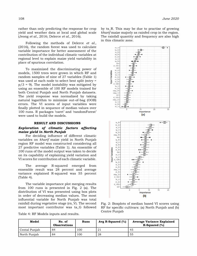
108 June 2020

rather than only predicting the response for crop yield and weather data at local and global scale (Jeong et al., 2016; Delerce et al., 2016).

Following the methods of Delerce et al., (2016), the random forest was used to calculate variable importance for better assessment of the contribution of the individual climatic variables at regional level to explain maize yield variability in place of spurious correlation.

To maximized the discriminating power of models, 1500 trees were grown in which RF and random samples of nine of 27 variables (Table 1) was used at each node to select best split (mtry = p/3 = 9). The model instability was mitigated by using an ensemble of 100 RF models trained for both Central Punjab and North Punjab datasets. The yield response was normalized by taking natural logarithm to minimize out-of-bag (OOB) errors. The VI scores of input variables were finally plotted in sequence of median values over 100 runs. R packages ‘caret’ and ‘randomForest’ were used to build the models.

reSuLt aNd dISCuSSIoNSExploration of climatic factors affecting maize yield in North Punjab

For deciding influence of different climatic variables on kharif maize yield in North Punjab region RF model was constructed considering all 27 predictive variables (Table 1). An ensemble of 100 runs of the model output was taken to decide on its capability of explaining yield variation and VI scores for contribution of each climatic variable.

The average R-squared emerged from ensemble result was 28 percent and average variance explained R-squared was 55 percent (Table 4).

The variable importance plot merging results from 100 runs is presented in Fig. 2 (a). The distribution of VI was presented using box plots in order of decreasing median values. The most influential variable for North Punjab was total rainfall during vegetative stage (rn_V). The second most important contributor was ta_G followed

by tx_R. This may be due to practise of growing kharif maize majorly as rainfed crop in the region. The rainfall quantity and frequency are also high in this climatic zone.

Fig. 2: Boxplots of median based VI scores using RF for specific cultivars: (a) North Punjab and (b) Centre Punjab

Table 4: RF Models inputs and results.

Model No. of observations

runs avg r-Squared (%) average variance explained r-Squared (%)

Cental Punjab 84 100 21 45North Punjab 84 100 28 55

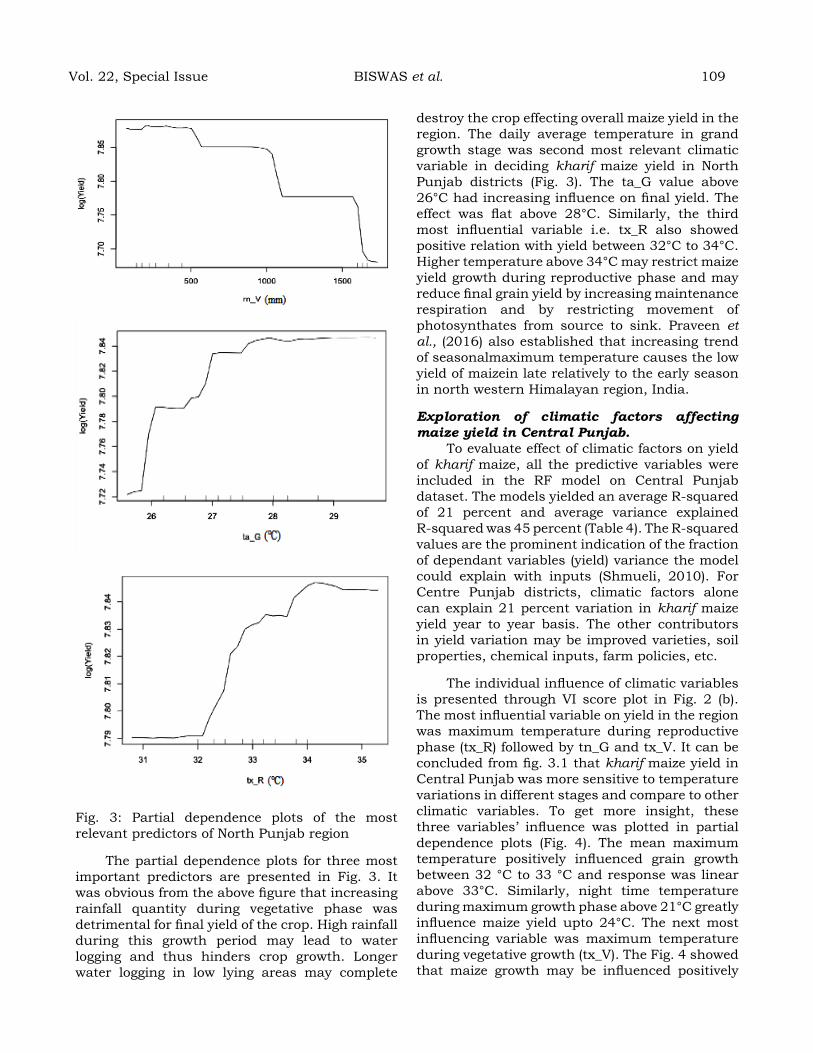
Fig. 3: Partial dependence plots of the most relevant predictors of North Punjab region

The partial dependence plots for three most important predictors are presented in Fig. 3. It was obvious from the above figure that increasing rainfall quantity during vegetative phase was detrimental for final yield of the crop. High rainfall during this growth period may lead to water logging and thus hinders crop growth. Longer water logging in low lying areas may complete

destroy the crop effecting overall maize yield in the region. The daily average temperature in grand growth stage was second most relevant climatic variable in deciding kharif maize yield in North Punjab districts (Fig. 3). The ta_G value above 26°C had increasing influence on final yield. The effect was flat above 28°C. Similarly, the third most influential variable i.e. tx_R also showed positive relation with yield between 32°C to 34°C. Higher temperature above 34°C may restrict maize yield growth during reproductive phase and may reduce final grain yield by increasing maintenance respiration and by restricting movement of photosynthates from source to sink. Praveen et al., (2016) also established that increasing trend of seasonalmaximum temperature causes the low yield of maizein late relatively to the early season in north western Himalayan region, India.

Exploration of climatic factors affecting maize yield in Central Punjab.

To evaluate effect of climatic factors on yield of kharif maize, all the predictive variables were included in the RF model on Central Punjab dataset. The models yielded an average R-squared of 21 percent and average variance explained R-squared was 45 percent (Table 4). The R-squared values are the prominent indication of the fraction of dependant variables (yield) variance the model could explain with inputs (Shmueli, 2010). For Centre Punjab districts, climatic factors alone can explain 21 percent variation in kharif maize yield year to year basis. The other contributors in yield variation may be improved varieties, soil properties, chemical inputs, farm policies, etc.

The individual influence of climatic variables is presented through VI score plot in Fig. 2 (b). The most influential variable on yield in the region was maximum temperature during reproductive phase (tx_R) followed by tn_G and tx_V. It can be concluded from fig. 3.1 that kharif maize yield in Central Punjab was more sensitive to temperature variations in different stages and compare to other climatic variables. To get more insight, these three variables’ influence was plotted in partial dependence plots (Fig. 4). The mean maximum temperature positively influenced grain growth between 32 °C to 33 °C and response was linear above 33°C. Similarly, night time temperature during maximum growth phase above 21°C greatly influence maize yield upto 24°C. The next most influencing variable was maximum temperature during vegetative growth (tx_V). The Fig. 4 showed that maize growth may be influenced positively


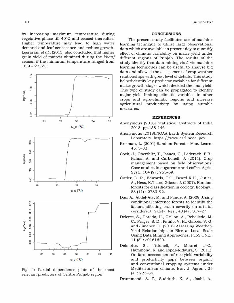
110 June 2020

by increasing maximum temperature during vegetative phase till 40°C and ceased thereafter. Higher temperature may lead to high water demand and leaf senescence and reduce growth. Leerarani et al., (2013) also concluded that higher grain yield of maizeis obtained during the kharif season if the minimum temperature ranged from 18.9 – 22.5°C.

Fig. 4: Partial dependence plots of the most relevant predictors of Centre Punjab region

CoNCLuSIoNSThe present study facilitates use of machine

learning technique to utilize large observational data which are available in present day to quantify effect of climatic variability on maize yield under different regions of Punjab. The results of the study identify that data mining vis-à-vis machine learning techniques can be useful to analyse big data and allowed the assessment of crop-weather relationships with great level of details. This study helpedidentify key predictor variables for different maize growth stages which decided the final yield. This type of study can be propagated to identify major yield limiting climatic variables in other crops and agro-climatic regions and increase agricultural productivity by using suitable measures.

reFereNCeSAnonymous (2018) Statistical abstracts of India

2018, pp.138-146Anonymous (2018).NOAA Earth System Research

Laboratory. https://www.esrl.noaa. gov.Breiman, L. (2001).Random Forests. Mac. Learn.

45: 5–32. Cock, J., Oberthür, T., Isaacs, C., Läderach, P.R.,

Palma, A. and Carbonell, J. (2011). Crop management based on field observations: Case studies in sugarcane and coffee. Agric. Syst., 104 (9) : 755–69.

Cutler, D. R., Edwards, T.C., Beard K.H., Cutler, A., Hess, K.T. and Gibson J. (2007). Random forests for classification in ecology. Ecology., 88 (11) : 2783–92.

Das, A., Abdel-Aty, M. and Pande, A. (2009).Using conditional inference forests to identify the factors affecting crash severity on arterial corridors.J. Safety. Res., 40 (4) : 317–27.

Delerce, S., Dorado, H., Grillon, A., Rebolledo, M. C., Prager, S. D., Patiño, V. H., Garcés. V. G. and Jiménez. D. (2016).Assessing Weather-Yield Relationships in Rice at Local Scale Using Data Mining Approaches. PLoS ONE., 11 (8) : e0161620.

Delmotte, S., Tittonell, P., Mouret, J-C., Hammond, R. and Lopez-Ridaura, S. (2011). On farm assessment of rice yield variability and productivity gaps between organic and conventional cropping systems under Mediterranean climate. Eur. J. Agron., 35 (4) : 223–36.

Drummond, S. T., Sudduth, K. A., Joshi, A.,

Birrell, S. J. and Kitchen, N. R. (2003).Statistical and neural methods for site specific yield prediction. Transact. ASAE., 46 (1) :5–14.

FAO (2017). Food and Agriculture Organization of the United Nations. FAOSTAT Statistical Database. www.fao.org/faostat/en/

Hungerford, R.D., Nemani, R.R., Running, S.W. and Coughlan, J.C. (1989).MTCLIM: amountain microclimate simulation model. U.S. Forest Service Intermountain Resarch Station Research Paper Int-414. Ogden, UT.

Jeong, J. H., Resop, J. P., Mueller, N. D., Fleisher, D. H., Yun, K., Butler, E. E., Timlin, D. J., Shim, K-M., Gerber, J. S., Reddy, V. R. and Kim, S-H. (2016). Random Forests for Global and Regional Crop Yield Predictions.PLoS ONE., 11 (6) : e0156571.

Leelarani, P., Sreenivas, G. and Reddy, D. R. (2013). Evaluating contribution of weather to growth and yield of kharif maize (Zea mays L.) under irrigated conditions.J. Agrometeorology.15 (2) : 156-158

Oguntunde, P. G., Lischeid, G. and Dietrich, O. (2018). Relationship between rice yield and climate variables in southwest Nigeria using multiple linear regression and support vector machine analysis.Int. J. Biometeorol.,

62 (3): 459–69.Pons, M., Marroni, S., Machado, I. and Ghattas,

B. (2009). Machine learning procedures: an application to by-catch data of the marine turtles CarettaCaretta. Collect. Vol. Sci. Pap., 64 (7) : 2443–54.

Schlenker, W. and Roberts, M. J. (2009). Nonlinear temperature effects indicate severe damages to U.S. crop yields under climate change. PNAS., 106:15594–8.

Shmueli G. (2010). To Explain or to Predict? Stat. Sci. 25 (3) : 289–310.

Singh, P., Kumar, S. and Dadhich, S. (2017).Impact of climate variability on the production and productivity of maize (Zea mays l) in north western Himalayan region, India.J. Agrometeorology.19: (Special Issue - AGMET 2016) : 338-44

Strobl, C., Boulesteix, A., Kneib, T., Augustin, T. and Zeileis, A. (2008).Conditional variable importance for random forests. BMC Bioinfo. 9: 307

Tao, F., Yokozawa, M., Hayashi, Y. and Lin, E. (2003). Future climate change, the agricultural water cycle, and agricultural production in China. Agric. Ecosyst. Environ., 95: 203-215.


heat unit requirement and radiation use efficiency of Wheat Cultivars under agroforestry Systems in Northern India

NavNeet Kaur*, KK gILL, BaLJIt SINgh, rIS gILL aNd Bhadra ParIJaPunjab Agricultural University, Punjab-141004*Corresponding Author email - navik20pau.edu

aBStraCtThis study was aimed to determine various agroclimatic indices affecting the growth pattern and yield of wheat cultivars intercropped under 2 and 3 years old poplar and Melia plantations established at a spacing of 8 x 2.5 m and 7 x 3 m, respectively. The cv. PBW 725 accumulated growing degree days 1463, 1434, 1348OC dayunder all the three environments, i.e. open, poplar and Melia block plantations, respectively. Similarly, accumulated photo-thermal units (PTU) were 15765, 15446 and 14594OC day hr for open, poplar and Melia, respectively. The cv. HD 2967 and PBW 725 recorded higher dry matter accumulation and grain yield with 2 and 3 year old poplar and Melia trees, respectively than rest other cultivars. The PBW 725 recorded a significantly highest grain yield HUE under open condition (3.9 kg/ha/0C/day) as compared to under poplar (3.5 kg/ha/0C/day) and Melia (3.6 kg/ha/0C/day) plantation during 2014-15. The regression relationships between radiation use efficiency (RUE) and leaf area index (LAI) of wheat crop was worked out under all the three environments. The coefficient of determination explained better relationship under poplar than Melia plantation in both the years.

Keywords: Agro forestry, wheat cultivars, heat units, RUE

INtroduCtIoN

Forests cover 31 and 21.67 percent of the world and India’s land surface, respectively (FSI, 2019). According to National Forest Policy 1988, one-third (33.3 percent) of the land area should be under forest cover for a sound ecological balance. But the possibility to divert the fertile agricultural land to forests in the view of prevailing socio-economic and agro-climatic conditions is meagre. The only solution for increasing the area under tree cover is integration of trees with crops on farm lands i.e. agroforestry. Deciduous trees have a considerable potential for integration into agroforestry as they shed their leaves, thus allowing resource use by adjacent or under storey crops with minimal interference. Moreover, tree-crop combinations have been found to be more economical than tree or annual crops alone (Burgess et al., 2000; Dhyani et al., 2009). There are many sustainable systems like poplar (Populus deltoides), eucalyptus (Eucalyptus spp.) and Melia (Melia composita) based agroforestry systems. Several research workers from different parts of the country (Roy and Gill, 1990; Gill et al., 2009) have reported good performance of agricultural crops during rabi season viz. wheat, oats, potato, berseem (fodder), mustard, marigold, leafy vegetables, medicinal and spice crops under poplar and Melia species.

In terms of wheat production, India ranks second after China, together contributing 30 per cent of total wheat production of the world and 67 per cent of Asia (Tang et al., 2013) with the northern plains of India comprising the states of Uttar Pradesh, Bihar, Punjab and Haryana contribute 90 per cent of total wheat production in the country. Many researchers have studied performance of various wheat cultivars intercropped under the block plantation of poplar (Chauhan and Dhiman 2007; Gill et al., 2009), however such information under Melia block plantation is limited (Kaur et al., 2017).

The climatic parameters viz., rainfall, light and temperature are vital for optimum crop growth and development which expresses the full crop potential. Out of these three, temperature has a most important role in all the biological functions of crop plants (Girijesh et al., 2011).Several researchers (Kaur et al., 2017; Singh et al., 2017; Singh et al., 2019) reported the effect of microclimatic parameters i.e. air temperature, relative humidity and photosynthetic active radiation (PAR) on physiology and yield of intercrops viz. wheat, turmeric, potato planted under poplar and melia. There is dire need to study the microclimate of crops under the tree canopy because crops and trees compete for bio-resources.


Changes in temperature play a crucial role in determining crop productivity (Fiscus et al., 1997). Decline in potential yield of wheat is linked to negative trend in solar radiation and an increase in minimum temperature under the Indo-Gangetic plains of India (Pathak et al., 2003). The present study was conducted to investigate the microclimatic conditions along with the agroclimatic indices of different wheat cultivars under the tree canopies to provide insights into possible changes in growth patterns and yield of wheat grown under poplar and Melia based plantations.

MaterIaL aNd MethodSDescription of experiment

The research study was carried out under Poplar and Melia plantations which were established during 2012 at the Research Area of the Department of Forestry & Natural Resources, Punjab Agricultural University, Ludhiana. The experimental site is located at longitude of 75°52’E and latitude of 30°54’N and mean sea level height of 247 m.

Poplar and Melia trees were planted at a spacing of 8 x 2.5 m and 7 x 3 m, respectively, with wide strip in the north-south direction. The area between the tree rows was used to sow wheat cultivars during 2013-2014 and 2014-2015. The age of poplar and Meliaplantation during these years was 2 and 3 years, respectively. Wheat cultivars viz., WH 1105, PBW 621, PBW 502, PBW 550, HD 2967 were intercropped with 2 year old poplar and Melia trees during 2013-14 while in the subsequent year PBW 502 and PBW 621 were replaced with newly released high yielding cultivars by the university i.e. PBW 725 and PBW 677.

Experimental design and statistical analysisThe experimental design used was Split Plot

Design with four replications. The data taken was analysed by using ANOVA technique (Panse and Sukhatme, 1985) using CPCS1 software developed by Department of Statistics, Punjab Agricultural University. The means of thetreatments were separated using least significant difference (LSD) test at 5 per cent level of significance.

Crop and Tree managementRegular pruning of these poplar and Melia

plants were done when the trees are leafless (dormant season) in all the years in order to get a maximum volume of excellent quality

knot free timber. Different wheat varieties were also sownin open area in close proximity to the block plantations. The management of the agro forestry area was same way as that of the open i.e. applying recommended fertiliser dose, fungicides, insecticides and irrigation. Wheat cultivars were sown using seed-cum-fertiliser drill in rows 22.5 cm apart (seed rate of 100 kg ha-1). Urea @ 250 kg and DAP @ 125 kg were applied in two splits (half dose of N and full dose of P at the time of sowing and remaining half dose of N after first irrigation). Total 4-5 irrigations were given to the both the plantations during the wheat-growing season every year.

Data collectionThe diameter and height of all the trees in

the experimental plots were measured with the help of diameter tape and Ravi’s Multimeter, respectively each year in March when there is a complete leaf shade. The data of light was taken from ten different points randomly under the plantation at 15 days interval, thrice a day with the help of lux metre having 80 cm long light sensor (Luxmet-300 EXD5) during the entire wheat growing period in between 12 noon to 2 pm. For comparison purpose the light data from the control area (open) was also recorded. The data on various growth parameters viz., plant height, dry matter accumulation, leaf area index {LAI; with Canopy Analyser (LICOR-make) } and photo synthetically active radiations (PAR; with Line Quantum Sensor) were recorded periodically and at harvest stage. For estimating the dry matter accumulation plants from 0.5 m row length were randomly selected from the marked area. Then these plants were cut just above the soil surface at 40, 55, 70, 85, and 100 days. Then the samples taken were sun-dried followed by drying in a hot air oven at 70°C till we get a constant weight in order to estimate dry matter accumulation. The yield attributing characters like tiller number, ear length and 100-grain weight were all recorded at the harvesting time of the wheat. The above ground biomass of all the plants harvested from the plots was recorded. Then the samples were threshed in order to get the grain yield on kg ha-1 basis.

The agrometeorological parameters are calculated using these formulas-

i) Growing Degree Days (GDD) - They are defined as the number of degrees the average daily temperature exceeds a base temperature.


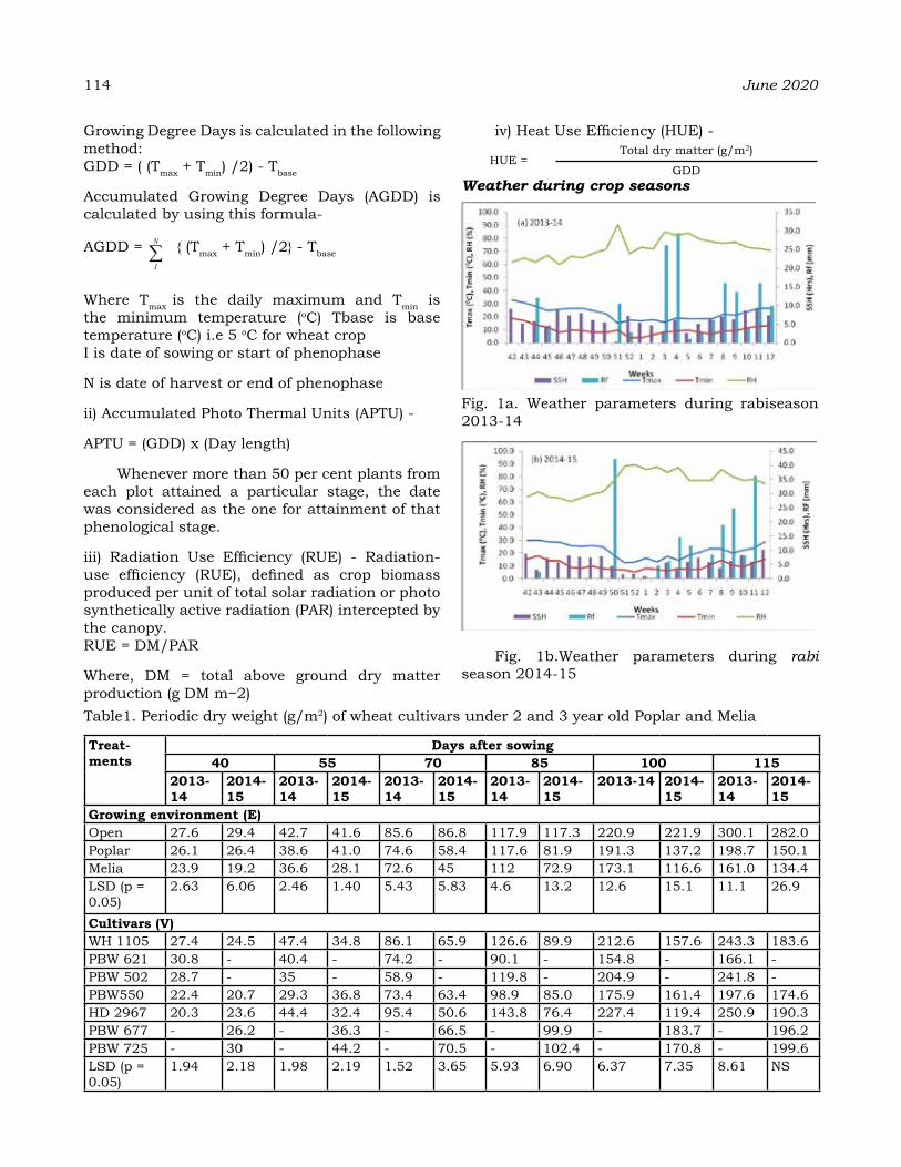
114 June 2020

Growing Degree Days is calculated in the following method:GDD = ( (Tmax + Tmin) /2) - Tbase

Accumulated Growing Degree Days (AGDD) is calculated by using this formula-

AGDD = ∑N

I

{ (Tmax + Tmin) /2} - Tbase

Where Tmax is the daily maximum and Tmin is the minimum temperature (oC) Tbase is base temperature (oC) i.e 5 oC for wheat cropI is date of sowing or start of phenophase

N is date of harvest or end of phenophase

ii) Accumulated Photo Thermal Units (APTU) -

APTU = (GDD) x (Day length)

Whenever more than 50 per cent plants from each plot attained a particular stage, the date was considered as the one for attainment of that phenological stage.

iii) Radiation Use Efficiency (RUE) - Radiation-use efficiency (RUE), defined as crop biomass produced per unit of total solar radiation or photo synthetically active radiation (PAR) intercepted by the canopy.RUE = DM/PAR

Where, DM = total above ground dry matter production (g DM m−2)

iv) Heat Use Efficiency (HUE) -

HUE =Total dry matter (g/m2)

GDDWeather during crop seasons

Fig. 1a. Weather parameters during rabiseason 2013-14

Fig. 1b.Weather parameters during rabi season 2014-15

Table1. Periodic dry weight (g/m2) of wheat cultivars under 2 and 3 year old Poplar and Melia

treat-ments

days after sowing40 55 70 85 100 115

2013-14

2014-15

2013-14

2014-15

2013-14

2014-15

2013-14

2014-15

2013-14 2014-15

2013-14

2014-15

growing environment (e) Open 27.6 29.4 42.7 41.6 85.6 86.8 117.9 117.3 220.9 221.9 300.1 282.0Poplar 26.1 26.4 38.6 41.0 74.6 58.4 117.6 81.9 191.3 137.2 198.7 150.1Melia 23.9 19.2 36.6 28.1 72.6 45 112 72.9 173.1 116.6 161.0 134.4LSD (p = 0.05)

2.63 6.06 2.46 1.40 5.43 5.83 4.6 13.2 12.6 15.1 11.1 26.9

Cultivars (v) WH 1105 27.4 24.5 47.4 34.8 86.1 65.9 126.6 89.9 212.6 157.6 243.3 183.6PBW 621 30.8 - 40.4 - 74.2 - 90.1 - 154.8 - 166.1 -PBW 502 28.7 - 35 - 58.9 - 119.8 - 204.9 - 241.8 -PBW550 22.4 20.7 29.3 36.8 73.4 63.4 98.9 85.0 175.9 161.4 197.6 174.6HD 2967 20.3 23.6 44.4 32.4 95.4 50.6 143.8 76.4 227.4 119.4 250.9 190.3PBW 677 - 26.2 - 36.3 - 66.5 - 99.9 - 183.7 - 196.2PBW 725 - 30 - 44.2 - 70.5 - 102.4 - 170.8 - 199.6LSD (p = 0.05)

1.94 2.18 1.98 2.19 1.52 3.65 5.93 6.90 6.37 7.35 8.61 NS

The data on weather parameters (Fig. 1 a & b) had shown that the year 2013-14 was more favourable for crop growth and yield as compared to 2014-15. During 2013-14, both the temperatures were favourable for the crop growth resulting in better yield during first crop year. In addition, during first crop year more sunshine hours recorded during tillering stage also resulted in good number of tillers while during second year the lower sunshine hours were recorded during early stages of the crop. On the other hand, more than normal rainfall recorded at physiological maturity during 2014-15 in comparison to 2013-14 negatively impacted the crop yield.

reSuLtS aNd dISCuSSIoNPeriodic Dry Weight

The effect on periodic dry weight (gm-2) was evaluated for different wheat cultivars sown in open and intercropped with poplar and Meliaat an interval of 15 days starting from 40 DAS (Table 1). During both years, crop sown under open showed significantly higher dry matter production under all the stages followed by poplar and Melia. There was 40.3 and 49.4 per cent reduction (averaged over two years) in wheat dry matter at 115 days after sowing under poplar and Melia plantations, respectively. This may be attributed to lesser availability of nutrients and moisture under tree plantations. However, the major limiting factor is the shade under trees. Reduced interception of

PAR under plantations becomes one of the most limiting factors ultimately leading to the decline in growth of wheat intercropped under agroforestry systems (Kaur et al., 2016; Singh et al., 2017; Virk et al., 2017). Radiation is one of the basic meteorological parameters which plays role of a decisive factor for crop growth and development ultimately influencing the biological and economic yield of the crop (Lunagaria and Shekh, 2007). In case of wheat, cultivars PBW 725 followed by PBW 667 performed better than rest of the cultivars.

Biometric parameters at harvestPlant height, tiller number, spike length,

grains/spike and 100-grain weight of wheat during 2013-14 and 2014-15 in open and shade conditions were recorded at the time of harvesting and their ANOVA is presented in table 2.

Plant height and tiller numberWith respect to the plant height of wheat

under different microenvironments a non-significant difference was observed in 2013-14 but it varied significantly during 2014-15. Among the different wheat cultivars, there was significant difference in the plant height in the year 2013-14. But the interaction effect between the growing environment and the cultivars did not show any significant difference in the plant height during 2013-14.

Significant difference in the number of tillers

Table 2: Analysis of variance of effect of growing environments and different cultivars on tiller height (TH; cm), tiller number/m row length (TN), spike length (SL; cm), grains/spike (GS), 100 grain weight (GW; g) of wheat crop evaluated during 2013-14 and 2014-15

Source of varia-

tion

dF# th tN SL gS gW2013-

142014-

152013-

142014-15 2013-

142014-

152013-

142014-

152013-

142014-

15Mean squaresReplica-tions

2 21.6ns 83.4ns 58.1ns 189.6ns 0.14ns 0.30 ns 2.15ns 16.9ns 0.44ns 0.56ns

Growing environ-ment (E)

2 90.0ns 312.5* 539.6* 276.4* 1.18* 1.84ns 166.6* 77.1* 0.86ns 3.01*

Error a 4 27.1 32.2 51.2 6.04 0.026 1.20 8.02 9.18 0.16 0.35Culti-vars (V)

4 156.3* 42.3* 36.2ns 106.2* 0.38* 0.06 ns 15.7 ns 3.62 ns 0.17* 1.40*

E X V 8 56.9ns 82.7* 33.4ns 58.3* 0.44* 0.51* 22.2* 40.5* 0.11* 1.85*Error b 24 55.6 42.4 38.3 15.6 0.02 0.14 8.06 12.6 0.03 0.92CV (%) 7.63 7.21 6.49 4.08 1.89 4.13 6.50 7.97 4.28 4.83

*Significant at p<0.05 ; ns, not significant at p<0.05; DF# = Degrees of freedom


116 June 2020

was recorded during both the growing seasons under different growing environments whereas non-significant difference was observed in the tiller numbers of different wheat cultivars in 2013-14 but they did vary significantly in 2014-15. Similar trend was observed in case of the interaction effect between the growing environment and the cultivars. Mcmaster et al., (1987) reported that there is a higher tiller mortality leading to lesser spikes per plant due to shading (50 per cent of ambient light) from booting to one week after anthesis. Similar observations were recorded by Kemp and Whingwiri (1980) who concluded that 20 percent shading of full sunlight before anthesis results in decrease in tiller number. Along withlesser light intensity, leaf litter production from trees also reduces the crop germination and subsequently the growth and developmental parameters. Gill et al., (2009) observed that at the early stage, Poplar has less harmful effect on the alley crops but as the trees grow big and due to more production of leaf litter, the negative effect of trees on crops significantly increased. But difference in the yield and effective tillers in wheat cultivars due to heterogeneity in genetic constitution has also been reported by Rawat et al., (2000).

Yield contributing parametersThe length of the spikes differed significantly

in 2013-14 under different growing conditions as well as among the different cultivars but non-significant difference was observed under both the cases in 2014-15. But the spike length did vary significantly under the interaction effect between the growing environment and the wheat varieties in both the years.

Grains per spike varied significantly under the different growing environments as well as their interaction effects under different growing conditions and cultivars varied significantly in both the growing seasons. Whereas it was observed that there was a non-significant difference in the no. of grains per spike in the different wheat cultivars grown in both the years of cultivation.

The interaction effect of the hundred grain weight with that of the different growing environments was found to be significant in both the years of experiment among the different cultivars of wheat. This may be attributed to the decrease in growth and development of crop owing to reduced moisture and nutrient availability under the plantations. Similar findings was also

recorded by Gill et al., (2009). Willey and Holliday (1971) concluded in their study that reduction of 28 to 54 per cent of full light due to shading during the period of ear development leads to a significant decline in number of grains and grain weight per ear.

Grain yieldThe grain yield was significantly higher in

open conditions during both the years than under the treesin all the wheat cultivars (Table 3). Among the trees, the grain yield was found to be higher under Poplar block plantation than under Melia plantation. As the trees also competes with the under canopy agricultural crops for the necessary resources this leads to the reduction in crop yield. The yield of cultivar HD 2967 was higher than other cultivars but at par with WH 1105 and PBW 621 under two year old poplar and Melia. But under three years old plantation of poplar and Melia, PBW 725 out raced all the other cultivars but was statistically at par with PBW 677.

Table 3: Effect of environment ongrain yield of wheat cultivars

treatments grain yield (qha-1) 2013-14 2014-15

growing environment (e) Open 55.4 56.9Poplar 50.2 48.3Melia 46.9 43.7LSD (p=0.05) 4.76 5.34Cultivars (v) WH 1105 51.8 47.9PBW 621 49.2 -PBW 502 49.0 -PBW550 50.5 47.8HD 2967 52.9 49.2PBW677 - 50.3PBW 725 - 51.7LSD (p=0.05) 2.25 2.33

Agroclimatic indices, grain yield and heat use efficiency (HUE)

The different agroclimatic indices and heat use efficiencies were worked out under different environments. Different cultivars of wheat utilized different agroclimatic indices to attain physiological maturity. During the year 2013-14, among the different wheat cultivars, WH1105 accumulated the highest growing degree days (AGDD) of 1483oC day, which was obtained under

open conditions followed by Melia plantation (1418oC day) and Poplar block plantation (1345oC day). Accumulated photothermal units (APTU) also followed the similar trend as that of growing degree days. In general daylength is not affecting the microclimate directly but it is indirectly affecting through growing degree days. So, APTU had also decreased from 16085oC day hr under open conditions to 15618oC day hr and 14721oC day hr for Meliaplantation and Poplar block plantation, respectively. Maximum grain yield was observed for the wheat cultivar HD 2967 (5673, 5247, 5203 kg ha-1) in open, under Meliaand Poplar block plantation, respectively.Highest grain yield HUE of 3.9 kg ha-1°C day-1 (cv. WH 1105) was recorded in open conditions; 3.9 kg ha-1°C day-1 (WH 1105 and HD 2967) under Poplar block plantation and 3.7 kg ha-1°C day-1 (HD 2967) under Meliaplantation.

During the year 2014-15, highest value of growing degree days was recorded for the cultivar PBW 725 (14630C day) followed by Poplar block plantation (14340C day) and Melia plantation (13480C day). Similar trend was obtained for APTU i.e. maximum for the wheat cultivar PBW 725 when planted in open condition (157650C day hr) followed by Poplar block plantation (15446oC day hr) and Meliaplantation (145940C day hr). Maximum grain yield of 5740 kg/ha was observed for the wheat cultivars PBW 725 when planted

under open conditions and lowest for WH 1105 under Meliaplantation (3920 kg ha-1).Highest grain yield HUE of 4.0 kg ha-1 °C day-1 (PBW 725) was recorded in open conditions followed by under Melia plantation (3.8 kg ha-1°C day-1 ) andunder Poplar block plantation 3.4 kg ha-1°C day-1 (HD 2967 and PBW 725). Similar comparative studies were also worked out under different environments by Gill et al., (2016) and Singh et al., (2017). The thermal unit requirement decreased under shade conditions because of less accumulation of heat units which are most essential for crop growth and development. Although crop duration increases under shade conditions but heat units requirement is not fulfilled resulting in lower yield than open.

Relationship between leaf area index (LAI) and radiation use efficiency (RUE)

The radiation use efficiency of crops is mostly a resultof the fraction of the incoming photosynthetically active radiation intercepted by the canopy, is a function of leaf area index and its efficiency to intercepts solar radiation (Sandana et al., 2009). Dry matter production is often observed to be in a linear relationship to the intercepted photosynthetically active radiation (PAR) by the crops and radiation use efficiency (RUE) is the slope of this relationship which is used as a means to correlate with that of the plant growth (Mukherjee et al., 2014). Regression

Table 4: Accumulated growing degree days (AGDD), accumulated photothermal units (APTU) and heat use efficiency (HUE) of wheat cultivars under open and shade conditions during 2013-14

environment Cultivars agdd (°C day) aPtu (°C day hr)

grain yield (kg ha-1)

grain yield hue (kg ha-1°C day-1)

Open

WH 1105 1466.3 15879.9 5650 3.9PBW 621 1443.1 15587.3 5457 3.8PBW 502 1417.6 15499.3 5413 3.8PBW550 1457.6 15680.6 5523 3.8HD 2967 1483.1 16085.5 5673 3.8

Poplar

WH 1105 1400.5 14497.7 5140 3.7PBW-621 1355.5 14284.3 4867 3.6PBW-502 1338.0 13666.1 4806 3.6PBW 550 1361.0 14505.3 5053 3.7HD-2967 1418.5 14720.6 5247 3.7

Melia

WH 1105 1327.7 15394.9 4750 3.6PBW-621 1307.7 14622.1 4433 3.4PBW-502 1301.1 14600.3 4496 3.5PBW 550 1319.8 14906.7 4563 3.5HD-2967 1345.1 15617.7 5203 3.9


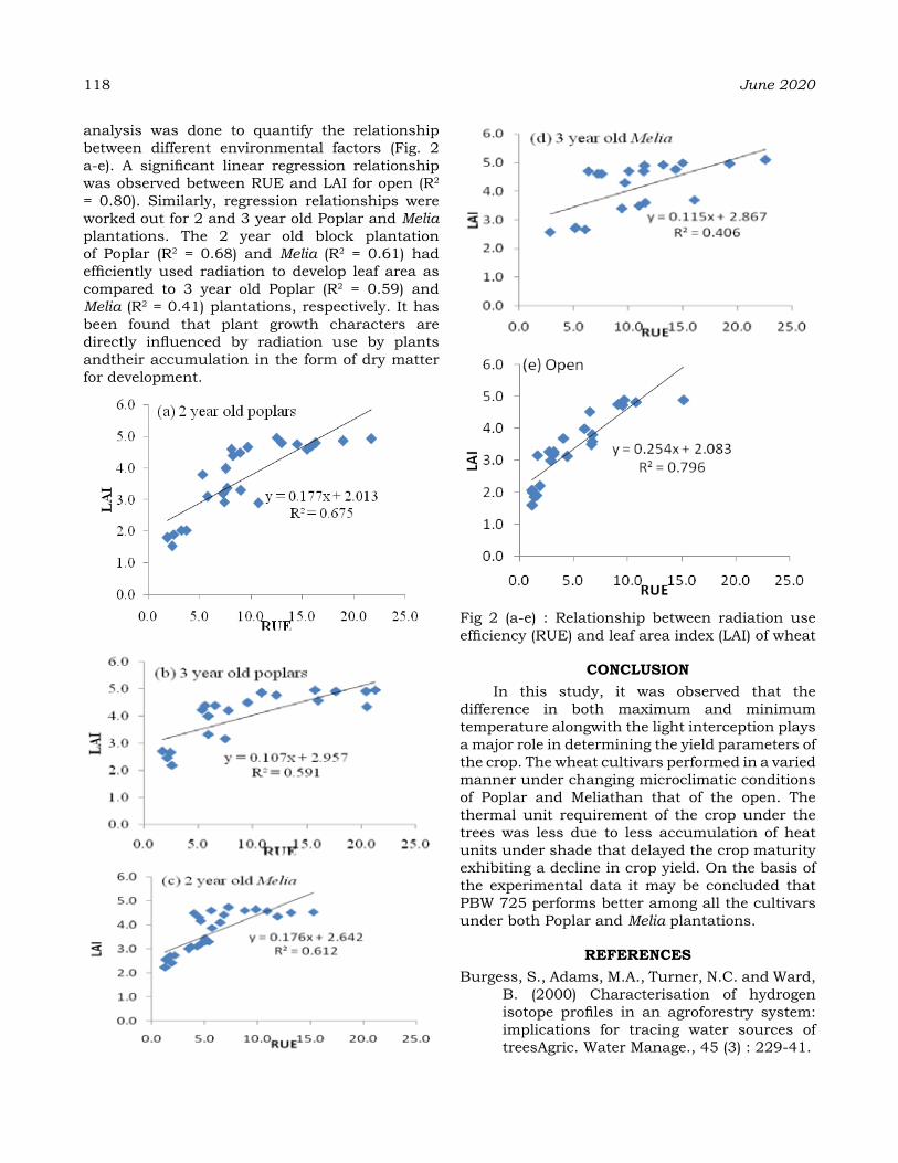
118 June 2020

analysis was done to quantify the relationship between different environmental factors (Fig. 2 a-e). A significant linear regression relationship was observed between RUE and LAI for open (R2 = 0.80). Similarly, regression relationships were worked out for 2 and 3 year old Poplar and Melia plantations. The 2 year old block plantation of Poplar (R2 = 0.68) and Melia (R2 = 0.61) had efficiently used radiation to develop leaf area as compared to 3 year old Poplar (R2 = 0.59) and Melia (R2 = 0.41) plantations, respectively. It has been found that plant growth characters are directly influenced by radiation use by plants andtheir accumulation in the form of dry matter for development.

Fig 2 (a-e) : Relationship between radiation use efficiency (RUE) and leaf area index (LAI) of wheat

CoNCLuSIoNIn this study, it was observed that the

difference in both maximum and minimum temperature alongwith the light interception plays a major role in determining the yield parameters of the crop. The wheat cultivars performed in a varied manner under changing microclimatic conditions of Poplar and Meliathan that of the open. The thermal unit requirement of the crop under the trees was less due to less accumulation of heat units under shade that delayed the crop maturity exhibiting a decline in crop yield. On the basis of the experimental data it may be concluded that PBW 725 performs better among all the cultivars under both Poplar and Melia plantations.

reFereNCeSBurgess, S., Adams, M.A., Turner, N.C. and Ward,

B. (2000) Characterisation of hydrogen isotope profiles in an agroforestry system: implications for tracing water sources of treesAgric. Water Manage., 45 (3) : 229-41.

Table 5: Accumulated growing degree days (AGDD), accumulated photothermal units (APTU) and heat use efficiency (HUE) of wheat cultivars under open and shade conditions during 2014-15

environment Cultivars agdd (°C day) aPtu (°C day hr)

grain yield (kg ha-1)

grain yield hue (kg ha-1°C day-1)

Open

WH 1105 1414 15527 5650 4.0PBW 550 1404 15050 5540 3.9HD 2967 1424 15284 5690 4.0PBW 677 1444 15527 5710 4.0PBW 725 1463 15765 5740 3.9

Poplar

WH 1105 1396 15196 4670 3.3PBW 550 1384 15144 4473 3.2HD 2967 1414 15325 4820 3.4PBW 677 1416 15246 4730 3.3PBW 725 1434 15446 5087 3.5

Melia

WH 1105 1296 14173 3920 3.0PBW 550 1294 14159 4193 3.2HD 2967 1330 14373 4257 3.2PBW 677 1330 14588 4420 3.3PBW 725 1348 14594 4883 3.6

Chaudhry, A.K., Khan, G.S., Siddiqui, M.T., Akhtar, M. and Aslam, Z. (2003) Physico-chemical characteristics of wheat variety Inqalab-91 under Poplar (Populusdeltoides) based agroforestry system. Pak. J. Agric. Sci., 40: 77-81.

Chauhan, V.K. and Dhiman, R.C. (2007) Atmospheric humidity and air temperature studies in wheat-Poplar based agroforestry system. Indian For., 133: 73-78.

Dhyani, S.K., Sharma, A.R. and Niwaz, R. (2009) Agroforestry: Its relation with agronomy, challenges and opportunities. Indian J. Agron., 54 (3) :249-66.

Fiscus, E.L., Reid, C.D., Miller, J.E. and Heagle, A.S. (1997) Elevated CO2 reduces O3 flux and O3-induced yield losses in soybeans: possible implications for elevated CO2 studies. J.Exptal. Bot., 48: 307–13.

FSI (2019) Indian State of Forest Report, published by Forest Survey of India.

Gill, K. K., Kaur, N. and Gill, R. I. S. (2016) Evaluation of growth and yield of wheat cultivars using agroclimatic indices under Poplar basedagroforestry system in Punjab. J.Agrometeorol., 18 (1) : 124-27.

Gill, R.I.S., Singh, B. and Kaur, N. (2009) Productivity and nutrient uptake of newly released wheat varieties at different sowing

times under Poplar plantation in north-western India. Agrofor. Sys., 76 (3) : 579-90.

Girijesh, G.K., Kumara Swamy, A.S., Sreedhar, S., Dinesh Kumar, M., Vageesh, T.S. And Rajashekarappa, K.S. (2011) Heat unit utilization of kharif maize in transitional zone of Karnataka. J.Agrometeorol., 13 (1) : 43-45.

Kaur, N., Singh, B. and Gill, R.I.S. (2017) Productivity and profitability of intercrops under four tree species throughout their rotation in north-western India. Indian J.Agron., 62 (2) :151-159.

Kemp, D.R. and Whingwiri, E.E. (1980) Effect of tiller removal and shading on spikelet development and yield component of the main shoot of wheat and the sugar concentration of the ear and flag leaf. Aust. J. Plant Physiol. 7:501-10.

Lunagaria, M.M. and Shekh, A.M. (2007) Radiation use efficiency of wheat (Triticumaestivum L.) crop as influenced by date of sowing, row spacing and row orientation. J. Agrometeorol., 9 (1) : 282-85.

Mcmaster, G.S., Morgan, J.A. and Willis, W.O. (1987) Effects of shading on winter wheat yield, spike characteristics and carbohydrate allocation.Crop Sci., 27 (5) :967-73.

Mukherjee, J., Singh, G. and Bal, S.K. (2014)


120 June 2020

Radiation use efficiency and instantaneous photosynthesis at different growth stages of wheat (Triticumaestivum L.) in semi arid ecosystem of Central Punjab, India. J. Agrometeorol.16 (1) : 69-77.

Panse, V.G. and Sukhatme, P.V. (1985) Statistical methods for agricultural workers, 4th edn. ICAR, New Delhi, pp 359.

Pathak, H., Prasad, S., Bhatia, A., Singh, S., Kumar, S., Singh, J. and Jain, M. C. (2003) Methane emission from rice-wheat cropping system of India in relation to irrigation, farmyard manure and dicyandiamide application.Agric.Ecosys.Environ., 97: 309-16.

Rawat, A.K., Sharma, R.S., Dubey, A.K. and Naik, K.R. (2000) Refinement of agro-techniques for improving the productivity of wheat (Triticumaestivum) under rice (Oryza sativa) –wheat agro-ecosystem. Indian J.Agron., 45:636-40.

Roy, R.D. and Gill, A.S. (1990) Agroforestry where food is wedded to fuelwood. Indian Far., 40 (7) : 33-38.

Sandaña, P., Harcha, C. I., & Calderini, D. F. (2009). Sensitivity of yield and grain nitrogen concentration of wheat, lupin and pea to source reduction during grain filling.A

comparative survey under high yielding conditions. Field Crops Res., 114: 233–43.

Singh, R., Kaur, N., Gill, K.K. and Gill, R.I.S. (2017) Radiation interception and thermal requirement of wheat cultivars under Burma dek (Meliacomposita Willd.) in central Punjab.J.Agrometeorol.19 (4) : 369-71.

Singh, P., Sharma, S.P., Kaur, N. and Gill, R.I.S. (2019) Potato cultivars differ in response to date of planting in intercrop with Poplar (Populusdeltoides Bartr. ex Marsh.) in irrigated agro-ecosystem of north-west India. Agrofor. Syst., doi.org/10.1007/s10457-019-00356-w, pp 1-11.

Tang, H., Takigawa, M., Liu, G., Zhu, J. and Kobayashi, K. (2013) A projection of ozone-induced wheat production loss in China and India for the years 2000 and 2020 with exposure-based and flux-based approaches.Global Change Biol., 19 (9) : 2609-928.

Virk, J., Gill, R.I.S., Kaur, N., Singh, B. and Singh, R. (2017) Evaluation of wheat varieties under Popular deltoides plantation under various tree spacing. Indian J. Agrofor., 19 (1) : 57-62.

Willey, R.W. and Holliday, R. (1971) Plant population, shading and thining studies in wheat. J. Agric. Sci.Camb., 77:543-61.

Spatial variation of rainfed maize yield response to climate change in tamil Nadu

r. reNgaLaKShMI*, v.geethaLaKShMI** aNd K.BhuvaNeSWarI**

*MS Swaminathan Research Foundation, Chennai - 600 113**Tamil Nadu Agricultural University, Coimbatore - 641003

Corresponding author email: [email protected]

aBStraCtClimate variability and climate change associated with increases in CO2, warming and alterations in rainfall pattern make huge impact on agriculture. The adverse effect of climate change is expected to aggravate in future due to increasing frequency of extreme weather events such as droughts and floods. The aim of the study was to portraythe spatial response of maize productivity under changing climate over Tamil Nadu. For this purpose, HadGEM2-AO general circulation model generated future climate under RCP 4.5 and RCP 8.5 scenarios were used in DSSAT-CERES – Maize crop model. The simulated results of DSSAT-CERES – Maize model showed the marked variation in maize productivity across the different agro climate regions of Tamil Nadu. Among all zones, maize yield varied much in North Western Zone (NWZ) n present climate with the yield variation from 903 to 5254 kg ha-1. The lowest yield variation (2586 to 4957 kg ha -1) was observed in North Eastern Zone (NEZ). Maize productivity is predicted to decline in end century than near and mid century. Cauvery Delta Zone (CDZ) exhibited relatively higher impact on maize productivity by climate change and the yield reduction was less in Western Zone (WZ) of Tamil Nadu.

Keywords: Climate change, RCP, CERES – Maize, spatial variation, Tamil Nadu

INtroduCtIoN

India is home to more than one sixth of the world’s population and primarily an agrarian country. Any variations in the seasonal mean monsoon rainfall determine crop production. Ten percent fluctuation in monsoon rainfall results in flood or drought conditions and consequently leading to adverse impacts on crop productivity. In summary, the monsoon rainfall determines every pulse of Indian agriculture (Gadgil et al., 1996, Ashwini Kulkarni et al., 2016). Greenhouse gasses in the atmosphere have significantly increased relative pre-industrial period that being the majorsource for the warming of atmosphere (IPCC, 2007; Miao et al., 2013). Future impacts are projected to get amplified due to continued rise in temperature and abnormal changes in rainfall pattern (Justus Ochieng et al., 2016). Climate variability and change considerably affects the crop production and are expected to worsen in the future. Maize occupies third place among the cereals after rice and wheat in India. It is grown in an area of 96 lakh ha with the production and productivity of 260 lakh tons and 2710 kg ha-1, respectively (NCoMM, 2016). In Tamil Nadu, it is grown in an area of 3.15 lakh ha with a production

of 9.53 lakh tons and productivity of 3026 kg ha-1 (India stat, 2016).

In India, poultry sector consumes major part of total maize produced (51%) followed by human consumption (26%), starch making (12%) and livestock feeds (11%). Although demand for maize in Asia is huge, India is ideally placed to capitalize on this opportunity now (FICCI, 2018). Hence, there is compelling need to assess the impact of climate change on maize productivity at different regions and explore the potential adaptation strategies for increasing the productivity against climate change.

MaterIaLS aNd MethodSStudy Area

The study was carried in six Agro Climatic Zones (ACZ) out of seven ACZ in Tamil Nadu. As the maize crop isn’t cultivated in hilly zone of Tamil Nadu the remaining zones such as North Eastern Zone (NEZ), North Western Zone (NWZ), Western Zone (WZ), High Rainfall Zone (HRZ), Southern Zone (SZ) and Cauvery Delta Zone (CDZ) were considered for the study (Fig. 1).


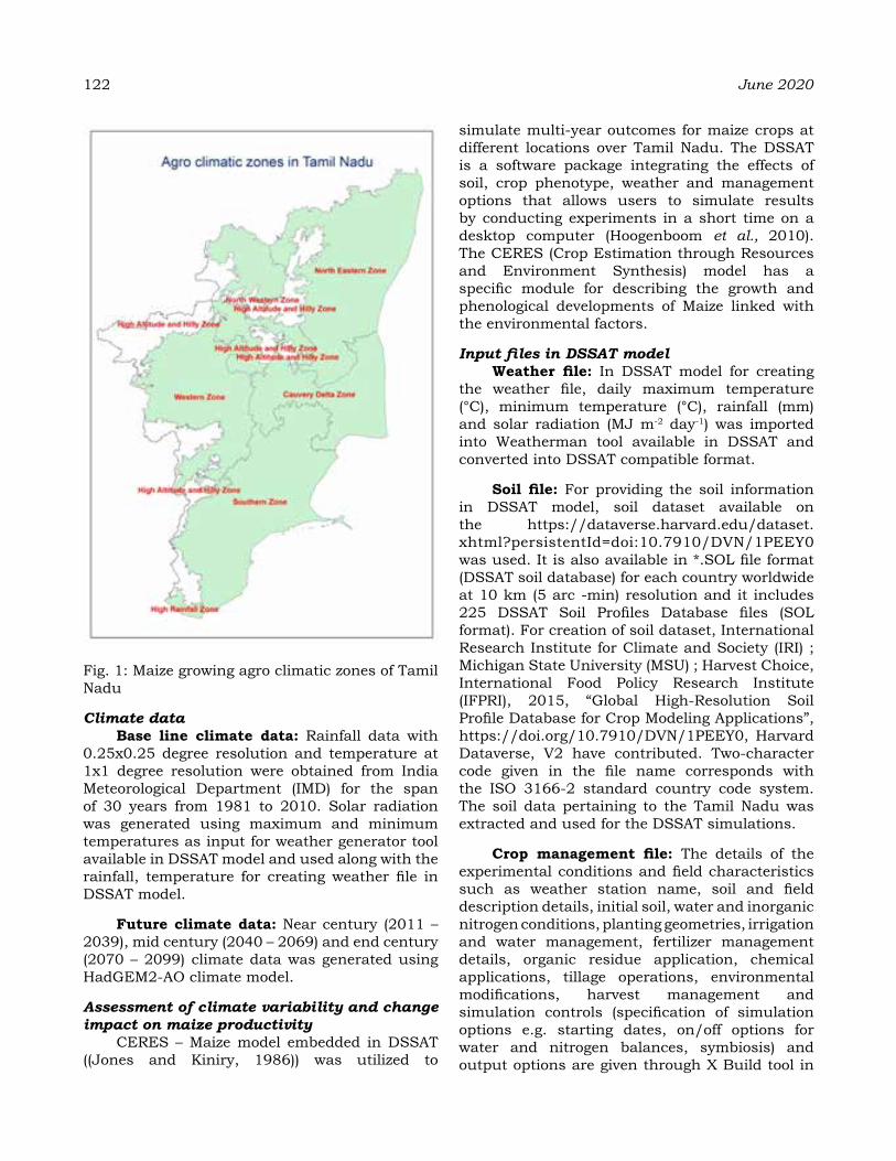
122 June 2020

Fig. 1: Maize growing agro climatic zones of Tamil Nadu

Climate dataBase line climate data: Rainfall data with

0.25x0.25 degree resolution and temperature at 1x1 degree resolution were obtained from India Meteorological Department (IMD) for the span of 30 years from 1981 to 2010. Solar radiation was generated using maximum and minimum temperatures as input for weather generator tool available in DSSAT model and used along with the rainfall, temperature for creating weather file in DSSAT model.

Future climate data: Near century (2011 – 2039), mid century (2040 – 2069) and end century (2070 – 2099) climate data was generated using HadGEM2-AO climate model.

Assessment of climate variability and change impact on maize productivity

CERES – Maize model embedded in DSSAT ((Jones and Kiniry, 1986)) was utilized to

simulate multi-year outcomes for maize crops at different locations over Tamil Nadu. The DSSAT is a software package integrating the effects of soil, crop phenotype, weather and management options that allows users to simulate results by conducting experiments in a short time on a desktop computer (Hoogenboom et al., 2010). The CERES (Crop Estimation through Resources and Environment Synthesis) model has a specific module for describing the growth and phenological developments of Maize linked with the environmental factors.

Input files in DSSAT model Weather file: In DSSAT model for creating

the weather file, daily maximum temperature (°C), minimum temperature (°C), rainfall (mm) and solar radiation (MJ m-2 day-1) was imported into Weatherman tool available in DSSAT and converted into DSSAT compatible format.

Soil file: For providing the soil information in DSSAT model, soil dataset available on the https://dataverse.harvard.edu/dataset.xhtml?persistentId=doi:10.7910/DVN/1PEEY0 was used. It is also available in *.SOL file format (DSSAT soil database) for each country worldwide at 10 km (5 arc -min) resolution and it includes 225 DSSAT Soil Profiles Database files (SOL format). For creation of soil dataset, International Research Institute for Climate and Society (IRI) ; Michigan State University (MSU) ; Harvest Choice, International Food Policy Research Institute (IFPRI), 2015, “Global High-Resolution Soil Profile Database for Crop Modeling Applications”, https://doi.org/10.7910/DVN/1PEEY0, Harvard Dataverse, V2 have contributed. Two-character code given in the file name corresponds with the ISO 3166-2 standard country code system. The soil data pertaining to the Tamil Nadu was extracted and used for the DSSAT simulations.

Crop management file: The details of the experimental conditions and field characteristics such as weather station name, soil and field description details, initial soil, water and inorganic nitrogen conditions, planting geometries, irrigation and water management, fertilizer management details, organic residue application, chemical applications, tillage operations, environmental modifications, harvest management and simulation controls (specification of simulation options e.g. starting dates, on/off options for water and nitrogen balances, symbiosis) and output options are given through X Build tool in

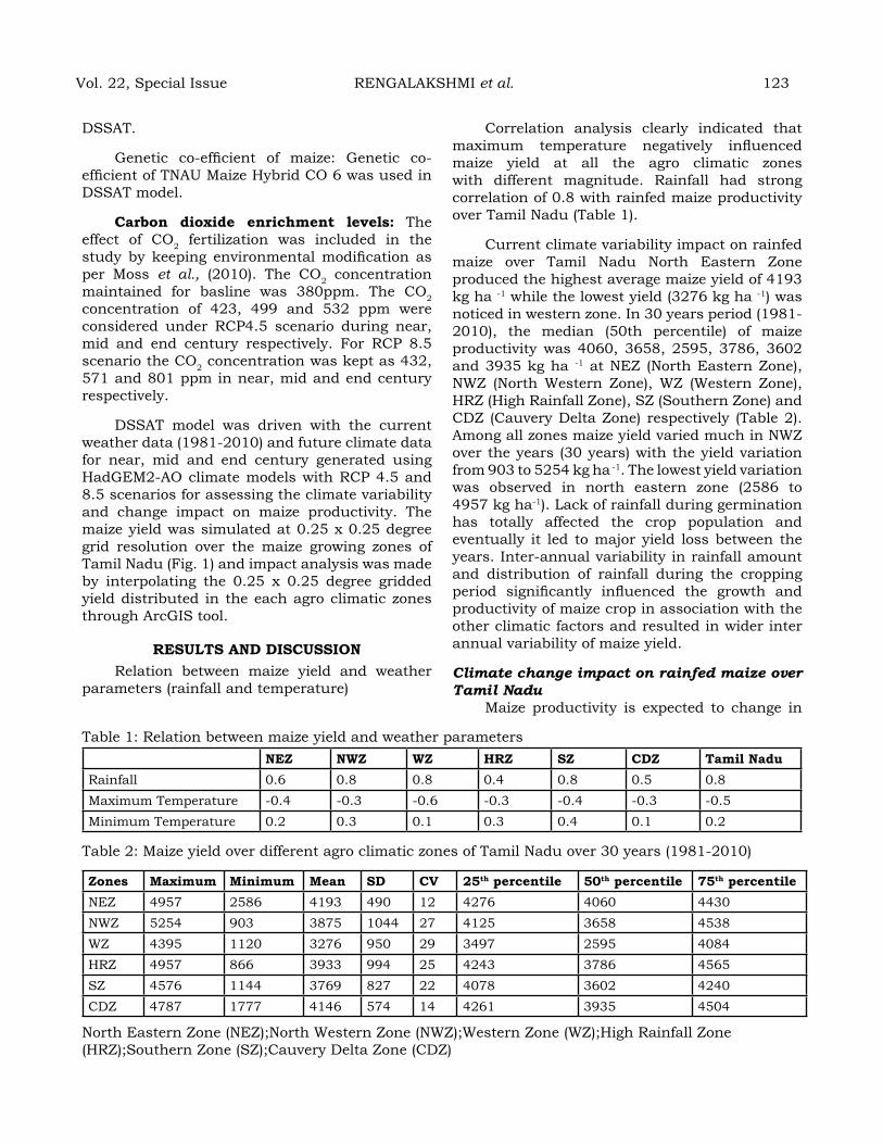
DSSAT.

Genetic co-efficient of maize: Genetic co-efficient of TNAU Maize Hybrid CO 6 was used in DSSAT model.

Carbon dioxide enrichment levels: The effect of CO2 fertilization was included in the study by keeping environmental modification as per Moss et al., (2010). The CO2 concentration maintained for basline was 380ppm. The CO2 concentration of 423, 499 and 532 ppm were considered under RCP4.5 scenario during near, mid and end century respectively. For RCP 8.5 scenario the CO2 concentration was kept as 432, 571 and 801 ppm in near, mid and end century respectively.

DSSAT model was driven with the current weather data (1981-2010) and future climate data for near, mid and end century generated using HadGEM2-AO climate models with RCP 4.5 and 8.5 scenarios for assessing the climate variability and change impact on maize productivity. The maize yield was simulated at 0.25 x 0.25 degree grid resolution over the maize growing zones of Tamil Nadu (Fig. 1) and impact analysis was made by interpolating the 0.25 x 0.25 degree gridded yield distributed in the each agro climatic zones through ArcGIS tool.

reSuLtS aNd dISCuSSIoNRelation between maize yield and weather

parameters (rainfall and temperature)

Correlation analysis clearly indicated that maximum temperature negatively influenced maize yield at all the agro climatic zones with different magnitude. Rainfall had strong correlation of 0.8 with rainfed maize productivity over Tamil Nadu (Table 1).

Current climate variability impact on rainfed maize over Tamil Nadu North Eastern Zone produced the highest average maize yield of 4193 kg ha -1 while the lowest yield (3276 kg ha -1) was noticed in western zone. In 30 years period (1981-2010), the median (50th percentile) of maize productivity was 4060, 3658, 2595, 3786, 3602 and 3935 kg ha -1 at NEZ (North Eastern Zone), NWZ (North Western Zone), WZ (Western Zone), HRZ (High Rainfall Zone), SZ (Southern Zone) and CDZ (Cauvery Delta Zone) respectively (Table 2). Among all zones maize yield varied much in NWZ over the years (30 years) with the yield variation from 903 to 5254 kg ha -1. The lowest yield variation was observed in north eastern zone (2586 to 4957 kg ha-1). Lack of rainfall during germination has totally affected the crop population and eventually it led to major yield loss between the years. Inter-annual variability in rainfall amount and distribution of rainfall during the cropping period significantly influenced the growth and productivity of maize crop in association with the other climatic factors and resulted in wider inter annual variability of maize yield.

Climate change impact on rainfed maize over Tamil Nadu

Maize productivity is expected to change in

Table 1: Relation between maize yield and weather parametersNeZ NWZ WZ hrZ SZ CdZ tamil Nadu

Rainfall 0.6 0.8 0.8 0.4 0.8 0.5 0.8Maximum Temperature -0.4 -0.3 -0.6 -0.3 -0.4 -0.3 -0.5Minimum Temperature 0.2 0.3 0.1 0.3 0.4 0.1 0.2

Table 2: Maize yield over different agro climatic zones of Tamil Nadu over 30 years (1981-2010)

Zones Maximum Minimum Mean Sd Cv 25th percentile 50th percentile 75th percentileNEZ 4957 2586 4193 490 12 4276 4060 4430NWZ 5254 903 3875 1044 27 4125 3658 4538WZ 4395 1120 3276 950 29 3497 2595 4084HRZ 4957 866 3933 994 25 4243 3786 4565SZ 4576 1144 3769 827 22 4078 3602 4240CDZ 4787 1777 4146 574 14 4261 3935 4504

North Eastern Zone (NEZ);North Western Zone (NWZ);Western Zone (WZ);High Rainfall Zone (HRZ);Southern Zone (SZ);Cauvery Delta Zone (CDZ)

Vol. 22, Special Issue RENGALAKSHMI et al. 123

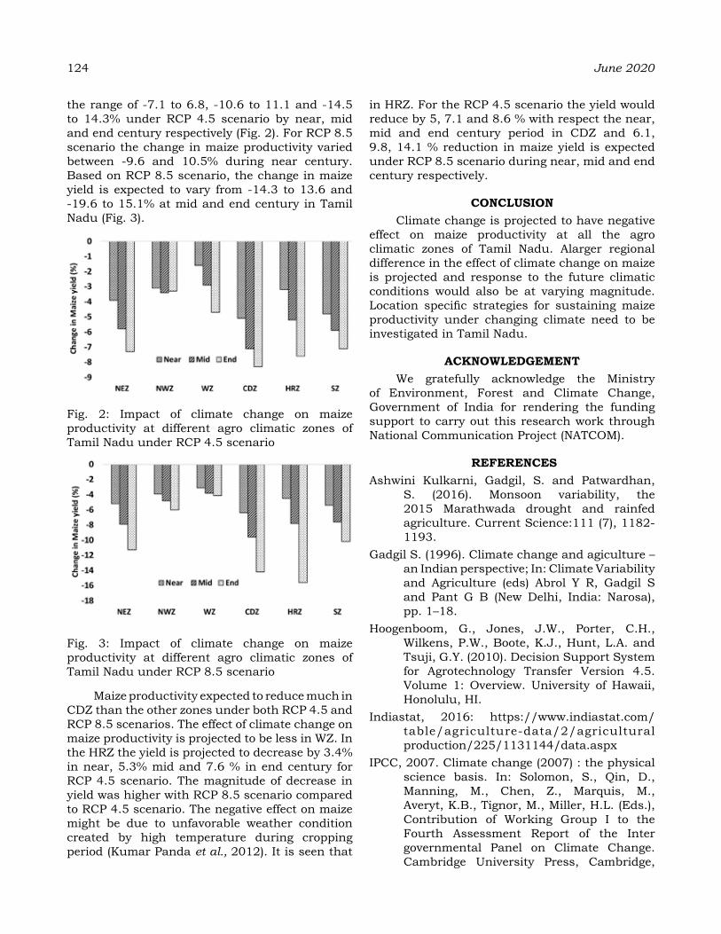
124 June 2020

the range of -7.1 to 6.8, -10.6 to 11.1 and -14.5 to 14.3% under RCP 4.5 scenario by near, mid and end century respectively (Fig. 2). For RCP 8.5 scenario the change in maize productivity varied between -9.6 and 10.5% during near century. Based on RCP 8.5 scenario, the change in maize yield is expected to vary from -14.3 to 13.6 and -19.6 to 15.1% at mid and end century in Tamil Nadu (Fig. 3).

Fig. 2: Impact of climate change on maize productivity at different agro climatic zones of Tamil Nadu under RCP 4.5 scenario

Fig. 3: Impact of climate change on maize productivity at different agro climatic zones of Tamil Nadu under RCP 8.5 scenario

Maize productivity expected to reduce much in CDZ than the other zones under both RCP 4.5 and RCP 8.5 scenarios. The effect of climate change on maize productivity is projected to be less in WZ. In the HRZ the yield is projected to decrease by 3.4% in near, 5.3% mid and 7.6 % in end century for RCP 4.5 scenario. The magnitude of decrease in yield was higher with RCP 8.5 scenario compared to RCP 4.5 scenario. The negative effect on maize might be due to unfavorable weather condition created by high temperature during cropping period (Kumar Panda et al., 2012). It is seen that

in HRZ. For the RCP 4.5 scenario the yield would reduce by 5, 7.1 and 8.6 % with respect the near, mid and end century period in CDZ and 6.1, 9.8, 14.1 % reduction in maize yield is expected under RCP 8.5 scenario during near, mid and end century respectively.

CoNCLuSIoNClimate change is projected to have negative

effect on maize productivity at all the agro climatic zones of Tamil Nadu. Alarger regional difference in the effect of climate change on maize is projected and response to the future climatic conditions would also be at varying magnitude. Location specific strategies for sustaining maize productivity under changing climate need to be investigated in Tamil Nadu.

aCKNoWLedgeMeNt We gratefully acknowledge the Ministry

of Environment, Forest and Climate Change, Government of India for rendering the funding support to carry out this research work through National Communication Project (NATCOM).

reFereNCeSAshwini Kulkarni, Gadgil, S. and Patwardhan,

S. (2016). Monsoon variability, the 2015 Marathwada drought and rainfed agriculture. Current Science:111 (7), 1182-1193.

Gadgil S. (1996). Climate change and agiculture – an Indian perspective; In: Climate Variability and Agriculture (eds) Abrol Y R, Gadgil S and Pant G B (New Delhi, India: Narosa), pp. 1–18.

Hoogenboom, G., Jones, J.W., Porter, C.H., Wilkens, P.W., Boote, K.J., Hunt, L.A. and Tsuji, G.Y. (2010). Decision Support System for Agrotechnology Transfer Version 4.5. Volume 1: Overview. University of Hawaii, Honolulu, HI.

Indiastat, 2016: https://www.indiastat.com/table/agriculture-data/2/agricultural production/225/1131144/data.aspx

IPCC, 2007. Climate change (2007) : the physical science basis. In: Solomon, S., Qin, D., Manning, M., Chen, Z., Marquis, M., Averyt, K.B., Tignor, M., Miller, H.L. (Eds.), Contribution of Working Group I to the Fourth Assessment Report of the Inter governmental Panel on Climate Change. Cambridge University Press, Cambridge,

United Kingdom and New York NY.Jones, C. A and J. R. Kiniry. 1986. CERES-Maize:

A Simulation Model of Maize Growth and Development. Texas A & M University Press, College Station, Texas.

Justus Ochieng, Lilian Kirimi, Mary Mathenge. (2016). Effects of climate variability and change on agricultural production: The case of small scale farmers in Kenya, NJAS - Wageningen Journal of Life Sciences. 77:71-78

Kumar Panda, R., J. Alam and S. Nandgude. 2012. Effect of climate variability on maize yield and evaluation of coping strategies using the crop growth model. Intl. J. Climate Change Impact Res., 3 (2) :71-94.

Miao, C.Y., Duan, Q.Y., Sun, Q.H. and Li, J.D. (2013). Evaluation and application of bayesian multi-model estimation in

temperature simulations Prog. Phys. Geog. 37: 727–744.

Moss, R.H., J.A. Edmonds, K.A. Hibbard, M.R. Manning, S.K. Rose, D.P. Van Vuuren, T.R. Carter, S. Emori, M. Kainuma, T. Kram, G.A. Meehl, J.F.B. Mitchell, N. Nakicenovic, K. Riahi, S.J. Smith, R.J. Stouffer, A.M. Thomson, J.P. Weyant and T.J. Wilbanks. 2010. The next generation of scenarios for climate change research and assessment. Nature, 463: 747-756.

National Collateral Management Services Limited (NCoMM). 2016. http://www.ncml.com/Upload/ New/ Pdf/ c7495fab-54d7-4b03-a04a-47c2da337039.pdf

The Federation of Indian Chambers of Commerce and Industry (FICCI). Maize Vision 2022. A Knowledge Report. 2018.pg 1-86.

Vol. 22, Special Issue RENGALAKSHMI et al. 125

response of Pomegranate (Punica granatum L.) to deficit irrigation systemunder field conditions.

d.t. MeShraM1, K.d.BaBu1, a.K. NaIr2, P. PaNIgrahI3 aNd S.S. WadNe1

1-ICAR-National Research Center on Pomegranate, Solapur-413255, Maharashtra, India.2-ICAR-Indian Institute of Horticulture Research, Bengaluru-560 089, Karnataka, India3-ICAR-Indian Institute of Water Management, Bhubaneshwar-751 023, Odisha, India

Corresponding author [email protected]

aBStraCtA field experiment was carried out from September, 2015 to April, 2019 in Hastabahar at Solapur (i.e. 170 10’’, 740 42’’ and 483.5 m msl) to evaluate the effect of deficit irrigation strategies on growth, fruit quality parameters, yield and water use efficiency in pomegranate orchards. Each respective year of six treatments (20 to 100 % * ETp) for 3-6 year old pomegranate trees were undertaken. The results showed that, less water produce good performance of vegetative growth, no water shoot and luxur. Reduced moisture content and maximum plant height, branches, LAI and plant spread is recorded at 100%*ETp, however yield and water use efficiency is observed at 40 to 70%*ETr. The moisture content and relative leaf water content in % age varies between 15.459 to 44.22 and 60.44 to 88.45 % age, respectively. The yield and water use efficiency under deficit irrigation were 7.3, 13.2, 14.6 and 18.9 tones ha-1 and 4.3, 5.7, 5.2, 3.7 kgm-3 at 40 to 70 %*ETp for 3- 6 years old pomegranate orchards. Therefore, 40 to70 %*ETp is the best in 3 - 6 years old pomegranate orchards and its recommended, applicable water saving strategies to water managements of pomegranate orchards when water resources are limited in order to increases WUE while other physiological growth, relative leaf water content and water use parameters are maintained at an acceptable levels.

Keywords: Pomegranate, Age of the trees, Deficit irrigation, Water use, Water use efficiency and Drip irrigation

INtroduCtIoN

Pomegranate (Punica granatum L.) is a bushy shrub native of Iran to the Himalayas in Northern India. It has been cultivated since ancient times throughout the Mediterranean regions (Melgarejo et al., 1997; Holland et al. 2009). Pomegranate is drought resistant because it tolerates heat and grown in arid, semi-arid areas and even under desert conditions (Aseri et al. 2008). In India, pomegranate is largely cultivated in marginal lands with drip irrigation system and bahar treatments for regulating flowering and fruiting. Mainly three flowering bahars viz. winter (January-February flowering i.e. Ambiabahar), rainy season (June-July flowering, i.e. Mrigbahar) and autumn season (September-October flowering i.e. Hasthabahar) are promoted for fruit production in this regions (Pal et al. 2014; Meshram et al. 2019).

In India, pomegranate is cultivated in Maharashtra, Andhra Pradesh, Uttar Pradesh, Tamil Nadu, Karnataka, Gujarat, Rajasthan, Madhya Pradesh, Punjab and Haryana regions (http://nhb.gov.in/statistics/area-production-statistics.html;2017).The approx. 2.3 lakh ha under production, out of which 1.3 lakh ha area

is in the state of Maharashtra alone compared to 71, 000 ha in China, 65, 000 ha in Iran, 27, 000 ha in Turkey and 6000 ha in Spain. (Stove and Mercure, 2007; Pal et al. 2014; http://nhb.gov.in/statistics/area-production-statistics.html, 2017). Maharashtra accounts for 80 % of pomegranate production in India, the world’s largest pomegranate producer and about a quarter of that comes from Solapur district. The productivity level of pomegranate is still low in India (< 6.7 t/ha) as compared to the major pomegranate producing countries (>40 t/ha). Pomegranate cultivation is concentrated in areas where the climate is hot and dry (Holland and Bar-Ya’akov, 2008 and Pal et al. 2014).

Deficit irrigation (DI) is one of the irrigation strategies where the main objective is saving irrigation water without considerable decrease in yield of fruit trees (Chalmers et al., 1981). In DI, the amount of water use for production is reduced with maintaining fruit quality and quantity. Hence, it becomes essential to arid and semi-arid region to manage irrigation water supply (Holzapfel et al.,1988). The reduction in irrigation compare to full irrigation is depending on crop water requirement and maintain yield to increase


water productivity (Goldhamer et al. 2006; Fereres and Soriano, 2007; Ahmadi et al. 2010; Zhang and Wang, 2013).

In DI strategy, irrigation water applied is based on reference crop evapotranspiration (ETr) which is equal to crop water requirement. The benefits are increase WUE and decrease amount of irrigation. The DI strategy, vegetative growth by increasing shoot length, number of leaves, and leaf area, whereas the lowest irrigation level decreased these parameters and increased fruit cracking (Moriana et al. 2003; Iniesta et al. 2009; Khattab et al. 2011). Deficit Irrigation not only save water but also improve nitrate use efficiency reduced leaching of nutrients (Miguel Costa et al. 2007).

In western part of Maharashtra regions, rainfall is scanty and evaporation is very high and deficit irrigation system is one of the most scientific and modern approaches to sustainable agriculture in general and horticulture in particular that has gained popularity in the 21st century. In the pomegranate growing regions, water is a scarce commodity and there is a need to apply water according to water requirement and suitable irrigation level for the crop. Considering the above facts, the present investigation was undertaken to study the effect of deficit irrigation on growth, fruit quality, yield and water use efficiency of Pomegranate Cv. Bhagawa.

MaterIaLS aNd MethodSThe field experiment was conducted for four

years (2015-2019) in two old age pomegranate orchards at ICAR-Research Farm of National Research Centre on Pomegranate, Solapur during Hasta bahar. The research farm is located at an altitude of 483.5 m above mean sea level and is intersected North latitude 170 10’’ and East longitude by 74042”. The spacing of pomegranate orchards is 4.5 x 3.0 m. During 1st and 2nd years after planting, all trees were irrigated equally to guarantee the uniformity of tree development and avoid mortality. During production stages of 3rd year planting, irrigation amount was estimated based on the demand of atmosphere and delivered irrigation in various deficit levels. The experiment was laid out in randomized block design with four replication sat different irrigation levels [i.e. I1-20, I2-30, I3-40, I4-50, I5-60 & I6-100 %*ETp for 3rd; I1-30, I2-40, I3-50, I4-60, I5-70 & I6-100 %*ETp for 4th; I1-40, I2-50, I3-60, I4-70, I5-80 & I6-100 %*ETp

for 5th and I1-50, I2-60, I3-70, I4-80, I5-90 & I6-100 %*ETp for 6th].

Water to be applied and time of irrigation was estimated on daily basis for the pomegranate trees at different irrigation levels with respective age of the trees by using the equations (1 & 2). (Meshram et al. 2012 and Gorantiwar et al. 2011).

ETp= (ETr x Kc x WA x A)

(1) IE

ITWR

(2) DC

Where, ETp - Water requirement or Pomegranate evapotranspiration, L d-1 t-1; ETr – Reference crop evapotranspiration, mm; Kc- Crop coefficient, fraction; WA- Wetted area, fraction; A = Area occupied by each tree, m2;IE = Irrigation efficiency of the drip irrigation system (fraction) ;.

IT– Irrigation time (hr) ; WR– Water requirement (L d-1 t-1) ; DC- Dripper discharge capacity (L hr-1).

The daily values of reference ETr (Allen et al. 1998) were estimated by equation (3).

(3)

Where, ETr = Reference crop evapotran spiration, (mm day-1) ; G = Soil heat flux density, (MJ m-2 day-1) ; Rn= Net radiation, (MJ m-2 day-1) ; T = Mean daily air temperature, (0C) ; γ = Psychometric constant, (kPa 0C-1) ; ∆ = Slope of saturation vapour pressure curve, (kPa 0C-1) ; es = Saturation vapour pressure at air temperature T, (kPa) ; ea= Actual vapour pressure at dew point température, (kPa) ; u2= Average daily wind speed at 2 m height, (m sec-1)..

The values of crop coefficient (Kc) and wetted area (WA) have been estimated for different phenophases of the crop by using the shaded area approaches. The crop coefficient and wetted area (WA) was calculated by equations (4 & 5), which is developed for deciduous fruit crops (Ayers et al. 2005 and Gorantiwar et al. 2011)

Kc = 0.014 x +0.08 (4)

WA = SA / A (5)

Where, Kc = Crop coefficient; x = Percentage of shaded area, (%) ; SA- Shaded area, m2 and

Vol. 22, Special Issue MESHRAM et al. 127

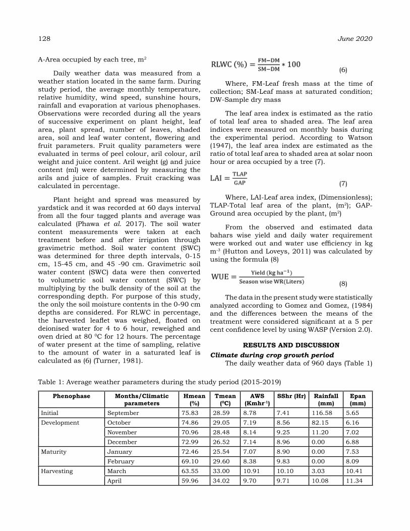
128 June 2020

A-Area occupied by each tree, m2

Daily weather data was measured from a weather station located in the same farm. During study period, the average monthly temperature, relative humidity, wind speed, sunshine hours, rainfall and evaporation at various phenophases. Observations were recorded during all the years of successive experiment on plant height, leaf area, plant spread, number of leaves, shaded area, soil and leaf water content, flowering and fruit parameters. Fruit quality parameters were evaluated in terms of peel colour, aril colour, aril weight and juice content. Aril weight (g) and juice content (ml) were determined by measuring the arils and juice of samples. Fruit cracking was calculated in percentage.

Plant height and spread was measured by yardstick and it was recorded at 60 days interval from all the four tagged plants and average was calculated (Phawa et al. 2017). The soil water content measurements were taken at each treatment before and after irrigation through gravimetric method. Soil water content (SWC) was determined for three depth intervals, 0-15 cm, 15-45 cm, and 45 -90 cm. Gravimetric soil water content (SWC) data were then converted to volumetric soil water content (SWC) by multiplying by the bulk density of the soil at the corresponding depth. For purpose of this study, the only the soil moisture contents in the 0-90 cm depths are considered. For RLWC in percentage, the harvested leaflet was weighed, floated on deionised water for 4 to 6 hour, reweighed and oven dried at 80 0C for 12 hours. The percentage of water present at the time of sampling, relative to the amount of water in a saturated leaf is calculated as (6) (Turner, 1981).

(6)

Where, FM-Leaf fresh mass at the time of collection; SM-Leaf mass at saturated condition; DW-Sample dry mass

The leaf area index is estimated as the ratio of total leaf area to shaded area. The leaf area indices were measured on monthly basis during the experimental period. According to Watson (1947), the leaf area index are estimated as the ratio of total leaf area to shaded area at solar noon hour or area occupied by a tree (7).

(7)

Where, LAI-Leaf area index, (Dimensionless); TLAP-Total leaf area of the plant, (m2); GAP-Ground area occupied by the plant, (m2)

From the observed and estimated data bahars wise yield and daily water requirement were worked out and water use efficiency in kg m-3 (Hutton and Loveys, 2011) was calculated by using the formula (8)

(8)

The data in the present study were statistically analyzed according to Gomez and Gomez, (1984) and the differences between the means of the treatment were considered significant at a 5 per cent confidence level by using WASP (Version 2.0).

reSuLtS aNd dISCuSSIoNClimate during crop growth period

The daily weather data of 960 days (Table 1)

Table 1: Average weather parameters during the study period (2015-2019)

Phenophase Months/Climatic parameters

hmean (%)

tmean (0C)

aWS (Kmhr-1)

SShr (hr) rainfall (mm)

epan (mm)

Initial September 75.83 28.59 8.78 7.41 116.58 5.65Development October 74.86 29.05 7.19 8.56 82.15 6.16

November 70.96 28.48 8.14 9.25 11.20 7.02December 72.99 26.52 7.14 8.96 0.00 6.88

Maturity January 72.46 25.54 7.07 8.90 0.00 7.53February 69.10 29.60 8.38 9.83 0.00 8.09

Harvesting March 63.55 33.00 10.91 10.10 3.03 10.41April 59.96 34.02 9.70 9.71 10.08 11.34

at an experimental site of ICAR-NRCP, Solapur covering the period from September, 2015 to April, 2019 was analyzed for calculating reference crop evapotranspiration (ETr). The average monthly ETr and rainfall in mm are shown in Fig. 1. It is revealed that the trend of the estimated ETr and rainfall values over the days are in different due to variation in climatic parameters. From Fig. 1shows that rainfall distribution was higher, estimated ETr and temperature is less in the month of September to November (i.e.new leaf initiation) and it’s useful for flowers initiation. During crop development period (i.e. December- January) no rainfall and low temperature and it’s useful for fruit setting and disease occurred very less.However, rainfall amount were low and temperature and estimated ETris high in the month of February to April (i.e. maturity and harvesting) and also useful for colour development of fruit and aril. The average hasta bahars rainfall was 223.03 mm.

Fig. 1: Average monthly temp (0C), ETr and rainfall values in mm

Reference crop evapotranspiration (ETr, mm) and rainfall (R, mm)

The average monthly reference crop evapotranspiration (ETr) estimated by Penman-Monteith Method is presented in Fig. 1. It is revealed that ETr is the highest in March-April (10-18 SW) and lowest in the month of September-November (36-44 SW) during the study period. During the study period, the average ETr and rainfall at various phenophases of new leaf initiation, development, maturity and harvesting periods are 123.57, 392.30, 325.30, 441.37 and 132.85, 102.13, 0.00, 9.15 mm, respectively. The average reference crop evapotranspiration (ETr, mm) and rainfall (R, mm) was 1282.44 and 223.04mm with a minimum and maximum of 4.12 and 8.01mm day-1 during September and April, respectively.

Crop coefficient (Kc) and wetted area (WA)

The crop coefficient values for different phenological stages of pomegranate are given in Fig 2. On an average crop coefficient (Kc) values varied in the ranged 0.25-1.10 and 0.20-0.65 for 3-6 yearold pomegranate treesduring new leaf initiation, development, maturity and harvesting period. It may be seen that Kc values are low during the initial stage of growth and gradually increasing trend during the development phase. However, the Kc values of 3-6 year’s old pomegranate tree showed the four distinct phases of Kc. Initially, the Kcvalues increased from 0.25 to 0.75 for 3rd, 0.30 to 0.90 for 4th, 0.40 to 1.0 for 5th and 0.45 to 1.10 for 6th year old pomegranate tree. The Kc values are then almost constant from crop maturity 0.70, 0.80 and 0.95. The trend observed in Kc values decline gradually during harvesting stage. During harvesting period, crop coefficient decreased from 0.75 to 0.35, 0.90 to 0.50, 1.0 to 0.55 and 1.10 to 0.65 for 3-6 year’s plant due to leaf drop, less amount of irrigation, removing of water sprout and harvesting of fruit. Higher the crop coefficient, it means the weather demand for water is high during development and maturity when the crop is in a good state of health. The trend observed in Kc values of pomegranate during different phases of growth were compared for those given by Bhantana and Lazarovitch, 2010; Gorantiwar et al. 2011 agreed fairly well and phenophase wise wetted area was computed and it showed that, average wetted area was found at various phenophase wise (i.e. new leaf initiation to harvesting) ranged from 0.20 to 0.40, 0.30 to 0.50, 0.40 to 0.60 and 0.45 to 0.70 for 3-6 year old pomegranate trees.

Fig. 2: Average phenophase wise crop coefficient and wetted area values in fraction

Actual and deficitwater requirement (ETp, Lphase-1tree-1)

The actual water applied for pomegranate


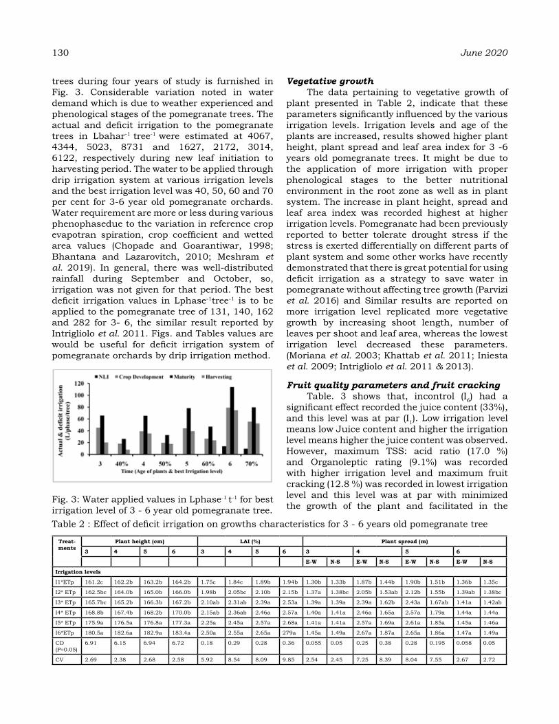
130 June 2020

trees during four years of study is furnished in Fig. 3. Considerable variation noted in water demand which is due to weather experienced and phenological stages of the pomegranate trees. The actual and deficit irrigation to the pomegranate trees in Lbahar-1 tree-1 were estimated at 4067, 4344, 5023, 8731 and 1627, 2172, 3014, 6122, respectively during new leaf initiation to harvesting period. The water to be applied through drip irrigation system at various irrigation levels and the best irrigation level was 40, 50, 60 and 70 per cent for 3-6 year old pomegranate orchards. Water requirement are more or less during various phenophasedue to the variation in reference crop evapotran spiration, crop coefficient and wetted area values (Chopade and Goarantiwar, 1998; Bhantana and Lazarovitch, 2010; Meshram et al. 2019). In general, there was well-distributed rainfall during September and October, so, irrigation was not given for that period. The best deficit irrigation values in Lphase-1tree-1 is to be applied to the pomegranate tree of 131, 140, 162 and 282 for 3- 6, the similar result reported by Intrigliolo et al. 2011. Figs. and Tables values are would be useful for deficit irrigation system of pomegranate orchards by drip irrigation method.

Fig. 3: Water applied values in Lphase-1 t-1 for best irrigation level of 3 - 6 year old pomegranate tree.

Vegetative growth The data pertaining to vegetative growth of

plant presented in Table 2, indicate that these parameters significantly influenced by the various irrigation levels. Irrigation levels and age of the plants are increased, results showed higher plant height, plant spread and leaf area index for 3 -6 years old pomegranate trees. It might be due to the application of more irrigation with proper phenological stages to the better nutritional environment in the root zone as well as in plant system. The increase in plant height, spread and leaf area index was recorded highest at higher irrigation levels. Pomegranate had been previously reported to better tolerate drought stress if the stress is exerted differentially on different parts of plant system and some other works have recently demonstrated that there is great potential for using deficit irrigation as a strategy to save water in pomegranate without affecting tree growth (Parvizi et al. 2016) and Similar results are reported on more irrigation level replicated more vegetative growth by increasing shoot length, number of leaves per shoot and leaf area, whereas the lowest irrigation level decreased these parameters. (Moriana et al. 2003; Khattab et al. 2011; Iniesta et al. 2009; Intrigliolo et al. 2011 & 2013).

Fruit quality parameters and fruit cracking Table. 3 shows that, incontrol (I6) had a

significant effect recorded the juice content (33%), and this level was at par (I1). Low irrigation level means low Juice content and higher the irrigation level means higher the juice content was observed. However, maximum TSS: acid ratio (17.0 %) and Organoleptic rating (9.1%) was recorded with higher irrigation level and maximum fruit cracking (12.8 %) was recorded in lowest irrigation level and this level was at par with minimized the growth of the plant and facilitated in the

Table 2 : Effect of deficit irrigation on growths characteristics for 3 - 6 years old pomegranate tree

treat-ments

Plant height (cm) LaI (%) Plant spread (m)

3 4 5 6 3 4 5 6 3 4 5 6

e-W N-S e-W N-S e-W N-S e-W N-S

Irrigation levels

I1*ETp 161.2c 162.2b 163.2b 164.2b 1.75c 1.84c 1.89b 1.94b 1.30b 1.33b 1.87b 1.44b 1.90b 1.51b 1.36b 1.35c

I2* ETp 162.5bc 164.0b 165.0b 166.0b 1.98b 2.05bc 2.10b 2.15b 1.37a 1.38bc 2.05b 1.53ab 2.12b 1.55b 1.39ab 1.38bc

I3* ETp 165.7bc 165.2b 166.3b 167.2b 2.10ab 2.31ab 2.39a 2.53a 1.39a 1.39a 2.39a 1.62b 2.43a 1.67ab 1.41a 1.42ab

I4* ETp 168.8b 167.4b 168.2b 170.0b 2.15ab 2.36ab 2.46a 2.57a 1.40a 1.41a 2.46a 1.65a 2.57a 1.79a 1.44a 1.44a

I5* ETp 175.9a 176.5a 176.8a 177.3a 2.25a 2.45a 2.57a 2.68a 1.41a 1.41a 2.57a 1.69a 2.61a 1.85a 1.45a 1.46a

I6*ETp 180.5a 182.6a 182.9a 183.4a 2.50a 2.55a 2.65a 279a 1.45a 1.49a 2.67a 1.87a 2.65a 1.86a 1.47a 1.49a

CD (P=0.05)

6.91 6.15 6.94 6.72 0.18 0.29 0.28 0.36 0.055 0.05 0.25 0.38 0.28 0.195 0.058 0.05

CV 2.69 2.38 2.68 2.58 5.92 8.54 8.09 9.85 2.54 2.45 7.25 8.39 8.04 7.55 2.67 2.72

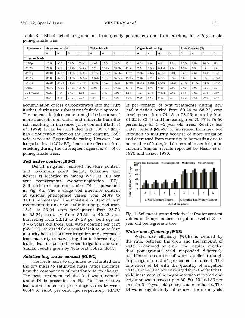
accumulation of less carbohydrates into the fruit further, during the subsequent fruit development. The increase in juice content might be because of more absorption of water and minerals from the soil resulting in increased juice content (Nath et al., 1999). It can be concluded that, 100 %* (ETp) has a noticeable effect on the juice content, TSS: acid ratio and Organoleptic rating. However, low irrigation level (20%*ETp) had more effect on fruit cracking during the subsequent ages (i.e. 3 – 6) of pomegranate trees.

Soil water content (SWC) Deficit irrigation reduced moisture content

and maximum plant height, branches and flowers is recorded in having WSV at 100 per cent pomegranate evapotranspiration (ETp). Soil moisture content under DI is presented in Fig. 4a. The average soil moisture content at various phenophase varies from 24.49 to 31.00 percentages. The moisture content of best treatments during new leaf initiation period from 15.24 to 23.24, crop development from 25.22 to 33.24; maturity from 35.36 to 40.22 and harvesting from 22.12 to 27.28 per cent age for 3 – 6 years old trees. Soil water content per cent (SWC, %) increased from new leaf initiation to fruit maturity because of more irrigation and decreased from maturity to harvesting due to harvesting of fruits, leaf drops and lesser irrigation amount. Similar results given by Noar and Cohen, 2003.

Relative leaf water content (RLWC) The fresh mass to dry mass to saturated and

the dry mass to saturated mass ratios indicates how the components of contribute to its change. The best treatment relative leaf water content under DI is presented in Fig. 4b. The relative leaf water content in percentage varies between 60.44 to 88.50 per cent age, respectively. RLWC

in per centage of best treatments during new leaf initiation period from 60.44 to 68.25, crop development from 74.15 to 78.25; maturity from 81.22 to 88.45 and harvesting from 70.77 to 76.60 percentage for 3 –6 year old trees. Relative leaf water content (RLWC, %) increased from new leaf initiation to maturity because of more irrigation and decreased from maturity to harvesting due to harvesting of fruits, leaf drops and lesser irrigation amount. Similar results reported by Hsiao et al. 1976 and Hsiao, 1990.

Fig. 4: Soil moisture and relative leaf water content values in % age for best irrigation level of 3 - 6 year old pomegranate tree.

Water use efficiency (WUE) Water use efficiency (WUE) is defined by

the ratio between the crop and the amount of water consumed by crop. The results revealed that pomegranate yield responded differently to different quantities of water applied through drip irrigation and it’s presented in Table 4. The influences of DI with the quantity of irrigation water applied and are envisaged form the fact that, yield increment of pomegranate was recorded and irrigation water saved up to 60, 50, 40 and 30 per cent for 3 - 6 year old pomegranate orchards. The DI water significantly influenced the mean yield

Table 3 : Effect deficit irrigation on fruit quality parameters and fruit cracking for 3-6 yearsold pomegranate tree

treatments Juice content (%) tSS:acid ratio organoleptic rating Fruit Cracking (%)

3 4 5 6 3 4 5 6 3 4 5 6 3 4 5 6

Irrigation levels

I1*ETp 28.5e 30.0c 31.5c 33.0d 14.0d 15.0c 14.7c 15.2c 6.2d 6.8c 8.1d 7.2e 12.8a 9.5a 10.2a 12.4a

I2* ETp 29.0e 30.2c 32.7b 34.5cd 15.2c 15.2bc 15.5bc 15.5c 7.2c 7.5bc 8.4cd 7.6e 10.2a 8.5b 8.6b 9.7a

I3* ETp 30.0d 32.0b 34.5b 35.2bc 15.7bc 16.5ab 15.5bc 15.7c 7.8bc 7.6bc 8.6bc 8.0d 3.3d 2.5d 4.3d 6.2d

I4* ETp 31.0c 32.5b 34.5b 36.2ab 16.5ab 16.5ab 16.5ab 16.2bc 7.9bc 7.7b 8.8ab 8.3bc 6.0c 4.6c 5.7cd 6.6cd

I5* ETp 32.2b 34.0a 34.7b 37.7b 16.7bc 16.7a 16.6a 17.0ab 8.6ab 8.2ab 8.9ab 8.6ab 7.7bc 5.1bc 6.5bc 8.5bc

I6*ETp 33.7a 35.0a 37.2a 38.0a 17.0a 17.5a 17.0a 17.5a 9.1a 8.7a 9.1a 9.0a 8.0b 7.0c 7.2c 8.7c

CD (P=0.05) 0.95 1.34 2.62 1.62 1.21 1.32 1.02 1.13 1.07 0.78 0.303 0.45 1.84 1.60 2.11 2.80

CV 2.05 2.76 5.10 2.98 5.14 5.42 4.20 4.63 9.18 6.65 2.33 3.75 15.53 17.1 20.0 21.3


132 June 2020

which is evident from the fact that, the mean yield in absolute quantities was considerably reduced in comparison to other irrigation level. The best irrigation level recorded the mean yield are 7.30, 13.2, 14.6 and 18.9 kg tree-1 at 40, 50, 60 and 70 per cent irrigation levels for 3 –6 year old pomegranate trees. Similarly, in irrigation levels of drip irrigation had a significant effect on the water use efficiency. Irrigation level at 40, 50, 60 and 70 per cent recorded better numbers of fruit, weight of fruits and yield because drip irrigation and needful irrigation provided a consistent moisture regime in the soil due to which root remains active throughout the phenophase resulting in optimum availability of moisture and proper translocation of food materials which accelerated the fruit growth and development of quality characters in the fruits. The table clearly indicates that different irrigation level had a significant effect on water use efficiency of pomegranate. As regards best deficit irrigation level, maximum water use efficiency was 4.3, 5.7, 5.2, 3.7 kgm-3 at 40, 50, 60 and 70 per cent for 3 -6 year old pomegranate orchards in Hasta bahar. Earlier, Smitle et al. 1994 and Abd E1-Samad, 2005 mentioned that increased water use efficiency and fruit yield due to a reduction in crop evapotranspiration and deep percolation, leading to increased yields and water use efficiency and similar results demonstrated that the improved peel color of apple fruit under deficit irrigation was the results of changes in canopy structure and increased yield and water use efficiency, while TSS in the fruits may be due to translocation of assimilate from the leaves to fruits (Wang et al. 2012; Yan et al. 2012; Francaviglia et al. 2013; Consoli et al. 2017).

CoNCLuSIoNA significant effect of DI irrigation on plant

physiology in pomegranate plants was revealed. As for as fruit quality is concerned, data indicated a positive impact of DI irrigation on reducing fruit cracking provided that the amount of irrigation water applied could replace the evapotranspiration losses. The DI impacts both the pomegranate water productivity and fruit quality.

The reference crop evapotranspiration, crop coefficient, wetted area and water requirement values varied in the range from 4.12 to 8.01 mm, 0.25 to 1.10, 0.40 to 0.60, 10.5 to 37.5 L d-1 t-1 during new leaf initiation, development, maturity and harvesting phase, respectively. On an average pomegranate fruit crop consumed

Tabl

e 4

: Effe

ct o

f defi

cit

irri

gati

on o

n y

ield

att

ribu

tes

and

wat

er u

se e

ffici

ency

for

3 -

6 ye

ars

old

pom

egra

nat

e tr

ees

tre

atm

ents

Nos

. of

frui

t pe

r tr

. (N

os.)

av.

Fru

it W

eigh

t (g

ms)

Y

ield

(kgt

ree-1

) W

u (m

3 )

Wu

e (K

gm-3)

34

56

34

56

34

56

34

56

34

56

I1*E

Tp14

.7e

25.4

c40

.5c

32.2

b23

9.5c

313.

3c26

1.5c

265.

5c3.

5f8.

08c

10.6

c8.

7b0.

781.

730

1.94

43.

383.

5c4.

6b5.

4a2.

6b

I2*

ETp

19.2

d26

.2c

42.2

b38

.0b

281.

5b28

9.2c

277.

7bc

271.

7bc

5.4e

7.5c

11.7

bc10

.2b

1.18

11.

827

2.43

14.

224.

6ab

4.2b

4.8a

2.5b

I3*

ETp

24.5

c42

.2b

47.5

a60

.5a

300.

0ab

310.

5b30

7.5a

b31

3.7a

7.3d

13.2

b14

.6a

18.9

a1.

574

2.28

42.

917

5.07

4.6a

5.7a

5.2a

3.7a

I4*

ETp

30.7

b41

.0b

42.7

c52

.2a

299.

0ab

302.

7b30

5.0a

b30

1.5a

b7.

2c12

.4b

12.9

ab15

.7a

1.96

82.

740

3.40

35.

914.

6a4.

5a3.

9b2.

6b

I5*

ETp

33.7

b43

.7b

45.5

b52

.0a

301.

7ab

299.

2a30

2.7a

b31

0.5a

10.2

b13

.0a

137a

16.1

a2.

362

3.19

73.

889

6.75

4.2a

b4.

0b3.

5c2.

3b

I6*E

Tp36

.5a

54.0

a47

.5a

57.7

a31

7.5a

336.

2a30

2.5a

311.

7a11

.6a

18.1

a14

.2a

18.0

a2.

985

4.23

54.

861

8.44

3.9b

c4.

2b2.

9c2.

2b

CD

(P=0

.05)

3.

195.

46.

7810

.85.

037.

096.

097.

330.

971.

91.

82.

5--

----

--0.

698

0.73

50.

639

0.68

6

CV

7.90

9.27

9.04

14.7

21.9

722

.10

29.5

32.7

08.

9110

.39.

3315

.8--

----

--10

.81

10.6

79.

9317

.10

(Not

e :

I 1-20

, I 2-

30,

I 3-40

, I 4-

50,

I 5-60

& I 6

-100

%*E

T p fo

r 3rd

; I 1-

30,

I 2-40

, I3

-50,

I4-

60,

I 5-70

& I 6

-100

%*E

T p fo

r 4th

; I1 -

40,

I2 -50

, I3 -

60,

I4 -70

I5-

80 &

I 6 -1

00%

*ET p

for

5th a

nd

I 1-50

, I2-

60, I

3-70

, I4-

80, I

5-90

& I 6

-100

%*E

T p fo

r 6th

)

about 1574; 2284;2917and 5073 Lbahar-1 t-1 at 40, 50, 60 and 70 per cent of pomegranate evapotranspiration (ETp). Water use efficiency was 4.30, 5.70, 5.20 and 3.70kg m-3 for 3 - 6 year old pomegranate orchards at 40, 50, 60 and 70 per cent of pomegranate evapotranspiration (ETp) is the best irrigation level. Water use efficiency does not depend only on the total amount of water consumed by the crop but also on its distribution during the various growth stages of the crop.

Water conserved technologies ensure increased crop yield, high water use efficiency, reduced water and energy consumption. In conclusion: 40, 50, 60 and 70 per cent of pomegranate evapotranspiration (ETp) is recommended, applicable water saving strategy when water resources are limited in order to increase WUE while other physiological and growth parameters are maintained at an acceptable level.

aCKNoWLedgMeNtSThe authors express their appreciation to

ICAR-NRC on pomegranate Research Institute, Solapur and Indian Council of Agricultural Research, New Dehli for financial support of the project. It is necessary to thanks Shri. B.S. Waghmode, Shri. Nagraj Bake and Shri. S. A. Lad for their valuable helps and supports.

reFereNCeSAbd E1 Samad, G.A. (2005). Water use, growth

and productivity of some new guava strain as affected by different irrigations regimes. Egypt J. Hort., 32:41-56.

Ahamadi, S.H., Andersen, M.N., Plauborg, F., Poulsen, R.T., Jensen, C. R., Sepaskhah, A. R. and Hansen, S. (2010). Effect of irrigation strategies and soils on field grown potatoes: Yield and water productivity. Agri. Water Manag., DOI 10.116/j.agwat. 2010.07.007.

Allen, R.G., Pereira, L.S., Raes, D. and Smith, M. (1998).Crop evapotranspiration, guideline for computing crop water. FAO Irrigation and Drainage Paper 56. FAO Rome, Italy, Pp. 300.

Aseri, G.K., Jain, N., Panwar, J., Rao, A.V. and Meghwal, P.R. (2008). Bio-fertilizers improve plant growth, fruit yield, nutrition metabolism and rhizosphere enzyme activities of pomegranate (Punicagranatum L.) in India Thar Desert. Sci. Hort., 117 (2) :130-135.

Ayers, J.E., Johnsons, R.S., Phene, C.J., Trout, T.J., Clark, D.A. and Mead, R.M. (2005). Water use by drip irrigated late season Peaches. Irri. Sci., 22: 187-194.

Bhantana, P. and Lazarovitch, N. (2010).Evapotranspiration, crop coefficient and growth of two young pomegranate (PunicagranatumL.) varieties under salt stress.Agri. Water Manag., 97:715-722.

Chalmers, D.J., Mitchell, P.D. and Van Heek, L. (1981).Control of peach tree growth and productivity by regulated water sup¬ply, tree density, and summer pruning.J. American Soc. Hort. Sci., 106:307-312.

Chopade, S.O. and Gorantiwar, S.D. (1998).Effect of various methods of irrigation on growth and yield of pomegranate.Ann. plant Phys., 12:98-102.

Consoli, S., Stagno, F., Vanella, D., Boaga, J., Cassiani, G. and Roccuzzo, G. (2017). Partial root zone drying irrigation in Orange orchards: Effects on water use and crop production characteristics., 82:190-202.

Dying pomegranates and the threat to India’s new framing; available at: http:// www.indiaspend.com/cover- story/89610 (Accessed 25th May, 2018).

Fereres, E. and Soriano, M.A. (2007).Deficit irrigation for reducing agricultural water use.J. Exp. Bot., 58 (2) :147-159.

Francaviglia, D., Farina, V., Avellone, G. and Lo Bianco, R. (2013). Fruit yield and quality response of apple cavrs Gala and Fuji to partial root zone drying under Mediterranean conditions. J. Agri. Sci., 151:556-569.

Goldhamer, D.A., Viveros, M. and Salinas, M. (2006). Regulated deficit irrigation in Almonds: effects of variations in applied water and stress timing on yield and yield components. Irri. Sci., 24 (2) :101-114.

Gomez, K.A. and Gomez, A.A. (1984).Statistical Procedures for Agricultural Research. A Wiley Inter Science Publication, John Wiley and Sons, New York, 680 Pp.

Gorantiwar, S.D., Meshram, D.T. and Mittal, H.K. (2011).Water requirement of pomegranate for Ahmednagar district part of Maharashtra.J. Agrometorol., 13 (2) :123-127.

Hsiao, T.C., Acevedo, E., Fereres, E. and Henderson, D.W. (1976). Stress metabolism. Water tress, growth and osmotic adjustment.


134 June 2020

Philos T Roy Soc B. 273:479-500. Hsiao, T. (1990). Measurement of plant water

status.In:steward B, Nielsen D, editos. Irrigation of Agriculture Crops. Agronomy Monographs No. 30. Madison, WI USA”ASA.243-279.

Holland, D. and Bar-Ya’akov, I. (2008). The pomegranate: New interest in an ancient fruit, Chron. Horti., 48:12-15.

Holland, D., Hatib, K. and Bar-Ya’akov, I., (2009). Pomegranate: botany, horticulture, breeding. In: Janick J (Ed) Horti. Reviews, John Wiley and Sons, New Jersey. 35:127-191.

Holzapfel, E.A., Marino, M.A., Valenzuela, A. and Diaz, F. (1988).Comparison of infiltration measuring methods for surface irrigation.J. Irri. and Drai. Engi., 114 (1) 130-142.

Hutton, R.L. and Loveys, B.R. (2011).A partial root zone drying irrigation strategy for Citrus effects on water use efficiency and fruit characteristics.Agri. Water Manage., 98:1485-1496.

Iniesta, F., Testi, L., Orgaz, F. and Villalobos, F.J. (2009). The effects of regulated and continuous deficit irrigation on the water use, growth and yield of olive trees. Eur. J. Agron., 30: 258-265.

Intrigliolo, D.S., Nicolas, E., Bonet, L., Ferrer, P., Alarcon, J.J. and Bartual, J. (2011). Water relation of field grown pomegranate trees (Punicagranatum L.) under different drip irrigation regimes. Agri. Water Manag., 98 (4) :691-696.

Intrigliolo, D.S., Bonet, L., Nortes, P.A., Puerto, H., Nicolas, E. and Bartual, J. (2013). Pomegranate trees performance under sustained and regulated deficit irrigation. Irri. Sci., 31:959-970.

Kaulgud, S.N. (2001). Pomegranate.In:Chadha, K.L. (ed.), Hand book of Horticulture, pp:397-307. ICAR, New Dehli.

Khattab, M.M., Shaban, A.E., El-Shrief, A.H. and El-Deen Mohamed, A.S. (2011). Growth and productivity of pomegranate trees under different irrigation levels I: vegetative growth and fruiting. J. Hort. Sci. Ornamental plants., 3:194-198.

Melgarejo, P., Martinez-Valero, R., Guilamon, J.M., Miro, M. and Amoros, A. (1997). Phenological stages of the pomegranate tree

(Punicagranatum L.) Ann. App. Biol. 130: 135-140.

Meshram, D.T., Gorantiwar, S.D., Mittal, H.K., Singh, N.V. and Lohkare, A.S. (2012). Water Requirement of Pomegranate (Punicagranatum L.) plants upto five year age. J. Appl. Hort., 14 (1) : 47-51.

Meshram, D.T., Gorantiwar, S.D., Singh, N.V. and Dhinesh Babu. (2019). Response of micro-irrigation systems on growth, yield and WUE of pomegranate (Punicagranatum L.) in Semi-Arid Regions of India.Sci. Hort., 246:686-692.

Miguel Costa, J., Ortuno, M.F., and Manuela Chaves, M. (2007). Deficit Irrigation as a Strategy to Save Water: Physiology and Potential Application to Horticulture. J. Integr. Plant Bio., 49 (10) : 1421-1443.

Moriana, A., Orgaz, F., Pastor, M. and Fereres, E. (2003). Yield responses of a mature olive orchard to water deficits. J.Amer. Soc. Hort. Sci., 128: 425–431.

National Horticulture Board, (2017). Available at: http://nhb.gov.in / statistics/area-production-statistics.html/ (accessed 20th October, 2018).

Nath, V., Singh, R. S., Sharma, B. D. and Pareek, O. P. (1999).Shuskhabagwanievaimjalprabandh.Phal Phool., 22: 11-14.

Naor, A. and Cohen, S. (2003). Sensitivity and variability of maximum trunk shrinkage, midday steam water potential and transpiration rate in response to withholding irrigation from field grown apple trees. Hort.Sci., 38:547-551.

Pal, R.K., DhineshBabu, Singh, N.V., Ashis Maityand Gaikwad, N. (2014).Pomegranate research in India-status and future challenges.Progressive Hort., 46 (2) : 184-201.

Parvizi, H., Sepaskhah, A.R. and Ahmadi, S.H. (2016). Physiological and growth responses of pomegranate tree (Punicagranatum (L.) cv. Rabab) under partial root zone drying and deficit irrigation regimes. Agri. Water Manag., 163:146-158.

Phawa, T., Prasad, V.M. and Rajwade, V.B. (2017). Effect of plant growth regulators on growth and flowering of pomegranate (Punicagranatum L.) Cv. Kandhari in Allahabad Agro climatic condition. Int. J. Curr. Microbiol. App. Sci., 6 (8) :116-121.

Smitle, D.A., Dickens, W. and Stansell, J.R. (1994). Irrigation regimes affect yield and water use by Bell Pepper. J. American Soc. Hort. Sci., 119:936.

Stover, E. and Mercure, E.W. (2007). The Pomegranate: A new look at the fruit of paradise. Hort. Sci. 1088-1092.

Turner, N.C. (1981). Techniques and experimental approaches for the measurement of plant water status. Plant Soil. 58: 339–366.

Wang, S., Liang, D., Li, C., Hao, Y., Ma, F. and Shu, H. (2012). Influence of drought stress on the cellular ultra structure and antioxidant system in leaves of drought-tolerant and drought-sensitive apple root stocks. Plant Physiol. Biochem., 51:81-89.

Watson, D.J. (1947). Comparative physiological studies in the growth of field crops. I: variation in net assimilation rate and leaf area between species and varieties, and within and between years. Ann. Bot., 11: 41-76.

Yang, L., Qu, H., Zhang, Y. and Li, F. (2012). Effects of partial root zone drying on physiology, fruit yield and quality and water use efficiency of tomato under different calcium levels. Agri. Water Manage., 104:89-94.

Zhang, H. and Wang, D. (2013). Management of postharvest deficit irrigation of peach trees using infrared canopy temperature. Vad.Zon. J., Doi:10.2136/vzj2012.0093.


Farmers’ Preparedness to manage grape diseases through agromet advisories based on Weather based Forecast Models

raghaveNdra aCharI1, h. veNKateSh2 aNd hIreMath, J.r.3

1Horticultural Research and Extension Centre, Vijayapura (Tidagundi), UHS Bagalkot2 Director of Extension, UAS Dharwad

2 Regional Agricultural Research Station, Vijayapura, UAS Dharwad

aBStraCtGrape requires more fungicides for the management diseases, which necessitated disease forecasting systems. The Per cent disease severity (PDI) of anthracnose, downy mildew (DMD) and powdery mildew (PMD) diseases were recorded during 2013 to 2016 and subjected to correlation analysis using lead time concept with weather parameters of both current week (LT0) and one week ahead (LT1). The diurnal variation of RH for anthracnose; and maximum temperature at LT1, and minimum temperature and temperature range at LT0 are important for forecasting PMD. The farmers spray details (2014, 2015 and 2016) were compared with corresponding weather to identify the favourable weather conditions for each disease. For incidence of anthracnose, morning (80%) and afternoon RH (35-50%), for PMD, maximum temperature of > 29°C with >6 hrs sunshine duration and for DMD, maximum temperature of around 26°C and <6 hrs sunshine duration were important. When these criteria were tested during 2017, five out of eight weeks for PMD and all seven weeks for DMD were successfully forecasted. Lead time concept using medium range weather forecasts of IMD, Agromet advisories are being provided to farmers for timely management of grape diseases.

Keywords: Lead time, correlation, Agromet

INtroduCtIoN

Weather has a highly dominant influence on incidence of most of the plant diseases and insect pests. Integrated Pest Management (IPM) methods are important under the plant protection umbrella. But, they do not generally include the weather factor. Adopting an approach of selecting plant protection practices based on weather parameters adds logical decision making value to IPM strategies. The importance of disease forecasting/forewarning for farmers is all about impending weather and its possible effect on incidence of pests and diseases leading to decision making about time of implementation of management practices and selection of preventive measures over curative pesticides. By adopting the measures pro-actively, farmers can save the crop and also reduce possible adverse impact of pesticides on environment. Disease forecast/prediction is about expecting the occurrence of disease by a few days or weeks in advance, whereas forewarning is much more specific over forecast/predict by providing warning along with set of advisories to help the farmer for decision making. For this purpose, ‘Lead time concept’ is one such approach from which we can know the incidence

of disease in advance by some time, which is called as ‘Lead time’. The lead time may be couple of days to a week. This is basically ‘predicting the effect by monitoring the cause’. Pre-requisites for forewarning include knowing climate information, crop stage, duration and stage of diseases/pests.

MaterIaL aNd MethodS:The disease severity incidence data recorded

as per cent disease index (PDI) of downy mildew, anthracnose and powdery mildew diseases on grape variety Thompson Seedless were collected at weekly interval at HREC, Vijayapur (Tidagundi) on selected untreated grapevines earmarked for various chemical testing trials from 2012-13 to 2015-16. The data on incidence of the disease were recorded by following common disease rating scale for all diseases as detailed below. The per cent disease index (PDI) was calculated from the disease ratings as detailed below.

Disease rating scale followed for recording the incidence of downy mildew and anthracnose disease of grapes.


disease rat-ing/ grade

Per cent area covered/ infection

0 No disease/Infection1 1-10 % area covered/infection2 10.1-15% area covered/infection3 15.1-25% area covered/infection4 25.1-50 % area covered/infection5 >50% area covered/infection

Per cent disease index (PDI) was calculated by using the formula proposed by Wheeler (1969).

The data of the grape diseases observed are presented graphically, and the relationship between disease PDI and corresponding weather variables of both current week and previous, i.e., Zero weeks lead time (LT0) and one week lead time (LT1), respectively was assessed by correlation analysis. The daily meteorological data from 10 days after pruning till the harvest of crop was used for the present analysis. The meteorological parameters, namely, Maximum temperature (Tmax), Minimum temperature (Tmin), TR- Diurnal range of temperature (TR), Relative Humidity (%) at 0700 hrs LMT (RH1), Relative Humidity (%) at 1400 hrs LMT (RH2), Diurnal range of relative humidity (RHR) and Bright Sunshine Duration (hours) (BSS) at zero (LT0) and one week lead time (LT1) were considered as causal variables for correlation studies with the incidence of disease which was considered as the effect.

Another approach was adopted in farmers’ fields. In commercial crops like grape, farmers never have any plot without taking any control measures. Hence, it was decided to assess the role of weather variables for the periods in which farmers adopted control measures for the management of various pests and diseases. For this purpose we identified two farmers in a nearby village Jumanal, which is less than five kilo meters from Regional Agricultural Research Station (RARS), Vijayapura, and therefore the weather data collected at RARS was extended as representative for Jumanal village also. Since, normally disease control measures are not adopted in pathological trials, and grape farmers always take up control measures, this procedure was adopted on trial basis, and without affecting

the spray schedule of the farmers. The time of pruning was different in the two farmers’ fields, and hence the respective grape vines got different growing environments.

The spray schedule implemented by the contact farmers in Jumanal village were collected on real time basis, and the weather conditions that prevailed between two sprays were used to identify the prevailing weather conditions for taking up spray for individual pest/disease. The data for all such intervals were assessed and the information is presented in the form of tables. The data were collected for four years, among which the pest and disease problem was most during 2014, and the data of the year 2014 were considered as congenial weather conditions for respective pests and diseases.

reSuLtS aNd dISCuSSIoN:Year wise temporal profiles of incidence of

the three diseases are presented in Fig. 1. It is noticed from the figure that the diseases were noticed during 50th Standard Meteorological Week (SMW) to 10th SMW in the year 2012-13. While anthracnose and powdery mildew decreased, downy mildew showed an increasing mode during the overall study period. The diseases were noticed during the period from 5th to 15th standard weeks in the year 2013-14. The progress trend of diseases was similar to that noticed in 2012-13. In the year 2014-15, the diseases were observed between 49th standard week and 7th standard week. All diseases showed an ascending mode, but with different slopes. In the cropping year 2015-16, only data of two diseases were available for the period from 49th to 7th standard week. Both powdery mildew and anthracnose showed ascending mode in this year also. These variations are ascribed as due to interaction between time of pruning as well as prevailing weather during critical period of cropping.

In Fig. 2, pooled data of all the four years are presented for individual grape diseases viz., anthracnose, powdery mildew and downy mildew. The figure provides interesting features of the three important diseases of grapes observed during the study period.

Vol. 22, Special Issue ACHARI et al. 137

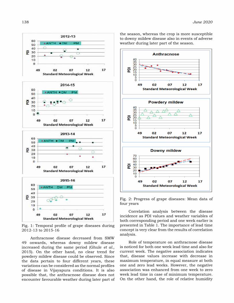
138 June 2020

Fig. 1: Temporal profile of grape diseases during 2012-13 to 2015-16

Anthracnose disease decreased from SMW 49 onwards, whereas downy mildew disease increased during the same period (Ghule et al., 2015). On the other hand, no clear trend for powdery mildew disease could be observed. Since the data pertain to four different years, these variations can be considered as the normal profiles of disease in Vijayapura conditions. It is also possible that, the anthracnose disease does not encounter favourable weather during later part of

the season, whereas the crop is more susceptible to downy mildew disease also in events of adverse weather during later part of the season.

Fig. 2: Progress of grape diseases: Mean data of four years

Correlation analysis between the disease incidence as PDI values and weather variables of both corresponding period and one week earlier is presented in Table 1. The importance of lead time concept is very clear from the results of correlation analysis.

Role of temperature on anthracnose disease is noticed for both one week lead time and also for current week. The negative association indicates that, disease values increase with decrease in maximum temperature, in equal measure at both one and zero lead weeks. However, the negative association was enhanced from one week to zero week lead time in case of minimum temperature. On the other hand, the role of relative humidity

was diminished from one week lead time to zero week lead time. Thus, instead of in combination at the same time, we found that the importance of various parameters were changing progressively as the disease approaches. Further, on operational terms, for forecasting anthracnose disease one week ahead, maximum temperature, morning relative humidity and afternoon humidity need to be considered, which can be used for raising the alerts to support the decision making regarding spray to be taken (preparedness for spray schedule). On the other hand, minimum temperature in the current week has to be taken as guide in advising for implementation of the spray schedule for anthracnose disease.

In case of both downy mildew and powdery mildew diseases, the values of correlation coefficient were not very high. Yet, for powdery mildew disease, thermal response was noticed to be significant. Maximum temperature was seen as the main parameter which has to be considered for forecast at one week lead time for the purpose of preparedness, and minimum temperature and/or temperature range at current week for actual implementation of management practices (Carroll et al., 2003). In case of downy mildew, the highest negative association, though non-significant, was with sunshine hours at Zero weeks lead time, i.e., the current week. It is identified as the only critical parameter.

Analysis of weather in relation to spray

schedule in farmers’ fields

Details of selected farmers, their farm location, area of crop along with the date of pruning are given in Table 2.

Among the five years data from 2014 to 2017, the disease incidence was diverse and damaging during 2014. So, we have considered the weather during that year as check, and the weather during other years were compared with those in 2014. The congenial weather conditions so identified are presented in Table 3.

It was noticed that sunshine duration of less than six hours as the criterion for downy mildew disease enhancement. This is supported by the correlation analysis from experimental data. These inferences were tested for other years, and the results are given below,

2015-16:It was noticed during 2014 that maximum

temperature of 29 °C to 32 °C and minimum temperature of 14 °C to 19 °C were the common temperature conditions that were experienced when powdery mildew or downy mildew diseases prevailed. During the year 2015-16, these situations were noticed between SMW 46- 49 and SMW 52 - 03 (subsequent year).

Downy mildew disease prevailed during 2014 when the maximum temperature of 26 °C to 29 °C was experienced, which never prevailed

Table 1: Correlation analysis between weather variables and incidence of grape diseases

disease Lead time (Weeks) tmax tmin tr RH1 RH2 RHR BSS

Anthracnose1 -0.81 -0.68 -0.02 0.86 0.81 0.70 -0.520 -0.79 -0.82 0.41 0.50 0.20 0.62 -0.11

Downy mildew1 -0.19 -0.33 0.25 0.36 0.22 0.38 -0.100 -0.15 -0.02 -0.21 0.42 0.25 0.41 -0.55

Powdery mildew1 0.34 0.29 0.01 -0.10 -0.15 -0.01 -0.260 0.12 -0.34 0.56 0.20 -0.03 0.33 0.30

Where Tmax- Maximum temperature (°C) ; Tmin- Minimum temperature (°C) ; TR- Diurnal temperature range (°C) ; RH1- Morning Relative Humidity (%) ; RH2- Afternoon Relative Humidity (%) ; RHR-Diurnal range of Relative Humidity (%) ; BSS-Bright Sunshine duration (hours)

Table 2 : Details of Grape farmers’ plots selected in Jumanal.

Sl.No. Farmer’s name Mobile No. area (acres) variety Lat. & Long. Pruning 01. Laxman G. Terdal 8277315562 5 Thompson

seedlessN 16O 45.619' E 75 O 43.398'

Earlier

02. Maliksab P. Bag-wan

9972189121 2 Thompson seedless

N 16O 45.795'E 75 O 43.517’

Later by 10 to 15 days

Shortest distance of Jumanal village from Agrometeorological Observatory, RARS, Vijayapura : 5 km

Vol. 22, Special Issue ACHARI et al. 139

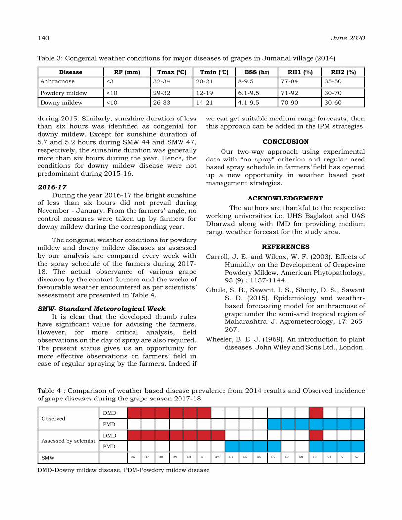
140 June 2020

during 2015. Similarly, sunshine duration of less than six hours was identified as congenial for downy mildew. Except for sunshine duration of 5.7 and 5.2 hours during SMW 44 and SMW 47, respectively, the sunshine duration was generally more than six hours during the year. Hence, the conditions for downy mildew disease were not predominant during 2015-16.

2016-17During the year 2016-17 the bright sunshine

of less than six hours did not prevail during November - January. From the farmers’ angle, no control measures were taken up by farmers for downy mildew during the corresponding year.

The congenial weather conditions for powdery mildew and downy mildew diseases as assessed by our analysis are compared every week with the spray schedule of the farmers during 2017-18. The actual observance of various grape diseases by the contact farmers and the weeks of favourable weather encountered as per scientists’ assessment are presented in Table 4.

SMW- Standard Meteorological Week It is clear that the developed thumb rules

have significant value for advising the farmers. However, for more critical analysis, field observations on the day of spray are also required. The present status gives us an opportunity for more effective observations on farmers’ field in case of regular spraying by the farmers. Indeed if

we can get suitable medium range forecasts, then this approach can be added in the IPM strategies.

CoNCLuSIoNOur two-way approach using experimental

data with “no spray” criterion and regular need based spray schedule in farmers’ field has opened up a new opportunity in weather based pest management strategies.

aCKNoWLedgeMeNt The authors are thankful to the respective

working universities i.e. UHS Baglakot and UAS Dharwad along with IMD for providing medium range weather forecast for the study area.

reFereNCeSCarroll, J. E. and Wilcox, W. F. (2003). Effects of

Humidity on the Development of Grapevine Powdery Mildew. American Phytopathology, 93 (9) : 1137-1144.

Ghule, S. B., Sawant, I. S., Shetty, D. S., Sawant S. D. (2015). Epidemiology and weather-based forecasting model for anthracnose of grape under the semi-arid tropical region of Maharashtra. J. Agrometeorology, 17: 265-267.

Wheeler, B. E. J. (1969). An introduction to plant diseases. John Wiley and Sons Ltd., London.

Table 3: Congenial weather conditions for major diseases of grapes in Jumanal village (2014)

disease rF (mm) tmax (0C) tmin (0C) BSS (hr) rh1 (%) rh2 (%) Anhracnose <3 32-34 20-21 8-9.5 77-84 35-50

Powdery mildew <10 29-32 12-19 6.1-9.5 71-92 30-70Downy mildew <10 26-33 14-21 4.1-9.5 70-90 30-60

Table 4 : Comparison of weather based disease prevalence from 2014 results and Observed incidence of grape diseases during the grape season 2017-18

ObservedDMD

PMD

Assessed by scientistDMD

PMD

SMW 36 37 38 39 40 41 42 43 44 45 46 47 48 49 50 51 52

DMD-Downy mildew disease, PDM-Powdery mildew disease

Impact of Climatic variability on Wheat Yield in Indian Subcontinent1PaNKaJ dahIYa, 2eKta PathaK MIShra*, 2BISWaruP Mehra, 1aBhILaSh,

1SureSh, 1M.L. KhIChar aNd 1raM NIWaS.1Department of Agricultural Meteorology, CCSHAU, Hisar, Haryana

2Department of Environmental Sciences and NRM, SHUATS, Prayagraj*Corresponding author: [email protected]

aBStraCtThe impact of climate influences like temperature and rainfall variation on the wheat yield in different states of India by using regression analysis statistical method has been examined in this study. The grid data of few climatic parameters and crop data were analyzed for fourteen states of Indian subcontinent during 1950 to 2015. A key observation was that temperature and precipitation together explained wheat yield variability of three states significantly which were Rajasthan (39%), Uttar Pradesh (29%) and Madhya Pradesh (22%) respectively. These three states accounts for approximately 50% of wheat production in India together. In many states, it is observed that the climate accounted for more than 20 percent of the variation in wheat yield. Rainfall alone described a variation in around 30 percent of India’s total land. However, 50% of regional wheat production is accountable for those states. In colder Nagaland, Meghalaya and Jammu & Kashmir, the temperature-induced effects were favorable for the yield of wheat, but negative for comparatively warm areas. Rise in temperature is related to reduction in wheat yield in five major wheat producing states (UP, MP, Rajasthan, Odisha and Andhra Pradesh). To find out and underline the critical significance of climate change, our research measures may be used to improve reliable and meaningful determinations of climate vs. crop dynamics for the future.

Keywords: Wheat yield, temperature, precipitation, regression, ARIMA

INtroduCtIoN

Worldwide climate change is predicted to have an imminent and significant impression on growth, development and ultimately, crop production. The main climate changes are the shifting patterns of precipitation, surface solar radiation, increase in global temperature and the ever-increasing concentration of CO2 (Monteith, 1980). The past climate variability patterns have been well evaluated for their effect on agricultural ecosystems, but the potential effects of these changes and their predictions remain inclusive (Tao et al., 2016). It is not easy to conclude on the possible impacts of climate change on site-specific crop production due to the data deficiency at site-specific levels, particularly for climatic entities (Zhang et al., 2017). There is a certain ambiguity in the estimation of possible changes in weather conditions and their penultimate consequences, which involve a much more nuanced integrated approach (Tao and Zhang, 2013). In many parts of the world, a substantial rise in the average global temperature was reported during the 20th century, along with a prominent aberration in the rainfall (Easterling et al., 1999; IPCC, 2001; Jung et al., 2002; Fauchereau et al., 2003). As

stated by IPCC, the global mean temperature rise (1to 3 °C after 1990) would have a mixed impact, and the Indian subcontinent is no exception as regards surface temperature rise, rainfall aberrations (Pant et al., 1999; Stephenson et al., 2001), and regional rainfall variations (Kripalani et al., 2003). The influence of these variations can have devastating effects on any area’s agricultural growth, and ultimately on food health (Aggarwal, 2003). Changes in temperature and precipitation are reported regionally and globally, both in terms of spatial and temporal distribution as well as in quantitative aspects, causing a broad range of input effects as well as agricultural and related production (Wolf 2002). The causes of these drastic changes in climate and the nature of these changes have always been highly debatable problems, but in the last decade some of the inconsistencies, particularly the impacts on ecosystems, have been resolved. The key explanation for global warming is the growing concentration of greenhouse gases (CO2, N2O, CH4 and CFCs) due to anthropogenic activities (Tubiello et al., 2000). The areas in the northern hemisphere above 55°C will undergo odd but positive effects of climate change on their agricultural growth (Ewert et al., 2005). Particularly in developing


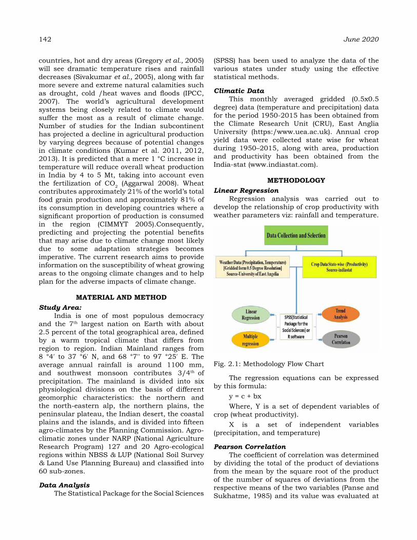
142 June 2020

countries, hot and dry areas (Gregory et al., 2005) will see dramatic temperature rises and rainfall decreases (Sivakumar et al., 2005), along with far more severe and extreme natural calamities such as drought, cold /heat waves and floods (IPCC, 2007). The world’s agricultural development systems being closely related to climate would suffer the most as a result of climate change. Number of studies for the Indian subcontinent has projected a decline in agricultural production by varying degrees because of potential changes in climate conditions (Kumar et al. 2011, 2012, 2013). It is predicted that a mere 1 °C increase in temperature will reduce overall wheat production in India by 4 to 5 Mt, taking into account even the fertilization of CO2 (Aggarwal 2008). Wheat contributes approximately 21% of the world’s total food grain production and approximately 81% of its consumption in developing countries where a significant proportion of production is consumed in the region (CIMMYT 2005).Consequently, predicting and projecting the potential benefits that may arise due to climate change most likely due to some adaptation strategies becomes imperative. The current research aims to provide information on the susceptibility of wheat growing areas to the ongoing climate changes and to help plan for the adverse impacts of climate change.

MaterIaL aNd MethodStudy Area:

India is one of most populous democracy and the 7th largest nation on Earth with about 2.5 percent of the total geographical area, defined by a warm tropical climate that differs from region to region. Indian Mainland ranges from 8 °4′ to 37 °6′ N, and 68 °7′′ to 97 °25′ E. The average annual rainfall is around 1100 mm, and southwest monsoon contributes 3/4th of precipitation. The mainland is divided into six physiological divisions on the basis of different geomorphic characteristics: the northern and the north-eastern alp, the northern plains, the peninsular plateau, the Indian desert, the coastal plains and the islands, and is divided into fifteen agro-climates by the Planning Commission. Agro-climatic zones under NARP (National Agriculture Research Program) 127 and 20 Agro-ecological regions within NBSS & LUP (National Soil Survey & Land Use Planning Bureau) and classified into 60 sub-zones.

Data AnalysisThe Statistical Package for the Social Sciences

(SPSS) has been used to analyze the data of the various states under study using the effective statistical methods.

Climatic DataThis monthly averaged gridded (0.5x0.5

degree) data (temperature and precipitation) data for the period 1950-2015 has been obtained from the Climate Research Unit (CRU), East Anglia University (https:/www.uea.ac.uk). Annual crop yield data were collected state wise for wheat during 1950–2015, along with area, production and productivity has been obtained from the India-stat (www.indiastat.com).

MethodoLogYLinear Regression

Regression analysis was carried out to develop the relationship of crop productivity with weather parameters viz: rainfall and temperature.

Fig. 2.1: Methodology Flow Chart

The regression equations can be expressed by this formula:

y = c + bxWhere, Y is a set of dependent variables of

crop (wheat productivity). X is a set of independent variables

(precipitation, and temperature)

Pearson Correlation The coefficient of correlation was determined

by dividing the total of the product of deviations from the mean by the square root of the product of the number of squares of deviations from the respective means of the two variables (Panse and Sukhatme, 1985) and its value was evaluated at

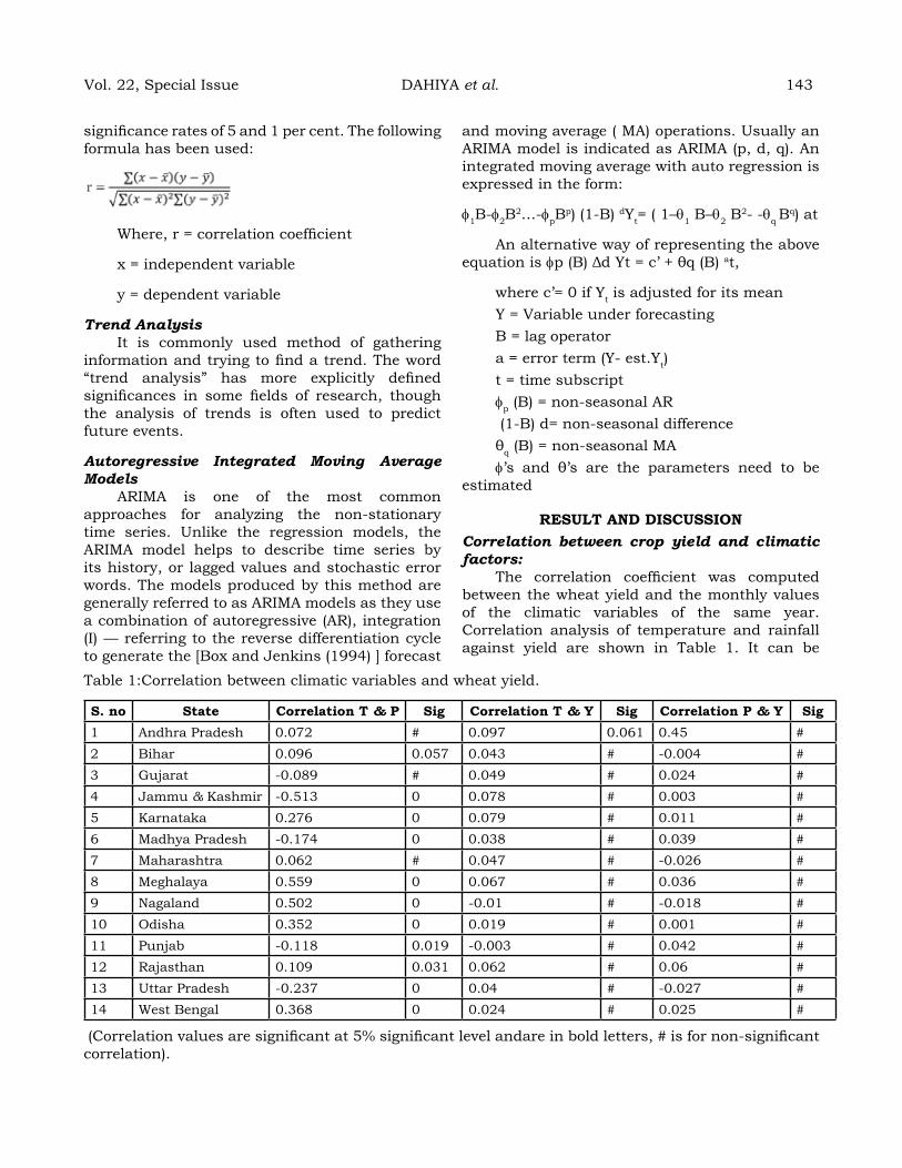
significance rates of 5 and 1 per cent. The following formula has been used:

Where, r = correlation coefficient

x = independent variable

y = dependent variable

Trend AnalysisIt is commonly used method of gathering

information and trying to find a trend. The word “trend analysis” has more explicitly defined significances in some fields of research, though the analysis of trends is often used to predict future events.

Autoregressive Integrated Moving Average Models

ARIMA is one of the most common approaches for analyzing the non-stationary time series. Unlike the regression models, the ARIMA model helps to describe time series by its history, or lagged values and stochastic error words. The models produced by this method are generally referred to as ARIMA models as they use a combination of autoregressive (AR), integration (I) — referring to the reverse differentiation cycle to generate the [Box and Jenkins (1994) ] forecast

and moving average ( MA) operations. Usually an ARIMA model is indicated as ARIMA (p, d, q). An integrated moving average with auto regression is expressed in the form:

φ1B-φ2B2…-φpB

p) (1-B) dYt= ( 1–q1 B–q2 B2- -qq B

q) at

An alternative way of representing the above equation is φp (B) Δd Yt = c’ + θq (B) at,

where c’= 0 if Yt is adjusted for its meanY = Variable under forecastingB = lag operator a = error term (Y- est.Yt) t = time subscript φp (B) = non-seasonal AR (1-B) d= non-seasonal difference θq (B) = non-seasonal MAφ’s and θ’s are the parameters need to be

estimated

reSuLt aNd dISCuSSIoNCorrelation between crop yield and climatic factors:

The correlation coefficient was computed between the wheat yield and the monthly values of the climatic variables of the same year. Correlation analysis of temperature and rainfall against yield are shown in Table 1. It can be

Table 1:Correlation between climatic variables and wheat yield.

S. no State Correlation t & P Sig Correlation t & Y Sig Correlation P & Y Sig1 Andhra Pradesh 0.072 # 0.097 0.061 0.45 #2 Bihar 0.096 0.057 0.043 # -0.004 #3 Gujarat -0.089 # 0.049 # 0.024 #4 Jammu & Kashmir -0.513 0 0.078 # 0.003 #5 Karnataka 0.276 0 0.079 # 0.011 #6 Madhya Pradesh -0.174 0 0.038 # 0.039 #7 Maharashtra 0.062 # 0.047 # -0.026 #8 Meghalaya 0.559 0 0.067 # 0.036 #9 Nagaland 0.502 0 -0.01 # -0.018 #10 Odisha 0.352 0 0.019 # 0.001 #11 Punjab -0.118 0.019 -0.003 # 0.042 #12 Rajasthan 0.109 0.031 0.062 # 0.06 #13 Uttar Pradesh -0.237 0 0.04 # -0.027 #14 West Bengal 0.368 0 0.024 # 0.025 #

(Correlation values are significant at 5% significant level andare in bold letters, # is for non-significant correlation).

Vol. 22, Special Issue DAHIYA et al. 143

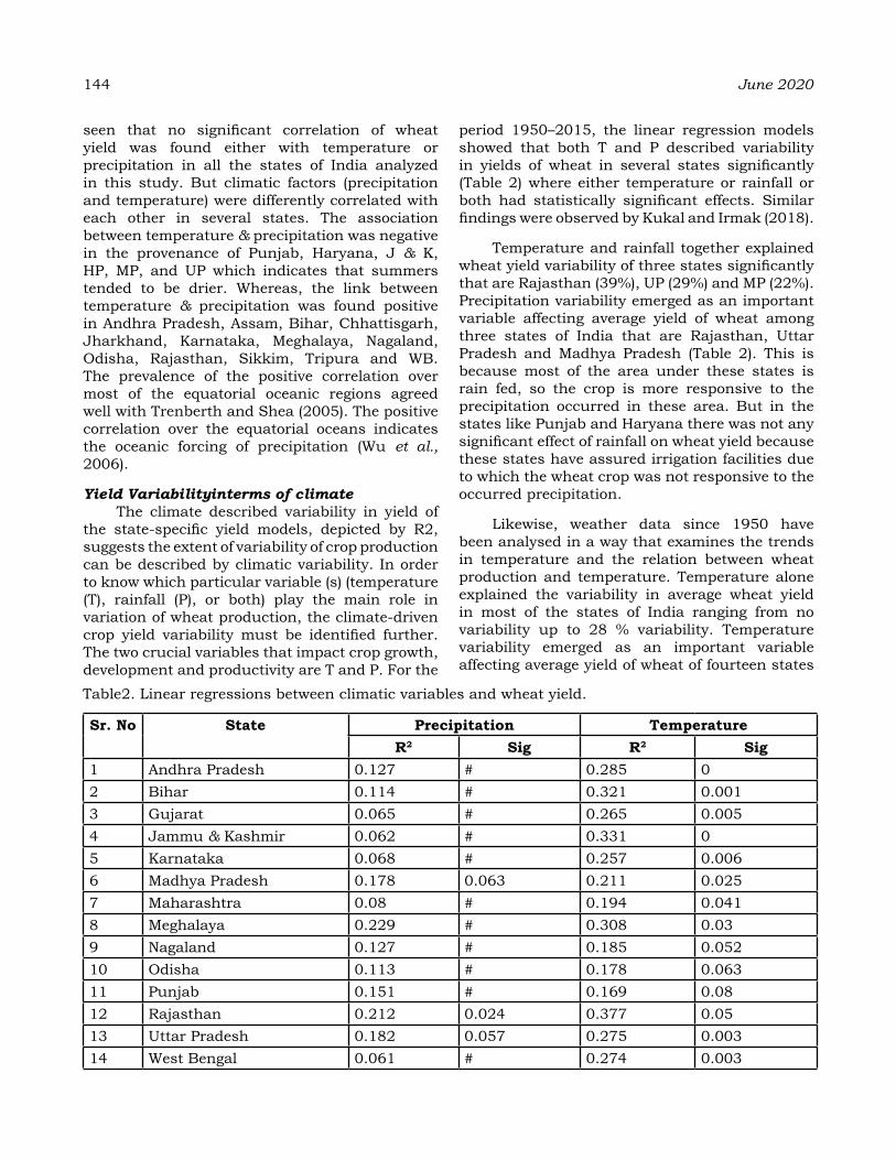
144 June 2020

seen that no significant correlation of wheat yield was found either with temperature or precipitation in all the states of India analyzed in this study. But climatic factors (precipitation and temperature) were differently correlated with each other in several states. The association between temperature & precipitation was negative in the provenance of Punjab, Haryana, J & K, HP, MP, and UP which indicates that summers tended to be drier. Whereas, the link between temperature & precipitation was found positive in Andhra Pradesh, Assam, Bihar, Chhattisgarh, Jharkhand, Karnataka, Meghalaya, Nagaland, Odisha, Rajasthan, Sikkim, Tripura and WB. The prevalence of the positive correlation over most of the equatorial oceanic regions agreed well with Trenberth and Shea (2005). The positive correlation over the equatorial oceans indicates the oceanic forcing of precipitation (Wu et al., 2006).

Yield Variabilityinterms of climateThe climate described variability in yield of

the state-specific yield models, depicted by R2, suggests the extent of variability of crop production can be described by climatic variability. In order to know which particular variable (s) (temperature (T), rainfall (P), or both) play the main role in variation of wheat production, the climate-driven crop yield variability must be identified further. The two crucial variables that impact crop growth, development and productivity are T and P. For the

period 1950–2015, the linear regression models showed that both T and P described variability in yields of wheat in several states significantly (Table 2) where either temperature or rainfall or both had statistically significant effects. Similar findings were observed by Kukal and Irmak (2018).

Temperature and rainfall together explained wheat yield variability of three states significantly that are Rajasthan (39%), UP (29%) and MP (22%). Precipitation variability emerged as an important variable affecting average yield of wheat among three states of India that are Rajasthan, Uttar Pradesh and Madhya Pradesh (Table 2). This is because most of the area under these states is rain fed, so the crop is more responsive to the precipitation occurred in these area. But in the states like Punjab and Haryana there was not any significant effect of rainfall on wheat yield because these states have assured irrigation facilities due to which the wheat crop was not responsive to the occurred precipitation.

Likewise, weather data since 1950 have been analysed in a way that examines the trends in temperature and the relation between wheat production and temperature. Temperature alone explained the variability in average wheat yield in most of the states of India ranging from no variability up to 28 % variability. Temperature variability emerged as an important variable affecting average yield of wheat of fourteen states

Table2. Linear regressions between climatic variables and wheat yield.

Sr. No State Precipitation temperatureR2 Sig R2 Sig

1 Andhra Pradesh 0.127 # 0.285 02 Bihar 0.114 # 0.321 0.0013 Gujarat 0.065 # 0.265 0.0054 Jammu & Kashmir 0.062 # 0.331 05 Karnataka 0.068 # 0.257 0.0066 Madhya Pradesh 0.178 0.063 0.211 0.0257 Maharashtra 0.08 # 0.194 0.0418 Meghalaya 0.229 # 0.308 0.039 Nagaland 0.127 # 0.185 0.05210 Odisha 0.113 # 0.178 0.06311 Punjab 0.151 # 0.169 0.0812 Rajasthan 0.212 0.024 0.377 0.0513 Uttar Pradesh 0.182 0.057 0.275 0.00314 West Bengal 0.061 # 0.274 0.003

of India namely J & K (26%), AP (28%), Bihar (25%), Gujarat (19%), Karnataka (18%), Meghalaya (19%), Maharashtra (11%), Madhya Pradesh (13%), Nagaland (10%), Odisha (9%), Punjab (8%), Rajasthan (26%), UP (20%) and WB (20%) variation respectively. The IPCC has affirmed that mean max and min temperatures have increased by 0.35 °C and 1.13 °C, respectively, mainly because of intensive agricultural practices, deforestation and industrialization etc. In the rabi season (January to April) a close connection between the grain yields of wheat and the mean minimum temperature was identified.

Peng et al., (2004) stated that, grain yield generally decreased by 10% for each 1 ° C rise in Tmin during the growing-period although negligible impacts of Tmax were observed in on yield. In comparison to the three variables described in the research, Leng et al., (2016) identified dominant climate variables which explained the crop yield variability in soybean and maize considerably; where they included seven promising combinations of climatic variables which can be allocated to any specific country.

Wheat Yield predictions in selected statesThe states having significant variability

of wheat yield explained by precipitation and temperature using regression model were further chosen to predict wheat yield. Hence, fourteen states were selected for ARIMA modelling. The aim of this analytical analysis is to build the best possible model of ARIMA crop yield predictor that best represents the cumulative effect of non-observed external crop variables. The following findings discuss our experimental studies to develop the crop yield forecasting model for various states of our country (Fig. 1). These climate patterns, either statistically significant or not, can have substantial effects on crop production by influencing yields, irrigation scheduling and crop water requirement, disease/pest risk, soil temperature, growing season duration, etc., and other crop and soil management activities and therefore require reasonable attention while assessing effect of climate change on crop production.

Fig. 1: The historical and predicted wheat productivity (in kg per hectare) in India for the period 1950-2025 for different states.


In the present analysis, using the 68-year time series results, the best fitted ARIMA models (Table 3), were used to predict up to 6 years of wheat in India. Based on its ability to predict using time series data with any kind of patterns and with auto-related successive values of the time series, the selected ARIMA models were used.The successive residuals in the fitted ARIMA models were also tested and statistically validated in the present analysis, and the residuals appear to be normally distributed at mean zero and constant variance. Hence, a satisfactory predictive model for wheat production in selected Indian provenance for the period 2019 to 2025 is given by the selected ARIMA model. The ARIMA models have predicted an increment in production in Punjab, Bihar, Gujarat, Karnataka, Odisha, Maharashtra and MP for a period of 6 years from 2019 to 2025 (Fig. 3, Table 4).


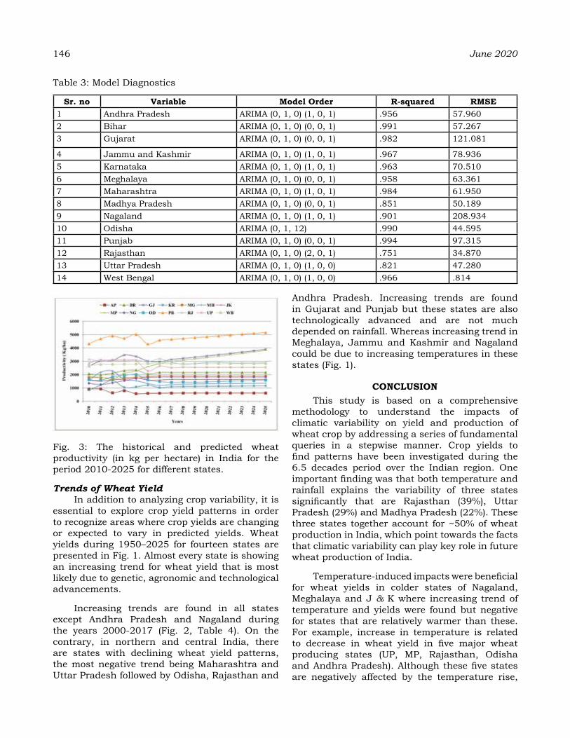
146 June 2020


Trends of Wheat YieldIn addition to analyzing crop variability, it is

essential to explore crop yield patterns in order to recognize areas where crop yields are changing or expected to vary in predicted yields. Wheat yields during 1950–2025 for fourteen states are presented in Fig. 1. Almost every state is showing an increasing trend for wheat yield that is most likely due to genetic, agronomic and technological advancements.

Increasing trends are found in all states except Andhra Pradesh and Nagaland during the years 2000-2017 (Fig. 2, Table 4). On the contrary, in northern and central India, there are states with declining wheat yield patterns, the most negative trend being Maharashtra and Uttar Pradesh followed by Odisha, Rajasthan and

Andhra Pradesh. Increasing trends are found in Gujarat and Punjab but these states are also technologically advanced and are not much depended on rainfall. Whereas increasing trend in Meghalaya, Jammu and Kashmir and Nagaland could be due to increasing temperatures in these states (Fig. 1).

CoNCLuSIoNThis study is based on a comprehensive

methodology to understand the impacts of climatic variability on yield and production of wheat crop by addressing a series of fundamental queries in a stepwise manner. Crop yields to find patterns have been investigated during the 6.5 decades period over the Indian region. One important finding was that both temperature and rainfall explains the variability of three states significantly that are Rajasthan (39%), Uttar Pradesh (29%) and Madhya Pradesh (22%). These three states together account for ~50% of wheat production in India, which point towards the facts that climatic variability can play key role in future wheat production of India.

Temperature-induced impacts were beneficial for wheat yields in colder states of Nagaland, Meghalaya and J & K where increasing trend of temperature and yields were found but negative for states that are relatively warmer than these. For example, increase in temperature is related to decrease in wheat yield in five major wheat producing states (UP, MP, Rajasthan, Odisha and Andhra Pradesh). Although these five states are negatively affected by the temperature rise,

Table 3: Model Diagnostics

Sr. no variable Model order r-squared rMSe1 Andhra Pradesh ARIMA (0, 1, 0) (1, 0, 1) .956 57.9602 Bihar ARIMA (0, 1, 0) (0, 0, 1) .991 57.2673 Gujarat ARIMA (0, 1, 0) (0, 0, 1) .982 121.081

4 Jammu and Kashmir ARIMA (0, 1, 0) (1, 0, 1) .967 78.9365 Karnataka ARIMA (0, 1, 0) (1, 0, 1) .963 70.5106 Meghalaya ARIMA (0, 1, 0) (0, 0, 1) .958 63.3617 Maharashtra ARIMA (0, 1, 0) (1, 0, 1) .984 61.9508 Madhya Pradesh ARIMA (0, 1, 0) (0, 0, 1) .851 50.1899 Nagaland ARIMA (0, 1, 0) (1, 0, 1) .901 208.93410 Odisha ARIMA (0, 1, 12) .990 44.59511 Punjab ARIMA (0, 1, 0) (0, 0, 1) .994 97.31512 Rajasthan ARIMA (0, 1, 0) (2, 0, 1) .751 34.87013 Uttar Pradesh ARIMA (0, 1, 0) (1, 0, 0) .821 47.28014 West Bengal ARIMA (0, 1, 0) (1, 0, 0) .966 .814

Maharashtra and Uttar Pradesh is most affected, followed by Odisha. The contribution of states to regional food production has been found to be a significant measure for the evaluation of the effects of climate.

reFereNCeSAggarwal, P. K. (2003). Impact of climate change

on Indian agriculture. Journal of Plant Biology. 30 (2) : 189-198.

Aggarwal, P.K. (2008). Global climate change and Indian agriculture: impacts adaptation and mitigation. Indian J.Agric. Sci. 78: 911−919.

Box, G. E. P., Jenkins, G. M., & Reinsel, G. C. (1994). Time series analysis, forecasting and control.Englewood Clifs.

CIMMYT (International Maize and Wheat Improvement Center). (2005). CIMMYT Business Plan 2006−2010 Translating the vision of seeds of innovation into a vibrant work plan. CIMMYT, Texcoco, p 31−37.

Easterling, D. R., Diaz, H. F., Douglas, A. V., Hogg, W. D., Kunkel, K. E., Rogers, J. C., and Wilkinson, J. F. (1999). Long term observation for monitoring extremes in the Americas. Climatic Change 42: 285-308.

Ewert, F., Rounsevell, M.D.A., Reginster, I., Metzger, M.G., Leemans, R. (2005). Future scenarios of European agricultural land use. I. Estimating changes in crop productivity. Agriculture, Ecosystem and Environment.

107:101–116.Fauchereau, N., Trzaska, M., Rouault, M. and

Richard, Y. (2003). Rainfall variability and changes in Southern Africa during the 20th century in the global warming context.Natural Hazards. 29: 139-154.

Gregory, P.J., Ingram, J.S.I., Brklacich, M. (2005). Climate change and food security.Philosophical Transactions of the Royal Society. 360: 2139–2148.

IPCC. (2001). Climate Change 2001 –The Scientific Basis, Contribution of Working Group I to the 3 Assessment Report of the Intergovernmental Panel on Climate Change. In: Houghton, J. T., Ding, Y., Griggs, D. J., Noguer, M., Van-der Linden P. J., Dai, X., Maskell K. and Johnson, C. A. (eds.), Cambridge University Press, UK. Pp. 881.

IPCC. (2007). Summary for Policy Makers. Climate Change 2007: The Physical Science Basis. Contribution of Working Group I to the Fourth Assessment Report. Cambridge University Press, Cambridge.

Jung, H. S., Choi, Y., Oh, J. H. and Lim, G. H. (2002). Recent trends in temperature and precipitation over South Korea’, International Journal of Climatology. 22: 1327-1337.

Kripalani R. H., Kulkarni, A., Sabade, S. S. and Khandekar, M. L. (2003). Indian monsoon

Table 4: Trends of wheat productivity (in kg per hectare) in India for the period 2000-2017 and 2010-2025.

Sr. no. States 2000-2017 2010-2025R2 y R2 Y

1 AP 0.1652 -15.132x + 850.51 0.3774 -14.386x + 783.322 BR 0.07 8.7025x + 1970.2 0.0482 3.8365x + 2122.63 GJ 0.7609 64.834x + 2100.9 0.7226 60.634x + 2798.24 KR 0.5029 33.353x + 601.89 0.0004 0.597x + 1134.65 MG 0.3312 12.644x + 1659.4 0.6748 9.1456x + 1772.86 MH 0.0572 14.723x + 1353.3 0.3833 -41.039x + 1824.57 JK 0.2762 15.925x + 1407.1 0.1245 3.5233x + 1602.38 MP 0.6146 66.071x + 1296.9 0.9562 147.35x + 1598.29 NG 0.2465 -39.296x + 2151.1 0.6311 32.784x + 1422.310 OD 0.2128 20.851x + 1293.5 0.2341 -17.959x + 1749.411 PB 0.1546 18.31x + 4329.5 0.4458 35.323x + 4488.612 RJ 0.6666 35.908x + 2528.2 0.5028 -16.929x + 3103.313 UP 0.013 4.9009x + 2723.3 0.453 -37.201x + 3007.814 WB 0.7176 44.631x + 2086.9 0.5703 6.1581x + 2748.5


148 June 2020

variability in a global warming scenarios. Natural Hazards. 29 (2) : 189-206.

Kukal, M.S. and Irmak, S. (2018). Climate-driven crop yield and yield variability and climate change impacts on the US great plains agricultural production. Sci. Rep. 8 (1) :3450.

Kumar, N.S., Aggarwal, P.K., Swaroopa Rani, D.N., Jain, S., Saxena, R., Chauhan, N. (2011).Impact of climate change on crop productivity in Western Ghats coastal and northeastern regions of India.Curr Sci. 101: 33−42

Kumar, N.S., Singh, A.K., Aggarwal, P.K., Rao, V.U.M., Venkateswarlu, B. (2012). Climate change and Indian agriculture: impact, adaptation and vulnerability-salient achievements from ICAR Network Project. Indian Agricultural Research Institute, New Delhi.

Kumar, N.S., Aggarwal, P.K, Saxena, R., Swaroopa Rani D.N., Jain, S., Chauhan, N. (2013).An assessment of regional vulnerability of rice to climate change in India.Clim Change. 118:683–699

Leng, G., Zhang, X., Huang, M., Asrar, G. R. & Leung, L. R. (2016).The Role of Climate Covariability on Crop Yields in the Conterminous United States. Sci. Rep. 6: 33160.

Lobell, D. B., Bänziger, M., Magorokosho, C. & Vivek, B. (2011). Nonlinear heat effects on African maize as evidenced by historical yield trials. Nature Climate Change.1: 42–45.

Monteith, J. (1980).Climatic variation and the growth of crops. Q. J. R. Meteor. Soc. 107: 749–774.

Pant, G. B., Kumar, R. and Borgaonkar, K. (1999). Climate and its long-term variability over the western Himalaya during the past two centuries. The Himalayan Environment (Eds. S. K. Dash and J. Bahadur), New Age International Limited, Publishers, Delhi. Pp. 172-184.

Panse, V. G. Sukhatme. (1985). Statistical methods for agricultural workers. ICAR, New Delhi.

Peng, S., Huang, J., Sheehy, J. E., Laza, R.

C., Visperas, R. M., Zhong, X., Centeno G.S., Khush G.S. and Cassman, K. G. (2004). Rice Yields Decline with Higher Night Temperature from Global Warming. Proceedings of the National Academy of Sciences of the United States of America.101 (27) : 9971-9975.

Sivakumar, M.V.K., Das, H.P., Brunini, O. (2005). Impacts of present and future climate variability and change on agriculture and forestry in the arid and semi-arid tropics.Climatic Change. 70:31–72.

Stephenson, B. Herve, D. D. and Rupakumar, K. (2001).Searching for a fingerprint of global warming in the Asian summer monsoon.Mausam. 52 (1) : 213-220.

Tao, S.Shen, S. Li, Y. Wang, Q. Gao, P. Mugume, I. (2016). Projected crop production under regional climate change using scenario data and modeling: Sensitivity to chosen sowing date and cultivar. Sustainability.8: 214.

Tao, F. Zhang, Z. (2013). Climate change, wheat productivity and water use in the North China Plain: A new super-ensemble based probabilistic projection. Agric. For. Meteorol. 170: 146–165.

Trenberth, K. E., and D. J. Shea. (2005). Relationships between precipitation and surface temperature.Geophys. Res. Lett. 32, L14703, doi:10.1029/2005GL022760

Tubiello, F.J., Donatelli, M., Rosenzweig, C., Stockle, C.O. (2000). Effects of climate change and elevated CO2 on cropping systems: model predictions at two Italian locations. European Journal of Agronomy. 13:179–189.

Wu, R., B. P. Kirtman, and K. Pegion, (2006). Local air-sea relationship in observations and model simulations. J. Climate.19: 4914–4932.

Wolf, J. (2002). Comparison of two potato simulation models underclimate change. I. Model calibration and sensitivity analyses. Climate Research. 21: 173–186.

Zhang, Q. Zhang, W. Li, T. Sun, W. Yu, Y. and Wang, G. (2017) Projective analysis of staple food crop productivity in adaptation to future climate change in China. Int. J. Biometeorol. 61: 1445–1460.

assessing the performance of wheat cultivars under present and futuristic climatic conditions using dSSat model

dIvYa1, K K gILL2, S S SaNdhu1, SaMaNPreet Kaur3, SS WaLIa4 aNd MaMta raNa5

1Department of Climate Change and Agricultural Meteorology2Communication Centre

3Department of Soil & Water Engineering4School of Organic Farming, Punjab Agricultural University, Ludhiana 141001, India

5CEEES, DCRUST S & T, Murthal, Sonipat, Haryana, IndiaCorresponding author: [email protected]

aBStraCtWheat is world’s second most important cereal crop and is vulnerable to thermal stress particularly in reproductive phase.A study was conducted to assess the implications of the future climatic change on wheat crop. The performance of three wheat cultivars viz. HD 2967, WH 1105 and PBW 590 sown on different dates i.e. 25th October, 15th November and 05th December was assessed by using crop growth simulation model (DSSAT version 4.6) in central Punjab. The DSSAT weather generator was used to get the futuristic data from 2010-2095. Among the 17 GCM models available, the best suitable model HADGEM-2E identified on the basis of NRMSE (Normalized root mean square error) and RMSE (Root mean square error) was used for the study. The futuristic data was taken using HADGEM-2E GCM model under scenarios RCP 4.5 and RCP 8.5 for mid-century (2020-50) and end century (2060-90) respectively. The comparison of bias was made between the modelled temperature data and the observed data for the five-year period (2010-14) and was removed by using linear scaling method. It has been found that under RCP 4.5, the mean annual temperature would increase by 1.4 oC (4.3 %) during MC and 3.0 oC (12.5%) during EC. Whereas, rainfall would increase by 217 mm (29%) and 185.5 mm (24%) during MC and EC, respectively. Similarly, under RCP 8.5, the mean annual temperature would increase by 1.4oC (6 %) during MC and 4.0oC (18%) during EC. The rainfall behaviour would increase by 120.41 mm (16%) and 255.6 mm (34%) during MC and EC, respectively. Under RCP 4.5, the grain yield in MC will reduce by 22.1, 25.0 and 16.8 percent for October, November and December sown cultivars, respectively. Similarly, in EC, the corresponding reductions will be 25.8, 17.1 and 10.5 percent. Under RCP 8.5, the grain yield in MC will reduce by 22.4, 21.6 and 16.2 percent for October, November and December sown cultivars, respectively. Similarly, in EC, the corresponding reductions will be 27.0, 15.9 and 6.6 percent.

Keywords: Wheat, DSSAT, Phenology, Crop modelling, HADGEM2-ES, Ludhiana (Punjab).

INtroduCtIoN

Wheat is one of the major crops of India. India’s share in global wheat production was 11.52 percent during the year 2018 (FAOSTAT, 2020). Punjab is leading wheat producing state in the country. In Punjab, wheat was grown over an area of 35 lac ha during 2015-16 with production of 160.7 lac tonnes and productivity of 16068 thousand metric ton (Statistical abstract of Punjab, 2016).

Wheat is a thermo-sensitive crop and therefore, choice of high yielding and disease resistant cultivars suitable to different sowing times is extremely important. In wheat, temperature above 300C after anthesis decreases the rate of grain filling. It was also predicted that an increase of 10C temperature will result in 4-5 million tons

(3-4%) of loss in wheat production (Wardlaw et al. 1989) Both sowing dates as well as irrigation are interrelated for better productivity. The timely sown wheat usually results in higher yields and escaped injury from drought, heat and diseases. The sowing of wheat in Punjab starts toward send of October and continues till first week of December. The normal growth and development of the crop primarily depends upon available irrigation water. Irrigation consistently increases wheat yield (Rahim et al.,2007), specifically when irrigation is applied at all definable growth stages (Wajid et al., 2002) but in the recent years due to changing climate these can be rescheduled according to the requirement of the crop.

In developing countries, drought, flood, heat and cold waves, will be increased in future (IPCC


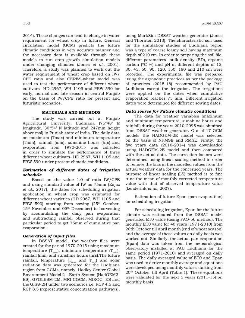
150 June 2020

2014). These changes can lead to change in water requirement for wheat crop in future. General circulation model (GCM) predicts the future climatic conditions in very accurate manner and the necessary data is available through these models to run crop growth simulation models under changing climates (Jones et al., 2001). Therefore, a study was planned to work out the water requirement of wheat crop based on IW/CPE ratio and also CERES-wheat model was used to test the performance of different wheat cultivars- HD 2967, WH 1105 and PBW 590 for early, normal and late season in central Punjab on the basis of IW/CPE ratio for present and futuristic scenarios.

MaterIaLS aNd MethodSThe study was carried out at Punjab

Agricultural University, Ludhiana (75°48’ E longitude, 30°54’ N latitude and 247mm height above msl) in Punjab state of India. The daily data on maximum (Tmax) and minimum temperature (Tmin), rainfall (mm), sunshine hours (hrs) and evaporation from 1970-2015 was collected in order to simulate the performance of three different wheat cultivars- HD 2967, WH 1105 and PBW 590 under present climatic conditions.

Estimation of different dates of irrigation schedule

Based on the value 1.0 of ratio IW/CPE and using standard value of IW as 75mm (Eajaz et al., 2017), the dates for scheduling irrigation application in wheat crop was estimated for different wheat varieties (HD 2967, WH 1105 and PBW 590) starting from sowing (25th October, 15th November and 05th December) to harvesting by accumulating the daily pan evaporation and subtracting rainfall observed during that particular period to get 75mm of cumulative pan evaporation.

Generation of input filesIn DSSAT model, the weather files were

created for the period 1970-2015 using maximum temperature (Tmax), minimum temperature (Tmin), rainfall (mm) and sunshine hours (hrs).The future rainfall, temperature (Tmax and Tmin) and solar radiation data was generated for the Ludhiana region from GCMs, namely, Hadley Center Global Environment Model 2 – Earth System (HadGEM2-ES), GFDLESM-2M, MRI-CGCM, MIROC- ES and the GISS-2H under two scenarios i.e. RCP 4.5 and RCP 8.5 (representative concentration pathways),

using MarkSim DSSAT weather generator (Jones and Thornton 2013). The characteristic soil used for the simulation studies of Ludhiana region was a type of coarse loamy soil having maximum depth of 210 cm. In order to preparing the soil file, different parameters- bulk density (BD), organic carbon (OC %) and pH at different depths of 15, 30, 45, 60, 90, 120, 150, 180 and 210 cm were recorded. The experimental file was prepared using the agronomic practices as per the package of practices (2015-16) recommended by PAU Ludhiana except the irrigation. The irrigations were applied on the dates when cumulative evaporation reaches 75 mm. Different irrigation dates were determined for different sowing dates.

Data source for Future climatic conditionsThe data for weather variables (maximum

and minimum temperature, sunshine hours and rainfall) during the years 2010-2095 was obtained from DSSAT weather generator. Out of 17 GCM models the HADGEM-2E model was selected on the basis of NRMSE and RMSE. Firstly, the five years data (2010-2014) was downloaded using HADGEM-2E model and then compared with the actual data. The correction factors were determined using linear scaling method in order to remove the bias in the modelled values from the actual weather data for the concerned years. The purpose of linear scaling (LS) method is to fine tune the mean of monthly corrected temperature value with that of observed temperature value (Lenderink et al., 2007).

Estimation of future Epan (pan evaporation) for scheduling irrigation

For scheduling irrigation, Epan for the future climate was estimated from the DSSAT model generated ET0 value (using FAO-56 method). The monthly ET0 value for 40 years (1971-2010) from 20th October till April month (end of wheat season) and the average of these values on daily basis was worked out. Similarly, the actual pan evaporation (Epan) data was taken from the meteorological observatory installed at PAU Ludhiana for the same period (1971-2010) and averaged on daily basis. The daily averaged value of ET0 and Epan was used to derive monthly average and equations were developed using monthly values starting from 20th October till April (Table 1). These equations were validated for the next 5 years (2011-15) on monthly basis.

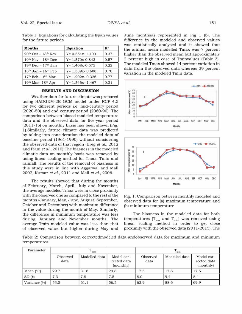
Table 1: Equations for calculating the Epan values for the future periods

Months equation R2

20th Oct – 18th Nov Y= 0.554x+1.403 0.3719th Nov – 18th Dec Y= 1.570x-0.843 0.5719th Dec – 17th Jan Y= 1.408x-0.575 0.2218th Jan – 16th Feb Y= 1.339x- 0.608 0.7017th Feb- 18th Mar Y= 1.202x- 0.326 0.7719th Mar- 18th Apr Y= 1.546x- 1.467 0.31

reSuLtS aNd dISCuSSIoNWeather data for future climate was prepared

using HADGEM-2E GCM model under RCP 4.5 for two different periods i.e. mid-century period (2020-50) and end century period (2060-90). The comparison between biased modeled temperature data and the observed data for five-year period (2011-15) on monthly basis has been shown (Fig. 1).Similarly, future climate data was predicted by taking into consideration the modeled data of baseline period (1961-1990) without considering the observed data of that region (Breg et al., 2012 and Piani et al., 2010).The biasness in the modeled climatic data on monthly basis was removed by using linear scaling method for Tmax, Tmin and rainfall. The results of the removal of biasness in this study were in line with Aggarwal and Mall 2002, Kumar et al., 2011 and Mall et al., 2006.

The results showed that during the months of February, March, April, July and November, the average modeled Tmax were in close proximity with the observed one as compared to the rest of the months (January, May, June, August, September, October and December) with maximum difference in the value during the month of May. Similarly, the difference in minimum temperature was less during January and November months. The average Tmin modeled value was less than that of observed value but higher during May and

June monthsas represented in Fig 1 (b). The difference in the modeled and observed values was statistically analysed and it showed that the annual mean modelled Tmax was 7 percent higher than the observed mean but approximately 2 percent high in case of Tminvalues (Table 3). The modeled Tmax showed 14 percent variation in data from the observed data whereas 39 percent variation in the modeled Tmin data.

Fig. 1: Comparison between monthly modeled and observed data for (a) maximum temperature and (b) minimum temperature

The biasness in the modeled data for both temperatures (Tmax and Tmin) was removed using linear scaling method in order to get close proximity with the observed data (2011-2015). The

Table 2: Comparison between correctedmodeled data andobserved data for maximum and minimum temperatures

Parameter Tmax Tmin

Observed data

Modelled data Model cor-rected data (monthly)

Observed data

Modelled data Model cor-rected data (monthly)

Mean (°C) 29.7 31.8 29.8 17.5 17.8 17.5SD (±) 7.3 7.8 7.5 8.0 9.4 8.4Variance (%) 53.5 61.1 56.5 63.9 88.6 69.9

Vol. 22, Special Issue DIVYA et al. 151

152 June 2020

unbiased results were statistically analysed and it has been found that the difference in the mean modeled value of corrected Tmax has reduced to approx. 2 percent less as compared to 5 percent in case of mean biased modeled value from the observed value. Whereas, the mean (µ) corrected modeled value of Tmin showed even less than 2 percent value than the observed mean (µ) value (Table 2).

The temperature has been changing continuously due to various effects such as global warming. Table 3 showed the change in temperature in future years i.e. MC (2020-50) and EC (2060-90) and compared with the present observed period (1970-2015) under RCP 4.5 and RCP 8.5 (IPCC, 2014).Under RCP 4.5, ithas been observed that during MC the Tmax increased by 3.7% whereas 10% during EC. While, the Tmin increased by 9.6% during MC and 16% during EC. The mean increase in temperature would be 6% and 12.5% during MC and EC. Similarly, total rainfall also showed increase by 28.6% and 24.4% during MC and EC, respectively. Similarly, Under RCP 8.5, the hike in Tmax was less than 4.5 scenario i.e. 3.0% during MC whereas 12% during EC. However, the rise in Tmin has been observed to be much more than expected i.e. by 10.8% during MC and 27% during EC. The mean increase in temperature would be 6% and 17.7% during MC and EC, respectively. Similarly, total rainfall has also shown rising scenario and would increase by 16% and 33.7% during MC and EC,

respectively.

Table 3: Change in the future annual maximum, minimum temperature and rainfall data formid-century and end century under RCP 4.5 and RCP 8.5

Tem-pera-ture (°C)

Ob-served (1970-2015)

RCP 4.5 RCP 8.5MC

(2020-50)

EC (2060-

90)

MC (2020-

50)

EC (2060-

90) Tmax 29.8 30.9 32.8 30.7 33.4Tmin 16.7 18.3 19.4 18.5 21.2Mean 23.2 24.6 26.1 24.6 27.3Rain 759.3 976.2 944.8 880.2 1015.4

Effect of climate change on the phenology, irrigation requirement and yield of wheat cultivars

The phenology, irrigation requirement (mm) and wheat yield (kg/ha) were worked out for different wheat cultivars under observed, MC and EC period for both the scenarios i.e. RCP 4.5 and RCP 8.5 (Table 6 and 7).The cultivar WH 1105 showed the highest average yield of 6017 kg/ha with the least irrigation requirement during observed period. All the cultivars performed the best during the observed period. Whereas, during MC, the average yield of HD 2967 and WH 1105 were at par with a difference of 156 kg and almost same irrigation requirement of 220 mm but PBW 590 showed the lower yield than other cultivars. During EC, WH 1105 showed highest average

Table 4: Effect of different time periods on phenology, irrigation requirement and yield of different wheat cultivars under RCP 4.5

Parame-ters

Wheat varietiesObserved period MC EC

HD 2967 (25th Oc-

tober)

WH 1105 (15th No-vember)

PBW 590 (05th De-cember)

HD 2967 (25th Oc-

tober)



HD 2967 (25th Oc-

tober)



Days to anthesis

119 107 93 110 102 91 104 100 89

Days to maturity

154 140 122 145 133 118 139 130 115

Irrigation require-ment (mm)

196 173 176 220 220 199 290 283 256

Wheat yield (kg/ha)

5990 6017 5083 4666 4510 4230 4443 4989 4547

yield of 4989 kg/ha with less irrigation demand than HD 2967. Under RCP 4.5, November sown cultivar WH 1105 showed the best result than the other cultivars and time of sowing. Under RCP 8.5, during MC, the average yield was highest for November cultivar WH 1105 than the other cultivars although its irrigation requirement was more than October sown HD 2967 (Table 7). Similarly, during EC, November sown cultivar WH 1105 showed the highest yield of 5060 kg/ha and the irrigation requirement for all the cultivars was same. Under RCP 8.5, November sown cultivar WH 1105 showed the best results during MC and EC. Aitkur et al. (2018) also predicted 5.32ºC increase in temperature in the year 2100 for the north-central region of Bangladesh and decrease in yieldof wheat, rice and potato by 47.6%, 67.8% and 38.6%, respectively. The increased temperature would accelerate physiological maturity of the crops as reflected by their reduced length of growing season (LGS) by 1.20% to 18.5%. The reduced LGS would reduce seasonal evapotranspiration (ET) of the crops by shortening time-span for ET generation.

CoNCLuSIoNIt has been found that increased temperature

shortened the crop duration. Under RCP 4.5, the days to anthesis would decrease by 2-9 days for different cultivars sown from October to December during MC. Whereas, days to anthesis decreased by 15, 7- and 4-days during EC. Similarly, the days to physiological maturity also reduced by 4-9 days for October sown to December sown

cultivars during MC. Where as days to anthesis decreased by 15, 10 and 7 days during EC under RCP 4.5. Under RCP 8.5, the anthesis period would be shortened by 9, 5 and 1days during MC which were almost close to RCP 4.5 but during EC it would decrease by 21, 11 and 6 days. The days to physiological maturity would also shorten by 8 days for October sown cv. HD 2967, 6 days for November sown cv. WH 1105 and 3 days for December sown cv. PBW 590 during MC. Whereas, during EC the days to maturity would shorten by 21 days, 14 days and 11 days for October, November and December sown cultivars. Under RCP 4.5, the grain yield in MC will reduce by 22.1, 25.0 and 16.8 percent for October, November and December sown cultivars, respectively. Similarly, in EC, the corresponding reductions will be 25.8, 17.1 and 10.5 percent. Under RCP 8.5, the grain yield in MC will reduce by 22.4, 21.6 and 16.2 percent for October, November and December sown cultivars, respectively. Similarly, in EC, the corresponding reductions will be 27.0, 15.9 and 6.6 percent. The findings of this study expose a potential risk for food security in the major food growing region (Punjab) in India. This risk poses serious consequences for agriculture and related sectors in addition with diminishing crop lands and increasing population. Therefore, there is need of consideration of results from this study and of similar others for better planning in the changing and variable climate as coping mechanisms such as change in current cropping practices or developing new resistant varieties.

Table 5: Effect of different time periods on phenology, irrigation requirement and yield of different wheat cultivars under RCP 8.5

Parame-ters

Wheat varietiesObserved period MC EC

HD 2967 (25th Oc-

tober)



HD 2967 (25th Oc-

tober)



HD 2967 (25th Oc-

tober)



Days to anthesis

119 107 93 110 102 92 98 96 87

Days to maturity

154 140 122 146 134 119 133 126 111

Irrigation require-ment (mm)

196 173 176 225 266 246 300 300 300

Wheat yield (kg/ha)

5990 6017 5083 4650 4715 4260 4370 5060 4750

Vol. 22, Special Issue DIVYA et al. 153

154 June 2020

reFereNCeSAggarwal, P. K. and Mall, R. K. (2002). Climate

change and rice yields in diverse agro- environments of India. 2. Effect of uncertainties in scenarios and crop models on impact assessments. Climate Change 52: 331-43.

Berg, P., Fieldmann, H. and Panitz, H. J. (2012). Bias correction of high-resolution regional climate change model data. J. Hydrol., 448: 80-92.

Eajaz Ahmad Dara, A.S. Brara, S.K. Mishrab and K.B. Singh. (2017). Simulating response of wheat to timing and depth of irrigation water in drip irrigation system using CERES-Wheat model. Field Crops Res., 214:149-163.

FAOSTAT. (2018). Cited fromhttp://www.fao.org/faostat/en/#data/QC.

IPCC, Climate Change. (2014). Impacts, adaptation and vulnerability. Part A: Global and sectorial aspects. Contribution of Working group II to the Fifth Assessment Reportof Intergovernmental Panel on Climate Change.

Jones, J. W., Keating, B. A. and Porter, C. H. (2001). Approaches to modular model development. J. Agri. Systems, 70: 421-43.

Jones, P. G. And Thoronton, P. K. (2013). Generating downscaled weather data from a suite of climate models for agricultural modelling applications. Int. J. Agri. Syst., 114: 1-5.

Kumar, K. K., Patwardan, S. K., Kulkarni, A., Kamala, K., Rao, K. and Jones. (2011). Simulated projections for summer monsoon climate over India by a high-resolution regional climate model (PRECIS). Current Sci., 101 (3) : 312-26.

Leanderink, G., Buishand, A. and Van, Deursen W. (2007). Estimates of future discharges of the river Rhine using two scenario

methodologies: direct versus delta approach. J. Hydrol. EarthSyst.Sci., 11: 1145-59.

Mall, R. K., Lal, M., Bhatia, V. S., Rathore, L. S. and Singh, R. (2004). Mitigating climate change impact on soyabean productivity in India: a simulation study. Agri. For. Meteorol., 121 (1-2) : 113-25.

Piani, C. J. O., Haerter and Coppola, E. (2010) Statistical bias correction for daily precipitation in regional climate models over Europe. J. Theor. Appl. Climatol., 99: 187-92.

Rahim, A., Abbassi, G. H., Rashid, M. and Ranjha, A. M. (2007). Methods of phosphorus application and irrigation schedule influencing wheat yield. Pak. J. Agric.Sci., 44: 420- 23.

Rahman A, Mojid M A and Banu S (2018). Climate change impact assessment on three major crops in the north-central region of Bangladesh using DSSAT. Int J Agric & BiolEng, 11 (4) : 135–14

Statistical Abstract of Punjab. (2016).Cited from https://www.worldcat.org/title/statistical-abstract-of-punjab/oclc/1645812

Wajid, A., Hussain, A., Maqsood, M., Ahmad, A. and Awais, M. (2002). Influence of sowing date and irrigation levels on growth and grain yield of wheat. Pak. J. Agric.Sci., 39: 22-24.

Wardlaw, IF., Dawson IA. and Munibi, P. (1989). The tolerance of wheat to high temperatures during reproductive growth: II Grain development. Australian Journal of Agricultural Research. 40: 15-24.

Xiao, D., Tao, F., Liu, Y., Shi, W., Wang, M., Liu, F., Zhang, S. and Zhu, Z. (2013). Observed changes in winter wheat phenology in the North China Plain. Int. J. Biometeorol., 57 (2) : 275-85.

Change in timing of occurrence of temperature extremes in central Punjab

S. S. SaNdhu1, PraBhJYot-Kaur1 aNd K. K. gILL2

1Department of Climate Change and Agricultural Meteorology, Punjab Agricultural University, Ludhiana, Punjab, India (141004)

2Communication Centre, Punjab Agricultural University, Ludhiana, Punjab, India (141004) *Corresponding author email: [email protected]

aBStraCtTemperature and its extreme are detrimental for all living organisms. There are some indications of shift in the occurrence of the extremes of temperatures. A study was conducted to analyze the shifts in timing of occurrence of temperature extremes in central Punjab. The daily maximum and minimum temperature data (1970-2017) recorded at PAU; Ludhiana was used for the study. The days with highest temperatures were determined from the temperature recorded between 1st March to 31st August and days of lowest temperature were determined from 1st December (preceding year) through 28th February. The results revealed an increase in number of days having highest value of maximum temperature in May and number of such days has decreased in June. On the other hand the number of days of lowest average temperature have increased in January and decreased in February. The trend analysis revealed that there was a shift towards early occurrence of days having highest value of maximum temperature and the rate of shift was 0.32 days per year and similar early occurrence of days having lowest value of average temperature was also observed and the rate of shift was 0.46 days per year. The study clearly indicated that there is a shift in time of occurrence of temperature extremes in central Punjab and it may adversely affect the crops and water balance in the region.

Keywords: Temperature, extreme, change, time, shift, early

INtroduCtIoN

Temperature is an important weather parameters affecting agriculture. Its extreme values are detrimental for the living organisms. Most of the climate change studies (Mondal et al., 2015; Prabhjyot-Kaur et al., 2013) have focused on analyzing the quantum of change or the rate of change of the temperature. There are some studies that evaluated the changes in extreme daily temperatures (Dash and Mamgain 2011). Studies (De and Mukhopadhyay, 1998; Pai et al., 2004; Bhuarya et al., 2017) are available suggesting that the heat and cold waves in India have increased in recent years. Heat waves are harmful and these are mostly experienced in Southern and Central India from March to May. Its effects may include shedding of leaves, fruits, water loss by evaporation from reservoirs, increase in transpiration, drying of water resources and all these may lead to stresses in crops. Floods, droughts, heat waves / cold waves and associated weather phenomena have caused several deaths in the past (Kaur et al., 2015). Human life and the environment are being impacted by extreme weather events such as heat waves, lightning, floods, and rising temperatures (Min et al., 2011; Jahn, 2015). In general for kharif

crops, temperature is not a major constraint but sudden rise or fall in temperature, low or high rainfall, low sunshine hours are constraints for many kharif crops (Kaur et al., 2015).

Literature is lacking in studies related to change in the time of occurrence of extreme temperatures. Such changes can have greater impact on agriculture including crops, vegetables and livestock. Thus, studying the climate change from a different angle other than the change in value or the rate of change of weather parameter is important socially and economically for India There are indications of shift in the time of occurrence of the extremes of temperatures. Therefore, a study was executed with an objective to determine any shift in time (date) of occurrence of temperature extremes in Ludhiana district of Indian Punjab.

MaterIaLS aNd MethodSData used

The daily maximum and minimum temperature data (1970-2017) recorded at Agrometeorological Observatory, Punjab Agricultural University, Ludhiana was used for the study.


156 June 2020

Temperature data analysisThe daily maximum, minimum and average

temperature data was used for determination of extremes on both higher and lower sides. Extremes on higher sides represented hot days, while, extremes on lower side represented colder days. The temperature data from 1st March to 31st August was used to determine days having highest value of maximum, minimum and average temperatures (Table 1). The temperature data from 1st December (preceding year) through 28th February was used to

determine days having lowest value of maximum, minimum and average temperatures (Table 2). The highest and lowest values of maximum, minimum and average temperatures were determined by using conditional formatting function available in Microsoft Excel.

The yearly highest and lowest values of maximum, minimum and average temperatures were grouped on decadal basis and the last eight years (2010-2017) were taken into consideration

Table 1: Decadal analysis of days with highest values of temperature

decade day with highest value ofMaximum temperature Minimum temperature average temperature

1970-79

19 May 1970 28 June 1970 19 May 197013 June 1971 23 August 1971 13 June 197114 June 1972 18 June 1972 18 June 19726 June 1973 31 August 1973 7 June 197315 June 1974 17 June 1974 16 June 197416 June 1975 18 June 1975 17 June 197528 June 1976 13 July 1976 29 June 19764 June 1977 23 June 1977 22 June 19773 June 1978 25 May 1978 7 June 19789 June 1979 26 June 1979 29 June 1979

1980-89

12 May 1980 10 June 1980 10 June 198017 June 1981 28 June 1981 21 June 198110 July 1982 1 July 1982 13 June 198223 June 1983 1 August 1983 20 July 198324 May 1984 27 May 1984 27 May 198430 May 1985 23 June 1985 23 June 198510 June 1986 18 June 1986 18 June 19867 June 1987 24 July 1987 3 July 198725 May 1988 27 June 1988 31 May 198816 May 1989 12 July 1989 3 June 1989

1990-99

28 May 1990 25 June 1990 18 June 199025 May 1991 3 June 1991 3 June 19916 June 1992 20 June 1992 19 June 199225 May 1993 23 June 1993 7 June 19939 June 1994 9 June 1994 9 June 19948 June 1995 5 August 1995 16 June 199529 May 1996 4 June 1996 29 May 199616 June 1997 18 June 1997 18 June 199726 May 1998 28 May 1998 26 May 19981 May 1999 26 June 1999 4 May 1999

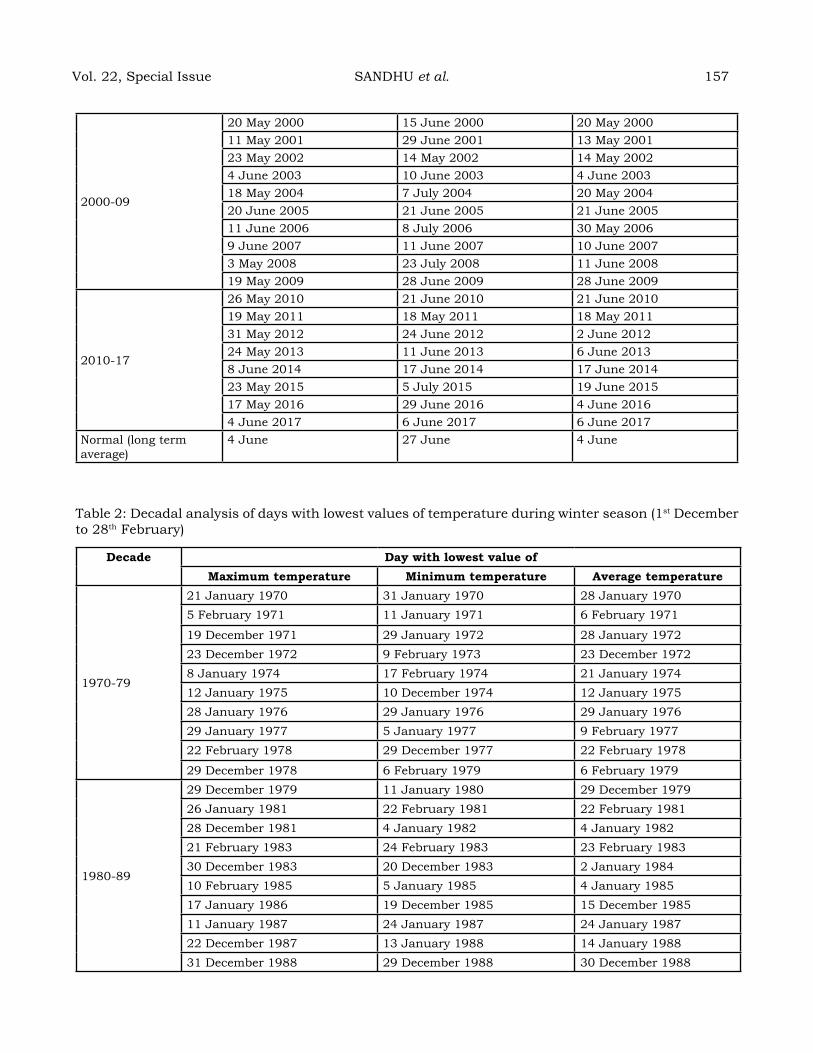
2000-09

20 May 2000 15 June 2000 20 May 200011 May 2001 29 June 2001 13 May 200123 May 2002 14 May 2002 14 May 20024 June 2003 10 June 2003 4 June 200318 May 2004 7 July 2004 20 May 200420 June 2005 21 June 2005 21 June 200511 June 2006 8 July 2006 30 May 20069 June 2007 11 June 2007 10 June 20073 May 2008 23 July 2008 11 June 200819 May 2009 28 June 2009 28 June 2009

2010-17

26 May 2010 21 June 2010 21 June 201019 May 2011 18 May 2011 18 May 201131 May 2012 24 June 2012 2 June 201224 May 2013 11 June 2013 6 June 20138 June 2014 17 June 2014 17 June 201423 May 2015 5 July 2015 19 June 201517 May 2016 29 June 2016 4 June 20164 June 2017 6 June 2017 6 June 2017

Normal (long term average)

4 June 27 June 4 June

Table 2: Decadal analysis of days with lowest values of temperature during winter season (1st December to 28th February)

decade day with lowest value ofMaximum temperature Minimum temperature average temperature

1970-79

21 January 1970 31 January 1970 28 January 19705 February 1971 11 January 1971 6 February 1971

19 December 1971 29 January 1972 28 January 197223 December 1972 9 February 1973 23 December 19728 January 1974 17 February 1974 21 January 197412 January 1975 10 December 1974 12 January 197528 January 1976 29 January 1976 29 January 197629 January 1977 5 January 1977 9 February 197722 February 1978 29 December 1977 22 February 1978

29 December 1978 6 February 1979 6 February 1979

1980-89

29 December 1979 11 January 1980 29 December 197926 January 1981 22 February 1981 22 February 198128 December 1981 4 January 1982 4 January 198221 February 1983 24 February 1983 23 February 198330 December 1983 20 December 1983 2 January 198410 February 1985 5 January 1985 4 January 198517 January 1986 19 December 1985 15 December 198511 January 1987 24 January 1987 24 January 198722 December 1987 13 January 1988 14 January 198831 December 1988 29 December 1988 30 December 1988

Vol. 22, Special Issue SANDHU et al. 157

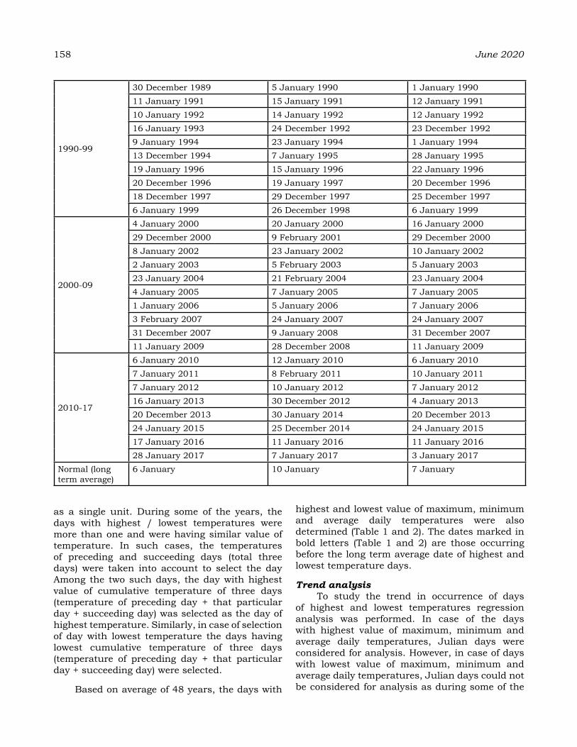
158 June 2020

as a single unit. During some of the years, the days with highest / lowest temperatures were more than one and were having similar value of temperature. In such cases, the temperatures of preceding and succeeding days (total three days) were taken into account to select the day Among the two such days, the day with highest value of cumulative temperature of three days (temperature of preceding day + that particular day + succeeding day) was selected as the day of highest temperature. Similarly, in case of selection of day with lowest temperature the days having lowest cumulative temperature of three days (temperature of preceding day + that particular day + succeeding day) were selected.

Based on average of 48 years, the days with

highest and lowest value of maximum, minimum and average daily temperatures were also determined (Table 1 and 2). The dates marked in bold letters (Table 1 and 2) are those occurring before the long term average date of highest and lowest temperature days.

Trend analysisTo study the trend in occurrence of days

of highest and lowest temperatures regression analysis was performed. In case of the days with highest value of maximum, minimum and average daily temperatures, Julian days were considered for analysis. However, in case of days with lowest value of maximum, minimum and average daily temperatures, Julian days could not be considered for analysis as during some of the

1990-99

30 December 1989 5 January 1990 1 January 199011 January 1991 15 January 1991 12 January 199110 January 1992 14 January 1992 12 January 199216 January 1993 24 December 1992 23 December 19929 January 1994 23 January 1994 1 January 199413 December 1994 7 January 1995 28 January 199519 January 1996 15 January 1996 22 January 199620 December 1996 19 January 1997 20 December 199618 December 1997 29 December 1997 25 December 19976 January 1999 26 December 1998 6 January 1999

2000-09

4 January 2000 20 January 2000 16 January 200029 December 2000 9 February 2001 29 December 20008 January 2002 23 January 2002 10 January 20022 January 2003 5 February 2003 5 January 200323 January 2004 21 February 2004 23 January 20044 January 2005 7 January 2005 7 January 20051 January 2006 5 January 2006 7 January 20063 February 2007 24 January 2007 24 January 200731 December 2007 9 January 2008 31 December 200711 January 2009 28 December 2008 11 January 2009

2010-17

6 January 2010 12 January 2010 6 January 20107 January 2011 8 February 2011 10 January 20117 January 2012 10 January 2012 7 January 201216 January 2013 30 December 2012 4 January 201320 December 2013 30 January 2014 20 December 201324 January 2015 25 December 2014 24 January 201517 January 2016 11 January 2016 11 January 201628 January 2017 7 January 2017 3 January 2017

Normal (long term average)

6 January 10 January 7 January

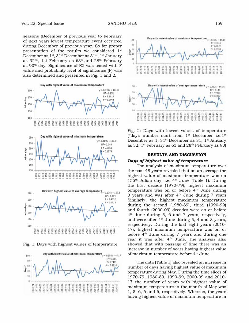
seasons (December of previous year to February of next year) lowest temperature event occurred during December of previous year. So for proper presentation of the results we considered 1st December as 1st, 31st December as 31st, 1st January as 32nd, 1st February as 63rd and 28th February as 90th day. Significance of R2 was tested with F value and probability level of significance (P) was also determined and presented in Fig. 1 and 2.

Fig. 1: Days with highest values of temperature

Fig. 2: Days with lowest values of temperature (*days number start from 1st December i.e.1st December as 1, 31st December as 31, 1st January as 32, 1st February as 63 and 28th February as 90)

reSuLtS aNd dISCuSSIoNDays of highest value of temperature

The analysis of maximum temperature over the past 48 years revealed that on an average the highest value of maximum temperature was on 155th Julian day, i.e. 4th June (Table 1). During the first decade (1970-79), highest maximum temperature was on or before 4th June during 3 years and was after 4th June during 7 years Similarly, the highest maximum temperature during the second (1980-89), third (1990-99) and fourth (2000-09) decades were on or before 4th June during 5, 6 and 7 years, respectively, and were after 4th June during 5, 4 and 3 years, respectively. During the last eight years (2010-17), highest maximum temperature was on or before 4th June during 7 years and during one year it was after 4th June. The analysis also showed that with passage of time there was an increase in number of years having highest value of maximum temperature before 4th June.

The data (Table 1) also revealed an increase in number of days having highest value of maximum temperature during May. During the time slices of 1970-79, 1980-89, 1990-99, 2000-09 and 2010-17 the number of years with highest value of maximum temperature in the month of May was 1, 5, 6, 6 and 6, respectively. Whereas, the years having highest value of maximum temperature in


160 June 2020

June during the time slices of 1970-79, 1980-89, 1990-99, 2000-09 and 2010-17 were 9, 4, 4, 4 and 2, respectively. Hence, over the past 48 years the days with highest value of maximum temperature have decreased during June and increased during May month at Ludhiana.

The analysis of minimum temperature over the past 48 years revealed that on an average the highest value of minimum temperature was on 178th Julian day, i.e. 27th June (Table 1).During the first decade (1970-79), highest minimum temperature was before 27th June during 6 years and was after 27th June during 4 years. Similarly, the highest minimum temperature during the second (1980-89), third (1990-99) and fourth (2000-09) decades were on or before 27th June during 5, 9 and 5 years, respectively, and were after 27th June during 5, 1 and 5 years, respectively. During the last eight years (2010-17), highest minimum temperature was before 27th June during 6 years and during 2 year it was after 27th June.

The analysis of daily average temperature over the past 48 years revealed that on an average the highest value of daily average temperature was on 155th Julian day, i.e. 4th June (Table 1) which was same as that in case of maximum temperature. During the first decade (1970-79), highest daily average temperature was before 4th June during one year and was after 4th June during 9 years. Similarly, the highest daily average temperature during the second (1980-89), third (1990-99) and fourth (2000-09) decades were on or before 4th June during 3, 4 and 6 years, respectively, and were after 4th June during 7, 6 and 4 years, respectively. During the last eight years (2010-17), highest daily average temperature was on or before 4th June during 3 years and during 5 year it was after 4th June. The analysis also revealed that there was an increase in number of years (6) having highest value of average temperature on or before 4th June up to 2000-09 and thereafter it decreased to 3 in the last 8 years.

These changes in time of occurrence of highest value of temperature may affect the crop productivity. The crops in their reproductive phase may get more affected due to failure of fertilization as Sakata and Higashitani, (2008) and Wassmann et al., (2009) observed that altered pollen development and male sterility, in response to heat stress, are the major reasons for reduction in productivity. Zhao et al., (2017) reported that

each degree-Celsius increase in earth’s mean temperature will lead to a decrease in global yields of wheat, rice, maize and soybean by 6.0, 3.2, 7.4 and 3.1 per cent. The impacts of high temperature on crops have been discussed in details by Sandhu et al., (2018).

Days of lowest value of temperature The analysis of maximum temperature over

the past 48 years revealed that on an average the lowest value of maximum temperature was on 6th Julian day, i.e. 6th January (Table 2). During the first decade (1970-79), lowest maximum temperature was before 6th January during 3 years and was after 6th January during 7 years. Similarly, the lowest maximum temperature during the second (1980-89), third (1990-99) and fourth (2000-09) decades were on or before 6th January during 5, 5 and 6 years, respectively, and were after 6th January during 5, 5 and 4 years, respectively. During the last eight years (2010-17), lowest maximum temperature was on or before 6th January during 2 years and during 6 years it was after 6th January. The analysis showed an increase in number of days having lowest value of maximum temperature before 6th January upto 2000-09 and thereafter it decreased.

The analysis of minimum temperature over the past 48 years revealed that on an average the lowest value of minimum temperature was on 10th Julian day, i.e. 10th January (Table 2). During the first decade (1970-79), lowest minimum temperature was before 10th January during 4 years and was after 10th January during 6 years. Similarly, the lowest minimum temperature during the second (1980-89), third (1990-99) and fourth (2000-09) decades were before 10th January during 5, 5 and 4 years, respectively, and were after 10th January during 5, 5 and 6 years, respectively. During the last eight years (2010-17), lowest minimum temperature was on or before 10th January during 4 years and during remaining 4 year it was after 10th January.

The analysis of daily average temperature over the past 48 years revealed that on an average the lowest value of daily average temperature was on 7th Julian day, i.e. 7th January (Table 2). During the first decade (1970-79), lowest daily average temperature was before 7th January during one year and was after 7th January during 9 years. Similarly, the lowest daily average temperature during the second (1980-89), third (1990-99) and fourth (2000-09) decades were on or before 7th

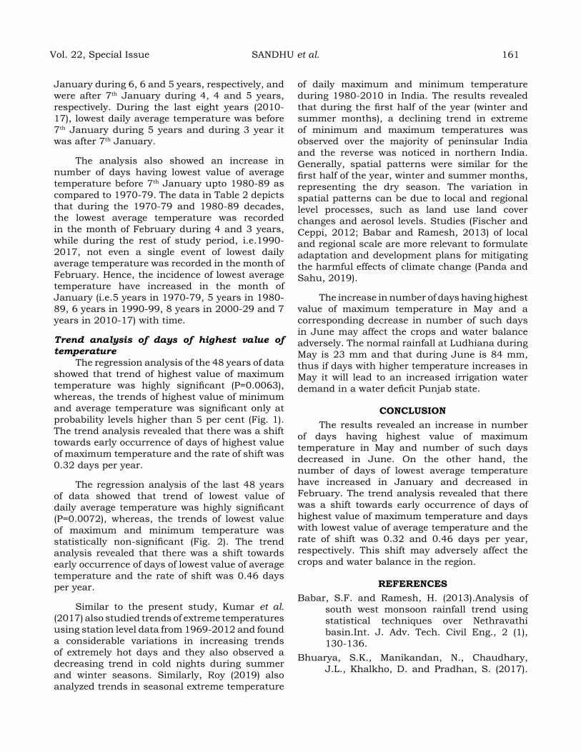
January during 6, 6 and 5 years, respectively, and were after 7th January during 4, 4 and 5 years, respectively. During the last eight years (2010-17), lowest daily average temperature was before 7th January during 5 years and during 3 year it was after 7th January.

The analysis also showed an increase in number of days having lowest value of average temperature before 7th January upto 1980-89 as compared to 1970-79. The data in Table 2 depicts that during the 1970-79 and 1980-89 decades, the lowest average temperature was recorded in the month of February during 4 and 3 years, while during the rest of study period, i.e.1990-2017, not even a single event of lowest daily average temperature was recorded in the month of February. Hence, the incidence of lowest average temperature have increased in the month of January (i.e.5 years in 1970-79, 5 years in 1980-89, 6 years in 1990-99, 8 years in 2000-29 and 7 years in 2010-17) with time.

Trend analysis of days of highest value of temperature

The regression analysis of the 48 years of data showed that trend of highest value of maximum temperature was highly significant (P=0.0063), whereas, the trends of highest value of minimum and average temperature was significant only at probability levels higher than 5 per cent (Fig. 1). The trend analysis revealed that there was a shift towards early occurrence of days of highest value of maximum temperature and the rate of shift was 0.32 days per year.

The regression analysis of the last 48 years of data showed that trend of lowest value of daily average temperature was highly significant (P=0.0072), whereas, the trends of lowest value of maximum and minimum temperature was statistically non-significant (Fig. 2). The trend analysis revealed that there was a shift towards early occurrence of days of lowest value of average temperature and the rate of shift was 0.46 days per year.

Similar to the present study, Kumar et al. (2017) also studied trends of extreme temperatures using station level data from 1969-2012 and found a considerable variations in increasing trends of extremely hot days and they also observed a decreasing trend in cold nights during summer and winter seasons. Similarly, Roy (2019) also analyzed trends in seasonal extreme temperature

of daily maximum and minimum temperature during 1980-2010 in India. The results revealed that during the first half of the year (winter and summer months), a declining trend in extreme of minimum and maximum temperatures was observed over the majority of peninsular India and the reverse was noticed in northern India. Generally, spatial patterns were similar for the first half of the year, winter and summer months, representing the dry season. The variation in spatial patterns can be due to local and regional level processes, such as land use land cover changes and aerosol levels. Studies (Fischer and Ceppi, 2012; Babar and Ramesh, 2013) of local and regional scale are more relevant to formulate adaptation and development plans for mitigating the harmful effects of climate change (Panda and Sahu, 2019).

The increase in number of days having highest value of maximum temperature in May and a corresponding decrease in number of such days in June may affect the crops and water balance adversely. The normal rainfall at Ludhiana during May is 23 mm and that during June is 84 mm, thus if days with higher temperature increases in May it will lead to an increased irrigation water demand in a water deficit Punjab state.

CoNCLuSIoNThe results revealed an increase in number

of days having highest value of maximum temperature in May and number of such days decreased in June. On the other hand, the number of days of lowest average temperature have increased in January and decreased in February. The trend analysis revealed that there was a shift towards early occurrence of days of highest value of maximum temperature and days with lowest value of average temperature and the rate of shift was 0.32 and 0.46 days per year, respectively. This shift may adversely affect the crops and water balance in the region.

reFereNCeSBabar, S.F. and Ramesh, H. (2013).Analysis of

south west monsoon rainfall trend using statistical techniques over Nethravathi basin.Int. J. Adv. Tech. Civil Eng., 2 (1), 130-136.

Bhuarya, S.K., Manikandan, N., Chaudhary, J.L., Khalkho, D. and Pradhan, S. (2017).


162 June 2020

Temperature trend analysis of four stations of Chhattisgarh state.J. Agrometeorol., 19 (4) :379-380.

Dash, S.K. and Mamgain, A. (2011). Changes in the frequency of different categories of temperature extremes in India. J. Appl. Meteorol. Climatol., 50:1842–1858.

De, U.S. and Mukhopadhyay, R.K. (1998). Severe heat wave over Indian subcontinent in 1998 in a perspective of global Climate. Curr. Sci., 75:1308–1311.

Fischer, A.M. and Ceppi, P. (2012). Revisiting Swiss temperature trends 1959-2008. Int. J. Climato., 32 (2), 203–213.

Jahn, M., (2015). Economics of extreme weather events: terminology and regional impact models. Weather Clim. Extremes, 10:29–39.

Kaur, J., Gill, K.K. and Paul, S. (2015).Frequency of Extreme Temperature Events in Sub-Montane Punjab.Vayu Mandal, 41: 83-86.

Kumar, N., Jaswal, A.K., Mohapatra, M. and Kore, P.A. (2017). Spatial and temporal variation in daily temperature indices in summer and winter seasons over India (1969–2012). Theor. Appl. Climatol., 129:1227-1239.

Min, S.K., Zhang, X., Zwiers, F.W., Hegerl, G.C. (2011).Human contribution to more-intense precipitation extremes.Nature. 470:378. doi.org/10.1038/nature09763.

Mondal, A., Khare, D. and Kundu, S. (2015). Spatial and temporal analysis of rainfall and temperature trend of India. Theoreti. Appl. Climatol., 122 (1-2) :143–158.

Pai, D.S., Thapliyal, V. and Kokate, P.D. (2004). Decadal variation in the heat and cold waves over India during 1971–2000. Mausam, 55:281–292.

Panda, A. and Sahu, N. (2019). Trend analysis of seasonal rainfall and temperature pattern in Kalahandi, Bolangir and Koraput

districts of Odisha, India.Atmos. Sci. Lett. doi.org/10.1002/asl.932.

Prabhjyot-Kaur, Sandhu, S.S., Singh, S. and Gill, K.K. (2013). Climate Change- Punjab Scenario. Bulletin: AICRPAM, School of Climate Change and Agricultural Meteorology, PAU, Ludhiana. Pages 16.

Roy, S.S. (2019). Spatial patterns of trends in seasonal extreme temperatures in India during1980–2010. Weath. Cli. Extre., 24 doi.org/10.1016/j.wace.2019.100203.

Sakata, T. and Higashitani, A. (2008). Male sterility accompanied with abnormal anther development in plants–genes and environmental stresses with special reference to high temperature injury. Int. J. Pl. Dev. Bio., 2:42-51.

Sandhu, S.S., Singh, J., Kaur, P. and Gill, K.K. (2018). Heat Stress in Field Crops: Impact and Management Approaches. In: “Advances in Crop Environment Interaction” (Ed. S.K. Bal, J. Mukherjee, B.U. Choudhury and A.K. Dhawan). pp 181-204. Springer Nature Singapore Pte Ltd.

Wassmann, R., Jagadish, S., Sumfleth, K., Pathak, H., Howell, G., Ismail, A., Serraj, R., Redona, E., Singh, R.K. and Heuer, S. (2009). Regional vulnerability of climate change impacts on Asian rice production and scope for adaptation. Adv. Agron. 102:91-133. doi:101016/S0065-2113 (09) 01003-7.

Zhao, C., Liu, B., Piao, S., Wang, X., David, Lobell, B., Huang, Y., Huang, M., Yao, Y., Bassu, S., Ciais, P., Durand, J.L., Elliott, J., Ewert, F., Janssens, I. A., Li, T., Lin, E., Liu, Q., Martre, P., Müller, C., Peng, S., Penuelas, J., Ruane, A.C., Wallach, D., Wang, T., Wu, D., Liu, Z., Zhu, Y., Zhu, Z. and Asseng, S. (2017). Temperature increase reduces global yields. Proc. Nat. Acad. Sci., 114 (35) : 9326-9331; DOI: 10.1073/pnas.1701762114.

Water use efficiency of Pigeonpea varieties under varied dates of Sowing and row Spacing under rainfed alfisols of Karnataka

SharaNaPPa KurI, ShIvaraMu, h. S1., thIMMegoWda, M. N., YogaNaNda, S. B., PraKaSh, S. S. aNd MuruKaNNaPPa

1Corresponding author: Prof. and Head, AICRP on Agrometeorology, UAS, GKVK, Bengaluru-65 E-mail: [email protected]

aBStraCtThe experiments was conducted under rainfed conditions during Kharif - 2015-16 and 2016-17 at AICRP on Agrometeorology, Gandhi Krishi Vignana Kendra, UAS, Bengaluru to study effect of row spacing (S1:60, S2:90 and S3:120 cm) and date of sowing (D1: May, D2: June and D3: July month) on water use efficiency (WUE) and seed yield of different pigeonpea varieties (V1: TTB-7 and V2: BRG-2) under Alfisols of Karnataka. During 2015-16, the crop which was sown in May month received higher rainfall (792.8 mm) when compared to other sowing dates (June:676.6 and July:593.4 mm). During 2016-17, the crop which was sown in May month received higher rainfall (522.2 mm) as compared to other dates of sowing (June:469.2 and July:222.8 mm). As compared to 2015-16, rainfall deviation of 34, 31 and 62 per cent in May, June and July months was recorded in 2016-17, respectively. The two years pooled experimental results revealed that, significantly higher seed yield recorded in 60 cm (1284 kg ha-1) row spacing of TTB-7 sown in May month, it is on par with 90 cm row spacing (1247 kg ha-1). The pooled data observed that, water use efficiency of pigeonpea differed significantly with row spacing, varieties and sowing dates of pigeonpea. Among different row spacing, a narrow row spacing of 60 cm recorded significantly higher WUE (1.79 kg ha-mm-1) compared to other row spacing (S2: 1.72 and S3: 1.34 kg ha-mm-1). Higher WUE in 60 cm row spacing were due to higher yield. The variety TTB-7 recorded significantly higher WUE (1.71 kg ha-mm-1) compared to BRG-2 (1.53 kg ha-mm-1). This is due to TTB-7 resulted in higher grain and biomass yield of pigeonpea. Among different sowing date, May sown crop recorded significantly higher WUE (1.78 kg ha-mm-1) compared to June (1.62 kg ha-mm-1) and July (1.45 kg ha-mm-1) sown pigeonpea. This might be early sowing with longer growing period resulted in higher total grain yield & biomass. Interaction of row spacing, varieties and sowing dates of pigeonpea shown significant difference with water use efficiency. Significantly higher WUE (1.98 kg ha-mm-1) was observed in TTB-7 variety sown in May with 60 cm row spacing compared to other treatment combinations. Significantly lower water use efficiency (0.97 kg ha-mm-1) was observed in BRG-2 variety sown on July with wider row (120 cm) spacing (S3V2D3). It was due to higher grain and biomass yield of pigeonpea sown during May month.

Keywords: Pigeonpea, WUE, Rainfall, Alfisols

INtroduCtIoN

Pulses are indispensible as they play an major role in Indian diet due top references of the majority people of vegetarian diet. Shortage of pulses production in the country is resulting in malnutrition of the vulnerable sections of our society. Nutritionists consider supplementation of pulses with cereal based diets as one of the best possible options to mitigate the problem associated with protein malnutrition. Indian Council of Medical Research (ICMR) recommended 50 g / capita / day of pulses to meet the protein need of the body. But, the present per person availability of pulses in India is < 30 g. To bridge the gap, pulse production has to be increased from the present 16 mt to 28 mt by 2020, which is a herculean task. One of the ways to increase

production is to increase cultivated area the under pulses which is not possible as these crops cannot compete withother profitable cereals, oilseeds or commercial crops.

Pigeonpea can cultivate in the areas where yearly average rainfall ranges from 500 to 1000 mm as it is a drought resistant but moisture stress during the crop growth season is one of the main restrictions in pigeonpea yield. Many reweaves have noticed that more than 50 per cent of yield loss in pigeonpea is due to drought (Roder et al. 1997; Sharma and Guled, 2012). Moisture stress during the crop growth period reduced the yield due to lower plant height, number of pods, pod weight etc. The crop physiological processes get affected due to moisture stress in plant (Patel et al. 2001). Some studies reported that


164 June 2020

moisture stress becomes more serious in initial growth stage, grain filling and pod development stages (Srikrishnah and Mahendran, 2007), It was due to the reduction of the crop biometric growth and ultimately reduce the yield. The effect of soil moisture stress under varied date of sowing, varieties and spacing can be quantified by soil water balance study using FAO model. Assessment of crop water balance components like rainfall, crop evapotranspiration, effective rainfall (green water) and water requirement are more important for future foot print estimations in rainfed farming in the context of climate change in southern region of India. In the event of climate change impacts on rainfall shifts in the region, it is essential to consider different sowing windows of the crops.

MaterIaLS aNd MethodSThe study was conducted in Kharif -2015-

16 and 2016-17 at AICRP on Agrometeorology, Gandhi Krishi Vignana Kendra (GKVK), Bangalore. The center is located in the Eastern Dry zone of Karnataka with latitude (North 12o 58’), longitude (East 77o 35’) and an altitude of 930 m above the MSL. The soil of GKVK belongs to Vijayapura series and is classified as Oxichaplustalf. According to FAO class, the soils are ferric luvisols. Soils are reddish brown laterite derived from gneiss under subtropical semiarid climate. The soil of experimental area was red sandy loam in texture.

The design of experiment was factorial RCBD with 3 factors with three replication. The first factor was different row spacing (S1: 60 cm x 22.5 cm, S2: 90 cm x 22.5 cm and S3: 120 cm x 22.5 cm), second factor was varieties (V1: TTB-7 and V2: BRG-2) and the third factor was varied sowing dates (D1: May, D2: June and D3: July).

The observations on stalk and grain yield was estimated based on the yield drawn from each net plot and converted to kg ha-1 at harvest. The WUE (kg ha-mm−1) was calculated as the ratio of yield to seasonal accumulated rainfall (mm) as outlined by Payero et al. (2008). The importance was given to pooled data, the similar results were observed in individual years (2015-16 and 2016-17). The Gomez and Gomez (1984) methodology was used for statistical analysis of experimental data.

reSuLtS aNd dISCuSSIoNCrop water balance

The data pertaining to water balance

components of pigeonpea as affected by dates of sowing was depicted in Table 1 & 2. On critical observations of the different components of crop water balance it was found that difference in date of sowing in pigeonpea crop for both the year experiment.

Rainfall and PETThe potential evapotranspiration (737.5

mm) was lower than precipitation (792.8 mm) received during crop growth period in May sown pigeonpea. However, in June and July sown pigeonpea, potential evapotranspiration (695.6 and 593.4 mm, respectively) was more than precipitation (676.6 and 593.4 mm, respectively) received during crop growth period of 2015-16. Similarly, in 2016-17 potential evapotranspiration (635.3 mm) was more than precipitation (522.2 mm) received during crop growth period in May sown pigeonpea. However, in June and July sown pigeonpea, potential evapotranspiration (598.6 and 535.1 mm, respectively) was more than precipitation (469.2 and 222.8 mm, respectively) received during crop growth period.

Runoff and Water deficitThe runoff (304.8 mm) was higher in May sown

pigeonpea than June (266.1 mm) and July sown pigeonpea (266.1 mm) during 2015-16. Similar trend was observed during 2016-17. Whereas, lower runoff during 2016-17 (203.5, 190.3 and 38.9 mm in May, June and July month sown pigeonpea, respectively) was noticed than 2015-16. Because 2016-17 year received < number of high intensity rainfall and total precipitation was also lower.

Water deficit was recorded in the June and July sown pigeonpea crop at reproductive stage in 2015-16. Whereas, in 2016-17 all the sowing dates exhibited soil moisture deficit at reproductive stage of crop.

Reference and actual crop evapotranspiration (AETo & AET)

The May sown pigeonpea crop required more water (517.1 mm) than June (493.0 mm) and July (439.3 mm) and actual crop use for evapotranspiration in May (358.8 mm) sown crop was more than the June (346.8 mm) and July sown crop (266.2 mm) during 2015-16. Similarly, in 2016-17, May sown pigeonpea crop required more water (446.1 mm) than June (433.9 mm) and July (396.6 mm) and actual crop use for evapotranspiration in May (257.7 mm) sown crop

Vol. 22, Special Issue KURI et al. 165

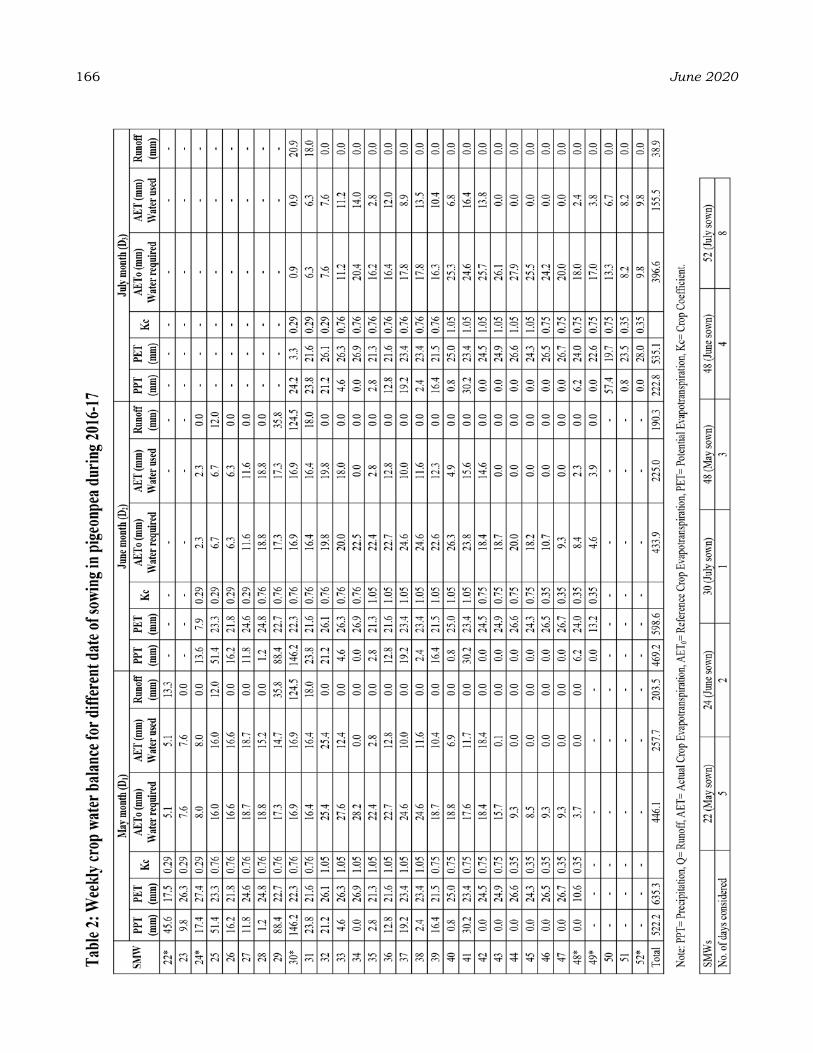
166 June 2020

168 June 2020

was more than the June (225.0 mm) and July (155.5 mm) sown crop.

On critical observation records of the different components of crop water balance, it is found that the runoff was drastically reduced in all the dates of sowing during both the years. Delayed sowing of pigeonpea viz., June and July month shows lower runoff, because of lower precipitation at reproductive stage of crop during both the years. Similarly, more is the water deficit in June and July sown pigeonpea. Hence, more reduction in pigeonpea growth and grain yield. These findings are similar with the findings of Tahshildar (2014) in pigeonpea and Guled et al. (2003) where in they have evaluated, cucumber (Cucumis melo) ridge gourd, sunflower, chickpea and rabi sorghum.

The grain yield and stalk yield of pigeonpea crop were significantly affected by row spacing (Table 3). The 60 cm row spacing shown significantly higher grain yield and stalk yield (940 and 4089 kg ha-1, respectively) followed by 90 cm row spacing (918 and 3059 kg ha-1, respectively) and significantly least grain and stalk yield was found with 120 cm spacing (731 and 2471 kg ha-1, respectively). The row spacing 60 cm to 90 cm had higher plant population (74, 074 to 49, 383 ha-1) per unit area. The higher plant population helps to get higher number of pods per unit area, which was resulted in higher grain yield of pigeonpea (Table 3). Similar findings were also reported by Pavan et al. (2011). Although, higher straw and grain yield was recorded with 60 cm row spacing but the improved yield and growth components was found with wider row spacing: 90 and 120 cm. It was mainly due to more spacing, higher moisture, light and nutrient availability in wider row spacing resulting in higher number of pods, weight of pods and grain weight / plant of pigeonpea crop.

Water use efficiencyThe WUE of pigeonpea varied significantly

with row spacing, varieties and date of sowing of pigeonpea crop during both the years of experiment and their pooled data (Table3). Among different row spacing, narrow row (60 cm) spacing showed significantly higher water use efficiency (1.79 kg ha-mm-1) compared to 120 cm row spacing (1.34 kg ha-mm-1). However, 90 cm row spacing (1.72 kg ha-mm-1) was similar with 60 cm. The higher water use efficiency in narrow row spacing was due to higher grain yield. The TTB-7 recorded significantly higher water use efficiency

(1.71 kg ha-mm-1) compared to BRG-2 (1.53 kg ha-mm-1). This might be due to TTB-7 resulted in higher grain and biomass accumulation yield of pigeonpea. Among different sowing date, May sown pigeonpea crop recorded significantly higher WUE (1.78 kg ha-mm-1) compared to June (1.62 kg ha-mm-1) and July (1.45 kg ha-mm-1) sown pigeonpea. This may be due to early sowing with longer growing period resulted in higher total biomass and grain yield.

Interaction of row spacing, varieties and sowing dates of pigeonpea shown significant difference with water use efficiency (Table 3). Significantly higher WUE (1.98 kg ha-mm-1) was observed in 60 cm row spacing with TTB-7 at May sown pigeonpea (S1V1D1) compared to other combinations. Significantly lower water use efficiency (0.97 kg ha-mm-1) was observed in 120 cm row spacing with BRG-2 variety at July sowing (S3V2D3). It was due to resulted in higher biomass acclamation and grain yield of pigeonpea. The results obtained in the present studies are in confirmation with the findings of Srivastava et al. (2008).

Among two years, 2015-16 recorded maximum rainfall and runoff and minimum potential evapotranspiration (PET) and actual evapotranspiration (AET) compared to 2016-17. It was indicated that 2015-16 favoures crop growth and development than 2016-17. The 2016-17 sown pigeonpea crops experienced more soil moisture during reproductive stage of the crop. Water deficit was recorded in June and July month pigeonpea crop sown at reproductive stage during 2015-16. Whereas, in 2016-17 all the dates of sown pigeonpea crop, soil moisture deficit was observed at reproductive stage of crop.

CoNCLuSIoNSOn critical examination of the different

components of crop water balance it was found that the runoff was drastically reduced in all the dates of sowing in both the year. Delay the sowing of pigeonpeaviz., June and July month lower runoff. Because low precipitation at reproductive stage of the crop in both years. Similarly, more water deficit in June and July sown pigeonpea. Hence, more drastic reduction in growth and grain yield of June and July sown pigeonpea.

reFereNCeSGomez, K. A. and Gomez, A. A., 1984, Statistical

Procedures for Agricultural Research. Second Edition. A Willey Inter-Science Publication, New York, USA, p. 693.

Guled, M. B., Lingappa, S., Itnal, C. J., Shirahatti, M. S. and Yaranal, R. S., 2003, Resource conversation and management in rainfed agro-ecosystem – A compendium far research and development. Techn. Bull., 34: 15-18.

Patel, N. R., Mehta, A. N. and Shekh, A. M., 2001, Canopy temperature and water stress quantificaiton in rainfedpigeonpea (Cajanuscajan (L.) Millsp.). Agril. Forest Met., 109: 223–232.

Pavan, A. S., Nagalikar, V. P., Pujari, B. T. and Halepyati, A. S., 2011, Influence of planting geometry on the growth characters, seed yield and economics of transplanted pigeonpea. Karnataka J. Agric. Sci., 24 (3) : 390 - 392.

Payero, J. O., Tarkalson, D. D., Irmak, S., Davison, D. and Petersen, J. L., 2008. Effect of irrigation amounts applied with subsurface drip irrigation on corn evapotranspiration, yield, water use efficiency, and dry matter production in a semi arid climate. Agric. Water Mngt., 95: 895–908.

Ratnam, M., Rajamani, S., Sreekanth, M. and Narayana, E., 2015, Crop weather

relationship in pigeonpea (CajanascajanL.). Int. J. App. and Pure Sci.1 (5) : 99-102.

Roder, W., Maniphone, S. and Keoboulapha, B. 1997. Pigeonpea for fallow improvement in slash-and-burn systems in the hills of Laos. Agrofore. Sys., 39 (1) : 45-57.

Sharma, A. and Guled, M. B. 2012. Effect of set-furrow method of cultivation in pigeonpea + greengram intercropping system in medium deep black soil under rainfed conditions. Karnataka J. Agril. Sci., 25 (1) : 22-24.

Srikrishnah, S. and Mahendran, S. 2007. The effects of soil moisture stress on the leaf water potential and yield of mungbean var. MI-6 at different growth stages. In: 63rd Ann. Sess. Proc. Sri Lanka Association for Advancement Science.

Srivastava, N. N., Rao, V. U. M., Ramakrishna, Y. S., Vijaya Kumar, P., and Subba Reddy, G., 2008, Studies on the radiation and water use efficiencies of medium duration pigeonpea (Cajanuscajan (L.) Millsp.) under different weather conditions. J. Agromet., (Spe issue - II) : 448-454.

Tahshildar, M. M., 2014, Planting geometry and nutrient requirement of pigeonpea under Zai method of cultivation in dryland situation. M. Sc. (Agri.) Thesis submitted to UAS, Dharwad.


thermal requirement for phenophases and yield of wheat varieties under various sowing environments and nitrogen levels in

sub-tropical region of Jammu

vIKaS guPta1*, MeeNaKShI guPta2, MaheNder SINgh3 aNd B. C. SharMa2

1Advance Centre for Rainfed Agriculture, Dhiansar, Samba-181133, 2Division of Agronomy, 3Agromet Research Center, SKUAST- Jammu, Chatha-180009

*corresponding author email: [email protected]

aBStraCtField experiments were conducted during rabi 2015-16 and 2016-17 at SKUAST-Jammu, Chatha Campus to study the influence of different sowing environments on phenology, thermal indices and yield of wheat varieties under sub tropical conditions of Jammu. The experiment was laid out in split split plot design with three wheat varieties (HD-2967, RSP-561 and WH-1105) in main plots, three sowing environments viz., 25th October (early), 14th November (normal) and 4th December (late) in sub plots and three levels of nitrogen (100, 125 and 150 kg N/ha) in sub sub plots replicated thrice. The results revealed that earlier sown wheat crop took more number of days (161) as compared to normal (149) and late sown (139) wheat crop and accumulated heat units 1769.8, 1636.1 and 1584.50C days, respectively for maturity along with numerically higher values of grain and straw yield as compared to the crop sown on 14th November and 4th December. However, accumulated helio thermal units (HTU) and photo thermal units (PTU) were 9539.8, 9059.1, 8511.10C days hour and 1916.4, 18289.2, 17638.7 0C days hour of wheat crop for physiological maturity sown under early, normal and late conditions, respectively. Among the varieties WH-1105 took maximum days (153) followed by HD-2967 (149) and RSP-561 (148) for acquiring physiological maturity. Varieties WH-1105, HD-2967 and RSP-561 consumed 1719.1, 1647.5 and 1623.80C days accumulated heat units (AHU) ; 9397.2, 8927.6, 8785.20C days hour accumulated helio-thermal units (AHTU) and 19050.9, 18137.2, 17846.20C days hour, accumulated photo-thermal units (APTU), respectively. Mean values of calendar days taken for physiological maturity were more (152) in higher dose of nitrogen (150 kg/ha) followed by numerical values 151 and 148 recorded in comparatively lower doses of nitrogen (125 and 100 kg/ha), respectively. Low mean temperature during early growth period resulted in longer vegetative phase in late sown crop.

Keywords: Sowing environments, varieties, nitrogen levels, heat units, heliothermal units, photothermal units

INtroduCtIoN

Wheat (Triticum aestivum L.) crop occupies an important position in agricultural sector and overall financial system especially in the Asian region. Its wide spread cultivation is due to its adaptation to different agro climatic conditions. It is one of the major sources of energy, protein and fibre in human diet (Arya et al., 2012). Wheat is the second most important cereal crop in the world after rice and globally cultivated on an area of 224.72 million ha with production and productivity of 734.62 million tonnes and 3.27 tonnes/ha, respectively (Anonymous, 2016).

India is one of the main wheat producing countries of the world after China. It is the second staple food crop of India, cultivated in about 30.60 million hectares with the production of

98.38 million tonnes and productivity of 32.16 q/ha (Anonymous, 2017). The major wheat growing states of India are Uttar Pradesh, Punjab, Haryana, Madhya Pradesh and Rajasthan. However, in Jammu and Kashmir state, it is grown both under irrigated as well as rainfed conditions on 0.32 mha with production and productivity of 0.50 million tonnes and 1550 kg/ha, respectively (Anonymous, 2016a).

Adequate growth and augmentation of crop could be obtained by adjusting the sowing environments which leads to better yield. Time of sowing plays an essential role in production of wheat crop; as perfect sowing environment exploits the full genetic potential of a particular variety by providing optimum growth conditions such as temperature, light, humidity and rainfall.


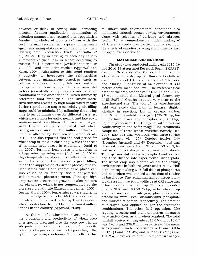
Advance or delay in sowing date, increasing nitrogen fertilizer application, optimization of irrigation management, reduced plant population density and choice of crop or cultivar with the best thermal requirement represent the main agronomic manipulations which help to maintain existing crop production levels (Ventralla et al., 2012). Delay in sowing by each day causes a remarkable yield loss in wheat according to various field experiments (Ortiz-Monasterio et al., 1994) and simulation models (Aggarwal and Kalra, 1994). Adaptation to this trend requires a capacity to investigate the relationships between crop management practices (such as cultivar selection, planting date and nutrient management) on one hand, and the environmental factors (essentially soil properties and weather conditions) on the another hand, which ultimately determine final crop yield. The unfavourable environments created by high temperature mostly during reproductive stages especially grain filling stage could be minimized by adjusting the sowing time to an optimum dates for different varieties, which are suitable for early, normal and late sown environmental conditions for assured higher yield. Current estimates indicated that wheat crop grown on around 13.5 million hectares in India is affected by heat stress (Sareen et al., 2012). It is also reported that the cool period for wheat crop in India is shrinking, while the threat of terminal heat stress is expanding (Joshi et al., 2007). Terminal heat stress is a problem in a large wheat growing area (Joshi et al., 2016). High temperatures, above 30oC, affect final grain weight by reducing the duration of grain filling, due to the suppression of current photosynthesis. Heat stress during the reproductive phase can also cause pollen sterility, tissue dehydration and increased photorespiration. Although high temperature accelerates growth, it also reduces the phenology, which is not compensated by the increased growth rate (Zahedi and Jenner, 2003). During March 2004, temperatures were higher in the Indo-Gangetic plains by 3-6oC and as a result, the wheat crop matured earlier by 10-20 days and wheat production dropped by more than 4 million tonnes in the country (Aggarwal, 2008).

As the role of sowing time is very crucial in the production and productivity of wheat crop in a specific area and also the crop sown in an adequate environment exploits the full genetic potential of a particular variety by providing it the optimum growing conditions. The ill effects due

to unfavourable environmental conditions also minimized through proper sowing environments along with selection of varieties and nitrogen levels. For a comprehensive understanding of all these, a study was carried out to swot out the effects of varieties, sowing environments and nitrogen levels on wheat.

MaterIaLS aNd MethodSThe study was conducted during rabi 2015-16

and 2016-17 at Agromet Research Farm, SKUAST-Jammu. Geographically, the experiment site is situated in the sub tropical Shiwalik foothills of Jammu region of J & K state at 32039/ N latitude and 74058/ E longitude at an elevation of 332 meters above mean sea level. The meteorological data for the crop seasons rabi 2015-16 and 2016-17 was obtained from Meterological observatory of SKUAST-J, Chatha situated very near to the experimental site. The soil of the experimental field was sandy clay loam in texture, slightly alkaline in reaction, low in organic carbon (0.38%) and available nitrogen (236.20 kg/ha) but medium in available phosphorus (13.10 kg/ha) and potassium (120.10 kg/ha) with electrical conductivity in the safer range. The treatments comprised of three wheat varieties namely HD-2967, RSP-561 and WH-1105, with three sowing environments viz., 25th October (early), 14th November (normal) and 4th December (late) and three nitrogen levels 100, 125 and 150 kg N/ha laid in split plot design with three replications. The experimental field was ploughed and levelled and then divided into experimental units/plots. The wheat crop was planted as per the sowing environments in both the years under study. Half of the nitrogen along with full dose of phosphorus and potassium was applied at the time of sowing as basal dose. The remaining half of nitrogen was top dressed in two equal splits i.e at CRI stage and before booting of wheat crop. The recommended dose of NPK was 100:50:25 kg/ha for wheat crop and the sources for nitrogen, phosphorus and potassium were urea, diammonium phosphate and muriate of potash, respectively. The amount of nitrogen was applied as per the treatment combinations. The other field operations like roguing, weeding and plant protection measures were undertaken, as and when required. The total rainfall received during rabi 2015-16 and 2016-17 was 148.8 and 238.0 mm respectively. The mean weekly maximum temperature varied from 13.0 to 36.10C (3 and 17 SMW) and 16.7 to 38.80C (3 and 16 SMW), however, minimum temperature ranged

Vol. 22, Special Issue GUPTA et al. 171

172 June 2020

from 2.5 to 17.30C (52 and 16 SMW) and 2.4 to 20.10C (2 and 16 SMW), during rabi 2015-16 and 2016-17 seasons, respectively (Fig. 1). Data was recorded for various crop phenological stages, grain yield, biological yield and harvest index. The growing degree days (GDD) or heat units (HU) were calculated by adopting the formula given by Nuttonson (1955) :

where, T max, Maximum temperature (0C) during a day; Tmin, Minimum temperature (0C) during a day; Tb, Base temperature (50C) for wheat crop under sub tropical conditions; a, Starting date of phenophase of interest, b, Ending date of phenophase of interest.

Photothermal unit (PTU) was calculated by multiplying GDD with maximum possible bright sunshine hours and expressed as 0C day hour. This was calculated using the formula Nuttonson (1956) :

Photo thermal units (PTU) = ΣGDD X maximum day length (0C day hrs)

Heliothermal unit (HTU) was calculated by multiplying GDD with bright sunshine hours and expressed as 0C day hour. This was calculated using the formula as given by Rajput (1980) :

Helio thermal units (HTU) = ΣGDD X bright (actual) sun shine hrs (0C day hrs)

The treatment-wise data recorded for different crop parameters were subjected to statistical analysis according to split split design as per the procedure outlined by Cochran and Cox (1963).

Fig. 1: Maximum and minimum temperatures during rabi 2015-16 and 2016-17

reSuLtS aNd dISCuSSIoNCrop phenology

Data pertaining to crop phenology, flowering (anthesis) and physiological maturity duration is presented in Table 1. Days taken to tillering were not much widely ranged due to different varieties, whereas a considerable difference in number of days taken to flag leaf, anthesis and physiological maturity was observed in various varieties. This

Table 1: Effect of different varieties, sowing environments and nitrogen levels on occurrence of various phenological stages (in days) of wheat crop (mean of 2 years)

treatments Phenology (in days) tillering Flag Leaf anthesis Physiological Maturity

varietiesV1: HD 2967 30 86 110 149V2: RSP 561 29 83 108 148V3: WH 1105 31 90 111 153Sowing environmentsD1: 25th October 27 83 114 161D2: 14th November 29 90 111 150D3: 4

th December 33 87 102 139Nitrogen levelsN1: 100 kg N/ha 29 84 108 148N2: 125 kg N/ha 30 87 110 151N3: 150 kg N/ha 31 89 111 152

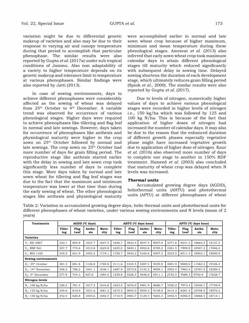
variation might be due to differential genetic makeup of varieties and also may be due to their response to varying air and canopy temperature during that period to accomplish that particular phenophase. The similar results were also reported by Gupta et al. (2017a) under sub tropical conditions of Jammu. Also non adaptability of a variety to higher temperature depends on its genetic makeup and tolerance limit to temperature at various phenophases. Similar findings were also reported by Jatti (2013).

In case of sowing environments, days to achieve different phenophases were considerably affected as the sowing of wheat was delayed from 25th October to 4th December. A variable trend was observed for occurrence of various phenological stages. Higher days were required to achieve phenophases like tillering and flag leaf in normal and late sowings. However, days taken for occurrence of phenophases like anthesis and physiological maturity were higher in the crop sown on 25th October followed by normal and late sowings. The crop sown on 25th October had more number of days for grain filling period. The reproductive stage like anthesis started earlier with the delay in sowing and late sown crop took significantly less number of days to complete this stage. More days taken by normal and late sown wheat for tillering and flag leaf stages was due to the fact that the maximum and minimum temperature was lower at that time than during the early sowing of wheat. The other phenological stages like anthesis and physiological maturity

were accomplished earlier in normal and late sown wheat crop because of higher maximum, minimum and mean temperature during these phenological stages. Amravat et al. (2013) also inferred that early sown wheat crop took maximum calendar days to attain different phenological stages till maturity which reduced significantly with subsequent delay in sowing time. Delayed sowing shortens the duration of each development stage, which ultimately reduces grain filling period (Spink et al., 2000). The similar results were also reported by Gupta et al. (2017).

Due to levels of nitrogen, numerically higher values of days to achieve various phenological stages were recorded in higher levels of nitrogen i.e., 150 kg/ha which was followed by 125 and 100 kg N/ha. This is because of the fact that application of higher doses of nitrogen had increased the number of calendar days. It may also be due to the reason that the enhanced duration of different growth phases especially vegetative phase might have increased vegetative growth due to application of higher dose of nitrogen. Kaur et al. (2016) also observed more number of days to complete one stage to another in 150% RDF treatment. Hameed et al. (2003) also concluded that maturity of wheat crop was delayed when N levels was increased.

Thermal unitsAccumulated growing degree days (AGDD),

heliothermal units (AHTU) and photothermal units (APTU) at different phenophases of wheat

Table 2: Variation in accumulated growing degree days, helio thermal units and photothermal units for different phenophases of wheat varieties, under various sowing environments and N levels (mean of 2 years)

treatments agdd (0C days) ahtu (0C days hour) aPtu (0C days hour)

tiller-ing

Flag Leaf

anthe-sis

Matu-rity

tiller-ing

Flag Leaf

anthe-sis

Matu-rity

tiller-ing

Flag Leaf

anthe-sis

Matu-rity

varieties

V1: HD 2967 332.1 804.8 1027.7 1647.5 1656.7 3832.4 5047.4 8927.6 3371.8 8231.2 10663.5 18137.2

V2: RSP 561 327.7 775.6 1013.8 1623.8 1653.0 3650.1 4952.6 8785.2 3361.5 7909.0 10507.2 17846.2

V3: WH 1105 345.5 831.9 1053.2 1719.1 1729.7 3942.2 5165.6 9397.2 3523.5 8511.4 10953.1 19050.9

Sowing environments

D1: 25th October 381.3 881.8 1126.0 1769.8 2111.6 4324.5 5387.4 9539.8 4001.9 9000.0 11563.3 19106.4

D2: 14th November 346.2 786.2 1041.1 1636.1 1687.9 3573.8 5132.3 9059.1 3502.4 7962.4 10767.5 18289.2

D3: 4th December 277.8 744.3 927.6 1584.5 1239.8 3526.4 4646.0 8511.1 2752.5 7689.3 9792.9 17638.7

Nitrogen levels

N1: 100 kg N/ha 328.2 781.4 1017.5 1616.8 1653.0 3676.0 4981.9 8686.7 3350.2 7973.4 10546.7 17749.9

N2: 125 kg N/ha 334.6 810.0 1031.6 1681.2 1675.5 3845.0 5054.3 9158.0 3414.3 8281.4 10708.5 18570.2

N3: 150 kg N/ha 342.4 820.8 1045.6 1692.4 1710.9 3903.7 5129.4 9265.3 3492.4 8396.9 10868.5 18714.1


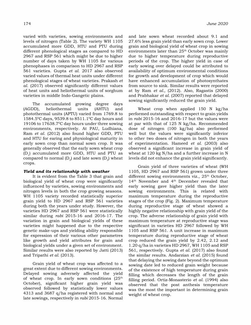
174 June 2020

varied with varieties, sowing environments and levels of nitrogen (Table 2). The variety WH 1105 accumulated more GDD, HTU and PTU during different phenological stages as compared to HD 2967 and RSP 561 which might be due to higher number of days taken by WH 1105 for various phenophases in comparison to HD 2967 and RSP 561 varieties. Gupta et al. 2017 also observed varied values of thermal heat units under different phenological stages of wheat varieties. Prakash et al. (2017) observed significantly different values of heat units and heliothermal units of sorghum varieties in middle Indo-Gangetic plains.

The accumulated growing degree days (AGDD), heliothermal units (AHTU) and photothermal units (APTU) varied from 1769.8 to 1584.50C days, 9539.8 to 8511.10C day hours and 19106 to 17638.70C day hours under three sowing environments, respectively. At PAU, Ludhiana, Ram et al. (2012) also found higher GDD, PTU and HTU for earing and physiological maturity in early sown crop than normal sown crop. It was generally observed that the early sown wheat crop (D1) accumulated more GDD, HTU and PTU as compared to normal (D2) and late sown (D3) wheat crops.

Yield and its relationship with weatherIt is evident from the Table 3 that grain and

biological yield of wheat crop were significantly influenced by varieties, sowing environments and nitrogen levels in both the crop growing seasons. WH 1105 variety recorded statistically superior grain yield to HD 2967 and RSP 561 varieties during both the years under study. However, the varieties HD 2967 and RSP 561 were statistically similar during rabi 2015-16 and 2016-17. The variation in grain and biological yields of these varieties might happened due to the respective genetic make-ups and yielding ability responsible for expression of their various other parametres like growth and yield attributes for grain and biological yields under a given set of environment. Similar results were also reported by Jatti (2013) and Tripathi et al. (2013).

Grain yield of wheat crop was affected to a great extent due to different sowing environments. Delayed sowing adversely affected the yield of wheat crop. In early sown conditions (25th October), significant higher grain yield was observed followed by statistically lower values 4313 and 3687 q/ha registered with normal and late sowings, respectively in rabi 2015-16. Normal

and late sown wheat recorded about 9.1 and 27.6% less grain yield than early sown crop. Lower grain and biological yield of wheat crop in sowing environments later than 25th October was mainly due to higher temperature during reproductive periods of the crop. The higher yield in case of early sowing over delayed could be attributed to availability of optimum environmental conditions for growth and development of crop which would have enhanced accumulation of photosynthates from source to sink. Similar results were reported at by Ram et al., (2012). Also, Ragastis (2000) and Prabhakar et al. (2007) reported that delayed sowing significantly reduced the grain yield.

Wheat crop when applied 150 N kg/ha performed outstanding with respect to grain yields in rabi 2015-16 and 2016-17 but the values were at par with that of 125 N kg/ha. Recommended dose of nitrogen (100 kg/ha) also performed well but the values were significantly inferior to other two doses of nitrogen in both the years of experimentation. Hameed et al. (2003) also observed a significant increase in grain yield of wheat at 120 kg N/ha and a further increase in N levels did not enhance the grain yield significantly.

Grain yield of three varieties of wheat (WH 1105, HD 2967 and RSP 561) grown under three different sowing environments viz., 25th October, 14th November and 4th December revealed that early sowing gave higher yield than the later sowing environments. This is related with maximum temperature during the reproductive stages of the crop (Fig. 2). Maximum temperature during reproductive stage of wheat showed a highly negative relationship with grain yield of the crop. The adverse relationship of grain yield with maximum temperature at reproductive stage was significant in varieties HD 2967 followed by WH 1105 and RSP 561. A unit increase in maximum temperature during reproductive stage of wheat crop reduced the grain yield by 2.42, 2.12 and 1.20 q/ha in varieties HD 2967, WH 1105 and RSP 561, respectively. Gupta et al. (2017) also found the similar results. Andarzian et al. (2015) found that delaying the sowing date beyond the optimum sowing date led to reduced grain weight because of the existence of high temperature during grain filling which decreases the length of the grain filling period. Ortiz-Monasterio et al. (1994) also observed that the post anthesis temperature was the most the important in determining grain weight of wheat crop.

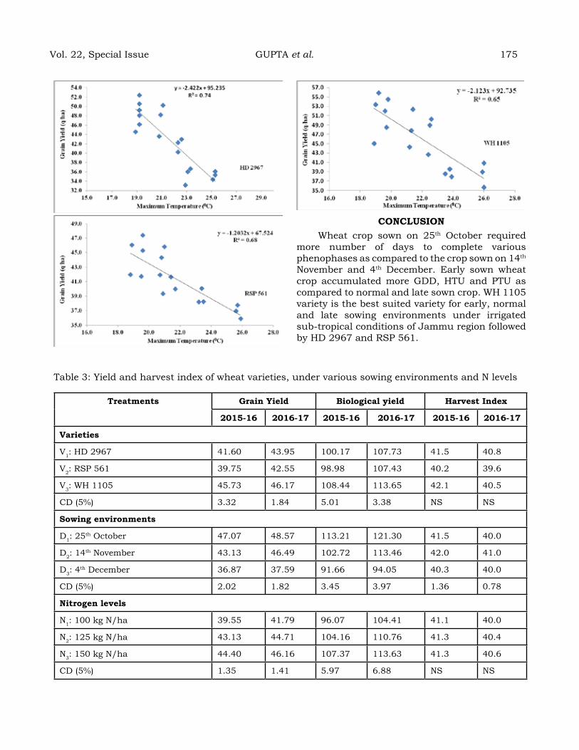
CoNCLuSIoNWheat crop sown on 25th October required

more number of days to complete various phenophases as compared to the crop sown on 14th November and 4th December. Early sown wheat crop accumulated more GDD, HTU and PTU as compared to normal and late sown crop. WH 1105 variety is the best suited variety for early, normal and late sowing environments under irrigated sub-tropical conditions of Jammu region followed by HD 2967 and RSP 561.

Table 3: Yield and harvest index of wheat varieties, under various sowing environments and N levels

treatments grain Yield Biological yield harvest Index

2015-16 2016-17 2015-16 2016-17 2015-16 2016-17

varieties

V1: HD 2967 41.60 43.95 100.17 107.73 41.5 40.8

V2: RSP 561 39.75 42.55 98.98 107.43 40.2 39.6

V3: WH 1105 45.73 46.17 108.44 113.65 42.1 40.5

CD (5%) 3.32 1.84 5.01 3.38 NS NS

Sowing environments

D1: 25th October 47.07 48.57 113.21 121.30 41.5 40.0

D2: 14th November 43.13 46.49 102.72 113.46 42.0 41.0

D3: 4th December 36.87 37.59 91.66 94.05 40.3 40.0

CD (5%) 2.02 1.82 3.45 3.97 1.36 0.78

Nitrogen levels

N1: 100 kg N/ha 39.55 41.79 96.07 104.41 41.1 40.0

N2: 125 kg N/ha 43.13 44.71 104.16 110.76 41.3 40.4

N3: 150 kg N/ha 44.40 46.16 107.37 113.63 41.3 40.6

CD (5%) 1.35 1.41 5.97 6.88 NS NS


176 June 2020

reFereNCeSAggarwal, P. K. (2008). Global climate change and

Indian Agriculture: Impacts, adaptation and mitigation. Indian J. Agric. Sci., 78 (10) : 911-919.

Aggarwal, P. K. and Kalra, N. (1994). Analysing the limitations set by climatic factors, genotype, water and nitrogen availability on productivity of wheat-II. Climatically potential yield and management strategies. Field Crops Res., 38: 93-103.

Amravat, T., Solanki, N. S., Sharma, S. K., Jajoria, D. J. and Dotaniya, M. L. (2013). Phenology, growth and yield of wheat in relation to agrometerological indices under different sowing dates. Afric. J. Agric. Res., 8: 6366-6374.

Andarzian, B., Hoogenboom, G., Bannayan, M., Shirali, M. and Andarzian, B. (2015). Determining optimum sowing date of wheat using CSMCERES-Wheat model. J. Saudi Soc. Agric. Sci., 14: 189-199.

Anonymous (2016). The Economic Survey of India. Department of Economics and Statistics, Government of India.

Anonymous (2016a). Agricultural Statistics at a glance. Government of India, Ministry of Agriculture and Farmers Welfare, Department of Agriculture, Cooperation and Farmers Welfare, Directorate of Economics and Statistics, New Delhi.

Anonymous (2017). Pocket Book of Agricultural Statistics. Government of India, Ministry of Agriculture and Farmers Welfare, Department of Agriculture, Cooperation and Farmers Welfare, Directorate of Economics and Statistics, New Delhi.

Arya, R. K., Munjal, R. and Dhanda, S. S. (2012). Evaluation of bread, durum and synthetic wheat and triticale for physiological traits under heat stress conditions. In: National Seminar on Sustainable Agriculture and Food Security: challenges in changing climate, March 27-28, 2012 at CCSHAU, Hisar.

Cochran, G. and Cox, G. M. (1963). Experimental design. Asia Publishing House, Bombay, India.

Gupta, M., Sharma, C., Sharma, R., Gupta, V. and Khushu, M. K. (2017). Effect of sowing time on productivity and thermal utilization of mustard (Brassica juncea) under sub-

tropical irrigated conditions of Jammu J. Agrometeorol., 19 (2) : 137-141.

Gupta, M., Sharma, C., Sharma, B. C. and Singh, M. (2017a). Influence of weather conditions on phenology, thermal indices and yield of wheat cultivars under sub-tropical conditions of Jammu. J. Agrometeorol., (Special Issue-AGMET 2016) 19: 92-97.

Hameed, E., Shah, W. A., Shad, A. A., Bakht, J. and Muhammad, T. (2003). Effect of different planting dates, seed rate and nitrogen levels on wheat. Asian J. Plant Sci., 2 (6) : 467-474.

Jatti, R. (2013). Effect of sowing dates on microclimate, growth and yield of wheat varieties. M.Sc. Thesis, Department of Agronomy, COA, UAS, Dharwad-580005.

Joshi, A. K., Mishra, B., Chatrath, R., Ortiz Ferrara, G. and Singh, R. P. (2007). Wheat improvement in India: present status, emerging challenges and future prospects. Euphytica, 157: 431-446.

Joshi, M. A., Faridullah, S. and Kumar, A. (2016). Effect of heat stress on crop phenology, yield and seed quality attributes of wheat (Triticum aestivum L.). J. Agrometeorol., 18 (2) : 206-215.

Kaur, H., Ram, H., Sikka, R. and Kaur, H. 2016. Productivity, agronomic efficiency and quality of bread wheat (Triticum aestivum L.) cultivars in relation to nitrogen. Inter. J. Agric. Environ. Biotechnol., 9 (1) : 101-106.

Nuttonson, M. Y. (1955). Wheat-climate relationships and the use of phenology in ascertaining the thermal and photothermal requirements of wheat. American Institute of crop Ecology, Washington D.C.: 388.

Nuttonson, M. Y. (1956). A comparative study of lower and upper limits of temperature in measuring variability of day-degree summation of wheat, barley and rye. American Institute of Crop Ecology, Washington D.C.

Ortiz-Monasterio, J. I., Dhillon, S. S. and Fischer, R. A. (1994). Date of sowing effects on grain yield and yield components of irrigated spring wheat cultivars and relationships with radiation and temperature in Ludhiana, India. Field Crops Res., 37 (3) : 169-184.

Prabhakar, B. N., Halepyati, A. S., Desai, B. K. and Pujari, B. T. (2007). Growing degree days and photothermal units accumulation

of wheat genotypes as influenced by dates off sowing. Karnat. J. Agric. Sci., 20 (3) : 594-595.

Prakash, V., Mishra, J. S., Kumar, R., Kumar, R. K., Kumar, S., Dwivedi, S. K., Rao, K. K. and Bhatt, B. P. (2017). Thermal utilization and heat use efficiency of sorghum cultivars in middle Indo-Gangetic Plains. J. Agrometeorol., 19 (1) : 29-33.

Ragastis, I. 2000. Effect of sowing dates on grain yield and quality of winter wheat. Novenyter Meles., 49 (6) : 641-649.

Rajput, R. P. (1980). Response of soybean crop to climatic and soil environments. Ph.D. Thesis, IARI, New Delhi, India.

Ram, H., Singh, G., Mavi, G. S. and Sohu, V. S. (2012). Accumulated heat unit requirement and yield of irrigated wheat (Triticum aestivum L.) varieties under different crop growing environment in central Punjab. J. Agrometeorol., 14 (2) : 147-153.

Sareen, S., Munjal, R., Singh, N. B., Singh, B. N., Varma, R. S., Meena, B. K., Shoran, J., Sarial, A. K. and Singh, S. S. (2012).

Genotype X environment interaction and AMMI analysis for heat tolerance in wheat. Cereal Res. Commun., 40 (2) : 267-276.

Spink, J. H., Semere, T., Sparkes, D. L., Wahley, J. M., Foulkes, M. J., Calre, R. W. and Scatt, R. K. (2000). Effect of sowing dates and planting density of winter wheat. Annals of Appl. Biol., 137 (2) : 179-188.

Tripathi, N. 2003. Studies on physiological parameters in relation to heat tolerance in eight wheat varieties. M. Sc. (Agronomy) Thesis, GBPUAT, Pantnagar, Uttaranchal.

Ventrella, D., Charfeddine, M., Gigilo, L. and Castellini, M. (2012). Application of DSSAT models for an agronomic adaptation strategy under climate change in Southern Italy: optimum sowing and transplanting time for winter durum wheat and tomato. Italian J. Agron., 7 (16) : 109-115.

Zahedi, M. and Jenner, C. F. (2003). Analysis of effects in wheat of high temperatures on grain filling attributes estimated from mathematical models of grain filling. J. Agric. Sci., 141: 203-212.


reSPoNSe oF Wheat geNotYPeS to dIFFereNt SoWINg tIMeS IN reLatIoN to therMaL eNvIroNMeNtS IN harYaNa

Bhagat SINgh*, MuKeSh KuMar, a.K. dhaKa aNd raJ SINgh1

Department of Agronomy, CCS Haryana Agricultural University, Hisar-125004, India1Department of Agrometeorology, CCS Haryana Agricultural University, Hisar-125004, India

*Correspondence e-mail: [email protected]

aBStraCtField study was carried out during the Rabi season of 2017-18 and 2018-19 at CCS Haryana Agricultural University, Hisar (Lat. 29°10’ N, Log. 75°46’ E and 215.2 m amsl) to investigate the effect of different environments on wheat genotypes. The experiment was laid out in split plot design with three sowing dates viz. 5th November, 15th December and 5th January in main plot and eight genotypes of wheat viz. HD 3226, HD 3059, DBW 71, DBW 173, PBW 752, HD 3086, PBW 757 and WR 544 in subplots, replicated thrice. On the basis of two years pooled data, it was revealed that wheat crop sown on 5th November took maximum calendar days (147.58 days), GDD (1805 0C day), HTU (100820 days hour), PTU (199660 days hour), Tp (3051.10C) and Tn (1832.8 0C) upto physiological maturity, which reduced significantly under15th December and 5th January sowings. Yield attributes and grain yield were also higherin 5th November sowing, which were significantly higher as compared to 15th December and 5th January sowings. Crop sown on 5th November possess highest grain yield (58.72 q/ha), which was significantly higher than 15th December (47.29 q/ha) and 5th January sown crop (40.06 q/ha), mainly due to maximum number of effective tillers/m2 (427.71), grains/earhead (49.51) and 1000 grain weight (41.55g) in 5th November sown crop. The reduction in grain yield was 19.47 and 31.78 percent by delayed sowing on 15th December and 5th January, respectively as compared to 5th November sowing. Among different genotypes, HD 3226 took maximum days to maturity (124 days) and GDD (1605.8 oC days). However, PBW 752 produced significantly higher grain yield (52.71 q/ha) as compared to other genotypes except HD 3086 (51.96 q/ha) and DBW 173 (51.06 q/ha), which was mainly due to maximum number of effective tillers/m2 in PBW 752 (419.5). Whereas, minimum grain yield (39.66 q/ha) was recorded in WR 544. The grain yield and biological yield were highly correlated with the accumulated GDD (0.89**, 0.93**), PTU (0.90**, 0.94**), HTU (0.81**, 0.87**) Tp (0.93**, 0.97**) and Tn (0.92**, 0.95**) clearly suggesting thereby the significant effect of these indices on the wheat crop.

Keywords: Wheat, Grain yield, Genotypes, Growing environment, Thermal indices

INtroduCtIoN

Wheat is the second most important cereal crop next to rice in Asia. In India, the crop occupies an area of about 29.55 mha with total production of 101.20 mt and a productivity of 3424 kg ha-1 during 2018-19. There are considerable yield gaps between the major wheat growing states in the country with highest yield recorded in Punjab (5077 kg/ha), followed by Haryana (4643 kg/ha) and lowest in Maharashtra with productivity of 1275 kg/ha (ICAR-IIWBR, 2019). Majority of the wheat area in Indo-gangetic plains falls under timely sown irrigated crop conditions. However, a sizeable area comes under late sown mainly in cropping systems such as rice-wheat, sugarcane-wheat, potato-wheat, vegetable pea-wheat, etc. In these cropping systems, late harvest of preceding crops resulted in delay sowing of wheat. Among production factors, sowing time and varieties

selection are the most crucial factors deciding the productivity. For timely sown crop long duration varieties are suitable but under late sown conditions short duration varieties perform better because they complete their lifecycle in shorter period and escape terminal heat. Late sown wheat faces low temperature in the earlier part and high temperature stress in the later part of the growing season (Alam et al., 2013). Under late sowing of wheat, anthesis and grain filling period faces increased temperature (more than 20°C) resulted in low yield. Yield of wheat is much affected by relatively short periods (3-5 days) of heat stress, especially when crop coincides with reproductive phase of grain filling stage (Farooq et al., 2011). Delay in sowing of wheat beyond 15th December, resulted in yield reduction of 50 kg grain/day/ha (Singh et al., 2001). Adopting suitable sowing date and appropriate cultivar choices were estimated to be avoiding 7-18% of global yield


losses due to changed scenarios of temperature and precipitation in 2050s (Deryng et al., 2011).

Temperature based indices such as growing degree-days (GDD), helio-thermal unit (HTU), photo-thermal unit (PTU), pheno-thermal index (PTI) can be relatively useful for predicting growth and yield of crop. Plants have a definite temperature requirement to accomplish phenological stages. Because of close relation between temperature and plant development, GDD are frequently used as an indicator for crop development evaluation. Therefore, it’s currently important to have exact information of the phonological stages duration and their related effect on grain yield. The quantification of HUE is useful for the assessment of yield potential of a crop in different environment. So, the present study was carried out to study the performance of newly evolved cultivars under different sowing times to identify the best-suited cultivar for Haryana conditions.

MaterIaLS aNd MethodS The field experiment was conducted at

Research Farm of CCS Haryana Agricultural University, Hisar, India (29º10’N latitude, 75º46’E longitude and 215.2 M altitude) during Rabi season of 2017-18 and 2018-19. The soil of the field was sandy loam in texture, slightly alkaline in pH (7.9), low in organic carbon, poor in available nitrogen and medium in available phosphorus and available potassium. The experiment was laid out in split plot design with three sowing dates (5th November, 15th December and 5th January) in main plot and eight genotypes (HD 3226, HD 3059, DBW 71, DBW 173, PBW 752, HD 3086, PBW 757 and WR 544) in sub plots with three replications. The crop was sown on 20 cm row spacing with seed rate of 100 kg/ha. Full dose of P2O5 (62.5 kg/ha) and 1/3rd dose of nitrogen (50 kg/ha) was applied basal at the time of sowing. The remaining 2/3rd dose of nitrogen was applied in to two equal dosesi.e. half at CRI stage and the rest half at tillering stage. One hand weeding was done at 30 days after sowing to control the weeds. Other management practices were adopted as per recommendations of the wheat crop under irrigated condition. During 2017-18, 5th November, 15th December and 5th January sown crop were harvested on 14th, 18th and 27th April, 2018, respectively, while in 2018-19, 5th November, 15th December and 5th January sown crop were harvested on 17th, 22nd and 28th April, 2019, respectively. During crop season the meteorological data, viz., rainfall,

relative humidity, maximum (Tmax) and minimum temperature (Tmin), bright sunshine hours (BSS) and pan evaporation etc. were recorded from Agrometeorological observatory, CCS HAU, Hisar. The agro-meteorological indices were computed using the daily meteorological data. The dates of occurrences of different phenological events, viz. 50% heading and physiological maturity were recorded when 50 percent of the plants in each replication reached the respective stages.

The different temperature based meteorological indices such as growing degree days (GDD), helio-thermal unit (HTU), photo-thermal unit (PTU), pheno-thermal index (PTI) and heat use efficiency (HUE) were calculated using the standard formulae (Gill et al., 2014). Phototemperature (Tp) and nyctotemperature (Tn) measured with the help of formula given by Dalezios et al. (2002).

reSuLtS aNd dISCuSSIoNWeather conditions during wheat growing period (2017-18 and 2018-19)

Weekly Tmax and Tmin ranges were 16.9-37.6oC and 2.6-19.4oC during 2017-18 and 17.1-36.9oC and 1.9-20.0oC, respectively during 2018-19 (Fig. 1). During crop season highest (37.6 oC) and lowest (16.9oC) weekly mean Tmax was recorded in 16th & 50th SMWs, respectively during 2017-18 and 36.9 oC and 17.1 oC in 15th and 5th SMWs during 2018-19. Whereas, weekly mean Tmin, the highest (19.4oC) and lowest (2.6oC) were recorded in 16th & 2nd SMWs, respectively during 2017-18 and 20.0oC and 1.9oC were recorded in 15th and 52nd SMWs, respectively during 2018-19. The rainfall of 3.8, 10.9, 1.2 and 14.0 mm was received in 50th, 4th, 7th and 14th SMWs during the crop season of 2017-18, whereas, only 14.8 and 8.2 mm of rainfall was received during the 9th and 16th SMW of 2018-19 crop seasons.

Fig. 1: Weather conditions prevailed during 2017-18 and 2018-19


180 June 2020

Plant height: Plant height decreased significantly with delay in sowing (Table 1) and tallest plant (106.25 cm) was recorded under 5th November sown crop which was significantly higher than 15th December (95.29cm) and 5th January sown crop (89.75cm). Among genotypes, WR 544 recorded significantly taller plants as compared to all other genotypes.

Yield attributesEffective tillers/m2: Effective tillers/ m2

decreased significantly by delayed sowing of wheat (Table 1). On mean basis, maximum number of effective tillers/m2 (427.7) were recorded in 5th November sown crop, which were significantly higher as compared to 15th December (407.7) and 5th January (351.6) sown crop. The reduction in effective tillers/m2 was 4.68 and 17.8 percent due to delayed sowing on 15th December and 5th January, respectively as compared to 5th November sown crop. Singh and Dwivedi (2015) also recorded reduction in effective tillers/m2 with delay in sowing. This might be due to favourable temperature as per crop need which boosted crop growth in the form of higher photosynthate accumulation and resulting in higher yield

parameters in normal sown crop than late sown (Elrahman et al., 2014). Among genotypes on pooled mean basis, the maximum number of effective tillers/m2 (419.5) was recorded with PBW 752, which was significantly higher than other genotypes except HD 3086 (408.3). Whereas, minimum numbers of effective tillers (368.9) were recorded in WR 544. Differences in number of effective tillers among genotypes might be due to their genetic diversity (Mumtaj et al., 2015).

Grains/ear head: Pooled means of two years indicated that numbers of grains/ear head were also decreased with delayed sowing. Grains/ear head were significantly higher in 5th November sown crop as compared to 15th December and 5th January sowings. The reduction in grains/ear head was 6.77 and 13.05 percent due to delayed sowing on 15th December and 5th January, respectively as compared to 5th November sown crop. Singh et al. (2018) and Kumar et al. (2018) also reported decrease in grains/ear head under delayed sowings. Among genotypes, maximum number of grains/ear head (50.01) were recorded in DBW 173, which were significantly higher as compared to other genotypes in the study except

Table:1Effect of date of sowing on yield attributes, yields (q/ha) and quality of different wheat genotypes (pooled mean of 2017-18 and 2018-19 )

treatments Plant height (cm)

effective tillers/

m2

grains/ earhead

1000 grain

weight (g)

grain yield (q/ha)

Straw Yield (q/ha)

Biologi-cal Yield (q/ha)

har-vest

Index

Hec-toliter weight

(kg/hl) )

Sedimen-tation

value (ml)

Sowing time

Timely (5th November)

106.25 427.7 49.51 41.55 58.72 97.85 156.57 37.54 80.71 40.04

Late (15th December)

95.29 407.7 46.16 38.06 47.29 77.25 124.54 37.99 78.28 41.33

Very Late (05th January)

89.75 351.6 43.05 35.75 40.06 62.81 102.87 38.98 77.67 42.33

S. Em± 0.29 3.9 0.31 0.21 0.52 0.99 1.49 0.10 0.19 1.11

LSD (P=0.05) 1.16 15.7 1.23 0.86 2.08 4.00 6.03 0.41 0.77 NS

genotypes

HD 3226 102.22 388.6 46.42 37.27 46.31 86.74 133.05 35.00 78.32 50.89

HD 3059 96.94 389.5 46.14 38.14 49.88 84.20 134.08 37.34 78.49 40.89

DBW 71 95.78 399.5 44.27 37.96 48.13 73.81 121.94 39.82 80.46 36.00

DBW 173 99.33 398.9 50.01 37.82 51.06 84.19 135.24 37.89 76.68 40.33

PBW 752 95.72 419.5 47.19 40.05 52.71 85.80 138.51 38.09 78.47 44.67

HD 3086 96.83 408.3 46.82 40.15 51.96 80.91 132.86 39.10 80.78 38.78

PBW 757 84.39 392.2 48.98 37.30 49.83 70.82 120.64 41.35 79.94 38.56

WR 544 105.56 368.9 40.09 38.93 39.66 67.95 107.62 36.76 77.95 39.78

S. Em± 0.56 6.3 0.40 0.27 0.67 1.00 1.55 0.21 0.29 1.51

LSD (P=0.05) 1.61 18.1 1.15 0.78 1.91 2.87 4.45 0.61 0.84 4.32

PBW 757.

1000 grain weight: Data revealed that 1000 grain weight decreased significantly by delayed sowing and bolder grains were recorded in 5th November sown crop as compared to 15th December and 5th January sown crop. The reduction in 1000-grain weight was 8.40 and 13.96 percent due to delayed sowing on 15th December and 5th January, respectively as compared to timely sown crop (5th November). The reduction in 1000-grain weight under late sowing was mainly due to shorter growth period resulted in less production of photosynthateand due to winds prevailed during milk and grain filling stage resulted inshriveling of grains. These results are in line with those of Singh et al. (2018) and Singh and Dwivedi (2015).

Among the genotypes, the maximum 1000 grain weight (40.15) was recorded with HD 3086, which was significantly higher than other genotypes except PBW 752 (40.05). Differences in 1000 grains weight of wheat cultivars seem to be due to their genotypic variations (Mahmood et al., 2014).

Grain, Straw and Biological yield and Harvest index

Pooled data of two experimental years revealed that highest grain yield (58.72 q/ha), straw yield (97.85 q/ha) and biological yield (156.57 q/ha) were recorded under 5th November sowing, which were significantly higher than delayed sowing on 15th December and 5th January. The reduction in grain yield was 19.47 and 31.78 percent by delayed sowing on 15th December and 5th January, respectively as compared to 5th November sowing (Table 1). It might be due to higher yield attributes viz. effective tillers/m2, grains/ear head and 1000 grain weight recorded in 5th November sowing (Table 1). The detrimental effect of heat at later stage of crop development and ear head emergence in very late sowing was adversely effected the grain yield. In late planted wheat, time to heading shortens in a curvilinear fashion as temperature increases and grain development period also reduced and crop matures early. Harvest index was higher in very late sown crop. Among wheat genotypes, PBW 752 recorded the highest grain yield (52.71 q/ha) which was significantly higher than other genotypes except HD 3086 (51.96 q/ha) and DBW 173 (51.06 q/ha) which were statistically at par with PBW 752. Highest grain yield in genotype PBW 752 mainly due to maximum number of effective tillers/m2

(419.45) and second highest 1000 grain weight (40.05). Yield variation among different genotypes might be due difference in their genetic potential. The highest straw yield (86.74 q/ha) was recorded in HD 3226, which was significantly higher than other genotypes except PBW 752 and DBW 173. The highest biological yield (138.51 q/ha) was also recorded with PBW 752, which was significantly higher than other genotypes except DBW 173 and HD 3059. It might be due to maximum number of effective tillers in PBW 752. Varietal change had significantly affected the harvest index and PBW 757 was recorded with highest harvest index (41.35%), which was significantly higher than all genotypes.

The greater reduction in grain yield of wheat genotypes under delayed sowing situations was mainly due to decrease in season length, which might have reduced their yield. Delayed sowing hastened the crop phenological development, thereby causing significant reduction in yield attributes and wheat yields. Elrahman et al. (2014) also reported the similar observation under delayed sowing. Singh et al. (2018) also recorded higher grain yield in timely planting wheat mainly due to increased higher growing degree days, photo-thermal units and yield attributes.

Sedimentation value and Hectolitre weight: Significantly higher hectolitre weight (HW) value (80.71 kg/hl) was recorded in 5th November sowing as compared to 15th December and 5th January sowings. The highest hectolitre weight in timely sown crop might be due to favourable prevailing temperature conditions. The decline in hectolitre weight in late and very late sowing might be due to very high temperature at reproductive stage, thus subjecting to forced maturity and drying of immature seeds at the time of grain filling, led to reduction in grain size and poor density and thereby lower HW (Meena et al., 2016). The delay in sowing led to increase in sedimentation value (42.33 ml), however the difference was non-significant. Among genotypes, maximum hectolitre weight (80.78 kg/hl) was observed in HD 3086 and maximum sedimentation value in HD 3226 (50.89 ml).

Days taken to phenophases: Sowing times and genotypes had significantly affected the days taken to different phenophases viz. 50% heading and physiological maturity (Table 2). The crop sown on 5th November took maximum number of days upto 50% heading (99.46) and


182 June 2020

physiological maturity (147.58), which were 11.83 and 32.70 days higher than late (15th December) and 22.58 and 47.95 days than very late sowing on 5th January, respectively. The late sown crop completed its life cycle at an accelerated pace, leading to shortening of days taken for the development of its different phenophases up to maturity. In late planted wheat, time to heading shortens in a curvilinear fashion as temperature increases and grain development period is reduced and crop matures early (Mumtaj et al., 2015). Among genotypes, HD 3226 and WR 544 took the maximum and minimum days, respectively for all the phenophases upto maturity. Elrahman et al. (2014) also reported the significant differences among the genotypes with respect to the number

of days to phenophases indicate that each of genotype has its own genetic characteristics with respect to this trait.

Growing degree days (GDD) :Accumulated growing degree days upto different phenophasis were recorded with significant difference under different sowing times and genotypes (Table 2). Wheat crop sown on 5th November was recorded with 9.63 and 20.21 percent higher GDD over late and 10.12 and 23.20 over very late sowing up to 50% heading and maturity, respectively over 5th November sown crop. Pandey et al. (2010) also reported lower consumption of heat units under delayed sowing. The requirement of GDD was higher for 15th December sowing than the 5th

Table 2: Effect of sowing time and varieties on days taken and accumulated growing degree days (GDD), Heliothermal units (HTU), Photothermal units (PTU) and pheno-thermal index (PTI) for 50% heading and Physiological Maturity of wheat.

Treat-ments

Days taken to

GDD (0C day) HTU (0days hour) PTU (0days hour) PTI (0C days day-1)

Tp (°C) Tn (°C) GY HUE (kg ha-1 day-1)

BY HUE (kg ha-1 day-1)

50% H*

PM** 50% H PM 50% H PM 50% H PM 50% H PM 50% H PM 50% H PM

Sowing time

Timely (5th

Novem-ber)

99.46 147.58 1015.1 1805.0 4880.0 10082.9 10979.1 19966.0 10.21 12.24 1858.8 3051.1 1065.6 1832.8 3.26 8.68

Late (15th Decem-ber)

87.63 114.88 917.3 1440.1 5772.1 9285.5 10217.1 16583.2 10.45 12.53 1688.9 2458.5 950.7 1473.5 3.28 8.64

Very Late (05th Janu-ary)

76.88 99.63 912.3 1386.1 5911.3 9072.0 10382.3 16232.1 11.86 13.91 1583.2 2256.5 935.6 1414.0 2.89 7.41

S. Em± 0.41 0.33 6.81 6.26 46.33 43.44 89.52 84.28 0.02 0.02 9.41 10.04 7.14 7.25 0.02 0.07

LSD (P=0.05)

1.67 1.34 24.46 25.24 186.80 175.14 360.92 339.78 0.10 0.06 37.92 40.48 28.81 29.22 0.09 0.26

Genotypes

HD 3226

93.11 124.00 1021.7 1605.8 6027.0 10002.3 11391.0 18466.5 11.06 13.08 1827.0 2688.3 1058.7 1645.1 2.87 8.23

HD 3059

90.00 122.78 979.6 1580.1 5725.8 9773.6 10901.2 18144.8 10.96 12.98 1755.0 2652.6 1015.9 1619.1 3.15 8.45

DBW 71 87.11 118.78 931.3 1490.9 5417.6 9136.0 10349.2 17040.1 10.76 12.67 1684.2 2529.1 967.0 1528.8 3.22 8.12

DBW 173

91.00 122.78 990.8 1579.9 5803.2 9804.3 11026.3 18142.6 10.96 12.99 1777.8 2651.0 1027.7 1618.8 3.22 8.51

PBW 752

90.22 122.67 977.4 1578.3 5705.3 9824.4 10871.7 18122.8 10.91 12.98 1758.0 2649.9 1014.7 1620.2 3.34 8.76

HD 3086

88.33 121.56 951.3 1552.2 5519.6 9606.9 10553.6 17795.7 10.84 12.88 1714.1 2614.0 986.9 1590.4 3.33 8.53

PBW 757

87.00 119.11 929.0 1500.8 5393.8 9200.6 10283.0 17160.5 10.75 12.71 1698.3 2541.3 962.1 1539.0 3.30 7.99

WR 544 77.11 113.89 804.4 1462.0 4576.8 8492.8 8833.2 15877.4 10.46 12.83 1467.9 2383.2 838.8 1426.1 2.70 7.34

S. Em± 0.48 0.57 7.93 12.69 56.37 88.05 93.81 156.18 0.03 0.05 13.05 17.56 7.73 12.98 0.05 0.11

LSD (P=0.05)

1.38 1.62 22.70 36.35 161.45 252.19 268.67 447.32 0.09 0.15 37.39 50.29 22.15 37.18 0.15 0.33

January sowing. This was due to longer period for all the phenological stages in the 15th December sowing than 5th January sown conditions. Late sowing of wheat on 5th January recorded with lower duration of phenophases as compared to 15th December due to fluctuated unfavourable high temperature during the growing period. So, the requirement of heat units decreased for different phenological stages with late sowing. Similar results were also reported by Kumar and Kumar (2014). The maximum (1021.7) and minimum (804.0) GDD upto heading were acquired by HD 3226 and WR 544, respectively. For maturity, the maximum GDD was also reported with HD 3226 (1605.8) which was statistically at par with HD 3059 (1580.1), DBW 173 (1579.9) and PBW 752 (1578.3). The less number of days taken by WR 544 for development of various phenophases could be a reason for its significantly minimum GDD values. Strong positive relationship was also observed which signifies the importance of temperature based agrometeorological indices.

Helio-thermal unit (HTU) : Wheat crop sown on 5th November consumed higher HTU at maturity as compared to 15th December and 5th January sown crop (Table 2). This might be due to 32.7 and 47.95 more days taken up to maturity in timely sown crop (5th November) as compared to 15th December and 5th January sown crop. HTU for different phenological stages due to delayed sowing were also reported by Haidar et al. (2003) in wheat. Among different genotypes maximum accumulated HTU upto 50% heading and maturity was found with HD 3226 (6027.0 and 10002.3 0day hour, respectively), which was significantly higher than all other genotypes at 50% heading, however it was statistically at par with HD 3059 (9773.6), DBW 173 (9804.3) and PBW 752 (9824.4) at maturity.

Photo-thermal unit (PTU) : The data presented in Table 2 revealed that crop sown on 5th November used higher PTU by 6.94 and 20.40 per cent over 15th December and 5.43 and 18.70 per cent over 5th January sowing for heading and maturity, respectively. Among genotypes, HD 3226 was observed with highest PTU consumed for different phenophases, while lower PTU used for heading and maturity were found with WR 544 (8833.2 and 15877.4, respectively). The higher PTU value in early sown crop may be due to fact that crop took longer duration to reach phenological stages (Amrawat et al., 2013).

Pheno-thermal index (PTI) : Pheno-thermal index was higher at maturity than at 50% heading (Table 2). Highest PTI value were observed in 5th January sown crop which was 11.88 and 9.92 per cent more than 15th December and 13.91 and 12 percent more over 5th November sown wheatupto 50% heading and maturity, respectively. Among different genotypes, maximum PTI values of 11.06 and 13.08 during 50% heading and physiological maturity, respectively were found with HD 3226 and these were statistically at par with HD 3059, DBW 173 and PBW 752 at physiological maturity. It might be due to variation in number of days taken during different phenophases. It was observed that the heat tolerant cultivar HD 3226 had the highest PTI at heading to maturity stage of different growing condition. Similar findings have been observed by Sikder (2009).

Grain and Biological Heat Use Efficiency (GY HUE and BY HUE)

Crop sown on 5th November and 15th

December showed significantly higher HUE of 3.26 and 3.28 kg ha-1 day-1 for grain yield and 8.68 and 8.64 kg ha-1 day-1 for biological yield, respectively than 5th January sown crop (Table 2). The HUE was decreased significantly with delay in sowing. Delayed sowing led to significant drop of HUE due to decreased biomass production and shortening of crop growing period resulting in lesser accumulation of HU. Similar findings were also reported by Sikder (2009) ; Amrawat et al. (2013) ; Kumar and Kumar (2014). In contrast, high temperature and water deficiency hampered normal metabolic activities resulted in lower grain yield as well as HUE in late sown crop (Haider et al., 2003). Among the genotypes, PBW 752 was recorded with maxi mum grain yield heat use efficiency (3.34 kg ha-1 day-1) and biological yield heat use efficiency (8.76 kg ha-1day-1). The higher value of HUE in PBW 752 might be attributed to their respective higher grain and biological yields. These findings are in confirmation with Singh and Khushu (2012).

Photo temperature (Tp) : The photo temperature was significantly influenced by different sowing dates (Table 2). The photo temperature was significantly higher in the timely sown (1858.8 and 3051.1 0C) than 15th December (1688.9 and 2458.5 0C) conditions and 5th January sown crop (1583.2 and 2256.5 0C) up to 50% heading and physiological maturity, respectively. Patra et al. (2016) also recorded that Tp decreased with delay sowing of wheat crop.


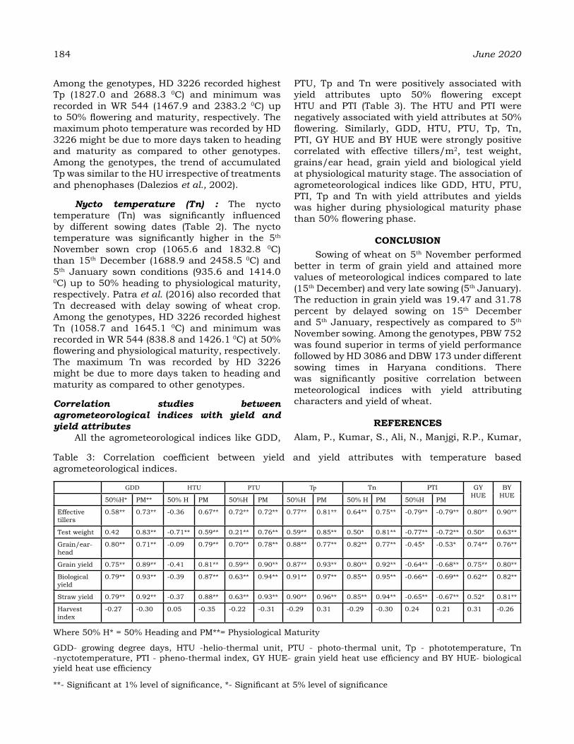
184 June 2020

Among the genotypes, HD 3226 recorded highest Tp (1827.0 and 2688.3 0C) and minimum was recorded in WR 544 (1467.9 and 2383.2 0C) up to 50% flowering and maturity, respectively. The maximum photo temperature was recorded by HD 3226 might be due to more days taken to heading and maturity as compared to other genotypes. Among the genotypes, the trend of accumulated Tp was similar to the HU irrespective of treatments and phenophases (Dalezios et al., 2002).

Nycto temperature (Tn) : The nycto temperature (Tn) was significantly influenced by different sowing dates (Table 2). The nycto temperature was significantly higher in the 5th November sown crop (1065.6 and 1832.8 0C) than 15th December (1688.9 and 2458.5 0C) and 5th January sown conditions (935.6 and 1414.0 0C) up to 50% heading to physiological maturity, respectively. Patra et al. (2016) also recorded that Tn decreased with delay sowing of wheat crop. Among the genotypes, HD 3226 recorded highest Tn (1058.7 and 1645.1 0C) and minimum was recorded in WR 544 (838.8 and 1426.1 0C) at 50% flowering and physiological maturity, respectively. The maximum Tn was recorded by HD 3226 might be due to more days taken to heading and maturity as compared to other genotypes.

Correlation studies between agrometeorological indices with yield and yield attributes

All the agrometeorological indices like GDD,

PTU, Tp and Tn were positively associated with yield attributes upto 50% flowering except HTU and PTI (Table 3). The HTU and PTI were negatively associated with yield attributes at 50% flowering. Similarly, GDD, HTU, PTU, Tp, Tn, PTI, GY HUE and BY HUE were strongly positive correlated with effective tillers/m2, test weight, grains/ear head, grain yield and biological yield at physiological maturity stage. The association of agrometeorological indices like GDD, HTU, PTU, PTI, Tp and Tn with yield attributes and yields was higher during physiological maturity phase than 50% flowering phase.

CoNCLuSIoNSowing of wheat on 5th November performed

better in term of grain yield and attained more values of meteorological indices compared to late (15th December) and very late sowing (5th January). The reduction in grain yield was 19.47 and 31.78 percent by delayed sowing on 15th December and 5th January, respectively as compared to 5th November sowing. Among the genotypes, PBW 752 was found superior in terms of yield performance followed by HD 3086 and DBW 173 under different sowing times in Haryana conditions. There was significantly positive correlation between meteorological indices with yield attributing characters and yield of wheat.

reFereNCeSAlam, P., Kumar, S., Ali, N., Manjgi, R.P., Kumar,

Table 3: Correlation coefficient between yield and yield attributes with temperature based agrometeorological indices.

GDD HTU PTU Tp Tn PTI GY HUE

BY HUE

50%H* PM** 50% H PM 50%H PM 50%H PM 50% H PM 50%H PM

Effective tillers

0.58** 0.73** -0.36 0.67** 0.72** 0.72** 0.77** 0.81** 0.64** 0.75** -0.79** -0.79** 0.80** 0.90**

Test weight 0.42 0.83** -0.71** 0.59** 0.21** 0.76** 0.59** 0.85** 0.50* 0.81** -0.77** -0.72** 0.50* 0.63**

Grain/ear-head

0.80** 0.71** -0.09 0.79** 0.70** 0.78** 0.88** 0.77** 0.82** 0.77** -0.45* -0.53* 0.74** 0.76**

Grain yield 0.75** 0.89** -0.41 0.81** 0.59** 0.90** 0.87** 0.93** 0.80** 0.92** -0.64** -0.68** 0.75** 0.80**

Biological yield

0.79** 0.93** -0.39 0.87** 0.63** 0.94** 0.91** 0.97** 0.85** 0.95** -0.66** -0.69** 0.62** 0.82**

Straw yield 0.79** 0.92** -0.37 0.88** 0.63** 0.93** 0.90** 0.96** 0.85** 0.94** -0.65** -0.67** 0.52* 0.81**

Harvest index

-0.27 -0.30 0.05 -0.35 -0.22 -0.31 -0.29 0.31 -0.29 -0.30 0.24 0.21 0.31 -0.26

Where 50% H* = 50% Heading and PM**= Physiological Maturity

GDD- growing degree days, HTU -helio-thermal unit, PTU - photo-thermal unit, Tp - phototemperature, Tn -nyctotemperature, PTI - pheno-thermal index, GY HUE- grain yield heat use efficiency and BY HUE- biological yield heat use efficiency

**- Significant at 1% level of significance, *- Significant at 5% level of significance

N., Lakra, R.K. and Izhar, T. (2013). Performance of wheat varieties in different sowing dates in Jharkhand. J. Wheat Res., 5 (2) : 61-64.

Amrawat, T., Solanki, N.S., Sharma, S.K., Jajoria, D.K. and Dotaniya, M.L. (2013).Phenology growth and yield of wheat in relation to agrometeorological indices under different sowing dates.African J. Agricul. Res., 8 (49) : 6366-6374.

Dalezios, N.R., Loukas A. and Bampzelis D. (2002).Assessment of NDVI and agrometeorological indices for major crops in central Greece.Phy.Chem.Earth., 27: 1025-1029.

Deryng, D., Sacks, W.J., Barford, C.C. and Ramankutty, N. (2011).Simulating the effects of climate and agricultural management practices on global crop yield.Glob.Biogeoch. Cycles, 25:1-18.

Elrahman, N.M.A., Ali, A.B., Alhadi, M. and Shuang-En, Y. (2014). Afield Screening of Twelve Wheat Genotypes under Late Sowing Conditions.Amer-Eura. J. Agric. Environ. Sci., 14 (10) : 978-984.

Farooq, M., Bramley, H., Palta, J.A. and Siddhhique, K.H.M. (2011). Heat stress in wheat during reproductive and grain filling phases. Crit. Rev. Plant Sci., 30:491-507.

Gill, K.K., Babuta, R., Kaur, N., Kaur, P. and Sandhu, S.S. (2014).Thermal requirement of wheat crop in different agroclimatic regions of Punjab under climate change scenarios.Mausam, 65 (3) : 417-424.

Haider, S. A., Alam, M. Z., Alam, M. F. and Paul, N. K. (2003). Influence of different sowing dates on the phenology and accumulated heat units in wheat. J. Biol. Sci., 3 (10) : 932-939.

ICAR-IIWBR. (2019). Director’s report of AICRP on Wheat and Barley. 2018-19, Ed: G.P. Singh. ICAR-Indian Institute of Wheat and Barley Research, Karnal, Haryana, India.Pp. 72.

Kumar, M., Singh, B.and Dhaka, A.K. (2018).Impact of prevailing thermal based indices on phenology, yield attributes and yield of barley cultivars under different sowing windows at Hisar conditions.J. Agrometeorol., 20 (Special issue) : 207-212.

Kumar, S. and Kumar, B. (2014). Thermal time requirement and heat use efficiency (HUE) in wheat crop in Bihar. J. Agrometeorol., 16 (1) :137-139.

Mahmood, A., Wahla, A. J., Mahmood, R., Ali, and Nawaz, M. (2014). Impact of sowing time on yield parameters of selected wheat cultivars under rice-wheat cropping system of District Sheikhupura, Punjab.Biologia., 60 (1) : 31-36.

Meena, R.K., Parihar, S.S., Singh, M. and Khanna, M. (2016).Effects of sowing dates and irrigation regimes on grain quality of wheat grown under semi-arid condition of India.J. Applied Natural Sci., 8 (2) : 960- 966.

Mumtaj, M.Z., Ahmad, M., Aslam, M., Zamil, M., Zaman, M.F., Nasrullah, H.M., Akhtar, M. and Ali, B. (2015). Evaluation of growth and yield attributes of different wheat genotypes sown under various planting times. J. Bio. Agri. Healthcare, 5 (19) : 85-90.

Pandey, I.B., Pandey, R.K., Dwivedi, D.K. and Singh, R.S. (2010).Phenology, heat unit requirement and yield of wheat (Triticum aestivum) varieties under different crop-growing environment.Indian J. Agric. Sci., 80:136-140.

Patra, S.S., Mehera, B. and Rout, S. (2016). Agrometeorological indices under different hydro priming duration and sowing dates of wheat (Triticum aestivum L.).Life Sci. Leaflets, 72: 192-202.

Sikder, S. (2009). Accumulated heat unit and phenology of wheat cultivars as influenced by late sowing heat stress condition. J. Agric. Rural Dev., 7 (1 & 2) : 57-64.

Singh, B., Kumar, M., Dhaka, A.K. and Singh, Raj. (2018). Thermal energy utilization and yield performance of wheat varieties under different sowing times. J. Agrometeorol., 20 (Special issue) : 76-83.

Singh, M. and Khushu, M. K. (2012). Growth and yield prediction of wheat in relation to agro climatic indices under irrigated and rainfed condition. J. Agrometeorol., 14 (1) :63-66.

Singh, P. and Dwivedi, P. (2015).Morpho-physiological responses of wheat genotypes under late sown condition.Vegetos.28 (1) : 16-25.

Singh, S. B., Sharma, B.K. and Datta, K.K. (2001).Transition in agriculture of north eastern hill states on India – implication and development. Indian J. Hill Farming, 14 (2) : 1-12.


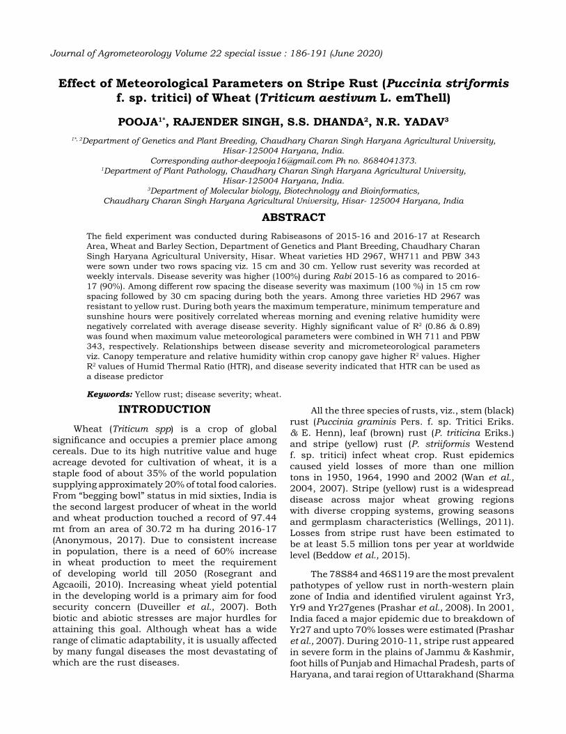
effect of Meteorological Parameters on Stripe rust (Puccinia striformis f. sp. tritici) of Wheat (Triticum aestivum L. emthell)

PooJa1*, raJeNder SINgh, S.S. dhaNda2, N.r. Yadav3

1*, 2Department of Genetics and Plant Breeding, Chaudhary Charan Singh Haryana Agricultural University, Hisar-125004 Haryana, India.

Corresponding [email protected] Ph no. 8684041373.1Department of Plant Pathology, Chaudhary Charan Singh Haryana Agricultural University,

Hisar-125004 Haryana, India.3Department of Molecular biology, Biotechnology and Bioinformatics,

Chaudhary Charan Singh Haryana Agricultural University, Hisar- 125004 Haryana, India

aBStraCtThe field experiment was conducted during Rabiseasons of 2015-16 and 2016-17 at Research Area, Wheat and Barley Section, Department of Genetics and Plant Breeding, Chaudhary Charan Singh Haryana Agricultural University, Hisar. Wheat varieties HD 2967, WH711 and PBW 343 were sown under two rows spacing viz. 15 cm and 30 cm. Yellow rust severity was recorded at weekly intervals. Disease severity was higher (100%) during Rabi 2015-16 as compared to 2016-17 (90%). Among different row spacing the disease severity was maximum (100 %) in 15 cm row spacing followed by 30 cm spacing during both the years. Among three varieties HD 2967 was resistant to yellow rust. During both years the maximum temperature, minimum temperature and sunshine hours were positively correlated whereas morning and evening relative humidity were negatively correlated with average disease severity. Highly significant value of R2 (0.86 & 0.89) was found when maximum value meteorological parameters were combined in WH 711 and PBW 343, respectively. Relationships between disease severity and micrometeorological parameters viz. Canopy temperature and relative humidity within crop canopy gave higher R2 values. Higher R2 values of Humid Thermal Ratio (HTR), and disease severity indicated that HTR can be used as a disease predictor

Keywords: Yellow rust; disease severity; wheat.

INtroduCtIoN

Wheat (Triticum spp) is a crop of global significance and occupies a premier place among cereals. Due to its high nutritive value and huge acreage devoted for cultivation of wheat, it is a staple food of about 35% of the world population supplying approximately 20% of total food calories. From “begging bowl” status in mid sixties, India is the second largest producer of wheat in the world and wheat production touched a record of 97.44 mt from an area of 30.72 m ha during 2016-17 (Anonymous, 2017). Due to consistent increase in population, there is a need of 60% increase in wheat production to meet the requirement of developing world till 2050 (Rosegrant and Agcaoili, 2010). Increasing wheat yield potential in the developing world is a primary aim for food security concern (Duveiller et al., 2007). Both biotic and abiotic stresses are major hurdles for attaining this goal. Although wheat has a wide range of climatic adaptability, it is usually affected by many fungal diseases the most devastating of which are the rust diseases.

All the three species of rusts, viz., stem (black) rust (Puccinia graminis Pers. f. sp. Tritici Eriks. & E. Henn), leaf (brown) rust (P. triticina Eriks.) and stripe (yellow) rust (P. striiformis Westend f. sp. tritici) infect wheat crop. Rust epidemics caused yield losses of more than one million tons in 1950, 1964, 1990 and 2002 (Wan et al., 2004, 2007). Stripe (yellow) rust is a widespread disease across major wheat growing regions with diverse cropping systems, growing seasons and germplasm characteristics (Wellings, 2011).Losses from stripe rust have been estimated to be at least 5.5 million tons per year at worldwide level (Beddow et al., 2015).

The 78S84 and 46S119 are the most prevalent pathotypes of yellow rust in north-western plain zone of India and identified virulent against Yr3, Yr9 and Yr27genes (Prashar et al., 2008). In 2001, India faced a major epidemic due to breakdown of Yr27 and upto 70% losses were estimated (Prashar et al., 2007). During 2010-11, stripe rust appeared in severe form in the plains of Jammu & Kashmir, foot hills of Punjab and Himachal Pradesh, parts of Haryana, and tarai region of Uttarakhand (Sharma


and Saharan, 2011). Stripe rust continues to pose a threat to wheat cultivation worldwide (Sareen et al., 2012). These zones are selectively prone to yellow rust as the pathogen been reported to be prevalent at higher altitudes, cool and temperate regions. Weather has a very important role to play in the occurrence, development and spread of diseases. Temperature, precipitation, relative humidity, sunshine hours, rainfall and wind have the greatest influence on different plant diseases. When susceptible host and virulent pathotypes coexist under optimum conditions, the chances of disease epidemic increases. Knowledge on interaction of weather and disease can provide information on disease appearance, severity, spread and perpetuation. Disease prediction is of fundamental importance for the successful and efficient use of chemicals to manage rusts. Several rust disease prediction models have been developed using weather variables alone (Subba Rao et al., 1990) or in combinations with other biological parameters (Audsley et al., 2005). Severity of stripe rust is affected by different meteorological parameters and microclimate of crop. Therefore, there is a need to develop weather-based models locally to predict stripe rust outbreaks in Haryana and adjoining areas, the major wheat producing region in India. Microclimate modification can be useful in management of stripe rust as disease is highly influenced by microclimate of the crop. So keeping this in view, the experiments were conducted to study the effect of different meteorological parameters and microclimate on stripe rust severity.

MaterIaLS aNd MethodSField Experiments

Wheat varieties HD 2967, WH711 and PBW 343 were sown under two rows spacing viz.15 cm and 30 cm during rabiseasons of 2015-16 and 2016-17. The crop was raised as per recommendations of Chaudhary Charan Singh Haryana Agricultural University, Hisar. Daily meteorological observations on temperature (oC), relative humidity (%), sunshine hours (hrs/day) and rainfall (mm) were recorded at the Agro meteorological Observatory (29°10’N latitude, 75°46’E longitude and altitude of 215.2 mabove mean sea level).

Microclimatic parameters viz. canopy temperature and relative humidity within crop canopy was recorded under different treatments. Canopy temperature was measured at 1400

hours at weekly interval with the help of Infrared Thermometer. The Infrared Thermometer was held at 45o to the horizontal above the canopy so as to look in a downward direction towards the crop surface. The relative humidity was measured at 1400 hours at weekly interval with the help of Belfort Psychron. Stripe rust severity was recorded visually as the percentage of leaf area infected according to the modified Cobb’s or Peterson’s scale (Peterson et al., 1948).The disease was recorded on 15 and 30cm spacing sown in paired row of 2m length and per cent leaf area of plants affected by the disease were recorded at weekly intervals. Disease severity was calculated by using the following formulae:

Disease severity (%) =

Area of plant tissue in-fected X 100

Total area of plant

Correlation coefficients and step wise multiple regression analysis was conducted between stripe rust disease severity and different meteorological parameters viz., temperature (oC), relative humidity (%), sunshine hours (hrs/day) and rainfall (mm) (Table 2). Humid Thermal ratio (HTR) was calculated by using following formulae:

Humid Thermal Ratio (HTR) =

Mean relative humidityMean temperature

reSuLtS aNd dISCuSSIoNDisease severity

Disease severity was calculated on the basis of per cent per cent leaf area infected observations. Disease severity was higher (100%) during rabi 2015-16 as compared to 2016-17 (91%). Difference in disease severity was due to prevailing different weather conditions during both the years. Temperature and relative humidity were the key factors for stripe rust development. Among different varieties, due to varietal difference, variety HD 2967 was highly resistant to stripe rust, whereas variety PBW 343 and WH711 were susceptible to stripe rust. During 2015-16 and 2016-17, the disease severity was maximum in 15 cm row spacing (100 and 95%) followed by 30 cm row spacing (95 and 83%) in PBW 343. In WH711 disease severity was maximum (100 and 90%) in 15 cm row spacing followed by 30 cm (90% and 81%).The main reason for low disease severity in wider spacing was change in microclimate. As in narrow spacing relative humidity within canopy was higher (86 %) during early period

Vol. 22, Special Issue POOJA et al. 187

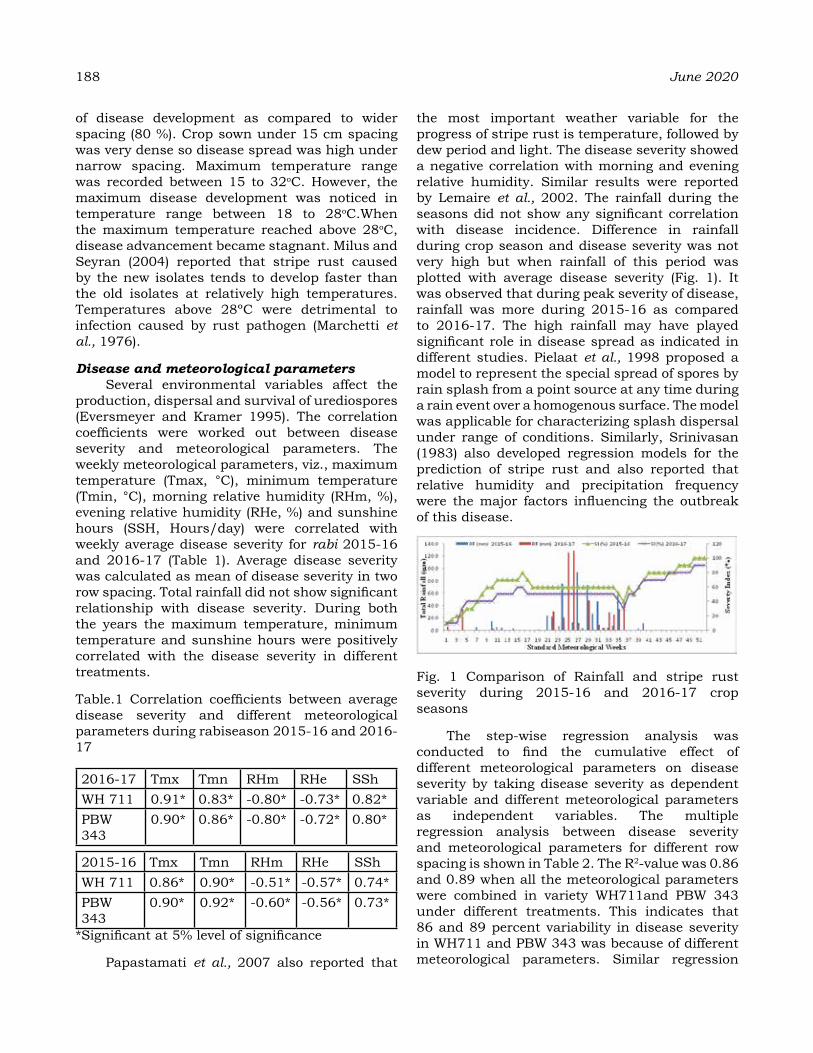
188 June 2020

of disease development as compared to wider spacing (80 %). Crop sown under 15 cm spacing was very dense so disease spread was high under narrow spacing. Maximum temperature range was recorded between 15 to 32oC. However, the maximum disease development was noticed in temperature range between 18 to 28oC.When the maximum temperature reached above 28oC, disease advancement became stagnant. Milus and Seyran (2004) reported that stripe rust caused by the new isolates tends to develop faster than the old isolates at relatively high temperatures. Temperatures above 28ºC were detrimental to infection caused by rust pathogen (Marchetti et al., 1976).

Disease and meteorological parameters Several environmental variables affect the

production, dispersal and survival of urediospores (Eversmeyer and Kramer 1995). The correlation coefficients were worked out between disease severity and meteorological parameters. The weekly meteorological parameters, viz., maximum temperature (Tmax, °C), minimum temperature (Tmin, °C), morning relative humidity (RHm, %), evening relative humidity (RHe, %) and sunshine hours (SSH, Hours/day) were correlated with weekly average disease severity for rabi 2015-16 and 2016-17 (Table 1). Average disease severity was calculated as mean of disease severity in two row spacing. Total rainfall did not show significant relationship with disease severity. During both the years the maximum temperature, minimum temperature and sunshine hours were positively correlated with the disease severity in different treatments.

Table.1 Correlation coefficients between average disease severity and different meteorological parameters during rabiseason 2015-16 and 2016-17

2016-17 Tmx Tmn RHm RHe SShWH 711 0.91* 0.83* -0.80* -0.73* 0.82* PBW 343

0.90* 0.86* -0.80* -0.72* 0.80*

2015-16 Tmx Tmn RHm RHe SShWH 711 0.86* 0.90* -0.51* -0.57* 0.74* PBW 343

0.90* 0.92* -0.60* -0.56* 0.73*

*Significant at 5% level of significance

Papastamati et al., 2007 also reported that

the most important weather variable for the progress of stripe rust is temperature, followed by dew period and light. The disease severity showed a negative correlation with morning and evening relative humidity. Similar results were reported by Lemaire et al., 2002. The rainfall during the seasons did not show any significant correlation with disease incidence. Difference in rainfall during crop season and disease severity was not very high but when rainfall of this period was plotted with average disease severity (Fig. 1). It was observed that during peak severity of disease, rainfall was more during 2015-16 as compared to 2016-17. The high rainfall may have played significant role in disease spread as indicated in different studies. Pielaat et al., 1998 proposed a model to represent the special spread of spores by rain splash from a point source at any time during a rain event over a homogenous surface. The model was applicable for characterizing splash dispersal under range of conditions. Similarly, Srinivasan (1983) also developed regression models for the prediction of stripe rust and also reported that relative humidity and precipitation frequency were the major factors influencing the outbreak of this disease.

Fig. 1 Comparison of Rainfall and stripe rust severity during 2015-16 and 2016-17 crop seasons

The step-wise regression analysis was conducted to find the cumulative effect of different meteorological parameters on disease severity by taking disease severity as dependent variable and different meteorological parameters as independent variables. The multiple regression analysis between disease severity and meteorological parameters for different row spacing is shown in Table 2. The R2-value was 0.86 and 0.89 when all the meteorological parameters were combined in variety WH711and PBW 343 under different treatments. This indicates that 86 and 89 percent variability in disease severity in WH711 and PBW 343 was because of different meteorological parameters. Similar regression

models for predicting the stripe rust in central plain regions were developed by Dutta et al., (2008). Rader et al., (2007) developed two models to predict the occurrence of leaf rustcaused by Puccinia recondita using air temperature, relative humidity and precipitation.

Table. 2 Stepwise multiple regression analysis between average stripe rust disease severity (Y) and meteorological parameters (Pooled data of 2015-16 and 2016-17)

regression equation R2

WH711Y= -60.3 + 1.24Tmx + 7.47Tmn 0.81Y= -87.8 - 3.01Tmx + 11.4Tmn + 0.52RHm + 0.01RHe - 0.47RF + 4.44SSh

0.86

PBW343Y= -55.7 + 1.41Tmx + 7.70Tmn 0.86Y= -102.4-2.93Tmx+12.1Tmn+0.87RHm-0.15RHe-0.60RF+4.58SSh

0.89

Disease severity and micrometeorological parameters

Microclimate plays an important role in disease development and multiplication. Canopy temperature was found low in narrow spacing (15 cm) during the early period of disease development but with the advancement in disease canopy temperature was highest in narrow spacing and lowest in wider spacing (30 cm). The main reason of this change might be due to development of stripe rust pustules on leaves of crop which lead to decrease rate of transpiration in narrow spacing crop and resulted in higher canopy temperature in narrow spacing as compared to wider spacing. Duveiller et al., 2005 concluded that canopy temperature is one of the factors associated with increased infection and disease development. The maintenance of healthy tissues by plants enables them to maintain a lower canopy temperature which, in turn, helps against the pathogen which requires relatively high temperatures for faster growth and development. Relative humidity was highest in 15 cm sowing followed by 30 cm sown crop but with advancement in disease relative humidity was decreased in narrow spacing as compared to wider spacing due to necrosis of leaves caused by stripe rust. Higher relative humidity was more favourable for disease development. These observations indicated that microclimate and disease are interrelated as disease was influenced by microclimate during early stage of disease development but once the disease was

developed it influenced microclimate of crop.

Relationships were developed between disease severity and microclimatic parameters viz. canopy temperature and relative humidity within crop canopy as shown in Tables 3 and 4. Higher R2 -values in different treatments indicated that canopy temperature and relative humidity within crop influenced disease severity during both the crop seasons. From this analysis it is clear that wider spacing can be helpful to decrease the rate of disease severity in highly susceptible areas.

Table.3 Relationship between stripe rust disease severity (Y) and Canopy temperature (pooled data WH711 and PBW 343)

2015-16 regression equation R2

15 cm Y = -0.026X3 + 1.765X2 - 30.69X + 159.3

0.87

30 cm Y=-0.022X3 + 1.554X2- 28.35X + 150.2

0.89

2016-1715 cm Y= -0.020X3 + 1.379X2 -23.67X +

118.20.90

30 cm Y= -0.013X3 +0.809X -10.29X + 17.38

0.89

X2=Tmx & Tmnat 15-16th SMW (standard meteorological week) X3= Tmx & Tmnat 50-51st SMW (standard meteorological week) X= Tmx & Tmnat 47-49th SMW (standard meteorological week)

Table.4 Relationship between stripe rust disease severity (Y) and relative humidity within crop Canopy (pooled data WH711 and PBW 343)

2015-16 regression equation R2

15 cm Y = 0.007X3 - 1.668X2 + 115.7X - 2482

0.71

30 cm Y= 0.031X3- 6.754X2 + 472.3X -10728

0.60

2016-1715 cm Y = 0.000X3- 0.082X2 + 5.299X +

1.9680.76

30 cm Y = 0.000X3- 0.100X2 + 6.422X -30.61

0.73

X2= RHm & RHe at 15-16th SMW (standard meteorological week).

X3= RHm & RHeat 50-51st SMW (standard meteorological week)

X= RHm & RHe at 47-49th SMW (standard meteorological week)


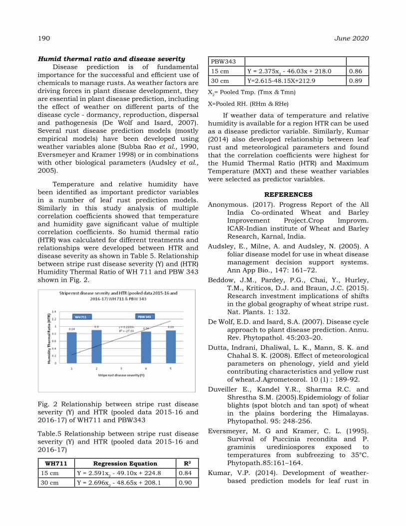
190 June 2020

Humid thermal ratio and disease severity Disease prediction is of fundamental

importance for the successful and efficient use of chemicals to manage rusts. As weather factors are driving forces in plant disease development, they are essential in plant disease prediction, including the effect of weather on different parts of the disease cycle - dormancy, reproduction, dispersal and pathogenesis (De Wolf and Isard, 2007). Several rust disease prediction models (mostly empirical models) have been developed using weather variables alone (Subba Rao et al., 1990, Eversmeyer and Kramer 1998) or in combinations with other biological parameters (Audsley et al., 2005).

Temperature and relative humidity have been identified as important predictor variables in a number of leaf rust prediction models. Similarly in this study analysis of multiple correlation coefficients showed that temperature and humidity gave significant value of multiple correlation coefficients. So humid thermal ratio (HTR) was calculated for different treatments and relationships were developed between HTR and disease severity as shown in Table 5. Relationship between stripe rust disease severity (Y) and (HTR) Humidity Thermal Ratio of WH 711 and PBW 343 shown in Fig. 2.

Fig. 2 Relationship between stripe rust disease severity (Y) and HTR (pooled data 2015-16 and 2016-17) of WH711 and PBW343

Table.5 Relationship between stripe rust disease severity (Y) and HTR (pooled data 2015-16 and 2016-17)

Wh711 regression equation R2

15 cm Y = 2.591x2 - 49.10x + 224.8 0.8430 cm Y = 2.696x2 - 48.65x + 208.1 0.90

PBW34315 cm Y = 2.375x2 - 46.03x + 218.0 0.8630 cm Y=2.615-48.15X+212.9 0.89

X2= Pooled Tmp. (Tmx & Tmn)

X=Pooled RH. (RHm & RHe)

If weather data of temperature and relative humidity is available for a region HTR can be used as a disease predictor variable. Similarly, Kumar (2014) also developed relationship between leaf rust and meteorological parameters and found that the correlation coefficients were highest for the Humid Thermal Ratio (HTR) and Maximum Temperature (MXT) and these weather variables were selected as predictor variables.

reFereNCeSAnonymous. (2017). Progress Report of the All

India Co-ordinated Wheat and Barley Improvement Project.Crop Improvm. ICAR-Indian institute of Wheat and Barley Research, Karnal, India.

Audsley, E., Milne, A. and Audsley, N. (2005). A foliar disease model for use in wheat disease management decision support systems. Ann App Bio., 147: 161–72.

Beddow, J.M., Pardey, P.G., Chai, Y., Hurley, T.M., Kriticos, D.J. and Braun, J.C. (2015). Research investment implications of shifts in the global geography of wheat stripe rust. Nat. Plants. 1: 132.

De Wolf, E.D. and Isard, S.A. (2007). Disease cycle approach to plant disease prediction. Annu. Rev. Phytopathol. 45:203–20.

Dutta, Indrani, Dhaliwal, L. K., Mann, S. K. and Chahal S. K. (2008). Effect of meteorological parameters on phenology, yield and yield contributing characteristics and yellow rust of wheat.J.Agrometeorol. 10 (1) : 189-92.

Duveiller E., Kandel Y.R., Sharma R.C. and Shrestha S.M. (2005).Epidemiology of foliar blights (spot blotch and tan spot) of wheat in the plains bordering the Himalayas. Phytopathol. 95: 248-256.

Eversmeyer, M. G and Kramer, C. L. (1995). Survival of Puccinia recondita and P. graminis urediniospores exposed to temperatures from subfreezing to 35°C. Phytopath.85:161–164.

Kumar, V.P. (2014). Development of weather-based prediction models for leaf rust in

wheat in the Indo-Gangetic plains of India. Eur J Plant Pathol. 140:429-40.

Lemaire, D., Huret, S., Calaym F and Maraite, H. (2002). Understanding P. striiformis west. Epidemics on winter wheat. Meded Rijksuniv Gent -FakLandlbourwkdToegep. Biol Wet. 67: 251-56.

Marchetti, M.A., Melching, J.S. and Bromfield, K.R. (1976). The effects of temperature and dew period on germination and infection by urediospores of Phakopsorapachyrhizi. Phytopathol.66:461-63.

Milus, E.A and Seyran, E. (2004). New races of Puccinia striiformis f. sp. tritici more aggressive than older races at 18 °C. In Proceedings of the 11th International Cereal Rusts and Powdery Mildews Conference. 22–27 August 2004, John Innes Centre, Norwich, UK. European and Mediterranean Cereal Rust Foundation, Wageningen, Netherlands. Cereal Rusts and Powdery Mildews Bulletin, Abstr. A2.50.

Papastamati, K., Bosch and Van den, F. (2007).The sensitivity of the epidemic growth rate to weather variables, with an application to yellow rust on wheat. Phytopath. 97: (2) : 202-210.

Peterson, R. E., Campbell, A. B and Hannah, A. E. (1948). A diagrammatic scale for estimating rust intensity of leaves and stems of cereals. Can J of Res. 26: 496–500.

Pielaat, A., Madden, L. V and Gort, G. (1998). Spores splashing under different environmental conditions: A Modeling Approach. Phytopath.88: 1131-39.

Prashar, M., Bhardwaj, S.C., Jain, S.K and Datta, D. (2007).Pathotypic evolution in Puccinia striiformis in India during 1995-2004. Aust. J. Agri. Res. 58:602-604.

Prashar, M., Bhardwaj, S.C., Jain, S.K., Sharma, Y.P and Mishra, B. (2008). Perspective on wheat rusts in India. In: 11th International Wheat Genetics Symposium. Appels, R.,

Eastwood, R., Lagudah, E., Langridge, P. and Lynne, M.M. (Eds.), held at Sydney, Australia, (http://hdl.handle.net/ 2123/3329).

Rader, T., Racca, P., Jorg, E and Hau, B. (2007). PUCREC/PUCTRIa decision support system for the control of leaf rust of winter wheat and winter rye. EPPO Bulletin, 37 (2) : 378–82.

Rosegrant, M. W and Agcaoili, M. (2010). Global Food Demand, Supply and Food Prospects.Washington, DC: International food policy research Institute.

Sareen, P., Sundeep, K., Uttam, K., Lakshman, P and Amit, K. S. (2012). Pathological and molecular characterizations of slow leaf rusting in fifteen wheat (Triticum aestivum L.) genotypes. Afri. J. of Biotechnol. 11:14956-14966.

Sharma, I and Saharan, M.S. (2011).Status of wheat diseases in India with a special reference to stripe rust. Plant Dis. Res. 26:0970-4914.

Srinivasan, G. (1983). Role of meteorological factors in the Epidemiology of Karnal bunt and rust diseases of wheat. M.Sc Thesis, Punjab Agricultural University, Ludhiana.

SubbaRao, K. V., Berggren, G. T and Snow, J. P. (1990).Characterization of wheat leaf rust epidemics in Louisiana. Phytopath. 80: 402–10.

Wan, A.M., Chen, X.M., He, Z.H. (2007).Wheat stripe rust in China. Aust. J. of Agri. Res.58:605–619.

Wan, A.M., Zhao, Z.H., Chen, X.M., He, Z.H. and Jin, S.L. (2004).Wheat stripe rust epidemic and virulence of Puccinia striiformisf. sp. Triticiin China in 2002. Pl. Dis. 88:896–904.

Wellings, C.R. (2011). Global status of stripe rust: a review of historical and current threats. Euphytica.179:129–141.


Calibration and validation of CereS-wheat model for North Western himalayas

raNu PathaNIa¹*, raJeNdra PraSad2, raNBIr SINgh raNa2, SudhIr KuMar MIShra3 aNd Saurav SharMa¹

¹Department of Agriculture, Himachal Pradesh2Department of Agronomy, Forages and Grassland Management, College of Agriculture, Chaudhary Sarvan Kumar

Krishi Vishvavidhalaya, Palampur (Himachal Pradesh) India3Punjab Agricultural University, Regional Research station, Faridkot (Punjab) India

*Corresponding author Email: [email protected]

aBStraCtA field experiment was conducted during rabi season 2015-16 and 2016-17 comprising four wheat varieties (viz., HS-490, VL-829, VL-892 and VL-907) grown on five different sowing dates (viz., 20th October, 5th November, 20th November, 5th December and 20th December) in split plot design with three replications at Department of Agronomy, Forages and Grassland Management farm, CSK HPKV, Palampur, Himachal Pradesh (India). The DSSAT-CERES-wheat (version 4.6) model was calibrated using various growth and yield parametrs collected from experiment conducted during 2015-16 while for validation, data collected from subsequent experiment (2016-17) have been used. The results of the present investigation revealed that among different treatments during 2015-16, the range of the observed and simulated yield was 3.3-5 t ha-¹ and 3.0-5.4 t ha-¹, respectively whereas during 2016-17, it was 2.6-3.8 t ha-¹ (observed) and 2.9-3.9 t ha-¹ (simulated). The mean observed and simulated grain yield was 3.1 to 3.9 t ha-¹ and 3.2 to 3.9 t ha-¹. For observed and simulated grain yield, standard deviation (SD) of 496 and 601 kg and coefficient of variation (CV) of 13 and 15 % has been recorded during 2015-16 while during 2016-17, it was 441 and 247 kg (SD) and 13 and 8 % (CV). Likewise, observed and simulated above ground biomass was 8.3-12.4 t ha-¹ and 8.2-12.9 t ha-¹ during 2015-16 and 6.5-12.0 t ha-¹ and 6.0-11.9 t ha-¹ 2016-17, respectively. Among the treatments, mean simulated biological yield was 10.2 and 7.9 t ha-¹ while, observed was 9.9 and 8.3 t ha-¹. For observed and simulated biomass production, 1303 and 1507 kg SD and 13 and 15 % CV was recorded during 2015-16 but during 2016-17, it was 1670 and 1873 (SD) and 20 and 24 % (CV), respectively. During both the years, between observed and simulating grain yield, high correlation coefficient (r= 0.76 & 0.85), low RMSE (381 & 281 kg), nRMSE (9.6 & 8.9 %), MBE (-0.5 & 77.3 kg) and MAPE (0.06 & 3.5 %) confirmed the accurate simulation by model. High simulated and observed grain yield was obtained if variety HS-490 (2015-16) and VL-907 (2016-17) were sown on 20th November. Similarly, for observed and simulated biomass production high correlation coefficient, (r =0.89 and 0.98) and low RMSE (735 and 591 kg), nRMSE (7.4 and 7.0 %), MBE (316 and 453 kg) and MAPE (3.2 and -5.9 %), have been recorded, among the treatments. Thus, the grain yield and above ground biomass of wheat cultivars were fairly simulated by the DSSAT model hence, it may be used for crop yield simulations under varying input conditions of mid hill region of Himachal Pradesh.

Keywords: DSSAT-CSM-CERES model, cultivars, simulation, sowing date, wheat, etc.

INtroduCtIoN

Wheat (Triticum aestivum L.) is an important cereal crop after rice in India grown on about 29.58 million hectares area with 3.37 tonnes ha-¹ an average productivity (FAO, 2018). Being the world’s second important cereal crop after rice, wheat crop provides around 20% of global protein requirement in human diet and extremely important staple foods to over 10 billion people all over the world. In Himachal Pradesh it covers an area of 0.321 million hectares with 0.605 million tonnes production during 2016-17 (Anonymous, 2018-19). Wheat is a long day thermo sensitive

crop which requires cool climate during early growth stages and very less heat stress at later development phases (Farooq et al., 2011). There is likely influence in spatial and temporal trends of temperature and rainfall due to global climate changes, which will affect crop phenology (Jalota and Vashisht, 2016) and wheat yield (Mishra et al., 2015). In Himachal Pradesh, timely sowing of wheat crop on 20th November recorded 5.2 % increased grain yield than early sown (5th November) crop however, late (20th December) sowing caused to declined grain yield by 27.5 % (Pathania et al., 2018).


In agricultural research crop simulation models play key role in developing the decision making research, technology management and policy options. It acts as useful tool to predict the growth, development and productivity of a crop under varying soil, crop input and climatic conditions. In modelling system, decision support system for agrotechnology transfer (DSSAT v4.6) is well accepted cropping system model (CSM) included around 40 crops. Already, in worldwide DSSAT model has been successfully evaluated in fertilizer management under diverse management and climates strategies (Zalud et al., 2001), irrigation scheduling (Dar et al., 2017) and environmental impact assessment (Hoffmann and Ritchie, 1993). Looking into the usefulness of models in developing suitable management practices, the present investigation of calibration and validation of DSSAT v. 4.6 model for popular wheat cultivars has been carried out under varying environments of Himachal Pradesh (India).

MaterIaLS aNd MethodSA field investigation has been conducted at

Department of Agronomy, Forages and Grassland Management farm, CSK HPKV, Palampur, Himachal Pradesh (latitude 32o 6’ N, longitude 76o 3’ E and altitude about 1290.8 m above sea level) during the rabi seasons of 2015-16 and 2016-17. The experiment was conducted in split plot design with five dates of sowing (20th October, 5th November, 20th November, 5th December and 20th December) in main plots and four varieties of wheat (viz. VL-829, VL-907, VL-892 and HS-490) in sub-plots with three replications. Daily meteorological data viz., rainfall (mm), maximum

and minimum relative humidity (%), maximum and minimum temperature (°C), duration of bright sunshine (hours), wind speed (kmh-¹) etc. were recorded from Agrometeorological observatory, CSK HPKV, Palampur.

Agro-climatically, the experimental area falls under sub-temperate and sub-humid zone, which is distinguished by acute winters (3.5-13.4oC) and high rainfall with mild summers (19.0-31oC). The average rainfall of the area is 2500 mm and its 78 per cent amount is received during monsoon (June to September) period. In general, the period of south west monsoon onset is the last week of June. Winter rains usually occurs during December to February by western disturbance. During first year (2015-16) crop season (October to May), minimum temperature ranged from 1.7 to 19.4°C and maximum temperature was 14.3 to 32.7°C however during 2016-17, it was 14.6 to 32.1°C and 1.7 to 18.9°C, respectively. Well distributed rainfall of 435.6 and 481 mm was experienced by crop during 2015-16 and 2016-17. Range of the sunshine duration was 3.4-11.0 hours day-¹ (2015-16) and 2.3-10.6 hours day-¹ (2016-17).

Cultivar specific genetic coefficient of every wheat cultivar (VL-829, VL-907, VL-892 and HS-490) were derived following the repeated iterations until a close match between observed and simulated phenology, growth and yield were achieved in the model calculations. The model was calibrated for phenology (days taken to anthesis and maturity), grain yield and biological yield using experimental data recorded during 2015-16 that were validated from the data generated

Table 1: Statistical measures for model evaluationS.No. Statistical parameter Formula Reference 1 Correlation coefficient (r) (Kirch, 2008)

2 Root mean square error (RMSE) (Thomann, 1982)

3 Normalized root mean square error (nRMSE) (Loague and Green, 1991)

4 Mean bias error (MBE) (Panda et al., 2003)

5 Mean absolute percentage error (MAPE) (Panda et al., 2003)

where, Oi and Pi are observed and predicted values, respectively. Ō is the observed mean, P is the predicted mean.

Vol. 22, Special Issue PATHANIA et al. 193

194 June 2020

during 2016-17. For the evaluation of the model performance different statistical measures like correlation coefficient (r), root mean square error (RMSE), normalized RMSE, mean bias error (MBE) and mean absolute percentage error (MAPE) were used (Table 1).

reSuLtS aNd dISCuSSIoNCalibration of DSSAT model

Model calibration is the refinement of the model variables to obtain error-free simulated output close to the observed data. Because, simulated values and the observed data do not exactly comply with each other so, minor adjustments for some parameters have to be made. For calibration of the DSSAT-CERES wheat model, field experimental data generated during 2015-16 have been used. The genetic coefficients required in the CERES wheat model for four different cultivars of wheat were obtained by using available input parameters for each genotypes and running the model iteratively till the predicted grain and biological yields showed variation less than 10% of the observed values. The derived genetic coefficients of wheat crop for all cultivars used for simulation of different date of sowing have been presented in Table 2.

validation of dSSat modelGrain yield

Both years in different treatments, deviation of -0.6 to + 0.8 t ha-¹ and -0.4 to +0.6 t ha-¹ have been appeared between observed and simulated grain yield. During 2015-16, simulated yield ranged from 3.0 to 5.4 t ha-¹ and range of observed yield was between 3.3 and 5.0 t ha-¹, among different treatment combinations (Fig. 1 a). While, during 2016-17 the range of simulated yield was between 2.9 and 3.9 t ha-¹ that was between 2.6 and 3.8 t ha-¹ for observed yield (Fig. 1 b). The simulated mean grain yield was 3.9 and 3.2 t ha-¹ and observed was 3.9 and 3.1 t ha-¹ with a standard deviation (SD) of 601 and 496 kg and coefficient of variation (CV) of 15 and 13 % for the simulated and observed grain yield during 2015-16. During, 2016-17, the SD was 247 and 441 kg however; CV was 8 and 13.0 %, respectively, for the simulated and observed grain yield (Table 3). Ottman et al. (2012) also reported 6.9% declined grain yield with 1°C increase above 16.3°C in seasonal temperature and thus, they concluded that possible future increase in temperature could perhaps cause to yield reduction of wheat and the late sown wheat are expected to be affected more drastically. The model performance was found to

Table 2: Genetic coefficients of the wheat cultivars

Code description HS-490 vL-829 vL-892 vL-907PIV Days at optimum vernalizing temperature required to com-

plete vernalization. 19 22 20 18

PID Percentage reduction in development rate in a photoperiod 10 hour shorter than the threshold relative to that at the threshold.

45 60 55 60

P5 Grain filling (excluding lag) phase duration (°C.d) 800 850 600 748G1 Kernel number per unit canopy weight at anthesis (No. /g) 21 20 20 19G2 Standard kernel weight under optimum conditions (mg) 38 25 37 28G3 Standard, non-stressed dry weight (total, including grain) of

a single tiller at maturity (g) 6.5 7.8 6.0 7.5

PHINT Interval between successive leaf tip appearances (oC. d) 25 34 28 30

Table 3: Performance of DSSAT-CERES-Wheat model for simulating yield of wheat

Parameters Simulated observed Simulated vs observedMean Sd Cv Mean Sd Cv r rMSe nrMSe MBe MaPe

2015-16Grain yield (kg ha-¹) 3981 601 15 3982 496 13 0.76 381 9.6 -0.5 0.06Biological yield (kg ha-¹) 10253 1507 15 9936 1303 13 0.89 735 7.4 316 3.22016-17Grain yield (kg ha-¹) 3231 247 8 3154 441 13 0.85 281 8.9 77.3 3.5Biological yield (kg ha-¹) 7938 1873 24 8391 1670 20 0.98 591 7.0 -453 -5.9

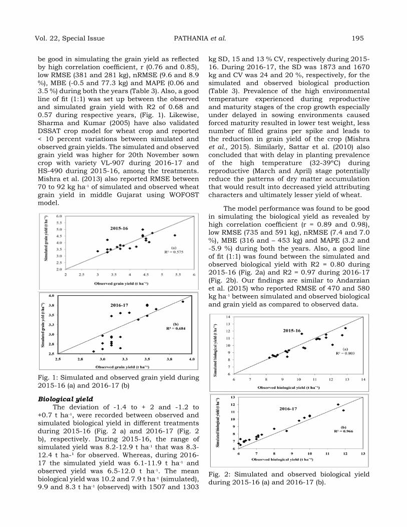
be good in simulating the grain yield as reflected by high correlation coefficient, r (0.76 and 0.85), low RMSE (381 and 281 kg), nRMSE (9.6 and 8.9 %), MBE (-0.5 and 77.3 kg) and MAPE (0.06 and 3.5 %) during both the years (Table 3). Also, a good line of fit (1:1) was set up between the observed and simulated grain yield with R2 of 0.68 and 0.57 during respective years, (Fig. 1). Likewise, Sharma and Kumar (2005) have also validated DSSAT crop model for wheat crop and reported < 10 percent variations between simulated and observed grain yields. The simulated and observed grain yield was higher for 20th November sown crop with variety VL-907 during 2016-17 and HS-490 during 2015-16, among the treatments. Mishra et al. (2013) also reported RMSE between 70 to 92 kg ha-¹ of simulated and observed wheat grain yield in middle Gujarat using WOFOST model.

Fig. 1: Simulated and observed grain yield during 2015-16 (a) and 2016-17 (b)

Biological yieldThe deviation of -1.4 to + 2 and -1.2 to

+0.7 t ha-¹, were recorded between observed and simulated biological yield in different treatments during 2015-16 (Fig. 2 a) and 2016-17 (Fig. 2 b), respectively. During 2015-16, the range of simulated yield was 8.2-12.9 t ha-¹ that was 8.3-12.4 t ha-¹ for observed. Whereas, during 2016-17 the simulated yield was 6.1-11.9 t ha-¹ and observed yield was 6.5-12.0 t ha-¹. The mean biological yield was 10.2 and 7.9 t ha-¹ (simulated), 9.9 and 8.3 t ha-¹ (observed) with 1507 and 1303

kg SD, 15 and 13 % CV, respectively during 2015-16. During 2016-17, the SD was 1873 and 1670 kg and CV was 24 and 20 %, respectively, for the simulated and observed biological production (Table 3). Prevalence of the high environmental temperature experienced during reproductive and maturity stages of the crop growth especially under delayed in sowing environments caused forced maturity resulted in lower test weight, less number of filled grains per spike and leads to the reduction in grain yield of the crop (Mishra et al., 2015). Similarly, Sattar et al. (2010) also concluded that with delay in planting prevalence of the high temperature (32-39ºC) during reproductive (March and April) stage potentially reduce the patterns of dry matter accumulation that would result into decreased yield attributing characters and ultimately lesser yield of wheat.

The model performance was found to be good in simulating the biological yield as revealed by high correlation coefficient (r = 0.89 and 0.98), low RMSE (735 and 591 kg), nRMSE (7.4 and 7.0 %), MBE (316 and – 453 kg) and MAPE (3.2 and -5.9 %) during both the years. Also, a good line of fit (1:1) was found between the simulated and observed biological yield with R2 = 0.80 during 2015-16 (Fig. 2a) and R2 = 0.97 during 2016-17 (Fig. 2b). Our findings are similar to Andarzian et al. (2015) who reported RMSE of 470 and 580 kg ha-¹ between simulated and observed biological and grain yield as compared to observed data.

Fig. 2: Simulated and observed biological yield during 2015-16 (a) and 2016-17 (b).

Vol. 22, Special Issue PATHANIA et al. 195

196 June 2020

CoNCLuSIoNWheat is one of the most important staple

cereal crops. Besides the biotic and abiotic stress factors determination of the location specific optimum sowing time of high yielding cultivars are pre requisite. The models are effective tools for crop growth and yield assessment under varying input conditions. Among the treatments, observed grain yield was 2.6 - 5.0 t ha-¹ and simulated yield was 2.9-5.4 t ha-¹. High observed (8.3-12.4 t ha-¹) and simulated above ground biomass (8.2-12.9 t ha-¹) have been recorded during previous year crop. For higher grain and biological yield of wheat, cultivars VL-907 and/or HS-490 may be sown around 20th November. Among the years, maximum root mean square errors of 381 for grain yield and 735 for biological yield confirmed the accurate simulation by the DSSAT-CERES wheat model. Therefore DSSAT model may be judicially used for growth and yield simulations under varying sowing environments of mid-hill conditions of Himachal Pradesh.

reFereNCeSAndarzian, B., Hoogenboom, G., Bannayan,

M., Shirali, M. and Andarzian, B. (2015). Determining optimum sowing date of wheat using CSM-CERES-wheat model. J. Saudi Soc. of Agril Sci. 14: 189-99.

Anonymous (2018-19). Economic survey of Himachal Pradesh (2018-2019) : pp 41-45.

Dar, E.A., Brar, A.S., Mishra, S.K. and Singh K.B. (2017). Simulating response of wheat to timing and depth of irrigation water in drip irrigation system using CERES-Wheat model. Field Crops Res. 214:149–163

FAO (2018). Food and Agriculture Organization of the United Nations. http://FAOSTAT.fao.org

Farooq, M., Breley, H. and Palta, J.A. (2011). Heat stress in wheat during reproductive and grain–filling phases. Plant Sci., 30:1–17.

Hoffmann, F. and Ritchie, J.T. (1993). Model for Slurry and Manure in CERES and Similar Models. J. Agron. and Crop Sci., 170, 330-340.

Jalota, S.K. and Vashisht, B.B. (2016). Adapting cropping systems to future climate change scenario in three agro-climatic zones of Punjab, India. J. Agrometeorol. 18 (1) : 48-56.

Kirch, W. (2008). Pearson’s Correlation Coefficient. Encyclopedia of Public Health, pp. 1090-1091.

Loague, K. and Green, R.E. (1991). Statistical and graphical methods for evaluating solute transport models; Overview and Application. J. Contaminant Hydrol. 7: 51–73.

Mishra, S.K., Shekh, A.M., Pandey, V., Yadav, S.B. and Patel, H.R. (2015). Sensitivity analysis of four wheat cultivars to varying photoperiod and temperature at different phenological stages using WOFOST model. J. Agrometeorol. 17 (1) : 74-79.

Mishra S.K., Shekh A.M., Yadav S.B., Kumar A., Pandey V. and Patel H.R. (2013). Simulation of growth and yield of four wheat cultivars using WOFOST model under middle Gujarat region. J. Agrometeorol. 15:1 43-50.

Ottman, M.J., Kimball, B.A., White, J.W. and Wall, G.W. (2012). Wheat Growth Response to Increased Temperature from Varied Planting Dates and Supplemental Infrared Heating. Agron. J. 104 (1) : 07-16.

Panda, R.K., Behera S.K. and Kashyap P.S. (2003). Effective management of irrigation water for wheat under stressed conditions. Agril. Water Manag. 63: 37-56.

Pathania, R., Prasad R., Rana R.S., Mishra S. and Sharma S. (2018). Growth and yield of wheat as influenced by dates of sowing and varieties in north western Himalayas. J Pharmacogn Phytochem. 7 (6) : 517-520

Sattar, A., Cheema, M.A., Farooq, M., Wahid, M.A., Wahid, A. and Babar, B.H. (2010). Evaluating the performance of wheat varieties under late sown conditions. Int. J. Agric. Biol., (12) : 561–565.

Sharma, H.L. and Kumar, R. (2005). Effect of sowing dates on dry matter accumulation, growth and yield of wheat (Triticum aestivum) varieties in North- western Himalayas. J. Agron. 31:2 2-8.

Thomann, R.V. (1982). Verification of water quality models. J. Environ. Eng.108: 923-40.

Zalud, Z, Stralkova, R., Pokorny, E. and Podesvova, J. (2001). Estimation of Winter Wheat Nitrogen Stress Using the CERES Crop Model. Rostlinna Vyroba, 47: 253- 259.

estimation of reference evapotranspiration (eto) and Crop Water requirement of Soybean and Cotton For Marathwada region

S. v. Phad1, K. K. daKhore2, r. S. SaYYad3, NIteSh aWaShthI4 aNd r. BaLaSuBraMaNIaM5

1, 3Department of Agricultural Meteorology, 2AICRP on Agricultural Meteorology, VNMKV, Parbhani (M.S).

Vasantrao Naik Marathwada Krishi Vidyapeeth, Parbhani-431 402 (M.S.), India.4Senior Research Fellow, IMD, New Delhi

5Agrimet Division, IMD, PuneEmail: [email protected]

aBStraCtThe reference evapotranspiration (ETo) is an important agrometeorological parameter which has been used in a number of applications in agriculture. In present study daily, weekly, monthly, seasonal, and annual ETo was determined for seven districts of Marathwada region having long period (29-35 years) weather data by Hargreaves method. The Kc values for soya bean and cotton as given in FAO-56 was used to calculate the daily crop water requirement (ETc). The results revealed that, ETo increases continuously from January and reaches to its maximum during May, but there is quite differences among the districts. The ETo reaches to its peak value during 28th April to 18th May at all the districts of Marathwada region. During June ETo decreases sharply and remains low during July and August and with slight increase during month of September, it decreases afterwards. In summer season when the temperature and wind speed both are highest so the total ETo was maximum, while in kharif season there may be wind speed is high but temperature comparatively lower than the summer due to rainfall thereby less ETo. Among the districts on daily, weekly, monthly, seasonal and annual basis Parbhani had highest ETo and Aurangabad had lowest ETo followed by Nanded, Latur, Osmanabad, Beed and Jalna. The mean water requirement (ETc) of soybean during initial stage was found to be lower (2.09 to 2.29 mm day-1) and it increased during developmental stage (3.37 to 3.75 mm day-1) and during mid season stage (4.90 to 5.32 mm day-1) and decreased during late-season stage (2.25 to 2.41 mm day-1). The total water requirement across the districts varies between Parbhani (457.81 mm) to Aurangabad (419.60 mm). The mean water requirement of cotton during initial stage (1.77 to 1.95 mm day-1), during developmental stage (3.42 to 3.78 mm day-1), during mid season stage (5.09 to 5.46 mm day-1) and during late season stage it decreases (1.94 to 2.09 mm day-1). The total water requirement of cotton varies between Parbhani (687.88 mm) and Aurangabad (638.80 mm)

Keywords: Reference evapotranspiration, Hargreaves method, Water requirement, Soybean, Cotton

INtroduCtIoN

Water is one of the most essential natural resource which plays a vital role in maintaining biodiversity, our health, social welfare and our economic development (Donald, 1968). Evapotranspiration is the combination of two separate processes commonly known as evaporation and transpiration. In this process water is lost on the one hand from the top soil or water surface by evaporation (physical process) and on the other hand from the crop plant tissues through transpiration (biological process). Both evaporation and transpiration occurs simultaneously therefore, no easy way of distinguishing between these two processes.

Reference evapotranspiration (ETo) is a major component in agricultural water management, irrigation scheduling as well as water resource planning. The reference evapotranspiration (ETo) flux occurring from cropped land surfaces are essential in studies relating to hydrology, climate and agricultural water management. The successful irrigation scheduling mainly depends upon the correct estimation of evapotranspiration. The prediction of evapotranspiration is based on meteorological variables like temperature, humidity, sunshine hour, wind speed. By applying a crop coefficient (Kc) values, this ETo can be used to estimate the crop evapotranspiration (ETc).

Estimation of crop water requirement is one of the main component used in irrigation


198 June 2020

planning, design and operation (Rowshon et al., 2013). Crop water requirement vary mainly due to variation in growth stages and climatic conditions. Understanding and determining crop evapotranspiration (ETc) is essential for scheduling irrigation to meet the crop water use demand and to optimize crop production. Jensen et al., (1990) provided detailed reviews of the methods commonly used to determine evapotranspiration and estimated crop water requirements.

The Marathwada region forms a Deccan Plateau, climate is very dry and subject to extremes, depends on judicious use of water resources as fresh water for human consumption and agriculture due to uneven distribution of rainfall. To meet the future food demands and growing competition for clean water, a more effective use of water in both irrigated and rainfed agriculture will be essential.

MaterIaL aNd MethodSLocation of Study Area

The Marathwada region of Maharashtra states comprises of eight districts total area of 64818 sq km geographically lies between 17o35’ to 20o 40’ latitude and 74o 40’ to 78o10’ longitude. The altitude ranges between 300 to 900 meter above mean sea level (MSL). The present study is conformed to Marathwada region comprising of 8 districts with an total geographical area is 64.5 lakh ha with 57.0 lakh ha land suitable for agriculture.

Table 3.1: Detailed information of different districts of Marathwada Region

Districts Latitude Longitude Altitude (m)

Data Availabil-ity

PARBHANI 19o16’ 76o46’ 423.50 1982-2017

AURANGAB-AD

19o51’ 75o24’ 586.60 1982-2010

JALNA 19o50’ 75o48’ 534.00 1982-2010

NANDED 19o05’ 77o20’ 358.40 1982-2010

OSMANABAD 18o10’ 76o03’ 662.89 1982-2010

LATUR 18o04’ 77o07’ 639.80 1982-2010

BEED 19o00’ 75o43’ 519.00 1982-2010

Collection of Meteorological Data Daily weather data of maximum and

minimum temperature of selected districts for at least 29 to 35 years period was collected from India Meteorological Department (IMD), Pune. Due to unavailability of Hingoli district data, this district is not taken into study.

Processing of Data The collected data of each district were used

to work out mean of each parameter of each district and then those daily mean data used to calculate reference evapotranspiration (ETo) on daily, weekly, monthly, seasonal and annual basis. The daily crop water requirement (ETc) was determined by multiplying daily ETo of each districts with Kc, determined for each crop. Thus daily ETc computed were summed for different growth stages of crop and total seasonal crop water was determined.

Selection of CropsIn order to workout crop water requirement

Soybean and Cotton crops were selected.

Estimation of Reference Evapotranspiration (ETo)

Temperature Based Method

Hargreaves method: Hargreaves developed a method in 1985 to estimate evapotranspiration is an empirical relation based on air temperature and radiation. (Bsanagouda R. F., 2016). The Hargreaves method is given by:

ETo = 0.0023 RA Td0.5 (Tm + 17.8)

Where, ETo is reference evapotranspiration (mm day-1)

RA is extra-terrestrial radiation (mm day-1)

Td is difference between max. and min temp. (oC)

Tm is mean temperature (oC)

Crop Evapotranspiration/ Crop Water Requirement (ETc)

Water requirement of encompass the total amount of water used in evapotranspiration. Out of the total evapotranspiration, evaporation account for about 10 percent and plant transpiration for the remaining 90 percent.

ETc = Kc ETo

Where,

ETc = crop evapotranspiration/Crop water requirement, (mm day-1),

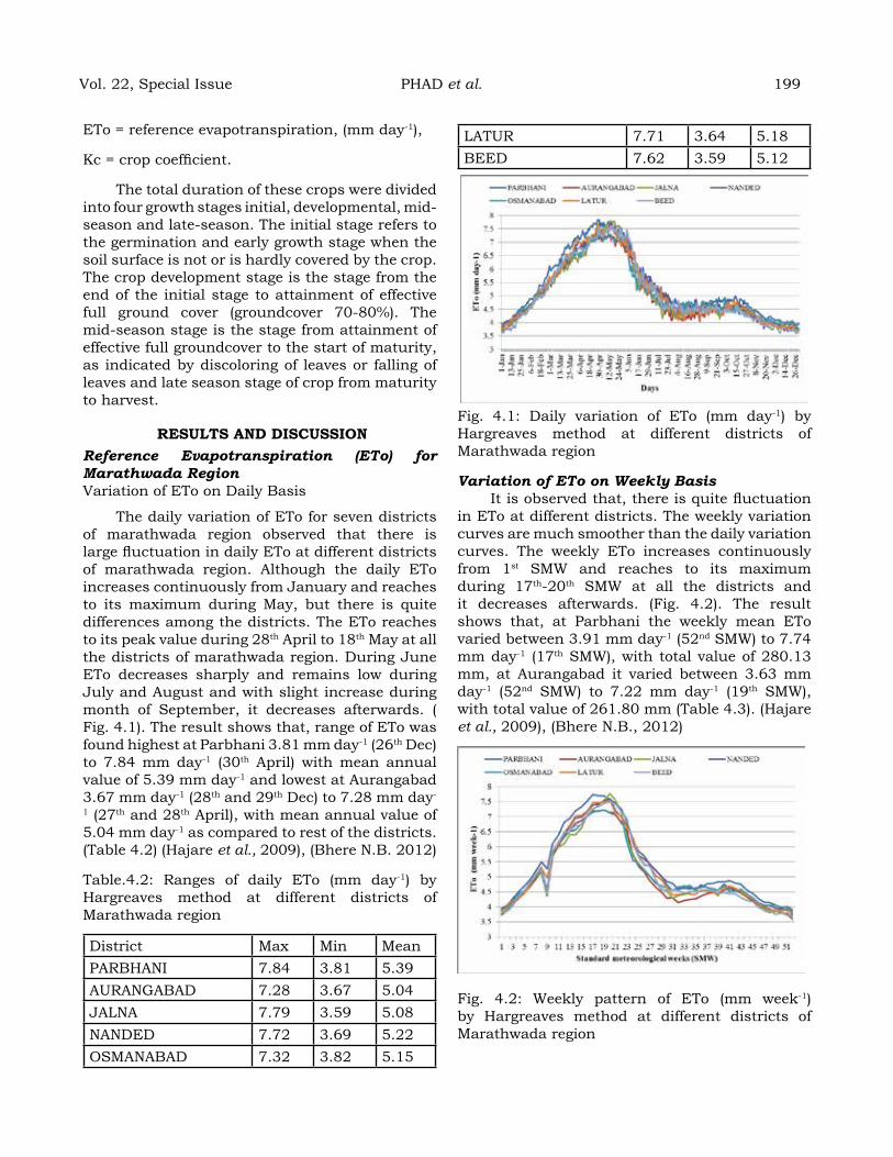
ETo = reference evapotranspiration, (mm day-1),

Kc = crop coefficient.

The total duration of these crops were divided into four growth stages initial, developmental, mid-season and late-season. The initial stage refers to the germination and early growth stage when the soil surface is not or is hardly covered by the crop. The crop development stage is the stage from the end of the initial stage to attainment of effective full ground cover (groundcover 70-80%). The mid-season stage is the stage from attainment of effective full groundcover to the start of maturity, as indicated by discoloring of leaves or falling of leaves and late season stage of crop from maturity to harvest.

reSuLtS aNd dISCuSSIoNReference Evapotranspiration (ETo) for Marathwada RegionVariation of ETo on Daily Basis

The daily variation of ETo for seven districts of marathwada region observed that there is large fluctuation in daily ETo at different districts of marathwada region. Although the daily ETo increases continuously from January and reaches to its maximum during May, but there is quite differences among the districts. The ETo reaches to its peak value during 28th April to 18th May at all the districts of marathwada region. During June ETo decreases sharply and remains low during July and August and with slight increase during month of September, it decreases afterwards. ( Fig. 4.1). The result shows that, range of ETo was found highest at Parbhani 3.81 mm day-1 (26th Dec) to 7.84 mm day-1 (30th April) with mean annual value of 5.39 mm day-1 and lowest at Aurangabad 3.67 mm day-1 (28th and 29th Dec) to 7.28 mm day-

1 (27th and 28th April), with mean annual value of 5.04 mm day-1 as compared to rest of the districts. (Table 4.2) (Hajare et al., 2009), (Bhere N.B. 2012)

Table.4.2: Ranges of daily ETo (mm day-1) by Hargreaves method at different districts of Marathwada region

District Max Min MeanPARBHANI 7.84 3.81 5.39AURANGABAD 7.28 3.67 5.04JALNA 7.79 3.59 5.08NANDED 7.72 3.69 5.22OSMANABAD 7.32 3.82 5.15

LATUR 7.71 3.64 5.18BEED 7.62 3.59 5.12

Fig. 4.1: Daily variation of ETo (mm day-1) by Hargreaves method at different districts of Marathwada region

Variation of ETo on Weekly BasisIt is observed that, there is quite fluctuation

in ETo at different districts. The weekly variation curves are much smoother than the daily variation curves. The weekly ETo increases continuously from 1st SMW and reaches to its maximum during 17th-20th SMW at all the districts and it decreases afterwards. (Fig. 4.2). The result shows that, at Parbhani the weekly mean ETo varied between 3.91 mm day-1 (52nd SMW) to 7.74 mm day-1 (17th SMW), with total value of 280.13 mm, at Aurangabad it varied between 3.63 mm day-1 (52nd SMW) to 7.22 mm day-1 (19th SMW), with total value of 261.80 mm (Table 4.3). (Hajare et al., 2009), (Bhere N.B., 2012)

Fig. 4.2: Weekly pattern of ETo (mm week-1) by Hargreaves method at different districts of Marathwada region

Vol. 22, Special Issue PHAD et al. 199

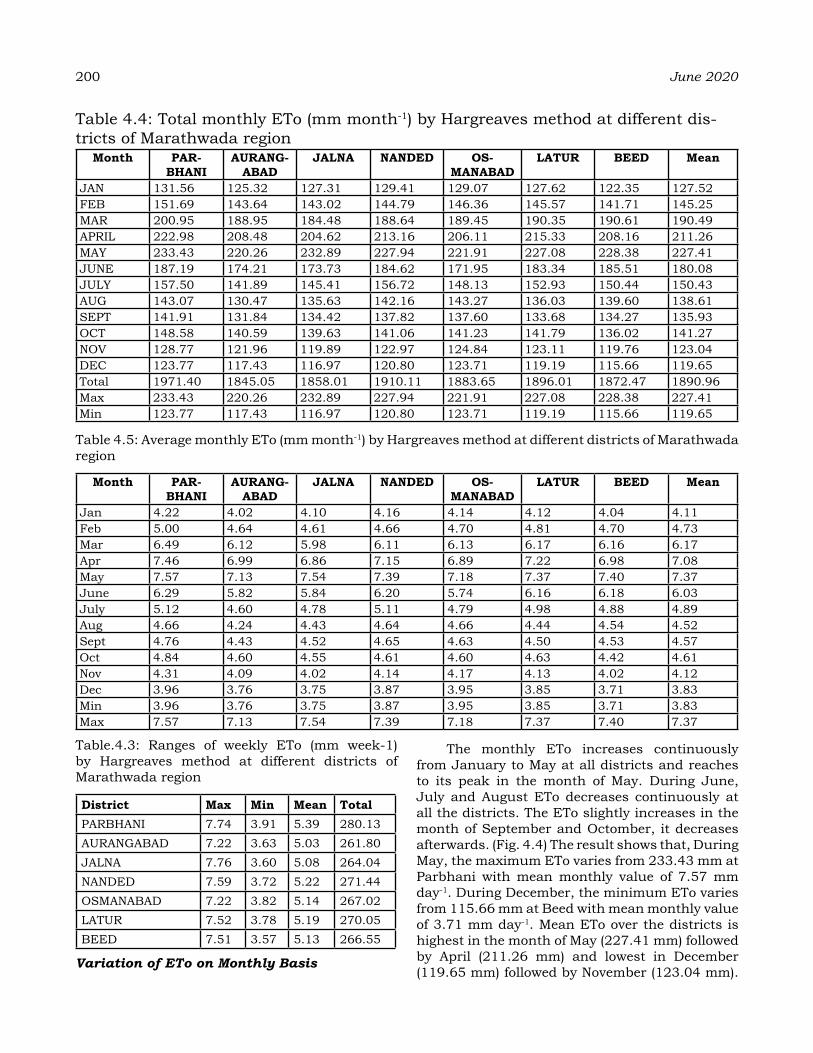
200 June 2020

Table.4.3: Ranges of weekly ETo (mm week-1) by Hargreaves method at different districts of Marathwada region

district Max Min Mean totalPARBHANI 7.74 3.91 5.39 280.13AURANGABAD 7.22 3.63 5.03 261.80JALNA 7.76 3.60 5.08 264.04NANDED 7.59 3.72 5.22 271.44OSMANABAD 7.22 3.82 5.14 267.02LATUR 7.52 3.78 5.19 270.05BEED 7.51 3.57 5.13 266.55

Variation of ETo on Monthly Basis

The monthly ETo increases continuously from January to May at all districts and reaches to its peak in the month of May. During June, July and August ETo decreases continuously at all the districts. The ETo slightly increases in the month of September and Octomber, it decreases afterwards. (Fig. 4.4) The result shows that, During May, the maximum ETo varies from 233.43 mm at Parbhani with mean monthly value of 7.57 mm day-1. During December, the minimum ETo varies from 115.66 mm at Beed with mean monthly value of 3.71 mm day-1. Mean ETo over the districts is highest in the month of May (227.41 mm) followed by April (211.26 mm) and lowest in December (119.65 mm) followed by November (123.04 mm).

Table 4.4: Total monthly ETo (mm month-1) by Hargreaves method at different dis-tricts of Marathwada region

Month Par-BhaNI

auraNg-aBad

JaLNa NaNded oS-MaNaBad

Latur Beed Mean

JAN 131.56 125.32 127.31 129.41 129.07 127.62 122.35 127.52FEB 151.69 143.64 143.02 144.79 146.36 145.57 141.71 145.25MAR 200.95 188.95 184.48 188.64 189.45 190.35 190.61 190.49APRIL 222.98 208.48 204.62 213.16 206.11 215.33 208.16 211.26MAY 233.43 220.26 232.89 227.94 221.91 227.08 228.38 227.41JUNE 187.19 174.21 173.73 184.62 171.95 183.34 185.51 180.08JULY 157.50 141.89 145.41 156.72 148.13 152.93 150.44 150.43AUG 143.07 130.47 135.63 142.16 143.27 136.03 139.60 138.61SEPT 141.91 131.84 134.42 137.82 137.60 133.68 134.27 135.93OCT 148.58 140.59 139.63 141.06 141.23 141.79 136.02 141.27NOV 128.77 121.96 119.89 122.97 124.84 123.11 119.76 123.04DEC 123.77 117.43 116.97 120.80 123.71 119.19 115.66 119.65Total 1971.40 1845.05 1858.01 1910.11 1883.65 1896.01 1872.47 1890.96Max 233.43 220.26 232.89 227.94 221.91 227.08 228.38 227.41Min 123.77 117.43 116.97 120.80 123.71 119.19 115.66 119.65

Table 4.5: Average monthly ETo (mm month-1) by Hargreaves method at different districts of Marathwada region

Month Par-BhaNI

auraNg-aBad

JaLNa NaNded oS-MaNaBad

Latur Beed Mean

Jan 4.22 4.02 4.10 4.16 4.14 4.12 4.04 4.11Feb 5.00 4.64 4.61 4.66 4.70 4.81 4.70 4.73Mar 6.49 6.12 5.98 6.11 6.13 6.17 6.16 6.17Apr 7.46 6.99 6.86 7.15 6.89 7.22 6.98 7.08May 7.57 7.13 7.54 7.39 7.18 7.37 7.40 7.37June 6.29 5.82 5.84 6.20 5.74 6.16 6.18 6.03July 5.12 4.60 4.78 5.11 4.79 4.98 4.88 4.89Aug 4.66 4.24 4.43 4.64 4.66 4.44 4.54 4.52Sept 4.76 4.43 4.52 4.65 4.63 4.50 4.53 4.57Oct 4.84 4.60 4.55 4.61 4.60 4.63 4.42 4.61Nov 4.31 4.09 4.02 4.14 4.17 4.13 4.02 4.12Dec 3.96 3.76 3.75 3.87 3.95 3.85 3.71 3.83Min 3.96 3.76 3.75 3.87 3.95 3.85 3.71 3.83Max 7.57 7.13 7.54 7.39 7.18 7.37 7.40 7.37

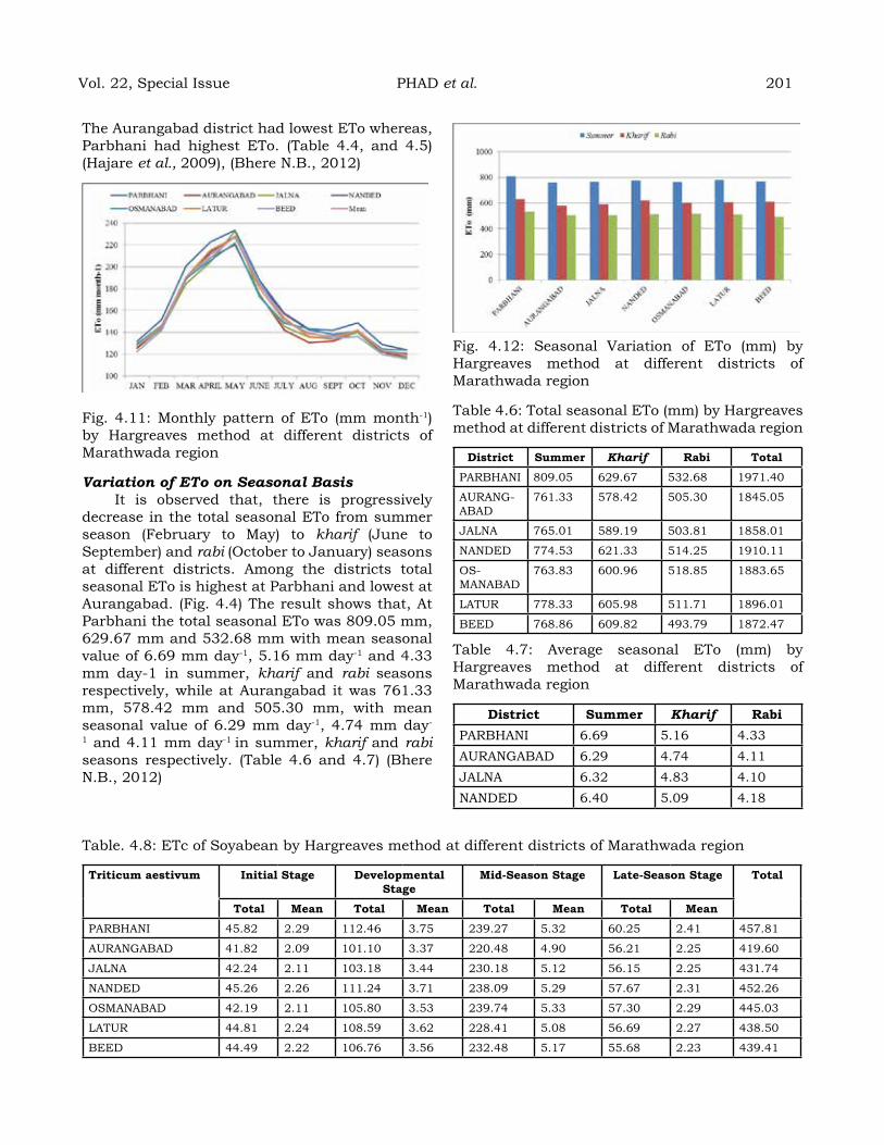
The Aurangabad district had lowest ETo whereas, Parbhani had highest ETo. (Table 4.4, and 4.5) (Hajare et al., 2009), (Bhere N.B., 2012)

Fig. 4.11: Monthly pattern of ETo (mm month-1) by Hargreaves method at different districts of Marathwada region

Variation of ETo on Seasonal BasisIt is observed that, there is progressively

decrease in the total seasonal ETo from summer season (February to May) to kharif (June to September) and rabi (October to January) seasons at different districts. Among the districts total seasonal ETo is highest at Parbhani and lowest at Aurangabad. (Fig. 4.4) The result shows that, At Parbhani the total seasonal ETo was 809.05 mm, 629.67 mm and 532.68 mm with mean seasonal value of 6.69 mm day-1, 5.16 mm day-1 and 4.33 mm day-1 in summer, kharif and rabi seasons respectively, while at Aurangabad it was 761.33 mm, 578.42 mm and 505.30 mm, with mean seasonal value of 6.29 mm day-1, 4.74 mm day-

1 and 4.11 mm day-1 in summer, kharif and rabi seasons respectively. (Table 4.6 and 4.7) (Bhere N.B., 2012)

Fig. 4.12: Seasonal Variation of ETo (mm) by Hargreaves method at different districts of Marathwada region

Table 4.6: Total seasonal ETo (mm) by Hargreaves method at different districts of Marathwada region

district Summer Kharif rabi total

PARBHANI 809.05 629.67 532.68 1971.40

AURANG-ABAD

761.33 578.42 505.30 1845.05

JALNA 765.01 589.19 503.81 1858.01

NANDED 774.53 621.33 514.25 1910.11

OS-MANABAD

763.83 600.96 518.85 1883.65

LATUR 778.33 605.98 511.71 1896.01

BEED 768.86 609.82 493.79 1872.47

Table 4.7: Average seasonal ETo (mm) by Hargreaves method at different districts of Marathwada region

district Summer Kharif rabiPARBHANI 6.69 5.16 4.33AURANGABAD 6.29 4.74 4.11JALNA 6.32 4.83 4.10NANDED 6.40 5.09 4.18

Table. 4.8: ETc of Soyabean by Hargreaves method at different districts of Marathwada region

triticum aestivum Initial Stage developmental Stage

Mid-Season Stage Late-Season Stage total

total Mean total Mean total Mean total Mean

PARBHANI 45.82 2.29 112.46 3.75 239.27 5.32 60.25 2.41 457.81

AURANGABAD 41.82 2.09 101.10 3.37 220.48 4.90 56.21 2.25 419.60

JALNA 42.24 2.11 103.18 3.44 230.18 5.12 56.15 2.25 431.74

NANDED 45.26 2.26 111.24 3.71 238.09 5.29 57.67 2.31 452.26

OSMANABAD 42.19 2.11 105.80 3.53 239.74 5.33 57.30 2.29 445.03

LATUR 44.81 2.24 108.59 3.62 228.41 5.08 56.69 2.27 438.50

BEED 44.49 2.22 106.76 3.56 232.48 5.17 55.68 2.23 439.41


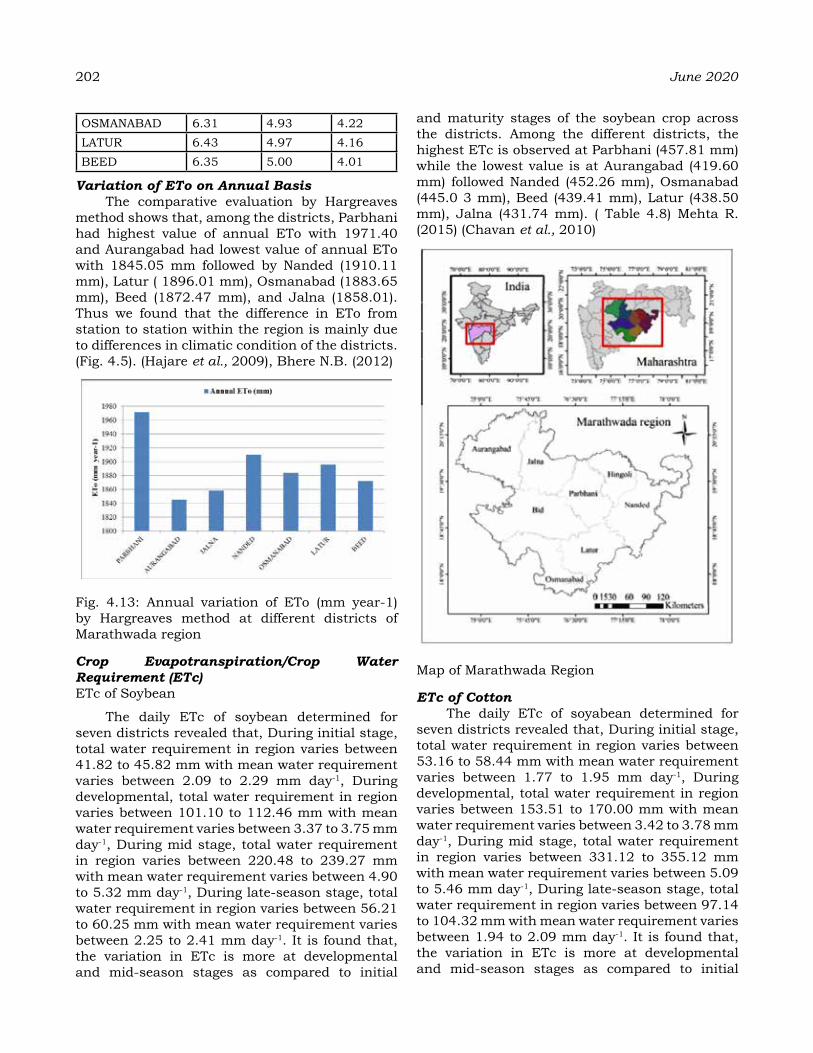
202 June 2020

OSMANABAD 6.31 4.93 4.22LATUR 6.43 4.97 4.16BEED 6.35 5.00 4.01

Variation of ETo on Annual BasisThe comparative evaluation by Hargreaves

method shows that, among the districts, Parbhani had highest value of annual ETo with 1971.40 and Aurangabad had lowest value of annual ETo with 1845.05 mm followed by Nanded (1910.11 mm), Latur ( 1896.01 mm), Osmanabad (1883.65 mm), Beed (1872.47 mm), and Jalna (1858.01). Thus we found that the difference in ETo from station to station within the region is mainly due to differences in climatic condition of the districts. (Fig. 4.5). (Hajare et al., 2009), Bhere N.B. (2012)

Fig. 4.13: Annual variation of ETo (mm year-1) by Hargreaves method at different districts of Marathwada region

Crop Evapotranspiration/Crop Water Requirement (ETc) ETc of Soybean

The daily ETc of soybean determined for seven districts revealed that, During initial stage, total water requirement in region varies between 41.82 to 45.82 mm with mean water requirement varies between 2.09 to 2.29 mm day-1, During developmental, total water requirement in region varies between 101.10 to 112.46 mm with mean water requirement varies between 3.37 to 3.75 mm day-1, During mid stage, total water requirement in region varies between 220.48 to 239.27 mm with mean water requirement varies between 4.90 to 5.32 mm day-1, During late-season stage, total water requirement in region varies between 56.21 to 60.25 mm with mean water requirement varies between 2.25 to 2.41 mm day-1. It is found that, the variation in ETc is more at developmental and mid-season stages as compared to initial

and maturity stages of the soybean crop across the districts. Among the different districts, the highest ETc is observed at Parbhani (457.81 mm) while the lowest value is at Aurangabad (419.60 mm) followed Nanded (452.26 mm), Osmanabad (445.0 3 mm), Beed (439.41 mm), Latur (438.50 mm), Jalna (431.74 mm). ( Table 4.8) Mehta R. (2015) (Chavan et al., 2010)

Map of Marathwada Region

ETc of CottonThe daily ETc of soyabean determined for

seven districts revealed that, During initial stage, total water requirement in region varies between 53.16 to 58.44 mm with mean water requirement varies between 1.77 to 1.95 mm day-1, During developmental, total water requirement in region varies between 153.51 to 170.00 mm with mean water requirement varies between 3.42 to 3.78 mm day-1, During mid stage, total water requirement in region varies between 331.12 to 355.12 mm with mean water requirement varies between 5.09 to 5.46 mm day-1, During late-season stage, total water requirement in region varies between 97.14 to 104.32 mm with mean water requirement varies between 1.94 to 2.09 mm day-1. It is found that, the variation in ETc is more at developmental and mid-season stages as compared to initial

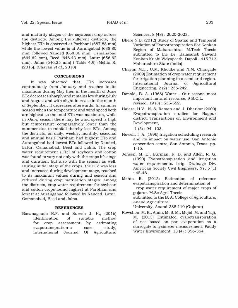
and maturity stages of the soyabean crop across the districts. Among the different districts, the highest ETc is observed at Parbhani (687.88 mm) while the lowest value is at Aurangabad (638.80 mm) followed Nanded (668.36 mm), Osmanabad (664.62 mm), Beed (648.43 mm), Latur (656.62 mm), Jalna (646.25 mm) ( Table 4.9) (Mehta R. (2015), (Chavan et al., 2010)

CoNCLuSIoNSIt was observed that, ETo increases

continuously from January and reaches to its maximum during May then in the month of June ETo decreases sharply and remains low during July and August and with slight increase in the month of September, it decreases afterwards. In summer season when the temperature and wind speed both are highest so the total ETo was maximum, while in kharif season there may be wind speed is high but temperature comparatively lower than the summer due to rainfall thereby less ETo. Among the districts, on daily, weekly, monthly, seasonal and annual basis Parbhani had highest ETo and Aurangabad had lowest ETo followed by Nanded, Latur, Osmanabad, Beed and Jalna. The crop water requirement (ETc) of soybean and cotton was found to vary not only with the crops it’s stage and duration, but also with the season as well. During initial stage of the crops, the ETc was less and increased during development stage, reached to its maximum values during mid season and reduced during crop maturation stages. Among the districts, crop water requirement for soybean and cotton crops found highest at Parbhani and lowest at Aurangabad followed by Nanded, Latur, Osmanabad, Beed and Jalna.

reFereNCeSBasanagouda R.F. and Suresh J. H., (2016)

Identification of suitable method for crop assessment by estimating evapotranspration-a case study, International Journal Of Agricultural

Sciences, 8 (48) : 2020-2023.Bhere N.B. (2012) Study of Spatial and Temporal

Variation of Evapotranspiration For Konkan Region of Maharashtra. M.Tech Thesis submitted to the Dr. Balasaheb Sawant Konkan Krishi Vidyapeeth. Dapoli - 415 712 Maharashtra State (India).

Chavan M.L., U.M. Khodke and N.M. Changade (2009) Estimation of crop water requirement for irrigation planning in a semi arid region. International Journal of Agricultural Engineering, 2 (2) : 236-242.

Donald, B. A. (1968) Water - Our second most important natural resource, 9 B.C.L. revised. 19 (3) : 535-552.

Hajare, H.V., N. S. Raman and J. Dharkar (2009) Evapotranspiration studies for Nagpur district. Transactions on Environment and Development,

1 (5) : 94 -103.Howell, T. A. (1996) Irrigation scheduling research

and its impact on water use. San Antonio convention centre, San Antonio, Texas. pp. 1-15.

Jensen, M. E., Burman, R. D. and Allen, R. G. (1990) Evapotranspiration and irrigation water requirements. Irrig. Drainage Div. American Society Civil Engineers, NY, 5 (1) : 45-48.

Mehta R. (2015) Estimation of reference evapotranspiration and determination of crop water requirement of major crops of gujarat. M.Sc Agri. Thesis submitted to the B. A. College of Agriculture, Anand Agricultural University, Anand-388 110 (Gujarat)

Rowshon, M. K., Amin, M. S. M., Mojid, M. and Yaji, M. (2013) Estimated evapotranspiration of rice based on pan evaporation as a surrogate to lysimeter measurement. Paddy Water Environment. 13 (4) : 356-364.


Spatial and temporal variation in the runoff potential and irrigation requirement of crops under changing climatic scenarios in the Western

vidarbha zone in Maharashtra1r.reJaNI*, 1K.v.rao, 1d. KaLYaNa SrINIvaS, 1K.SaMMI reddY, 1g.r. CharY, 1K.a.goPINath, 1M.oSMaN, 2r.S. Patode aNd 2M.B. Nagdeve

*Corresponding author, [email protected]/[email protected] Research Institute for Dryland Agriculture, Hyderabad

2AICRPDA Centre, Akola, Maharashtra

aBStraCtThe Western Vidarbha zone of Maharashtra has an average rainfall of 800 mm and dry spells are commonly experienced during July, August and September which coincides with the vegetative or reproductive stages of major rainfed crops. By providing one or two supplemental irrigation to these crops during critical growth stages can increase the yield considerably. Hence, estimation of runoff potential, its harvesting and optimal application is very important. In order to ensure long-term sustainability of crops, runoff potential and irrigation requirement of major crops were determined and analyzed for present and future scenarios. Higher rainfall was observed in few blocks of Amaravathi and Nagpur and lower in Buldana district. Considerable spatial variation in the irrigation requirement of major crops shows the need for site specific irrigation scheduling for this zone. A decreasing trend of rainfall in low rainfall areas and an increasing trend in high rainfall areas are predicted by 2050’s. Under climate change scenarios, an increase in the irrigation requirement of crops is expected for Buldana, Akola and Washim whereas a decreasing trend is projected for Nagpur, Wardha and parts of Amaravati and Yavatmal districts. The irrigation requirement predicted for kharif maize, pigeon pea, soybean, kharif sorghum and chickpea are not varying substantially at Akola by 2050’s. Hence, adoption of these crops in suitable soils could be one option for sustainable agriculture in future. In this region, runoff potential was relatively higher in Washim, Wardha and Nagpur districts and an increase in runoff potential predicted for major portion of the area by 2050’s showed higher potential for rainwater harvesting in future.

Keywords: Akola, climate change, crops, ensemble, irrigation requirement, Maharashtra, runoff

INtroduCtIoN An increase in temperature was observed in

India for the past one century with 0.21°C/10 years from 1970 onwards (Krishna Kumar, 2009). The climate change affects many sectors including agriculture. The annual per capita availability of water in India has reduced tremendously and is projected to decrease to 1140 m3 by 2050 (MOWR, 2008; Sneh Gangwar, 2013). The rise in surface temperature increases the evaporation rates, influences the precipitation, leads to extreme events and affects the soil moisture. In some drylands, increased evapotranspiration and decreased precipitation alongwith human activities resulted in desertification (IPCC, 2019). Indian agriculture is severely affected by climate change due to increased crop water requirement and decreased availability of water, particularly in drylands (INCCA, 2010; Behera et al., 2016). In rainfed areas, prolonged dry spells increases the water stress and reduces the growing period as well as crop productivity (IFPRI, 2009). Considerable increase in rainfall intensities are noted in many

areas in recent years shows increased potential for rainwater harvesting in those locations. According to fourth assessment report of IPCC, aver¬age river flow may increase in near the high latitudes, some wet trop¬ics and may reduce in dry tropics and dry areas at mid-latitudes (Nohara, 2006).

The rise in temperature increases the evaporation rates and finally influence the crop water requirement. The impact studies on crop water demand from Gujarat reported a gradual increase in water requirement for rabi and hot weather crops for the period of 2011-2099 (Parekh and Prajapati, 2013). Studies using PRECIS (explain PRECIS) data at Akola showed an increase in rainfall by 48.7%, PET by 13.1%, and sorghum yield by 183% by the end of the century (ICAR Network Annual Report, 2008-09). The adaptation strategies to cope with climate change impact on crops needs to be planned based on the site specific crop water demand and water availability (Kambale et al., 2015). The irrigation water requirement of potato in West Bengal is predicted to increase by 7 to 8% by 2020, and about 14 to


15% by 2050 (Chatterjee et al., 2012). Similarly, an increase in the rabi crop water requirement is predicted for the Vijayapura district in northern Karnataka (Rejani et al., 2016). It has been projected by various studies across the globe that the climate change is exacerbating available water for agriculture in future (Boonwichai, 2018).In this context, there is a need to adjust the site specific planning and optimal irrigation based on the continuously changing rainfall intensities and temperature patterns. Even though Vidarbha zone of Maharashtra has medium rainfall of around 800 mm, it experiences dry spells during July, August and September which coincides critical growth stages of major rainfed crops. The present study is aimed to assess the potential impacts of climate change on irrigation requirements of major crops and runoff potential availability in the Western Vidarbha zone of Maharashtra.

MethodoLogYStudy area

The study area, domain districts of Akola Centre in Western Vidarbha zone of Maharashtra covers an area of 62352 km² (Fig. 1). It lies between 19°15’ to 21°45’ N latitude and 75°45’ to 79°45’ E longitude.The elevation ranges from 100 to 1179 m above MSL and major portion of district is characterized by clayey, clay loam and loamy medium deep to very deep black soils (Source: NBSS & LUP). It is a semi-arid region consists of Akola, Washim, Buldana, Yavatmal, Amaravati, Wardha and part of Nagpur districts and it has an average annual rainfall of around 800 mm. Around 84% of the rainfall is received during southwest monsoon, and dry spells are experienced during July, August and September coincides with the vegetative or reproductive stages of major rainfed crops which in turn affects the crop yield drastically. The major crops grown include cotton, soybean, green gram, pigeon pea, sorghum and rabi chickpea. By providing one or two supplemental irrigation to these rainfed crops during critical growth stages or prolonged dry spells can increase the crop yield considerably. Hence, estimation of runoff potential available for harvesting and the irrigation requirement of crops for optimal application are very important. With changing climatic scenarios, to meet the food and water demand for the growing population in future is a great challenge. Therefore, it is necessary to improve the water resources management particularly for agriculture by adopting the optimal irrigation schedule instead of flooding the whole field.

Fig. 1: Location map of the study area

Irrigation requirement of cropsThe crop water requirement was estimated

for major crops which includes cotton, soybean, green gram, pigeon pea, sorghum and rabi chickpea. Though FAO Penman-Monteith method is the standard method for ETo calculation (Allen et al., 1998), based on data availability for future scenarios, Hargreaves and Samani (1985) method was used. The crop evapotranspiration (ETc) and GIR were calculated the using the Eqn (1 & 2).

ETC = kc ET0 (1)

where kc is the crop coefficient depends on the crop growth stages

(2)

where GIR = gross irrigation requirement (mm) ; Re = effective rainfall (mm) ; ηp= project efficiency (application efficiency x conveyance efficiency x field canal efficiency). The effective rainfall is estimated from 10 day rainfall using empirical Eqns (3 & 4)

Pef = P (41.7-0.2P) /41.7 for P≤83 (3)

Pef = 41.7+0.1PforP>83 (4)

where Pef= 10 days effective rainfall (mm) and P = 10 days rainfall (mm)

Modeling studies under changing climatic scenarios

The runoff potential availability and irrigation requirement of major crops were determined and analyzed for present scenario as well as for future

Vol. 22, Special Issue REJANI et al. 205

206 June 2020

scenarios, namely, 2020’s (2010 to 2039) and 2050’s (2040 to 2069). The IMD data and ensemble data of (explain CMIP) CMIP 5 corresponding to three emission scenarios namely, (explain RCP) RCP 2.6, RCP 4.5 and RCP 6.0 were used. The selected area is prone to prolonged dry spells, delayed and deficient monsoon. Since this area is characterized by medium rainfall and runoff potential, in-situ moisture conservation and water harvesting can help to recharge the groundwater and supplement the irrigation requirement. Most of the area is covered by crops followed by forest (Fig. 1). The spatial and temporal variability of rainfall, runoff potential and irrigation requirement of crops were analyzed during baseline period, 2020’s and 2050’s under different emission scenarios. Calibrated and validated SWAT model was used for estimating the runoff potential for the study area under different climate change scenarios. The variability in the irrigation demand and the runoff potential availability in the near future will help in the sustainable planning of water harvesting structures.

reSuLtS aNd dISCuSSIoNVariability in the ET and irrigation requirement of crops

Site specific irrigation requirement of major crops was determined for Western Vidarbha zone of Maharashtra for the period 1951-2013 using Hargreaves method coupled with GIS. Considerable spatial variation in the irrigation requirement of crops like soybean, greengram, kharif sorghum, rabisorghum, pigeonpea, cotton and chickpea are noted at Western Vidarbha zone. Irrigation requirement of major crops was more in the blocks of Buldana, Akola and Yavatmal districts (Fig. 2a-b). The need for irrigation is more in these districts due to the less rainfall availability in kharif season and the scope for rainwater harvesting and supplemental irrigation is also relatively low due to low runoff potential (Fig. 4a-b) compared to other districts. Adoption of in-situ moisture conservation practice and mulching are of prime importance in this area. An increase in the in the irrigation requirement of major crops are noted in most of the blocks over the years (1951 to 2013) (Fig. 3a-b). Considerable spatial variation in the irrigation requirement of major crops shows the need for site specific irrigation scheduling for Western Vidarbha zone.

Fig. 2a-b. Variation in the irrigation requirement of crops (1951-2013) at Vidarbha

Fig. 3a-b: Spatial variation in the irrigation requirement of cotton at Western Vidarbha zone of Maharashtra during (i) 1972-1992 and (ii) 1993-2013 w.r.t 1951-1971

Fig. 4a-b. Spatial variation of rainfall and runoff at Vidarbha

Variability in the irrigation requirement of crops under climate change scenarios

The maximum temperature rises up to 45.3 to 46.7 0C in and minimum temperature declines below 5 to 6.40C in different districts. Under changing climatic scenarios, a decrease of rainfall in low rainfall areas and increase of rainfall under high rainfall areas are noted by 2050’s. Similarly, an increase of minimum and maximum temperatures also noted under all scenarios. The evapotranspiration under changing climatic scenarios were estimated using ensemble data with Hargreaves method and GIS. Considerable spatial variation in the irrigation requirement of different crops over the years was observed during 2020’s and 2050’s under different emission scenarios with respect to base line period (Table 1).

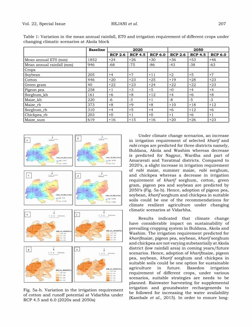
Fig. 5a-h. Variation in the irrigation requirement of cotton and runoff potential at Vidarbha under RCP 4.5 and 6.0 (2020s and 2050s)

Under climate change scenarios, an increase in irrigation requirement of selected kharif and rabi crops are predicted for three districts namely, Buldana, Akola and Washim whereas decrease is predicted for Nagpur, Wardha and part of Amaravati and Yavatmal districts. Compared to 2020’s, a slight increase in irrigation requirement of rabi maize, summer maize, rabi sorghum, and chickpea whereas a decrease in irrigation requirement of kharif sorghum, cotton, green gram, pigeon pea and soybean are predicted by 2050’s (Fig. 5a-h). Hence, adoption of pigeon pea, soybean, kharif sorghum and chickpea in suitable soils could be one of the recommendations for climate resilient agriculture under changing climatic scenarios at Vidarbha.

Results indicated that climate change have considerable impact on sustainability of prevailing cropping system in Buldana, Akola and Washim. The irrigation requirement predicted for kharifmaize, pigeon pea, soybean, kharif sorghum and chickpea are not varying substantially at Akola district (low rainfall area) in coming years/future scenarios. Hence, adoption of kharifmaize, pigeon pea, soybean, kharif sorghum and chickpea in suitable soils could be one option for sustainable agriculture in future. Basedon irrigation requirement of different crops, under various scenarios, suitable strategies are needs to be planned. Rainwater harvesting for supplemental irrigation and groundwater rechargeneeds to be followed for increasing the water availability (Kambale et al., 2015). In order to ensure long-

Table 1: Variation in the mean annual rainfall, ET0 and irrigation requirement of different crops under changing climatic scenarios at Akola block

Baseline 2020 2050rCP 2.6 rCP 4.5 rCP 6.0 rCP 2.6 rCP 4.5 rCP 6.0

Mean annual ET0 (mm) 1852 +24 +26 +30 +36 +53 +46Mean annual rainfall (mm) 946 -68 -75 -86 -43 -38 -63CropsSoybean 205 +4 +7 +11 +2 +5 +7Cotton 446 +20 +23 +25 +19 +28 +23Green gram 40 +22 +23 +24 +22 +22 +23Pigeon pea 258 +1 +3 +5 +0 +4 +4Sorghum_kh 161 +6 +8 +12 +4 +6 +8Maize_kh 220 -6 -3 +1 -8 -5 -3Maize_rb 373 +8 +9 +8 +10 +18 +12Sorghum_rb 310 +4 +5 +4 +6 +12 +6Chickpea_rb 203 +0 +1 +0 +1 +6 +1Maize_sum 619 +16 +15 +16 +20 +26 +23


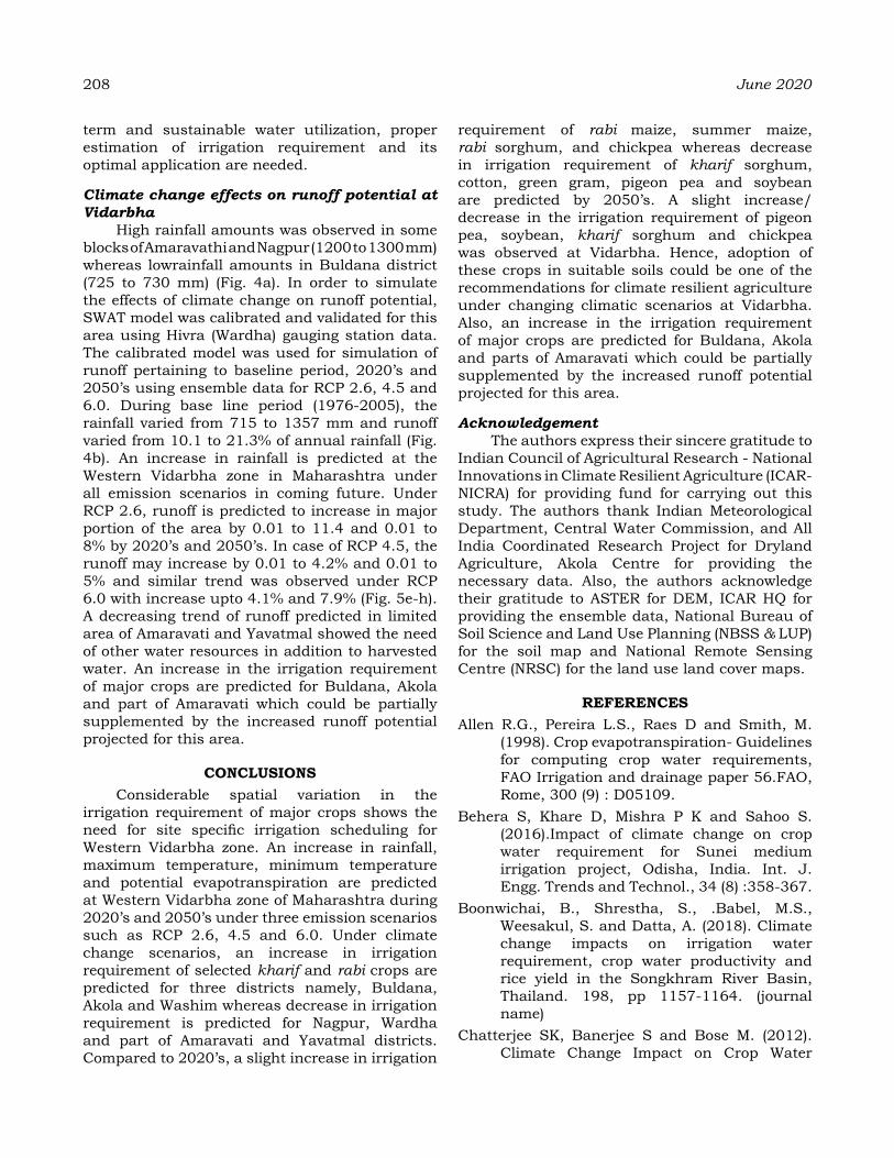
208 June 2020

term and sustainable water utilization, proper estimation of irrigation requirement and its optimal application are needed.

Climate change effects on runoff potential at Vidarbha

High rainfall amounts was observed in some blocks of Amaravathi and Nagpur (1200 to 1300 mm) whereas lowrainfall amounts in Buldana district (725 to 730 mm) (Fig. 4a). In order to simulate the effects of climate change on runoff potential, SWAT model was calibrated and validated for this area using Hivra (Wardha) gauging station data. The calibrated model was used for simulation of runoff pertaining to baseline period, 2020’s and 2050’s using ensemble data for RCP 2.6, 4.5 and 6.0. During base line period (1976-2005), the rainfall varied from 715 to 1357 mm and runoff varied from 10.1 to 21.3% of annual rainfall (Fig. 4b). An increase in rainfall is predicted at the Western Vidarbha zone in Maharashtra under all emission scenarios in coming future. Under RCP 2.6, runoff is predicted to increase in major portion of the area by 0.01 to 11.4 and 0.01 to 8% by 2020’s and 2050’s. In case of RCP 4.5, the runoff may increase by 0.01 to 4.2% and 0.01 to 5% and similar trend was observed under RCP 6.0 with increase upto 4.1% and 7.9% (Fig. 5e-h). A decreasing trend of runoff predicted in limited area of Amaravati and Yavatmal showed the need of other water resources in addition to harvested water. An increase in the irrigation requirement of major crops are predicted for Buldana, Akola and part of Amaravati which could be partially supplemented by the increased runoff potential projected for this area.

CoNCLuSIoNSConsiderable spatial variation in the

irrigation requirement of major crops shows the need for site specific irrigation scheduling for Western Vidarbha zone. An increase in rainfall, maximum temperature, minimum temperature and potential evapotranspiration are predicted at Western Vidarbha zone of Maharashtra during 2020’s and 2050’s under three emission scenarios such as RCP 2.6, 4.5 and 6.0. Under climate change scenarios, an increase in irrigation requirement of selected kharif and rabi crops are predicted for three districts namely, Buldana, Akola and Washim whereas decrease in irrigation requirement is predicted for Nagpur, Wardha and part of Amaravati and Yavatmal districts. Compared to 2020’s, a slight increase in irrigation

requirement of rabi maize, summer maize, rabi sorghum, and chickpea whereas decrease in irrigation requirement of kharif sorghum, cotton, green gram, pigeon pea and soybean are predicted by 2050’s. A slight increase/decrease in the irrigation requirement of pigeon pea, soybean, kharif sorghum and chickpea was observed at Vidarbha. Hence, adoption of these crops in suitable soils could be one of the recommendations for climate resilient agriculture under changing climatic scenarios at Vidarbha. Also, an increase in the irrigation requirement of major crops are predicted for Buldana, Akola and parts of Amaravati which could be partially supplemented by the increased runoff potential projected for this area.

AcknowledgementThe authors express their sincere gratitude to

Indian Council of Agricultural Research - National Innovations in Climate Resilient Agriculture (ICAR- NICRA) for providing fund for carrying out this study. The authors thank Indian Meteorological Department, Central Water Commission, and All India Coordinated Research Project for Dryland Agriculture, Akola Centre for providing the necessary data. Also, the authors acknowledge their gratitude to ASTER for DEM, ICAR HQ for providing the ensemble data, National Bureau of Soil Science and Land Use Planning (NBSS & LUP) for the soil map and National Remote Sensing Centre (NRSC) for the land use land cover maps.

reFereNCeSAllen R.G., Pereira L.S., Raes D and Smith, M.

(1998). Crop evapotranspiration- Guidelines for computing crop water requirements, FAO Irrigation and drainage paper 56.FAO, Rome, 300 (9) : D05109.

Behera S, Khare D, Mishra P K and Sahoo S. (2016).Impact of climate change on crop water requirement for Sunei medium irrigation project, Odisha, India. Int. J. Engg. Trends and Technol., 34 (8) :358-367.

Boonwichai, B., Shrestha, S., .Babel, M.S., Weesakul, S. and Datta, A. (2018). Climate change impacts on irrigation water requirement, crop water productivity and rice yield in the Songkhram River Basin, Thailand. 198, pp 1157-1164. (journal name)

Chatterjee SK, Banerjee S and Bose M. (2012). Climate Change Impact on Crop Water

Requirement in Ganga River Basin, West Bengal, India. In 3rd International Conference on Biology, Environment and Chemistry, 46:17-20.

Hargreaves GH and Samani ZA. (1985). Reference crop evapotranspiration from temperature.Applied Engg. Agric., 1 (2) : 96-99.

ICAR Network Annual Report. (2008-09). ICAR Network Project on Impact, Adaptation and Vulnerability of Indian Agriculture to Climate Change, ICAR CRIDA, p.130

IFPRI. (2009). Climate Change – Impact on Agriculture and Costs of Adaptation, Food Policy. Report International Food Policy Research Institute, Washington, D.C., U.S.A., pp.30.

INCCA. (2010). Indian Network for Climate Change Assessment, Climate Change and India: A 4x4 Assessment, Ministry of Environment and Forests, Government of India.

IPCC. (2007). Climate change 2007: The physical science basis. Contribution of Working Group I to the fourth assessment report of the Inter governmental Panel on Climate Change. Cambridge University Press, Cambridge, United Kingdom, New York, NY, USA.

IPCC. (2019). Summary for Policymakers. In: Climate Change and Land: an IPCC Special report on climate change, desertification, land degradation, sustainable land management, food security, and greenhouse gas fluxes in terrestrial ecosystems [P.R. Shukla et al., (eds.) ]. In press.

Kambale JB, Singh DK and Sarangi A. (2015). Strategies for climate change impacts on irrigated crops in National Capital Region of

India. J. Applied and Natural Sci., 7 (1) : 388-393.

Krishna Kumar. (2009). Impact of climate change on India’s monsoon climate and development of high resolution climate change scenarios for India. Presented at Ministry of Environment and Forest (MoEF), New Delhi on October 14, 2009 (http: moef.nic.in)

MOWR (2008). Ministry of Water Resources, Report of Sub-Committee on Policy and Institutional Framework. National Water Mission under National Action Plan on Climate Change. Comprehensive Mission Document, Volume - II, Ministry of Water Resources, Government of India, New Delhi.http://wrmin.nic.in/writereaddata/nwm28756944786.pdf

Nohara, D. (2006). Impact of climate change on river discharge projected by multi-model ensemble. J. Hydrometeorol., 7 (5), 1076–89.

Parekh and Prajapati (2013). Climate change impacts on crop water requirement for sukhi reservoir project. Int. J. Innovative Res. Sci., Engg and Technol., 9 (5), pp. 4685-4692

Rejani, R. Rao, K.V. Shirahatti, M.S. Surakod, V.S. Yogitha, P. Chary, G.R. Gopinath, K.A. Osman, M. Sammi Reddy, Kand Srinivasa Rao, Ch. (2016). Irrigation requirement of crops under changing climatic scenarios in a semi-arid region of Northern Karnataka.Indian J. Dry land Agric. Res. & Dev., 31 (2) : 51-60.

Sneh Gangwar. (2013). Water Resource of India: From Distribution to Management. Int. J. Information and Computation Technol., 3 (8) : 845-850.


Mapping of groundwater quality for suitability of climate resilient farming in the eastern agro-climatic zone of haryana, India

raM PraKaSh1*, SaNJaY KuMar2, SatYavaN1 aNd SureNder SINgh3

1Department of Soil Science, 2Department of Soil and Water Engineering3Department of Agril Meteorology, CCS Haryana Agricultural University, Hisar, India

*Corresponding author E-mail: [email protected]

aBStraCtChanges in global climate are expected to affect the hydrological cycle, altering surface - water levels and groundwater recharge to aquifers with various other associated impacts on the natural ecosystems including groundwater quality. Climate change likely to affect rainfall patterns, consequently managing water quality very difficult with much uncertainty. A survey experiment was conducted at different villages of Eastern Agro-climatic Zone of Haryana during 2015-16 & 2016-17 to appraise the water quality for the irrigation use to attain sustainable crop production. In the preceding decade (2006-15) generally deficit to scanty rainfall trend was observed in the monsoon season, hence, almost no natural recharging of the ground water in the region was there. In order to assess the ground water quality, a total 530 water samples were collected and analyzed for various chemical properties like EC, pH, cations (Na+, K, Ca2+ and Mg2+) and anions (Cl-, SO4

2-, CO32- and HCO3

-) by standard procedure. Irrigation indices viz., Sodium adsorption ratio (SAR), Residual sodium carbonate (RSC), was calculated for these samples. The EC, pH, RSC and SAR in groundwater ranged from 0.30-8.25 (d S m-1), 7.01-9.80, 0.00-6.90 (mel-1) and 2.55-27.67 (mmoll-1) 1/2, respectively. The trend among the average ionic concentration of cations and anions are Na+ > Mg2+ > Ca2+ > K+ and Cl- > SO4

2- > HCO3- > CO3

2. According to AICRP classification, 47.2, 12.1, 7.7, 11.3, 13.0 and 8.87% of the samples were of good, marginally saline, high SAR saline, marginally alkali, alkali and highly alkali, respectively. To investigate the ionic toxicity of the region, derived parameters such as magnesium hazard (MH), soluble sodium percentage (SSP), magnesium adsorption ratio, permeability index (PI) and Kelly’s ratio (KR) were calculated. According to the existence of these parameters, groundwater found to be moderately suitable for irrigation purpose for the various crops in the agro-climatic zone.

Keywords: Groundwater, Permeability Index, Climate Resilient Farming, Rainfall Trend, Agro-climatic Zone.

INtroduCtIoN

Climate change may be felt in the aquifers at hydro chemical and hydrodynamic levels. The change in temperature, the increase of CO2 dissolved in rainwater and the change in rainfall pattern can promote a greater dissolution or precipitation of carbonate minerals. Extreme drought conditions increase the residence time of groundwater, with consequences on water quality by increasing the reaction time of the water with rocks. In the past few decades, there has been unusual rise in the fresh water condition because of increase in human population, urbanization, industrialization, and intensive agricultural activities. Geographical and temporal classification of water quality and its suitability for drinking and irrigation using Geospatial Information Systems (GIS), Water Quality Index (WQI) and other Information and Communication Technology (ICT) etc have been reported by many researchers (Anurag et al., 2009; Singh et al., 2009; Singh et

al., 2012; Mehta and Pandey, 2015). Due to lack of surface water which is also caused by pollution, industrial growth, urbanization and because of the notion that groundwater is polluted free of charge, most of India’s population relies on groundwater for domestic, industrial and agricultural use (Raju et al., 2011). Groundwater quality assessment is important not only for the present generation but also for the future generation. The underground resources of alluvial plains in the Indo Gangetic basin show a valid and quantitative basis over time (Haritash, et al., 2008). So regular observation of groundwater quality is necessary which affects the fittingness of water for climate resilient farming. In modern times, water has critical importance for the economic growth of all contemporary societies (Yadagiri, et al., 2015). Water resources on the earth have been categorized in different types based on their availability and suitability for various purposes. The reduction of global surface water resources due to overuse and contamination with various chemical and biological sources


is adding huge force on groundwater resources (Singh, et al., 2006). Presently groundwater is the most important source of irrigation in India, thus deserving considerable attention for use in a sustainable way quantitatively and qualitatively. Evaluation of groundwater quality for irrigation is importance for arid and semi-arid regions of the planet in general and to developing countries like India in particular. Good quality water is needed to feed the rapidly increasing human population, addition of irrigated farming and growth of industrial settings (Toumi, et al., 2015). The quality of water can be evaluated by its aesthetic, physical, chemical and biological properties, which get influenced by agricultural, industrial and anthropogenic uses. The spatial variations are due to its natural hydrogeological setting, while the temporal variability in a particular area is often assigned to anthropogenic reasons (Adhikari, et al., 2012). Limited freshwater availability and increasing demand for food are making even marginal and poor quality waters, an important source for irrigation. The main complexity of irrigating the crop with poor quality water is not really the short-term effect rather the long-term changes on soil properties that might critically amend its fertility (Cucci et al., 2013). Out of total cultivated area of 3.62 mha, 1.65 mha is irrigated with tube wells often containing water of doubtful quality in Haryana state, 45% of the water is of good condition and 55% is either saline or sodic in nature, the exploitation of groundwater resources is causing a decline in the water table and is a cause of great concern in some parts of Gujarat, Rajasthan, Haryana, Punjab, Andhra Pradesh, Maharashtra and Tamil Nadu. Degradation can be delayed to some extent by improving the re-use of rainwater and surface water used for the efficient distribution of the water injection techniques. Water quality data is essential for the implementation of responsible water quality regulations for characterizing and remediating contamination and for the protection of the health of humans and the ecosystem. Regular monitoring of groundwater resources thus, plays a key role in sustainable management of water resources. The association of chloride/sulphate and/or carbonate/bicarbonate excess of sodium ions characterizes the water as saline or alkaline. Subsequently, the soils develop salinity or sodic problems when irrigated with such type of water; more particularly in absence of drainage and soil management practices. The current study is being done determine the vulnerability

of groundwater vis-à-vis its fitness for irrigation in Kaithal district representing Eastern agro-climatic zone of Haryana state.

MaterIaL aNd MethodSStudy area

A survey experiment was conducted at different villages of Kaithal, district representing Eastern agro-climatic zone of Haryana during 2015-16 and 2016-17 to assess the quality of underground water for irrigation for crops. Kaithal district is located between 29o31’- 30o12’ North latitudes and 76o10’- 76o42’ East longitudes in the eastern agro-climatic zone of Haryana, India. Kaithal district is divided into 6 blocks namely Guhla, Kaithal, Kalayat, Rajound, Siwan and Pundari. A map of the study area is given in Fig. 1. The climate of the district has been characterized as semiarid and very hot very hot in summer and cold in winter. The district in the agro-climatic zone mainly receives highly erratic rainfall of 380 mm during SW monsoon. The rainfall over the past decade (2006-15), periods of monsoon seasons was mostly deficit and scanty ranging from -23 per cent (2011) to -71 per cent (2014) except in the year 2010, where it was normal (13%) against normal rainfall of 480 mm; thus, almost no natural reviving of ground water in this area (Table 1).

Fig. 1: The location Map of Kaithal district representing its block and villages

Table 1: Monsoon seasonal rainfall during the preceding decade (2006-16) in the study domain

Sr. No. Monsoonal year (s) Rainfall deviation (%)

1 2006 -522 2007 -52

Vol. 22, Special Issue PRAKASH et al. 211

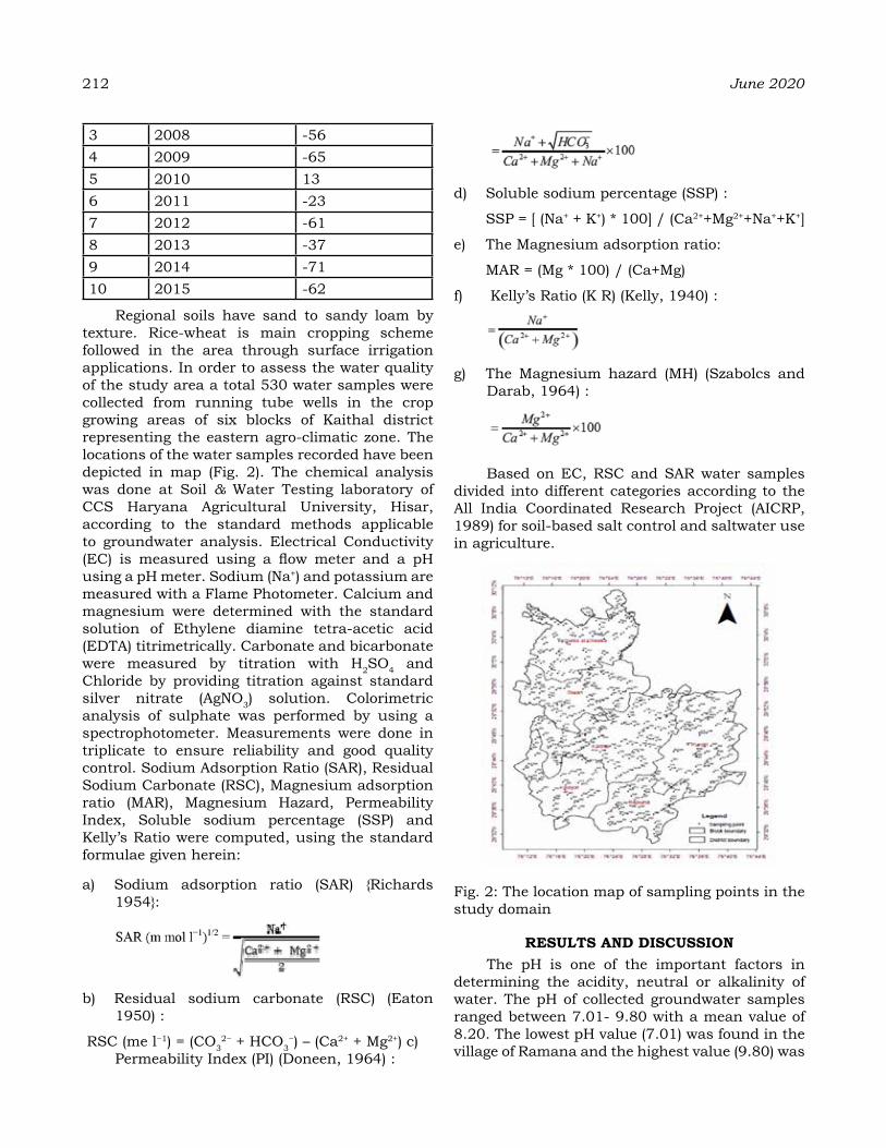
212 June 2020

3 2008 -564 2009 -655 2010 136 2011 -237 2012 -618 2013 -379 2014 -7110 2015 -62

Regional soils have sand to sandy loam by texture. Rice-wheat is main cropping scheme followed in the area through surface irrigation applications. In order to assess the water quality of the study area a total 530 water samples were collected from running tube wells in the crop growing areas of six blocks of Kaithal district representing the eastern agro-climatic zone. The locations of the water samples recorded have been depicted in map (Fig. 2). The chemical analysis was done at Soil & Water Testing laboratory of CCS Haryana Agricultural University, Hisar, according to the standard methods applicable to groundwater analysis. Electrical Conductivity (EC) is measured using a flow meter and a pH using a pH meter. Sodium (Na+) and potassium are measured with a Flame Photometer. Calcium and magnesium were determined with the standard solution of Ethylene diamine tetra-acetic acid (EDTA) titrimetrically. Carbonate and bicarbonate were measured by titration with H2SO4 and Chloride by providing titration against standard silver nitrate (AgNO3) solution. Colorimetric analysis of sulphate was performed by using a spectrophotometer. Measurements were done in triplicate to ensure reliability and good quality control. Sodium Adsorption Ratio (SAR), Residual Sodium Carbonate (RSC), Magnesium adsorption ratio (MAR), Magnesium Hazard, Permeability Index, Soluble sodium percentage (SSP) and Kelly’s Ratio were computed, using the standard formulae given herein:

a) Sodium adsorption ratio (SAR) {Richards 1954}:

b) Residual sodium carbonate (RSC) (Eaton 1950) :

RSC (me l−1) = (CO32− + HCO3

−) – (Ca2+ + Mg2+) c) Permeability Index (PI) (Doneen, 1964) :

d) Soluble sodium percentage (SSP) :

SSP = [ (Na+ + K+) * 100] / (Ca2++Mg2++Na++K+]

e) The Magnesium adsorption ratio:

MAR = (Mg * 100) / (Ca+Mg)

f) Kelly’s Ratio (K R) (Kelly, 1940) :

g) The Magnesium hazard (MH) (Szabolcs and Darab, 1964) :

Based on EC, RSC and SAR water samples divided into different categories according to the All India Coordinated Research Project (AICRP, 1989) for soil-based salt control and saltwater use in agriculture.

Fig. 2: The location map of sampling points in the study domain

reSuLtS aNd dISCuSSIoNThe pH is one of the important factors in

determining the acidity, neutral or alkalinity of water. The pH of collected groundwater samples ranged between 7.01- 9.80 with a mean value of 8.20. The lowest pH value (7.01) was found in the village of Ramana and the highest value (9.80) was

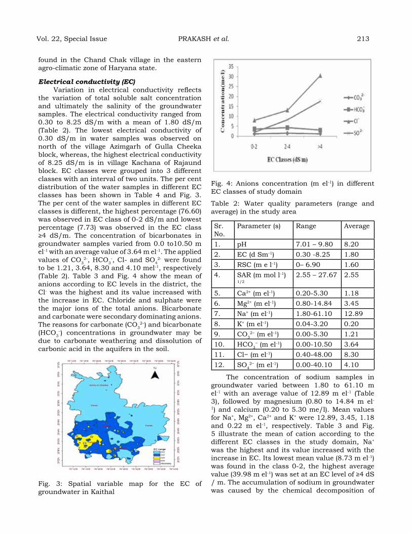
found in the Chand Chak village in the eastern agro-climatic zone of Haryana state.

Electrical conductivity (EC) Variation in electrical conductivity reflects

the variation of total soluble salt concentration and ultimately the salinity of the groundwater samples. The electrical conductivity ranged from 0.30 to 8.25 dS/m with a mean of 1.80 dS/m (Table 2). The lowest electrical conductivity of 0.30 dS/m in water samples was observed on north of the village Azimgarh of Gulla Cheeka block, whereas, the highest electrical conductivity of 8.25 dS/m is in village Kachana of Rajaund block. EC classes were grouped into 3 different classes with an interval of two units. The per cent distribution of the water samples in different EC classes has been shown in Table 4 and Fig. 3. The per cent of the water samples in different EC classes is different, the highest percentage (76.60) was observed in EC class of 0-2 dS/m and lowest percentage (7.73) was observed in the EC class ≥4 dS/m. The concentration of bicarbonates in groundwater samples varied from 0.0 to10.50 m el-1 with an average value of 3.64 m el-1. The applied values of CO3

2-, HCO3-, Cl- and SO4

2- were found to be 1.21, 3.64, 8.30 and 4.10 mel-1, respectively (Table 2). Table 3 and Fig. 4 show the mean of anions according to EC levels in the district, the Cl- was the highest and its value increased with the increase in EC. Chloride and sulphate were the major ions of the total anions. Bicarbonate and carbonate were secondary dominating anions. The reasons for carbonate (CO3

2–) and bicarbonate (HCO3

–) concentrations in groundwater may be due to carbonate weathering and dissolution of carbonic acid in the aquifers in the soil.

Fig. 3: Spatial variable map for the EC of groundwater in Kaithal

Fig. 4: Anions concentration (m el-1) in different EC classes of study domain

Table 2: Water quality parameters (range and average) in the study area

Sr. No.

Parameter (s) Range Average

1. pH 7.01 – 9.80 8.202. EC (d Sm-1) 0.30 -8.25 1.803. RSC (m e l-1) 0– 6.90 1.604. SAR (m mol l-1)

1/22.55 – 27.67 2.55

5. Ca2+ (m el-1) 0.20-5.30 1.186. Mg2+ (m el-1) 0.80-14.84 3.457. Na+ (m el-1) 1.80-61.10 12.898. K+ (m el-1) 0.04-3.20 0.209. CO3

2− (m el-1) 0.00-5.30 1.2110. HCO3

− (m el-1) 0.00-10.50 3.6411. Cl− (m el-1) 0.40-48.00 8.3012. SO4

2− (m el-1) 0.00-40.10 4.10

The concentration of sodium samples in groundwater varied between 1.80 to 61.10 m el-1 with an average value of 12.89 m el-1 (Table 3), followed by magnesium (0.80 to 14.84 m el-1) and calcium (0.20 to 5.30 me/l). Mean values for Na+, Mg2+, Ca2+ and K+ were 12.89, 3.45, 1.18 and 0.22 m el-1, respectively. Table 3 and Fig. 5 illustrate the mean of cation according to the different EC classes in the study domain, Na+ was the highest and its value increased with the increase in EC. Its lowest mean value (8.73 m el-1) was found in the class 0-2, the highest average value (39.98 m el-1) was set at an EC level of ≥4 dS / m. The accumulation of sodium in groundwater was caused by the chemical decomposition of


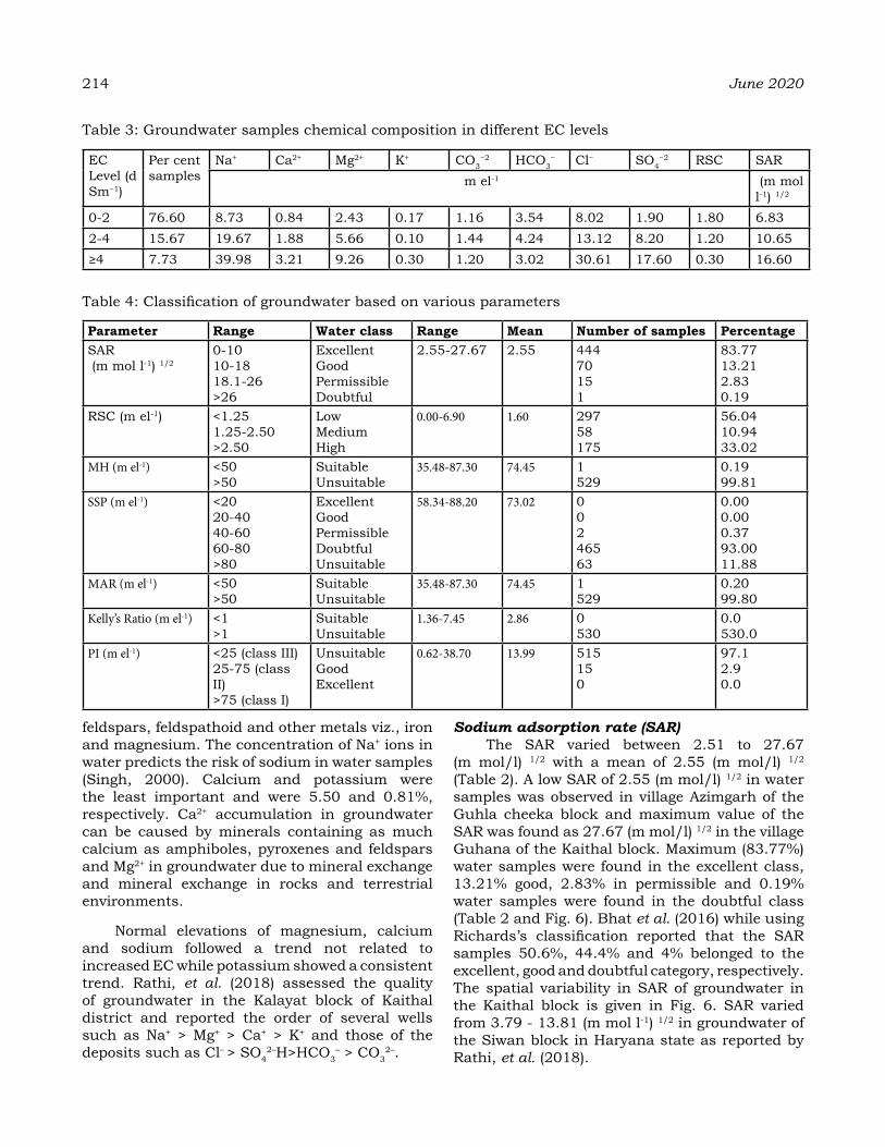
214 June 2020

feldspars, feldspathoid and other metals viz., iron and magnesium. The concentration of Na+ ions in water predicts the risk of sodium in water samples (Singh, 2000). Calcium and potassium were the least important and were 5.50 and 0.81%, respectively. Ca2+ accumulation in groundwater can be caused by minerals containing as much calcium as amphiboles, pyroxenes and feldspars and Mg2+ in groundwater due to mineral exchange and mineral exchange in rocks and terrestrial environments.

Normal elevations of magnesium, calcium and sodium followed a trend not related to increased EC while potassium showed a consistent trend. Rathi, et al. (2018) assessed the quality of groundwater in the Kalayat block of Kaithal district and reported the order of several wells such as Na+ > Mg+ > Ca+ > K+ and those of the deposits such as Cl– > SO4

2–H>HCO3– > CO3

2–.

Sodium adsorption rate (SAR) The SAR varied between 2.51 to 27.67

(m mol/l) 1/2 with a mean of 2.55 (m mol/l) 1/2 (Table 2). A low SAR of 2.55 (m mol/l) 1/2 in water samples was observed in village Azimgarh of the Guhla cheeka block and maximum value of the SAR was found as 27.67 (m mol/l) 1/2 in the village Guhana of the Kaithal block. Maximum (83.77%) water samples were found in the excellent class, 13.21% good, 2.83% in permissible and 0.19% water samples were found in the doubtful class (Table 2 and Fig. 6). Bhat et al. (2016) while using Richards’s classification reported that the SAR samples 50.6%, 44.4% and 4% belonged to the excellent, good and doubtful category, respectively. The spatial variability in SAR of groundwater in the Kaithal block is given in Fig. 6. SAR varied from 3.79 - 13.81 (m mol l-1) 1/2 in groundwater of the Siwan block in Haryana state as reported by Rathi, et al. (2018).

Table 3: Groundwater samples chemical composition in different EC levels

EC Level (d Sm−1)

Per cent samples

Na+ Ca2+ Mg2+ K+ CO3−2 HCO3

− Cl− SO4−2 RSC SAR

m el-1 (m mol l-1) 1/2

0-2 76.60 8.73 0.84 2.43 0.17 1.16 3.54 8.02 1.90 1.80 6.832-4 15.67 19.67 1.88 5.66 0.10 1.44 4.24 13.12 8.20 1.20 10.65≥4 7.73 39.98 3.21 9.26 0.30 1.20 3.02 30.61 17.60 0.30 16.60

Table 4: Classification of groundwater based on various parameters

Parameter range Water class range Mean Number of samples PercentageSAR (m mol l-1) 1/2

0-1010-1818.1-26>26

ExcellentGoodPermissibleDoubtful

2.55-27.67 2.55 44470151

83.7713.212.830.19

RSC (m el-1) <1.251.25-2.50>2.50

LowMediumHigh

0.00-6.90 1.60 29758175

56.0410.9433.02

MH (m el-1) <50>50

SuitableUnsuitable

35.48-87.30 74.45 1529

0.1999.81

SSP (m el-1) <2020-4040-6060-80>80

ExcellentGoodPermissibleDoubtfulUnsuitable

58.34-88.20 73.02 00246563

0.000.000.3793.0011.88

MAR (m el-1) <50>50

SuitableUnsuitable

35.48-87.30 74.45 1529

0.2099.80

Kelly’s Ratio (m el-1) <1>1

SuitableUnsuitable

1.36-7.45 2.86 0530

0.0530.0

PI (m el-1) <25 (class III) 25-75 (class II) >75 (class I)

UnsuitableGoodExcellent

0.62-38.70 13.99 515150

97.12.90.0

Fig. 5: Cations (Ca, Mg, Na, K) conc (m el-1) in different EC classes of study domain

Fig. 6: The spatial variable map of SAR of groundwater of study domain

Residual Sodium Carbonate (RSC) Residual sodium carbonate (RSC) for

agricultural purposes is usually used to assess the harmful effect of carbonate and bicarbonate in the water quality. The residual sodium carbonate was recorded between 0.00 to 6.90 m el-1 with a mean of 1.60 m el-1 (Table 2). The highest RSC of 9.40 m el-1 in water samples was observed in the Tik village of Kaithal block region. The RSC spatial variability in Kaithal district is given in Fig. 7. Out of 530 water samples 56.04 % were found in low water class of good quality and safe for irrigation, 10.94 % in medium and 33.02% were found in high RSC water class and found unsuitable for irrigation (Table 3) purpose. Bhat, et al. (2016) also observed that 58 % samples were classified in good quality and safe for irrigation, 4.9% were classified as permissible and 37 % samples were found unsuitable for irrigation purpose.

Fig. 7: The spatial variable map of RSC of groundwater of study domain

Permeability index (PI) Sodium, calcium, magnesium and

bicarbonate contents of irrigation water affect the permeability of soil. PI is an important basis for assessing the suitability of irrigation water in agriculture. The index varies between 0.62 to 38.70 m el-1 with an average value of 13.99 m el-1 (Table 4).

Soluble sodium percentage (SSP) The SSP values range between 58.34-88.20

m eq/l with the mean values of 73.02 m eq/l, 93% samples were found in doubtful and 11.8% were found in the unsuitable category (Table 4). In irrigation water when the concentration of sodium ion is high, it tends to be absorbed by clay particles, dispersing magnesium and calcium ions. This exchange process of Na+ ions in water for Ca2+ and Mg2+ soil reduce the permeability and finally result in soil with poor internal drainage.

Magnesium adsorption ratio (MAR) Magnesium adsorption ratio ranged from

35.48-87.30 meq/l with an average value of 74.45 meq/l. According to MAR values 0.20% samples were found suitable for the irrigation and 99.80% water samples were found unsuitable for the irrigation purpose (Table 4). The magnesium adsorption ratio generally classified in two groups viz., < 50 m eq/l of ground water is considered to be suitable for irrigation whereas > 50 m eq/l are unsuitable for the irrigation purpose. Mg2+ ions is the essential plant nutrient for growth, but too many Mg2+ ions can have a detrimental effect on plants. Many Mg2+ ions in the soil reduce the presence of K+ ions.


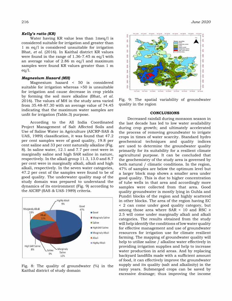
216 June 2020

Kelly’s ratio (KR) Water having KR value less than 1meq/l is

considered suitable for irrigation and greater than 1 m eq/l is considered unsuitable for irrigation Bhat, et al. (2016). In Kaithal district KR values were found in the range of 1.36-7.45 m eq/l with an average value of 2.86 m eq/l and maximum samples were found KR values greater than 1 m eq/l.

Magnesium Hazard (MH) Magnesium hazard < 50 is considered

suitable for irrigation whereas >50 is unsuitable for irrigation and cause decrease in crop yields by forming the soil more alkaline (Bhat, et al. 2016). The values of MH in the study area varied from 35.48-87.30 with an average value of 74.45 indicating that the maximum water samples are unfit for irrigation (Table.3) purpose.

According to the All India Coordinated Project Management of Salt Affected Soils and Use of Saline Water in Agriculture (AICRP-SAS & UAS, 1989) classification, it was found that 47.2 per cent samples were of good quality, 19.8 per cent saline and 33 per cent naturally alkaline (Fig. 8). In saline water, 12.1 and 7.7 per cent were in marginally saline and high SAR saline in nature, respectively. In the alkali group 11.3, 13.0 and 8.7 per cent were in marginally alkali, alkali and high alkali, respectively. In the seven water categories, 47.2 per cent of the samples were found to be of good quality. The underwater quality map of the study domain was prepared to understand the dynamics of its environment (Fig. 9) according to the AICRP (SAS & UAS-1989) criteria.

Fig. 8: The quality of groundwater (%) in the Kaithal district of study domain

Fig. 9: The spatial variability of groundwater quality in the region

CoNCLuSIoNSDecreased rainfall during monsoon season in

the last decade has led to low water availability during crop growth; and ultimately accelerated the process of removing groundwater to irrigate crops in times of water scarcity. Standard hydro geochemical techniques and quality indices are used to determine the groundwater quality primarily for its suitability for a resilient climate agricultural purpose. It can be concluded that the geochemistry of the study area is governed by both natural / climatic conditions. In the region, 47% of samples are below the optimum level but a larger block map shows a smaller area under good quality. This is due to higher concentration of tube wells in that area and accordingly more samples were collected from that area. Good quality groundwater is mostly lying in Guhla and Pundri blocks of the region and highly scattered in other blocks. The area of the region having EC < 2 can come under good quality category, but among those area where SAR < 10 and RSC ≥ 2.5 will come under marginally alkali and alkali categories. The results obtained from the study will help identify the conditions of low water quality for effective management and use of groundwater resources for irrigation use for climate resilient farming. The mapping of groundwater quality will help to utilize saline / alkaline water effectively in providing irrigation supplies and help to increase water production in arid areas. And by replacing backyard landfills made with a sufficient amount of food, it can effectively improve the groundwater supply and its quality (salt and alkalinity) in the rainy years. Submerged crops can be saved by excessive drainage; thus improving the income

of the farmer. Monsoonal rainfall, which plays a crucial role in the desalinization cycle, is also a factor regulating the seasonal salt balance in the root zone to permit saline-water use even with traditional irrigation methods for attaining of sustainable and resilient crop production.

reFereNCeSAdhikari, K., Chakraborty, B. and Gangopadhaya,

A. (2012). Assessment of irrigation potential of groundwater using water quality index tool. Environmental Research Journal. 6 (3) : 197-205.

AICRP - SAS & UAS. (1989). Annual Progress Report. All India Co-ordinated Research Project on Management of Salt-affected Soils and Use of Saline Water in Agriculture, CSSRI, Karnal, Haryana, India. https://aicrp.icar.gov.in/sasusw/about-us/

Anurag, Singh D and Surender Singh. (2009). Geographical Information Systems (GIS) Applications in Agrometeorology. Journal of Agrometeorology. 11 (Spl Issue) : 208-216.

Bhat, A. M., Grewal, M .S., Ramprakash, Rajpaul, Wani, A. S. and Dar, A E. (2016). Assessment of groundwater quality for irrigation purposes using chemical indices. Indian Journal of Ecology. 43 (2) : 574-579.

Cucci, G. Lacolla, G. and Rubino, P. (2013). Irrigation with saline-sodic water: Effects on soil chemical-physical properties. African Journal of Agricultural Research, 8 (4) : 358-365

Doneen, L. D. (1964). Water quality for agriculture. Department of Irrigation, University of California, Davis, USA.

Eaton, F .M. (1950). Significance of carbonates in irrigation waters. Soil Science., 69: 123–133.

Haritash, A.K., Kaushik, C.P., Kaushik, A., Kansal, A., and Yadav, A.K. (2008). Suitability assessment of groundwater for drinking, irrigation and industrial use in some North Indian villages. Environmental Monitoring and Assessment, 145 (1–3) : 397–406.

Kelley, W. P. (1940). Permissible composition and concentration of irrigation water. Proceedings of the American Society of Civil Engineers. 66: 607–613.

Mehta R. and Pandey V. (2015). Reference evapotranspiration (ETo) and crop water requirement (ETc) of wheat and maize in Gujarat. Journal of Agrometeorology 17 (1)

: 107-113.Raju, N.J., Shukla, U.K., & Ram, P. (2011).

Hydro-geochemistry for the assessment of groundwater quality in Varanasi: a fast-urbanizing center in Uttar Pradesh, India. Environmental Monitoring and Assessment, 173: 279–300.

Rathi, P. Ramprakash, Sharma, Raman and Rathi, N. (2018). Characterization of groundwater quality of Kalayat block of Kaithal district, Haryana. International Journal of Chemical Studies., 6 (1) :981-985.

Richards, L. A. (1954). Diagnosis and Improvement of Saline and Alkali Soils: U.S. Department of Agriculture Handbook., 60: Pp 160.

Singh, J. Shanwal, A. V. and Verma, S. L. (2000). Poor quality irrigation water and secondary salinization in semi-arid region of Rajasthan. Annals of Agri. Bio. Research., 5 (2) : 127-130.

Singh, K. P., Malik, A., Mohan, D, Vinod, K. S. and Sinha, S. (2006). Evaluation of Groundwater Quality in Northern Indo-Gangetic Alluvium Region. Environmental Monitoring and Assessment., 112: 211-230.

Singh Surender, Singh D, Sheokand R.N and Rao V.U.M. (2009). Web based Agrometeorological Information System for Sustainable Agricultural Development. Journal of Agrometeorology. 11 (Spl Issue) : 234-237.

Singh S., Brunini O. and Singh D. (2012). Real time Agrometeorological Information for contingent measures in attaining sustainable crop production. Journal of Agrometeorology. 14 (Spl Issue) :407-412.

Szabolcs A. and Darab, C. (1964). The influence of irrigation water of high sodium carbonate content of soils. In: Proceedings of 8th International Congress of ISSS, Transmission. 2 : 803–812.

Toumi, N. Hussein, B. H. M. Rafrafi, S. and Neama, E. (2015). Groundwater quality and hydro-chemical properties of Al-Ula Region, Saudi Arabia. Environmental Monitoring and Assessment. 187: 1-16.

Yadagiri, K. Sundaraiah, R. and Sateesh, P. (2015). Assessing Groundwater Quality and its Suitability for Irrigation purpose in Kothur area, Mahabubnagar District, Telangana State, India. Indian Journal of Applied Research. 5 (1) : 222-225.


Pre-harvest Yield Prediction of Mustard in Central Punjab using InfoCrop Model

KavIta Bhatt, K. K. gILL aNd MaMta raNa1

Communication Centre, Punjab Agricultural University, Ludhiana 141001, India1 CEEES, DCRUST S & T, Murthal, Sonipat, Haryana, India


aBStraCtThe pre-harvest prediction of mustard yield using Info Crop (V2.0) model in central Punjab was made for current years. The InfoCrop model was calibrated using six years data from 2000-01 to 2005-06 and validated with field data collected during 2006-07 to 2011-12 to obtain the probable mustard yield. The yield was predicted with the validated model for years 2012-13 to 2017-18. The prediction was done for three mustard cultivars i.e. cv. GSL1 sown on 25th October (D1), PBR91 sown on 15th November (D2) and cv. GSC6 sown on 5th December (D3). The average actual yield for the 5 years was 1363 kg/ha and the average predicted mustard yield for D1, D2 and D3 was 1333 kg/ha, 1400 kg/ha and 1374 kg/ha, respectively. The model explained 74% (GSL-1), 86% (PBR 91) and 93 % (GSC 6) variation in mustard yield when sown on different dates. The average per cent deviation during forecast period of 5 years for D1, D2 and D3 was -2.0, 3.0 and 1.0 % respectively which showed the importance of the study. InfoCrop model can be used for real time in-season mustard yield prediction.

Keywords: Mustard, Simulation model, InfoCrop, Yield, Sowing dates.

India is the second largest vegetable oil producer after China (Hedge, 2005, Boomiraj et al., 2010). Oleiferous Brassicas are important rabi (post-rainy) season oil seed crops in India and occupies a premier position due to its high oil content. Brassica is actually hyper sensitive to weather and show quiet distinct pattern of development and growth under different combinations of environmental conditions. Alam et al. (2015) reported that significant variations due to different planting dates were observed in plant height, number of leaves plant, weight plot, yield plot and yield of mustard. Lal et al. (2020) stated that the mustard production and productivity in the hot region of Rajasthan is dominated by both genetic makeup and environmental conditions. The temperature and solar radiation, amongst all weather parameters, are the most dominant factors affecting the crop growth, timing of occurrence of different phenological stages and crop yield under irrigated condition and they can be utilised for estimating and predicting the crop growth, crop phenology and production in advance. The rate of crop developmental stages is significantly affected by temperature such as leaf appearance rate is controlled mostly by temperature of leaf expansion zones (McMaster et al., 2003). Since, mustard is sensitive to climatic variables, the increased climatic variability under changing climate would create additional stress to crop growth during the season and have significant impact on its

production. It is anticipated that mean surface temperature of the earth is expected to be in the range of 0.3 to 0.7°C during the period 2016 to 2035 (IPCC, 2014). Crop yield production during cold season might become extra vulnerable due to higher uncertainties in rainfall and increase in temperature (Mall et al., 2004). The worldwide experiments projected 10 to 40% decline in different crop yield in India by 2080 to 2100 due to climate change (Vyankatrao, 2017, Rana, et al., 2018).

“The crop simulation models can be helpful for simulating the complex intercommunications across wide range of various factors viz, soil properties, weather and crop management, affecting crop performance (Shamim et al., 2012, Rana et al., 2018). The genetic coefficients of different mustard cultivars were derived as represented in Table 2. The purpose of the present study was to evaluate the effect of changes in climatic condition on mustard crop. Since the InfoCrop model was employed for such estimation, the objective of the present study was to calibrate and validate the model and predict mustard yield.

MaterIaLS aNd MethodSAgrometeorological data

Three Brassica cultivars, viz GSL 1, PBR 91 and GSC 6 were used to calibrate the model sown on different dates i.e. 25th October (D1),


15th November (D2) and 5th December (D3) for six years (2000-01 to 2005-06). The model was validated using the yield data of mustard for the period 2006-07 to 2011-12. The yield data was extracted from the statistical abstract of Punjab . The weather data for maximum temperature, minimum temperature, vapour pressure, bright sunshine hours, rainfall and wind speed was collected from agrometeorological observatory installed at PAU, Ludhiana to modify weather files and weather master modules in the model.

Crop simulation modelInfoCrop (V2.0) model is a crop simulation

model with sensitivity to crop cultivars, agronomic practices, soil, weather, flooding, frost and pests” (Aggarwal et al., 2006a and 2006b). This model considered the processes related to growth of crop, effect of waterloss, flood, nitrogen level management, frost and temperature stresses, crop and pest interactions, water soil and nitrogen balance and (soil) organic carbon dynamics. In the current study, the InfoCrop model was utilised to concoct the effects of soil, weather and crop management aspects on mustard yield.

Statistical analysisInfoCrop model performance was assessed

by analysing different statistical parameters viz. Coefficient of Determination (R2), Normalised Residual Mean Square Error (NRMSE), Mean Bias Error (MBE) and Per cent Deviation. The NRMSE describes about mean absolute deviation between observed and simulated and accuracy of simulation is characterized by lower” NRMSE. Mean bias error (MBE) represents over and under estimation of the predicted values. Percent deviation from observed values were also used to evaluate the accuracy of the model based mustard

prediction.

reSuLtS aNd dISCuSSIoN”Calibration of the model

The model was firstly calibrated adequately using the data for three Brassica cultivars, viz. GSL 1, PBR 91 and GSC 6 for three different dates of sowing i.e. 25th October, 15th November and 5th December for six years (2000-01 to 2005-06). The result indicated that the model was able to exaggerate fairly well for different treatments. Comparison of actual and forecast yield of different cultivars of mustard sown under different dates in the years 2001-2006 for Ludhiana was represented in Table 1. For the mustard cultivar GSL 1 sown on 25th October, per cent error ranged between -6.5 (2005-06) to 3.9 (2003-04), whereas, for cultivar PBR91 sown on 5th November, minimum per cent error was 1.4% during the year 2004-05 and maximum was 8.0 % recorded during the year 2003-04. When we compared the predicted yield to actual yield for cultivar GSC 6, per cent error ranged between -3.3 (2000-01) to 8.7 % (2001-02). Mote et al. (2016) reported that InfoCrop model was recently developed model and used in few crops of legume family like chickpea, cotton, mustard, soybean and groundnut.

Validation of the modelThe InfoCrop model was validated using

independent dataset for different cultivars sown on different dates during the year 2006-07 to 2011-12. The yields for different treatments, cultivars and years were simulated and compared with the observed yields. The results as given in Table 3 indicated least per cent error (-5.3) during the year 2009-10 for the cultivar GSL 1 and maximum of 7.8 % during the year 2006-07.

Table 1: Calibration of actual and forecasted yield of different cultivars of mustard sown under different dates from 2001-2006 for Ludhiana

Years actual Yield

Modeled Yield (kg/ha) 25th october

(gSL 1) 15th November

(PBr 91) 5th december

(gSC 6) Predicted

Yield% error Predicted


Yield% error

2000-01 1403 1453 3.6 1441 2.7 1357 -3.32001-02 1364 1397 2.4 1436 5.3 1482 8.72002-03 1197 1212 1.3 1281 7.0 1227 2.52003-04 1348 1400 3.9 1456 8.0 1402 4.02004-05 1577 1583 0.4 1599 1.4 1541 -2.32005-06 1359 1270 -6.5 1408 3.6 1396 2.7

Vol. 22, Special Issue BHATT et al. 219

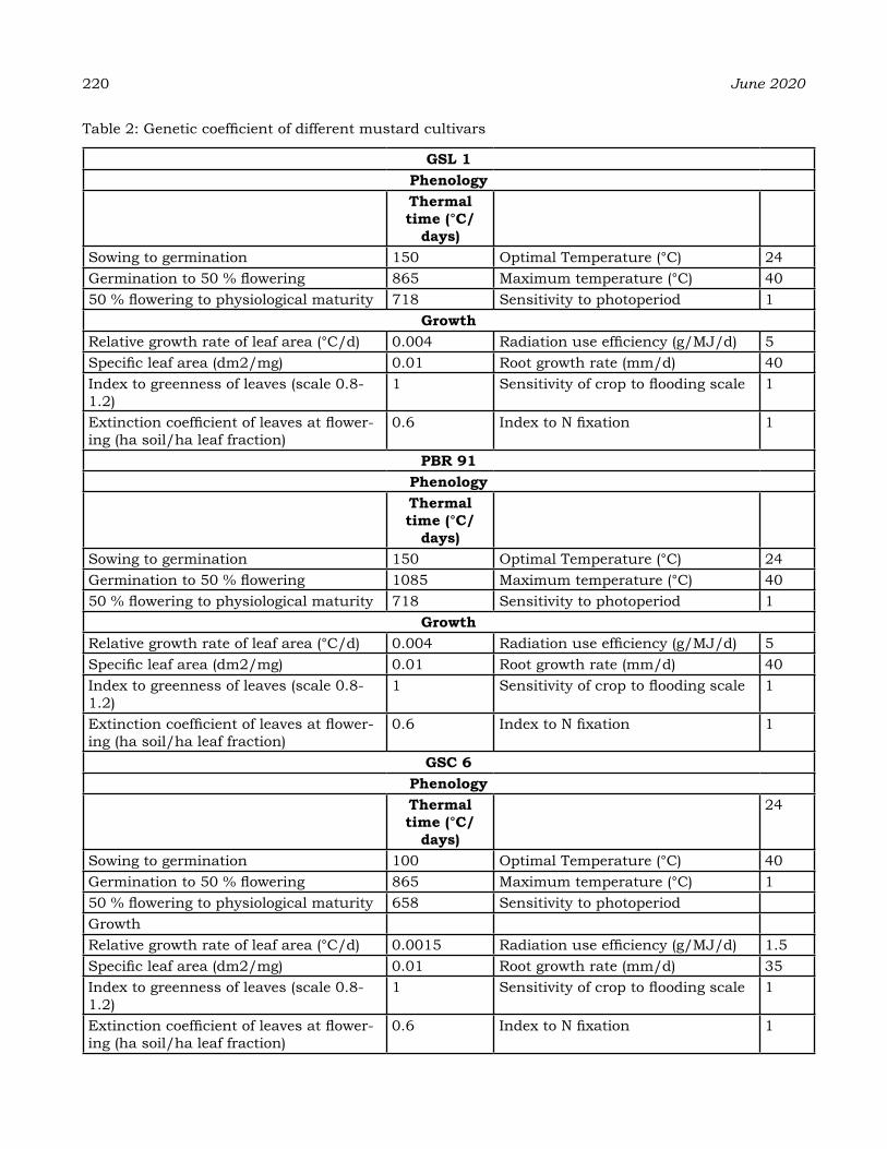
220 June 2020

Table 2: Genetic coefficient of different mustard cultivars

gSL 1Phenologythermal time (°C/

days) Sowing to germination 150 Optimal Temperature (°C) 24Germination to 50 % flowering 865 Maximum temperature (°C) 4050 % flowering to physiological maturity 718 Sensitivity to photoperiod 1

growthRelative growth rate of leaf area (°C/d) 0.004 Radiation use efficiency (g/MJ/d) 5Specific leaf area (dm2/mg) 0.01 Root growth rate (mm/d) 40Index to greenness of leaves (scale 0.8-1.2)

1 Sensitivity of crop to flooding scale 1

Extinction coefficient of leaves at flower-ing (ha soil/ha leaf fraction)

0.6 Index to N fixation 1

PBr 91Phenologythermal time (°C/

days) Sowing to germination 150 Optimal Temperature (°C) 24Germination to 50 % flowering 1085 Maximum temperature (°C) 4050 % flowering to physiological maturity 718 Sensitivity to photoperiod 1

growthRelative growth rate of leaf area (°C/d) 0.004 Radiation use efficiency (g/MJ/d) 5Specific leaf area (dm2/mg) 0.01 Root growth rate (mm/d) 40Index to greenness of leaves (scale 0.8-1.2)




gSC 6Phenologythermal time (°C/

days)

24

Sowing to germination 100 Optimal Temperature (°C) 40Germination to 50 % flowering 865 Maximum temperature (°C) 150 % flowering to physiological maturity 658 Sensitivity to photoperiodGrowthRelative growth rate of leaf area (°C/d) 0.0015 Radiation use efficiency (g/MJ/d) 1.5Specific leaf area (dm2/mg) 0.01 Root growth rate (mm/d) 35Index to greenness of leaves (scale 0.8-1.2)




For the cultivar PBR 91, per cent error ranged between -1.8 (2011-12) to 8.0 % (2008-09). The comparisons between the actual and forecasted yield for the cultivar GSC 6 indicated minimum per cent error of -3.3 during the year 2011-12 and maximum of 3.9 per cent during the year 2008-09. Adak et al. (2009) predicted the growth and yield of Brasica juncea under semi-arid environment of Delhi. The simulation results overestimated the seed yield for both sowings and the seasons with a RMSE value of 3.14 that indicated significant difference between observed and simulated yield.

Prediction of mustard yieldAfter calibration and validation of InfoCrop

model, mustard yield was predicted for five years i.e. 2013-2017. Actual and predicted mustard yield was compared for all three cultivars and results are given in Table 4 and also shown as Fig. 1, 2 and 3. Average actual yield for the years 2012-13 to 2016-17 was 1346 kg/ha, whereas, average predicted yield was calculated 1333, 1400 and 1374 for the mustard cultivar GSL 1, PBR 91 and

GSC 6, respectively sown on different dates. For the mustard cultivar GSL 1, per cent error ranged between -8.9 to 8.8 %. Per cent error calculated in the range of -3.9 to 10.0 and -3.4 to 5.7 % for the cultivars PBR 91 and GSC 6, respectively. Kumar et al. (2017) also showed in their study that model evaluated seed yield were within acceptable limit (<15%) for mustard crop.

Fig 1: Comparison of actual mustard yield with predicted yield (1: GSL 1), (2: PBR 91), 3: (GSC 6) during the years 2013 to 2017

Table 3: Validation of actual and forecasted yield of different cultivars of mustard sown under different dates from 2007-2012 for Ludhiana

Years actual Yield



(PBr 91) 5th december

(gSC 6) Predicted



Yield% error

2006-07 1199 1292 7.8 1249 4.2 1236 3.12007-08 1106 1161 5.0 1184 7.1 1121 1.42008-09 1306 1397 7.0 1410 8.0 1357 3.92009-10 1235 1169 -5.3 1307 5.8 1232 -0.22010-11 1395 1434 2.8 1376 -1.4 1361 -2.42011-12 1584 1591 0.4 1555 -1.8 1532 -3.3

Table 4: Prediction of actual and forecasted yield of different cultivars of mustard sown under different dates from 2013-2017 for Ludhiana

Years actual Yield



(PBr 91) 15th November

(gSC 6) Predicted



Yield% error

2012-13 1234 1342 8.8 1358 10.0 1304 5.72013-14 1289 1263 -2.0 1390 7.8 1283 -0.52014-15 1421 1336 -6.0 1395 -1.8 1372 -3.42015-16 1343 1224 -8.9 1390 3.5 1374 2.32016-17 1527 1499 -1.8 1467 -3.9 1538 0.7


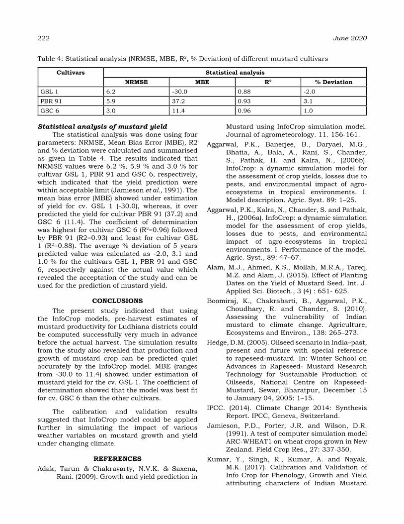
222 June 2020

Statistical analysis of mustard yieldThe statistical analysis was done using four

parameters: NRMSE, Mean Bias Error (MBE), R2 and % deviation were calculated and summarised as given in Table 4. The results indicated that NRMSE values were 6.2 %, 5.9 % and 3.0 % for cultivar GSL 1, PBR 91 and GSC 6, respectively, which indicated that the yield prediction were within acceptable limit (Jamieson et al., 1991). The mean bias error (MBE) showed under estimation of yield for cv. GSL 1 (-30.0), whereas, it over predicted the yield for cultivar PBR 91 (37.2) and GSC 6 (11.4). The coefficient of determination was highest for cultivar GSC 6 (R2=0.96) followed by PBR 91 (R2=0.93) and least for cultivar GSL 1 (R2=0.88). The average % deviation of 5 years predicted value was calculated as -2.0, 3.1 and 1.0 % for the cultivars GSL 1, PBR 91 and GSC 6, respectively against the actual value which revealed the acceptation of the study and can be used for the prediction of mustard yield.

CoNCLuSIoNSThe present study indicated that using

the InfoCrop models, pre-harvest estimates of mustard productivity for Ludhiana districts could be computed successfully very much in advance before the actual harvest. The simulation results from the study also revealed that production and growth of mustard crop can be predicted quiet accurately by the InfoCrop model. MBE (ranges from -30.0 to 11.4) showed under estimation of mustard yield for the cv. GSL 1. The coefficient of determination showed that the model was best fit for cv. GSC 6 than the other cultivars.

The calibration and validation results suggested that InfoCrop model could be applied further in simulating the impact of various weather variables on mustard growth and yield under changing climate.

reFereNCeSAdak, Tarun & Chakravarty, N.V.K. & Saxena,

Rani. (2009). Growth and yield prediction in

Mustard using InfoCrop simulation model. Journal of agrometeorology. 11. 156-161.

Aggarwal, P.K., Banerjee, B., Daryaei, M.G., Bhatia, A., Bala, A., Rani, S., Chander, S., Pathak, H. and Kalra, N., (2006b). InfoCrop: a dynamic simulation model for the assessment of crop yields, losses due to pests, and environmental impact of agro-ecosystems in tropical environments. I. Model description. Agric. Syst. 89: 1–25.

Aggarwal, P.K., Kalra, N., Chander, S. and Pathak, H., (2006a). InfoCrop: a dynamic simulation model for the assessment of crop yields, losses due to pests, and environmental impact of agro-ecosystems in tropical environments. I. Performance of the model. Agric. Syst., 89: 47–67.

Alam, M.J., Ahmed, K.S., Mollah, M.R.A., Tareq, M.Z. and Alam, J. (2015). Effect of Planting Dates on the Yield of Mustard Seed. Int. J. Applied Sci. Biotech., 3 (4) : 651- 625.

Boomiraj, K., Chakrabarti, B., Aggarwal, P.K., Choudhary, R. and Chander, S. (2010). Assessing the vulnerability of Indian mustard to climate change. Agriculture, Ecosystems and Environ., 138: 265–273.

Hedge, D.M. (2005). Oilseed scenario in India–past, present and future with special reference to rapeseed-mustard. In: Winter School on Advances in Rapeseed- Mustard Research Technology for Sustainable Production of Oilseeds, National Centre on Rapeseed-Mustard, Sewar, Bharatpur, December 15 to January 04, 2005: 1–15.

IPCC. (2014). Climate Change 2014: Synthesis Report. IPCC, Geneva, Switzerland.

Jamieson, P.D., Porter, J.R. and Wilson, D.R. (1991). A test of computer simulation model ARC-WHEAT1 on wheat crops grown in New Zealand. Field Crop Res., 27: 337-350.

Kumar, Y., Singh, R., Kumar, A. and Nayak, M.K. (2017). Calibration and Validation of Info Crop for Phenology, Growth and Yield attributing characters of Indian Mustard

Table 4: Statistical analysis (NRMSE, MBE, R2, % Deviation) of different mustard cultivars

Cultivars Statistical analysisNrMSe MBe R2 % deviation

GSL 1 6.2 -30.0 0.88 -2.0PBR 91 5.9 37.2 0.93 3.1GSC 6 3.0 11.4 0.96 1.0

Varieties in Semi- Arid Region of Haryana.Vegetos- An Int. J. Plant Res., 30 (4) : 1-5.

Kumar, Yogesh & Singh, Raj & Kumar, Anil & Chhabra, Karan & Nayak, Mukesh & Singh, Surender. (2018). Evaluation of InfoCrop model for simulating the performance of Indian-mustard varieties under different growing environment in western Haryana. Journal of Agrometeorology. 20. 188-192.

Lal, Manohar, Kumar, Sheilendra, Kumawat, S.M., Yadav, R.S. and Kharia, S.K. (2020). Performance of Mustard (Brassica juncea L.) varieties under Azadirachta indica L. shade and open condition in hot arid region of Rajasthan. Journal of Agrometeorology 22 (2) : 132-139.

Mall, R.K., Lal, M., Bhatia, V.S., Rathore, L.S. and Singh, R. (2004). Mitigating climate change impact on soybean productivity in India: a simulation study. Agric. Forest eteorol., 121:113-125.

Mote, B. M., Vasani, M. J., Ahir, H. K., Yadav, S. B. and Pandey V. (2016). Simulation of Phenology and Yield Attributing Characters of Legume Crops Using DSSAT and InfoCrop Model. Advances in Life Sciences 5 (13), Print: ISSN 2278-3849, 5265-5271.

McMaster, G.S. and Wilhelm, W.W. (2003). Phenological responses of wheat and barley to water and temperature: Improving simulation models. The Journal of Agricultural Sciences 141 (02) :129-147.

Rana, Mamta, Singh, K.K. and Kumari, Nisha (2018). Climate change assessment and projections in Haryana. Journal of Agrometeorology 20 (Special Issue) : 103-109.

Rana, Mamta, Singh, K.K. and Kumari, Nisha (2018). Validation of DSSAT-CERES model for rice and wheat crops with field and MODIS derived data in Haryana, India. Int. Agricultural Engineering Journal 27 (4) : 411-417.

Shamim, A., Shekh, A. M., Vyas Pandey, Patel, H. R. and Lunagaria, M. M. (2012). Simulating the phenology growth and yield of aromatic rice cultivars using CERES- Rice model under different environments. J. Agrometeorol., 14 (1) : 31-34.

Vyankatrao, N.P. (2017). Impact of climate change on agricultural production in India: Effect on rice productivity. Bioscience Discovery, 8 (4) : 897-914.


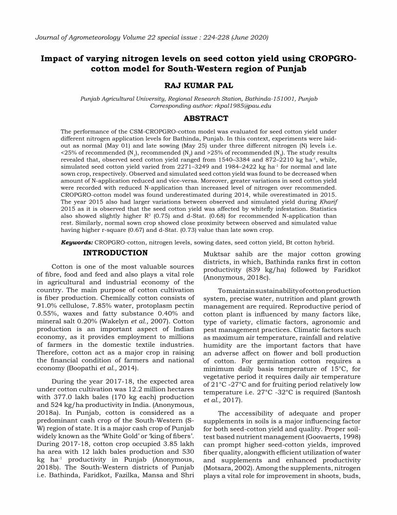
Impact of varying nitrogen levels on seed cotton yield using CroPgro-cotton model for South-Western region of Punjab

raJ KuMar PaLPunjab Agricultural University, Regional Research Station, Bathinda-151001, Punjab


aBStraCtThe performance of the CSM-CROPGRO-cotton model was evaluated for seed cotton yield under different nitrogen application levels for Bathinda, Punjab. In this context, experiments were laid-out as normal (May 01) and late sowing (May 25) under three different nitrogen (N) levels i.e. <25% of recommended (N1), recommended (N2) and >25% of recommended (N3). The study results revealed that, observed seed cotton yield ranged from 1540–3384 and 872–2210 kg ha-1, while, simulated seed cotton yield varied from 2271–3249 and 1984–2422 kg ha-1 for normal and late sown crop, respectively. Observed and simulated seed cotton yield was found to be decreased when amount of N-application reduced and vice-versa. Moreover, greater variations in seed cotton yield were recorded with reduced N-application than increased level of nitrogen over recommended. CROPGRO-cotton model was found underestimated during 2014, while overestimated in 2015. The year 2015 also had larger variations between observed and simulated yield during Kharif 2015 as it is observed that the seed cotton yield was affected by whitefly infestation. Statistics also showed slightly higher R2 (0.75) and d-Stat. (0.68) for recommended N-application than rest. Similarly, normal sown crop showed close proximity between observed and simulated value having higher r-square (0.67) and d-Stat. (0.73) value than late sown crop.

Keywords: CROPGRO-cotton, nitrogen levels, sowing dates, seed cotton yield, Bt cotton hybrid.

INtroduCtIoN

Cotton is one of the most valuable sources of fibre, food and feed and also plays a vital role in agricultural and industrial economy of the country. The main purpose of cotton cultivation is fiber production. Chemically cotton consists of 91.0% cellulose, 7.85% water, protoplasm pectin 0.55%, waxes and fatty substance 0.40% and mineral salt 0.20% (Wakelyn et al., 2007). Cotton production is an important aspect of Indian economy, as it provides employment to millions of farmers in the domestic textile industries. Therefore, cotton act as a major crop in raising the financial condition of farmers and national economy (Boopathi et al., 2014).

During the year 2017-18, the expected area under cotton cultivation was 12.2 million hectares with 377.0 lakh bales (170 kg each) production and 524 kg/ha productivity in India. (Anonymous, 2018a). In Punjab, cotton is considered as a predominant cash crop of the South-Western (S-W) region of state. It is a major cash crop of Punjab widely known as the ‘White Gold’ or ‘king of fibers’. During 2017-18, cotton crop occupied 3.85 lakh ha area with 12 lakh bales production and 530 kg ha-1 productivity in Punjab (Anonymous, 2018b). The South-Western districts of Punjab i.e. Bathinda, Faridkot, Fazilka, Mansa and Shri

Muktsar sahib are the major cotton growing districts, in which, Bathinda ranks first in cotton productivity (839 kg/ha) followed by Faridkot (Anonymous, 2018c).

To maintain sustainability of cotton production system, precise water, nutrition and plant growth management are required. Reproductive period of cotton plant is influenced by many factors like, type of variety, climatic factors, agronomic and pest management practices. Climatic factors such as maximum air temperature, rainfall and relative humidity are the important factors that have an adverse affect on flower and boll production of cotton. For germination cotton requires a minimum daily basis temperature of 15°C, for vegetative period it requires daily air temperature of 21°C -27°C and for fruiting period relatively low temperature i.e. 27°C -32°C is required (Santosh et al., 2017).

The accessibility of adequate and proper supplements in soils is a major influencing factor for both seed-cotton yield and quality. Proper soil-test based nutrient management (Goovaerts, 1998) can prompt higher seed-cotton yields, improved fiber quality, alongwith efficient utilization of water and supplements and enhanced productivity (Motsara, 2002). Among the supplements, nitrogen plays a vital role for improvement in shoots, buds,


leaves, roots, and bolls, while, phosphorus for early root advancement, photosynthesis and so forth.

The crop output mostly depends on the coordinated reactions of soil, climate and crop management practices that can be quantified utilizing a very much adjusted and validated crop models. CROPGRO-Cotton is comprehensively utilized as a technological tool for the tactical decision in order to have better harvest of cotton (Jones et al., 2003; Hoogenboom et al., 2010). Keeping in view the importance of nutrients on crop production, this study was carried out to assess the impact of varying nitrogen levels on seed cotton yield using CROPGRO-cotton model.

MaterIaLS aNd MethodSClimatic conditions of study location and experimental details:

The area of Bathinda lies in the outrageous South–West part of Punjab that falls in fourth Agro Climatic zone (ACZ). The climate of this area is semi-arid and normal yearly precipitation is 436 mm. The soil in the region is loamy sand to sandy loam in texture.

Dust storms are a regular feature in summer season when the mercury sometime touches over 47°C in the month of May-June, however, in winter during December and January & the minimum temperature at night could touch 0°C.

In order to quantify impact of varying nitrogen levels on seed cotton yield using CROPGRO-cotton model, field experiment was conducted at Punjab Agricultural University, Regional Station, Bathinda (30°58’N, 74°18’E) during Kharif season of 2014 and 2015. The crop was sown with two sowing environments as normal (D1=May 01) and late sown crop (D2=May 25) along with three nitrogen levels (N1 = <25% of Recommended, N2 = Recommended and N3 = >25% of Recommended).

Field experimental and CROPGRO-cotton model data:

The CROPGRO (Crop Growth) – Cotton model was used for simulation of seed cotton yield as affected by varying nitrogen levels. In view of that, field data were recorded from the research trials conducted in two consecutive years for the Bt cotton hybrid ‘NCS 855 BGII’. Using the model, comparative as well as statistical analysis of the data between actual and simulated seed cotton yield was done as treatment wise, year wise and

overall (output of the model with all the treatment and year, together). Weather parameters were recorded during study period from agro-meteorological observatory of the University (that is about 20 m away from the experimental site) (Fig. 1).

Fig. 1: Weekly weather conditions of temperature, humidity and rainfall during study periods of Kharif 2014 and 2015 at Bathinda

For the simulation of seed cotton yield at different sowing dates and varying nitrogen levels, already calibrated and validated genotypic coefficients for the Bt cotton hybrid ‘NCS 855 BGII’ have been used. These genetic coefficients were generated by Pal et al., (2016) with the help of GENCALC software (DSSAT) from the experimental data of 2011-12 to 2013-14.

The seed cotton yield was analyzed by standard deviation (SD) indicating the amount of variability of a set of values, and the low value indicates closer to the given mean and RMSE indicate how the clustered data is along the best fit axis. Model was also evaluated in terms of d-Statistics and R2 which allowed comparative evaluation of model performance at different locations while linear regression lines represented model stability via variable climatic conditions.

reSuLtS aNd dISCuSSIoNEvaluation of CROPGRO-cotton model in

terms of seed cotton yield as influenced by sowing environments and varying nitrogen levels:

Evaluation of the CROPGRO–Cotton model in terms of seed cotton yield based on different sowing dates and varying nitrogen levels using experimental data of Kharif 2014 and 2015 have been shown in Table 1 and illustrated in Fig. 2 and 3.

Vol. 22, Special Issue RAJ KUMAR PAL 225

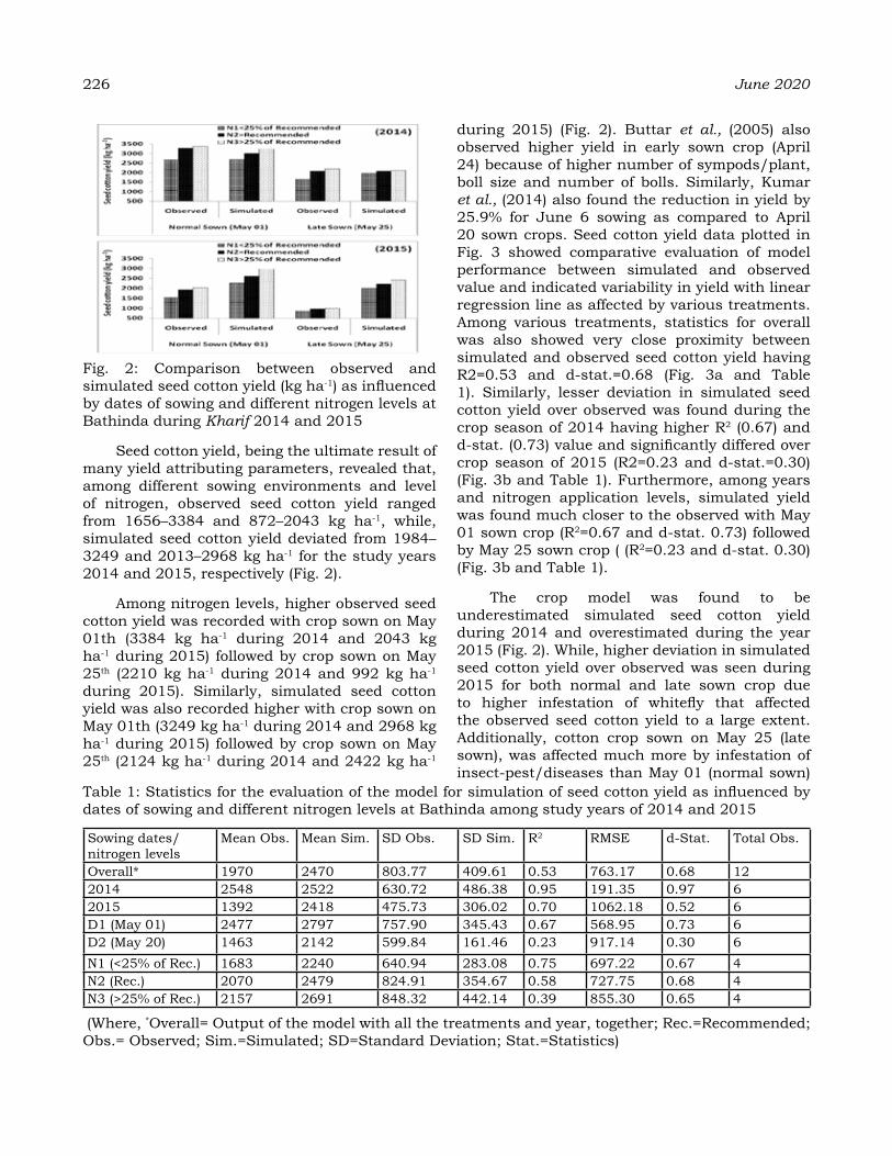
226 June 2020

Fig. 2: Comparison between observed and simulated seed cotton yield (kg ha-1) as influenced by dates of sowing and different nitrogen levels at Bathinda during Kharif 2014 and 2015

Seed cotton yield, being the ultimate result of many yield attributing parameters, revealed that, among different sowing environments and level of nitrogen, observed seed cotton yield ranged from 1656–3384 and 872–2043 kg ha-1, while, simulated seed cotton yield deviated from 1984–3249 and 2013–2968 kg ha-1 for the study years 2014 and 2015, respectively (Fig. 2).

Among nitrogen levels, higher observed seed cotton yield was recorded with crop sown on May 01th (3384 kg ha-1 during 2014 and 2043 kg ha-1 during 2015) followed by crop sown on May 25th (2210 kg ha-1 during 2014 and 992 kg ha-1 during 2015). Similarly, simulated seed cotton yield was also recorded higher with crop sown on May 01th (3249 kg ha-1 during 2014 and 2968 kg ha-1 during 2015) followed by crop sown on May 25th (2124 kg ha-1 during 2014 and 2422 kg ha-1

during 2015) (Fig. 2). Buttar et al., (2005) also observed higher yield in early sown crop (April 24) because of higher number of sympods/plant, boll size and number of bolls. Similarly, Kumar et al., (2014) also found the reduction in yield by 25.9% for June 6 sowing as compared to April 20 sown crops. Seed cotton yield data plotted in Fig. 3 showed comparative evaluation of model performance between simulated and observed value and indicated variability in yield with linear regression line as affected by various treatments. Among various treatments, statistics for overall was also showed very close proximity between simulated and observed seed cotton yield having R2=0.53 and d-stat.=0.68 (Fig. 3a and Table 1). Similarly, lesser deviation in simulated seed cotton yield over observed was found during the crop season of 2014 having higher R2 (0.67) and d-stat. (0.73) value and significantly differed over crop season of 2015 (R2=0.23 and d-stat.=0.30) (Fig. 3b and Table 1). Furthermore, among years and nitrogen application levels, simulated yield was found much closer to the observed with May 01 sown crop (R2=0.67 and d-stat. 0.73) followed by May 25 sown crop ( (R2=0.23 and d-stat. 0.30) (Fig. 3b and Table 1).

The crop model was found to be underestimated simulated seed cotton yield during 2014 and overestimated during the year 2015 (Fig. 2). While, higher deviation in simulated seed cotton yield over observed was seen during 2015 for both normal and late sown crop due to higher infestation of whitefly that affected the observed seed cotton yield to a large extent. Additionally, cotton crop sown on May 25 (late sown), was affected much more by infestation of insect-pest/diseases than May 01 (normal sown)

Table 1: Statistics for the evaluation of the model for simulation of seed cotton yield as influenced by dates of sowing and different nitrogen levels at Bathinda among study years of 2014 and 2015

Sowing dates/ nitrogen levels

Mean Obs. Mean Sim. SD Obs. SD Sim. R2 RMSE d-Stat. Total Obs.

Overall* 1970 2470 803.77 409.61 0.53 763.17 0.68 122014 2548 2522 630.72 486.38 0.95 191.35 0.97 62015 1392 2418 475.73 306.02 0.70 1062.18 0.52 6D1 (May 01) 2477 2797 757.90 345.43 0.67 568.95 0.73 6D2 (May 20) 1463 2142 599.84 161.46 0.23 917.14 0.30 6N1 (<25% of Rec.) 1683 2240 640.94 283.08 0.75 697.22 0.67 4N2 (Rec.) 2070 2479 824.91 354.67 0.58 727.75 0.68 4N3 (>25% of Rec.) 2157 2691 848.32 442.14 0.39 855.30 0.65 4

(Where, *Overall= Output of the model with all the treatments and year, together; Rec.=Recommended; Obs.= Observed; Sim.=Simulated; SD=Standard Deviation; Stat.=Statistics)

sown crop (Kataria et al., 2019).

Fig. 3: Performance evaluation of simulated seed cotton yield over observed as (a) overall, b) year wise, c) sowing date wise and d) nitrogen level wise

Moreover, observed seed cotton yield was found decreased when amount of N-application reduced and vice-versa. Similar results, the role of nitrogen in enhancing seed cotton yield was also reported by Entry et al., (1996) ; Milap et al., (1996) ; Parkash and Prasad, (2000) ; Kumbhar et al., (2008). Additionally, greater variations in seed cotton yield were recorded with reduced N-application than increased level of nitrogen application over recommended. Statistics in terms of varying nitrogen levels also showed that CROPGRO-cotton model is a good model to

simulate seed cotton yield with higher R2 (0.75) and d-Stat. (0.67) for Recommended N-application level (N2) than <25% of recommended (N1) (R

2=0.58 and d-stat. =0.67) and >25% of recommended (N3) (R2=0.39 and d-stat. =0.65) (Fig. 3d and Table 1). Similarly, lesser root mean square error (RMSE) was found with the crop sown on May 01 (RMSE=191.35) and recommended nitrogen application (RMSE=697.22) (Table 1).

Effect of weather conditions on seed cotton yield of Bt cotton hybrid:

During Kharif season of 2014, average weekly maximum temperature (Tmax) and minimum temperature (Tmin) varied from 27.1°C to 46 °C and 7.9°C to 29.6°C, respectively. However, relative humidity (RH) was recorded in the range between 49% to 94% and 10% to 62% for maximum RH (RHmax) and minimum RH (RHmin), respectively. Rainfall (288.0mm during Kharif 2014) being one of the most important weather parameters contributes a lot for development of the crop. Similarly, during 2015, Tmax, Tmin, RHmax and RHmin were observed in the range between 27.3 °C –43.7 °C, 11.2°C –27.3 °C, 60% –95% and 15% –74%, respectively. Moreover, a total of 399.6mm rainfall was received during the study period of Kharif 2015 (Fig. 1). Although, higher mean maximum and minimum temperature was observed during crop season of Kharif 2014, but due to higher mean maximum and minimum relative humidity during crop season and negligible rainfall during 33 to 37 SMW (1.0mm) in 2015, cotton crop was much more influenced by insect-pest infestation and finally affected the seed cotton yield. On the other hand, due to proper distribution of rainfall during 33 to 37 SMW having 4 rainy days (163.6.0 mm) in 2014, which is the most critical period of the crop during which flowering to boll opening exists, insect-pest infestation was found very less (Kataria et al., 2019) that supported better growth, resulting better yield (Fig. 1).

CoNCLuSIoNAmong years and nitrogen application

levels, lesser deviation in simulated seed cotton yield over observed was found with timely sown crop which was significantly differed over late sowing. Moreover, observed and simulated seed cotton yield was found decreased when amount of N-application reduced and vice-versa. Additionally, greater variations in seed cotton yield were recorded with reduced nitrogen

Vol. 22, Special Issue RAJ KUMAR PAL 227

228 June 2020

application than increased level of nitrogen application over recommended. Statistics also showed closer proximity between observed and simulated seed cotton yield and indicated higher R2 and d-Stat. value along with lower RMSE for Recommended N-application level (N2) than <25% of recommended (N1) and >25% of recommended (N3). Overall, based on the magnitude of difference between ground truth data and simulated value, the CROPGRO–cotton simulation model was found proficient to simulate the seed cotton yield influenced by different sowing environments and varying nitrogen application, which indicated the possibility of using model for further as a decision-supporting tool for cotton production in the region to obtain higher yield.

reFereNCeSAnonymous (2018a). All India coordinated

research project report on cotton (2017-18). Anonymous (2018b). Area, production and

productivity of cotton (State-wise), The Cotton Corporation of India Ltd. Available online at https://cotcorp.org.in/statistics.aspx? pageid=4#area1.

Anonymous (2018c). Package of Practices for kharif Crops. Pp 46-64. Punjab Agricultural University, Ludhiana

Boopathi, N.M., Sathish, S., Dachinamoorthy, P., Kavitha, P and Ravikesavan, R. (2014). Usefulness and Utilization of Indian Cotton Germplasm. In: World Cotton Germplasm Resource pp: 119-136.

Buttar G.S., Mahey R.K and Aggarwal. N. (2005). Effect of sowing time and quality of irrigation water on the growth and yield of American cotton (Gossypium hirsutum). J. Cotton Res. Dev. 19:216-217.

Entry, J.A., Mitchell, C.C and Backman, C.B. (1996). Influence of management practices on soil organic matter, microbial biomass and cotton yield in Alabama’s Old rotation. Biol. Fert. Soils. 23 (4) :353-358.

Goovaerts, P. (1998). Geo-statistical tools for characterizing the spatial variability of microbiological and physic-chemical soil properties. Biol. Fertil. Soil. 27:315-334.

Hoogenboom, G., Jones, J.W., Wilkens, R.W., Batcheloro, W.D., Hunt, L.A., Boot, K.J., Singh, U., Uryasev, O., Bowen, W.T., Gijsman, A.J., du-Toit, A., White, J.W and Tsuji, G.Y. (2010). Decision support system for Agro-technology Transfer v4.5 [CD- ROM] University of Hawaii.

Jones, J.W., Hoogenboom, G., Porter, C.H., Boot,

K.J., Batchelor, W.D., Hunts, L.A., Wilkens, P.W., Singh, U., Gijsman, A.J. and Ritchie, J.T. (2003). DSSAT cropping system model. Eur. J. Agron., 18:235–265.

Kataria, S.K., Pal, R.K., Kumar, V. and Singh, P. (2019). Population dynamics of whitefly, Bemisia tabaci (Gennadius), as influenced by weather conditions infesting Bt cotton hybrid, J. Agrometeorol., 21 (4) : 504-509.

Kumar, R., Bhattoo, M.S., Punia, S.S., Bhusal, N and Yadav, S. (2014). Performance of different Bt cotton (Gossypium hirsutum L.) hybrids under varying dates of sowing. J. Cotton Res. Dev. 28 (2) :263–264.

Kumbhar, A.M., Buriro U.A., Junejo S., Oad F.C., Jamro, G.H., Kumbhar, B.A and Kumbhar, S.A. (2008). Impact of different nitrogen levels on cotton growth, yield and N-uptake planted in legume rotation, Pakistan J. Bot. 40 (2) :767–778.

Milap, C., Brar B.S., Dhillon N.S and Gill M.P.S. (1996). Response of cotton to applied K at different N levels in a cotton-wheat cropping system on a Typic Ustochrept in Punjab. J. Potassium Res. 12 (4) :370–375.

Motsara, M.R. (2002). Available nitrogen, phosphorus and potassium status of Indian soils as depicted by soil fertility maps. Fert. News 47 (8) :15-21.

Pal, R.K. (2018). Effect of temperature on various phenophases of cotton for South-Western region of Punjab, Progressive Research: An International Journal, 13 (Special Issue) :253-256.

Prakash, R and Prasad M. (2000). Effect of nitrogen, chlormequat chloride and farmyard manure applied to cotton (Gossypium hirsutum) and their residual effect on succeeding wheat (Triticum aestivum) crop. Indian J. Agron. 45 (2) :263-268.

Santosh, D.T., Tiwari, K.N., Singh, V.K and Reddy, A.R.G. (2017). Micro Climate Control in Greenhouse. Int. J. Curr. Microbiol. App. Sci. 6 (3) :1730-42.

Wakelyn, P.J., Bertoniere, N.R., French, A.D., Thibodeaux, D.P., Triplett, B.A., Rousselle, A.A., Goynes, W.R.J., Edwards, J.V., Hunter, L., Mcalister, D.D and Gamble, G.R. (2007). Cotton fiber chemistry and technology. CRC Press Boca Raton pp: 23–68.

Yadav, B.K., Sidhu, A.S and Kumar, D. (2018). Status of DTPA extractable micronutrients in soils of Bathinda district of Punjab, India, Agric. Res. J. 55 (2) :358-361.

evaluation of real time weather related fluctuations and wheat productivity in northern India

K.K.gILL, SatINder Kaur, S.S.SaNdhu aNd S.S.KuKaLCommunication Centre, PAU, Ludhiana-141004

Department of Climate Change & Agricultual Meteorology, PAU, LudhianaCorresponding Author Email: [email protected]

aBStraCtThe weather fluctuations are being felt globally in the form of changes in temperature and rainfall pattern. The increased concentration of green house gases (GHGs) viz. CO2, methane and nitrous oxides are resulting in the warming of climate systems by 0.74oC. Overall the temperature during winter season is likely to be much higher as compared to summer season. The minimum temperature during anthesis stage of wheat is considered to be the most important factor for wheat productivity and it remained between 11.7 to 12.4oC during lowest yield years. The maximum temperature during anthesis and soft dough stage are also very critical. During high yield years the deviation of maximum temperature from normal was -0.1, -0.1 and -2.5ºC for 2011-12, 2013-14 and 2016-17, respectively. The warming is more pronounced over northwest India, agriculturally most important region of the country. The substantial changes in the environment are affecting Indian agriculture but not uniform across the country. The well-known General Circulation Models projected the climatic changes which will grossly impact the food-cropping system in years to come (Agarwal and Sinha, 2019).

Keywords: Weather parameters, wheat, temperature, rainfall, yield

INtroduCtIoN

In India, Agriculture and its allied sectors are the largest source of livelihoods. About 70 percent of its rural households still depend primarily on agriculture for their livelihood, with 82 percent of farmers being small and marginal (FAO, 2018). Keeping in mind the frequent weather fluctuations in terms of temperature and rainfall distribution in Punjab state observed in the recent years, it is important to study the impact of these weather fluctuations on crop productivity. Recently, Kaur et al., (2013) observed a significant increase in annual, winter (rabi) season and summer (kharif) season minimum temperatures across the agro-climatic zones of Punjab. In northern India, an increase of 2oC in mean temperature may reduce potential wheat yields (Aggarwal and Sinha, 1993). You et al., (2009) reported that increase in wheat growing season temperature by 1.8oC reduces wheat yields by about 3–10%. As the maximum temperature increases during the mid-anthesis period (76–79 DAS) the number of grains per ear at maturity declined. It has been shown that with increase in maximum temperature at 78 DAS the grain yield and harvest index also declined sharply (Ferris et al., 1998).

However, most of the studies related to

climate related effects on crop production are simulation studies. The actual impact of changing temperature conditions on wheat production is clearly reflected from the fact that wheat production in Punjab in northwest India during 2016-17 was exceptionally high (17636 thousand metric tonnes) due to abnormally good weather conditions (maximum temperature during soft dough stage remained 25.3ºC which was below normal by 2.5ºC). However, during 2014-15 wheat season, the production declined to 15050 thousand metric tonnes due to unfavourable weather conditions (minimum temperature during anthesis stage remained 11ºC and 12ºC, which was more than the normal by 2 and 3ºC) which prevailed at the far end of the maturity stage. The present study thus aims at analysing the weather-related fluctuations in wheat productivity over eight seasons (2009-17) with variable weather conditions in India Punjab.

MaterIaLS aNd MethodSStudy site

The study was conducted in north-western region of India, commonly known as food bowl of the country. The Punjab state has three distinct agro-climatic regions, viz. submontane region, central plains and south-western plains. Punjab


230 June 2020

is situated between 29.30° - 32.32° N latitudes and 73.55° - 76.50° E longitudes at an average altitude of 212 m above mean sea level.

Climate The climate of the region is determined by

the extreme hot and extreme cold conditions and comprises of different seasons. Among the three main seasons, the summer months includes span for two and half months i.e. mid April to the end of June. The monsoon season starts from early July and continues till September. The winter season is of mainly three months i.e. from early December to the end of February. The post-monsoon season and the post-winter season are the transitional seasons in the region. In Punjab, although the summer season commences from mid April but the mean temperature starts rising from February onwards. Afterwards, summers are followed by the rainy season. The rains are brought by the monsoonal winds blowing over the Bay of Bengal and Arabian Sea. During winters and the post-winter transitional season, very frequent hail storms and intermittent showers occur resulted in causing crop damage. The winds become dry by end of the March. The climate of Punjab has been playing a great role in uplifting the economy of the state.

Submontane Region: The mean maximum temperature in sub mountain undulating region normally ranges between 19.4 to 38.4 oC during the year, where the highest (38.4oC) and lowest maximum (19.4oC) is recorded during the month of May and January, respectively. The lowest (5.2oC) and highest (25.0oC) minimum is recorded during the month of January and July, respectively. The annual normal rainfall in the region is 1069.0 mm, maximum and minimum rainfall of 303.3 and 7.4 mm has been recorded during the month of August and November, respectively.

Central Plains: In central plains, the mean maximum temperature varies from 18.3 to 38.6oC and means minimum varies from 5.6 to 26.1oC. The highest maximum (38.6oC) and highest minimum (26.1oC) was recorded during the month of May and July, respectively. The lowest maximum and minimum are obtained during the month of January. The mean annual rainfall recorded in the region is 753.5 mm, maximum and minimum rainfall of 222.5 and 7.1 mm was recorded during the month of July and November, respectively.

Southwest Plains: In Southwest Plains region, normally the mean highest maximum temperature (40.4oC) occurs in the month of May while mean highest minimum (26.9oC) occurs during the month of July. The lowest minimum (4.8oC) and maximum (19.5oC) temperature was recorded, both during the months of January. The annual normal rainfall in the region is 529.0 mm. The highest and lowest normal rainfall of 135.6 and 4.6 mm occurs during the month of July and November, respectively

Data collectionThe data pertaining to weather parameters

viz. winter season maximum and minimum temperatures and rainfall during the wheat growing season (2009-17) were collected from the weather observatories located in the districts of Nawanshahar (Submontane Punjab), Ludhiana (Central Plains) and Bathinda (Southwest Plains) districts.

The data was analysed during the wheat season starting from sowing (30th October to 10th November) till harvesting of wheat crop (15th to 30th April) with respect to different wheat phenological stages During the study period, the sowing date was considered from 1st November to 3rd April for all the eight consecutive years (2009-17).The different phonological stages were sowing (0 DAS), to start emergence (5 DAS), complete emergence (8 DAS), crown root initiation (CRI) stage (24 DAS), tillering (31 DAS), jointing (49 DAS), booting (79 DAS), heading (94 DAS), anthesis (111 DAS), milking (126 DAS), soft dough (131 DAS), hard dough (143 DAS) and physiological maturity (148 DAS).

reSuLtS aNd dISCuSSIoNMinimum temperature: Minimum

temperature trend was analysed for central region during wheat season (109-123 DAS) from 2009-10 to 2016-17 (Fig. 1.a). The minimum temperature during anthesis stage is considered to be the most important factor for wheat productivity.

During the study period (2009-2017), the minimum temperature varied from 5.8-17.8 oC. During the lowest yield years, the minimum temperature during anthesis remained 11.7 and 12.4 ºC for 2009-10 and 2014-15, respectively. During these years the minimum temperature was more than normal by 2.9 ºC and 3.6 ºC in wheat season. During the highest yield years, there was increase in the minimum temperature

from the normal by 0.1, 0.3 and 1ºC, respectively during anthesis stage. The favourable minimum temperature during anthesis was found to be 8.9-9.8 ºC in whole season.

Fig. 1: (a-c) Minimum temperature trends at central, southwest and Sub mountain during wheat season 109-123 DAS

Similar trend was studied in south-west region, where the minimum temperature during the season (109-123 DAS) varied from 4.6 -15.6oC during the years 2009-10 to 2016. Higher the temperature during anthesis has negative effect on yield of the crop. Even a single day heat stress causes a significant decrease in individual grain mass and number (Talukder et al., 2013). The minimum temperature during lowest yield years during anthesis stage remained 11 ºC and 12 ºC for 2009-10 and 2014-15, respectively. During these years minimum temperature was more than the

normal by 2 and 3 ºC. The minimum temperature clearly indicates harsh and unfavourable weather conditions during 2009-10 and 2014-15 in all the regions for most of the season in all the agro-climatic regions of the state.

During highest yield years, the minimum temperature during anthesis remained 7.5, 8.3 and 9 ºC for 2011-12, 2013-14 and 2016-17, respectively. During these years minimum temperature was above the normal by -1.5, -0.7 and 0.0 ºC, respectively. The favourable minimum temperature during anthesis was found to be 7.5-9.0 ºC in whole season.

Similar trend was found in sub mountain undulating region, during lowest yield years, the minimum temperature during anthesis remained 10.9 and 11.2 ºC, which was above than normal by 1.7 and 2 ºC for 2009-10 and 2014-15, respectively. During high yield years, minimum temperature during anthesis remained 7.9, 9.2 and 9.9 ºC for 2011-12, 2013-14 and 2016-17and deviation of minimum temperature from the normal by -1.3, 0.0 and 0.7 ºC, respectively. The favourable minimum temperature during anthesis was found to be 7.9-9.9 ºC in whole season. Days taken for anthesis and maturity were reduced with increased in temperature. Prasad et al., (2018).

Maximum temperature: Maximum temperature trend was studied for central region during wheat season (111-142 DAS) (Fig. 2.a). During lowest yield year (2009-10), the maximum temperature during anthesis and soft dough remained 25.6 and 31.1 ºC. During 2009-10 maximum temperature at anthesis and soft dough stage was more than the normal by 3.0 and 4.7 ºC, respectively. During 2014-15 (low yield year) variation in maximum temperature was not found, but heavy rainfall was received for all three regions of northwest India.

During highest yield years, maximum temperature during anthesis stage remained 22.5 and 21.7 ºC, during soft dough stage 27.1 and 26.3 ºC for 2011-12 and 2013-14. During highest yield years (2011-12 and 2013-14), deviation in maximum temperature during anthesis stage was -0.1 and -0.8 ºC and during soft dough stage was 1.2 and -0.1 ºC, respectively. The favourable maximum temperature range during anthesis and soft dough stage was found to be 21.7-22.5 ºC and 26.1-27.1 ºC, respectively.

In south-western region, during low yield

Vol. 22, Special Issue GILL et al. 231

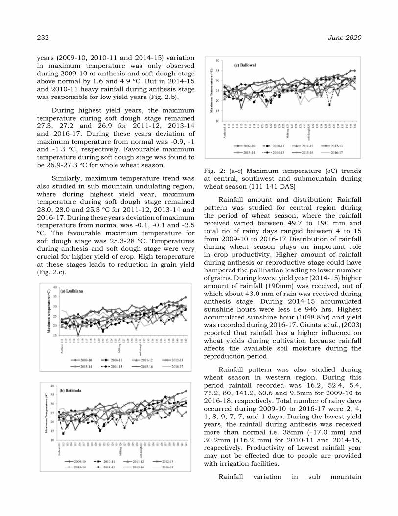
232 June 2020

years (2009-10, 2010-11 and 2014-15) variation in maximum temperature was only observed during 2009-10 at anthesis and soft dough stage above normal by 1.6 and 4.9 ºC. But in 2014-15 and 2010-11 heavy rainfall during anthesis stage was responsible for low yield years (Fig. 2.b).

During highest yield years, the maximum temperature during soft dough stage remained 27.3, 27.2 and 26.9 for 2011-12, 2013-14 and 2016-17. During these years deviation of maximum temperature from normal was -0.9, -1 and -1.3 ºC, respectively. Favourable maximum temperature during soft dough stage was found to be 26.9-27.3 ºC for whole wheat season.

Similarly, maximum temperature trend was also studied in sub mountain undulating region, where during highest yield year, maximum temperature during soft dough stage remained 28.0, 28.0 and 25.3 ºC for 2011-12, 2013-14 and 2016-17. During these years deviation of maximum temperature from normal was -0.1, -0.1 and -2.5 ºC. The favourable maximum temperature for soft dough stage was 25.3-28 ºC. Temperatures during anthesis and soft dough stage were very crucial for higher yield of crop. High temperature at these stages leads to reduction in grain yield (Fig. 2.c).

Fig. 2: (a-c) Maximum temperature (oC) trends at central, southwest and submountain during wheat season (111-141 DAS)

Rainfall amount and distribution: Rainfall pattern was studied for central region during the period of wheat season, where the rainfall received varied between 49.7 to 190 mm and total no of rainy days ranged between 4 to 15 from 2009-10 to 2016-17 Distribution of rainfall during wheat season plays an important role in crop productivity. Higher amount of rainfall during anthesis or reproductive stage could have hampered the pollination leading to lower number of grains. During lowest yield year (2014-15) higher amount of rainfall (190mm) was received, out of which about 43.0 mm of rain was received during anthesis stage. During 2014-15 accumulated sunshine hours were less i.e 946 hrs. Highest accumulated sunshine hour (1048.8hr) and yield was recorded during 2016-17. Giunta et al., (2003) reported that rainfall has a higher influence on wheat yields during cultivation because rainfall affects the available soil moisture during the reproduction period.

Rainfall pattern was also studied during wheat season in western region. During this period rainfall recorded was 16.2, 52.4, 5.4, 75.2, 80, 141.2, 60.6 and 9.5mm for 2009-10 to 2016-18, respectively. Total number of rainy days occurred during 2009-10 to 2016-17 were 2, 4, 1, 8, 9, 7, 7, and 1 days. During the lowest yield years, the rainfall during anthesis was received more than normal i.e. 38mm (+17.0 mm) and 30.2mm (+16.2 mm) for 2010-11 and 2014-15, respectively. Productivity of Lowest rainfall year may not be effected due to people are provided with irrigation facilities.

Rainfall variation in sub mountain

undulating region during the study year (2009-17) was observed. Amount of rainfall received during this period was 43.2, 191.5, 95.4, 163.6, 194.9, 292.3, 81.5 and 172.7 mm for 2009-10 to 2016-17. Highest amount of rainfall was received during low yield years (2010-11 and 2014-15). During 2010-11 highest amount of rainfall was received during jointing (74mm) and heading (93.5mm), which was higher than the normal by 38mm and 67.5mm. whereas, during 2014-15 higher amount of rainfall was recorded during anthesis (123.7mm) and soft dough (52mm) stage, which was more than the normal by 107.2mm and 38.7mm.

Wheat productivity: The wheat productivity during the study years (2009-17) was quite variable. On the basis of weather fluctuation observed during the study period, the years have been identified as low yield year, medium yield year and high yield year. Among the eight years lowest and highest yield was achieved during 2014-15 and 2016-17, respectively (Table 1). Grain yield decreased by 33.1% and straw yield increased by 10.8% with an increase in temperature by 3°C and an increase in solar radiation (up to 3MJ m-2 day-1) in comparison with the normal conditions (Prasad et al., 2018). The wheat productivity in submontane region was ranged from 3.7 (2014-15) to 4.9 t/ha (2013-14 and 2016-17), whereas corresponding grain yields in central Punjab and southwest Punjab varied from 4.4 (2014-15) to 5.4 t/ha (2011-12) and 4.6 (2009-10 and 2010-11) to 5.3 t/ ha (2016-17), respectively. The yields were lowest during 2009-10, 2014-15 and 2010-11 in all the regions. Among all the eight years under study, three years namely 2011-12, 2013-

14 and 2016-17 were highest crop yield years and two years namely, 2012-13 and 2015-16 were medium yield years. These fluctuations in wheat productivity during the eight-year period occurred despite of the crop cultivars of similar yield potential and similar agronomic management practices being followed during these years. The differential yield over a period of eight years thus seems to be related to differential weather conditions prevailing during these years.

Table 1: Yield (t/ha) of wheat crop of different years in three agro-climatic regions of Punjab

Year Submontane Punjab

Central Plains

Southwest Plains

2009-10 4.5 4.6 4.62010-11 4.3 5.0 4.62011-12 4.8 5.4 5.02012-13 4.8 4.8 4.72013-14 4.9 5.2 4.92014-15 3.7 4.4 4.82015-16 4.7 4.7 4.72016-17 4.9 5.1 5.3

CoNCLuSIoNSWeather during 2011-12, 2013-14 and 2015-

16 remained favourable for the crop but was not much favourable during 2009-10 and 2014-15.

During low yield years (2009-10 and 2014-15) average minimum temperature during anthesis stage was higher by 2.9 ºC and 3.6 ºC in central Punjab, 2 ºC and 3 ºC in south-western Punjab and by 1.7 ºC and 2 ºC in sub mountain

Table 2: Rainfall amount (mm) and number of rainy days during wheat season of different years in three agro-climatic regions of Punjab

Year

Sub mountain region Central region Southwest regionSunshine

hours (hrs)

Rain amount (mm)

rainy days (#)

Sunshine hours (hrs)

Rain amount (mm)

rainy days (#)

Rain amount (mm)

rainy days (#)

2009-10 852.9 43.2 5 1035.8 49.7 4 16.2 22010-11 905 191.5 9 943.9 74.2 7 52.4 42011-12 927.9 95.4 8 917.7 65.6 6 5.4 12012-13 955.7 163.6 16 1008.2 157.6 14 75.2 82013-14 912.8 194.9 18 971.8 145 14 80 92014-15 835.2 292.3 18 946 190 15 141.2 72015-16 851.9 81.5 9 949.3 71 8 60.6 72016-17 939.7 172.7 10 1048.8 94.1 6 9.5 1

Vol. 22, Special Issue GILL et al. 233

234 June 2020

undulating region on the other hand maximum temperature during soft dough stage in year 2009-10 remained higher than normal by 4.7, 4.9 and 3.7 ºC at these locations, respectively. Which might have adversely affected the productivity. Higher amount of rainfall at anthesis stage during 2014-15 (higher by 26mm at Bathinda and by 107.2mm at Ballowal than normal) might have reduced the productivity.

reFereNCeSAgarwal, N. and Sinha, A. (2019). Future climate

analogues of current wheat production zones in India. Current Sci., 116 (2) : 264-71.

Aggarwal, P.K. and Sinha, S.K. (1993). Effect of probable increase in CO2 and temperature on productivity of wheat in India. J. Agrometeorol., 48. 811-814.

Ferris, R., Ellis, R. H., Wheeler, T. R. and Hadley, P. (1998). Effect of High Temperature Stress at Anthesis on Grain Yield and Biomass of Field-grown Crops of Wheat. Ann. Bot., 82: 631–639.

Giunta, F., Motzo, R., and Deidda, M. (2003). Effect of drought on yield and yield components of durum wheat and triticale in a Mediterranean environment. Field Crops

Res., 33: 399- 409.Kaur Prabhjyot and Hundal, S. S. (2006). Effect of

Possible futuristic climate change scenarios on productivity of some kharif and rabi crops in the central agroclimatic zone of Punjab. J. Agril. Physics., 6: 21-27.

Kaur Prabhjyot, Sandhu, S.S., Singh, S. and Gill, K.K. (2013). Climate Change-Punjab Scenario. Bulletin:AICRPAM, School of Climate Change and Agricultural Meteorology, PAU, Ludhiana. pp16.

Prasad, G., Singh, S. M., Patel, C., Nema, A. K., Singh, R. S., Yadav, M. K. and Singh, K. K. (2018). Impact of temperature and solar radiation on wheat crop for Varanasi region of Uttar Pradesh. Vayu Mandal., 44: 47-52.

Talukder, A.S.M.H.M., McDonald, G. K., and Gill, G. S. (2013). Effect of short-term heat stress prior to flowering and at early grain set on the utilization of water-soluble carbohydrate by wheat genotype. Field Crops Res., 147: 1–11.

You, L., Rosegrant, M. W., Wood, S., and Sun, D. (2009) Impact of growing season temperature on wheat productivity in China. Agril. Forest Meteorol., 149: 1009–14.

annual trends of temperature and rainfall extremes in haryana for the period 1985-2014, INdIa

MaMta, raJ SINgh, SureNder SINgh, dIWaN SINgh, aNIL KuMar, dIveSh, aBhILaSh aNd aMIt Dept of Agricultural Meteorology

CCS Haryana Agricultural University, Hisar -125004 (India) Corresponding author Email id: [email protected]

aBStraCtLong-term meteorological data of 30 year period (1985-2014) for five locations viz. Ambala, Bawal, Hisar, Karnal and Sirsa, in both the Agro-climatic Zonesviz. Eastern and Western Zone (Planning Commission, 1989) in Haryana state were analyzed. Calculations were performed using the Excel template MAKESENS (Mann-Kendall test for trend and Sen’s slope estimator). The annual trend and slope values of temperature related climate change indicators for five locations in the state of Haryana indicated a decrease in the cold extreme event. The hot extreme events showed an increasing order. The trend and slope of night extremes (TR20 and TN90) were more potent than those in day extremes (TNn, TXn, ) resulting in the decrease of day-night temperature variation as demonstrated by constructing diurnal temperature range (DTR) for Bawal, Hisar, Karnal and Sirsa.Overall, the results showed widespread significant changes in temperature trends consistent with warming, especially for those indices derived from daily minimum temperature. Annual average trend for DTR in the state was -0.78 °C. The trend of rainfall indices in Haryana showed an increase in rainfall intensity for Bawal however the trends of rainfall indices showed no definite trends over different stations.

Keywords: RClimdex, temperature, Haryana, climate change indices, Mann-Kendall test & Sen’s slope

INtroduCtIoN

India is among the countries that are most vulnerable to climate change due to its high dependency on rain-fed agriculture and lack of adaptation strategies. Climate change impacts the natural ecosystems and is expected to have substantial adverse effects in India, mainly on agriculture on which 58 per cent of the population still depends for livelihood (Anonymous, 2017). Climate change will also cause increased frequency of extreme events such as floods and droughts The global mean surface temperature has shown warming of 0.89°C over the period 1901–2012 which is mainly attributed to anthropogenic activities and each of the last three decades has been warmer than all preceding decades since 1850 and the first decade of the 21st century has been the warmest (IPCC, 2013). Though the monsoon rainfall of the last few decades have no significant trend on an all India scale (Parthasarthy, 1984; Pant and Kumar, 1997), there are regional trends in the monsoons that have been observed in the past century (Rupa Kumar et al., 1994, Guhathakurta and Rajeevan, 2008, Krishna Kumar et al., 2010). Climatological variability and trends over the Koshi river basin were studied using RClimDex

by Shrestha et al. (2016).Results show that the frequency and intensity of weather extremes are increasing. The daily maximum temperature (TXx) increased by 0.1°C decade−1 on average between 1975 and 2010 and the minimum (TNn) by 0.3°C decade−1over Koshi river basin in India. However, there are certain regional differences in the annual & monsoon rainfall variability, which are of important consequences. Since, annual rainfall fluctuations under climate change scenarios are of vital importance to agriculture, water supply and energy planning, therefore, an attempt has been made to understand the rainfall behaviour in Haryana state to identify the optimal cropping strategies that ensure the sustainable ecological development under looming threats of climate change and variability. Intergovernmental Panel on Climate Change (IPCC) promulgated a clear message that there had been many extreme weather and climate events observed globally since 1950, and these changes occurred mainly due to anthropogenic causes and emission of greenhouse gases. A study was carried out to assess the extreme temperature and rainfall events for the period 1985–2014 at the five locations of Haryana by using ETCCDI indices through RClimDex software. The statistical significance


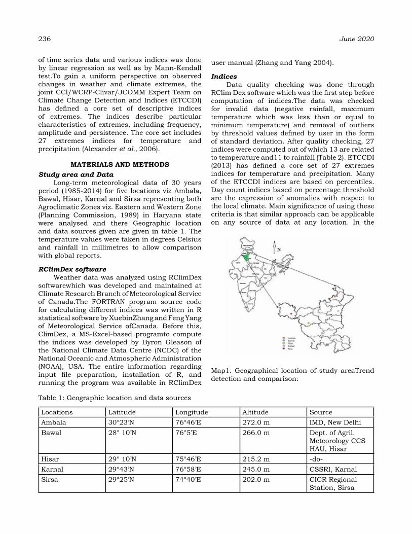
236 June 2020

of time series data and various indices was done by linear regression as well as by Mann-Kendall test.To gain a uniform perspective on observed changes in weather and climate extremes, the joint CCl/WCRP-Clivar/JCOMM Expert Team on Climate Change Detection and Indices (ETCCDI) has defined a core set of descriptive indices of extremes. The indices describe particular characteristics of extremes, including frequency, amplitude and persistence. The core set includes 27 extremes indices for temperature and precipitation (Alexander et al., 2006).

MaterIaLS aNd MethodSStudy area and Data

Long-term meteorological data of 30 years period (1985-2014) for five locations viz Ambala, Bawal, Hisar, Karnal and Sirsa representing both Agroclimatic Zones viz. Eastern and Western Zone (Planning Commission, 1989) in Haryana state were analysed and there Geographic location and data sources given are given in table 1. The temperature values were taken in degrees Celsius and rainfall in millimetres to allow comparison with global reports.

RClimDex softwareWeather data was analyzed using RClimDex

softwarewhich was developed and maintained at Climate Research Branch of Meteorological Service of Canada.The FORTRAN program source code for calculating different indices was written in R statistical software by XuebinZhang and Feng Yang of Meteorological Service ofCanada. Before this, ClimDex, a MS-Excel-based programto compute the indices was developed by Byron Gleason of the National Climate Data Centre (NCDC) of the National Oceanic and Atmospheric Administration (NOAA), USA. The entire information regarding input file preparation, installation of R, and running the program was available in RClimDex

user manual (Zhang and Yang 2004).

IndicesData quality checking was done through

RClim Dex software which was the first step before computation of indices.The data was checked for invalid data (negative rainfall, maximum temperature which was less than or equal to minimum temperature) and removal of outliers by threshold values defined by user in the form of standard deviation. After quality checking, 27 indices were computed out of which 13 are related to temperature and11 to rainfall (Table 2). ETCCDI (2013) has defined a core set of 27 extremes indices for temperature and precipitation. Many of the ETCCDI indices are based on percentiles. Day count indices based on percentage threshold are the expression of anomalies with respect to the local climate. Main significance of using these criteria is that similar approach can be applicable on any source of data at any location. In the

Table 1: Geographic location and data sources

Locations Latitude Longitude Altitude SourceAmbala 30°23’N 76°46’E 272.0 m IMD, New DelhiBawal 28° 10’N 76°5’E 266.0 m Dept. of Agril.

Meteorology CCS HAU, Hisar

Hisar 29° 10’N 75°46’E 215.2 m -do-Karnal 29°43’N 76°58’E 245.0 m CSSRI, KarnalSirsa 29°25’N 74°40’E 202.0 m CICR Regional

Station, Sirsa

Map1. Geographical location of study areaTrend detection and comparison:

Table 2: List of extreme temperature and precipitation indices included in the study.

ID Indicator Name Indicator Definitions UnitsTXx Max Tmax Monthly maximum value of daily maximum tempera-

ture°C

TNx Max Tmin Monthly maximum value of daily minimum temperature °CTXn Min Tmax Monthly minimum value of daily maximum temperature °C

TNn Min Tmin Monthly minimum value of daily minimum temperature °CTN10p Cool nights Percentage of time when daily minimum temperature

<10th percentiledays

TX10p Cool days Percentage of time when daily maximum temperature <10th percentile

days

TN90p Warm nights Percentage of time when daily minimum temperature >90th percentile

days

TX90p Warm days Percentage of time when daily maximum temperature >90th percentile

days

DTR Diurnal temperature range

Monthly mean difference between daily maximum and minimum temperature

°C

SU25 Summer days Annual count when daily maximum temperature >25 °C daysTR20 Tropical nights Annual count when daily minimum temperature >20 °C daysWSDI Warm spell duration

indicatorAnnual count when at least six consecutive days of maximum temperature >90th percentile

days

CSDI Cold spell duration indicator

Annual count when at least six consecutive days of minimum temperature <10th percentile

days

RX1day Max 1-day precipita-tion amount

Monthly maximum 1-day precipitation mm

RX5day Max 5-day precipita-tion amount

Monthly maximum consecutive 5-day precipitation mm

SDII Simple daily intensi-ty index

The ratio of annual total precipitation to the number of wet days (≥ 1mm)

mm/day

R2.5 Number of rainy days

Annual count when precipitation ≥2.5 mm Days

R10 Number of heavy precipitation days

Annual count when precipitation ≥10 mm Days

R20 Number of very heavy precipitation days

Annual count when precipitation ≥20 mm Days

CDD Consecutive dry days

Maximum number of consecutive days when precipita-tion <1 mm

Days

CWD Consecutive wet days

Maximum number of consecutive days when precipita-tion ≥1 mm

Days

R95p Very wet days Annual total precipitation from days >95th percentile MmR99p Extremely wet days Annual total precipitation from days >99th percentile MmPRCPTOT Annual total wet-day

precipitationAnnual total precipitation from days ≥1 mm Mm

http:// cccma.seos.uvic.ca/ETCCDI/list_27_indices.html

Vol. 22, Special Issue MAMTA et al. 237

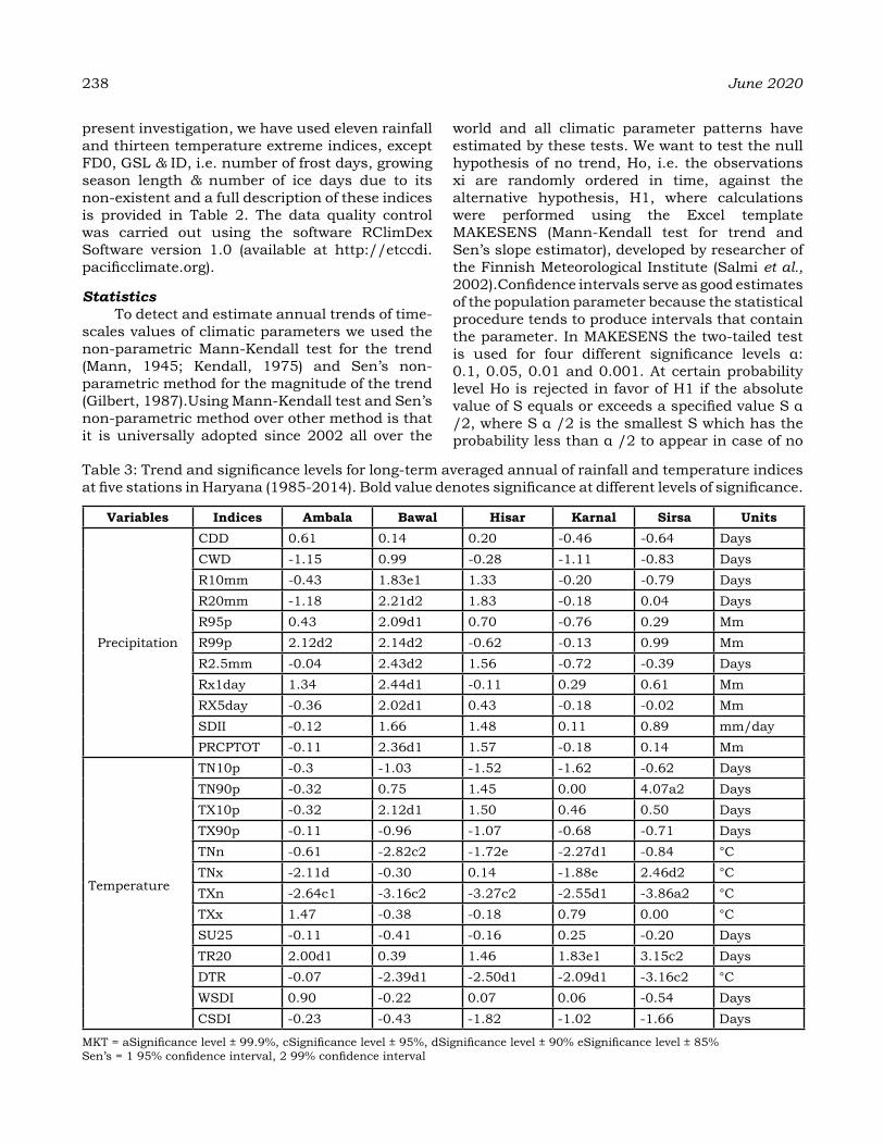
238 June 2020

present investigation, we have used eleven rainfall and thirteen temperature extreme indices, except FD0, GSL & ID, i.e. number of frost days, growing season length & number of ice days due to its non-existent and a full description of these indices is provided in Table 2. The data quality control was carried out using the software RClimDex Software version 1.0 (available at http://etccdi.pacificclimate.org).

StatisticsTo detect and estimate annual trends of time-

scales values of climatic parameters we used the non-parametric Mann-Kendall test for the trend (Mann, 1945; Kendall, 1975) and Sen’s non-parametric method for the magnitude of the trend (Gilbert, 1987).Using Mann-Kendall test and Sen’s non-parametric method over other method is that it is universally adopted since 2002 all over the

world and all climatic parameter patterns have estimated by these tests. We want to test the null hypothesis of no trend, Ho, i.e. the observations xi are randomly ordered in time, against the alternative hypothesis, H1, where calculations were performed using the Excel template MAKESENS (Mann-Kendall test for trend and Sen’s slope estimator), developed by researcher of the Finnish Meteorological Institute (Salmi et al., 2002).Confidence intervals serve as good estimates of the population parameter because the statistical procedure tends to produce intervals that contain the parameter. In MAKESENS the two-tailed test is used for four different significance levels α: 0.1, 0.05, 0.01 and 0.001. At certain probability level Ho is rejected in favor of H1 if the absolute value of S equals or exceeds a specified value S α /2, where S α /2 is the smallest S which has the probability less than α /2 to appear in case of no

Table 3: Trend and significance levels for long-term averaged annual of rainfall and temperature indices at five stations in Haryana (1985-2014). Bold value denotes significance at different levels of significance.

variables Indices ambala Bawal hisar Karnal Sirsa units

Precipitation

CDD 0.61 0.14 0.20 -0.46 -0.64 DaysCWD -1.15 0.99 -0.28 -1.11 -0.83 DaysR10mm -0.43 1.83e1 1.33 -0.20 -0.79 DaysR20mm -1.18 2.21d2 1.83 -0.18 0.04 DaysR95p 0.43 2.09d1 0.70 -0.76 0.29 MmR99p 2.12d2 2.14d2 -0.62 -0.13 0.99 MmR2.5mm -0.04 2.43d2 1.56 -0.72 -0.39 DaysRx1day 1.34 2.44d1 -0.11 0.29 0.61 MmRX5day -0.36 2.02d1 0.43 -0.18 -0.02 MmSDII -0.12 1.66 1.48 0.11 0.89 mm/dayPRCPTOT -0.11 2.36d1 1.57 -0.18 0.14 Mm

Temperature

TN10p -0.3 -1.03 -1.52 -1.62 -0.62 DaysTN90p -0.32 0.75 1.45 0.00 4.07a2 DaysTX10p -0.32 2.12d1 1.50 0.46 0.50 DaysTX90p -0.11 -0.96 -1.07 -0.68 -0.71 DaysTNn -0.61 -2.82c2 -1.72e -2.27d1 -0.84 °CTNx -2.11d -0.30 0.14 -1.88e 2.46d2 °CTXn -2.64c1 -3.16c2 -3.27c2 -2.55d1 -3.86a2 °CTXx 1.47 -0.38 -0.18 0.79 0.00 °CSU25 -0.11 -0.41 -0.16 0.25 -0.20 DaysTR20 2.00d1 0.39 1.46 1.83e1 3.15c2 DaysDTR -0.07 -2.39d1 -2.50d1 -2.09d1 -3.16c2 °CWSDI 0.90 -0.22 0.07 0.06 -0.54 DaysCSDI -0.23 -0.43 -1.82 -1.02 -1.66 Days

MKT = aSignificance level ± 99.9%, cSignificance level ± 95%, dSignificance level ± 90% eSignificance level ± 85% Sen’s = 1 95% confidence interval, 2 99% confidence interval

trend. A positive (negative) value of S indicates an upward (downward) trend.

Data quality controlThe data quality control was carried out

using the software RClimDex Software version 1.0 (available athttp://etccdi.pacificclimate.org). Time series with more than 20% missing values within an analysis period were excluded. Data quality was tested in order to label potentially wrong values, and to reject them from the analysis. Unphysical values, such as Tmax ≥ 70 °C, Tmin ≤ -50 °C, Tmax ≤ Tmin were identified and set to missing values. During the quality check procedures various errors related to data were removed such as values related to non-existing dates, both the values of daily maximum and minimum temperature were set to be missing if maximum temperature is less than minimum temperature etc. Outliers related to daily data were identified based on expert knowledge on the local climate. Outliers are the daily values that lie outside a particular range defined as unrealistic by the user. Another important issue is related to the homogeneity of dataset. Abrupt shifts in the data values can occur due to changes in station, location, environment, instrumentation or observing practices. These issues may affect the analysis of extremes. Different approaches and statistical techniques are required to detect and remove these in homogeneities. Outliers were detected and rejected if a daily value exceeded ±4 standard deviation.

reSuLtS aNd dISCuSSIoNRainfall indices: Very wet days (R95p) at

Bawal showed (Table 3) an increasing trend (2.09 mm/year) which was significant at 90% level as per Mann-Kendall test with 95% confidence level (Sen’s slope estimator). Extremely wet days (RX99p) at Ambala and Bawal had an increasing trend (2.12 and 2.14 mm/year) and was significant at 90% level with 99% confidence level. Absolute indices like maximum 1-day rainfall amount (RX1day) and maximum 5-day rainfall amount (RX5day) at Bawal station, showed an increase of 2.44 mm/year over the study period which was significant at 90% level with 95% confidence level (Table 3) and showed an increase of 2.02 mm/year over 30-years period with significance level and confidence interval matching with RX5day rainfall respectively. Threshold indices such as rainy Days (R2.5mm), number of heavy rainfall days (R10mm) and number of very heavy rainfall

days (R20mm) showed positive trend at Bawal. Analysis of annual total wet days rainfall amount (PRCPTOT) depicted that Mann-Kendall test for annual total wet days rainfall amount at Bawal showed a significant (90% significance level) increasing trend @ 2.36 mm/year with 99% confidence interval as indicated by Sen’s slope estimator. The trend for other stations was non-significant. Annual average trend for PRCPTOT in the state was 0.76mm/year. The trend for remaining four stations was not significant. Trend analysis of rainfall-related climate indices revealed that annual rainfall (PRCPTOT), consecutive wet days (CWD), and number of days with rainfall ≥ 20 mm (R20) showed a significant increasing tendency under linear regression method. Yet, underMKtest, only CWDshowed a significant rising trend. The increasing trend (non-significant under MK test) in annual rainfall at IARI is mainly attributed to excess rainfall received during monsoon season in the past 3 years. Results of Rao et al. (2004) is in agreement with the results of our study, and they found that annual rainfall increased by 33% at New Delhi during 1901–2000 Increased availability of cloud condensation nuclei might be the reason for the increase in rainfall. Further, the increased cloud condensation might be the consequence of the addition of aerosols in the atmosphere. Padmanabamurty and Bahal (1984) interpreted that enhanced rainfall amount due to urbanization has led to increased buoyancy and convection

Temperature indices: Slope and significance level for MK test of temperature and rainfall indices are furnished in Table 3. Coldest nights (TNn) at Haryana, annual averaged trend for TNn in the state was 0.165 °C/year. The Mann-Kendall and Sen’s slope estimator statics revealed Hottest nights (TNx) indices over 30-years period at Ambala, Karnal and Sirsa is -2.11, -1.88, and 2.46 °C /year respectively. Tropical nights TR20 (corresponding to nights when temperature exceeded 20 °C), had decrease (-2.00, 1.88 and 3.15, ) trend for Ambala, Karnal and Sirsa show (Table 3) was significant at as per Mann-Kendall test with confidence level (Sen’s slope estimator). Diurnal Temperature Range (DTR) (mean temperature difference of TMin and TMax) had showed (Table3) decreasing trend for all station except Ambala which was significant at as per Mann-Kendall test with confidence level (Sen’s slope estimator). The trend values for Ambala, Bawal, Hisar, Karnal and Sirsa stations were


240 June 2020

-0.07, -2.39, -2.50, -2.09 and -3.16, respectively. Annual averaged trend for DTR in the state was -0.78 °C/year. The mean temperature difference (DTR) of Tmin and Tmax analysis has shown that Tmax remained constant or slightly decrease, whereas Tmin increased faster. Trend and slope of night extremes (TR20 and TN90p) appear to have been higher than those in day extremes (TXx, TXn, TX90p, and TX10p) resulting in the decrease of day-night temperature variation which is also indicated by diurnal temperature range (DTR). Further, the value of Mann-Kendall test statistic Z and Sen’s slope test indicates that minimum temperature extremes (TNn and TXn) have stronger trend and steeper slope at all stations. Baidya et al. (2008) suggested that the negative trend in TXn in the plains might be the result of the fog episodes in winter which have become more frequent over the past decade, sometimes lasting for more than a week or even a month, which reduced the maximum temperature significantly. A study done by Ji et al. (2011) shows that negative trend in TXn in the plains could be due to emission of anthropogenic particles such as sulphate and organic carbon which scatter the incoming solar radiation and reduction in the radioactive forcing causing the decrease of temperature in plains. Another study by Ji et al. (2015) shows that negative trend in TXn in the plains could be due to increased haze occurrence and its dimming effect. The extremes related to TR20 and TN90p have increased consistently over three decadal intervals and both Mann-Kendall and Sen’s slope tests indicate that the minimum temperature extremes have the stronger trend and steeper slope. Several studies have investigated the rise in the minimum temperature in the Arabian Peninsula, which is attributed to the warming trend of changes in atmospheric circulations over the Mediterranean Sea, Indian Ocean, and Sudan (Almazroui et al., 2014 & Alsarmi and Washington, 2014). Annual DTR at Haryana showed a decreasing trend significantly (at 10% level) during the period 1985– 2014. Wild et al. (2005) drew attention on popular theory of solar dimming, and they found that amount of insolation was declining over land surface until 1990 and thereafter increment was noticed. However, they opined that Atmospheric Brown Cloud (ABCs) dimming was continued over Indian stations. Some studies also revealed that amount of solar radiation (Padma Kumari et al., 2007; Singh et al., 2012) and bright sunshine hours (Rao et al., 2004) had declined significantly

at New Delhi. Many studies were undertaken to understand the effect of increased nighttime temperature on performance of different crops. Investigation of global climate projections (Meehl et al., 2007) indicated that minimum temperature will shoot up faster than maximum temperature, and there would be greater consequences on food grain production. In general, a rise in minimum temperature increases nocturnal respiration in plants, and extra energy required for this process is obtained from stored food material which in turn affects crop yields. Cooper et al. (2008) opined that night temperature during grain development has the key role in deciding grain quality also. In thecase of rice which is a very important cereal crop in India, increase in night temperature has led to high amylase contentin rice grains (Resurreccion et al., 1977), decreasing the head rice yield (Counce et al., 2005).Wheat, another key cereal crop during winter season in India, is highly susceptible to high night temperature. According to Lobell et al. (2011), there would be yield reduction by about 10% with the increase in minimum temperature by 1 °C.

Trends for remaing indices did not depict significant trend over 30-years study period in the state.

CoNCLuSIoNSIn general, the rainfall related indices

demonstrated trend consistent with increasing rainfall over time; however, the results shown in the table 3were significant for Bawal station only. Overall, the results showed widespread significant changes in temperature trends consistent with warming, especially for those indices derived from daily minimum temperature. The minimum temperature has enhanced in terms of its maximum value as indicated by significant increase in number of warm nights and tropical nights. The results depicted in the table 3 indicated no substantial change with respect to maximum temperature values at all five selected stations. Analysis of extreme temperature events at the five locations in Haryana showed a significant increasing trend in annual minimum temperature. Because of this, diurnal temperature range is narrowing down significantly. The analysis of temperature difference (DTR) between maximum and minimum temperature had shown that maximum temperature remained constant or slight decrease, whereas minimum temperature increased faster. The minimum temperature

was enhanced in terms of its maximum value as indicated by significant increase in number of warm nights and tropical nights, which led to significant decrease in DTR. These temperature changes will have an implication on crop production especially food grain crops like rice and wheat. There would be a decrease in the rate of photosynthesis and increase in nocturnal respiration.

reFereNCe:Alexander, L.V. Zhang, X. Peterson, T.C. Caesar,

J. Gleason, B. Klein Tank, A.M.G. Haylock, M. Collins, D. Trewin, B. Rahimzadeh, F. Tagipour, A. Ambenje, P. Rupa-Kumar, K. Revadekar, J. and Griffiths, G. (2006). Global observed changes in daily climate extremes of temperature and precipitation.Geophysical Research-Atmospheres, 111: DO5109.

Almazroui, M. Islam, M.N. Dambul, R. and Jones P. (2014). Trends of temperature extremes in Saudi Arabia. International Journal of Climatology, 34: 808-826.

AlSarmi, S.H. and Washington, R. (2014). Changes in climate extremes in the Arabian Peninsula: analysis of daily data.International Journal of Climatology, 34:1329-1345.

Anonymous, (2017) “Indian Agriculture Industry: An Overview. http://www.ibef.org/industry/agriculture-india.aspx

Baidya, S.K. Shrestha, M.L. and Sheikh, M.M. (2008). Trends in daily climatic extremes of temperature and precipitation in NepaL.Journal of Hydrology and Meteorology, 5 1 pp. 38-51.

Cooper NTW, Siebenmorgen T.J. and Counce PA. (2008). Effects of night time temperature during kernel development on rice physicochemical properties. Cereal Chem. 85:276–282

Counce PA, Bryant RJ, Bergman CJ, Bautista RC, Wang YJ, Siebenmorgen TJ, Moldenhauer KAK, Meullenet JFC. (2005). Rice milling quality, grain dimensions, and starch branching as affected by high night temperatures. Cereal Chem 82:645–648

ETCCDI. (2013) Expert Team (ET) on Climate Change Detection and Indices (ETCCDI) http://etccdi.pacificclimate.org/

Gilbert, R.O. (1987). Statistical methods for environmental pollution monitoring. Van Nostrand Reinhold. New York.

Guhathakurta, P. and Rajeevan, M. (2008) Trends in the rainfall patterns over India.International Journal of Climatolog, 28: 1453–1469.

IPCC.2013, “Summary for Policymakers”. In: Climate Change (2013). The Physical Science Basis. Contribution of Working Group I to the Fifth Assessment Report of the Intergovernmental Panel on Climate Change [Stocker, T.F., D. Qin, G.-K. Plattner, M. Tignor, S. K. Allen, J. Boschung, A. Nauels, Y. Xia, V. Bex and P.M. Midgley (eds.) ]. Cambridge University Press, Cambridge, United Kingdom and New York, NY, USA.

Ji, Z.M. Kang, S.C. Cong, Z.Y. Zhang, Q.G. and Yao, Y.D. (2015). Simulation of carbonaceous aerosols over the Third Pole and adjacent regions: distribution, transportation, deposition, and climatic effects. Climate Dynamics, 45 9: 2831–2846.

Ji, Z.M. Kang, S.C. Zhang, D. Zhu, C. Wu, J. and Xu, Y. (2011). Simulation of carbonaceous aerosols over the Third Pole and adjacent regions: distribution, transportation, deposition, and climatic effects”, Climate Dynamics, 36:1633–1647.

Kendall, M. G. (1975) Rank Correlation Method. Griffin, London.

Krishna Kumar, K. Kamala, K. Rajagopalan, B. Hoerling, M.P. Eischeid, J.K. Patwardhan, S.K. Srinivasan, G. Goswami, B.N. and Nemani, R. (2010). The once and future pulse of Indian monsoonal climate.Climate Dynamic, 36:2159-2170.

Lobell DB, Schlenker W, Costa-Roberts J. (2011). Climate trends and global crop production since 1980. Science 333:616–620.

Mann, H. B. (1945). Non-parametric test against trend.Econometrica. 13: 245-259.

Meehl GA, Stocker TF, Collins WD, Gaye AJ, Gregory JM, Kitoh A, Knutti R, Murphy JM, Noda A, Raper SCB, Watterson JG, Weaver AJ, Zhao Z (2007). Global climate projections. In: Solomon S, Qin D, Manning M, Chen Z, Marquis M, Averyt KB, Tignor M, Miller HL (eds). Cambridge University Press, Cambridge.

Padma Kumari B, Londhe AL, Daniel S, Jadhav DB. (2007). Observational evidence of solar dimming: offsetting surface warming over India. Geophys Res Lett 34:L21810. https://doi.org/10.1029/2007GL031133


242 June 2020

Wild M, Gilgen H, Roesch A, Ohmura A, Long CN, Dutton EG, Forgan B, Kallis A, Russak V, Tsvetkov A (2005) From dimming to brightening: decadal changes in solar radiation at Earth’s surface. Science 308:847–850.

Padmanabamurty B, Bahal H.D . (1984). Isothermal and isohyetal patterns of Delhi as a sequel of urbanization. Mausam 35 (4) :539–540.

Pant, G. B. and Rupa Kumar, K. (1997) Climates of South Asia, John Wiley. Chichester, pp. 320.

Parthasarthy, B. (1984). Inter-annual and long term variability of Indian summer monsoon rainfall. The proceedings of the Indian Academy of Sciences.Earth and Planetary Sciences, 93: 371- 385.

Planning Commission of India, Agro-climatic Zones of India, (1989). pp. 1985–1990.

Rao GSP, Jaswal AK, Kumar . (2004). Effect of urbanization on meteorological parameters. Mausam 55 (3) :429–440.

Resurreccion AP, Hara T, Juliano BO, Yoshida S. (1977). Effect of temperature during ripening on grain quality of rice. Soil Sci Plant Nutr 23:109–112.

Rupa Kumar, K. Krishna Kumar, K. and Pant, G. B. (1994). Diurnal asymmetry of surface

temperature trends over India. Geophysical Research letter 21:677-680.

Salmi, T., Maatta, A., Anttila, P., Ruoho-Airola, T., Amnell, T. (2002). Publications on air quality. No 31. Detecting trends of annual values of atmospheric pollutants by the Mann-Kendall test and Sen’s slope estimates. Finnish Meteorological Institute Helsinki, Finland.

Shrestha, A.B. Bajracharya, S.R. Sharma, A.R. Duo, C. and Kulkarnid, A. (2016).Observed trends and changes in daily temperature and precipitation extremes over the Koshi river basin 1975-2010. International Journal of Climatology.DOI: 10.1002/joc.4761.

Singh J, Bhattacharya BK, Kumar M. (2012). Solar radiation and evaporation trend over India. International Association for Urban Climate Newsletter 2:160–165.

Wild, M., Gilgen H., Roesch A., Ohmura A., Charles N. L., Ellsworth G.D., Forgan B., Kallis A., Russak V., Tsvetkov A. (2005). From dimming to brightening: Decadal changes in surface solar radiation.Science, 308: 847-850.

Zhang X, Yang F. (2004). RClimDex (1.0) user manual. Climate Research Branch, Environment Canada, Ontario 23p.

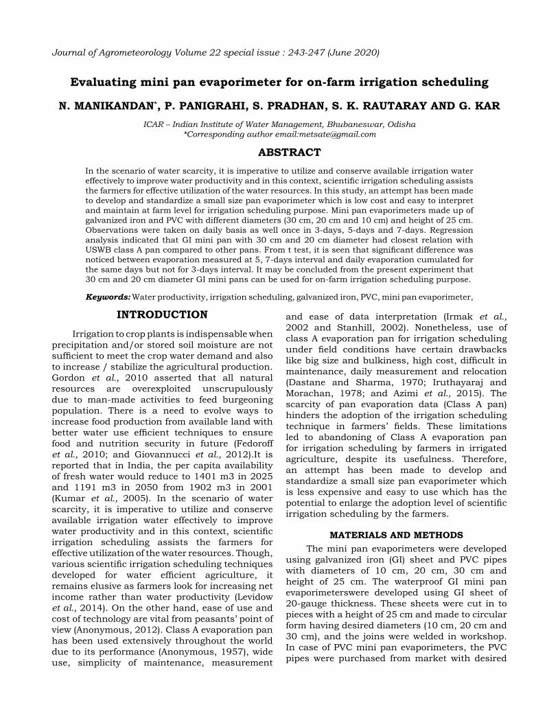
evaluating mini pan evaporimeter for on-farm irrigation scheduling

N. MaNIKaNdaN*, P. PaNIgrahI, S. PradhaN, S. K. rautaraY aNd g. KarICAR – Indian Institute of Water Management, Bhubaneswar, Odisha

*Corresponding author email:[email protected]

aBStraCtIn the scenario of water scarcity, it is imperative to utilize and conserve available irrigation water effectively to improve water productivity and in this context, scientific irrigation scheduling assists the farmers for effective utilization of the water resources. In this study, an attempt has been made to develop and standardize a small size pan evaporimeter which is low cost and easy to interpret and maintain at farm level for irrigation scheduling purpose. Mini pan evaporimeters made up of galvanized iron and PVC with different diameters (30 cm, 20 cm and 10 cm) and height of 25 cm. Observations were taken on daily basis as well once in 3-days, 5-days and 7-days. Regression analysis indicated that GI mini pan with 30 cm and 20 cm diameter had closest relation with USWB class A pan compared to other pans. From t test, it is seen that significant difference was noticed between evaporation measured at 5, 7-days interval and daily evaporation cumulated for the same days but not for 3-days interval. It may be concluded from the present experiment that 30 cm and 20 cm diameter GI mini pans can be used for on-farm irrigation scheduling purpose.

Keywords: Water productivity, irrigation scheduling, galvanized iron, PVC, mini pan evaporimeter,

INtroduCtIoN

Irrigation to crop plants is indispensable when precipitation and/or stored soil moisture are not sufficient to meet the crop water demand and also to increase / stabilize the agricultural production. Gordon et al., 2010 asserted that all natural resources are overexploited unscrupulously due to man-made activities to feed burgeoning population. There is a need to evolve ways to increase food production from available land with better water use efficient techniques to ensure food and nutrition security in future (Fedoroff et al., 2010; and Giovannucci et al., 2012).It is reported that in India, the per capita availability of fresh water would reduce to 1401 m3 in 2025 and 1191 m3 in 2050 from 1902 m3 in 2001 (Kumar et al., 2005). In the scenario of water scarcity, it is imperative to utilize and conserve available irrigation water effectively to improve water productivity and in this context, scientific irrigation scheduling assists the farmers for effective utilization of the water resources. Though, various scientific irrigation scheduling techniques developed for water efficient agriculture, it remains elusive as farmers look for increasing net income rather than water productivity (Levidow et al., 2014). On the other hand, ease of use and cost of technology are vital from peasants’ point of view (Anonymous, 2012). Class A evaporation pan has been used extensively throughout the world due to its performance (Anonymous, 1957), wide use, simplicity of maintenance, measurement

and ease of data interpretation (Irmak et al., 2002 and Stanhill, 2002). Nonetheless, use of class A evaporation pan for irrigation scheduling under field conditions have certain drawbacks like big size and bulkiness, high cost, difficult in maintenance, daily measurement and relocation (Dastane and Sharma, 1970; Iruthayaraj and Morachan, 1978; and Azimi et al., 2015). The scarcity of pan evaporation data (Class A pan) hinders the adoption of the irrigation scheduling technique in farmers’ fields. These limitations led to abandoning of Class A evaporation pan for irrigation scheduling by farmers in irrigated agriculture, despite its usefulness. Therefore, an attempt has been made to develop and standardize a small size pan evaporimeter which is less expensive and easy to use which has the potential to enlarge the adoption level of scientific irrigation scheduling by the farmers.

MaterIaLS aNd MethodSThe mini pan evaporimeters were developed

using galvanized iron (GI) sheet and PVC pipes with diameters of 10 cm, 20 cm, 30 cm and height of 25 cm. The waterproof GI mini pan evaporimeterswere developed using GI sheet of 20-gauge thickness. These sheets were cut in to pieces with a height of 25 cm and made to circular form having desired diameters (10 cm, 20 cm and 30 cm), and the joins were welded in workshop. In case of PVC mini pan evaporimeters, the PVC pipes were purchased from market with desired


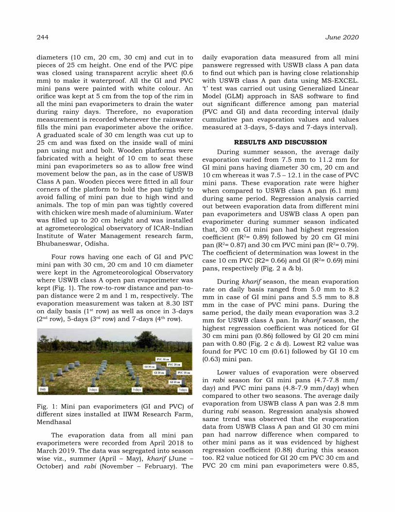
244 June 2020

diameters (10 cm, 20 cm, 30 cm) and cut in to pieces of 25 cm height. One end of the PVC pipe was closed using transparent acrylic sheet (0.6 mm) to make it waterproof. All the GI and PVC mini pans were painted with white colour. An orifice was kept at 5 cm from the top of the rim in all the mini pan evaporimeters to drain the water during rainy days. Therefore, no evaporation measurement is recorded whenever the rainwater fills the mini pan evaporimeter above the orifice. A graduated scale of 30 cm length was cut up to 25 cm and was fixed on the inside wall of mini pan using nut and bolt. Wooden platforms were fabricated with a height of 10 cm to seat these mini pan evaporimeters so as to allow free wind movement below the pan, as in the case of USWB Class A pan. Wooden pieces were fitted in all four corners of the platform to hold the pan tightly to avoid falling of mini pan due to high wind and animals. The top of min pan was tightly covered with chicken wire mesh made of aluminium. Water was filled up to 20 cm height and was installed at agrometeorological observatory of ICAR–Indian Institute of Water Management research farm, Bhubaneswar, Odisha.

Four rows having one each of GI and PVC mini pan with 30 cm, 20 cm and 10 cm diameter were kept in the Agrometeorological Observatory where USWB class A open pan evaporimeter was kept (Fig. 1). The row-to-row distance and pan-to-pan distance were 2 m and 1 m, respectively. The evaporation measurement was taken at 8.30 IST on daily basis (1st row) as well as once in 3-days (2nd row), 5-days (3rd row) and 7-days (4th row).

Fig. 1: Mini pan evaporimeters (GI and PVC) of different sizes installed at IIWM Research Farm, Mendhasal

The evaporation data from all mini pan evaporimeters were recorded from April 2018 to March 2019. The data was segregated into season wise viz., summer (April – May), kharif (June – October) and rabi (November – February). The

daily evaporation data measured from all mini panswere regressed with USWB class A pan data to find out which pan is having close relationship with USWB class A pan data using MS-EXCEL. ‘t’ test was carried out using Generalized Linear Model (GLM) approach in SAS software to find out significant difference among pan material (PVC and GI) and data recording interval (daily cumulative pan evaporation values and values measured at 3-days, 5-days and 7-days interval).

reSuLtS aNd dISCuSSIoNDuring summer season, the average daily

evaporation varied from 7.5 mm to 11.2 mm for GI mini pans having diameter 30 cm, 20 cm and 10 cm whereas it was 7.5 – 12.1 in the case of PVC mini pans. These evaporation rate were higher when compared to USWB class A pan (6.1 mm) during same period. Regression analysis carried out between evaporation data from different mini pan evaporimeters and USWB class A open pan evaporimeter during summer season indicated that, 30 cm GI mini pan had highest regression coefficient (R2= 0.89) followed by 20 cm GI mini pan (R2= 0.87) and 30 cm PVC mini pan (R2= 0.79). The coefficient of determination was lowest in the case 10 cm PVC (R2= 0.66) and GI (R2= 0.69) mini pans, respectively (Fig. 2 a & b).

During kharif season, the mean evaporation rate on daily basis ranged from 5.0 mm to 8.2 mm in case of GI mini pans and 5.5 mm to 8.8 mm in the case of PVC mini pans. During the same period, the daily mean evaporation was 3.2 mm for USWB class A pan. In kharif season, the highest regression coefficient was noticed for GI 30 cm mini pan (0.86) followed by GI 20 cm mini pan with 0.80 (Fig. 2 c & d). Lowest R2 value was found for PVC 10 cm (0.61) followed by GI 10 cm (0.63) mini pan.

Lower values of evaporation were observed in rabi season for GI mini pans (4.7-7.8 mm/day) and PVC mini pans (4.8-7.9 mm/day) when compared to other two seasons. The average daily evaporation from USWB class A pan was 2.8 mm during rabi season. Regression analysis showed same trend was observed that the evaporation data from USWB Class A pan and GI 30 cm mini pan had narrow difference when compared to other mini pans as it was evidenced by highest regression coefficient (0.88) during this season too. R2 value noticed for GI 20 cm PVC 30 cm and PVC 20 cm mini pan evaporimeters were 0.85,

0.76 and 0.73, respectively (Fig. 2 e & f).

It was noticed that the evaporation rate of GI and PVC mini pans (irrespective of diameter) were higher than USWB class A pan in all three seasons. The difference in evaporation progressively increased from bigger size mini pan (30 cm) to smaller size mini pan (10 cm) and smaller pan registered higher evaporation and vice versa. Owing to presence of low volume of water in smaller pans, it got heated quickly than bigger pans where the volume of water was more. In addition, the saturated water vapour present above the air column of smaller pans can become unsaturated even at lower wind speed and vapour pressure

deficit would be more and hence evaporation rate when compared to bigger pans. Azimi et al., 2015 also demonstrated that pan with smaller diameter registered higher evaporation rate and the evaporation data reliability reduced from bigger diameter pan to smaller one when compared to USWB class A pan.It was also observed that the evaporation data was more for PVC mini pans than the GI mini pans. From the ‘t’ test it was noticed that the evaporation data recorded from GI and PVC mini pans were significantly different (Table 1).This could be due to thermal properties of PVC material like higher specific heat and lower thermal conductivity (0.24 cal gm-1 °C and 0.13 - 0.17 W m-1 °K) than the GI material (0.11cal

Fig. 2 (a-f). Scatter graph of evaporation data from GI, PVC mini pans and USWB pan in different seasons

Vol. 22, Special Issue MANIKANDAN et al. 245

246 June 2020

gm-1 °C and 60 W m-1 °K).

The statistical analysis between the evaporation measured at 3, 5 and 7-days interval and daily evaporation cumulated for 3, 5 and 7-days revealed that there was significant difference for 5-days and 7-days direct and cumulated values (Table 1). However, no significant difference was observed for 3-days. It is also noticed that the evaporation value taken directly at 3, 5 and 7-days interval had less value than daily cumulated values for the same days. One reason could be the measurement error in daily observation than the observation taken at 3, 5 and 7-days interval.The other reason might be the water depth was lesser in the mini pans kept under 3, 5 and 7-days interval than the mini pans under daily measurement except the days when daily measurement and 3-days / 5-days / 7-days measurement coincided. The reduction in water depth in the pan decreased the evaporation rate due to the reduced effect of wind speed that blew over the water surface of pan due shelter effect of the rim of the pan (Chia Ren Chu et al., 2010).

Marston, 1961;Davis, 1963 and Simmone et al., 1992 also tested mini evaporimeters (made up of different material and smaller size than USWB class A pan) and demonstrated that smaller size pan evaporimeters can be considered for irrigation scheduling. Therefore, it is clear from this study that the GI mini pan with 30 and 20 cm diameter can be used for on-farm irrigation scheduling as they were closest to USWB class A pan. However, the performance of these pans needs to tested in irrigation scheduling experiments at different locations.

CoNCLuSIoNSThe present study was undertaken to develop

a low cost, easy to use and smaller size evaporation pan for on-farm irrigation scheduling purpose. Regression analysis revealed that among the mini pans fabricated using GI and PVC with different diameters (30 cm, 20 cm and 10 cm) and height of 25 cm, GI mini pan with 30 cm and 20 cm diameter had closest relation with USWB class A pan. From t test, it was observed that the evaporation from PVC and GI mini pan were significantly different due to thermal and radiative characters of these pans. It was also noticed that significant difference exists between evaporation measured at 5-days, 7-days interval and daily evaporation cumulated for the same days. No significant difference was seen for evaporation measured at 3-days interval. From this study, it may be concluded that GI mini pans of 30 cm and 20 cm diameter measured at either daily or 3-days interval can be used for on-farm irrigation scheduling purpose. However, the performance of these mini pans will be tested in crop experiment involving irrigation scheduling treatments.

reFereNCeSAnonymous. (1957). “Abridged final Report of

the second session of the Commission for Instruments and Methods of Observation (CIMO) ”. held at Paris during June 18 – July 6, 1957. WMO No 64, RP 26, World Meteorological Organization, Geneva, Switzerland, 79p.

Anonymous. (2012). “Crop Yield response to water”. FAO Irrigation and Drainage Paper 66. Food and Agriculture Organization,

Table 1: ‘t’ test results for GI and PVC mini pans

Parameter Mean (mm) Pan materialPVC 31.24aGI 29.32b

Cumulated evaporation value vs direct evaporation valueDaily value cumulated for 7 days 41.73aValue taken at 7 days interval 38.32bDaily value cumulated for 5 days 31.88cValue taken at 5 days interval 30.00dDaily value cumulated for 3 days 20.38eValue taken at 3 days interval 19.38eAlphabets (mentioned as superscript in mean values) having same letters are not significantly different

Geneva, Rome, 500p.Azimi, M.A., Mansti, M.J., Motahari, A.G., Karami,

A. and Rostami, K. (2015). Determining hourly evaporation measurement accuracy of small pans in comparison with Class-A pan. Asian Journal of Applied Sciences, 3 (6) : 844-847

Chin Ren Chu., Ming Hsu Li., Yi Ying Chen and Yi HsinKuo. (2010). A wind tunnel experiment on the evaporation rate of class A evaporation pan. J. Hydrology. 381: 221-224

Dastane, N. G. and Sharma, H C. (1970). Use of sunken screened pan evaporimeters in irrigation practices. Indian Journal of Agronomy, 15: 271-276

Davis, J.R. (1963). Relationship of can evaporation to pan evaporation and evapotranspiration. Journal of Geophysical Research, 68 (20) : 5711-5718

Fedoroff, N.V., Battisti, D.S., Beachy, R.N., Cooper, P.J.M., Fischhoff, D.A., Hodges, C.N., Knauf, V.C., Lobell, D., Mazur, B.J., Molden, D., Reynolds, M.P., Ronald, P.C., Rosegrant, M.W., Sanchez, P.A., Vonshak, A. and Zhu, J.K. (2010). Radically rethinking agriculture for the 21st century. Science 327, 833-834.

Giovannucci, D., Scherr, S.J., Nierenberg, D., Hebebrand, C., Shapiro, J., Milder, J. and Wheeler, K. (2012). “Food and Agriculture: The Future of Sustainability: Sustainable Development in the 21st Century”. UN Department of Economic and Social Affairs, Division of Sustainable Development. New York.

Gordon, L. J., Finlayson, C. M. and Falkenmark, M. (2010). Managing water in agriculture

for food production and other ecosystem services. Agricultural Water Management, 97: 512–519.

Irmak, S., Haman, D.Z. and Jones, J.W. (2002). Evaluation of Class A pan coefficients for estimating reference evapotranspiration in humid location. Journal of Irrigation and Drainage Engineering, 128 (3) : 153-159

Iruthayaraj, M.R. and Morachan, Y.B. (1978). Relationship between evaporation from different evaporimeters and meteorological parameters. Agricultural Meteorology, 19: 93-100

Kumar, R., Singh, R.D. and Sharma, K.D. (2005). Water resources of India. Current Science, 89 (5) :794 – 811

Levidow, L., Zaccaria, D., Maia, R., Vivas, E., Todorovic, M. and Scardigno, A. (2014). Improving water-efficient irrigation: Prospects and difficulties of innovative practices. Agricultural Water Management, 146: 84-94

Marston, R.B. (1961). Substitution of small cans for weather bureau pans in measuring evaporation. Journal of Geophysical Research, 66 (2) : 657-659

Simonne, E., Mills, H. A. and Smittle, D.A. (1992). A simple method to measure on-farm pan evaporation for scheduling irrigation. Hort Technology, 2 (3) : 392-393

Stanhill, G. (2002). Is the Class A evaporation pan still the most practical and accurate meteorological method for determining irrigation water requirements? Agric For Meteorol 112:233–236

Vol. 22, Special Issue MANIKANDAN et al. 247

CroP PLaNNINg BaSed oN Water BaLaNCe aPProaCh IN KeraLa*harItharaJ S. aNd B. aJIthKuMar

Department of Agricultural Meteorology, College of Horticulture, Kerala Agricultural University, Thrissur-680656

*Corresponding author’s email: [email protected]

aBStraCtWeather data were collected from three agro-climatic zones of Kerala from the year 2000 to 2014. Using these data as input, reference crop evapotranspiration (ETo) values were obtained with the help of CROPWAT software. With these ETo values of each zone along with the rainfall data, weekly thornthwaite water balance was calculated using the software Weather Cock. From the output obtained from Weather Cock, Potential Evapotranspiration (PET) and Moisture Availability Index (MAI) were used to plot the graph against each year. The rainfall deviation is calculated and plotted against corresponding years to determine the excess rainfall year and deficit year. It was observed that a high PET value is obtained in the Central Zone (Thrissur, Vellanikkara) during 2003 which was a rainfall deficient year for that zone and low PET was observed in 2013 which is an excess rainfall year. In the case of Southern Zone (Trivandrum, Vellayani), 2007 and 2014 observed as excess rainfall years with low PET values and high MAI. Pilicode which comes in Kasargod (Northern Zone) showing a low PET value in the year 2004 during which sufficient rainfall was received and also 2007 and 2010 were observed as the excess rainfall years for the zone. Crop planning according to the moisture availability and chances of rainfall affect the growing period of crops and finally the yield. During high rainfall season, crops with higher water requirements can be used for planting whereas in low rainfall conditions the available moisture will be lesser and the duration of the crop will be affected. Therefore, it is better to grow crops like millets which require less moisture for its growth during these low rainfall conditions.

Keywords: MAI, crop plan, PET, CROPWAT

INtroduCtIoN

The important sector of Indian economy is agriculture. The Indian agriculture sector accounts for 18 % of India’s gross domestic product (GDP) and more than 50% of the population depend on agriculture as it provides employment to 50% of the countries workforce (India Economic Survey, 2018). Agriculture has to face various challenges such as irrigation water management, land allocation, climate changes, human and other resources. Weather plays an important role in agricultural production. It has a profound influence on growth, development and yields of the crop; on the incidence of pests and diseases; on water needs; and on fertilizer requirements Even on a climatological basis, weather factors cause spatial variations in an area at a given time, temporal variations for a given place, and year to year variations for a given place and time.

Crop planning help to utilize the minimum resources like water and land to get the maximum profit and productivity (Georgiou and Papamichail, 2008). Presently, less than 25% of today’s farmers have a detailed crop plan for their farms. Crop planning according to the moisture availability

as well as chances of rainfall affect the growing period of crops and finally yield (Sethi et al., 2002). The study aimed to develop crop planning for three agro-climatic zones of Kerala based on past 14 years data.

MaterIaLS aNd MethodSThe input weather data consisting of

maximum temperature, minimum temperature, rainfall, bright sunshine hours, relative humidity and wind speed that required run CROPWAT model (Molua and Lambi, 2006) were collected from three agroclimatic zones viz. Southern zone (Vellayani, Trivandrum), Central zone (Vellanikkara, Thrissur) and Northern zone (Pilicode, Palakkad) of Kerala from the year 2000 to 2014. Reference crop evapotranspiration (ETo) values were obtained with the help of CROPWAT software by using weather data except for rainfall data as input for all these zones. The ETo values along with the rainfall data were used to calculate weekly thornthwaite water balance using the software Weather Cock. From the output Potential Evapotranspiration (PET) and Moisture Adequacy Index (MAI) were used to plot the graph against each year. Correlation analysis was carried out


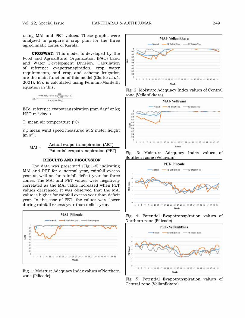
using MAI and PET values. These graphs were analyzed to prepare a crop plan for the three agroclimatic zones of Kerala.

CroPWat: This model is developed by the Food and Agricultural Organization (FAO) Land and Water Development Division. Calculation of reference evapotranspiration, crop water requirements, and crop and scheme irrigation are the main function of this model (Clarke et al., 2001). ETo is calculated using Penman-Monteith equation in this.

ETo: reference evapotranspiration (mm day-1 or kg H2O m-2 day-1)

T: mean air temperature (°C)

u2: mean wind speed measured at 2 meter height (m s-1).

MAI =Actual evapo-transpiration (AET) Potential evapotranspiration (PET)

reSuLtS aNd dISCuSSIoNThe data was presented (Fig:1-6) indicating

MAI and PET for a normal year, rainfall excess year as well as for rainfall deficit year for three zones. The MAI and PET values were negatively correlated as the MAI value increased when PET values decreased. It was observed that the MAI value is higher for rainfall excess year than deficit year. In the case of PET, the values were lower during rainfall excess year than deficit year.

Fig. 1: Moisture Adequacy Index values of Northern zone (Pilicode)

Fig. 2: Moisture Adequacy Index values of Central zone (Vellanikkara)

Fig. 3: Moisture Adequacy Index values of Southern zone (Vellayani)

Fig. 4: Potential Evapotranspiration values of Northern zone (Pilicode)

Fig. 5: Potential Evapotranspiration values of Central zone (Vellanikkara)

Vol. 22, Special Issue HARITHARAJ & AJITHKUMAR 249

250 June 2020

Fig. 6: Potential Evapotranspiration values of Southern zone (Vellayani)

From the graph it was clear that in the Southern zone during kharif (Virippu) season, the MAI values were coinciding with the normal. In rabi (Mundakan) season, the Southern zone was not much affected by the rainfall deficit condition since it experienced a bimodal rainfall distribution. More emphasis is given to the summer season in Southern zone since more evaporation and low MAI were experienced in that zone which adversely affected the major crops.

In the Central zone, kharif season not much affected as in the case of the Southern zone. But during rabi season, low MAI value and high PET value were experienced. Therefore, attention should be given by providing optimum irrigation so that the crops can be saved from major damaged situations. Otherwise, planning can be done so that the maturity stage of the crop will coincide with the low MAI and high PET values.

In Northern zone also, there was no water scarcity during kharif season whereas rabi was more affected by the low MAI values and high PET values because, northern zone receiving unimodal way of rainfall. Therefore, the focus might be given on the Mundakan season as the Virippu and Mundakan seasons are the two major crop growing seasons of Kerala.

In Puncha (summer) season, the MAI value was much more decreased (<0.7) for all three zones and the central zone experiencing a long

period of lower MAI value which will adversely affect the major crops (Jadhav et al., 2015).

CoNCLuSIoNKharif season crops were not much affected

by the climatic conditions prevailed in the three agroclimatic zones. With more irrigation during the Mundakan season, crop cultivation can help to get a good economic returns. During the period of high MAI value and low PET more water required crops like rice, vegetables etc. can be grown in order to use available water. In dry spell conditions crop planning be redesigned in a way either the maturity stage of the crop coinciding with low MAI and high PET value, or we can plant crops like millets, grams etc. which require a low moisture availability for its growth.

reFereNCe Clarke, D., Smith, M., and El-Askari, K. 2001.

CropWat for Windows: user guide. IHE.Georgiou, P. E. and Papamichail, D. M. 2008.

Optimization model of an irrigation reservoir for water allocation and crop planning under various weather conditions. Irrigation science, 26 (6) : 487-504.

GOI [Government of India]. 2018. Economic survey 2018 [online]. Available: https://www.indiabudget.gov.in/economicsurvey.

Jadhav, M. G., Aher, H. V., Jadhav, A. S., and Gote, G. N. (2015). Crop Planning Based on Moisture Adequacy Index (MAI) of Different Talukas of Aurangabad District of Maharashtra. Indian J. Dryland Agric. Res. Develop. 30 (1) : 101.

Molua, E. L. and Lambi, C. M. 2006. Assessing the impact of climate on crop water use and crop water productivity: The CROPWAT analysis of three districts in Cameroon. University of Pretoria: Pretoria, South Africa, p.44.

Sethi, L. N., Kumar, D. N., Panda, S. N., and Mal, B. C. 2002. Optimal crop planning and conjunctive use of water resources in a coastal river basin. Water resources management, 16 (2) : 145-169.

Impact of el Niño–Southern oscillation on rainfall and Major Kharif Crops Production of vidarbha region

Y. e. KadaM1; K. K. daKhore2; a. S. Jadhav3; d. P. WaSKar4 ; P. vIJaYa KuMar5 aNd NIteSh aWaSthI6

1Senior Research Fellow, FASAL, VNMKV, Parbhani2Agrometeorologist, AICRP on Agrometeorology, VNMKV, Parbhani

3Deputy Director of Research, VNMKV, Parbhani4Director of Research, VNMKV, Parbhani

5Project Coordinator, AICRP on Agrometeorology, CRIDA, Hyderabad6Senior Research Fellow, IMD, New Delhi

aBStraCtThe impact of El Niño–southern oscillation (ENSO) on rainfall and major Kharif crop production was analysed for the period 1985-2017. For this study daily rainfall and crop yield data was collected from India Meteorological Department, Pune and Department of Agriculture, Maharashtra respectively. The Impact of rainfall on productivity of major Kharif crops under different categories of El Niño episode was studied in different districts of Vidarbha region. The rainfall during summer, monsoon, post monsoon and winter seasons were 53.4, -6.1%, 1.1% and 41.2% less respectively during El Niño years compared to normal years in Amravati division. Similarly, in the Nagpur division SW monsoon was 33.3%, 12.2%, 12.3% and 68.3% less during summer, monsoon, post-monsoon and winter seasons respectively during El Niño years. The result showed that the SW monsoon rainfall and annual rainfall was less during El Niño years as compared to normal years. During El Niño years, rainfall in Amravati division was more in June and August and less in July and September compared to normal years. On the contrary, Nagpur district received less rainfall in all the months during El Niño years. Influence of El Niño episodes on productivity of different major Kharif crops of Vidarbha was highly influenced by El Niño episodes. In majority of the districts, Kharif crops produced tended to decline during strong El Niño years as compared to Weak and Moderate El Niño years. Among the different categories of El Niño, strong events exerted a more negative impact on major Kharif crop productivity in all the districts of Vidarbha region.

Key word: Rainfall (mm), Season, ENSO and productivity.

INtroduCtIoN

Agriculture is sensitive to short term changes in weather and to seasonal, annual and long term variations in climate. Monsoon rainfall is a key factor in determining the agricultural productivity. Among the climatic factors influencing Indian monsoons, El Niño is one global phenomenon found to have a strong bearing on the intensity of monsoon rainfall variations. Understanding the impact of El Niño-Southern Oscillation (ENSO) on the monsoon rainfall at regional scales is important to balance agricultural production. Over the years, the term “El Niño” has come to be reserved for these exceptionally strong warm intervals that not only disrupt the normal lives of the fishermen, but also bring heavy rains (Prasad et al. 2014) to the equatorial coast of South America, and convective storms and hurricanes to the central Pacific region. It is worth highlighting that although records of El Niño are available

from the 19th century, the correlation between the monsoon rainfall and El Niño seems to have strengthened only in the recent past. Since 1950, there were 23 El Niño years and only 13 drought years and three of these droughts were in non-El Niño years. However, since 1980, all Indian droughts happened in the years of El Niño, but all El Niño year did not result in droughts. The occurrence of El Niño or La Niña may affect the food grain production. Most of the El Niño occurred have brought a reduction in food grain production and the occurrence of La Niña have brought an increase in the food grain production in many cases (Selvaraju, 2003). Transpiration through plant parts, utilizes a lot of moisture from the soil. Hence, the amount of rainfall received during the life cycle of crop plays an important role in the final product of the crop (Mehta et al. 2002).

MaterIaLS aNd MethodSThe district-wise daily rainfall data for


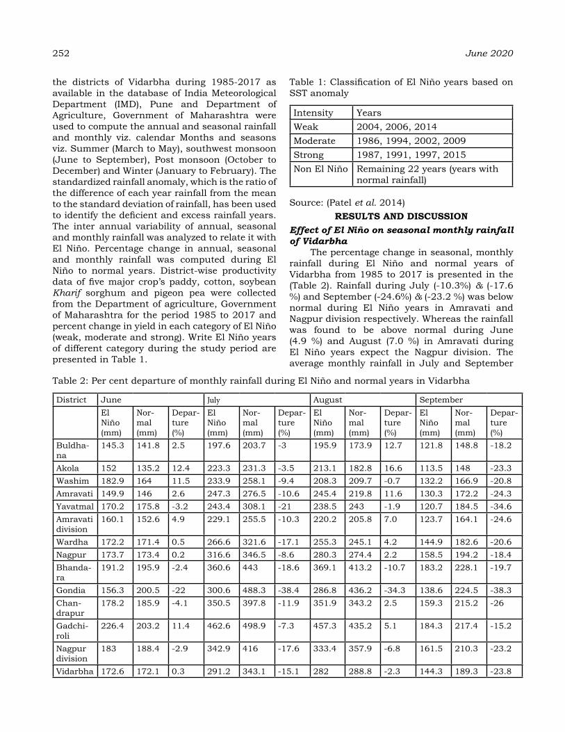
252 June 2020

the districts of Vidarbha during 1985-2017 as available in the database of India Meteorological Department (IMD), Pune and Department of Agriculture, Government of Maharashtra were used to compute the annual and seasonal rainfall and monthly viz. calendar Months and seasons viz. Summer (March to May), southwest monsoon (June to September), Post monsoon (October to December) and Winter (January to February). The standardized rainfall anomaly, which is the ratio of the difference of each year rainfall from the mean to the standard deviation of rainfall, has been used to identify the deficient and excess rainfall years. The inter annual variability of annual, seasonal and monthly rainfall was analyzed to relate it with El Niño. Percentage change in annual, seasonal and monthly rainfall was computed during El Niño to normal years. District-wise productivity data of five major crop’s paddy, cotton, soybean Kharif sorghum and pigeon pea were collected from the Department of agriculture, Government of Maharashtra for the period 1985 to 2017 and percent change in yield in each category of El Niño (weak, moderate and strong). Write El Niño years of different category during the study period are presented in Table 1.

Table 1: Classification of El Niño years based on SST anomaly

Intensity YearsWeak 2004, 2006, 2014Moderate 1986, 1994, 2002, 2009Strong 1987, 1991, 1997, 2015Non El Niño Remaining 22 years (years with

normal rainfall) Source: (Patel et al. 2014)

reSuLtS aNd dISCuSSIoNEffect of El Niño on seasonal monthly rainfall of Vidarbha

The percentage change in seasonal, monthly rainfall during El Niño and normal years of Vidarbha from 1985 to 2017 is presented in the (Table 2). Rainfall during July (-10.3%) & (-17.6 %) and September (-24.6%) & (-23.2 %) was below normal during El Niño years in Amravati and Nagpur division respectively. Whereas the rainfall was found to be above normal during June (4.9 %) and August (7.0 %) in Amravati during El Niño years expect the Nagpur division. The average monthly rainfall in July and September

Table 2: Per cent departure of monthly rainfall during El Niño and normal years in Vidarbha

District June July August SeptemberEl Niño (mm)

Nor-mal (mm)

Depar-ture (%)

El Niño (mm)

Nor-mal (mm)

Depar-ture (%)

El Niño (mm)

Nor-mal (mm)

Depar-ture (%)

El Niño (mm)

Nor-mal (mm)

Depar-ture (%)

Buldha-na

145.3 141.8 2.5 197.6 203.7 -3 195.9 173.9 12.7 121.8 148.8 -18.2

Akola 152 135.2 12.4 223.3 231.3 -3.5 213.1 182.8 16.6 113.5 148 -23.3Washim 182.9 164 11.5 233.9 258.1 -9.4 208.3 209.7 -0.7 132.2 166.9 -20.8Amravati 149.9 146 2.6 247.3 276.5 -10.6 245.4 219.8 11.6 130.3 172.2 -24.3Yavatmal 170.2 175.8 -3.2 243.4 308.1 -21 238.5 243 -1.9 120.7 184.5 -34.6Amravati division

160.1 152.6 4.9 229.1 255.5 -10.3 220.2 205.8 7.0 123.7 164.1 -24.6

Wardha 172.2 171.4 0.5 266.6 321.6 -17.1 255.3 245.1 4.2 144.9 182.6 -20.6Nagpur 173.7 173.4 0.2 316.6 346.5 -8.6 280.3 274.4 2.2 158.5 194.2 -18.4Bhanda-ra

191.2 195.9 -2.4 360.6 443 -18.6 369.1 413.2 -10.7 183.2 228.1 -19.7

Gondia 156.3 200.5 -22 300.6 488.3 -38.4 286.8 436.2 -34.3 138.6 224.5 -38.3Chan-drapur

178.2 185.9 -4.1 350.5 397.8 -11.9 351.9 343.2 2.5 159.3 215.2 -26

Gadchi-roli

226.4 203.2 11.4 462.6 498.9 -7.3 457.3 435.2 5.1 184.3 217.4 -15.2

Nagpur division

183 188.4 -2.9 342.9 416 -17.6 333.4 357.9 -6.8 161.5 210.3 -23.2

Vidarbha 172.6 172.1 0.3 291.2 343.1 -15.1 282 288.8 -2.3 144.3 189.3 -23.8

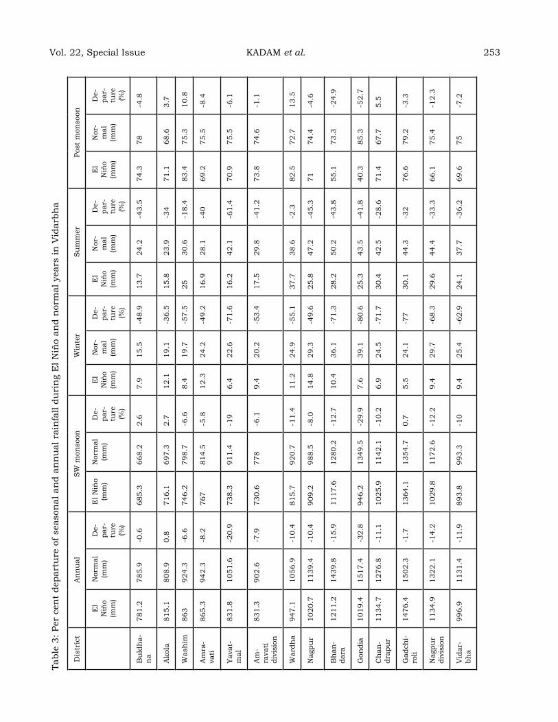
Tabl

e 3:

Per

cen

t de

part

ure

of s

easo

nal

an

d an

nu

al r

ain

fall

duri

ng

El N

iño

and

nor

mal

yea

rs in

Vid

arbh

a

Dis

tric

tA

nn

ual

SW

mon

soon

Win

ter

Su

mm

erPo

st m

onso

on

El

Niñ

o (m

m)

Nor

mal

(m

m)

De-

par-

ture

(%

)

El N

iño

(mm

) N

orm

al

(mm

) D

e-pa

r-tu

re

(%)

El

Niñ

o (m

m)

Nor

-m

al

(mm

)

De-

par-

ture

(%

)

El

Niñ

o (m

m)

Nor

-m

al

(mm

)

De-

par-

ture

(%

)

El

Niñ

o (m

m)

Nor

-m

al

(mm

)

De-

par-

ture

(%

)

Bu

ldh

a-n

a78

1.2

785.

9-0

.668

5.3

668.

22.

67.

915

.5-4

8.9

13.7

24.2

-43.

574

.378

-4.8

Ako

la81

5.1

808.

90.

871

6.1

697.

32.

712

.119

.1-3

6.5

15.8

23.9

-34

71.1

68.6

3.7

Was

him

863

924.

3-6

.674

6.2

798.

7-6

.68.

419

.7-5

7.5

2530

.6-1

8.4

83.4

75.3

10.8

Am

ra-

vati

865.

394

2.3

-8.2

767

814.

5-5

.812

.324

.2-4

9.2

16.9

28.1

-40

69.2

75.5

-8.4

Yava

t-m

al83

1.8

1051

.6-2

0.9

738.

391

1.4

-19

6.4

22.6

-71.

616

.242

.1-6

1.4

70.9

75.5

-6.1

Am

-ra

vati

di

visi

on

831.

390

2.6

-7.9

730.

677

8-6

.19.

420

.2-5

3.4

17.5

29.8

-41.

273

.874

.6-1

.1

War

dha

947.

110

56.9

-10.

481

5.7

920.

7-1

1.4

11.2

24.9

-55.

137

.738

.6-2

.382

.572

.713

.5

Nag

pur

1020

.711

39.4

-10.

490

9.2

988.

5-8

.014

.829

.3-4

9.6

25.8

47.2

-45.

371

74.4

-4.6

Bh

an-

dara

1211

.214

39.8

-15.

911

17.6

1280

.2-1

2.7

10.4

36.1

-71.

328

.250

.2-4

3.8

55.1

73.3

-24.

9

Gon

dia

1019

.415

17.4

-32.

894

6.2

1349

.5-2

9.9

7.6

39.1

-80.

625

.343

.5-4

1.8

40.3

85.3

-52.

7

Ch

an-

drap

ur

1134

.712

76.8

-11.

110

25.9

1142

.1-1

0.2

6.9

24.5

-71.

730

.442

.5-2

8.6

71.4

67.7

5.5

Gad

chi-

roli

1476

.415

02.3

-1.7

1364

.113

54.7

0.7

5.5

24.1

-77

30.1

44.3

-32

76.6

79.2

-3.3

Nag

pur

divi

sion

1134

.913

22.1

-14.

210

29.8

1172

.6-1

2.2

9.4

29.7

-68.

329

.644

.4-3

3.3

66.1

75.4

-12.

3

Vid

ar-

bha

996.

911

31.4

-11.

989

3.8

993.

3-1

09.

425

.4-6

2.9

24.1

37.7

-36.

269

.675

-7.2

Vol. 22, Special Issue KADAM et al. 253

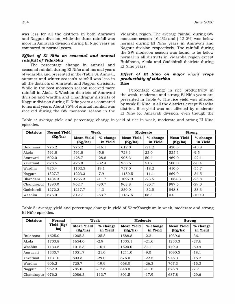
254 June 2020

was less for all the districts in both Amravati and Nagpur division, while the June rainfall was more in Amravati division during El Niño years as compared to normal years.

Effect of El Niño on seasonal and annual rainfall of Vidarbha

The percentage change in annual and seasonal rainfall during El Niño and normal years of vidarbha and presented in the (Table 3). Annual, summer and winter season’s rainfall was less in all the districts of Amravati and Nagpur divisions. While in the post monsoon season received more rainfall in Akola & Washim districts of Amravati division and Wardha and Chandrapur districts of Nagpur division during El Niño years as compared to normal years. About 75% of annual rainfall was received during the SW monsoon season in the

Vidarbha region. The average rainfall during SW monsoon season (-6.1%) and (-12.2%) was below normal during El Niño years in Amravati and Nagpur division respectively. The rainfall during the SW monsoon season was found to be below normal in all districts in Vidarbha region except Buldhana, Akola and Gadchiroli districts during El Niño years.

Effect of El Niño on major kharif crops productivity of vidarbhaRice

Percentage change in rice productivity in the weak, moderate and strong El Niño years are presented in Table 4. The rice yield was affected by weak El Niño in all the districts except Wardha district. Rice yield was not affected by moderate El Niño for Amravati division, even though the

Table 4: Average yield and percentage change in yield of rice in weak, moderate and strong El Niño episodes.

districts Normal Yield (Kg/ha)

Weak Moderate StrongMean Yield

(Kg/ha) % change in Yield

Mean Yield (Kg/ha)

% change in Yield

Mean Yield (Kg/ha)

% change in Yield

Buldhana 776.2 776.2 -16.1 612.0 -21.2 420.8 -45.8Akola 591.8 591.8 -5.8 728.1 23.0 535.3 -9.5Amravati 602.0 428.7 -28.8 905.3 50.4 469.0 -22.1Yavatmal 628.5 425.0 -32.4 953.5 51.7 500.0 -20.4Wardha 925.4 1102.5 19.1 757.0 -18.2 410.0 -55.7Nagpur 1327.7 1223.3 -7.9 1180.5 -11.1 869.0 -34.5Bhandara 1434.3 1266.3 -11.7 1097.9 -23.5 1064.3 -25.8Chandrapur 1390.0 962.7 -30.7 963.8 -30.7 987.5 -29.0Gadchiroli 1272.2 1217.7 -4.3 859.0 -32.5 848.8 -33.3Washim 676.0 312.7 -53.7 1137.5 68.3 0.0 -100.0

Table 5: Average yield and percentage change in yield of Kharif sorghum in weak, moderate and strong El Niño episodes.

districts Normal Yield (Kg/

ha)



Mean Yield (Kg/ha)

% change in Yield

Mean Yield (Kg/ha)

% change in Yield

Buldhana 1625.0 1205.3 -25.8 1588.8 -2.2 1039.0 -36.1Akola 1703.8 1654.0 -2.9 1335.1 -21.6 1233.3 -27.6Washim 1133.8 1015.3 -10.4 1520.0 34.1 449.0 -60.4Amravati 1330.7 1051.7 -21.0 1211.0 -9.0 1090.5 -18.1Yavatmal 1131.0 803.3 -29.0 876.0 -22.5 948.3 -16.2Wardha 906.2 725.7 -19.9 668.0 -26.3 767.3 -15.3Nagpur 952.3 785.0 -17.6 848.0 -11.0 878.8 -7.7Chandrapur 976.2 2086.3 113.7 801.5 -17.9 687.8 -29.6

rainfall was found to be below normal in all the districts. Strong El Niño has adversely affected the yield of rice in all the districts of Vidarbha. The less rainfall and high temperature noted during the El Niño year a caused reduction in the yield of rice.

Kharif sorghumPercentage change in the productivity of

Kharif sorghum in the weak, moderate and strong years is shown in Table 5. The Sorghum yield was below normal for all the districts in weak, moderate and strong El Niño episodes. But, the yield was better in weak El Niño episodes in Chandrapur district. During the strong El Niño episodes more reduction in yield was observed, whereas rainfall was also below normal as compared to weak and Table 6: Average yield and percentage change in yield of cotton in weak, moderate and strong El Niño episodes.




Mean Yield (Kg/ha)

% change in Yield

Mean Yield (Kg/ha)

% change in Yield

Buldhana 207.3 157.0 -24.3 153.8 -25.8 93.5 -54.9Akola 208.2 206.7 -0.7 158.8 -23.7 119.0 -42.8Washim 231.7 145.0 -37.4 187.0 -19.3 178.0 -23.2Amrawati 225.7 152.3 -32.5 150.8 -33.2 142.8 -36.7Yavatmal 194.6 154.7 -20.5 129.0 -33.7 107.0 -45.0Wardha 227.2 199.0 -12.4 174.5 -23.2 120.0 -47.2Nagpur 233.1 225.3 -3.3 173.8 -25.5 129.8 -44.3Chandrapur 218.0 224.3 2.9 149.0 -31.6 128.3 -41.2Gadchiroli 225.2 239.3 6.3 152.3 -32.4 155.7 -30.9

moderate El Niño.

CottonDistrict wise productivity of cotton in different

El Niño episodes in Vidarbha region is presented in Table 6. The cotton productivity was below normal for all the districts during weak Episodes except for Chandrapur and Gadchiroli districts. The percentage change in cotton productivity during moderate El Niño years was negative for all the districts. The percentage change in annual and SW monsoon rainfall was negative in a moderate El Niño episode. During Strong El Niño years also, cotton productivity was found to be below normal for the all districts in Vidarbha.

Table 7: Average yield and percentage change in yield of pigeon pea in weak, moderate and strong El Niño episodes.




Mean Yield (Kg/ha)

% change in Yield

Mean Yield (Kg/ha)

% change in Yield

Buldhana 730.4 562.7 -23.0 773.5 5.9 522.8 -28.4Akola 944.6 619.3 -34.4 838.6 -11.2 727.3 -23.0Washim 730.5 726.0 -0.6 1009.0 38.1 548.0 -25.0Amrawati 940.8 638.7 -32.1 866.3 -7.9 666.3 -29.2Yavatmal 932.1 619.7 -33.5 831.8 -10.8 649.0 -30.4Wardha 966.0 557.3 -42.3 801.5 -17.0 607.3 -37.1Nagpur 766.0 508.0 -33.7 603.5 -21.2 330.3 -56.9Bhandara 833.3 511.0 -38.7 668.2 -19.8 460.3 -44.8Chandrapur 730.8 421.3 -42.3 558.3 -23.6 516.5 -29.3Gadchiroli 835.7 312.0 -62.7 668.3 -20.0 457.0 -45.3Gondia 951.7 511.0 -46.3 791.0 -16.9 449.0 -52.8

Vol. 22, Special Issue KADAM et al. 255

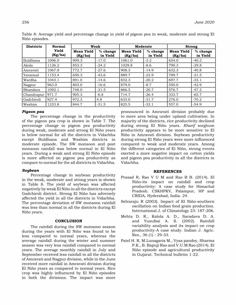
256 June 2020

Pigeon peaThe percentage change in the productivity

of the pigeon pea crop is shown in Table 7. The percentage change in pigeon pea productivity during weak, moderate and strong El Niño years is below normal for all the districts in Vidarbha except Buldhana and Washim districts in moderate episode. The SW monsoon and post monsoon rainfall was below normal in El Niño years. During a weak and strong El Niño episode is more affected on pigeon pea productivity as compare to normal for the all districts in Vidarbha.

SoybeanPercentage change in soybean productivity

in the weak, moderate and strong years is shown in Table 8. The yield of soybean was affected negatively by weak El Niño in all the districts except Gadchiroli district. Strong El Niño has adversely affected the yield in all the districts in Vidarbha. The percentage deviation of SW monsoon rainfall was less than normal in all the districts during El Niño years.

CoNCLuSIoNThe rainfall during the SW monsoon season

during the years with El Niño was found to be less compared to normal years, whereas the average rainfall during the winter and summer season was very less rainfall compared to normal years. The average monthly rainfall in July and September received less rainfall in all the districts of Amravati and Nagpur division, while in the June received more rainfall in Amravati division during El Niño years as compared to normal years. Rice crop was highly influenced by El Niño episodes in both the divisions. The impact was more

pronounced in Amravati division probably due to more area being under upland cultivation. In majority of the districts, rice productivity declined during strong El Niño years. Kharif sorghum productivity appears to be more sensitive to El Niño in Amravati division. Soybean productivity during strong El Niño years were more influenced compared to weak and moderate years. Among the different categories of El Niño, strong events exerted a more negative impact on cotton yields and pigeon pea productivity in all the districts in Vidarbha.

reFereNCeS Prasad R, Rao V U M and Rao B B. (2014). El

Niño-its impact on rainfall and crop productivity: A case study for Himachal Pradesh. CSKHPKV, Palampur, HP and CRIDA, Hyderabad, India. 24.

Selvaraju R (2003). Impact of El Niño-southern oscillation on Indian food grain production. International J. of Climatology 23: 187-206.

Mehta D. R., Kalola A. D., Saradava D. A. and Yusufzai A. S. (2002). Rainfall variability analysis and its impact on crop productivity-A case study. Indian J. Agric. Res., 36 (1) : 29-33.

Patel H. R, M.Lunagaria M., Vyas pandey, Sharma P.K., B. Bapuji Rao and V.U.M Rao (2014). El Niño episode and agricultural productivity in Gujarat. Technical bulletin 1-22.

Table 8: Average yield and percentage change in yield of pigeon pea in weak, moderate and strong El Niño episodes.

districts Normal Yield

(Kg/ha)



Mean Yield (Kg/ha)

% change in Yield

Mean Yield (Kg/ha)

% change in Yield

Buldhana 1096.0 909.3 -17.0 1061.0 -3.2 654.0 -40.3Akola 1126.2 853.3 -24.2 1029.8 -8.6 790.3 -29.8Amravati 1067.8 772.7 -27.6 908.3 -14.9 632.3 -40.8Yavatmal 1153.4 650.3 -43.6 889.7 -22.9 789.7 -31.5Wardha 1043.1 891.0 -14.6 832.3 -20.2 697.7 -33.1Nagpur 963.0 803.0 -16.6 879.0 -8.7 550.0 -42.9Bhandara 1092.1 748.0 -31.5 866.5 -20.7 576.7 -47.2Chandrapur 971.7 905.3 -6.8 714.7 -26.4 333.7 -65.7Gadchiroli 927.4 972.3 4.8 633.0 -31.7 276.0 -70.2Washim 1233.8 844.7 -31.5 825.5 -33.1 557.0 -54.9

evaluation of heat stress level for effective management of dairy cattle in Jorhat district of assam

ParIShMIta daS, r. L. deKa aNd r. huSSaINDepartment of Agrometeorology

Assam Agricultural University, Jorhat-785013, Assam, India

aBStraCtTemperature-humidity index (THI), a calculated index that incorporates the effects of temperature with relative humidity, was calculated to determine the exposure of dairy cattle to different levels of heat stress in Jorhat district of Assam utilizing daily temperature and relative humidity data during 2004-2018. Results showed that, annually, dairy cattle remained completely stress free (THI<72) for 189 days while they were exposed to ‘mild stress’ and ‘moderate stress’ in 132 and 44 days, respectively during morning. However, more number of days was under moderate (164 days) and mild (131 days) stress during afternoon hours compared to no stress days (66). Analysis also revealed that the “moderate stress” days were observed during all the seasons except in winter, being prominently higher towards the afternoon (109 days) during monsoon. To alleviate mild and moderate stress on dairy cattle, the planning and construction of cattle shed design is of utmost importance particularly for exotic breeds.

Keywords: THI, heat stress, dairy cattle, Assam

INtroduCtIoN

Livestock, which contributes to diverse agri-food systems globally, forms an integral part of most of the agriculture dependent families of Assam by helping them to generate supplementary income (Borah and Halim, 2014). Sustainability in livestock production has been largely affected by rapid urbanization and globalization (FAO, 2018) along with the increasing global temperature. Being homoeothermic by nature, dairy cattle are more susceptible to heat stress (HS) compared to other ruminants, as they generate more metabolic heat (Das et al., 2016).Under the influence of high temperature and humid climates, dairy cattle are exposed to HS, a situation in which the effective temperature of the environment is higher than the animal’s thermo-neutral (comfort) zone (Armstrong, 1994) leading to a imbalance between metabolic heat production and its dissipation to the surroundings. The severity of HS on dairy cattle will increase as global warming progresses not only in tropics but also in the northern latitudes. HS has negative effects on the health and biological functioning of dairy cattle through depressed milk production and reduced reproductive performance (Polsky and von Keyserlingk, 2017), especially in lactating cows. Other obvious signs of HS includethe incidence of diseases, decrease in feed intake, metabolism, body weight (Gantner et al., 2011), lethargic behaviour, profuse

sweating, open mouth panting, etc. Heat stroke is common in severe cases when complicated with other stresses like illness and calving (Pennington and Devender, 2011). Besides the environmental factors, HS severity also depends on cattle breed, developmental stage, coat colour, level of milk production and dry matter intake prior to the heat stress, housing design, etc. (Atrian and Shahryar, 2012).

In Assam, the total livestock population is 1, 96, 15, 490 (3.25% of thecountry’s total population) of which cattle holds the highest position with a population of 1, 03, 07, 700 including both indigenous (96.16%) and exotic (3.84%) breeds (DAH, 2012). Indigenous breeds include mostly non-descript local breeds with a small population of Sahiwal cross and Red Sindhi whereas Jersey cross and Holstein Friesian cross are the exotic breeds. The present study was undertaken to ascertain the exposure of dairy cattle to different levels of heat stress in humid and per-humid climatic conditions of Jorhat which will help in formulating different management strategies to alleviate the negative impacts of HS, if any and timely dissemination of effective agroadvisories to the farming community.


Jorhat district, situated in the eastern part


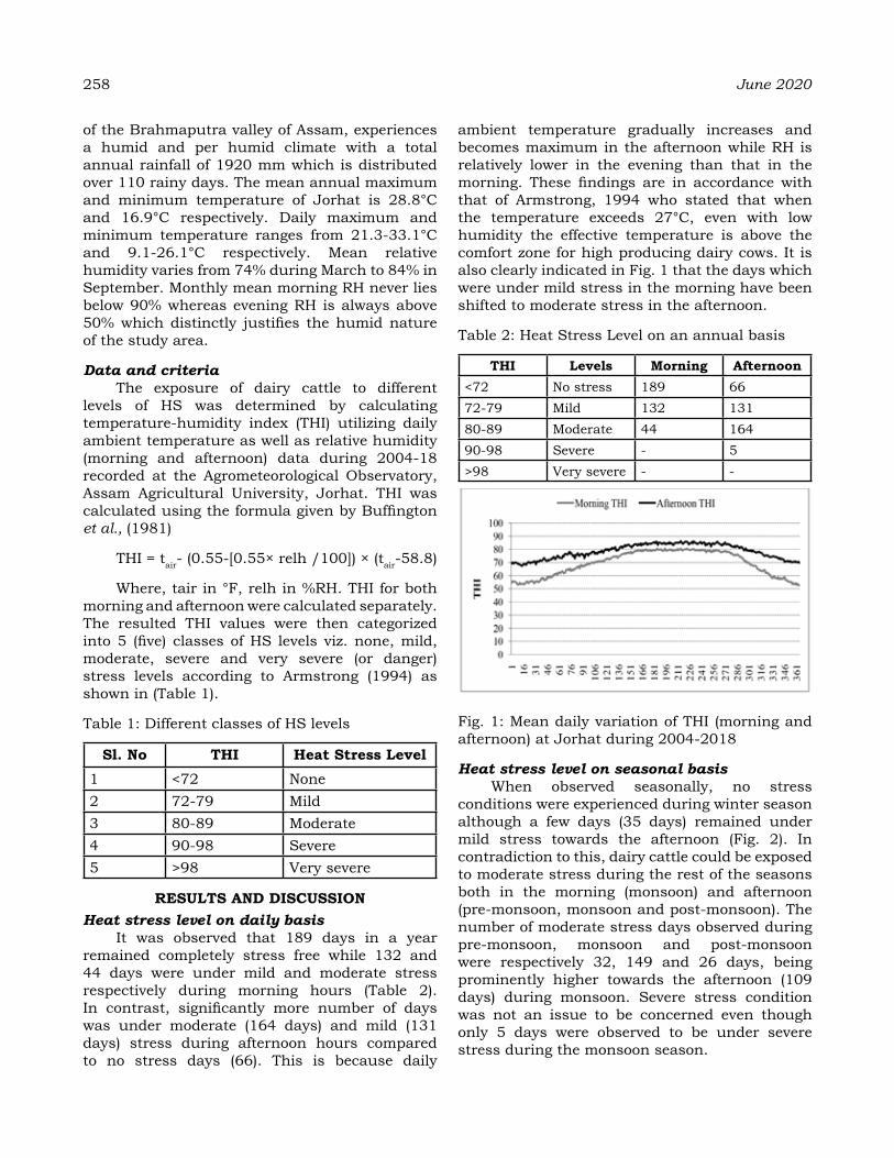
258 June 2020

of the Brahmaputra valley of Assam, experiences a humid and per humid climate with a total annual rainfall of 1920 mm which is distributed over 110 rainy days. The mean annual maximum and minimum temperature of Jorhat is 28.8°C and 16.9°C respectively. Daily maximum and minimum temperature ranges from 21.3-33.1°C and 9.1-26.1°C respectively. Mean relative humidity varies from 74% during March to 84% in September. Monthly mean morning RH never lies below 90% whereas evening RH is always above 50% which distinctly justifies the humid nature of the study area.

Data and criteriaThe exposure of dairy cattle to different

levels of HS was determined by calculating temperature-humidity index (THI) utilizing daily ambient temperature as well as relative humidity (morning and afternoon) data during 2004-18 recorded at the Agrometeorological Observatory, Assam Agricultural University, Jorhat. THI was calculated using the formula given by Buffington et al., (1981)

THI = tair- (0.55-[0.55× relh /100]) × (tair-58.8)

Where, tair in °F, relh in %RH. THI for both morning and afternoon were calculated separately. The resulted THI values were then categorized into 5 (five) classes of HS levels viz. none, mild, moderate, severe and very severe (or danger) stress levels according to Armstrong (1994) as shown in (Table 1).

Table 1: Different classes of HS levels

Sl. No thI heat Stress Level1 <72 None2 72-79 Mild3 80-89 Moderate4 90-98 Severe5 >98 Very severe

reSuLtS aNd dISCuSSIoNHeat stress level on daily basis

It was observed that 189 days in a year remained completely stress free while 132 and 44 days were under mild and moderate stress respectively during morning hours (Table 2). In contrast, significantly more number of days was under moderate (164 days) and mild (131 days) stress during afternoon hours compared to no stress days (66). This is because daily

ambient temperature gradually increases and becomes maximum in the afternoon while RH is relatively lower in the evening than that in the morning. These findings are in accordance with that of Armstrong, 1994 who stated that when the temperature exceeds 27°C, even with low humidity the effective temperature is above the comfort zone for high producing dairy cows. It is also clearly indicated in Fig. 1 that the days which were under mild stress in the morning have been shifted to moderate stress in the afternoon.

Table 2: Heat Stress Level on an annual basis

thI Levels Morning afternoon<72 No stress 189 6672-79 Mild 132 13180-89 Moderate 44 16490-98 Severe - 5>98 Very severe - -

Fig. 1: Mean daily variation of THI (morning and afternoon) at Jorhat during 2004-2018

Heat stress level on seasonal basisWhen observed seasonally, no stress

conditions were experienced during winter season although a few days (35 days) remained under mild stress towards the afternoon (Fig. 2). In contradiction to this, dairy cattle could be exposed to moderate stress during the rest of the seasons both in the morning (monsoon) and afternoon (pre-monsoon, monsoon and post-monsoon). The number of moderate stress days observed during pre-monsoon, monsoon and post-monsoon were respectively 32, 149 and 26 days, being prominently higher towards the afternoon (109 days) during monsoon. Severe stress condition was not an issue to be concerned even though only 5 days were observed to be under severe stress during the monsoon season.

Fig. 2: Seasonal variation in heat stress levels (I-Morning; II-Afternoon) at Jorhat during 2004-2018

Monthly distribution of HS daysIt was observed that mild stress began to

develop in the morning hours from April which remained till October (Fig. 3). In contrast, mild stress was observed in all the months during afternoon hours with varying magnitudes. In the afternoon hours, all the months except December and January experienced moderate stress, being distinctively highest in the month of July (29 days). Severe stress days were distributed in May, June, July, August and September during afternoon hours.

Fig. 3: Monthly variation in heat stress levels during the morning (a) and afternoon (b) hours at Jorhat during 2004-2018

Heat Stress Management StrategiesThe most convenient and natural means

of abating HS in dairy cattle is their inherent capability to thermo regulate (Polsky and von Keyserlingk, 2017). However, different artificial techniques have been developed in due course of time to encounter numerous challenges of HS. One of the most important components which need to be taken care of for effective management of dairy cattle is the dairy housing system. The cattle shed must be designed and oriented to reduce the heat load as HS could be more detrimental compared to cold stress (Belsare and Pandey, 2008). The cattle shed must be provided with gunny bag curtains in order to prevent the penetration of direct sunlight during summer. This would also prevent the cold winds blowing into the shed during high windy days. The results indicated that HS was at its peak level during the monsoon season. Use of water as a cooling agent either directly on the animal body, spraying water on the floor and roof of shelter (Belsare and Pandey, 2008) or sprinkling water on the gunny curtains can effectively reduce the heat load on dairy cattle during monsoon and summer as well. Besides, provision of proper cross ventilation, planting trees near the cattle shed, installation of fans inside the shed and washing the cattle with cold water can prove to be effective interventions to improve the coping abilities of heat-stressed cattle during the summer months.

It has been reported that native Indian cattle or the local breeds are more beneficial as draught animals while crossbred exotic cattle, which contains more than 75% of exotic blood, serve as a better options in case of higher milk production (Kohli et al., 2014). But, HS has a negative impact on the milk yield of exotic cows due to insufficient secretion of reproductive hormones (Bun et al., 2017). Therefore, to reduce the negative impact of HS to a certain extent, exotic breeds may be allowed for controlled grazing during early morning. Moreover, as the moderate and mild stress were more prominent during the afternoon hours, it is desirable that dairy cattle graze in the open fields during morning and return to their shed towards afternoon.

CoNCLuSIoNDifferent HS levels were determined by

calculating THI on daily, monthly and seasonal basis utilizing daily dry bulb temperature and relative humidity data at Jorhat. It was observed

Vol. 22, Special Issue DAS et al. 259

260 June 2020

that high ambient air temperature (>75°F) accompanied by high relative humidity (>90%) had negative effects on the comfort level of dairy cattle, owing to the humid climate of the study area. Heat stress days (mild and moderate) persisted only for 175 days during morning while more than 300 days remained under stress during afternoon hours. Quantification of heat stress levels will help in formulating effective weather-based advisories which would not only improve the performance of dairy cattle but also sustain the livelihood of the rural inhabitants.

reFereNCeSArmstrong, D. V. (1994). Heat Stress Interaction

with Shade and Cooling.J. Dairy Sci., 77:2044-2050.

Atrian, P. and Shahryar, H. A. (2012).Heat Stress in Dairy Cows (A Review).Research in Zoology, 2 (4) : 31-37.

Belsare, V.P. and Pandey, V. (2008).Management of heat stress in dairy cattle and buffaloes for optimum productivity. J. Agrometeorol., 365-368.

Borah, M. and Halim, R. A. (2014). Dynamics of Livestock and Poultry Sector in Assam: A Critical Analysis. Econ. Affairs, 59: 773-782.

Buffington, D. E., Collazo-Arocho, A., Canton, G. H., Pitt, D., Thatcher, W. W. and Collier, R. J. (1981).Black globe-humidity index (BGHI) as comfort equation for dairy cows. Trans ASAE, 24 (3) : 0711-0714.

Bun, C., Watanabe, Y., Uenoyama, Y., Inoue, N., Ieda, N., Ieda, N., Matsuda, F., Tsukamura, H., Kuwahara, M., Maeda, K., Ohkura, S.

and Pheng, V. (2017). Evaluation of heat stress response in crossbred dairy cows under tropical climate by analysis of heart rate variability. J. Vet. Med. Sci., 80 (1) : 181–185.

DAH (2012).Department of Animal Husbandry, 19th livestock census, Ministry of Agriculture, Dairying and Fisheries, 2012.

Das, R., Sailo, L., Verma, N., Bharti, P., Saikia, J., Imtiwati and Kumar, R. (2016).Impact of heat stress on health and performance of dairy animals: A review. Vet World., 9 (3) : 260–268.

FAO, FAOSTATS (2018). Food and Agriculture Organization of the United Nations, Rome, http://faostat.fao.org/default.aspx.2018.

Gantner, V., Mijić1, P., Kuterovac, K., Solić, D. and Gantner, R. (2011). Temperature-humidity index values and their significance on the daily production of dairy cattle. Daily production of dairy cattle, Mljekarstvo, 61 (1) : 56-63.

Kohli, S., Atheya, U. K. and Thapliyal, A. (2014).Assessment of optimum thermal humidity index for crossbred dairy cows in Dehradun district, Uttarakhand, India. Vet. World, 7 (11) : 916-921.

Pennington, J. A. and Devender, K. V. (2011). Heat stress in dairy cattle. University of Arkansas Cooperative Extension Service Printing Services.2011; FSA 3040- PD-1- 06RV. Or web site at: http://www.udex. Edu/.

Polsky, L. and Keyserlingk, M. A. G. (2017). Invited review: Effects of heat stress on dairy cattle welfare. J. Dairy Sci., 100:8645–8657.

effect of rainfall, anthropogenic activities and geomorphology on groundwater Levelof hisar district, haryana

dharMeNdra SINgh1*, NIMISh NaraYaN gautaM1, darShaNa duhaN2, SaNdeeP arYa2, rS hooda1, vS arYa1,

1Haryana Space Applications Centre, CCS HAU Campus, Hisar 2Chaudhary Charan Singh Haryana Agricultural University, Hisar

*Coresponding author: [email protected]

aBStraCtGroundwater is an important natural resource for human survival on earth and an integral part of hydrological cycle. Its availability largely depends on rainfall, anthropogenic activities and recharge conditions. Thus the current study was done to evaluate the impact of rainfall on groundwater resources along with the assessment of impacts of recharge condition and anthropogenic activities over Hisar district of Haryana. India Meteorological Department (IMD) rainfall product with spatial resolution of 0.25°×0.25° was used for the assessment of rainfall during the period 1996 to 2016. India Water Resource Information System (WRIS) based groundwater resource information were taken for the analyses of groundwater level of post monsoon period. Geomorphology data were take from Haryana Space Application centre (HARSAC). First the groundwater level were interpolated using kriging interpolation method in ArcGIS software and then change analysis was done both inside and out side boundary of anthopogenic activity implementation sites. Overall decrease in groundwater since 1996 to 2016 with positive impact of rainfall was observed. However, it was found to be positively affected by the interaction of all the factors including rainfall, anthropogenic activities and recharge conditions over Hisar district.

Keywords: Groundwater level, Rainfall, interpolation, Geomorphology, Hisar

INtroduCtIoN

Groundwater is an important natural resource for human survival on earth and an integral part of hydrological cycle. It contribute a total of 1/5 part of the current world water requirement. Some of the countries in the world like Denmark, Malta, Saudi Arabia, etc. are totally depends on groundwater. Most of the European countries fulfill their water needs by exploiting 70% of groundwater (Zektser and Everett, 2004). The condition is similar in India and about 50% of the water requirement is fulfilled by groundwater. According to a statistic of Central Water Commission (CWB) India, a total of 433 billion cubic meter/year water is available as groundwater (Suhag, 2016).

Ground water availability largely depends on rainfall, anthropogenic activities, barometric pressure, earth tide and recharge conditions. Rainfall alone contributes a total of 68% in groundwater resource of India (Suhag, 2016). Thus a significant impact of rainfall on groundwater level is found in several studies. Tirogo et al., (2016) reported the effect of decreased rainfall condition and increased evapotranspiration on groundwater level at catchment area scale. They found that the groundwater shows delayed

response with rainfall which may varies from 1 to 4 months on seasonal scale and one year on inter-annual variation time scale. It is highly dependent on characteristics of local aquifer condition. They further reported that the groundwater level is dependent on various parameters including climatic factor, vegetation, Land Use Land Cover, soil types, and geology. The change in climatic factors affects atmospheric water vapor content, precipitation and evapotranspiration pattern, soil moisture content and temperature, surface and stream runoff, ice melting among others which further affects the global subsurface hydrologic cycle including groundwater (Bates et al., 2008; Van Dijck et al., 2006; Green et al., 2011). Vegetation type and its root system determine the groundwater scenario. Vegetation with broad leaves and deep rooted system contributes more in discharge but maintains deep water table (Alaghmand et al., 2014). Similarly conversion of grasslands to scrubland to crop land (Land use Land cover) change the system from discharge to the recharge by reducing evapotranspiration rates (Scanlon et al., 2005). The percolation of water inside the ground for recharge is dependents on percolation factor which in turn depends on hydraulic conductivity a specific


262 June 2020

characteristic of soil type (da Costa et al., 2019). Similarly geology and geomorphology affects the recharge conditions as reported by Rajaveni et al., (2017) and provided highest weight age in the groundwater recharge. These parameters (climatic factor, vegetation, Land Use Land Cover, soil types, and geology/geomorphology) together are used for identifying groundwater recharge zones using multi-criteria decision system (da Costa et al., 2019). Detail studies have been carried out for deep understanding of various factors involved in groundwater recharge.

Lorenzo-Lacruz et al., (2017) analyzed the effect of rainfall variability on groundwater level using Standardized Precipitation Index (SPI) and Standardized Groundwater Index (SGI) over Mediterranean regions. Further it was detected that the recharge of various aquifers is intimately dependent on meteorological conditions and highly correlated with peak precipitation. They found that the recharge is more in plain areas as compared to hilly regions.

Jasechko and Taylor (2015) studied the positive impact of intensive rainfall on groundwater based on isotope method. The found that the groundwater storage has increase in the tropics due to rainfall variability however, the appropriate science behind this was not explained. Thus studies from across the world showed the positive impact of rainfall on groundwater level.

Few studies from India relating rainfall with groundwater recharge showed similar results. Asoka et al., (2018) identified the significant impact of precipitation of groundwater. They reported a decline rate of 2 cm yr−1 in groundwater over northern part of India. The main driving force identified for the groundwater storage variability was changes in long-term monsoon precipitation Chinnasamy and Agoramoorthy (2015) reported that the exploitation rate of groundwater is 8% higher than the recharge of groundwater in Tamil Nadu region. Thakkar et al., (2017) evaluated the impact of watershed management practices on LULC dynamic using Land sat Enhanced Thematic mapper (ETM+) and Linear Imaging Self Scanning (LISS-III) data over a semi-arid watershed in Gujarat and concluded that the area of agriculture and water has been increased due to enhanced water availability resulted from watershed management practices. Bhanja et al., (2017) reported increase in groundwater storage in southern and eastern part of India due to water

management policies. They used both satellite and ground based observation to assess the changes in groundwater storage during 1996 to 2014.

Despite these studies it was also found that the anthropogenic activities are important governing factor for groundwater storage. The studies done at watershed level have made it more clear (Shanwad et al., 2012; Singh et al., 2013; Sinha et al., 2017; Thakkar et al., 2017).Singh et al., (2013) reported the positive impacts of Integrated Watershed Development activities on forest area increase using Landsat data during 1990 to 2011 over a watershed region of Seoni district India. They further used Soil brightness Index (SBI) and NDVI to assess the change in the condition of the forest. They concluded that the forest condition was improved and agricultural area was increased possibly due to increase in groundwater however, they have not analysed the groundwater scenario over the study region. The impacts and efficiency of Punjab sub-soil water Act 2009 was assessed by Singh et al., (2016) using passive radiometer based measurement from AMSR-E and SPOT NDVI data. They concluded that the Act is effective in the rice belt. The increase in groundwater has also been reported in the same region by Bhanja et al., (2017) due to various water conservation policies such as the Punjab sub-soil water Act 2009, Integrated Watershed Management Program (IWMP).

Managing groundwater and surface water through watershed approach is another best and effective technique which is most utilized technique for poverty mitigation, food safety, society welfare and socio-economic conditions, natural resource management, ecological benefits, water conservation, etc. among others (Shanwad et al., 2012). IWMP, an important anthropogenic activity was implemented across Haryana state in a participatory and scientific way with the objective to restore ecological balance for recharging of the groundwater. These programs enables multi-cropping and the introduction of various agro-based activities, which supports sustainable livelihoods to the people residing in the watershed area along with increase in groundwater level (Shanwad et al., 2012; Singh et al., 2013; Sinha et al., 2017).

The groundwater level is also being influenced by geomorphology of a given area. The determination of groundwater “zonation” is generally based on interactive processing among geomorphology,

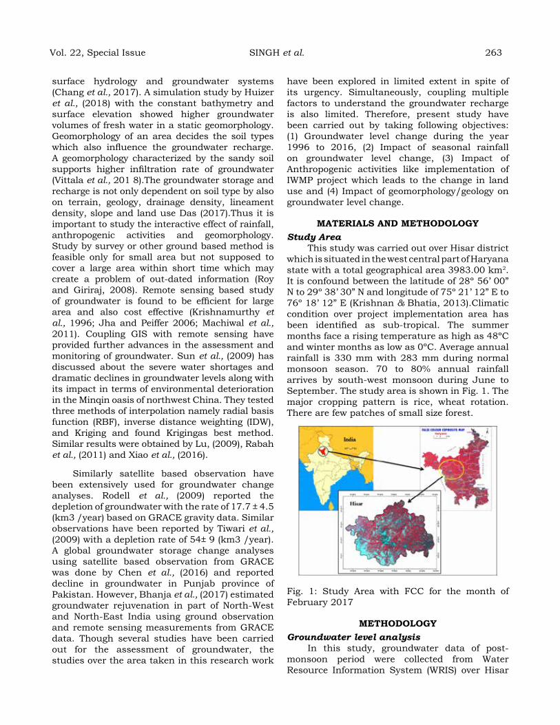
surface hydrology and groundwater systems (Chang et al., 2017). A simulation study by Huizer et al., (2018) with the constant bathymetry and surface elevation showed higher groundwater volumes of fresh water in a static geomorphology. Geomorphology of an area decides the soil types which also influence the groundwater recharge. A geomorphology characterized by the sandy soil supports higher infiltration rate of groundwater (Vittala et al., 201 8).The groundwater storage and recharge is not only dependent on soil type by also on terrain, geology, drainage density, lineament density, slope and land use Das (2017).Thus it is important to study the interactive effect of rainfall, anthropogenic activities and geomorphology. Study by survey or other ground based method is feasible only for small area but not supposed to cover a large area within short time which may create a problem of out-dated information (Roy and Giriraj, 2008). Remote sensing based study of groundwater is found to be efficient for large area and also cost effective (Krishnamurthy et al., 1996; Jha and Peiffer 2006; Machiwal et al., 2011). Coupling GIS with remote sensing have provided further advances in the assessment and monitoring of groundwater. Sun et al., (2009) has discussed about the severe water shortages and dramatic declines in groundwater levels along with its impact in terms of environmental deterioration in the Minqin oasis of northwest China. They tested three methods of interpolation namely radial basis function (RBF), inverse distance weighting (IDW), and Kriging and found Krigingas best method. Similar results were obtained by Lu, (2009), Rabah et al., (2011) and Xiao et al., (2016).

Similarly satellite based observation have been extensively used for groundwater change analyses. Rodell et al., (2009) reported the depletion of groundwater with the rate of 17.7 ± 4.5 (km3 /year) based on GRACE gravity data. Similar observations have been reported by Tiwari et al., (2009) with a depletion rate of 54± 9 (km3 /year). A global groundwater storage change analyses using satellite based observation from GRACE was done by Chen et al., (2016) and reported decline in groundwater in Punjab province of Pakistan. However, Bhanja et al., (2017) estimated groundwater rejuvenation in part of North-West and North-East India using ground observation and remote sensing measurements from GRACE data. Though several studies have been carried out for the assessment of groundwater, the studies over the area taken in this research work

have been explored in limited extent in spite of its urgency. Simultaneously, coupling multiple factors to understand the groundwater recharge is also limited. Therefore, present study have been carried out by taking following objectives: (1) Groundwater level change during the year 1996 to 2016, (2) Impact of seasonal rainfall on groundwater level change, (3) Impact of Anthropogenic activities like implementation of IWMP project which leads to the change in land use and (4) Impact of geomorphology/geology on groundwater level change.

MaterIaLS aNd MethodoLogYStudy Area

This study was carried out over Hisar district which is situated in the west central part of Haryana state with a total geographical area 3983.00 km2. It is confound between the latitude of 28º 56’ 00” N to 29º 38’ 30” N and longitude of 75º 21’ 12” E to 76º 18’ 12” E (Krishnan & Bhatia, 2013).Climatic condition over project implementation area has been identified as sub-tropical. The summer months face a rising temperature as high as 48ºC and winter months as low as 0ºC. Average annual rainfall is 330 mm with 283 mm during normal monsoon season. 70 to 80% annual rainfall arrives by south-west monsoon during June to September. The study area is shown in Fig. 1. The major cropping pattern is rice, wheat rotation. There are few patches of small size forest.

Fig. 1: Study Area with FCC for the month of February 2017

MethodoLogYGroundwater level analysis

In this study, groundwater data of post-monsoon period were collected from Water Resource Information System (WRIS) over Hisar


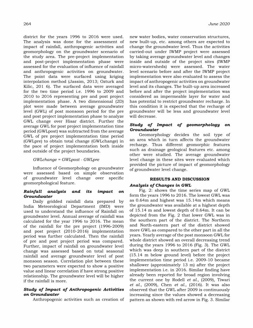
264 June 2020

district for the years 1996 to 2016 were used. The analysis was done for the assessment of impact of rainfall, anthropogenic activities and geomorphology on the groundwater scenario of the study area. The pre-project implementation and post-project implementation phase were assessed for the evaluation of influence of rainfall and anthropogenic activities on groundwater. The point data were surfaced using kriging interpolation method (Jassim, 2013; Ozturk and Kilic, 201 6). The surfaced data were averaged for the two time period i.e. 1996 to 2009 and 2010 to 2016 representing pre and post project implementation phase. A two dimensional (2D) plot were made between average groundwater level (GWL) of post monsoon period for the pre and post project implementation phase to analyze GWL change over Hisar district. Further the average GWL for post project implementation time period (GWLpost) was subtracted from the average GWL of pre project implementation time period (GWLpre) to obtain total change (GWLchange) in the pace of project implementation both inside and outside of the project boundaries.

GWLchange = GWLpost - GWLpre

Influence of Geomorphology on groundwater were assessed based on simple observation of groundwater level change over specific geomorphological feature.

Rainfall analysis and its impact on Groundwater

Daily gridded rainfall data prepared by India Meteorological Department (IMD) were used to understand the influence of Rainfall on groundwater level. Annual average of rainfall was calculated for the year 1996 to 2016. The mean of the rainfall for the pre project (1996-2009) and post project (2010-2016) implementation period was further calculated. Then the rainfall of pre and post project period was compared. Further, impact of rainfall on groundwater level change was assessed based on total seasonal rainfall and average groundwater level of post monsoon season. Correlation plot between these two parameters were expected to show a positive value and linear correlation if have strong positive relationship. The groundwater level will be higher if the rainfall is more.

Study of Impact of Anthropogenic Activities on Groundwater

Anthropogenic activities such as creation of

new water bodies, water conservation structures, new built-up, etc. among others are expected to change the groundwater level. Thus the activities carried-out under IWMP project were assessed by taking average groundwater level and changes inside and outside of the project sites (IWMP micro-watersheds) were assessed. The water level scenario before and after the IWMP project implementation were also evaluated to assess the impact of anthropogenic activities on groundwater level and its changes. The built-up area increased before and after the project implementation was considered as impermeable layer for water and has potential to restrict groundwater recharge. In this condition it is expected that the recharge of groundwater will be less and groundwater level will decrease.

Study of Impact of geomorphology on Groundwater

Geomorphology decides the soil type of an area which in turn affects the groundwater recharge. Thus different geomorphic features such as drainage geological features etc. among other were studied. The average groundwater level change in these sites were evaluated which provided the picture of impact of geomorphology of groundwater level change.

reSuLtS aNd dISCuSSIoNAnalysis of Changes in GWL

Fig. 2: shows the time series map of GWL form the years 1996 to 2016. The lowest GWL was as 0.64m and highest was 15.14m which means the groundwater was available at a highest depth of 15.14 m and lowest depth of 0.64m. It can be depicted from the Fig. 2 that lower GWL was in the southern part of the district. The Northern and North-eastern part of the district showed more GWL as compared to the other part in all the years. Yearly average of the post monsoon GWL for whole district showed an overall decreasing trend during the years 1996 to 2016 (Fig. 3). The GWL which was deep in southern part of the district (15.14 m below ground level) before the project implementation time period i.e. 2009-10 became shallower (approximately 13 m) after the project implementation i.e. in 2016. Similar finding have already been reported for broad region involving the current one by Rodell et al., (2009), Tiwari et al., (2009), Chen et al., (2016). It was also observed that the GWL after 2009 is continuously increasing since the values showed a decreasing pattern as shown with red arrow in Fig. 3. Similar

findings have been reported by Bhanja et al., (2017).

Fig. 2: Variations in GWL of the Hisar district for the post monsoon period during 1996 to 2016

Fig. 3: GWL of the years 1996 to 2016 (red arrow is showing increase in GWL after the year 2009)

Impact of rainfall on groundwater level change

The annual and seasonal rainfall during 1996 to 2016 was estimated from daily data of IMD. Annual average rainfall is represented as column graph in Fig. 4. Further annual rainfall for the pre project period and post project period were made and compared. It was observed that the rainfall is not varying much and similar amount of rainfall were received both in pre (328.70 mm) and post (319.25 mm) project implementation period (Table 2). Highest annual rainfall (516.44 mm) was obtained during the year 2005 and lowest (145.94 mm) during 2002. The seasonal sum of rainfall was calculated to assess the impact of rainfall on groundwater level recharge. Yearly seasonal rainfall and groundwater level were plotted together which proves the positive impact of rainfall on groundwater level recharge (Fig. 5).

Fig. 4: Annual rainfall variation of Hisar district during the year 1996 to 2016

Fig. 5: Relation between rainfall and ground water level

Seasonal rainfall was taken because we were trying to see the influence of rainfall on the groundwater level of post monsoon period. By

Table 2: Annual rainfall in Hisar District during 1996 to 2016

Years 1996 1997 1998 1999 2000 2001 2002 2003 2004 2005 2006Rainfall (mm) 359 450 351 327 213 205 145 188 208 516 341Years 2007 2008 2009 2010 2011 2012 2013 2014 2015 2016Rainfall (mm) 446 486 362 282 290 273 454 265 377 291


266 June 2020

seeing the relationship between seasonal rainfall and groundwater level it was observed that the r2 value is very less (i.e. 0.11 only) however, the positive trend showed that the rainfall is influencing groundwater level recharge of Hisar district.This simply means if the rainfall amount received is higher in a season of any year the post monsoonal groundwater level will be high for that year.The less r2 showed that the influence is not asstrong as expected and reported by various researchers like Scanlon et al., (2005), Lorenzo-Lacruz et al., (2017), ), Singh et al., (2017). This is because the variation in groundwater level change is also governed by to pattern of groundwater extraction which is varying across the district. Northern and North eastern part is having high pressure of anthropogenic water extraction while the southern and south western part is having less pressure of water extraction.

Evaluation of Impact of Anthropogenic activities on Groundwater level change

It was expected that IWMP activities related to water conservation either increase the groundwater of project site or the rate of reduction of groundwater will be less from outside of the project sites. The analysis of groundwater from the year 1997 to 2016 was done. The representation of GWL is such that the higher values indicates less GWL and lower values of GWL shows high level of groundwater. The results are described under following heads.

GWL change due to IWMP activitiesSince the IWMP project was implemented

during 2010-2011 over seven sites of Hisar district, its impact on groundwater was analyzed mainly based on average GWL before and after project implementation. Finally GWL change within project boundary and outside of it was analyzed to check our perception that the rate of change of GWL within IWMP project boundary would be less as compared to changes in GWL of outside the project boundary. Time period 1996 to 2009 was taken for pre-project change assessment and 2010 to 2016 for post project change assessment.

Pre-project GWL (1996 to 2009) Average groundwater level of Hisar district for

post monsoon period (Rabi season) during 1996 to 2009 was analyzed. Average Groundwater level was varying from 2.1 to 13.3m (Fig. 6). The highest level of groundwater was found in the eastern part of the Hisar district and varies from 2.1 to 6.3m. Central and northwest parts were having

medium GWL ranging from 6.4 to 9.1 m. Lowest GWL i.e. highest depth of groundwater from the earth surface was in south and southwestern part of Hisar district and varying from 9.1 to 12 m.

Fig. 6: Average groundwater level of Hisar district for the post-monsoon period (1996 to 2009)

Post-Project GWL (2010 to 2016) GWL of Hisar district for the post monsoon

period (Rabiseason) was averaged for assessing changes after project implementation i.e. during 2010 to 2016 (Fig. 7). The highest GWL 2.1m was still in the eastern part of Hisar district but the coverage of high water level portion had decreased drastically. This decrease was due to utilization of groundwater for irrigation and drinking purposes. Central and northern parts of the district were having medium GWL ranging from 6.4 to 9.1 m. These parts showed increase of in coverage area as compared to area of same groundwater level range before project implementation. This decrease in groundwater level is further due to population increase, using groundwater for irrigation and drinking. Lowest GWL was 12 m in southwestern part of Hisar district. This area was showing the highest depth of GWL with maximum area under 9.2 to 11 m range, which showed that the groundwater in this area had lost with lower rate.

Fig. 7: Average groundwater level of Hisar district for the post-monsoon period (2010 to 2016)

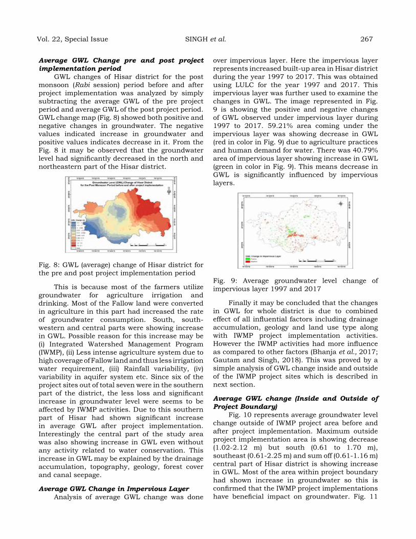
Average GWL Change pre and post project implementation period

GWL changes of Hisar district for the post monsoon (Rabi session) period before and after project implementation was analyzed by simply subtracting the average GWL of the pre project period and average GWL of the post project period. GWL change map (Fig. 8) showed both positive and negative changes in groundwater. The negative values indicated increase in groundwater and positive values indicates decrease in it. From the Fig. 8 it may be observed that the groundwater level had significantly decreased in the north and northeastern part of the Hisar district.

Fig. 8: GWL (average) change of Hisar district for the pre and post project implementation period

This is because most of the farmers utilize groundwater for agriculture irrigation and drinking. Most of the Fallow land were converted in agriculture in this part had increased the rate of groundwater consumption. South, south-western and central parts were showing increase in GWL. Possible reason for this increase may be (i) Integrated Watershed Management Program (IWMP), (ii) Less intense agriculture system due to high coverage of Fallow land and thus less irrigation water requirement, (iii) Rainfall variability, (iv) variability in aquifer system etc. Since six of the project sites out of total seven were in the southern part of the district, the less loss and significant increase in groundwater level were seems to be affected by IWMP activities. Due to this southern part of Hisar had shown significant increase in average GWL after project implementation. Interestingly the central part of the study area was also showing increase in GWL even without any activity related to water conservation. This increase in GWL may be explained by the drainage accumulation, topography, geology, forest cover and canal seepage.

Average GWL Change in Impervious Layer Analysis of average GWL change was done

over impervious layer. Here the impervious layer represents increased built-up area in Hisar district during the year 1997 to 2017. This was obtained using LULC for the year 1997 and 2017. This impervious layer was further used to examine the changes in GWL. The image represented in Fig. 9 is showing the positive and negative changes of GWL observed under impervious layer during 1997 to 2017. 59.21% area coming under the impervious layer was showing decrease in GWL (red in color in Fig. 9) due to agriculture practices and human demand for water. There was 40.79% area of impervious layer showing increase in GWL (green in color in Fig. 9). This means decrease in GWL is significantly influenced by impervious layers.

Fig. 9: Average groundwater level change of impervious layer 1997 and 2017

Finally it may be concluded that the changes in GWL for whole district is due to combined effect of all influential factors including drainage accumulation, geology and land use type along with IWMP project implementation activities. However the IWMP activities had more influence as compared to other factors (Bhanja et al., 2017; Gautam and Singh, 2018). This was proved by a simple analysis of GWL change inside and outside of the IWMP project sites which is described in next section.

Average GWL change (Inside and Outside of Project Boundary)

Fig. 10 represents average groundwater level change outside of IWMP project area before and after project implementation. Maximum outside project implementation area is showing decrease (1.02-2.12 m) but south (0.61 to 1.70 m), southeast (0.61-2.25 m) and sum off (0.61-1.16 m) central part of Hisar district is showing increase in GWL. Most of the area within project boundary had shown increase in groundwater so this is confirmed that the IWMP project implementations have beneficial impact on groundwater. Fig. 11


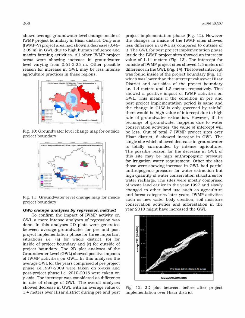
268 June 2020

shown average groundwater level change inside of IWMP project boundary in Hisar district. Only one (IWMP-V) project area had shown a decrease (0.46-2.09 m) in GWL due to high human influence and maxim farming activities. All other IWMP project areas were showing increase in groundwater level varying from 0.61-2.25 m. Other possible reason for increase in GWL may be less intense agriculture practices in these regions.

Fig. 10: Groundwater level change map for outside project boundary

Fig. 11: Groundwater level change map for inside project boundary

GWL change analyses by regression methodTo confirm the impact of IWMP activity on

GWL a more intense analyses of regression was done. In this analyses 2D plots were generated between average groundwater for pre and post project implementation phase for three important situations i.e. (a) for whole district, (b) for inside of project boundary and (c) for outside of project boundary. The 2D plot analyses of the Groundwater Level (GWL) showed positive impacts of IWMP activities on GWL. In this analyses the average GWL for the years comprised of pre project phase i.e.1997-2009 were taken on x-axis and post-project phase i.e. 2010-2016 were taken on y-axis. The intercept was considered as difference in rate of change of GWL. The overall analyses showed decrease in GWL with an average value of 1.4 meters over Hisar district during pre and post

project implementation phase (Fig. 12). However the changes in inside of the IWMP sites showed less difference in GWL as compared to outside of it. The GWL for post project implementation phase inside the IWMP project sites showed an intercept value of 1.14 meters (Fig. 13). The intercept for outside of IWMP project sites showed 1.5 meters of difference in the GWL (Fig. 14). The lowest intercept was found inside of the project boundary (Fig. 13) which was lower than the intercept valueover Hisar District and out-sides of the project boundary i.e. 1.4 meters and 1.5 meters respectively. This showed a positive impact of IWMP activities on GWL. This means if the condition in pre and post project implementation period is same and the change in GLW is only governed by rainfall there would be high value of intercept due to high rate of groundwater extraction. However, if the recharge of groundwater happens due to water conservation activities, the value of intercept will be less. Out of total 7 IWMP project sites over Hisar district, 6 showed increase in GWL. The single site which showed decrease in groundwater is totally surrounded by intense agriculture. The possible reason for the decrease in GWL of this site may be high anthropogenic pressure for irrigation water requirement. Other six sites those were showing increase in GWL had partial anthropogenic pressure for water extraction but high quantity of water conservation structures for water recharge. The sites were mostly comprised of waste land earlier in the year 1997 and slowly changed to other land use such as agriculture and forest categories later years. IWMP activities such as new water body creation, soil moisture conservation activities and afforestation in the year 2010 might have increased the GWL.

Fig. 12: 2D plot between before after project implementation over Hisar district

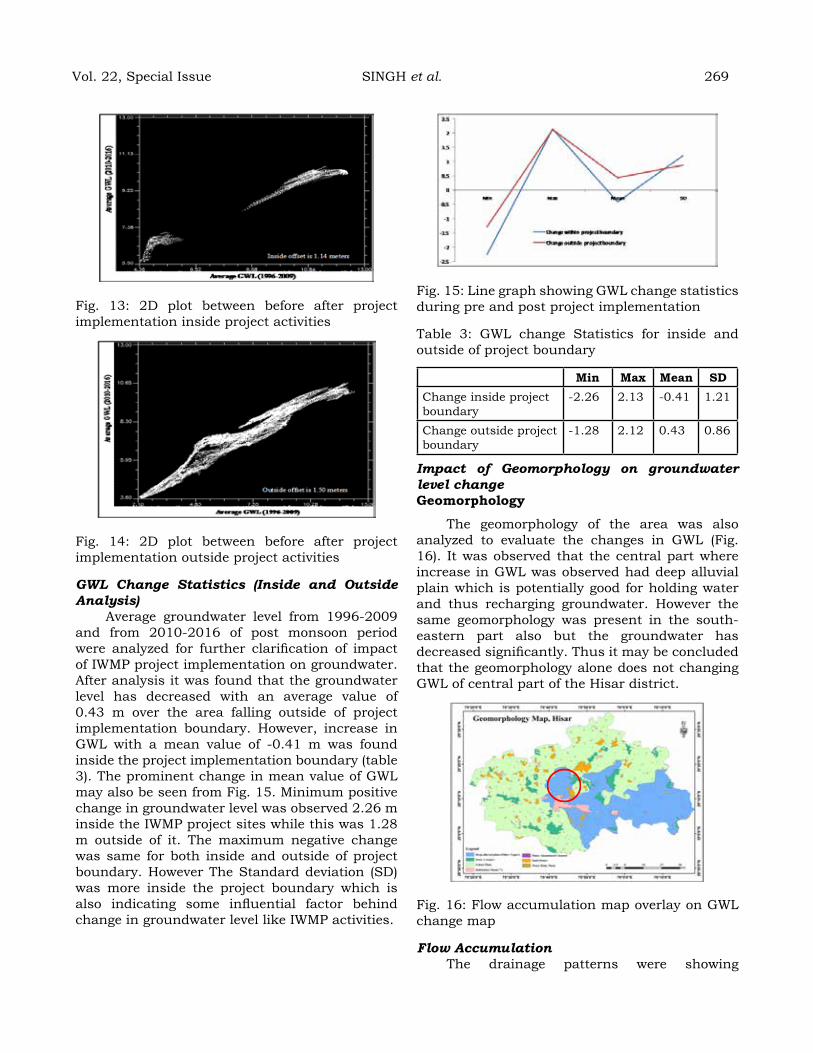
Fig. 13: 2D plot between before after project implementation inside project activities

Fig. 14: 2D plot between before after project implementation outside project activities

GWL Change Statistics (Inside and Outside Analysis)

Average groundwater level from 1996-2009 and from 2010-2016 of post monsoon period were analyzed for further clarification of impact of IWMP project implementation on groundwater. After analysis it was found that the groundwater level has decreased with an average value of 0.43 m over the area falling outside of project implementation boundary. However, increase in GWL with a mean value of -0.41 m was found inside the project implementation boundary (table 3). The prominent change in mean value of GWL may also be seen from Fig. 15. Minimum positive change in groundwater level was observed 2.26 m inside the IWMP project sites while this was 1.28 m outside of it. The maximum negative change was same for both inside and outside of project boundary. However The Standard deviation (SD) was more inside the project boundary which is also indicating some influential factor behind change in groundwater level like IWMP activities.

Fig. 15: Line graph showing GWL change statistics during pre and post project implementation

Table 3: GWL change Statistics for inside and outside of project boundary

Min Max Mean SdChange inside project boundary

-2.26 2.13 -0.41 1.21

Change outside project boundary

-1.28 2.12 0.43 0.86

Impact of Geomorphology on groundwater level changegeomorphology

The geomorphology of the area was also analyzed to evaluate the changes in GWL (Fig. 16). It was observed that the central part where increase in GWL was observed had deep alluvial plain which is potentially good for holding water and thus recharging groundwater. However the same geomorphology was present in the south-eastern part also but the groundwater has decreased significantly. Thus it may be concluded that the geomorphology alone does not changing GWL of central part of the Hisar district.

Fig. 16: Flow accumulation map overlay on GWL change map

Flow Accumulation The drainage patterns were showing


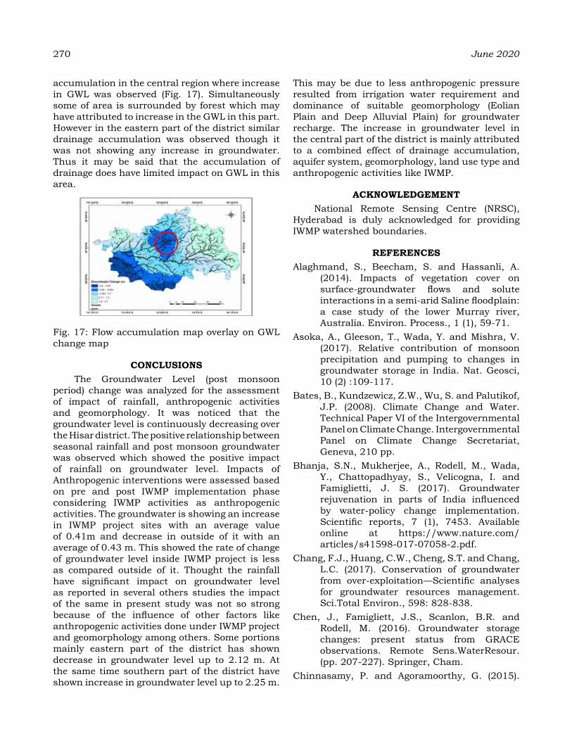
270 June 2020

accumulation in the central region where increase in GWL was observed (Fig. 17). Simultaneously some of area is surrounded by forest which may have attributed to increase in the GWL in this part. However in the eastern part of the district similar drainage accumulation was observed though it was not showing any increase in groundwater. Thus it may be said that the accumulation of drainage does have limited impact on GWL in this area.

Fig. 17: Flow accumulation map overlay on GWL change map

CoNCLuSIoNSThe Groundwater Level (post monsoon

period) change was analyzed for the assessment of impact of rainfall, anthropogenic activities and geomorphology. It was noticed that the groundwater level is continuously decreasing over the Hisar district. The positive relationship between seasonal rainfall and post monsoon groundwater was observed which showed the positive impact of rainfall on groundwater level. Impacts of Anthropogenic interventions were assessed based on pre and post IWMP implementation phase considering IWMP activities as anthropogenic activities. The groundwater is showing an increase in IWMP project sites with an average value of 0.41m and decrease in outside of it with an average of 0.43 m. This showed the rate of change of groundwater level inside IWMP project is less as compared outside of it. Thought the rainfall have significant impact on groundwater level as reported in several others studies the impact of the same in present study was not so strong because of the influence of other factors like anthropogenic activities done under IWMP project and geomorphology among others. Some portions mainly eastern part of the district has shown decrease in groundwater level up to 2.12 m. At the same time southern part of the district have shown increase in groundwater level up to 2.25 m.

This may be due to less anthropogenic pressure resulted from irrigation water requirement and dominance of suitable geomorphology (Eolian Plain and Deep Alluvial Plain) for groundwater recharge. The increase in groundwater level in the central part of the district is mainly attributed to a combined effect of drainage accumulation, aquifer system, geomorphology, land use type and anthropogenic activities like IWMP.

aCKNoWLedgeMeNtNational Remote Sensing Centre (NRSC),

Hyderabad is duly acknowledged for providing IWMP watershed boundaries.

reFereNCeSAlaghmand, S., Beecham, S. and Hassanli, A.

(2014). Impacts of vegetation cover on surface-groundwater flows and solute interactions in a semi-arid Saline floodplain: a case study of the lower Murray river, Australia. Environ. Process., 1 (1), 59-71.

Asoka, A., Gleeson, T., Wada, Y. and Mishra, V. (2017). Relative contribution of monsoon precipitation and pumping to changes in groundwater storage in India. Nat. Geosci, 10 (2) :109-117.

Bates, B., Kundzewicz, Z.W., Wu, S. and Palutikof, J.P. (2008). Climate Change and Water. Technical Paper VI of the Intergovernmental Panel on Climate Change. Intergovernmental Panel on Climate Change Secretariat, Geneva, 210 pp.

Bhanja, S.N., Mukherjee, A., Rodell, M., Wada, Y., Chattopadhyay, S., Velicogna, I. and Famiglietti, J. S. (2017). Groundwater rejuvenation in parts of India influenced by water-policy change implementation. Scientific reports, 7 (1), 7453. Available online at https://www.nature.com/articles/s41598-017-07058-2.pdf.

Chang, F.J., Huang, C.W., Cheng, S.T. and Chang, L.C. (2017). Conservation of groundwater from over-exploitation—Scientific analyses for groundwater resources management. Sci.Total Environ., 598: 828-838.

Chen, J., Famigliett, J.S., Scanlon, B.R. and Rodell, M. (2016). Groundwater storage changes: present status from GRACE observations. Remote Sens.WaterResour. (pp. 207-227). Springer, Cham.

Chinnasamy, P. and Agoramoorthy, G. (2015).

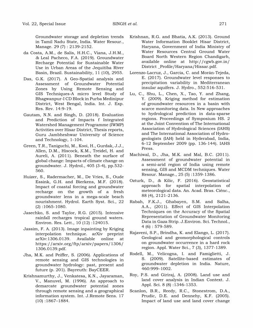
Groundwater storage and depletion trends in Tamil Nadu State, India. Water Resour., Manage. 29 (7) : 2139-2152.

da Costa, A.M., de Salis, H.H.C., Viana, J.H.M., & Leal Pacheco, F.A. (2019). Groundwater Recharge Potential for Sustainable Water Use in Urban Areas of the Jequitiba River Basin, Brazil. Sustainability, 11 (10), 2955.

Das, G.K. (2017). A Geo-Spatial analysis and Assessment of Groundwater Potential Zones by Using Remote Sensing and GIS Techniques-A micro level Study of Bhagwanpur-I CD Block in Purba Medinipur District, West Bengal, India. Int. J. Exp. Res. Rev. 14:9-19.

Gautam, N.N. and Singh, D. (2018). Evaluation and Prediction of Impacts f Integrated Watershed Management Programme (IWMP) Activities over Hisar District, Thesis reports, Guru Jambheshwar University of Science and Technology, 1-104.

Green, T.R., Taniguchi, M., Kooi, H., Gurdak, J.J., Allen, D.M., Hiscock, K.M., Treidel, H. and Aureli, A. (2011). Beneath the surface of global change: Impacts of climate change on groundwater. J. Hydrol., 405 (3-4), pp.532-560.

Huizer, S., Radermacher, M., De Vries, S., Oude Essink, G.H. and Bierkens, M.F. (2018). Impact of coastal forcing and groundwater recharge on the growth of a fresh groundwater lens in a mega-scale beach nourishment. Hydrol. Earth Syst. Sci., 22 (2) :1065-1080.

Jasechko, S. and Taylor, R.G. (2015). Intensive rainfall recharges tropical ground waters. Environ. Res. Lett., 10 (12) :124015.

Jassim, F. A. (2013). Image inpainting by Kriging interpolation technique. arXiv preprint arXiv:1306.0139. Available online at https://arxiv.org/ftp/arxiv/papers/1306/ 1306.0139.pdf.

Jha, M.K. and Peiffer, S. (2006). Applications of remote sensing and GIS technologies in groundwater hydrology: past, present and future (p. 201). Bayreuth: BayCEER.

Krishnamurthy, J., Venkatesa, K.N., Jayaraman, V., Manuvel, M. (1996). An approach to demarcate groundwater potential zones through remote sensing and a geographical information system. Int. J.Remote Sens. 17 (10) :1867–1884.

Krishnan, R.G. and Bhatia, A.K. (2013). Ground Water Information Booklet Hisar District, Haryana, Government of India Ministry of Water Resources Central Ground Water Board North Western Region Chandigarh, available online at http://cgwb.gov.in/District _Profile/Haryana/Hissar.pdf.

Lorenzo-Lacruz, J., Garcia, C. and Morán-Tejeda, E. (2017). Groundwater level responses to precipitation variability in Mediterranean insular aquifers. J. Hydro., 552:516-531.

Lu, C., Shu, L., Chen, X., Tao, Y. and Zhang, Y. (2009). Kriging method for estimation of groundwater resources in a basin with scarce monitoring data. In New approaches to hydrological prediction in data-sparse regions. Proceedings of Symposium HS. 2 at the Joint Convention of The International Association of Hydrological Sciences (IAHS) and The International Association of Hydro-geologists (IAH) held in Hyderabad, India, 6-12 September 2009 (pp. 136-144). IAHS Press.

Machiwal, D., Jha, M.K. and Mal, B.C. (2011). Assessment of groundwater potential in a semi-arid region of India using remote sensing, GIS and MCDM techniques. Water Resour. Manage., 25 (5) :1359-1386.

Ozturk, D., & Kilic, F. (2016). Geostatistical approach for spatial interpolation of meteorological data. An. Acad. Bras. Ciênc., 88 (4), 2121-2136.

Rabah, F.K.J., Ghabayen, S.M. and Salha, A.A., (2011). Effect of GIS Interpolation Techniques on the Accuracy of the Spatial Representation of Groundwater Monitoring Data in Gaza Strip. J.Environ. Sci. Technol., 4 (6) : 579-589.

Rajaveni, S.P., Brindha, K. and Elango, L. (2017). Geological and geomorphological controls on groundwater occurrence in a hard rock region. Appl. Water Sci., 7 (3), 1377-1389.

Rodell, M., Velicogna, I. and Famiglietti, J. S. (2009). Satellite-based estimates of groundwater depletion in India. Nature, 460:999–1002.

Roy, P.S. and Giriraj, A. (2008). Land use and land cover analysis in Indian Context. J. Appl. Sci. 8 (8) :1346-1353.

Scanlon, B.R., Reedy, R.C., Stonestrom, D.A., Prudic, D.E. and Dennehy, K.F. (2005). Impact of land use and land cover change


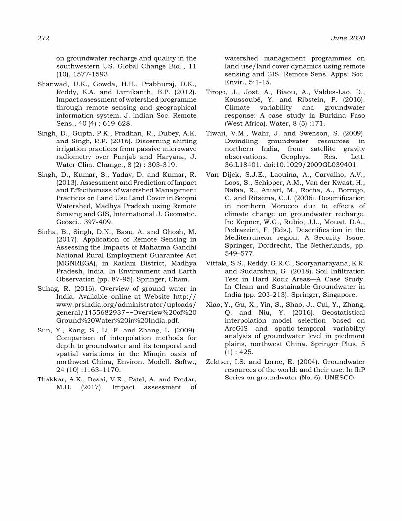
272 June 2020

on groundwater recharge and quality in the southwestern US. Global Change Biol., 11 (10), 1577-1593.

Shanwad, U.K., Gowda, H.H., Prabhuraj, D.K., Reddy, K.A. and Lxmikanth, B.P. (2012). Impact assessment of watershed programme through remote sensing and geographical information system. J. Indian Soc. Remote Sens., 40 (4) : 619-628.

Singh, D., Gupta, P.K., Pradhan, R., Dubey, A.K. and Singh, R.P. (2016). Discerning shifting irrigation practices from passive microwave radiometry over Punjab and Haryana, J. Water Clim. Change., 8 (2) : 303-319.

Singh, D., Kumar, S., Yadav, D. and Kumar, R. (2013). Assessment and Prediction of Impact and Effectiveness of watershed Management Practices on Land Use Land Cover in Seopni Watershed, Madhya Pradesh using Remote Sensing and GIS, International J. Geomatic.Geosci., 397-409.

Sinha, B., Singh, D.N., Basu, A. and Ghosh, M. (2017). Application of Remote Sensing in Assessing the Impacts of Mahatma Gandhi National Rural Employment Guarantee Act (MGNREGA), in Ratlam District, Madhya Pradesh, India. In Environment and Earth Observation (pp. 87-95). Springer, Cham.

Suhag, R. (2016). Overview of ground water in India. Available online at Website http://www.prsindia.org/administrator/uploads/general/1455682937~~Overview%20of%20Ground%20Water%20in%20India.pdf.

Sun, Y., Kang, S., Li, F. and Zhang, L. (2009). Comparison of interpolation methods for depth to groundwater and its temporal and spatial variations in the Minqin oasis of northwest China, Environ. Modell. Softw., 24 (10) :1163–1170.

Thakkar, A.K., Desai, V.R., Patel, A. and Potdar, M.B. (2017). Impact assessment of

watershed management programmes on land use/land cover dynamics using remote sensing and GIS. Remote Sens. Apps: Soc. Envir., 5:1-15.

Tirogo, J., Jost, A., Biaou, A., Valdes-Lao, D., Koussoubé, Y. and Ribstein, P. (2016). Climate variability and groundwater response: A case study in Burkina Faso (West Africa). Water, 8 (5) :171.

Tiwari, V.M., Wahr, J. and Swenson, S. (2009). Dwindling groundwater resources in northern India, from satellite gravity observations. Geophys. Res. Lett. 36:L18401. doi:10.1029/2009GL039401.

Van Dijck, S.J.E., Laouina, A., Carvalho, A.V., Loos, S., Schipper, A.M., Van der Kwast, H., Nafaa, R., Antari, M., Rocha, A., Borrego, C. and Ritsema, C.J. (2006). Desertification in northern Morocco due to effects of climate change on groundwater recharge. In: Kepner, W.G., Rubio, J.L., Mouat, D.A., Pedrazzini, F. (Eds.), Desertification in the Mediterranean region: A Security Issue. Springer, Dordrecht, The Netherlands, pp. 549–577.

Vittala, S.S., Reddy, G.R.C., Sooryanarayana, K.R. and Sudarshan, G. (2018). Soil Infiltration Test in Hard Rock Areas—A Case Study. In Clean and Sustainable Groundwater in India (pp. 203-213). Springer, Singapore.

Xiao, Y., Gu, X., Yin, S., Shao, J., Cui, Y., Zhang, Q. and Niu, Y. (2016). Geostatistical interpolation model selection based on ArcGIS and spatio-temporal variability analysis of groundwater level in piedmont plains, northwest China. Springer Plus, 5 (1) : 425.

Zektser, I.S. and Lorne, E. (2004). Groundwater resources of the world: and their use. In IhP Series on groundwater (No. 6). UNESCO.

Storage behaviour of pear fruit in response to putrescine application at room temperature

veerPartaP SINgh*, S.K. JaWaNdha aNd P.P.S. gILLDepartment of Fruit Science, Punjab Agricultural University Ludhiana, 141004, Punjab (India)

*Corresponding author E-mail: [email protected]

aBStraCtInvestigations were carried out to examine the putrescine (PUT) application effect on storage behaviour of pear fruit beneath ambient circumstances. PUT treatments of 1mM, 2mM & 3mM were given one week before harvest on pear cv. Punjab Beauty. Treated fruit were packed in CFB boxes and kept at room temperature (31 ± 2.8oC, 78 ± 5% RH) for storage studies. Fruit samples were analysed for various physico-chemical and enzymatic activities on 0, 3, 6, 9, 12 and 15th day of storage. During storage, a significant reduction in weight loss, spoilage, titratable acidity and starch content was recorded in 2mM & 3mM PUT treated fruit compared with control. Sensory quality, fruit firmness and soluble solids content (SSC) of fruit were also retained highest in 2mM & 3mM putrescine treated fruit at storage terminal. Enzymatic activities liked pectin methyl esterase (PME) and cellulase recorded to be lower in PUT treated fruit. It can be summarised that 2mM & 3mM PUT applications were effectual in keeping the post-harvest quality of pear fruit up to 12 days at ambient conditions.

Key Word: Pear, putrescine, quality, room temperature, storage life

INtroduCtIoN

Pear (Pyrus spp.) is the most vitaltemperate region pome fruits. Its delicious taste, crispy nature with grit cells and nutritive value makes it table purpose fruit with good eating quality (Colaric et al., 2007). Pear matures in the high temperature conditions of sub-tropics of North-Western India when both temperature as well as humidity is very high which reduces the shelf life of fruit under ambient conditions. Moreover, pears are climacteric in nature and during lengthy storage period, fruit are vulnerable to different postharvest disorders (Villalobos-Acuna and Mitcham, 2008). Hence, betterment of the storage potentialis the keyconcern for the growers.

Being climacteric in nature, fruit remain biologically active and continues transpiration and respiration accompanied with sudden rise in ethylene production during storage which leads to sever postharvest losses (Wills et al., 2007), whilst polyamines are proved to be vastly effectual to reduce the postharvest losses due to their antagonistic nature towards ripening after harvest of climacteric fruit (Valero et al., 2002). Among polyamines, PUT is predominant naturally occurring positively charged aliphatic amine with low molecular weight is an anti-ethylene compound being competitor of ethylene precursor (1-ACC) (Apelbaum et al., 1981). In earlier studies on fruit, the role of PUT in

extending the shelf life and maintaining the fruit quality is well incorporated. However, to outflank of our awareness not any information is available on the effect of preharvest PUT application in extending the shelf life in subtropical pear. Therefore, the current experiment was conducted to enhancement the shelf life of pear fruit cv. Punjab Beauty with preharvest PUT application at ambient conditions.

MaterIaL aNd MethodSPreharvest PUT applications @ 1mM, 2mM

& 3mM and water (control) were given 1 week before harvest to uniform and healthy plants of pear cv. Punjab Beauty at Fruit Research Farm, Punjab Agricultural University, Ludhiana (30.91oN, 75.85oE). Fruits were harvested at proper stage of maturity (134 days fromsetting fruit setting) and directly transported to the Post-Harvest Laboratory for further shelf life study. Before storage at ambient circumstances (31 ± 2.8oC, 78 ± 5% RH), fruits were disinfected with 100 ppm chlorination solution and then packed in 3ply CFB boxes (5% perforation) with layer of paper. One kg fruit from each four replications of each treatment was packed for various analyses. Periodical observations for physico-chemical and enzymatic activities were made on 0, 3, 6, 9, 12 and 15 days of storage.


274 June 2020

Observations recordedWeight loss during storage was recorded

using an electronic balance on the initial weight basis with respect to fruit weight after 3 days interval and recorded in per cent. The fruit firmness was recorded by using stand mounted Penetrometer (Model FT-327, USA) having 8mm stainless steel probe after removing the fruit’s peel and expressed in Newton (N) force. Sensory quality of the fruit was evaluated on the base of aroma, freshness, texture, taste and colour by following the 9-point hedonic scale (Amerine et al., 1965). Spoilage per cent was deliberated on the spoiled fruits number basewith total fruits and expressed in percentage.SSC was measured by using digital hand refracto meter (ATAGO) in unit per cent. Titratable acidity was estimated by titer 2 ml juice with 2 drops phenolphthalein (indicator) against 0.1 N NaOH and expressed in per cent malic acid. Starch content was determined as per the method described by Stevens and Chapman, (1955). The enzymatic activities of PME and cellulase were measured as per the method given by (Mahadevan and Sridhar, 1982).

Experimental design and statistical analysisThe experiment was performed in 2016

& 2017 year and laid out in CRD having 4 replications of each treatment. The pooled data were analysis with one-way analysis of variance (ANOVA) & means of data were alienated with LSD test. Differences were regarded significant (p≤0.05) with statistical software SAS (version 9.3 for windows). Data were written as mean ± standard error.

reSuLtS aNd dISCuSSIoNWeight loss along storage was significantly

enhanced in all the treated fruit during the entire storage (Table 1A). Loss in weight during storage is mainly because of transpiration of water through the fruit’s surface. However, PUT treatment of 2mM & 3mM were found to be highly effective to diminish the loss in weight along storage and these treatments recorded 8.54% & 11.28% lower weight loss compared with control respectively at the storage last. The reduction in loss in weight of PUT treated fruit represents the maintenance of turgidity and freshness of the fruit. PUT affect the respiration process by suppressing the ethylene production because PUT is antagonist to production of ethylene as both mutually compete for the single precursor i.e. L-amino cyclopropane-L-carboxylic acid (Apelbaum et

al., 1981) and helps to retain cell turgidity and reduces transpiration losses. Similar to these findings, PUT also effectively lowered the weight loss of kiwifruit during the storage as compared with control (Valero et al., 2002). A considerable firmness reduction was observed in all PUT treated fruit through storage (Table 1B). Although, fruit looses firmness during the storage while fruit treated with PUT registered higher firmness over the control. At the storage last, 2mM & 3mM PUT treated fruit retained 38.04% & 40.02% higher firmness, respectively compared with the control. In another study, Mirdehghan and Rahimi, (2016) revealed that polyamines application (putrescine and spermine) significantly delayed the grapes softening, whereas control fruits exhibited the sharp decline in firmness. Putrescine consisting of two amino groups is a natural positively charged biogenic amine strongly binds to various proteins; phospholipids, nucleic acids and others negatively charged molecules which maintain the fruit firmness (Champa et al., 2014).

Results elucidated that sensory quality of pear fruit improved along storage with non-significant differences till 6 day of storage (Table 1C). Sensory quality in 3mM PUT treated fruit increased to the 9th storage day and then after, it declined in all PUT treatments till the end of storage. High sensory quality for a longer duration of storage in PUT treatment might be due to the reduced rate of respiration that led to the high availability of polysaccharides compared with control (Valero et al., 2002). Similarly, PUT treated mango fruit retained excellent quality after three weeks of storage compared with control (Jawandha et al., 2012). Fruit spoilage significantly increased along the storage of fruit (Table 1D). PUT treatment had considerable effect on the fruit spoilage as no fruit was spoiled till 9 storage days, while control fruit showed 2.10% spoilage. On the 12th & 15th day of storage, fruit from the all treatments showed spoilage. At the end of storage, minimum spoilage of 3.09% was recorded in 3mM PUT treated fruit while highest in control. Likewise, Jawandha et al., (2012) studied the putrescine effect on fruit spoilage of mango cv. Langra and found lowest spoilage in 2mM PUT treatment. The PUT treatment delayed the senescence and decay incidence which could be ascribed to the anti-pathogenic properties.

Data given in Fig. 1A elucidated that SSC of fruit initially increased and then decreased at later stages in all the treatments. SSC increased

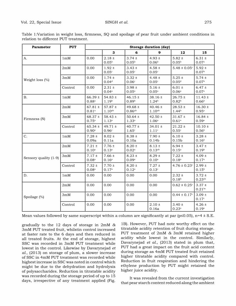
Table 1:Variation in weight loss, firmness, SQ and spoilage of pear fruit under ambient conditions in relation to different PUT treatment.

Parameter Put Storage duration (day) 3 6 9 12 15

A. 1mM 0.00 2.18 ± 0.05b

3.74 ± 0.05b

4.93 ± 0.06b

5.82 ± 0.05b

6.31 ± 0.07a

Weight loss (%)

2mM 0.00 1.92 ± 0.05c

3.43 ± 0.05c

4.58 ± 0.05c

5.48 ± 0.05c 5.92 ± 0.07b

3mM 0.00 1.74 ± 0.04d

3.32 ± 0.06c

4.48 ± 0.05c

5.25 ± 0.05d

5.74 ± 0.07b

Control 0.00 2.31 ± 0.04a

3.98 ± 0.05a

5.16 ± 0.05a

6.01 ± 0.06a

6.47 ± 0.07a

B. 1mM 66.39 ± 0.88a

54.83 ± 1.19b

46.15 ± 0.89b

38.16 ± 1.24b

26.75 ± 0.82b

11.43 ± 0.66b

Firmness (N)

2mM 67.81 ± 0.81a

57.87 ± 1.10ab

49.68 ± 0.86ab

40.46 ± 1.10ab

28.53 ± 1.44b

16.30 ± 0.95a

3mM 68.37 ± 0.75a

58.43 ± 1.13a

50.64 ± 1.33a

42.50 ± 1.06a

31.67 ± 0.61a

16.84 ± 0.59a

Control 65.34 ± 0.90a

49.71 ± 0.96c

40.77 ± 1.65c

34.01 ± 1.11c

21.22 ± 0.55c

10.10 ± 0.56b

C. 1mM 7.28 ± 0.09a

8.02 ± 0.11a

8.38 ± 0.10a

7.90 ± 0.14b

6.10 ± 0.15b

3.28 ± 0.16b

Sensory quality (1-9)

2mM 7.21 ± 0.10a

7.76 ± 0.13a

8.20 ± 0.02a

8.13 ± 0.13ab

6.94 ± 0.15a

3.47 ± 0.19b

3mM 7.17 ± 0.08a

7.66 ± 0.16a

8.23 ± 0.09a

8.29 ± 0.10a

7.22 ± 0.18a

4.09 ± 0.17a

Control 7.32 ± 0.08a

7.70 ± 0.17a

8.20 ± 0.12a

7.27 ± 0.13c

4.76 ± 0.23c 2.99 ± 0.15b

D. 1mM 0.00 0.00 0.00 0.00 2.32 ± 0.18b

3.72 ± 0.23ab

Spoilage (%)

2mM 0.00 0.00 0.00 0.00 0.62 ± 0.25c 3.37 ± 0.21bc

3mM 0.00 0.00 0.00 0.00 0.44 ± 0.17c 3.09 ± 0.17c

Control 0.00 0.00 0.00 2.10 ± 0.16a

3.40 ± 0.23a

4.26 ± 0.19a

Mean values followed by same superscript within a column are significantly at par (p≤0.05), n=4 ± S.E.

gradually to the 12 days of storage in 2mM & 3mM PUT treated fruit, whilstin control increased at faster rate to the 6 days and then reduced in all treated fruits. At the end of storage, highest SSC was recorded in 3mM PUT treatment while lowest in the control. Likewise by Davarynejad et al., (2013) on storage of plum, a slower increase of SSC in 4mM PUT treatment was recorded while highest increase in SSC was noted in control which might be due to the dehydration and hydrolysis of polysaccharides. Reduction in titratable acidity was recorded during the storage period of up to 15 days, irrespective of any treatment applied (Fig.

1B). However, PUT had note worthy effect on the titratable acidity retention of fruit during storage. PUT treatment of 2mM & 3mM retained higher acidity while lowest in the control. Similarly, Davarynejad et al., (2013) stated in plum that, PUT had a great impact on the fruit acid content during storage as 4mM PUT treated fruit retained higher titratable acidity compared with control. Reduction in fruit respiration and hindering the ethylene production by PUT might retained the higher juice acidity.

It was revealed from the current investigation that pear starch content reduced along the ambient


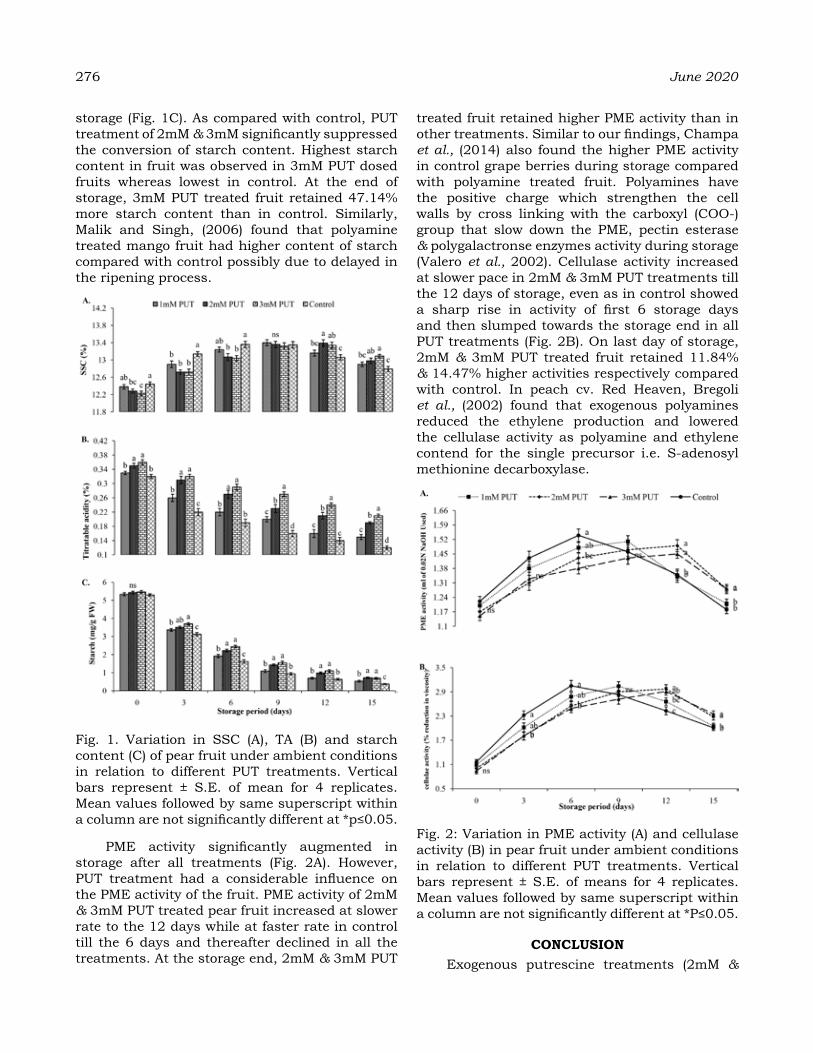
276 June 2020

storage (Fig. 1C). As compared with control, PUT treatment of 2mM & 3mM significantly suppressed the conversion of starch content. Highest starch content in fruit was observed in 3mM PUT dosed fruits whereas lowest in control. At the end of storage, 3mM PUT treated fruit retained 47.14% more starch content than in control. Similarly, Malik and Singh, (2006) found that polyamine treated mango fruit had higher content of starch compared with control possibly due to delayed in the ripening process.

Fig. 1. Variation in SSC (A), TA (B) and starch content (C) of pear fruit under ambient conditions in relation to different PUT treatments. Vertical bars represent ± S.E. of mean for 4 replicates.Mean values followed by same superscript within a column are not significantly different at *p≤0.05.

PME activity significantly augmented in storage after all treatments (Fig. 2A). However, PUT treatment had a considerable influence on the PME activity of the fruit. PME activity of 2mM & 3mM PUT treated pear fruit increased at slower rate to the 12 days while at faster rate in control till the 6 days and thereafter declined in all the treatments. At the storage end, 2mM & 3mM PUT

treated fruit retained higher PME activity than in other treatments. Similar to our findings, Champa et al., (2014) also found the higher PME activity in control grape berries during storage compared with polyamine treated fruit. Polyamines have the positive charge which strengthen the cell walls by cross linking with the carboxyl (COO-) group that slow down the PME, pectin esterase & polygalactronse enzymes activity during storage (Valero et al., 2002). Cellulase activity increased at slower pace in 2mM & 3mM PUT treatments till the 12 days of storage, even as in control showed a sharp rise in activity of first 6 storage days and then slumped towards the storage end in all PUT treatments (Fig. 2B). On last day of storage, 2mM & 3mM PUT treated fruit retained 11.84% & 14.47% higher activities respectively compared with control. In peach cv. Red Heaven, Bregoli et al., (2002) found that exogenous polyamines reduced the ethylene production and lowered the cellulase activity as polyamine and ethylene contend for the single precursor i.e. S-adenosyl methionine decarboxylase.

Fig. 2: Variation in PME activity (A) and cellulase activity (B) in pear fruit under ambient conditions in relation to different PUT treatments. Vertical bars represent ± S.E. of means for 4 replicates.Mean values followed by same superscript within a column are not significantly different at *P≤0.05.

CoNCLuSIoNExogenous putrescine treatments (2mM &

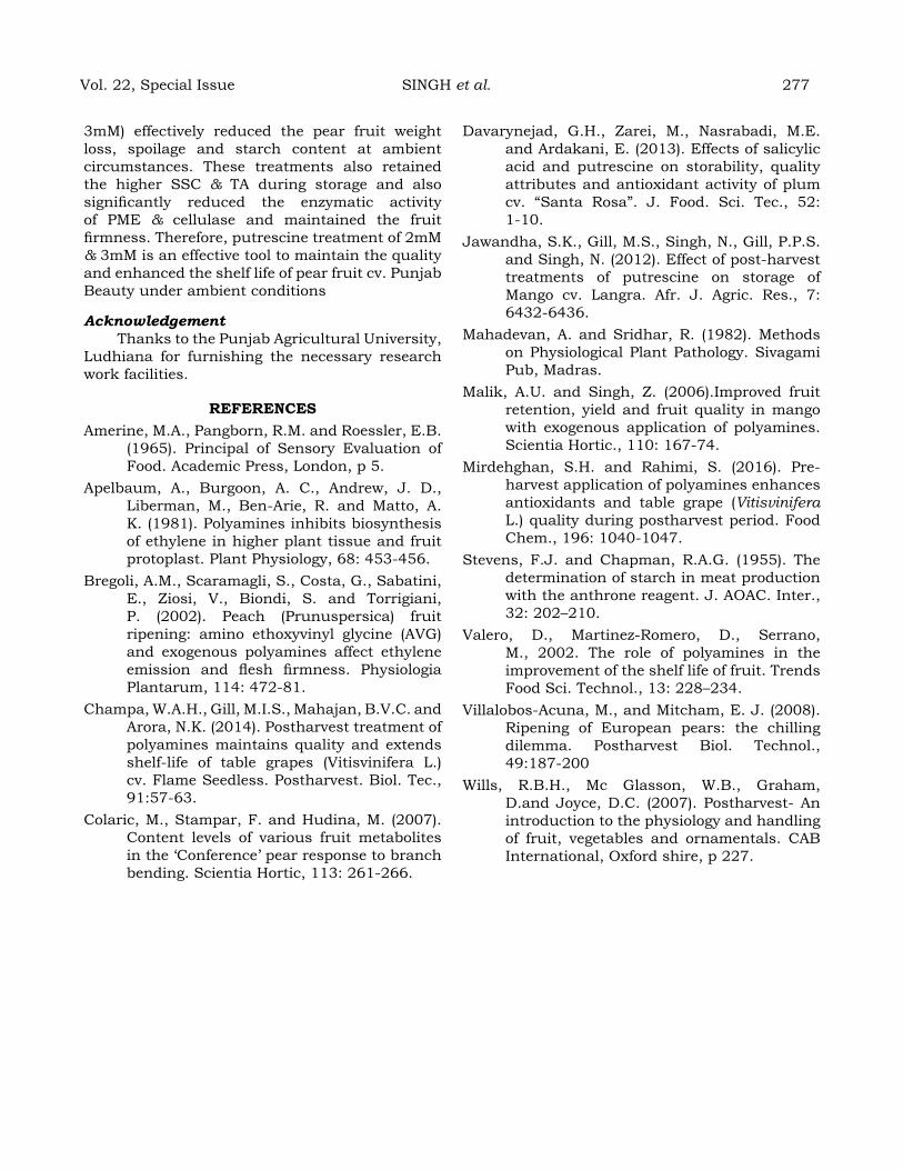
3mM) effectively reduced the pear fruit weight loss, spoilage and starch content at ambient circumstances. These treatments also retained the higher SSC & TA during storage and also significantly reduced the enzymatic activity of PME & cellulase and maintained the fruit firmness. Therefore, putrescine treatment of 2mM & 3mM is an effective tool to maintain the quality and enhanced the shelf life of pear fruit cv. Punjab Beauty under ambient conditions

AcknowledgementThanks to the Punjab Agricultural University,

Ludhiana for furnishing the necessary research work facilities.

reFereNCeSAmerine, M.A., Pangborn, R.M. and Roessler, E.B.

(1965). Principal of Sensory Evaluation of Food. Academic Press, London, p 5.

Apelbaum, A., Burgoon, A. C., Andrew, J. D., Liberman, M., Ben-Arie, R. and Matto, A. K. (1981). Polyamines inhibits biosynthesis of ethylene in higher plant tissue and fruit protoplast. Plant Physiology, 68: 453-456.

Bregoli, A.M., Scaramagli, S., Costa, G., Sabatini, E., Ziosi, V., Biondi, S. and Torrigiani, P. (2002). Peach (Prunuspersica) fruit ripening: amino ethoxyvinyl glycine (AVG) and exogenous polyamines affect ethylene emission and flesh firmness. Physiologia Plantarum, 114: 472-81.

Champa, W.A.H., Gill, M.I.S., Mahajan, B.V.C. and Arora, N.K. (2014). Postharvest treatment of polyamines maintains quality and extends shelf-life of table grapes (Vitisvinifera L.) cv. Flame Seedless. Postharvest. Biol. Tec., 91:57-63.

Colaric, M., Stampar, F. and Hudina, M. (2007). Content levels of various fruit metabolites in the ‘Conference’ pear response to branch bending. Scientia Hortic, 113: 261-266.

Davarynejad, G.H., Zarei, M., Nasrabadi, M.E. and Ardakani, E. (2013). Effects of salicylic acid and putrescine on storability, quality attributes and antioxidant activity of plum cv. “Santa Rosa”. J. Food. Sci. Tec., 52: 1-10.

Jawandha, S.K., Gill, M.S., Singh, N., Gill, P.P.S. and Singh, N. (2012). Effect of post-harvest treatments of putrescine on storage of Mango cv. Langra. Afr. J. Agric. Res., 7: 6432-6436.

Mahadevan, A. and Sridhar, R. (1982). Methods on Physiological Plant Pathology. Sivagami Pub, Madras.

Malik, A.U. and Singh, Z. (2006).Improved fruit retention, yield and fruit quality in mango with exogenous application of polyamines.Scientia Hortic., 110: 167-74.

Mirdehghan, S.H. and Rahimi, S. (2016). Pre-harvest application of polyamines enhances antioxidants and table grape (Vitisvinifera L.) quality during postharvest period. Food Chem., 196: 1040-1047.

Stevens, F.J. and Chapman, R.A.G. (1955). The determination of starch in meat production with the anthrone reagent. J. AOAC. Inter., 32: 202–210.

Valero, D., Martinez-Romero, D., Serrano, M., 2002. The role of polyamines in the improvement of the shelf life of fruit. Trends Food Sci. Technol., 13: 228–234.

Villalobos-Acuna, M., and Mitcham, E. J. (2008).Ripening of European pears: the chilling dilemma. Postharvest Biol. Technol., 49:187-200

Wills, R.B.H., Mc Glasson, W.B., Graham, D.and Joyce, D.C. (2007). Postharvest- An introduction to the physiology and handling of fruit, vegetables and ornamentals. CAB International, Oxford shire, p 227.


Journal of AgrometeorologyVolume 22 Special Issue June, 2020

Peer reviewed papers presented at International Symposium on “Advances in Agrometeorology for managing

Climatic Risks of Farmers” at Jawaharlal Nehru University, New Delhi, during 11-13 February, 2019. The

International Symposium was organised jointly by Association of Agrometeorologists (Delhi Chapter), Indian

Council of Agricultural Research- Indian Agricultural Research Institute (ICAR-IARI), India Meteorological

Department (IMD) and Jawaharlal Nehru University (JNU), New Delhi.

Special Editorial Board

Dr. SC Bhan

Scientist 'F'Agromet Advisory Service DivisionIMD, New Delhi

Dr. KK Singh

Scientist 'G' and HeadAgromet Advisory Service Division

IMD, New Delhi

Dr. DK. Das

Principal ScientistDivision of Agricultural PhysicsICAR-IARINew Delhi

Dr. SD Attri

Scientist 'F'Agromet Advisory Service Division

IMD, New Delhi

Dr. HS Shivaramu

Professor and HeadAgrometeorology sectionCollege of Agriculture, UAS, GKVK, Bangalore

Dr. Ram Niwas

ProfessorDeptt. of Agricultural Meteorology

College of Agriculture,CCSHAU, Hisar

Mrs. Mehnaj Tharranum. A

Project Scientist 'C'IMD, New Delhi

Dr. Mahender Singh

Sr. ScientistAgromet Research Centre, Chatha,

SKUAST- Jammu

We, the editors of this special issue, thank the executive council of

Association of Agrometeorologists for providing this great opportunity to

edit the “Journal of Agrometeorology, INAGMET 2019: Special Issue”.

We sincerely acknowledge the authors for their timely submission and

correction of manuscript.

We thankfully acknowledge the eminent reviewers for their excellent and

timely cooperation, to bring out the technically perfect manuscript.

We also thank Mrs. Ch. Sridevi, and the entire research staff of Agromet

Advisory Service Division of India Meteorological Department for

checking the references and typographical errors in the manuscript.

Financial support provided by NABARD for bringing out this special

issue is thankfully acknowledged.

Journalof

Agrometeorology

Special IssueINAGMET 2019

June, 2020Volume 22

Acknowledgement

GLIMPSES OF - 2019INAGMET GLIMPSES OF - 2019INAGMET

Journal of

Agrometeorology

Volume 22 Special Issue June, 2020


Published by Association of Agrometeorologists (Delhi Chapter), India Meteorological Department, Lodhi Road, New Delhi-110003, India and printed at Quick Digital Print Services, Kotla Mubarakpur, New Delhi, India.

Journ

al o

f Agro

mete

oro

logy

Volu

me 2

2 S

pecia

l Issue J

une, 2

02

0

Journal - Home | Association of Agrometeorologists

Documents

Transcript of Journal - Home | Association of Agrometeorologists