JOURNAL - GitHub Pages · JOURNAL Volume 6, Number 1 Winter 2005 RISKMETRICS › Distribution of...
89
JOURNAL Volume 6, Number 1 Winter 2005 RISKMETRICS › Distribution of Defaults in a Credit Basket › Risk Budgeting for Pension Plans › Incorporating Equity Derivatives into the CreditGrades ™ Model › Adaptations of Monte Carlo Simulation Techniques to American Option Pricing
-
Upload
trinhthien -
Category
Documents
-
view
212 -
download
0
Transcript of JOURNAL - GitHub Pages · JOURNAL Volume 6, Number 1 Winter 2005 RISKMETRICS › Distribution of...

JOURNALVolume 6, Number 1 Winter 2005
R I S K M E T R I C S
› Distribution of Defaults in a Credit Basket
› Risk Budgeting for Pension Plans
› Incorporating Equity Derivatives into theCreditGrades™ Model
› Adaptations of Monte Carlo SimulationTechniques to American Option Pricing

JOURNALVolume 6, Number 1 Winter 2005
R I S K M E T R I C S
3 Distribution of Defaults in a Credit Basket
9 Risk Budgeting for Pension Plans
35 Incorporating Equity Derivatives into theCreditGrades™ Model
65 Adaptations of Monte Carlo SimulationTechniques to American Option Pricing
COVER ARTTerm structure output: Yield plotted against maturity.RiskMetrics Journal, Spring 2001; Vol. 2, No. 1; pg 29
www.riskmetrics.com

1
Editor’s NoteChristopher C. Finger
RiskMetrics [email protected]
As the year 2005 draws to a close, we are pleased to bring you the latest issue of the RiskMetrics
Journal. The articles in this issue represent work we have undertaken in an effort to continue to
broaden our coverage of risks and instruments, and to expand the application of risk measures into
more active decision-making tasks.
The first article, a short note by Pete Benson, presents an interesting special case of the standard
credit portfolio derivatives pricing model. Closed-form solutions are in short supply for these
models, particularly for non-trivial values for correlation. Pete noticed this somewhat surprising
result in preparing examples of the model. Once he found the proof, Pete proceeded to challenge a
number of the research group members with the problem, and the problem has now become a standard
interview question here.
In the second article, Jorge Mina provides the third in a series of articles, begun in the Winter
2003 issue, relating to the theme of risk attribution. In the previous articles, we have presented risk
attribution schemes for equity and fixed income portfolios by first describing the relevant
performance attribution schemes, and then defining the risk attribution schemes in parallel. Jorge
extends this body of work by presenting methods for risk budgeting that rely on risk attribution as
a key input. Ultimately, the goal is to build a framework wherein risk is budgeted as any scarce
resource, and a portfolio manager can make active investments whose sizes are appropriate to the
manager’s confidence in his views.
Also extending previous work, Robert Stamicar and Christopher Finger present an extension of the
CreditGrades model which allows for joint pricing of credit and equity derivatives. We had
examined the use of implied volatility in the CreditGrades model in 2002, and presented some of
these results in the CreditGrades Technical Document. The framework here is more robust,
c©2005 RiskMetrics Group, Inc. All Rights Reserved.

2 Editor’s Note
however, in that it makes the appropriate adjustments to the standard Black-Scholes volatilities;
these adjustments are necessary since under the CreditGrades model, the firm’s assets, but not its
equity, evolve as a lognormal process. Robert and Christopher take advantage of this framework to
investigate a variety of combinations of fundamental and market-based inputs to CreditGrades, and
illustrate the approaches through examples on four individual firms.
In our final article, Serena Agoro-Menyang presents a survey of Monte Carlo methods to price
American options. As Serena points out in her introduction, standard Monte Carlo techniques are
not well suited for this problem since they are fundamentally forward algorithms: at a given point
in time, we know about the past evolution of the option underlying, but not about its future. This
complicates the valuation of American options, since it is difficult to determine when it is optimal
to exercise. Backward induction techniques are attractive for American option pricing, in that we
have seen information about the future evolution of the underlying, and therefore know when it is
optimal to exercise. Unfortunately, these algorithms typically come with a large computational
burden. The approaches that Serena surveys attempt to blend the computational benefits of Monte
Carlo with the applicability of the backward induction techniques.
As always, we look forward to your comments and questions. Please feel free to correspond with
the authors directly, or through your RiskMetrics Group representative.

3
Distribution of Defaults in a Credit Basket: AnInteresting Special Case
Pete BensonRiskMetrics Group
The Gaussian copula model of a credit basket of correlated names typically requires numericalmethods when correlation is other than zero or one. We expose an interesting special case with asimple closed-form solution.
1 Introduction
In this paper, we present a very simple closed-form solution to the behavior of a credit basket for
an interesting special case of a widely used basket model. This special case is interesting because
the correlation between the names is between zero and one, a situation typically handled by more
complex techniques (Monte Carlo or semi-analytic methods). Even a single closed-form solution is
handy because it allows us to check the results from the more complex methods.
As with all derivatives, pricing and risk analysis require a model for the behavior of the
underlying. The Gaussian copula model for the credit basket assumes that for a horizon t , a name
experiences a credit event if the name’s lognormal asset return at t falls below some event
threshold. For each name k, we must know the probability of a credit event, pk. If we assume
asset log returns are normal, then the event threshold corresponding to pk is �−1(pk) standard
deviations.
We also need to represent correlation between the asset returns of the names. A simplifying
assumption is that there is a single correlation parameter, ρ, that represents the correlation between
every pair of distinct names. Given the pk and ρ, we can then calculate the probability distribution
of the number of defaults, N .
Because it is part of the special case we alluded to at the beginning, we will henceforth assume
that all the pk have the same value, p.

4 Distribution of Defaults in a Credit Basket: An Interesting Special Case
If the names are independent (ρ is zero), N has a binomial distribution. So, for example, if we
have ten independent names, and the probability of an individual name defaulting is 30%, the
distribution of defaults is as shown in Figure 1.
Figure 1
Event distribution for ten independent names, default probability 30%
expected loss
27.90% 1.98% 0.12%
0%
5%
10%
15%
20%
25%
30%
0 1 2 3 4 5 6 7 8 9 10
Pro
bab
ilit
y
There is also a closed-form solution if asset returns are perfectly correlated. Figure 2 illustrates this
case when names default with probability 30%.
Figure 2
Event distribution for ten names, ρ = 100%, default probability 30%
0%
10%
20%
30%
40%
50%
60%
70%
80%
0 1 2 3 4 5 6 7 8 9 10
Number of credit events
Pro
bab
ilit
y

The special case 5
Handling correlation between zero and one is usually more difficult. Even if the event probability
is the same for all names, there is no closed-form solution for an arbitrary correlation between
names.
The typical approach is to treat this problem with a single-factor market model. If the correlation
between asset returns of any two names is ρ, then we can represent the return on name k with
Rk = √ρM + √
1 − ρZk, (1)
where M is the return on the market variable, and Zk is standard normal noise, idiosyncratic to
name k. Name k defaults if Rk < �−1(p).
At this point, a simple approach would be to carry out Monte Carlo simulation on M and the Zk.
Each Monte Carlo trial would then yield a value for the Rk. The Rk in turn would be compared
to the event threshold to determine whether name k defaulted.
A better approach is to exploit the fact that this is a single factor model, and condition on M . If
M = m is known, but the Zk are not, then credit events are independent. A name defaults if
Rk = √ρm + √
1 − ρZk < �−1(p). Rearranging, a name defaults if Zk <�−1(p)−m
√ρ√
1−ρ. This happens
with probability
p(m) = �
(�−1(p) − m
√ρ√
1 − ρ
). (2)
Since the names all default independently with equal probability, the distribution of defaults is
again binomial. For n names, the probability of j events is
Pr[N = j |M = m] =(
n
j
)p(m)j (1 − p(m))n−j .
We can eliminate m:
Pr[N = j ] =(
n
j
) ∞∫−∞
p(m)j (1 − p(m))n−j φ(m)dm. (3)
Typically, a quadrature method is required. Figure 3 shows the distribution for correlation of 50%
and default probability 30%.

6 Distribution of Defaults in a Credit Basket: An Interesting Special Case
Figure 3
Event distribution for ten names, ρ = 50%, default probability 30%
0%
5%
10%
15%
20%
25%
30%
0 1 2 3 4 5 6 7 8 9 10
Number of credit events
Pro
bab
ilit
y
2 The special case
Now, what is this special case we mentioned at the outset? There are a number of ways to
motivate it, but let us consider Equation (2). It would be much easier to deal with if �−1(p) = 0.
This happens for p = 1/2. Now Equation (2) becomes
p(m) = �
(−m
√ρ
1 − ρ
).
In fact, this would be even simpler if ρ = 1/2, so that
p(m) = �(−m) = 1 − �(m).
Now (3) becomes
Pr[N = j ] =(
n
j
) ∞∫−∞
(1 − �(m))j �(m)n−jφ(m)dm.
Since φ is the derivative of �, we can substitute u = �(m) to obtain
Pr[N = j ] =(
n
j
) 1∫0
(1 − u)jun−j du.

Summary 7
This is just the integral of a polynomial! In fact, it is the Eulerian integral of the first kind, or
beta integral, with solution B(n − j + 1, j + 1). But there’s a more subtle and intuitive approach.
With a little insight, a simple expression for Pr[N = j ] reveals itself.
With p = 1/2 and ρ = 1/2, let us set aside the calculus, and consider the original factor model
given in (1). This becomes
Rk = √1/2(M + Zk).
Recall that name k defaults if Rk < 0. Equivalently, name k defaults if M < −Zk. If we substitute
M∗ = −M , then name k defaults if M∗ > Zk.
Now, what is the probability that M∗ is greater than exactly j of the Zk? If we observe M and
the Zk, and sort the observations into an ascending list, we see that this is the same as asking for
the probability that the observation of M∗ is the j th largest number. M and the Zk are identically
distributed, continuous random variables. Consequently, M is equally likely to be in any position in
the list. Since there are n + 1 positions in the list, we have
Pr[N = j ] = 1
n + 1,
for each j . Figure 4 drives the point home visually. The distribution is flat, regardless of n.
Figure 4
Event distribution for ten names, ρ = 50%, default probability 50%
0%
5%
10%
0 1 2 3 4 5 6 7 8 9 10
Number of credit events
Pro
bab
ilit
y

8 Distribution of Defaults in a Credit Basket: An Interesting Special Case
3 Summary
So, we have this result:
Assume a credit basket of n names, with asset correlation of 0.5 between any pair,
and each name defaulting with probability 0.5. Then the number of defaults is
evenly distributed, with the probability of having exactly 0, 1, 2, ..., or n defaults
being 1n+1 in each case.
We should note that we did not actually come across this quite as described above. While playing
around with a semi-analytic solution, we observed how the distribution shape changed as we
changed the inputs. A little experimentation led to the discovery of the flat (uniform) distribution
described here. From there, we went looking for a simple proof.

9
Risk Budgeting for Pension PlansJorge Mina∗
RiskMetrics [email protected]
Risk budgeting is a term that has been used loosely for various approaches utilized by investors toconstruct portfolios with specific risk/return characteristics. In this paper we provide a definitionof risk budgeting, describe the risk budgeting process at a pension plan, and discuss the technicaltools utilized to prepare and monitor a risk budget.
1 What is risk budgeting?
Risk budgeting has become a common term in the financial risk management literature. Many
pension plans have implemented or have expressed a desire to implement an internal risk budgeting
system. Despite the widespread use of the terminology, risk budgeting remains an elusive concept
that means different things to different people. The fact is that budgeting risk is no different from
budgeting time or money; the objective is to create a systematic plan for the expenditure of a fixed
resource by allocating the total across various line items, in order to achieve a specific goal. In the
case of risk budgeting, the resource that we are allocating is the total risk that we are willing to
incur to generate returns (i.e., our risk tolerance.) The way in which we “spend” this resource is
by defining a strategic asset allocation, taking exposures to various asset classes, and taking active
risk.
Some of the confusion around risk budgeting may stem from the traditional practice of allocating
money rather than risk to different asset classes, countries, sectors, and securities. This practice is
still common across investment professionals, but there is growing recognition that budgeting risk
can improve the investment process by enforcing discipline, eliminating unintended or
disproportionate bets, and balancing the risk and return of each investment decision.
∗ The author would like to thank Ken Akoundi for helpful comments.

10 Risk Budgeting for Pension Plans
We can illustrate the value that risk budgeting adds to the investment process with a simple
example. Suppose that we are trying to add value through tactical deviations from the strategic
asset allocation. The investment universe consists of six asset classes: U.S. large cap equity, U.S.
small cap equity, international equity, fixed income, emerging market bonds, and cash. For this
example, we assume that the realized returns are equal to a one standard deviation move for each
asset class. This assumption is realistic because asset classes with greater volatility will usually
produce higher returns.
Let us further assume that we want to make directional bets on each one of the six asset classes
and that we have equal confidence on each one of those directional views. A naive way to express
our views is to make bets of equal magnitude on each one of the asset classes. Table 1 shows the
bets, the assumed realized returns, and the contribution of each bet to the total excess return. In
this case, we get four of the five directional bets right (U.S. large cap equity, international equity,
fixed income and cash), but we still produce a negative excess return.
Since all the bets are equal in dollar terms, the performance in this portfolio is driven by the most
volatile asset classes and the underperformance can be attributed to our incorrect views on U.S.
small cap equities and emerging market bonds. To correct this problem and express equal
confidence on each of our directional bets, we should assign more weight to asset classes with
lower volatility. Table 2 shows a new set of weights expressing the same directional bets, but with
magnitudes that are inversely proportional to volatility. We can see that the realized excess return is
now positive and no single bet dominates the performance of the portfolio.
This example shows that a better way to express various views on which we have equal confidence
is to allocate smaller dollar amounts to bets on asset classes with higher volatility. But how do we
find the right dollar amounts? In our example, we allocated dollar amounts that resulted in similar
risk contributions for each bet. In other words, if we expect to get the same return from each bet,
we should also expect their risk contribution to be equal. We will formalize the concept of risk
contribution in Section 3, but before describing the tools typically used to budget risk, we will take
a look at the risk budgeting process for pension plan sponsors.
2 The risk budgeting process for pension plans
Risk budgeting can help pension plans to control their risk/return profile, that is, to obtain
acceptable returns while keeping only the risks to which they want to be exposed. An important
step in the implementation of a risk budgeting system is to define an appropriate risk measure. To

The risk budgeting process for pension plans 11
define a relevant risk measure for pension plans, we need to understand the main sources of risk
affecting their performance.
Pension plan managers must make investment decisions, taking some risk in order to obtain an
adequate return for their beneficiaries. The decision making process includes asset allocation into
broad classes (e.g., equity, fixed income, real estate, and hedge funds) at strategic and tactical
levels, allocation between passive and active risk, active risk allocation across asset classes, and
manager selection within asset classes. Empirical evidence suggests that asset allocation is the most
important determinant of investment performance.1 Thus, for risk management purposes at the total
plan level, pension assets can be approximately mapped to a broad set of indices characterizing the
main asset classes. However, as actively managed portfolios deviate from the benchmark, taking
into account manager’s excess returns and tracking errors adds value to the analysis.
In addition to the market risk of their assets, pension plans have liabilities in the form of
retirement benefits. Therefore, pension plans face funding risk, that is, the risk that the plan’s
assets will be insufficient to fund its liabilities at a long horizon. Hence, one must take into
account the plan’s liabilities in order to capture both the market and funding risks. The risk
associated with the liabilities is determined by several factors. For example, demographics, such as
mortality rates, play an important role on the liability side, but are beyond the control of the plan
and are often stable for annuity pricing purposes. Two important and volatile factors affecting
future liability payments are interest rates and inflation, which are also correlated with most of the
factors driving the assets’ performance. This suggests that if we keep the demographic assumptions
fixed (revising them periodically, for example, at the end of each year), the liabilities can be
approximated as a function of interest rates and inflation.
We can summarize the market risk faced by pension funds as: (i) the risk of a negative change in
the present value of the plan’s assets when market prices and rates change, (ii) the risk of an
increase in the present value of liabilities due to changes in interest rates and inflation, and (iii) the
risk that the assets will underperform relative to the cost of liabilities (funding or surplus risk).
An efficient risk budgeting system allows the plan sponsor to allocate risk across the various
decision areas. The first step is to arrive at a strategic asset allocation (SAA) that reflects the
long-term (10+ years) objectives of the plan. These objectives are usually defined in terms of
deficit minimization or surplus maximization, but corporate plans can also aim to minimize future
1See Brinson, Hood, and Beebower (1985) and Sharpe (1992).

12 Risk Budgeting for Pension Plans
contributions (or the volatility of those contributions) to stabilize the impact of the plan on
corporate finances. The SAA is usually obtained by solving an asset-liability optimization problem
that involves actuarial assumptions for the liabilities and long-term capital market assumptions for
the assets.
Plan sponsors often make tactical deviations from the SAA to take advantage of short and
medium-term opportunities. These deviations are sometimes called “implementation risk” and should
be included as a separate item in the risk budget. The allocation that results from deviations from
the SAA is called tactical asset allocation (TAA).
The next question facing plan sponsors is how closely they want to follow their TAA. They may
invest passively to track their TAA very closely, or allocate some risk to active strategies in the
search for uncorrelated sources of return. Pension plans often decide the optimal amount of total
active risk first, and then allocate this amount across various asset classes. Finally, they search for
one or more active managers within each one of these asset classes.
Once a roster of managers has been selected, pension plans can monitor them by looking at the
risk contributed by various decision areas in their portfolios over time. For example, if an equity
manager is hired for its superior stock picking skills, the pension plan should expect to see a
consistently high risk contribution from security selection bets and a negligible contribution from
sector allocation. Similarly, if the manager in question is a fixed income manager and he is
supposed to add value through security selection, we should expect to see only a small amount of
risk attributed to duration and curve bets.
Figure 1 shows the decision hierarchy for pension plans. The first step in the risk budgeting
process is to establish a surplus risk tolerance and find a SAA that is consistent with the desired
level of risk. The next step is to allocate the total funding risk into the various decision layers
(i.e., tactical deviations from SAA, total active risk, active risk allocation by asset class, and
manager selection). Finally, at the manager level, plan sponsors usually run risk reports that are
specific to each type of manager (e.g., equity, fixed income, and hedge funds) to monitor them on
an ongoing basis.
A risk budget is only effective if the risk is calculated and aggregated in a consistent manner
across the various decision areas. A way to achieve consistency is to calculate risk at the position
level, and aggregate the numbers all the way up to the total funding risk level. In addition,

The tools of risk budgeting 13
position level information allows plan sponsors to monitor their managers by attributing the total
tracking error of each to the various decision areas.
In this section we have given a brief conceptual description of the risk budgeting process for
pension plans. The next section describes some of the techniques utilized to create and monitor a
risk budget.
3 The tools of risk budgeting
3.1 Measuring risk contribution
An important part of the risk budgeting process is to measure the risk allocated to each investment
decision. In order to express the risk contributed by each decision as a proportion of the total risk,
we need an additive risk measure. Some of the traditional risk measures that take into account
volatility and correlation are not additive (e.g., Value-at-Risk), but we can usually construct an
“incremental” version of those statistics that will add up to the total risk.
Incremental risk statistics measure the change in the total risk when we increase a bet in a certain
investment by a small amount (i.e., at the margin).2 The increase in one of our bets has to be
funded by an equivalent change in another position. The most common assumption is that the bet
is funded from a cash position which contributes no risk to the overall portfolio. We can define an
incremental risk statistic in mathematical terms as
Incremental riski = wi
∂σ
∂wi
, (1)
where wi is the bet on the i-th investment decision and σ is the total risk of the portfolio. Note
that the sum of incremental risks across all investment decisions is equal to the total risk as long
as the risk measure is a homogeneous function of degree one on wi .
The definition of incremental risk in (1) is often used to measure the risk contributed by each
decision from the surplus level all the way down to manager selection.
Funding from cash is the most widely used assumption to compute incremental risk, but we can
generalize the calculation of incremental risk to include funding from any arbitrary portfolio. As
2See Mina and Xiao (2001).

14 Risk Budgeting for Pension Plans
illustrated at the bottom of Figure 1, pension plans need to monitor their active managers after
hiring them. Plan sponsors measure the performance of their managers relative to a benchmark.
Therefore, a more intuitive funding assumption when plan sponsors are trying to monitor managers
is to take a position of the same size and different sign from the bet on the benchmark. In other
words, a bet of wi in position i requires us to borrow wi by shorting each security in the
benchmark according to its relative weight. We can express this funded bet as
ui = wi
⎡⎢⎢⎢⎢⎢⎢⎢⎣
⎛⎜⎜⎜⎜⎜⎜⎜⎝
0...
1...
0
⎞⎟⎟⎟⎟⎟⎟⎟⎠−
⎛⎜⎜⎜⎜⎜⎜⎜⎝
B1...
Bi
...
Bn
⎞⎟⎟⎟⎟⎟⎟⎟⎠
⎤⎥⎥⎥⎥⎥⎥⎥⎦, (2)
where Bi is the benchmark weight on asset i.
The incremental risk of position i funded from the benchmark is
Incremental riski = |ui | ∂
∂tσ (w + ut)|t=0, (3)
where |ui | is the norm of vector ui and u = ui
|ui | is a unit vector. The incremental risk in this case
is the directional derivative of the risk measure in the direction of the funded bet multiplied by the
size of the bet. Note that (1) is a special case of (3) when the bets are funded from a cash
position.3
We can also write the total incremental risk funded from the benchmark for position i in terms of
the incremental risk funded from cash as
Incremental risk funded from the benchmarki = incremental risk funded from cashi (4)
+wi incremental risk funded from cashB,
where incremental risk funded from cashB is the benchmark contribution to the volatility of the
difference between portfolio and benchmark returns.
We can gain some intuition on (4) by looking at a simple example. Let us assume that the
benchmark is the S&P 500 and the portfolio is 95% invested in the S&P 500 and 5% invested in
3See Scherer (2004) for an extended discussion on tracking error and its funding assumptions.

The tools of risk budgeting 15
cash. Let us further assume that the volatility of the S&P 500 is 20%. This implies that the
volatility of the portfolio is 19% (.95 × 20%) and the tracking error is 1%. The relative incremental
risk of the cash position when we fund from cash is 0% and the entire tracking error is allocated
to the 5% underweight in the S&P 500. However, one can argue that all the risk is actually
coming from the 5% overweight in cash. As we can see in Table 3, the incremental risk attribution
when we fund from the benchmark assigns all the tracking error (1%) to the cash bet.
Another reason to fund from the benchmark when monitoring the risk of active managers is that
funding from the benchmark is consistent with many performance attribution models, where the
return attributed to a decision area (e.g., sector or security selection) is the over/underweight in that
decision area multiplied by the over/underperformance of the decision area vis-a-vis the benchmark.
That is,
Attributed returni = wi(ri − rB), (5)
where ri is the return of the decision area and rB is the return of the benchmark. Equation (5) can
be interpreted as taking a bet of size wi on decision area i funded by a position of size −wi on
the benchmark.
It is important to attribute risk along the same decision areas considered when we measure
performance. Returns can only be attained by taking risk, and hence controlling the amount of risk
taken is just as important as generating high returns. Asset managers must understand the amount
of risk contributed by each decision in order to evaluate the quality of returns. In order to
facilitate the comparison of return and risk figures, risk attribution should be consistent with return
attribution.
Performance attribution is a diagnostic tool that attributes past excess returns vis-a-vis a benchmark
to active investment decisions such as sector allocation and security selection. Performance
attribution is a valuable tool for assessing the skill of asset managers and determining how excess
returns were generated in a specific period of time. However, performance attribution does not tell
the whole story. In particular,
• Performance attribution does not take into account the risks that were taken in order to generate
excess returns. In current practice, as investors become more disciplined, realized returns are
increasingly evaluated relative to the risk taken.
• Performance attribution only presents an ex-post analysis of returns, but it cannot be used in the
portfolio construction phase to understand the bets that are being taken.

16 Risk Budgeting for Pension Plans
Risk attribution segments the relative risk of a portfolio into components that correspond to active
investment decisions. Risk attribution can be used not only as a diagnostic tool, but also in the
portfolio construction and rebalancing phases.
We will use two examples to show how one could build a risk attribution system on the back of a
specific performance attribution model. Our first example deals with equity return attribution and
the second provides a fixed income perspective.
For equities, we work with a two-step investment process that attributes returns to allocation and
selection decisions. This is one of the most common equity return attribution methods and is
commonly referred to as the Brinson method.4 The allocation attribution measures the impact of
decisions to allocate capital across groups of assets differently from the benchmark. These groups
can be defined arbitrarily as long as they are mutually exclusive and contain all the assets in a
predefined universe. The most common choices for these groups are sectors, industries and
countries. A positive allocation effect means that the manager overweighted outperforming groups
and underweighted underperforming groups.
The selection attribution measures the impact of decisions to select different securities from the
benchmark within a group. A positive selection effect means that the manager overweighted
securities that outperformed relative to their group and underweighted securities that underperformed
relative to their group. In other words, a positive selection effect means that the active manager’s
group returns were higher than the benchmark’s group returns. The selection effect isolates the skill
of the manager in picking securities within each group.
Table 4 shows the allocation and selection attribution at the sector level, where
T denotes the universe of securities.
A denotes a sector.
Ps is the portfolio position in security s.
PA = ∑s∈A Ps is the portfolio position in sector A.
Bs is the benchmark position in stock s.
BA = ∑s∈A Bs is the benchmark position in sector A.
4See Brinson and Fachler (1985); Brinson, Hood, and Beebower (1986); and Brinson, Singer, and Beebower (1991).

The tools of risk budgeting 17
rs is the return of security s.
rBA = 1
BA
∑s∈A Bsrs is the benchmark return in sector A.
rBT = ∑
s∈T Bsrs is the total return of the benchmark.
PT = BT = 1 is the total position of the benchmark and the portfolio.
For each sector A, the allocation attribution is the over/underweight in the sector (PA − BA) times
the over/underperformance of the sector relative to the total benchmark return (rBA − rB
T ). The
selection attribution for sector A is the sum over all securities in the sector of the over/underweight
in the security (Ps − Bs) times the over/underperformance of the security relative to the sector
return (rs − rBA ). The sum over all sectors of the allocation and selection returns is equal to the
total excess return over the benchmark. It is also worth mentioning that sometimes the security
selection piece is split up into a pure selection piece and an interaction component. In our
example, the interaction piece is included in security selection.
To derive the risk attribution directly from the performance attribution model, we treat security
returns (rs) in Table 4 as yet-to-be-realized random variables. Using a forecast for future volatilities
and correlations of those unrealized security returns (rs), we can calculate the standard deviation (or
any other risk statistic) of the future values of returns attributed to allocation or selection for any
sector or at the total level. In other words, we can produce a table that looks like Table 4, but
contains the attributed risk rather than the attributed return for each decision area. Note that this
procedure is analogous to the derivation of ex-ante tracking error from excess returns.
It is important to note that the attribution risk is the risk of the attributed return based on a
specific performance attribution model (i.e., risk contribution funded from the benchmark), and not
the risk of the excess return on the portfolio (i.e., risk contribution funded from a cash position.)
As explained above, the allocation and selection risks are simply defined as the standard deviation
of the allocation and selection returns.
We now illustrate these concepts with an example taken from Mina (2003). Let us say that a
manager has an active equity portfolio managed against the Canadian TSE 300. We want to
measure the tracking error incurred by the manager when she takes certain bets against the
benchmark, and perhaps more importantly, whether or not the chosen portfolio actually conforms to
the asset manager’s view. In other words, we need to know how each decision will contribute to
the total risk and whether or not the bets taken in the implementation process are intended.

18 Risk Budgeting for Pension Plans
Table 5 shows the stand-alone risk attribution report at the sector level. The total risk (tracking
error) is 378 bp, the total allocation risk is 83 bp, and the total selection risk is 385 bp. Since
these are stand-alone numbers, the sum of the allocation and selection risks is always smaller than
the total risk. As we can see, most of the risk is coming from selection bets, particularly from
Communications and Media (176 bp), Gold and Silver (174 bp), Industrial Products (147 bp), and
Financial Services (142 bp). One shortcoming of the stand-alone numbers is that they do not
reflect offsetting bets or correlation effects. This means that the bets with the largest stand-alone
risk are not always the bets that contribute the most to the total risk. For example, the attributions
of allocation and selection returns contain the offsetting term (PA − BA)rA (see Table 4), which
appears with positive sign in the allocation return and negative sign in the selection return.
Table 6 shows the incremental risk attribution for the portfolio at the sector level. The incremental
report shows that security selection bets dominate the active risk of the portfolio. The total tracking
error is 378 bp, of which 2 bp are contributed by allocation decisions and 376 are contributed by
security selection decisions. We can see that the incremental allocation risk at the total as well as
sector levels is much lower than its stand-alone counterpart. This is due to the offsets discussed
above as well as a diversification effect across sectors, which explains why some of the allocation
numbers are negative. A negative allocation incremental risk means that increasing the sector bets
in those sectors (while keeping the selection bets constant) would decrease the tracking error of the
portfolio. For example, Communications and Media contributes -8 bp in allocation risk to the total
tracking error of the portfolio, meaning that an increase of 10% in the sector allocation (from
1.54% to 1.7% overweight) would decrease the tracking error of the portfolio by approximately 1
bp (.1 × 8bp). Note that in order to balance the portfolio we need to short the TSE 300 by
0.16% = 1.7% − 1.54%.
Our second example considers risk attribution for a fixed income portfolio where the investment
process consists of duration, allocation, and selection decisions. The duration decision is usually
made at the aggregate level and reflects a view on the overall performance of the bond markets.
The allocation decision determines the markets that are deemed more attractive. The definition of
market segments depends on the investment strategy and can be based on currency, credit classes,
and duration or maturity buckets. Selection refers to the choice of specific issues within the market
segments used for the allocation decision.5
5This attribution model was first described in van Breukelen (2000).

The tools of risk budgeting 19
A performance attribution model supporting the fixed income investment process mentioned above is
described in Table 7, where
rPA = 1
PA
∑s∈A Psrs is the portfolio return in sector A.
rPT = ∑
s∈T Psrs is the total return of the portfolio.
DPA is the duration of portfolio issues in sector A.
DPT is the total duration of the portfolio.
DBA is the duration of benchmark issues in sector A.
DPT is the total duration of the benchmark.
The duration attribution can be seen as the difference between the return of a portfolio that only
differs from the benchmark in overall duration (it has the same duration as the original portfolio)
and the return of the benchmark. The allocation attribution can be thought of as the difference
between the return of a portfolio that differs from the original portfolio only in issue selection (its
issue selection is the same as that of the benchmark) and the return of a portfolio that differs from
the benchmark only in overall duration. Finally, the selection attribution can be thought of as the
difference between the return of the original portfolio and the return of a portfolio that differs from
the original portfolio only in issue selection.
To create a risk attribution report that mimics the fixed income performance attribution method of
Table 7, we simply treat the returns in Table 7 as yet-to-be-realized random variables and calculate
their standard deviation (or any other risk measure) using a set of risk assumptions.
We now present an example of a fixed income risk attribution report taken from Krishnamurthi
(2004). The benchmark consists of 233 sovereign bonds in seven different currencies with U.S.
dollars as the base currency. The durations range from one to seventeen years. The active portfolio
is invested in a subset of 25 of the benchmark bonds.
In order to calculate the allocation risk we choose the sectors to be the following duration buckets:
1–3 years, 3–5 years, 5–10 years, and 10+ years. Table 8 shows weights and durations for each
sector. The portfolio is significantly overweight in the 3–5 year duration sector; the largest
difference in durations between the portfolio and the benchmark is in the 10+ sector, where there
is a difference of −1.09 years.

20 Risk Budgeting for Pension Plans
Table 9 shows stand-alone tracking error numbers for the total portfolio along with the duration,
allocation and selection tracking errors for each of the four duration buckets. As pointed out
earlier, the active weight is highest in the 3-5 sector which explains why that sector has the
maximum allocation risk.
With risk attribution, we not only get stand-alone numbers, but we can also analyze correlation
effects across sectors and securities. While stand-alone numbers are useful, the largest stand-alone
tracking errors do not always contribute the maximum amount to the total tracking error.
In Table 10, we have the incremental risk at the total portfolio level. The duration, allocation, and
selection risk contributions add up to the total tracking error of 60 bp. We see that duration risk is
larger than the allocation and selection risks in almost all the sectors. Hence it is not surprising
that the contribution of the duration bet to the total tracking error is much higher than the risk
contributions of either the allocation or selection bets. The incremental risk contributions of
allocation and selection decisions are smaller than their stand-alone tracking errors. This is
explained by correlation effects which come into play across sectors. In particular, the incremental
allocation risk being negative implies that one way to decrease the tracking error would be to
increase the allocation bets in those sectors which have negative risk contributions.
3.2 Finding the optimal risk budget
We have just reviewed the techniques used to measure the risk contributed by each decision, but
we have yet to discuss methods to make optimal allocations in each one of those decision areas.
In this section, we will discuss ways to construct optimal risk budgets. The optimization concepts
are presented in a general framework since they can be applied to every level in the decision tree
shown in Figure 1, but we will focus our examples in this section on the optimal allocation of
active risk across asset classes.
The most common objective in portfolio optimization is to maximize the return per unit of risk of
the portfolio. If we define risk as variance we can cast the problem as a mean/variance
optimization of the form
max w�µ − 1
2λw��w, (6)

The tools of risk budgeting 21
where w is a vector of portfolio weights, µ is a vector of expected returns, � is the covariance
matrix of returns, and λ is a risk aversion parameter. Note that we have not imposed any
additional constraints on the weights such as borrowing or no-short sales.
The solution to the unconstrained mean/variance optimization problem is
w∗ = 1
λ�−1µ. (7)
The two main components of the optimal weights w∗ are the expected returns and the covariance
matrix of returns. There is extensive empirical evidence that volatilities and correlations can be
forecasted with reasonable accuracy, but expected returns are much harder to forecast and there are
no reliable methods for their estimation.6 In addition, optimal weights are usually very sensitive to
small changes in expected returns.
An alternative to the optimization problem that avoids the estimation of expected returns is to start
with a set of weights and a covariance matrix, and find the expected returns that make the
portfolio optimal under (7). This procedure is usually called reverse optimization; it was first
suggested by Sharpe (1974), and later by Litterman (1996) and Sharpe (2002). The returns implied
by the weights and the covariance matrix are
µ = λ�w. (8)
Note that the implied returns of the assets relative to each other are given by �w and the level of
returns is “anchored” by the risk aversion parameter λ. The risk aversion parameter can be
calibrated to a return assumption in one of the assets. For example, one can use a Sharpe ratio or
an equity risk premium assumption to estimate λ.
From (8) we can also infer a well known relationship between the incremental risk and the return
of each component in the portfolio. If we define risk as standard deviation
σ =√
w��w, (9)
we have that
Incremental standard deviationi = wi
∂σ
∂w= wi
�w
σ, (10)
6See Black (1995) for a discussion on the difficulties of forecasting returns.

22 Risk Budgeting for Pension Plans
which implies–by comparing (10) and (8)–that a necessary condition for a portfolio to be optimal
is that the risk contributed by each component is proportional to the return contributed by that
component. That is,
Incremental standard deviationi ∝ wiµi. (11)
This relationship between risk and return contribution was first derived by Sharpe (1974) and can
be used to do a reality check on the returns implied by a certain allocation. For example, a plan
sponsor allocating active risk across asset classes can check whether the alpha implied by their
allocation to each asset class is consistent with their expectations.
Table 11 shows allocations and the expected tracking errors in basis points for five asset classes.
We can see that the most risky asset classes are emerging markets equity (600 bp) and U.S. small
cap (450 bp). The total tracking error of the portfolio is 136 basis points assuming that excess
returns across asset classes are independent.
Table 11 also shows the incremental tracking error of each asset class in basis points and as a
percentage of total tracking error. We can see that U.S. small cap contributes 54% of the total
tracking error; hence, we should expect it to contribute 54% of the total alpha of the portfolio. If
we think the implied alpha is too high, then we should decrease our 20% allocation in U.S. small
cap equities. Note that U.S. large cap has a relatively low tracking error (250 bp) compared to the
other asset classes, but its contribution to the overall active risk of the plan is 21%. We must think
that large cap equity managers will provide roughly one fifth of the total alpha or we would not
be making a 25% allocation to them. On the other hand, we must have very little confidence in
our emerging market managers because our allocations imply that they will only provide 5% of the
total alpha of the portfolio.
Note that incremental risk can only tell us what percentage of the return would come from each
asset class, but to arrive at an absolute return figure we would need to know the total expected
excess return for the portfolio. This problem is equivalent to finding the risk aversion parameter λ
in (8).
Another way to deal with the uncertainty in expected returns is to adopt a Bayesian approach,
where our initial return expectations (the prior) are subject to error and can be modified by the

The tools of risk budgeting 23
arrival of new information. Following Black and Litterman (1992), we can express our prior as
µ = � + εµ, (12)
where � is our initial estimate for expected returns and εµ is an error term. Therefore, the
distribution of expected returns is
µ ∼ N (�, τ�) , (13)
where we assume that the covariance matrix of εµ (τ�) is proportional to the covariance matrix of
returns.
Most applications use equilibrium returns as a prior because they provide a neutral starting point.
When the objective is to allocate across broad asset classes we can use the returns implied by
market capitalization weights. In other words, � = λ�wMkt , where wMkt is a vector of market
capitalization weights. These returns can be considered equilibrium returns since market
capitalization weights are indicative of the levels at which markets clear. Similarly, if we want to
make an allocation to various active bets, we can set � equal to zero because active returns are
zero in equilibrium.
Most markets participants would be willing to accept our prior as a starting point, but different
investors will have different views on the likely return of various portfolios. The idea behind the
Black-Litterman framework is to incorporate those views into the distribution of expected returns.
We can express a set of investment views as
Pµ = Q + εv, (14)
where P is an m × n matrix of weights for m portfolios, each consisting of n investments; Q is an
m × 1 vector of views on each one of the portfolios; εv is an error term that determines how much
confidence we have on each view.
From (14) we have that the distribution of the views given the expected returns is
Q|µ ∼ N (Pµ, �) , (15)
where � is the n × n covariance matrix of εv. � is usually expressed as a matrix containing the
confidence (variance) of each view in the diagonal, and zeros elsewhere.

24 Risk Budgeting for Pension Plans
From Bayes’ theorem we have that the distribution of expected returns given a set of views can be
calculated as
h(µ|Q) ∝ f (Q|µ)g(µ), (16)
where h(µ|Q) is the distribution of expected returns given the views, f (Q|µ) is the distribution of
views given expected returns, and g(µ) is the unconditional distribution of expected returns.
Therefore, from (13), (15), and (16) we know that the distribution of expected returns given a set
of views is
µ|Q ∼ N(µ∗, �∗) , (17)
where
µ∗ = [(τ�)−1 + P ��−1P
]−1 [P ��−1Q + (τ�)−1�
](18)
is the conditional mean of the expected returns given the views, and
�∗ = [(τ�)−1 + P ��−1P
](19)
is the conditional covariance matrix of expected returns given the views.
Note that the forecast for expected returns conditional on investment views (µ∗) is a weighted
average of the equilibrium returns (�) and the views (Q), where the weights depend on how much
confidence we have on the views (�) and the magnitude of the variability around equilibrium
returns (τ�).
Plan sponsors can use the forecast µ∗ as an input to an optimization process without having to
rely on stand-alone estimates of expected returns. In some important special cases we can find
closed-form solution to the optimization problem. Some examples are risk constraints (e.g., standard
deviation smaller than a certain amount), budget constraints (e.g., sum of weights equal to one or
sum of bets equal to zero), and directional risk constraints (e.g., beta with respect a certain
benchmark equal to a given amount.) We can also perform sensitivity analysis of the optimization
results by constructing confidence intervals around expected returns using the conditional covariance
matrix �∗.

The tools of risk budgeting 25
Pension plans can also use the Black-Litterman framework to infer confidence levels on sources of
active risk from weights, covariances, and a set of implied views on excess returns.7 In other
words, we can find the confidence levels that make the return conditional on the specific set of
views in (18) equal to the implied returns from (8). That is,
λ�µ = [(τ�)−1 + P ��−1P
]−1 [P ��−1Q + (τ�)−1�
]. (20)
If we assume that, in equilibrium, excess returns are zero because managers cannot beat the market
on the aggregate, and we place a separate view on the excess return of each source of active risk
(the matrix of views P is the identity matrix), we can simplify the previous equation to
λ�µ = [(τ�)−1 + �−1
]−1 [�−1Q
]. (21)
To solve for the elements of the confidence matrix � we further assume that the correlation
between active sources of risk is zero (� is a diagonal matrix). After some algebra we have that
ωi ∝ qi
wi
− λσ 2i , (22)
where ωi is the i-th element of the diagonal of �, qi is the i-th element of Q, and σi is the
tracking error of the i-th active risk source. Note that low values for ωi reflect higher confidence
on the i-th source of active risk.
From (22) we can see that, everything else being equal,
• More bullish views imply lower confidence.
• Larger bets (large weights) imply more confidence.
• Bets on more risky sources of active risk imply more confidence.
We can extend the previous example in this section to illustrate the process. Let us say that in
addition to weights and tracking error estimates we also have a set of views on the information
ratio (excess return divided by tracking error) for each one of the asset classes. We could use all
that information to infer how confident the plan sponsor is about each one of its views.
7See Litterman (2003).

26 Risk Budgeting for Pension Plans
Table 12 shows information ratio views together with the implied confidence levels calculated from
(22). Equation (22) requires a value for the risk aversion coefficient λ. We estimate λ using (8)
and the plan sponsor’s estimates for total tracking error and total information ratio. We are only
concerned about relative confidence and to facilitate the interpretation of the results we normalize
the numbers so that the confidence placed on U.S. Large cap is one. Since ωi is a variance we
report√
ωi . We can see that we have the most confidence on fixed income (we have 2.5 times
more confidence on fixed income than on U.S. large cap) which has a large allocation, low risk,
and a low view, and the least confidence on emerging markets equity (we have 3.5 times more
confidence on U.S. large cap than on emerging markets equity) which has a low allocation, high
risk, and a moderate view.
4 Conclusion
Risk budgeting is an approach to allocate and monitor the risk incurred in the process of making
various investment decisions. The nature of those decisions depends on the objectives of each
specific investor. The main goal of pension plans is to fund their liabilities; hence, all their
investment decisions should be made with that objective in mind. A sound way to construct a
portfolio of assets is to start with the overall funding risk tolerance of the plan and allocate that
amount to various decisions such as deviations from the strategic benchmark, active risk allocation,
and manager selection.
In this paper we first presented risk measurement techniques to verify that the risk contributed by
the various investment decisions is within the limits established in the risk budget; then we
described optimization concepts that can be applied to different phases of the portfolio construction
process.

Conclusion 27
References• Black, F. (1995). Estimating expected return, Financial Analysts Journal,
January/February: 168–171.
• Black, F. and Litterman, R. (1992). Global portfolio optimization, Financial Analysts Journal,
September/October: 28–43.
• Brinson, G. P. and Fachler, N. (1985). Measuring non-U.S. equity portfolio performance, Journal
of Portfolio Management, Spring: 73–76.
• Brinson, G. P., Hood, L. R., and Beebower, G. L. (1986). Determinants of portfolio performance,
Financial Analysts Journal, July-August: 39–44.
• Brinson, G. P., Singer, B. R., and Beebower, G. L. (1991). Determinants of portfolio
performance II: An update, Financial Analysts Journal, May-June: 40–48.
• Krishnamurthi, C. (2004). Fixed income risk attribution, RiskMetrics Journal, 5(1): 5–19.
• Litterman, R. (1996). Hot spots and hedges, Journal of Portfolio Management, Special
issue: 52–75.
• Litterman, R. (2003). Modern Investment Management: An Equilibrium Approach, Wiley Finance,
2003.
• Mina, J. (2003). Risk attribution for asset managers, RiskMetrics Journal, 3(2): 33–57.
• Mina, J. and Xiao, J. Y. (2001). Return to RiskMetrics: The Evolution of a Standard,
RiskMetrics Group.
• Scherer, B. (2004). Portfolio Construction and Risk Budgeting, RISK, 2nd edition.
• Sharpe, W.F. (1974). Imputing expected returns from portfolio composition, Journal of Financial
and Quantitative Analysis, June: 463–472.
• Sharpe, W.F. (1992). Asset allocation: Management style and performance measurement, Journal
of Portfolio Management, Winter: 7–19.
• Sharpe, W.F. (2002). Budgeting and monitoring pension fund risk, Financial Analysts Journal,
58(5).
• van Breukelen, G. (2000). Fixed-Income Attribution, Journal of Performance Measurement,
4(4): 61–68.

28 Risk Budgeting for Pension Plans
Table 1
Expressing directional bets with equal magnitude
Asset class Bets Asset class returns Return contribution (bp)
EM bonds -1% 18% -18
Fixed income -1% -4% 4
U.S. large cap -1% -14% 14
International equity 1% 17% 17
U.S. small cap 1% -18% -18
Cash equivalents 1% 0.4% 0.4
Total 0% -0.6
Table 2
Expressing directional bets with magnitude inversely proportional to volatility
Asset class Bets Asset class returns Return contribution (bp)
EM bonds -0.2% 18% -3.6
Fixed income -1% -4% 4
U.S. large cap -0.25% -14% 3.5
International equity 0.2% 17% 3.4
U.S. small cap 0.2% -18% -3.6
Cash equivalents 1.05% 0.4% 0.42
Total 0% 4.12
Table 3
Different funding assumptions for incremental risk attribution
Benchmark Portfolio Relative risk (cash funded) Relative risk (benchmark funded)
S&P 500 100% 95% 1% 0%
Cash 0% 5% 0% 1%
Risk 20% 19% 1% 1%

Conclusion 29
Figure 1
Risk budgeting process for pension plans
SurplusRisk
ImplementationRisk
ActiveRisk
U.S. Large CapEquity
U.S. Small CapEquity
InternationalEquity
FixedIncome
HedgeFunds
ManagerA
ManagerB
ManagerC
ManagerD
ManagerE
ManagerF
SectorAllocation
SecuritySelection
Duration Curve SecuritySelection
SAA - Liabilities
TAA - SAA
Portfolio - TAA
Table 4
Equity return attribution
Sector Sector allocation Security selection Total...
......
...
A (PA − BA)(rBA − rB
T )∑
s∈A(Ps − Bs)(rs − rBA )
∑s∈A(Ps − Bs)(rs − rB
T )...
......
...
Total∑
A(PA − BA)rBA
∑s∈T (Ps − Bs)rs − ∑
A(PA − BA)rBA
∑s∈T (Ps − Bs)rs

30 Risk Budgeting for Pension Plans
Table 5
Stand-alone risk attribution at the sector level
Bets Allocation risk (bp) Selection risk (bp) Total risk (bp)
Communications and Media 1.54% 48 176 162
Conglomerates 0.73% 13 97 107
Consumer Products 1.02% 18 77 82
Financial Services -1.35% 10 142 141
Gold and Silver 0.32% 8 174 179
Industrial Products -2.31% 22 147 150
Management and Diversified -0.48% 5 21 21
Merchandising 2.07% 27 135 136
Metals and Minerals -1.82% 24 28 27
Oil and Gas 0.97% 11 111 110
Other Services 0.08% 1 19 20
Paper and Forest Products 0.64% 12 70 66
Pipelines 0.92% 13 57 59
Real Estate -0.59% 19 26 21
Transportation -0.98% 13 14 15
Utilities -2.03% 29 38 45
Cash 1.27% 13 5 12
Total 0.00% 83 385 378

Conclusion 31
Table 6
Incremental risk attribution at the sector level
Bets Allocation risk (bp) Selection risk (bp) Total risk (bp)
Communications and Media 1.54% -8 87 79
Conglomerates 0.73% -1 7 6
Consumer Products 1.02% 0 21 21
Financial Services -1.35% 1 57 58
Gold and Silver 0.32% 2 78 80
Industrial Products -2.31% 0 51 52
Management and Diversified -0.48% -1 1 0
Merchandising 2.07% -1 33 32
Metals and Minerals -1.82% 4 -3 0
Oil and Gas 0.97% 3 26 28
Other Services 0.08% 0 0 0
Paper and Forest Products 0.64% 1 -4 -3
Pipelines 0.92% 1 11 12
Real Estate -0.59% 3 2 5
Transportation -0.98% 0 3 3
Utilities -2.03% -2 5 3
Cash 1.27% 1 0 1
Total 0.00% 2 376 378
Table 7
Fixed income return attribution
Sector Duration Allocation Security selection Total...
......
A(PADP
A − BADBA
DPT
DBT
) (rBA
DBA
− rBT
DBT
)PADP
A
(rPA
DPA
− rBA
DBA
)...
......
Total(
DPT
DBT
− 1)
rBT
∑A
(PADP
A − BADBA
DPT
DBT
) (rBA
DBA
− rBT
DBT
) ∑A PADP
A
(rPA
DPA
− rBA
DBA
)rPT − rB
T

32 Risk Budgeting for Pension Plans
Table 8
Weights and durations
Sectors Benchmark weights Portfolio weights Benchmark duration Portfolio duration
1 - 3 29.9% 26.2% 0.60 0.42
3 - 5 23.4% 45.2% 0.92 1.72
5 - 10 29.7% 19.4% 1.99 1.36
10+ 17.1% 9.3% 2.25 1.16
Total 100% 100% 5.76 4.65
Table 9
Stand-alone fixed income risk attribution
Sectors Duration (bp) Allocation (bp) Selection (bp) Total risk (bp)
1 - 3 1 6
3 - 5 17 10
5 - 10 2 10
10+ 9 12
Total 68 24 14 60
Table 10
Incremental fixed income risk attribution
Duration (bp) Allocation (bp) Selection (bp) Total risk (bp)
59 −8 9 60

Conclusion 33
Table 11
Incremental tracking error and implied alpha
Asset class Weights TE (bp) ITE (bp) ITE (%)
U.S. large cap 25% 250 29 21%
U.S. small cap 20% 500 74 54%
International equity 10% 450 15 11%
Emerging markets equity 5% 600 7 5%
Fixed income 40% 100 12 9%
Total 100% 136 136 100%
Table 12
Confidence implied by weights, tracking errors, and views on information ratios
Asset class Weights TE (bp) IR views Implied confidence
U.S. large cap 25% 250 0.50 1.0
U.S. small cap 20% 500 0.70 1.9
International equity 10% 450 0.60 2.3
Emerging markets equity 5% 600 0.50 3.5
Fixed income 40% 100 0.30 0.4
Total 100% 136 1.14

34 Risk Budgeting for Pension Plans

35
Incorporating Equity Derivatives Into theCreditGrades™ Model
Robert Stamicar and Christopher C. Finger∗RiskMetrics Group
[email protected], [email protected]
In this paper we extend the CreditGrades structural model to include implied volatilities.Analytical formulas that include both asset volatility and leverage are derived for European putsand calls. Incorporating implied volatilities provides an alternative to standard implementations ofstructural models where asset volatilities are obtained from historical equity volatilities. This isparticularly useful as a credit warning signal since we expect implied volatilities to spike during acredit crisis. In addition, implied volatilities can be used not only to infer asset volatility but alsoleverage. This is helpful when financial data does not accurately reflect the firm’s true leveragelevels (such as companies with a large percentage of secured debt) or for firms whose leverage isotherwise difficult to estimate.
1 Introduction
Firm deterioration is typically observed with both increased equity volatility and widening of credit
spreads. Given this observation, structural models, such as CreditGrades, are well suited to analyze
the credit risk of a company since they inherently provide a link between the equity and credit
markets. However, standard implementations of structural models that use historical equity data may
not provide timely credit signals, particularly when a firm’s financial health is deteriorating.
In this paper, we extend the CreditGrades model by using implied volatilities as an alternative to
the standard model by way of two approaches. The first approach is to estimate asset volatility by
replacing equity volatility with implied volatility, while keeping the same leverage estimate from the
standard approach. The second extends the first by not only estimating asset volatility from options
data, but also inferring leverage from market data.1 The market-based approach provides a useful
∗ The authors would like to thank Nitzan Melamed and Jorge Mina for helpful discussions.1See Hull, Nelken, and White (2005) for a treatment of Merton’s model.

36 Incorporating Equity Derivatives Into the CreditGrades™ Model
complement to the standard model since it provides better pricing of credit (especially when a
firm’s leverage is difficult to estimate) and a more timely credit signal during a crisis.
The outline of this note is as follows. In Section 2, we briefly describe the mechanics of the
CreditGrades model. In Section 3, we extend the CreditGrades framework to price equity options
by modeling equity as a shifted lognormal process (see Finkelstein (2001)). Given the extended
CreditGrades framework, Section 4 shows how implied volatilities can be used to generate credit
signals. In Section 5, we examine four test studies where implied volatilities are incorporated into
the CreditGrades model. Finally, in Section 6 we provide concluding comments and discuss future
applications of the market-based implementation to the CreditGrades model.
2 The CreditGrades model
In this section, we provide a brief description of the CreditGrades model. CreditGrades is a
structural model that prices credit; it differs from other versions of Merton’s model in that the goal
is to produce spreads rather than objective probabilities. This variant of Merton’s model is a
down-and-out random barrier model; that is, default occurs when the asset value crosses a random
barrier. The direct inputs to the model are the asset value, asset volatility, and firm leverage. Once
specified, the CreditGrades model generates term structures for credit default spreads and market
implied (risk-neutral) default probabilities. The way these direct or core inputs are estimated from
market data will be discussed in Section 4.
Before we fully specify the asset process for the CreditGrades model, we start with a simpler
version:
dVt = σVt dWt (1)
dBt = 0 (2)
where Vt represents the asset process on a per share basis, and Bt represents the default barrier. In
this formulation Bt is deterministic, whereas, under the more general CreditGrades setting, Bt is a
random barrier given by
Bt = LD
where D is the debt-per-share and L is a lognormal random variable, independent of Brownian
motion Wt , that represents the uncertainty in recovery. The debt-per-share is determined from data

The CreditGrades model 37
Figure 1
CreditGrades model mechanics
V0
default threshold default event
Time T
B
distance to default
asset vol
recovery vol
of consolidated financial statements while the uncertainty in L is based on empirical studies of
recovery rates.2 Figure 1 illustrates the CreditGrades model mechanics.
Under (1) and (2), default does not occur as long as
Vt > Bt = B (3)
V0eσWt−σ 2t/2 > B.
It is worth pointing out that CreditGrades differs from the original Merton model in that default
occurs at recovery rather than at the full liability level. In this setting, default occurs when the
asset value falls to the assumed recovery value.
2See Finger (2002) for more details.

38 Incorporating Equity Derivatives Into the CreditGrades™ Model
In terms of deriving a firm survival time, the assumption of zero asset drift in Equations (1)–(3) is
equivalent to assuming that the barrier grows at the same drift as the firm:
dVt = rVt dt + σVt dWt, (4)
dBt = rBt dt, (5)
where r is the risk-free interest rate.3 Under this process, default does not occur as long as
Vt > Bt (6)
V0e(r−σ 2/2)t+σWt > Bert .
Equations (4)–(6) lead to the same survival probability density function as Equations (1)–(3).
This pair of equations will serve as our definition for the asset and barrier processes whereas
Equations (1)–(2) are simply discounted versions. In the rest of this note, we work with (4) and
(5) in order to derive a pricing framework for equity options. We accomplish this, in the next
section, by deriving a modified version of the Black-Scholes partial differential equation (PDE)
which involves asset drift, while still preserving the same survival probabilities.
For completeness, we state the CreditGrades survival probability distribution in terms of asset value,
asset volatility, and barrier level. The term structure of survival probabilities is given by4
F(t) = �
(−At
2+ log(d)
At
)− d�
(−At
2− log(d)
At
), (7)
where
d = V0
LDeλ2
,
A2t = σ 2t + λ2.
L is the mean of L, λ is the percentage standard deviation of L, and � is the cumulative normal
distribution. The probability density function for the default time is then
f (t) = −dF(t)
dt.
3With zero relative drift between the asset value and debt, we assume that on average a firm issues more debt to maintain a steady level orelse pays dividends so that the debt has the same drift as the stock price.
4For a derivation see Finger (2002).

Extending CreditGrades framework to price equity options 39
The fair price for a par credit spread c, the fee for which a credit default swap is zero, is5
c =(1 − R)
(∫ t
0 e−rsf (s) ds + 1 − F(0))
∫ t
0 e−rsF (s) ds, (8)
where R is the recovery rate of a specific class of firm debt and r is the risk-free rate.
With a deterministic barrier we simply set λ = 0 and B = LD. Note that for a given time t , both
the survival probability and CreditGrades spread are functions of leverage B/V and not the
absolute levels.
3 Extending CreditGrades framework to priceequity options
In this section we extend the CreditGrades framework to price equity options. After equity pricing
formulas are derived, they can be used to infer CreditGrades inputs of asset volatility and leverage
from options data.
3.1 The modified Black-Scholes PDE
The firm’s asset process, under the risk-neutral measure, is
dVt = rVt dt + σVt dWt .
The stock process, St , is defined as
St ={
Vt − Bert if Vs > Bers for all s ∈ [0, t],0 otherwise.
(10)
With this intrinsic definition, S is generated by a shifted lognormal distribution. As a result it is
possible for the stock price to approach zero; when this happens, the asset value hits the barrier,
triggering default.
5See Finger (2002) for a closed form-solution to Equation (8).

40 Incorporating Equity Derivatives Into the CreditGrades™ Model
Away from the default barrier, i.e., prior to default, the equity value, under the risk-neutral
measure, must satisfy the following stochastic differential6
dSt = dVt − rBertdt (11)
= rSt dt + σ(St + Bert ) dWt
We price an equity option, F(S, t), under Equation (11) by replicating F in terms of equity and a
cash bond account, F = S + �. Holding constant over a small time period and applying Ito’s
lemma gives
Ft dt + Fs dS + 12Fss (dS)2 = dS + r(F − S) dt,
which in turn leads to the following PDE
∂F
∂t+ 1
2σ 2(S + Bert )2 ∂2F
∂S2+ rS
∂F
∂S− rF = 0 (12)
after = ∂F/∂S is chosen to eliminate the equity risk.7 Note that B = 0 gives the Black-Scholes
PDE. In contrast to the standard lognormal equity process, it is now possible, under (11), for S to
approach zero in a finite time. As a result, all equity derivatives must be treated as barrier options
with specified boundary conditions at S = 0. Note that the local equity volatility surface, implied
by (12), is
σs = σ
(1 + Bert
S
). (13)
Under the shifted lognormal equity assumption, this relation turns out to be the leverage ratio that
is used in the standard implementation of the CreditGrades model. Given the equity volatility, this
equation provides an estimate for the asset volatility. We will examine this relation in more detail
in Section 4.
6In fact, Se−rt is a sub-martingale under W (Equation (11) is conditional on survival). Since S has an absorbing level, its expectation willdepend on the likelihood of hitting the barrier. In Appendix B, we explicitly calculate the amount of risk-neutral violation that is present in theequity process. This is equivalent to saying that there is a shift in the asset process that makes Se−rt a martingale, but then the asset value will nolonger grow at the risk-free rate. Instead, we choose the asset process to grow at the risk-free rate in order to preserve the survival probabilitiesgiven by (7).
7We may also derive (12) directly from the Black-Scholes PDE involving the asset value
∂F
∂t+ 1
2 σ 2V 2 ∂2F
∂V 2 + rV∂F
∂V− rF = 0,
by applying the (non-singular) transformations S = V − Bert , τ = t . We then price equity derivatives, which are themselves barrier options, bysolving the above PDE in the region V > Bert (equivalently S > 0) and specifying the appropriate boundary conditions.

Extending CreditGrades framework to price equity options 41
3.2 European put and call option values under CreditGrades
In this section, we provide CreditGrades formulas for European puts and calls. We start with the
European put and then derive the call price using put-call parity. Recall that the European put
value is the solution to the following PDE
∂P
∂t+ 1
2σ 2(S + Bert )2 ∂2P
∂S2+ rS
∂P
∂S− rP = 0, S > 0
P(S, T ) = max(X − S, 0),
P (0, t) = Xe−r(T −t),
where X is the strike price and T is the maturity of the option. As previously stated, since S can
approach zero in a finite time, the boundary condition P(0, t) must be specified.
The solution to this problem, which is outlined in Appendix A, is
P(S, t, B) = Xe−r(T −t)�(a1, a2) − S�(a5) + I (B, σ, S, X), (14)
where
�(x, y) = 1√2π
∫ y
x
e−s2/2 ds,
�(y) = �(−∞, y).
The limits for integration are
a1 =12σ 2(T − t) − ση
σ√
T − t,
a2 = −σ(η − ηX) − 12σ 2(T − t)
σ√
T − t,
a5 = −σ(η − ηX) + 12σ 2(T − t)
σ√
T − t.
These in turn depend on the following distance to default parameters:
η = 1
σlog
(1 + S
Bert
),
ηX = 1
σlog
(1 + X
BerT
),

42 Incorporating Equity Derivatives Into the CreditGrades™ Model
Figure 2
European put values for different liability levels. B = 0 corresponds to the Black-Scholes
price. (X, σ, T , r) = (90, 35%, 1, 5%)
0 50 100 150 2000
10
20
30
40
50
60
70
80
90
Stock Price
Put
Pric
e
B = 20B = 50B = 100B = 0
that represent how far the current equity and strike are from the default barrier. As equity increases
relative to the barrier, these measures will increase. In the limit as the barrier tends to zero, these
parameters become unbounded.
The European call value, using put-call parity, is then
C(S, t, B) = P(S, t, B) + S − Xe−r(T −t) (15)
In addition to the first two terms of (14), the third term I , given explicitly in Appendix A, is also
comprised of normal cumulative distributions. As a result, valuation under (14) or (15) is
numerically efficient, which can be exploited in simulation applications such as Value-at-Risk.
Below, we list some properties of the put formula:

CreditGrades model implementations 43
Convergence to Black-Scholes: As B → 0 we recover the Black-Scholes equation for the put and
call prices since η, ηX → ∞ and σ(η − ηX) → log(S/X) + r(T − t). Note that as the barrier
vanishes, the asset volatility converges to the equity volatility (see (13)).
CreditGrades puts and calls increase with debt liabilities: Figure 2 contains plots of the
European put value for increasing liability levels. The bottom curve represents B = 0, and as B
increases the put values increase. Note that since P has increased, the call value C given by
(15) will also be greater than the corresponding Black-Scholes formula.
To see that the put value from (14), for positive B, is greater than the corresponding
Black-Scholes put value (B = 0), we can apply the maximum principle8 to the difference
between (14) and the Black-Scholes put value,
p(S, t) = P(S, t, B) − P BS(S, t)
The difference p is a solution to (12) with an additional source term9
pt + 12σ 2(S + Bert )2pSS + rSpS − rp + 1
2σ 2Bert (2S + Bert ) = 0
Since the source term is positive, applying the maximum principle results in a non-negative
solution for p. This in turn, as illustrated in Figure 2, gives a greater value for the put if
B > 0.
4 CreditGrades model implementations
4.1 Fundamental implementation
In the fundamental implementation of the CreditGrades model, the asset value, asset volatility, and
debt-per-share are directly estimated from first principles. Since equity is itself a function of asset
volatility, Ito’s lemma gives
σV∂S
∂V= σsS (16)
From our intrinsic definition of equity (10), we see that the above equation reduces to (13). Thus,
under the fundamental implementation of CreditGrades, the historical equity volatility, equity level,
8The maximum principle asserts that the solution to a homogeneous parabolic PDE attains its maximum on the boundary (either spatial ortemporal). For the non-homogeneous version above involving p, we first apply Duhamel’s principle to transfer the non-homogeneous term in thePDE to the boundary. Applying the maximum principle on this version implies a positive solution. See John (1995).
9Note that p must satisfy homogeneous boundary conditions.

44 Incorporating Equity Derivatives Into the CreditGrades™ Model
and debt-per-share (derived from balance sheet data) are sufficient to estimate the firm leverage and
asset volatility. Once the leverage and asset volatility are estimated, the CreditGrades model
provides an indicative credit default swap spread (see Section 2).
Note that under the standard Merton model, equity is defined as a call option on the underlying
firm value with strike equal to the face value of debt and maturity equal to the repayment date of
debt. In this case, since equity is a call option, it can reach zero only at debt maturity and never
before. In order to price equity options in this framework, two maturities must be specified, one
for the outstanding firm debt, and the other for the equity option.10 Equity options are then
compound options – options on call options – where the option maturity cannot exceed the debt
maturity. In contrast, under CreditGrades, only the option maturity needs to be specified since
equity is defined as the difference between the asset and recovery values.
4.2 Market-based implementations
Under the market-based implementation, the asset volatility and leverage can be inferred from the
equity options or credit markets, since we now have explicit formulas to price both credit and
equity derivatives. This is useful when one believes that fundamental sources for core inputs, such
as leverage, are questionable.
From the array of inputs and outputs illustrated in Figure 3, we explore three ways of utilizing
market data to estimate the asset volatility and leverage. In the first approach, we keep the same
leverage estimate from the fundamental approach, but we estimate asset volatility from an equity
option price rather than historical equity volatility. The next two approaches go further by inferring
leverage from market data. A summary of the three approaches are as follows:
• CG ATM vol: Debt-per-share (DPS) is estimated from consolidated balance sheet data. Using
(14), asset volatility is backed out from a one-year at-the-money (ATM) equity option.
• CG ATM vol + adjusted DPS: The asset volatility and DPS (or equivalently, leverage) are
estimated from a one-year ATM option and five-year CDS spread, i.e., we solve (8) and (14) for
σ and B.
10See Hull, Nelken, and White (2005).

CreditGrades model implementations 45
Figure 3
CreditGrades model inputs
Core data inputs Outputs
Standard deviation of default barrier
Instrument specific recovery rate
Asset volatility
Leverage
Standard deviation of default barrier
Instrument specific recovery rate
Asset volatility
Leverage
Implied CDS spread term structure
Equity option prices
Default time term structure
Implied CDS spread term structure
Equity option prices
Default time term structure
(Implied measures)
• CG ATM vol + skew: The asset volatility and leverage are estimated from two implied
volatilities. In our implementation we use one-year implied volatilities corresponding to 50 and
75 delta options.11 We define the skew as the difference between these two implied volatilities.
Note that for all three market-based approaches, at least one implied volatility is used to estimate
asset volatility. This corresponds to the bottom arrow and last row of the outputs column of
Figure 3. Once the asset volatility and leverage (either directly in the second case or from another
implied volatility in the third) are estimated, we then move in the direction of the top arrow in
Figure 3 to produce model CDS spreads.
The last two approaches are introduced to address situations where calculating leverage using
financial data does not accurately reflect the company’s true leverage levels (such as companies
with a large percentage of secured debt).
11There is a one-to-one relation between call deltas and strike prices through the relation δ = �(d1) where d1 = (log(S/X) + (r +σ 2/2)T )/(σ
√T ). So, for example, given an implied volatility σ75 corresponding to δ = 0.75, we may solve for the strike X using δ = �(d1).

46 Incorporating Equity Derivatives Into the CreditGrades™ Model
Figure 4
Boeing: CreditGrades spread generated from ATM volatility approximation
Jan02 Jan03 Jan04 Jan050
20
40
60
80
100
120
140
160
180B
asis
Poi
nts
CDSCG ATM volCG ATM vol approx
Below, we discuss the market-based implementations in more detail.
CG ATM vol
As in the fundamental implementation, the debt-per-share is determined directly from balance sheet
data. However, the asset volatility is no longer estimated from historical stock prices. Instead, given
an at-the-money implied volatility σimps , (14) gives an implied asset volatility σ imp. An interesting
observation is that given the same implied equity volatility, the asset volatility backed out from the
local volatility surface (13) gives almost the same spread:
σ imp ≈ σ imps
S
S + LD.
Figure 4 shows that the five-year spreads produced from the full pricing formula (14) and the
approximation (13) for Boeing are extremely close. As pointed out by Derman, Iraj, and Zou
(1995), the approximation above can be justified since the implied equity volatility is approximately
an average of stock paths over the current equity level and option strike level:
σ imps ≈ 1
X − S
∫ X
S
σs dS ≈ σ
{1 + B
X − Slog
(X
S
)}. (17)

CreditGrades model implementations 47
Figure 5
Boeing: CreditGrades spread generated from out-of-the-money volatility approximation
Jan02 Jan03 Jan04 Jan050
50
100
150
200
250B
asis
Poi
nts
CDSCG sig75CG sig75 approx
The at-the-money level is a limiting case of the above equation and gives
σ imp ≈ σS + B
S≈ σs
This provides an excellent approximation for at-the-money options under the CreditGrades model in
terms of the regular Black-Scholes equation. Thus instead of solving (14) for the implied asset
volatility, we can instead approximate it by (13), and substitute the result directly into the
CreditGrades model. As we move away from at-the-money volatilities, (17) provides a relation
between the implied and local equity volatilities. Figure 5 shows that this approximation also holds
well for options that are not at-the-money.
A desirable feature of CreditGrades is that it implies an equity skew that is consistent with
observed market prices (see (17)). With a fixed asset volatility and default barrier level, the
CreditGrades model gives higher prices for low strike out-of-the-money options. In addition,
implied volatilities increase for firms that are more leveraged.

48 Incorporating Equity Derivatives Into the CreditGrades™ Model
CG ATM vol + adjusted DPS
This approach is similar to the previous one except that a haircut is applied to the DPS. The
adjusted DPS is determined from (historical) CDS spreads. Specifically, we infer asset volatility and
DPS values from equity option prices and CDS spreads on each day over a suitable time horizon.
We then examine the ratio of these implied DPS values to the actual DPS, and choose a
representative value of this ratio as our haircut.
CG ATM vol + skew
Given two put prices P1 and P2, we can back out an asset volatility σ , and barrier B, from (14)
P(σ, B) = P1,
P (σ, B) = P2.
Alternatively, substituting the Black-Scholes formula for puts into the left-hand side of (14) and
dividing by S gives a relation of the form
H(σ, B/S; X/S, σ imps ) = 0.
Now, given two implied volatilities σ1 and σ2, corresponding to strikes X1 and X2, we solve the
following pair of equations for asset volatility σ and leverage B/S:
H(σ, B/S; X1/S, σ1) = 0,
H(σ, B/S; X2/S, σ2) = 0.(18)
From the above equations, we see that the absolute value of equity does not come into play, but
rather leverage-type relations with respect to the barrier and strike.12 On each day, σ and B/S are
determined jointly through (18) from the two option prices. The resulting time series of
CreditGrades spreads then derives from the two option time series, but not from the actual equity
time series.13 This is a significant departure from the previous approaches.
Instead of tackling the problem (18) directly, it is better to use (17) to simplify the equations to:
σ1 = σ{
1 + BX1−S
log(
X1S
)},
σ2 = σ{
1 + BX2−S
log(
X2S
)}.
(19)
12Similarly, the spread generated from CreditGrades also depends on the ratio B/S and not the absolute levels.13Note that X/S will remain approximately constant for implied volatility series that correspond to a fixed delta.

Case studies 49
Once we understand this simpler case, any solution that we obtain from (19) will be an excellent
numerical guess for any nonlinear root finder that we may choose to apply to the full problem
(18).
As already noted at the end of the discussion of CG ATM vol, CreditGrades has a “built-in” skew.
In the degenerate case where σ1 = σ2, the barrier B will be zero. This in turn will give to no
credit risk, i.e., zero spreads.
5 Case studies
In this section, we apply both the CreditGrades fundamental and market-based approaches to
Vivendi, General Motors, Ford, and Boeing.
5.1 Vivendi
Our first example is Vivendi Universal, the French media and telecommunications conglomerate.
Though a relatively quiet credit story, with an investment grade rating and default swap spreads
comfortably under 50 bp, Vivendi was one of the biggest headlines of 2002, when a cash crisis
and allegations of accounting improprieties drove it to the brink of bankruptcy.
The fundamental and market-based approaches are illustrated in Figure 6. From the beginning of
2002, Vivendi’s stock started to drop, falling about 40% by late April, though its CDS remained
under 200 bp. In early May, concerns over the pace of Vivendi’s acquisitions and its cash positions
arose, the company announced a writedown of EUR 15 billion, the stock dropped more quickly,
and the CDS spread moved up to 400 bp in just two weeks. The CG fundamental model provided
relatively accurate spreads at the beginning of the year, and its spreads did widen in sympathy with
the stock depreciation, but the model’s spread widening significantly lagged the actual widening.
On July 2, 2002, the French newspaper Le Monde published allegations about Vivendi’s accounting
practices. Vivendi stock plunged as much as 40%, and Chief Executive Jean-Marie Messier resigned
that evening. Vivendi’s long-term debt was downgraded to junk status, and spreads on Vivendi CDS
widened as much as 500 bp in a single day. The CG fundamental model did predict some spread
widening, consistent with the sharp drop in stock price, but this widening was not nearly as severe
as the actual spread move. In fact, while CDS spreads bounced between 800 and 1200 bp for
three months, the CG fundamental spread crept from 400 to 600 bp.

50 Incorporating Equity Derivatives Into the CreditGrades™ Model
Figure 6
Vivendi: CDS and CreditGrades spreads
Jan02 Jan03 Jan04 Jan050
500
1000
1500B
asis
Poi
nts
CDSCG fundamentalCG ATM volCG ATM vol + skew
This crisis lasted until late October, by which time new Chief Executive Jean-Rene Fourtou had
taken over, and Vivendi had begun the process of divesting of many of its previous acquisitions.
The stock price has recovered, and is now near its May 2002 level. Vivendi debt is again
investment grade; its CDS spread has been below 50 bp for all of 2005, and continues to tighten.
In contrast, the CG fundamental spreads have tightened very slowly, and are currently just below
300 bp.
While examples exist of firms that ran into crisis and whose spread was well predicted by the CG
fundamental model, the model’s performance with Vivendi is disappointing. On the day the
accounting allegations emerged, when the CDS spread widened by 450 bp, the CG fundamental
spread only widened by 88 bp. This is an indication that the market’s credit concerns were not
fully manifested in the stock price level. Rather, much of the concern was due to the uncertainty
surrounding the allegations. Similarly, once the crisis had passed, the stock price recovered, and the
uncertainty subsided as well. These changes in uncertainty seem to be present in the CDS levels,
and are clearly present in prices of options on Vivendi stock: implied volatility for the

Case studies 51
at-the-money option was at 40% in May 2002, rose to about 80% during the crisis and is now at
25%.
Intuitively, we expect that the dynamics of the equity options should help with forecasts of the
spread. Indeed, spreads predicted by the CG ATM vol and CG ATM vol + skew models spiked
precisely when the crisis began, remained at crisis levels through October, and then subsided. In
fact, while during the crisis, both models produced comparable spread levels to the market. The
CG ATM vol spreads tightened more quickly than the market after the crisis, and are now only a
few basis points. In contrast, we see from CG ATM vol + skew, that adding a skew produces
spreads closer to the market after the crisis.
5.2 General Motors
While Vivendi is a nice name to write about from a historical perspective, particularly since things
are quiet today, General Motors (GM) is arguably the biggest current story in the credit markets.
As the largest corporate bond issuer in North America, GM is always near the center of attention,
and its significant pension liabilities and struggling sales have garnered it even more scrutiny in the
last two years. On March 16, GM issued a significant profit warning and Standard and Poor’s
(S&P) revised its GM outlook; GM stock fell by almost 15% and its CDS spread widened by 80
bp. In less than two months, on May 5, S&P downgraded GM to subinvestment grade BB from
BBB. During this period, spreads further widened by more than 470 bp.
From the perspective of the structural model, GM has always been difficult to tackle. As with all
names, estimating an empirical equity volatility is challenging. With GM, however, there is the
added complication of capturing its true leverage. Over 80% of outstanding GM bonds are issued
by General Motors Acceptance Corporation (GMAC), its financial services subsidiary. Because
GMAC operates more like a bank than an industrial corporation, much of its debt is secured, and
it is difficult to argue that all of the GMAC debt contributes to the overall leverage of GM. It is
difficult to make any conclusion on the liabilities, when we must simultaneously decide on the our
volatility estimate, and we only have a single market observation (CDS) to guide us.
Our lesson from the Vivendi example is quite clear here. Rather than relying on a historical
estimate for equity volatility, we may confidently infer the model asset volatility from the ATM
equity option on GM. In addition, we infer liability from both CDS spreads and the equity skew.
For the CG ATM vol + adjusted DPS model we first plot the historical implied DPS in Figure 7.
There are two key observations from this figure: first, just prior to July 2003, there was a sharp

52 Incorporating Equity Derivatives Into the CreditGrades™ Model
Figure 7
General Motors historical debt-per-share
Jan02 Jan03 Jan04 Jan0540
60
80
100
120
140
160
180D
ebt−
per−
Sha
re
rise in the DPS, about USD 120 to USD 160; second, the implied DPS has been quite stable since
July 2003, even including recent events.
The sharp rise in DPS is coincident with GM’s June 2003 USD 13B bond issue. This issuance,
intended primarily to fund GM’s pension shortfall, was unusual for GM in that most of the
issuance (USD 10B) was issued by General Motors Corporation, and not the GMAC subsidiary.
The June 2003 issuance accounts for about USD 20 of the GM DPS. This is less than the USD
40 increase we see in the implied DPS, but it is at least roughly the magnitude of the actual
increase. This, coupled with the timing of the increase, is evidence that the implied DPS is a
meaningful quantity, and not simply a fudge factor to correct for poor model performance.
The recent stability of the implied DPS implies that CG ATM vol could describe spread moves
well if only we could arrive at a reasonable liability level. Since July 2003, the level of the
implied DPS had been roughly 20 to 25% of the overall GM DPS.14 At present, the GMAC
14That is, the DPS calculated using all liabilities of GM and its subsidiaries.

Case studies 53
Figure 8
General Motors: CDS and CreditGrades spreads
Jan02 Jan03 Jan04 Jan050
200
400
600
800
1000
1200B
asis
Poi
nts
CDSCG fundamentalCG ATM volCG ATM vol + adjusted DPS
subsidiary account for approximately 85% of outstanding GM bonds. Returning to the intuition that
the effective GM DPS should include the GM debt, plus some small portion of the GMAC debt, it
is sensible to use a model DPS equal to 20% of the overall value.
We plot in Figure 8 the results from CG ATM vol + adjusted DPS, (utilizing the 20%
adjustment).15 The results are very encouraging. Even in 2002, when the implied DPS was
significantly different from the level that we set, the model spread tracks the market tightly up to
mid-April. In addition, from Figure 9, we see that spread from CG ATM vol + skew, where DPS
is inferred from equity options, also tracks the spread tightly up to mid-April.
As CDS spreads kept widening before the downgrade on May 5, both the CG ATM vol + adjusted
DPS and CG ATM vol + skew model spreads kept increasing up to mid-April. From mid-March to
mid-April, the market spread increased by roughly 460 bp while both models increased by 315 bp
15We plot results from the basic models as well. Note that we even apply a haircut of one-half to DPS for both CG fundamental and CG ATMvol in Figure 8. Without this haircut, the model spreads from these models would be considerably higher. These plots are included in Figure 8to illustrate the difficulty of estimating DPS for GM using consolidated financial data.

54 Incorporating Equity Derivatives Into the CreditGrades™ Model
Figure 9
General Motors: CreditGrades implied leverage model spreads
Jan02 Jan03 Jan04 Jan050
200
400
600
800
1000
1200B
asis
Poi
nts
CDSCG ATM vol + skewCG ATM vol + adjusted DPS
and 345 bp, respectively. From mid-April to up to the downgrade on May 5, the ATM volatility
and skew have not moved significantly. In fact the ATM volatility has decreased slightly from 48%
to 41% and the skew16 has decreased from approximately 12% to 8%. As a result both model
spreads have not moved significantly. So overall, the widening in GM spreads in this period,
appears to be a credit-specific phenomenon; neither the equity or options markets have moved in
sympathy with the credit. This is a market departure from the relationships we observed before
mid-April.
5.3 Ford
Ford, the second largest automobile manufacturer in the world, faces the same problems as its rival
GM. Also, similar to GM, modeling Ford’s credit with a structural model is challenging given the
difficulty in computing Ford’s true level of liability. For this reason, inferring Ford’s DPS level
16That is, the difference between the 75- and 50-delta implied volatilities

Case studies 55
Figure 10
Ford: CDS and CreditGrades spreads
Jan02 Jan03 Jan04 Jan050
200
400
600
800
1000
1200B
asis
Poi
nts
CDSCG fundamentalCG ATM volCG ATM vol + skew
from the market is extremely helpful. The three market-based models and CG fundamental are
plotted in Figures 10 and 11.17
Ford’s weak October 2002 auto sales and market concerns over its ability to repay a significant
amount of long-term debt maturing in 2003 led to its stock price decreasing by over 20%. In
addition, CDS spreads widened by over 160 bp to 660 bp and the one-year ATM volatility
increased from 52% to 74%. We see that the fundamental and market-based models performed well
in picking up the relative movement in CDS spread during this period. As news subsided, we
observe spreads tightening and reaching approximately 440 bp by early March 2003. However, after
March 3, 2003, spreads again began to widen significantly as Ford’s announcement on the North
American production schedule for Q2 was delayed by ten days. This delay created uncertainty in
the markets; the equity price decreased by more than 10%, the one-year ATM volatility increased
from 48% to 58%, and spreads widened by more than 160 bp. Again, CG fundamental and all
17In Figure 10, we apply a haircut of one-half to the DPS for CG fundamental and CG ATM vol. Even with this haircut to DPS, we see, overall,that the model spreads overstate the market spread.

56 Incorporating Equity Derivatives Into the CreditGrades™ Model
Figure 11
Ford: CreditGrades implied leverage model spreads
Jan02 Jan03 Jan04 Jan050
200
400
600
800
1000
1200B
asis
Poi
nts
CDSCG ATM vol + skewCG ATM vol + adjusted DPS
three CreditGrades market-based models tracked the relative movement in CDS spreads well.
However, after March 2003, the model spreads from CG ATM vol + adjusted DPS and CG ATM
vol + skew tightened at the same rate as the market spread. In contrast, the CG fundamental
spread decreased but not as quickly as the market spread.
The third spike in Figure 10 occurred in May 2005 when S&P downgraded Ford along with its
financial subsidiary Ford Motor Credit Company from BBB- to BB+. Prior to the downgrade, we
see that up to mid-April, CG ATM vol + adjusted DPS and CG ATM vol + skew tracked the
market spread better than the other approaches. From mid-March to mid-April the CDS spread
widened by 380 bp while both model spreads widened by 240 bp and 230 bp, respectively. From
the S&P downgrade on May 5 to May 18 (the last data point in Figure 10), the ATM volatility
and equity price did not move significantly, and as a result, the CG ATM vol + adjusted DPS and
CG ATM vol + skew spreads changed little. In contrast, over this short period, the CDS spread
widened by 170 bp to approximately 850 bp. The widening of Ford spreads over this short period
appears to be a credit-specific phenomenon since equity and equity options did not move in
concert.

Case studies 57
Figure 12
Boeing: CDS and CreditGrades spreads
Jan02 Jan03 Jan04 Jan050
50
100
150
200
250
300B
asis
Poi
nts
CDSCG fundamentalCG ATM volCG ATM vol + skew
5.4 Boeing
Our last case study is Boeing, the world’s largest aerospace firm with businesses in both the
commercial and defense segments. Boeing like many companies affiliated with the airlines industry,
faced weak business prospects and increased legacy costs.
Figure 12 plots Boeing’s spreads along with the fundamental and market-based CreditGrades model
spreads. Although, travel recovered dramatically after September 11, 2001, in May 2002 recovery
again stalled. By the third quarter of 2002, Boeing posted weak sales results due to decreased
commercial airplane sales, declining value of older commercial airlines, and a weaker market
demand for communications satellites. From May to October 2002, Boeing’s spreads widened by
roughly 75 bp, equity dropped by more than 30%, and the one-year ATM volatility increased by
more than 25% to 42%. As a result, CG fundamental, CG ATM vol, and CG ATM vol + skew
picked up the relative movements, with CG ATM vol + skew overstating the market spread.
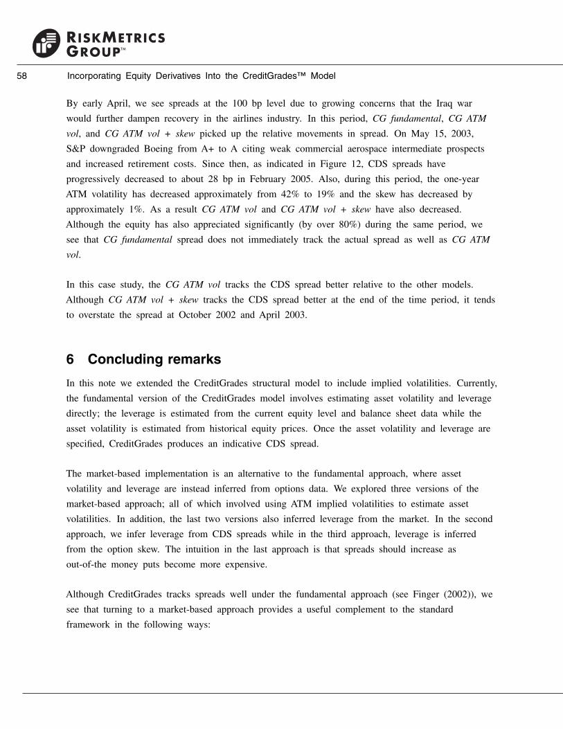
58 Incorporating Equity Derivatives Into the CreditGrades™ Model
By early April, we see spreads at the 100 bp level due to growing concerns that the Iraq war
would further dampen recovery in the airlines industry. In this period, CG fundamental, CG ATM
vol, and CG ATM vol + skew picked up the relative movements in spread. On May 15, 2003,
S&P downgraded Boeing from A+ to A citing weak commercial aerospace intermediate prospects
and increased retirement costs. Since then, as indicated in Figure 12, CDS spreads have
progressively decreased to about 28 bp in February 2005. Also, during this period, the one-year
ATM volatility has decreased approximately from 42% to 19% and the skew has decreased by
approximately 1%. As a result CG ATM vol and CG ATM vol + skew have also decreased.
Although the equity has also appreciated significantly (by over 80%) during the same period, we
see that CG fundamental spread does not immediately track the actual spread as well as CG ATM
vol.
In this case study, the CG ATM vol tracks the CDS spread better relative to the other models.
Although CG ATM vol + skew tracks the CDS spread better at the end of the time period, it tends
to overstate the spread at October 2002 and April 2003.
6 Concluding remarks
In this note we extended the CreditGrades structural model to include implied volatilities. Currently,
the fundamental version of the CreditGrades model involves estimating asset volatility and leverage
directly; the leverage is estimated from the current equity level and balance sheet data while the
asset volatility is estimated from historical equity prices. Once the asset volatility and leverage are
specified, CreditGrades produces an indicative CDS spread.
The market-based implementation is an alternative to the fundamental approach, where asset
volatility and leverage are instead inferred from options data. We explored three versions of the
market-based approach; all of which involved using ATM implied volatilities to estimate asset
volatilities. In addition, the last two versions also inferred leverage from the market. In the second
approach, we infer leverage from CDS spreads while in the third approach, leverage is inferred
from the option skew. The intuition in the last approach is that spreads should increase as
out-of-the money puts become more expensive.
Although CreditGrades tracks spreads well under the fundamental approach (see Finger (2002)), we
see that turning to a market-based approach provides a useful complement to the standard
framework in the following ways:

Concluding remarks 59
• Credit warning signal: Using implied volatilities, (which albeit produce more volatile credit
signals), can provide more timely signals than the fundamental approach. Intuitively, we expect
that the dynamics of equity options should help with forecasts of the spread, especially during a
crisis. During a credit crisis we expect implied volatilities to spike. This intuition was confirmed
as we examined our test cases in Section 5. Secondly, market-based approaches are useful when
a company’s true leverage is difficult to estimate. Instead of estimating leverage from balance
sheet information, it can be estimated by observing historical CDS quotes (for liquid names), or
equity skews. This is useful if we are interested in relative ranking across different names.
• Trading: By utilizing implied volatilities and adjusting leverage (when a company’s true leverage
is difficult to estimate), the CreditGrades model provides better relative pricing than the
fundamental approach. The extended CreditGrades framework can aid in detecting mispricing
between credit and equity options since it provides a link on trades based on credit, equity, and
option positions.
• Vega risk for VaR: Since we can link implied volatilities to spreads, we may extend the ideas
of Mina and Ta (2002), to capture spread volatility. Spread risk volatility can be decomposed,
not only to a component linked to equity prices, but also to a component driven by equity
option volatility.
References• Derman, E., Iraj, K., and Zou, J.Z (1995). The local volatility surface. Unlocking the
information in index option prices, Quantitative Research Notes, Goldman Sachs.
• Finger, C. (ed.) (2002). CreditGradesTM Technical Document, RiskMetrics Group.
• Finger, C., and Stamicar, R. (2005). Better ingredients, RiskMetrics Research Monthly, April
2005.
• Finkelstein, V. (2001). Assessing default probabilities from equity markets, Presentation, Credit
Risk Summit, New York.
• Hull, J., Nelken, I., and White, A. (2005). Merton’s model, credit risk and volatility skews,
Journal of Credit Risk, 1(1): 3–28.
• John, F. (1995). Partial Differential Equations, Springer, 4th edition.
• Merton, R. (1974). On the pricing of corporate debt: the risk structure of interest rates, Journal
of Finance, 29(2): 449–470.

60 Incorporating Equity Derivatives Into the CreditGrades™ Model
• Mina, J., and Ta, T. (2002). Estimating issuer-specific risk for corporate bonds, RiskMetrics
Journal, 3(1): 7–26.
• Shreve, S. (2004). Stochastic Calculus for Finance II, Continuous-Time Models, Springer Finance,
2004.
A Derivation of CreditGrades put value
The European put problem is
∂P
∂t+ 1
2σ 2(S + Bert )2 ∂2P
∂S2+ rS
∂P
∂S− rP = 0, S > 0
P(S, T ) = max(X − S, 0),
P (0, t) = Xe−r(T −t),
where X is the strike price and T is the maturity of the option. Applying the following
transformations
z = log
(S
Bert+ 1
),
τ = 12σ 2(T − t),
leads to an initial-boundary value problem in the quarter plane
uτ = uzz, z > 0, τ > 0
u(z, 0) = e−z/2 max[X + BerT (1 − ez), 0
],
u(0, τ ) = Xeτ/4,
(A.1)
where P(S, t) = e−(2τr)/σ 2+z/2−τ/4u(z, τ ). Using Green’s functions, one can solve (A.1) to obtain the
following solution for the European put
u(z, τ ) =∫ ∞
0�(z, τ ; ξ, 0)u(ξ, 0) dξ +
∫ τ
0u(0, s)�ξ (z, τ ; 0, s) ds,
where the Green’s function �(z, τ ; ξ, s) is given by
�(z, τ ; ξ, s) = G(z, τ ; ξ, s) − G(z, τ ; −ξ, s),
G(z, τ ; ξ, s) = 1√4π(τ − s)
e− (z−ξ)2
4(τ−s) ,

Derivation of CreditGrades put value 61
Re-writing in terms of the original variables and standard normal cumulative distributions gives
P(S, t, B) = Xe−r(T −t)�(a1, a2) − S�(a5) + I (B, σ, S, X),
where
I (B, σ, S, X) = −Xe−r(T −t) [�(a3, a4)] + S [1 − �(a4)]
+Bert [�(a2) − �(a4) − �(a5) + �(a6)] − S
BXe−rT [�(a3, a4)]
+2Xez/2−r(T −t)
∫ ∞
z/√
2τ
1√2π
e−s2/2e−z2/(8s2) ds,
�(x, y) = 1√2π
∫ y
x
e−s2/2 ds,
�(y) = �(−∞, y).
The limits for integration are
a1 = −ση + 12σ 2(T − t)
σ√
T − t,
a2 = −σ(η − ηX) − 12σ 2(T − t)
σ√
T − t,
a3 = ση + 12σ 2(T − t)
σ√
T − t,
a4 = σ(ηX + η) + 12σ 2(T − t)
σ√
T − t,
a5 = −σ(η − ηX) + 12σ 2(T − t)
σ√
T − t,
a6 = σ(ηX + η) − 12σ 2(T − t)
σ√
T − t.
The distance to default parameters are
η = 1
σlog
(1 + S
Bert
),
ηX = 1
σlog
(1 + X
BerT
).

62 Incorporating Equity Derivatives Into the CreditGrades™ Model
B Risk-neutral violation of the equity process
In this appendix, we calculate the amount of risk-neutral violation in the equity process.18 Recall
that the discounted asset process, where the asset process is given by Equation (4), is a martingale
whereas the discounted equity process is not. Although one could add a drift adjustment to make
the equity process risk-neutral, we have instead chosen the asset process to grow at the risk-free
rate in order to preserve the survival probabilities given by Equation (7).
In order to compute the amount of risk-neutral violation in equity, we will need the following
result from the reflection principle. Suppose Wt is a Brownian motion with drift, i.e., Wt = Wt + θt
where Wt is a standard Brownian motion and θ is a constant. Let IP and IP be the associated
measures corresponding to Wt and Wt . Define the running minimum process up to time t as
mWt= min0≤s≤t Ws . The joint density of Wt and mWt
under IP is given by19
g(w, m; t) = 2(w−2m)
t√
2πte− (2m−w)2
2t eθw−θ2t/2, w > m, m < 0.
The joint density function above can now be used to compute the risk-neutral violation in S.
Define the discounted stock and asset processes as St = e−rtSt and Vt = e−rtVt , respectively. In
addition we define the non-absorbing version for the equity and discounted equity processes as Xt
and Xt , respectively. The expected discounted equity process is given by
Y0 = E0(St ) = E0(Xt · I{mXt
>0}), (B.1)
where E0 is the time zero expectation operator under IP and I is the indicator function.
If St was a martingale then Y0 would be equal to S0 = S0. Expanding Equation (B.1) gives
Y0 = E0(Vt · I{mVt
>B}) − BE0(I{mVt
>B}). (B.2)
The second term is simply the product of B and the survival probability F(t) given by Equation
(7). We now evaluate the first term in (B.2) by utilizing the density function g above with
18The authors would like to thank an anonymous referee for pointing this out.19See Shreve (2004).

Risk-neutral violation of the equity process 63
θ = −σ/2 to obtain the following integral
E0(Vt · I{mVt
>B}) = E0(V0eσWt · I{m
Vt>B})
=∫ ∞
C
∫ w
C
V0eσw 2(w−2m)
t√
2πte− (2m−w)2
2t eθw−θ2t/2dm dw
=∫ ∞
C
V0eσw 1√
2πteθw−θ2t/2{e−w2/(2t) − e−(2C−w)2/(2t)} dw,
where C = 1σ
log(B/(B + S0)). Completing the squares in the integrals above and writing in terms
of cumulative normal distributions gives the final result
Y0 = S0 + B
[�
(−C + tσ/2√t
)− �
(−C − tσ/2√t
)].
Note that as B → 0, we obtain that Y0 → S0.
Finally, we present a table listing some examples of the risk-neutral violation. The initial asset
value has been normalized to one. We report the relative error, that is, (S0 − Y0)/Y0. We see that
for a given asset volatility, the relative error increases as the barrier increases (or equivalently, as
equity approaches zero). Further, for parameter levels typical of investment grade credits, we see
that the violation is negligible.
Table B.1
Risk-neutral violation (as relative error in %) in the equity process (V0 = 1, t = 1)
B
σ (%) 0.2 0.4 0.6 0.8
20 0.00 0.00 0.46 14.63
40 0.00 0.79 9.61 35.23
60 0.18 4.83 19.93 46.87

64 Incorporating Equity Derivatives Into the CreditGrades™ Model

65
Adaptations of Monte Carlo SimulationTechniques to American Option Pricing
Serena A. Agoro-MenyangRiskMetrics Group
This article is a review of adaptations of the Monte Carlo simulation methodology to Americanoptions valuation. In examining this topic, we discuss why other numerical methods, such asmultinomial lattice and finite-difference methodologies, are often inadequate for the valuation ofcomplex American options. We then describe three classes of adaptations of the Monte Carlosimulation approach for American options pricing—the regression-based method, the stochasticmesh method, and state-space partitioning method—which are designed to address thedeficiencies of other numerical methods in pricing American options. As part of our survey, wecontrast these three approaches.
1 Introduction
The Monte Carlo simulation methodology is a robust, indispensable tool in derivative security
pricing, for it can be employed in those cases where numerical methods are necessary because
closed-form valuation formulas are not available or not sufficiently accurate. Monte Carlo
simulation is not the only alternative in such cases—there are certainly competing, venerable
methodologies such as binomial/multinomial lattice and finite difference-based methodologies.
However, a general disadvantage with the lattice and finite difference methodologies is that the
computational burden associated with them can grow exponentially with several fairly commonly
observed sources of complexity in derivatives valuation. These sources of complexity are as
follows:
a. Multiplicity of state variables. The number of computations required under lattice and finite
difference methods (as captured by the number of nodes both approaches) can grow
exponentially as the number of sources of systemic risk affecting the pricing of derivatives
securities increase.

66 Adaptations of Monte Carlo Simulation Techniques to American Option Pricing
b. Path Dependency. Typically, reasonably accurate valuation of path-dependent derivatives requires
an exponential increase in lattice or grid density. Often this increase in grid density occurs in
association with the introduction of new state variables to facilitate valuation in the presence of
path dependency.
c. High Resolution Time Grid/Multiplicity of Exercise Opportunities. To evaluate some derivative
instruments with acceptable accuracy, it is necessary to employ time steps that are small relative
to the time to maturity of the instrument. Examples of such instruments include derivatives for
which the number of exercise opportunities is large relative to the lifespan of the instrument.
Unfortunately, the increase in the number of grid points in a lattice or finite difference mesh will
ordinarily increase exponentially with the increase in the number of time steps.
The exponential growth in computational burden exhibited by lattice and finite difference
approaches renders them intractable in the presence of the complications just described. In
contrast, the number of computations required under a Monte Carlo approach usually grows only
linearly or quadratically in the presence of such complexities, not exponentially, which implies that
the Monte Carlo approach is more computationally efficient where these complicating factors are
present.
Despite the apparent robustness and flexibility of the Monte Carlo simulation methodology, this
approach to derivatives valuation does have one serious deficiency—the apparent incompatibility of
the Monte Carlo simulation methodology with American option valuation.1 Valuation of American
options through Monte Carlo simulation is problematic because valuation of such instruments
effectively requires solving an embedded optimization problem; this can be viewed as an optimal
stopping problem—determining the optimal time to exercise the option (that is, to “stop” the
existence of the option) through identification of the optimal exercise boundary. Monte Carlo
simulation techniques are not naturally adapted to solving such an embedded optimization problem.
The reason is that Monte Carlo techniques are fundamentally forward recursive algorithms, in that
the simulated variables are projected forward through time. However, a highly effective way to
value American and Bermudan derivatives is through backward induction because by maturity of
the derivative, the maximum amount of information about the optimal exercise strategy is revealed.
Backward induction algorithms (such as lattice and finite difference-based algorithms) capture this
information and thus can be used to value American options—if they are free of the complexity
1Throughout this survey, we will not distinguish between derivatives with theoretically continuous exercise opportunities prior to expiration(American options) and options with a finite number of exercise opportunities prior to expiration (Bermudan options). We will use the term“American” to refer to both types of derivatives.

A Simplifying Analogy To The Binomial Lattice Approach 67
described earlier (multiplicity of state variables, path dependency, and multiplicity of exercise
opportunities). Unfortunately, capturing this information about optimal exercise policies in the
context of a forward induction algorithm such as Monte Carlo simulation is a challenge.
Nonetheless, there has been considerable research focused upon meeting that challenge by finding
ways to adapt Monte Carlo algorithms to price financial instruments with embedded American
options, given growth in the variety of American options which have features that make valuation
by lattice and finite difference approaches impractical. The purpose of this article is to provide a
survey of the research concerning Monte Carlo-simulation algorithms for American option pricing.
2 A Simplifying Analogy To The BinomialLattice Approach
Most of the adaptations of Monte Carlo simulation technique to American option pricing use
techniques that have analogs to lattice-based approaches. Consequently, it is useful to review the
mechanics of one of the simpler lattice-based approaches to pricing American options—the binomial
lattice approach. In the binomial lattice approach, the price of the underlying asset is modeled as
having a binomial distribution with a probability of an “up” move in the price of the underlying
asset equal to p. We will assume that the cash flows of the American option can be replicated
through investment in correct combinations of “primitive” (that is, “cash” or “non-derivative”)
securities. With this assumption, by standard no-arbitrage pricing arguments, the price of the
American derivative can be computed as the discounted expected value of the American option,
where the expectation is taken with respect to the binomial distribution. In the no-arbitrage pricing
framework, the expectation is computed under the presumption that p represents a risk-neutral
probability; recall that the risk-neutral probability density is the probability density that would
describe asset price behavior if investors were indifferent to risk or “risk-neutral”.
In discussing the binomial lattice approach, it is helpful to keep in mind the pictorial representation
of the underlying price process shown in Figure 1.

68 Adaptations of Monte Carlo Simulation Techniques to American Option Pricing
Figure 1
Binomial lattice approachS 23
S 12
S 01 S 22
S 11
S 21
p
1-p
1-p
p
p
1-pt*= 0n=1
t* =1n =2
t =1n =1
t* =2=Tn =3
t* =2=Tn =2
t* =2=Tn =1
2.1 Notation
In describing the binomial pricing algorithm, the following notation will be used:
T is the date on which the American option expires
t∗ is a discrete time index where t∗ = 0, 1, 2, . . . T , and 0 is the date for which we want to
estimate the value of the American option.
N(t∗) is the number of nodes in the binomial lattice for date t∗ in the binomial lattice
n is the discrete node index for a given time t∗; n = 1, 2, . . . N(t∗).
St∗,n is the value of the underlying asset at time t∗ at node (or “state”) n.
Vt∗,n(St∗,n) is the value of the American option at time t∗ at node n.
V it∗,n(St∗,n) is the intrinsic value of the American option at time t∗ at node n.
V ht∗,n(St∗,n) is the value of the option at time t∗ at node n if the derivative is not exercised. This
is also referred to as the continuation value of the option
rf,t∗ is the continuously compounded risk-free rate of interest over the time interval from t∗ to
t∗ + 1

A Simplifying Analogy To The Binomial Lattice Approach 69
ru,t∗ is the continuously compounded rate of return on the underlying asset in an up move under
the risk-neutral probabilities (such that St∗+1,n = eru,t∗ St∗,n.)
rd,t∗ is the continuously compounded rate of return on the underlying asset in a down move under
the risk-neutral probabilities (such that St∗+1,n = erd,t∗ St∗,n.)
E[·|·] is the conditional expectation operator. For instance, the expected value of y given x (where
y and x are two arbitrary random variables) will be denoted as E[y|x]. We will use the
expression E[·], such as E[x], to denote the unconditional expectation of x.
ˆ is used to denote the estimate of a quantity. For instance, V ht∗,n(St∗,n) represents the estimate of
V ht∗,n(St∗,n).
2.2 Algorithm
The binomial pricing algorithm can be described as follows:
1. Set up the initial lattice for the values of the underlying asset. Note that due to the way the
lattice is structured, if the current value of the underlying asset is St∗,n∗ (where n∗ is one of the
values in the range [1...N(t∗)]), then the price at the next date (time t∗ + 1) in an up move is
St∗+1,n∗+1, and the price of the underlying at the next date in a down move is St∗+1,n∗ . The
value S0,1 is the starting value for the underlying asset and is based on data as of the pricing
date.
2. For all nodes at time T , set the value of the American derivative at time T equal to the
intrinsic value of the derivative at time T .
3. For all times T − 1 to 0, repeat the following subsequence at each node n:
3a. Compute the value of the derivative at node (t∗, n), if it is held and not exercised, as the
probability of an up move multiplied by the discounted value of the derivative at time t∗ + 1 in
an up move plus the probability of a down move multiplied by the discounted value of the
derivative at time t∗ + 1 in a down move. Mathematically, this can be expressed as
V ht∗,n(St∗,n) = E[e−rf,t∗ Vt∗+1(St∗+1)|St∗,n]
= pe−rf,t∗ Vt∗+1,n+1(St∗+1,n+1) + (1 − p)e−rf,t∗ Vt∗+1,n(St∗+1,n)
3b. If the exercise value of the option is worth more than its expected value, then assume the
option is exercised by setting Vt∗,n(St∗,n) equal to V it∗,n(St∗,n). Otherwise, assume the option is

70 Adaptations of Monte Carlo Simulation Techniques to American Option Pricing
held, not exercised, which would imply that Vt∗,n(St∗,n) = V ht∗,n(St∗,n). Mathematically, this can
be represented as:
Vt∗,n(St∗,n) = max(V it∗,n(St∗,n), V
ht∗,n(St∗,n))
A key insight in the binomial lattice approach is that at Step 3a, the derivative holder computes the
conditional expected value of the derivative conditional upon being at a particular node (that is,
conditional upon St∗,n). Then, in Step 3b, the derivative holder uses this conditional expected
value to decide whether to exercise the option or continue holding it.
The adaptations of the Monte Carlo simulation approaches to American option valuation build upon
this insight, for they feature variations on the backward induction logic utilized in the binomial
lattice approach. Where they differ conceptually from the backward induction process contained in
the binomial approach is in:
• The depiction of the price path of the underlying asset. The Monte Carlo approaches to
American derivative valuation use independent Monte Carlo simulations for the St∗,n paths,
where the simulated paths typically represent draws from a continuous probability density—as
opposed to draws from a discrete distribution such as the binomial distribution.
• The method which is used to compute the conditional expectations at Step 3a. The methodology
employed at 3a not only distinguishes the Monte Carlo approaches from the lattice approach but
also from each other.
The Monte Carlo simulation approaches to American option valuation also differ in complexity and
magnitude of computational requirements. The primary Monte Carlo approaches we will examine
are:
• Regression-Based
• Stochastic Mesh
• State-Space Partition
We will focus upon these three classes of approaches because they are among the most robust to
the sources of complexity in American options pricing. However, this list is not exhaustive. For
broader surveys of Monte Carlo simulation approaches to American derivatives valuation, we refer

Regression-Based Monte Carlo Simulation Method 71
the reader to chapter 8 of Glasserman (2004) and to Boyle, Broadie, and Glasserman (1997). The
latter work is particularly useful for reviews of some of the earlier Monte Carlo simulation
methodologies.
3 Regression-Based Monte Carlo SimulationMethod
Examples of research presenting regression-based Monte Carlo simulation methods for valuation of
American options include Carriere (1996), Carriere (undated), Tsitsiklis and VanRoy (1999),
Longstaff and Schwartz (2001), and Tsitsiklis and VanRoy (2001). We list the generic steps of the
regression-based Monte Carlo simulation method, structuring them in such a fashion so as to
accentuate the analogy between the regression-based Monte Carlo method and the binomial lattice
methodology:
3.1 Notation
T is the date on which the American option expires.
t is a discrete index of the exercise dates where t = 0, 1, 2, . . . T , and 0 is the date for which we
want to estimate the value of the American option. If we wish to exclude the possibility of
immediate exercise of the option (that is, to exclude the possibility of exercising the option at
date 0), we can assume that the value of immediate exercise of the option to be 0.)
N is the total number of Monte Carlo simulations or scenarios.
n is the discrete index for the simulations; n = 1, 2, . . . N .
d is the number of asset prices underlying the American option.
St,n is the value of the underlying asset at time t at node (or “state”) n if d = 1. However, in the
case the American option payoff is a function of the price of more than one underlying asset, d
will be greater than one and St,n will represent a vector of asset prices. Mathematically, this is
represented by the expression St,n ∈ �d . A simple example is that of an American call option
on the spread between two stocks. Here, d = 2, and for a given Monte Carlo simulation n and
time t , St,n = [St,n,1St,n,2
] where St,n,1 is the price per share of the first stock at time t in simulation
n and St,n,2 is the price per share of the second stock at time t in simulation n.
S0 is the value of the underlying at time 0. This is one asset if S0 is univariate and a set of
assets if S0 is multivariate.

72 Adaptations of Monte Carlo Simulation Techniques to American Option Pricing
Figure 2
Regression-based Monte Carlo approachS 1,N S 2,N S T,N
S 1,N -1 S 2,N -1 S T,N -1
S 0,1 S 1,3 S 2,3 S T ,3
S 1,2 S 2,2 S T ,2
S 1,1 S 2,1 S T ,1
t =1n =N
t =1n =N-1
t =1n =3
t =1n =2
t =1n =1
t =2n =N
t =2n =N-1
t =2n =3
t =2n =2
t =2n =1
t =Tn =N
t =Tn =N -1
t =Tn =3
t=Tn =2
t=Tn =1
Vt,n(St,n) is the value of the American option at time t at node n.
V0 is the value of the American option at time 0.
V it,n(St,n) is the intrinsic value of the American or Bermudan option
V ht,n(St,n) is the value of the derivative at time t at node n is the derivative is not exercised
rf,t is the continuously compounded risk-free rate of interest over the time interval from t to t + 1
ˆ is used to denote the estimate of a quantity. For instance, V ht,n(St,n) represents the estimate of
V ht,n(St,n).
A schematic diagram for the regression-based Monte Carlo method is provided in Figure 2.
3.2 Algorithm
1. Generate St,n through Monte Carlo simulation using the risk-neutral density associated with the
underlying asset price (or prices, if St,n is multivariate).
2. At the time T , compute the terminal derivative values V iT ,n(ST,n) for each n, n = 1 . . . N .

Regression-Based Monte Carlo Simulation Method 73
3. For all t , t = T − 1 . . . 1, repeat the following backward induction steps:
3a. compute the value of the derivative at node n, t if it is held (instead of exercised) as
V ht,n(St,n) = E[e−rf,t Vt+1(St+1)|St,n],
where E[e−rf,t Vt+1(St+1)|St,n] is the estimate of E[e−rf,t Vt+1(St+1)|St,n] and is computed via
regression of e−rf,t Vt+1,n(St+1,n) on either St,n or a function of St,n. Note that the regression at
Step 3a is cross-sectional in that it is run across the scenarios (as enumerated by n). The
dependent variable is always e−rf,t Vt+1,n(St+1,n), but the form of the regression and of the
regressors (that is, the independent variables) can differ across implementations of the
regression-based Monte Carlo method.
3b. If the exercise value of the option is worth more than its expected value, then assume the
option is exercised and set Vt,n(St,n) equal to V it,n(St,n). Otherwise, assume the option is held,
not exercised, which would imply that Vt,n(St,n) = V ht,n(St,n). Mathematically, this can be
represented as:
Vt,n(St,n) = max(V it,n(St,n), V
ht,n(St,n)).
4. Compute the Monte Carlo estimate of the value of the American option as
V0 = 1
N
N∑n=1
e−rf,0 V1,n(S1,n).
3.3 Remarks
1. Past research has featured different formulations of the regression at Step 3a. Some examples
are as follows:
(a) ordinary least squares regression where St,n is a univariate regressor (that is, d = 1).
(b) ordinary least squares regression where the regressors are deterministic linear and nonlinear
transformations of either a univariate or multivariate St,n. For example, Andersen and Broadie
(2001) illustrate the regression-based Monte Carlo simulation method by computing the value of
an American call on the maximum of two stocks. Here, denote the values of the two stocks
St,n,1 and St,n,2. In their application, Andersen and Broadie (2001) use a variety of linear and
nonlinear combinations of St,n,1 and St,n,2 as independent variables in the regression used to
estimate E[Vt+1(St+1)|St,n]. Combinations include St,n,1, St,n,2, St,n,1 · St,n,2, and BS(St,n,1,St,n,2),

74 Adaptations of Monte Carlo Simulation Techniques to American Option Pricing
where BS(St,n,1,St,n,2) is the value according to the Black-Scholes formula for a European max
call option on St,n,1, and St,n,2.
(c) nonparametric regression with St,n as the regressor (Carriere (1996)).
2. In most regression applications and, in particular, in the examples mentioned in Remark 1, the
estimate of the regression function E[e−rf,t Vt+1(St+1)|St,n] is a linear weighted average of the
dependent variable, where the weights are functions of the regressors (either St,n or functions of
the elements of St,n).
3. A particular advantage of the regression-based Monte Carlo simulation methodology is that the
computational requirements associated with it are generally lower compared to competing
approaches. As stated in the previous remark, the estimate of E[e−rf,t Vt+1(St+1)|St,n] is a
weighted average of the e−rf,t Vt+1,n(St+1) values. For most common regression methodologies, if
N Monte Carlo simulations are executed, then there are N nodes at each time step and the
number of weights to be computed at each time step is ordinarily equal to the number of
regressors times N . Thus, the computational effort entailed in the regression-based Monte Carlo
simulation approach is linear in the number of simulations.
4 Stochastic Mesh Method
The stochastic mesh method was introduced by Broadie and Glasserman (1997); Avramidis and
Matzinger (2002) provide additional convergence results for this approach. In the most basic
formulation of this method, the overall structure of the stochastic mesh Monte Carlo simulation
algorithm is identical to the regression-based Monte Carlo simulation algorithm and will not be
restated here. In particular, the St,n are generated through Monte Carlo simulation as they are in
the regression approach. However, where it does differ significantly from the regression-based
method is in how the estimate of the continuation value is computed, and in the conditioning
information employed in computing the continuation value. In order to facilitate the examination
of how the continuation value is computed, we introduce some new notation to supplement the
notation utilized in the discussion of the regression-based Monte Carlo simulation method; we also
introduce another schematic diagram in Figure 3.

Stochastic Mesh Method 75
Figure 3
Stochastic mesh approach
There are weights at each arrow. Weights from the Nth node: Weights from the 2nd node:at time 2 are labeled: at time 3 are labeled:
S 1,N S 2,N S 3,N S 4,N S T,N
S 1,N -1 S 2,N -1 S 3,N -1 S 4,N -1 S T,N -1
S 0,1 S 1,3 S 2,3 S 3,3 S 4,3 S T ,3
S 1,2 S 2,2 S 3,2 S 4,2 S T ,2
S 1,1 S 2,1 S 3,1 S 4,1 S T ,1W3,2,1
W3,2,2
W3,2,3
W3,2,N -1
W3,2,NW2,N,N-1
W2,N,N
t=1n=N
t=1n=N-1
t=1n=3
t=1n=2
t=1n=1
t=2n=N
t=2n=N-1
t=2n=3
t=2n=2
t=2n=1
t=Tn=N
t=Tn=N -1
t=Tn=3
t=Tn=2
t=Tn=1
t=3n=N
t=3n=N-1
t=3n=3
t=3n=2
t=3n=1
W2,N,3
W2,N,2
W2,N,1
t=4n=N
t=4n=N-1
t=4n=3
t=4n=2
t=4n=1
4.1 Notation
m, n are the indices for the simulations; m = 0, 1, 2, . . . N , n = 0, 1, 2, . . . N
Wt,m,n is the likelihood ratio weight that prevails between node m at time t and node n at time
t + 1.
fSt+1|Stis the probability density for St+1 conditional upon St,n
fSt+1 is the unconditional marginal probability density for St+1
4.2 Remarks
1. How the continuation value is estimated under the stochastic mesh method. As in the regression
method, the estimate of the conditional expected value of the derivative is a weighted average of
the simulated values of the option at time t + 1. The actual functional form of the weights in
the regression-based Monte Carlo approach depends on the form of the actual regression estimate
used. In contrast, the weights in the stochastic mesh method (as presented by Broadie and

76 Adaptations of Monte Carlo Simulation Techniques to American Option Pricing
Glasserman (1997)) are constructed specifically using likelihood ratios—that is ratios of the
probability densities for St+1,n and St,n. Broadie and Glasserman (1997) suggest weights Wt,m,n
that are the ratio of fSt+1,n|St,mto fSt+1,n
or
Wt,m,n = fSt+1,n|St,m
fSt+1,n
, (4.1)
where it is natural to base the weights on conditional distributions fSt+1,n|St,mthat are consistent
with the stochastic process for St .
Under appropriate technical assumptions, Broadie and Glasserman (1997) show that an estimate
of E[e−rf,t Vt+1(St+1)|St+1]—which is the estimate of the continuation value V ht,n(St+1,n)—is given
by the weighted average 1N
∑Nn=1 Wt,m,ne
−rf,t Vt+1(St+1,n). The essence of their argument is that
this weighted average of the e−rf,t Vt+1(St+1) is actually an unweighted average of the values
Wt,m,ne−rf,t Vt+1(St+1,n), and this will converge as N grows large to the unconditional expected
value of Wt,m,ne−rf,t Vt+1(St+1,n)—which is E[Wt,m,ne
−rf,t Vt+1(St+1,n)] with the expectation
computed using fSt+1,n. The choice of Wt,m,n in Equation 4.1 is the one that equates the
unconditional expected value E[Wt,m,ne−rf,t Vt+1(St+1,n)] to the conditional expected value
E[e−rf,t Vt+1(St+1)|St+1]. Then, using this weighted average as an estimate of
E[e−rf,t Vt+1(St+1)|St+1], we can proceed with step 3a and compute V ht,n(St+1,n) as follows:
V ht,n(St,n) = E[e−rf,t Vt+1(St+1)|St+1,n].
Note that we must actually specify fSt+1|Stand fSt+1 . Broadie and Glasserman (1997) caution
that a poor choice of fSt+1 can potentially lead to estimates of V0 that have explosive variance.
However, they argue that one choice of fSt+1 that prevents V0 from having an explosive variance
is to model it as being equal to 1N
∑Nv=1 fSt+1,n|St,v
, which is the average of the conditional
densities fSt+1,m|St,n. Then, the weights take the form
W ∗t,m,n = fSt+1,n|St,m
1N
∑Nv=1 fSt+1,n|St,v
.
Again, Broadie and Glasserman (1997) show that the estimator 1N
∑Nn=1 W ∗
t,m,ne−rf,t Vt+1(St+1,n)
converges to E[e−rf,t Vt+1(St+1)|St+1] under an appropriate set of technical conditions.
2. The conditioning information employed in estimating the continuation value in the stochastic
mesh framework. Unlike most regression-based Monte Carlo simulation methods, the weights in
the stochastic mesh method are a function the future value St+1 (“future” relative to time t) as
well as St . (In contrast, the weights in the weighted averages used to estimate E[Vt+1(St+1)|St ]

State-Space Partitioning 77
are solely functions of past information in the regression-based Monte Carlo simulation
approach.)
3. One disadvantage of the stochastic mesh Monte Carlo simulation method in comparison to the
regression-based method is that it is generally more computationally demanding. Computing the
continuation value V ht,n(St+1) at each node (t, n) requires N weight values, since the weighted
average used to estimate the continuation value, 1N
∑Nn=1 Wt,m,ne
−rf,t Vt+1(St+1,n), contains “N”
terms. If N Monte Carlo simulations are performed, then there are N nodes at each time step
t . Since sums of N weights are being computed at each of N nodes at every time step t , then
the number of weight calculations is approximately T N2. Hence, the computational effort
required in the stochastic mesh method is quadratic in the number of simulations. In contrast,
the computational burden for most regression-based methods is linear in the number of
simulations.
4. Another disadvantage of the stochastic mesh method is its reliance upon an explicit specification
of the conditional density fSt+1,n|St,m. A poor specification of fSt+1,n|St,m
can degrade the quality
of the estimates obtained through this approach. This can be a drawback in cases where
fSt+1,n|St,mis not well understood, or there is little information that can be used to identify or
estimate this density. Worse yet, for a wide variety of problems, fSt+1,n|St,mmay not exist. For
instance, normally fSt+1,n|St,mdoes not exist if the number of sources of systemic risk is fewer
than the dimension d of St—a situation which characterizes the majority of arbitrage-free interest
rate models. Broadie, Glasserman, and Ha (2000) propose solving the non-existence problem by
finding the weights Wt,m,n as solutions to a constrained optimization problem; their suggested
approach has the potential to be computationally time-intensive because the optimization process
may not necessarily converge, may entail difficult computations, could have hard-to-find starting
values, or may converge to an implausible solution.
5 State-Space Partitioning
Examples of this Monte Carlo simulation-based approach to American option pricing include
Barraquand and Martineau (1995) and Bally and Pages (2001). In this methodology, the possible
values that the underlying asset’s price can attain in the future is described by ranges, or bins.
Discussions of this methodology refer to the collection of possible values for the underlying asset
price as the state-space of the price of the underlying asset, and the ranges are referred to as
partitions. Essentially, the conditional expectations that we estimated at Step 3a in the previous
Monte Carlo simulation algorithms are computed, in this approach, using (estimates of) the discrete

78 Adaptations of Monte Carlo Simulation Techniques to American Option Pricing
conditional probabilities that the price of the underlying will move to one bin at time t + 1, given
that it was in some particular bin at time t .
Although the algorithm and notation for the state-space partitioning Monte Carlo simulation
algorithm is similar to the other algorithms previously discussed in this survey, there are some
subtle differences due to prominence of discrete probabilities in this approach. Hence, we will
fully state both the notation and methodology. The notation needed to efficiently describe this
algorithm is as follows (this notation is partly motivated by Barraquand and Martineau (1995) and
Bally and Pages (2001)):
5.1 Notation
T is date on which the American option expires.
t is a discrete index of the exercise dates where t = 0, 1, 2, . . . T , and 0 is the date for which we
want to estimate the value of the American option.
N is the total number of Monte Carlo simulations or scenarios.
n is the index for the simulations; n = 1, 2, . . . N .
d is the number of asset prices underlying the American option.
St,n is the vector of prices for the assets underlying the American option; St,n ∈ �d .
k(t) is the number of partitions at time t of the state-space for the vector of prices for the assets
underlying the American option. The notation k(t) means that the number of partitions—k—is a
function of time.
i∗, k∗ are the indices for the partitions; i∗ = 1, 2, . . . k(t); k∗ = 1, 2, . . . k(t).
P(t) = (P1(t), P2(t), . . . , Pk(t)(t)): is the partition of the state space (at time t) for S(t) ∈ �d into
k(t) partitions. We assume k(0) = 1 and P1(0) = {S0}. As an example, suppose that d = 1,
and we are considering a partition where St is the price per share for a hypothetical stock.
One possible partition of the set of values the stock price could attain (the state space for St ) is
P1(t) = [0, 10),
P2(t) = [10, 20),

State-Space Partitioning 79
P3(t) = [20, 30),
...
P11(t) = [100, ∞)
In this illustration, then, k(t) equals 11. Note that if d > 1, then the partitioning will be
multidimensional.
ci∗,k∗(t) is the count of the number of times the price of the underlying price S(t) moves at time
t + 1 to partition Pk∗(t + 1) after being in partition Pi∗(t) (at time t).
pi∗,k∗(t) = Prob (St+1 ∈ Pk∗(t + 1)|St ∈ Pi∗(t)) is the probability that the value of the underlying
will move to partition Pk∗(t + 1) at time t + 1 given that it is in partition Pi∗(t) at time t .
pi∗,k∗(t) is the estimate of pi∗,k∗(t).
V it,n(St ) is the intrinsic value of the derivative at time t in scenario n corresponding to value of the
underlying St,n.
Vi
t,k∗ is the average value of V it,n(St,n) for those values of St,n within partition Pk∗(t).
A schematic diagram for the state-space partition Monte Carlo simulation method is provided in
Figure 4.
5.2 Algorithm
1. Generate St,n through Monte Carlo simulation using the risk-neutral density associated with the
underlying asset price (or prices, if St,n is multivariate). As part of this step, record the values
ci∗,k∗(t) and compute the estimates of pi∗,k∗(t), which are pi∗,k∗(t), using the relation:
pi∗,k∗(t) = ci∗,k∗(t)∑k(t)k∗=1 ci∗,k∗(t)
Also, as part of this first step, compute V it,i∗—the estimate of E[V i
t (St )|St ∈ Pi∗(t)]. This is the
expected intrinsic value of the American option price at time t , given that the price of the
underlying asset for the American option lies within partition Pi∗(t) at time t .
2. For time T , compute V iT ,i∗ for every partition Pi∗(T ), i∗ = 1, 2, . . . k(T ).

80 Adaptations of Monte Carlo Simulation Techniques to American Option Pricing
Figure 4
State-space partition approach
There are probabilities at each arrow. Probabilities from the k(t)th node Probabilities from the 2nd node:a , b are arbitrary integers for illustration only. at time 2 are labeled: at time 3 are labeled:
S 1,N Pk(1) (1) S 2,NPk( 2) (2) S 3,N
Pk( 3) (3) S 4,NPk( 4) (4) S T,N Pk(T) (T )
S 1,N-1 V 1,k(1) S 2,N- 1 V 2,k( 2) S 3,N-1 V 3,k( 3) S 4,N-1 V 4,k( 4) S T,N-1 V T ,k(T) =
S 1,N-2 S 2,N- 2 S 3,N-2 S 4,N-2 S T,N-2
S 1,n+ 12Pk(1)-a (1) S 2,n+ 12
Pk(2)-a (2) S 3,n+ 12Pk( 3)-a (3) S 4,n+ 12
Pk( 4)-a (4) S T,n+ 12Pk(T)-a (T )
S 1,n+ 11 V 1,k(1)-a S 2,n+ 11 V 2,k(2)-a S 3,n+ 11 V 3,k( 3)-a S 4,n+ 11 V 4,k( 4)-a S T,n+ 11 V T ,k(T)-a =
S 0,1 S 1,n+ 10 S 2,n+ 10 S 3,n+ 10 S 4,n+ 10 S T,n+ 10
S 1,n+ 1Pk(1)-b (1) S 2,n+ 1
Pk(2)-b (2) S 3,n+ 1Pk(3)-b (3) S 4,n+ 1
Pk(4)-b (4) S T,n+ 1Pk(T)-b (T )
S 1,n V 1,k(1)-b S 2,n V 2,k(2)-b S 3,n V 3,k(3)-b S 4,n V 4,k(4)-b S T,n V T ,k(T)-b =
S 1,n- 1 S 2,n- 1 S 3,n- 1 S 4,n- 1 S T,n- 1
S 1,3P1(1) S 2,3
P1 (2) S 3,3P1(3) S 4,3
P1(4) S T ,3P1(T )
S 1,2 V 1,1 S 2,2 V 2,1 S 3,2 V 3,1 S 4,2 V 4,1 S T ,2 V T ,1=
S 1,1 S 2,1 S 3,1 S 4,1 S T ,1
p k (2),k (2)(2)
p k (2),k (2)-a(2)
p k (2),k (2)-b(2)
p k (2),1(2)
p 2,k (3)-a(3)
p 2,k (3)-
p 2,1(3)
p 2,k (3)(3)
iTkTV )(,
iTV 1,
ibTkTV )(,
iaTkTV )(,
3. For all t , t = T − 1 . . . 0, repeat the following backward induction steps:
3a. Compute the value of the derivative at partition Pi∗(t) as
V ht,i∗(St ) = E[e−rf,t Vt+1(St+1)|St,n ∈ Pi∗(t)]
The estimate E[e−rf,t Vt+1(St+1)|St,n ∈ Pi∗(t)] is computed as:
E[e−rf,t Vt+1(St+1)|St,n ∈ Pi∗(t)] =k(t+1)∑k∗=1
pi∗,k∗(t)e−rf,t Vt+1,k∗
3b. Set Vt,i∗(St,n ∈ Pi∗(t)) = max(V it,i∗(St,n ∈ Pi∗(t)), V
ht,i∗(St,n ∈ Pi∗(t))).
5.3 Remarks
1. To obtain good results under this approach, it is important to choose the partitions for the
underlying asset price judiciously. A disadvantage of this methodology is that selecting the
partitions can be difficult. Procedures discussed in Bally and Pages (2001) to identify ideal
partitions are likely to entail considerable computational effort.

Conclusion 81
2. Unfortunately, the number of partitions needed to facilitate accurate pricing tends to grow
exponentially in the dimension d of the underlying asset price vector if we want a partition that
has relatively similar precision in all dimensions. This feature of the methodology suggests that
it is not well suited to American options where the payoff of the derivative is contingent upon
multiple underlying assets.
6 Conclusion
Pricing complex derivatives with American-style exercise opportunities has presented a dilemma in
the asset pricing literature. On the one hand, backward-induction methodologies such as
multinomial and finite-difference lattices are well suited for addressing the optimal stopping problem
inherent in American option valuation. Unfortunately, they may not be computationally feasible for
American options which are complex due to features such as path dependency, multiplicity of state
variables, or the need for a high resolution time index to facilitate valuations. On the other hand,
Monte Carlo simulation methods can be employed for options that have complex features.
However, basic Monte Carlo simulations approaches are generally poorly suited to redress the
optimal stopping problem that American options valuation entails.
Researchers have sought to resolve this dilemma by adapting Monte Carlo simulation methodologies
to American option valuation. We have surveyed three classes of such
adaptations—regression-based, stochastic mesh, and state-space partition Monte Carlo-based
simulation methodologies. All of these have similarly-structured algorithms. They differ primarily
in how conditional expectations for option continuation values are computed and in the information
used in the estimation of conditional expectations. At RiskMetrics Group, we have found the
regression-based methodologies as a class particularly attractive because of this class’ relatively low
computational requirements. In an environment where the volume of instruments to be priced can
be sizable, the fairly conservative computational demand of the regression methodology has a
distinct appeal. Within the regression-based methodological class, we are most strongly interested
at this time in the linear regression approach, in light of our need for robustness, but the actual
specification of the type of regression will probably be a potential area of future research for us.
Nonetheless, given that adapting modifications of Monte Carlo simulation for American options
pricing is an active area of research in general, we anticipate further developments in this arena.

82 Adaptations of Monte Carlo Simulation Techniques to American Option Pricing
References• Andersen, L. and Broadie, M. (2001). A primal−dual simulation algorithm for pricing
multi-dimensional American options. Working Paper, Columbia Business School, New York, NY,
U.S.A.
• Avramidis, A.N., and Matzinger, H. (2002). Convergence of the stochastic mesh estimator for
pricing American options, pp. 1560-1567 in Proceedings of the Winter Simulation Conference,
IEEE Press, New York, NY U.S.A.
• Bally, V. and Pages, G. (2000). A quantization algorithm for solving multi-dimensional optimal
stopping problems, Working Paper, Universite du Maine, France and Universite de Paris XII,
France.
• Barraquand, J. and Martineau, D. (1995). Numerical valuation of high dimensional multivariate
American securities, Journal of Financial and Quantitative Analysis. 30(3): 383-405.
• Broadie, M., and Glasserman, P. (1997). A stochastic mesh method for pricing high-dimensional
American options.
• Broadie, M., Glasserman, P., and Ha, Z. (2000). Pricing American options by simulation using
a stochastic mesh with optimized weights, pp. 32-50 in Probabilistic Constrained Optimization:
Methodology and Applications, S. Uryasev, ed., Kluwer Publishers, Norwell, MA, U.S.A.
• Boyle, P., Broadie, M., and Glasserman, P. (1997). Monte Carlo methods for security pricing,
Journal of Economic Dynamics and Control. 21(8-9): 1267-1321.
• Carriere, J. (1996). Valuation of early−exercise price of options using simulations and
nonparametric regression, Insurance: Mathematics and Economics. 19(1):19-30.
• Carriere, J. (undated). Linear Regression and Standardized Quasi-Monte Carlo For
Approximating Bermudan Options. Working Paper, University of Alberta, Edmonton, Alberta,
Canada.
• Glasserman, P. (2004). Monte Carlo Methods in Financial Engineering, Springer-Verlag, New
York, NY, U.S.A.
• Longstaff, F.A. and Schwartz, E.S. (2001) Valuing American options by simulation: a simple
least-squares approach, Review of Financial Studies. 14(1):113-147.
• Tsitsiklis, J. and Van Roy, B. (1999). Optimal stopping of Markov processes: Hilbert space
theory, approximation algorithms, and an application to pricing high-dimensional financial
derivatives, IEEE Transactions on Automatic Control. 44(10):1840-1851.

Conclusion 83
• Tsitsiklis, J. and Van Roy, B. (2001). Regression methods for pricing complex American−style
options, IEEE Transactions on Neural Networks. 12(4):694-703.

84 Adaptations of Monte Carlo Simulation Techniques to American Option Pricing

www.riskmetrics.com

www.riskmetrics.com

www.riskmetrics.com
New York: 1.212.981.7500 London: 44.(0)20.7842.0260 Tokyo: 81.3.5793.3222 Singapore: [email protected] [email protected] [email protected] [email protected]
RiskMetrics®, HedgePlatform™, CreditMetrics®, RiskServer™, RiskManager™ CreditServer™, CreditManager®, CDOManager™,
DataMetrics™, the RiskMetrics Group Logo, Building Financial Confidence™, RiskMetrics Group Verified™ among others, are trade-
marks and/or service marks owned by or licensed to RiskMetrics Group, Inc. in the United States and other countries. Other brands
or product names are trademarks and/or service marks of their respective owners, should be treated as such, and may be regis-
tered in various jurisdictions. ©Copyright 2005-2006 RiskMetrics Group, Inc. All rights reserved.
RiskMetrics Group is the leading provider of financial analytics and wealth management solutions to financial institutions,
corporations, and central banks worldwide. Hundreds of asset managers, banks, hedge funds, insurance companies,
pension funds, financial advisors, private banks and regulators entrust their risk management needs to our services.
Since the publication of the RiskMetrics Methodology in 1994, RiskMetrics Group research has set the standard for finan-
cial risk management, defining the way risk is measured and managed. The company is headquartered in New York City,
with nine offices worldwide, including London, Tokyo, Singapore and Geneva.