SciPost Phys. 10, 090 (2021)

Josephson oscillations in split one-dimensional Bose gases

Yuri D. van Nieuwkerk1?, Jörg Schmiedmayer2 and Fabian H.L. Essler1

1 Rudolf Peierls Centre for Theoretical Physics, Parks Road, Oxford OX1 3PU2 Vienna Center for Quantum Science and Technology (VCQ), Atominstitut,

TU-Wien, Vienna, Austria

? yuridaniel@gmail.com

Abstract

We consider the non-equilibrium dynamics of a weakly interacting Bose gas tightlyconfined to a highly elongated double well potential. We use a self-consistent time-dependent Hartree–Fock approximation in combination with a projection of the fullthree-dimensional theory to several coupled one-dimensional channels. This allows usto model the time-dependent splitting and phase imprinting of a gas initially confinedto a single quasi one-dimensional potential well and obtain a microscopic description ofthe ensuing damped Josephson oscillations.

Copyright Y. D. v. Nieuwkerk et al.This work is licensed under the Creative CommonsAttribution 4.0 International License.Published by the SciPost Foundation.

Received 19-11-2020Accepted 02-03-2021Published 26-04-2021

Check forupdates

doi:10.21468/SciPostPhys.10.4.090

Contents

1 Introduction 2

2 Time-dependent projection to one-dimensional channels 42.1 Connection to previous literature 62.2 Three channel model 7

3 Measurements and Green’s functions 73.1 Measured operator in time of flight 73.2 Green’s functions of interest 93.3 Experimental data analysis and its relation to Green’s functions 11

4 Hartree–Fock time evolution 124.1 Quality of the SCHF approximation in equilibrium 13

5 Initial state and gas splitting 155.1 Preparation sequence 155.2 Numerical determination of the initial state 16

6 Josephson oscillations 176.1 Experimental parameters 176.2 Assessment of time-dependent truncation errors in a toy model 17

1

SciPost Phys. 10, 090 (2021)

6.3 Characterization of the quantum state after the preparation sequence 186.4 Damping of density-phase oscillations 20

7 Beyond self-consistent Hartree–Fock 23

8 Conclusions 25

A Low energy projection in equilibrium 26

References 28

1 Introduction

Over the last decade and a half quasi-one-dimensional Bose gases have provided a key plat-form for experimental studies of non-equilibrium evolution in isolated one-dimensional many-particle quantum systems, see e.g. [1–16]. This has been an important driver of intense theo-retical activities aimed at understanding non-equilibrium dynamics in paradigmatic models inD = 1, see [17–22] for recent reviews on the subject. A very nice aspect of the cold atom exper-iments is that they provide quantum simulators for low dimensional quantum field theories.For example trapped single-component Bose gases are well described [23] by the Lieb-Linigermodel [24] of a non-relativistic complex scalar field. At low energy densities effective fieldtheory descriptions [25,26] can apply surprisingly well even out of equilibrium [27–30]. Thishas led to novel applications of Luttinger liquid theory and its variants such as the study of fulldistribution functions of quantum observables [31–40]. By modifying the experimental setupsit is in principle possible to engineer particular perturbations to Luttinger liquid theory. Animportant example is given by a system of two tunnel-coupled repulsive Bose gases [41–44],which gives rise to a low-energy description in terms of a Luttinger liquid and a sine-Gordonquantum field theory [45]. The sine-Gordon model is a paradigmatic relativistic quantum fieldtheory that has attracted a huge amount of attention over the last four decades. It has the at-tractive feature that it is exactly solvable [46–48] and has a number of known applications inthe solid state context, see e.g. [26,49–53]. Motivated by the experimental realization via twotunnel-coupled Bose gases the non-equilibrium dynamics of the sine-Gordon model has beenexplored by a number of groups and methods [54–66].

Given that the sine-Gordon description only applies in an appropriate scaling limit a crucialquestion is how close the experiments are to this regime. In equilibrium correlation functionsobtained from time-of-flight measurements of the boson density were found to be in goodagreement with classical field simulations of the sine-Gordon model [11]. In non-equilibriumsituations like the ones studied in Refs. [10, 14, 15] the situation is much less clear. In theseexperiments two elongated Bose gases are prepared in a quantum state characterized by aphase difference between the two gases. A tunnel coupling between the gases is then applied,which induces Josephson-like oscillations of density and phase. These oscillations quicklydamp out and the distribution function of the phase is seen to narrow. Various studies basedon the sine-Gordon model have so far failed to account for these observations [62, 65, 66].In particular, taking into account Gaussian fluctuations on top of the solution of the classicalfield equations in a self-consistent way produces only very weakly damped Josephson-likeoscillations [62,66]. Given this state of affairs it is natural to question whether the experimentsare in the right regime for a sine-Gordon based description to apply. In the experiments one

2

SciPost Phys. 10, 090 (2021)

deals with three dimensional bosons in a time-dependent confining potential. An obviousquestion is how good the low-energy projection to two one-dimensional Bose gases is in theexperimentally relevant parameter regime. Another important issue is that the initial state thatis prepared after splitting the gas and imprinting a phase difference is in fact not known, as thesplitting process has so far only been modelled in a qualitative phenomenological way [67,68],or via methods that rely on a two-mode approximation [69], a classical field approximation[70] or a restriction to the transverse direction only [69]. In order to start addressing thesequestions we return to the drawing board and consider a gas of weakly interacting bosonssubject to a tight harmonic potential in the z-direction, a time-dependent double well potentialV⊥(y, t) in the y-direction and a shallow harmonic potential in the x-direction. This leads tothe Hamiltonian

H3D(t) =

∫

d3 ~r Ψ†( ~r )�

−∇2

2m+

mω2x

2x2 + V⊥(y, t) +

mω2z

2z2

�

Ψ( ~r )

+12

∫

d3 ~r d3 ~r ′ Ψ†( ~r ′)Ψ†( ~r )U( ~r − ~r ′)Ψ( ~r )Ψ( ~r ′) , (1)

where ~r = (x , y, z) is the 3D coordinate and U( ~r ) is the effective interaction potential

U ( ~r ) = 4πas

mδ3 ( ~r ) . (2)

We will always consider elongated gases with ωx � ωz and refer to the x-direction as thelongitudinal, and the remaining coordinates ~r ≡ (y, z) as the transverse directions. In orderto make contact with the experiments of Ref. [14] we use

V⊥(y, t) =m2

�

c1

c2

�2�

y2 − c22

�

I2(t)− I2c

��2

I(t) + Ic+ F(t)y , (3)

with the values c1 = 2π · 2.52 kHz, c2 = 2.17µm and Ic = 0.4. For I(t) = Ic, V⊥ is a quarticpotential with a flat bottom and for I > Ic, it develops a double well structure. The term F(t)yis used to imprint a phase difference between the gases in the two wells (a precise descriptionof what we mean by this is given below). The explicit form of the functions I(t) and F(t) isgiven in Sec. 5.1, cf. Eqs. (54) and (55).

The idea is to use (1) to describe the splitting of the gas, the phase imprinting and finally thesubsequent non-equilibrium dynamics, but to take advantage of the fact that (i) interactionsare weak; (ii) the confinement is tight in the y- and z-directions. The combination of these twoallows us to project the full three-dimensional theory to a small number of one-dimensionalchannels

Hproj(t) =a−1∑

a=0

∫

d x ψ†a(x , t)

�

−1

2m∂ 2

∂ x2+

mω2

2x2 + εa(t)

�

ψa(x , t)

+

∫

d xa−1∑

a,b,c,d=0

Γabcd(t) ψ†a(x , t)ψ†

b(x , t)ψc(x , t)ψd(x , t) . (4)

The resulting Hamiltonian is time-dependent but retardation effects are negligible. Some com-ments on the projection procedure are provided in Appendix A. We stress that as a result ofworking with the instantaneous basis of single-particle eigenstates of −∂ 2

y /2m+ V⊥(y, t) our

effective one-dimensional field operators ψ†a(x , t) have an explicit time dependence. After

working out how to obtain Hproj(t) from (2) we proceed as follows:

3

SciPost Phys. 10, 090 (2021)

1. We treat the interactions in a time-dependent self-consistent Hartree–Fock approxima-tion (SCHFA). As we are dealing with an effective one-dimensional system we do notallow for the formation of long-range order. The resulting approximation is quite differ-ent from Gross-Pitaevskii theory (see e.g. [71–73]). The main attraction of the SCHFAis that it can be implemented straightforwardly, while its main limitation is that it treatsinteraction effects in a rather crude way. However, it is nonetheless expected to providea good description as long as the interaction strength is sufficiently weak and the energydensity in the system is not too low. We first identify a corresponding parameter regimeand then model the Josephson oscillations experiments in this regime.

2. We start with a confining potential that forms a single elongated well and initialize oursystem in a thermal low-temperature state.

3. We evolve the state under a time-dependent transverse potential V⊥(y, t) that models thesplitting and phase imprinting protocols used in the experiments. This provides us with acharacterization of the “initial state” used in the Josephson-like oscillation experiments.

4. Finally we consider the non-equilibrium evolution of the split, phase-imprinted state.We observe damped Josephson-like oscillations.

This paper is organized as follows. In Sec. 2, we describe the low-energy projection usedto arrive at the Hamiltonian (4), and the rationale for considering one-dimensional field op-erators carrying explicit time-dependence. In Sec. 3, we introduce the observables relevantto experiment, and connect them to the Green’s functions of one-dimensional field operatorsthat are computed in this paper. Sec. 4 introduces the self-consistent time-dependent Hartree–Fock approximation, and the resulting nonlinear partial differential equations that govern thetime-evolution of the experimentally relevant Green’s functions. Sec. 5 describes how the ini-tial state of the system is modelled by preparing a gas in a thermal state of a single well andsplitting it by a deformation of the trapping potential. The time-dependent definition of theone-dimensional field operators is shown to be an important tool in enabling this model forthe preparation sequence. In Sec. 6, numerical results are presented for the time-evolutionof experimentally relevant observables after the preparation stage. Density-phase oscillationsare observed to be strongly damped over timescales that are comparable to those seen in theexperiment.

2 Time-dependent projection to one-dimensional channels

We start from the 3D Hamiltonian (1) with δ-interactions (2),

H3D =

∫

d3 ~r Ψ†( ~r )�

Dx + Dy(t) + Dz +2πas

mΨ†( ~r )Ψ( ~r )

�

Ψ( ~r ), (5)

where we have defined Du = −∂ 2u /2m+mω2

uu2/2 for u= x , z, and

Dy(t) = −1

2m∂ 2

∂ y2+ V⊥(y, t) . (6)

The 3D Bose field Ψ( ~r ) satisfies the usual bosonic commutation relations. We use a doublewell potential of the form (3) for V⊥(y, t) throughout this paper, where the phase imprinting isimplemented by the imbalance potential F(t)y . To arrive at an effective 1D model, we expand

4

SciPost Phys. 10, 090 (2021)

the 3D field operator in an instantaneous basis of single-particle eigenstates of the quadraticpart of the Hamiltonian

Ψ( ~r ) =∞∑

a,b,c=0

χa(x)Φb(y, t)Ξc(z)ba,b,c(t) =∞∑

b,c=0

Φb(y, t)Ξc(z)ˆψb,c(x , t) (7)

Here the single-particle eigenstates fulfil

Dxχa(x) =ωx

�

a+12

�

χa(x) ,

Dy(t)Φb(y, t) = εb(t)Φb(y, t) ,

DzΞc(z) =ωz

�

c +12

�

Ξc(z) , (8)

and we have defined canonical 1D Bose field operators by

ˆψb,c(x , t) =∞∑

a=0

χa(x)ba,b,c(t) , [ ˆψb,c(x , t), ˆψ†b′,c′(x

′, t)] = δb,b′δc,c′δ(x − x ′). (9)

At this stage we are dealing with an infinite number of Bose fields. We now exploit the factthat the single-particle eigenvalues ωz(c + 1/2) and εb(t) constitute very large energy scalesfor c ≥ 1 and b ≥ a, and that interactions are weak. This allows us to truncate the expansionof the 3D Bose fields (7) to a small, finite number of channels. The rationale for workingwith explicitly time-dependent single-particle states rather than working in a fixed basis isthat a subset chosen to span the low-energy subspace of the free part of the Hamiltonian (5)at t = 0 will in general only span the low-energy subspace at later times if we include a largenumber of channels. This would make the truncation much less efficient. Let us now give thedetails of the truncation procedure outlined above. If ωz � ωx , we expect the dynamics tobe frozen into the lowest single-particle eigenstates in the z-direction. We can then projectto the corresponding low-energy subspace by truncating the expansion (7) to the c = 0 term.In the y-direction, the double well V⊥(y, t) gives rise to more states in the low-energy sectorthan just the ground state. We therefore need to retain multiple single-particle eigenstatesΦb(y, t). These wave functions are explicitly time-dependent eigenstates of the double welloperator Dy(t) from Eq. (6), with eigenvalues εa(t). If these eigenvalues show a gap aboveenergy εa−1(t) that is large compared to all other energy scales in the problem for all times,the expansion (7) can be truncated at a = a. The resulting projection of the 3D field operatorto the low-energy sector then reads

Ψ( ~r )≈ Ξ0(z)a−1∑

a=0

Φa(y, t)ψa(x , t) , (10)

where we have defined

ψa(x , t)≡ ˆψa,0(x , t) , (11)

which satisfies [ψa(x , t), ψ†b(x′, t)] = δabδ(x − x ′) for all times. When starting from the 3D

Hamiltonian (5), inserting the projected operator (10) and integrating in the y, z-directionsleads to a model for a species of bosons,

H(a)1D (t) =a−1∑

a=0

∫

d x ψ†a(x , t)

�

−1

2m∂ 2

∂ x2+

mω2

2x2 + εa(t)

�

ψa(x , t)

+

∫

d xa−1∑

a,b,c,d=0

Γabcd(t) ψ†a(x , t)ψ†

b(x , t)ψc(x , t)ψd(x , t) , (12)

5

SciPost Phys. 10, 090 (2021)

with coupling constants that are given by overlap tensors

Γabcd(t) = as

√

√2πωz

m

∫

d y Φ∗a(y, t)Φ∗b(y, t)Φc(y, t)Φd(y, t) . (13)

Corrections to (12) will be negligible as long as the following conditions hold:

• Interactions are small. This holds by construction.

• The initial occupation numbers Tr[ρ(0) b†a,b,c(0)ba,b,c(0)], where ρ(0) is the density

matrix at time t = 0, are very small for c > 0 and b ≥ a. We ensure that this is the caseby working with an initial thermal density matrix at a sufficiently low energy densitycompared to εa(t). Experimentally this condition could be fulfilled by making V⊥(y, t)sufficiently tight.

• The transverse potential is changed slowly enough so that Tr[ρ(t) b†a,b,c(t)ba,b,c(t)] re-

main very small for c > 0 and b ≥ a. This provides a (rather obvious) restriction on theexperimental protocol.

In equilibrium it is straightforward to evaluate the corrections to (12) and we outline thenecessary steps in Appendix A. Perturbatively integrating out the high-energy channels abovesome cutoff generates all two, four and six boson interactions between the low-energy channelsallowed by particle conservation. The interactions are very slightly retarded and non-local inspace (the corresponding scales are set by the cut-off energy) but are negligible compared tothe terms retained in (12). An analogous analysis can be in principle be carried out in thetime-dependent situation of interest here, but as we don’t require the corrections we do notfollow this line of enquiry further.

2.1 Connection to previous literature

For time-independent double-well potentials with a very high tunnel-barrier, the lowest twosingle-particle eigenstates Φ0,1(y) are approximately given by symmetric and anti-symmetriccombinations of wave packets gL,R(y) that are localized in the left and right wells

Φ0,1(y) = (gR(y)± gL(y))/p

2 . (14)

We can then define left- and right-localized one-dimensional Bose operators ψL,R ≈ (ψ0±ψ1)×1/p

2. Inserting these definitions into Eq. (4) with a = 2 leads to the model

H1D→ HLL

�

ψL

�

+HLL

�

ψR

�

−ε1 − ε0

2

∫ L

0

d x�

ψ†L(x)ψR(x) + h.c.

�

, (15)

of two Lieb-Liniger Hamiltonians

HLL

�

ψ�

=

∫

d x ψ†(x)

�

−1

2m∂ 2

∂ x2+

mω2

2x2

�

ψ(x) + g

∫

d x ψ†(x)ψ†(x)ψ(x)ψ(x) , (16)

connected by a tunnel-coupling term. The coupling constant of the Lieb-Liniger model is givenby

g=

∫

d x g∗L(x)g∗L(x)gL(x)gL(x) =

∫

d x g∗R(x)g∗R(x)gR(x)gR(x) . (17)

All other overlap tensors involving four combinations of gL,R(x) vanish if the two wells areseparated by a high tunnel barrier, so that the only coupling between the left and right gasesis given by the tunneling term proportional to (ε1− ε0)/2. Eq. (15) is the Hamiltonian that isstudied in most of the literature, following Ref. [45]. In this paper, we will instead focus onthe more general Hamiltonian (12).

6

SciPost Phys. 10, 090 (2021)

2.2 Three channel model

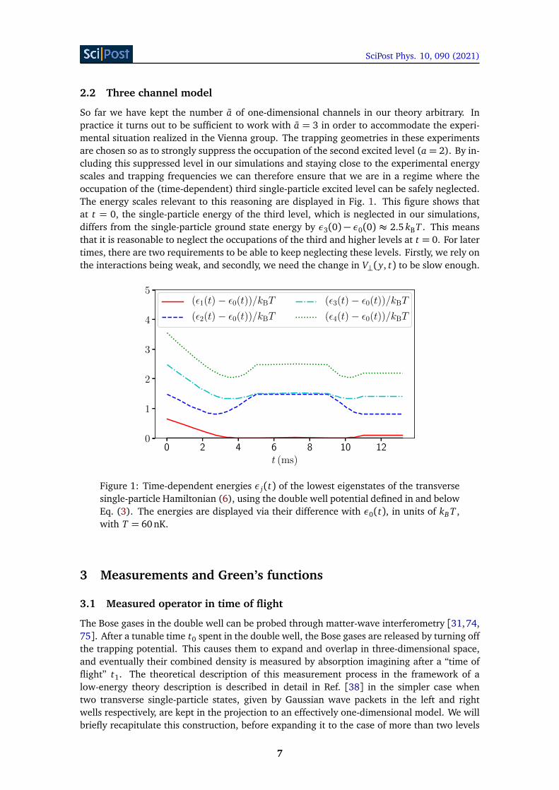
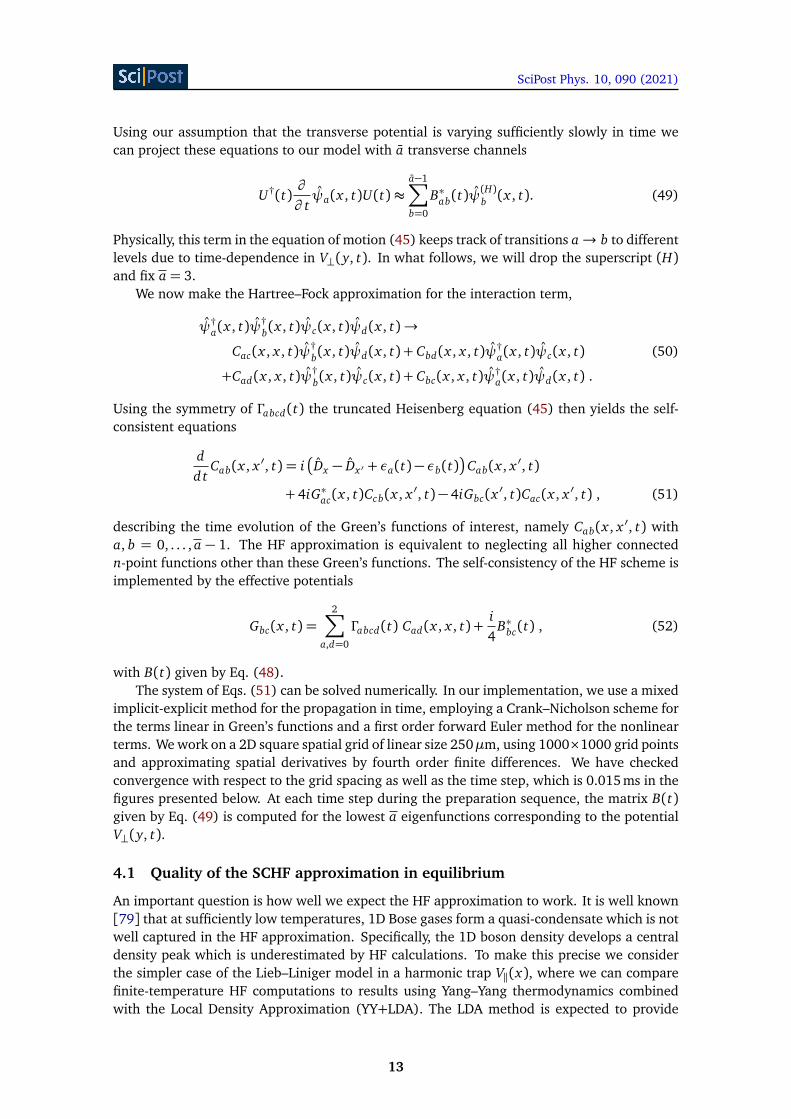
So far we have kept the number a of one-dimensional channels in our theory arbitrary. Inpractice it turns out to be sufficient to work with a = 3 in order to accommodate the experi-mental situation realized in the Vienna group. The trapping geometries in these experimentsare chosen so as to strongly suppress the occupation of the second excited level (a = 2). By in-cluding this suppressed level in our simulations and staying close to the experimental energyscales and trapping frequencies we can therefore ensure that we are in a regime where theoccupation of the (time-dependent) third single-particle excited level can be safely neglected.The energy scales relevant to this reasoning are displayed in Fig. 1. This figure shows thatat t = 0, the single-particle energy of the third level, which is neglected in our simulations,differs from the single-particle ground state energy by ε3(0) − ε0(0) ≈ 2.5 kBT . This meansthat it is reasonable to neglect the occupations of the third and higher levels at t = 0. For latertimes, there are two requirements to be able to keep neglecting these levels. Firstly, we rely onthe interactions being weak, and secondly, we need the change in V⊥(y, t) to be slow enough.

0 2 4 6 8 10 12t (ms)

0

1

2

3

4

5(ε1(t)− ε0(t))/kBT

(ε2(t)− ε0(t))/kBT

(ε3(t)− ε0(t))/kBT

(ε4(t)− ε0(t))/kBT

Figure 1: Time-dependent energies ε j(t) of the lowest eigenstates of the transversesingle-particle Hamiltonian (6), using the double well potential defined in and belowEq. (3). The energies are displayed via their difference with ε0(t), in units of kB T ,with T = 60 nK.

3 Measurements and Green’s functions

3.1 Measured operator in time of flight

The Bose gases in the double well can be probed through matter-wave interferometry [31,74,75]. After a tunable time t0 spent in the double well, the Bose gases are released by turning offthe trapping potential. This causes them to expand and overlap in three-dimensional space,and eventually their combined density is measured by absorption imagining after a “time offlight” t1. The theoretical description of this measurement process in the framework of alow-energy theory description is described in detail in Ref. [38] in the simpler case whentwo transverse single-particle states, given by Gaussian wave packets in the left and rightwells respectively, are kept in the projection to an effectively one-dimensional model. We willbriefly recapitulate this construction, before expanding it to the case of more than two levels

7

SciPost Phys. 10, 090 (2021)

that are not perfectly localized in the wells. The absorption imagining can be thought of as avon-Neumann measurement of the boson density at time t0 + t1

ρtof(r) = Ψ†(r)Ψ(r) . (18)

The density operator is diagonal in the position eigenbasis {|r1, . . . , rN ⟩} which implies thatthe measurement outcomes are particle positions

∑Nj=1δ(r−r j) and the associated probability

distribution is

P(r1, . . . , rN ; t0 + t1) = ⟨r1, . . . , rN |%(t0 + t1)|r1, . . . , rN ⟩ , (19)

where %(t0 + t1) is the density matrix of the system at time t0 + t1. The moments of thisprobability distribution are

Mn(r1, . . . , rn) = Tr�

%(t0 + t1) O†(r1, . . . , rn)O(r1, . . . , rn)�

,

O(r1, . . . , rn) = Ψ(r1) . . . Ψ(rn) . (20)

The density matrix at time t is given by

%(t) = U(t, 0)%(0)U†(t, 0) , U(t, t0) = T exp�

− i

∫ t

t0

d t ′H3D(t′)�

. (21)

In the Heisenberg picture we have

Mn(r1, . . . , rN ) = Tr�

%(0)�

O(H)(r1, . . . , rn, t0 + t1)�†O(H)(r1, . . . , rn, t0 + t1)

�

, (22)

where the Heisenberg-picture field operators are given by

Ψ(H)(r, t) = U†(t, 0)Ψ(H)(r, 0)U(t, 0) . (23)

The approach of Ref. [75] is to relate the quantum state of the system after time-of-flight tothe state at the time of trap release by assuming that interactions are negligible during thetime of flight. This is a reasonable assumption since the gas, which is no longer constrainedand expands in 3D, very quickly becomes highly dilute. The free, transverse expansion is theneffectuated by the evolution operator

U(t1 + t0, t0)≈ e−i t1

�

P2x+P2

y+P2z

�

/2m . (24)

This allows us to relate the Heisenberg picture field operators at times t0 + t1 and t0

Ψ(H)(r, t0 + t1) =

∫

d3r′ G0(r− r′, t1) Ψ(H)(r′, t0) , (25)

where G0(r, t) is the propagator of the non-interacting boson Hamiltonian describing the freeexpansion. Now we exploit the fact that the initial density matrix ρ(0) involves only the low-energy sector, i.e. states in which only very few transverse modes are occupied. This allows usto project the field operators Ψ(H)(r, t0) and concomitantly the operators O(H)(r1, . . . , rn, t0+t1)in the expression (22) for the moments Mn to the low-energy description

Ψ(H)(r, t0)≈ Ξ0(z)∑

a∈S

ga(y, t)ψ(H)a (x , t) , (26)

where S is some set of indices labeling single-particle states ga(y, t) in the transverse direction.The equations of motion of the Heisenberg picture operators ψ(H)a (x , t) are derived below in

8

SciPost Phys. 10, 090 (2021)

section 4. In [38], this set S = {L, R} refers to single-particle states with no explicit time-dependence that are localized in the left and right wells, respectively. In the following we willfocus on the average over many absorption images

M1(r) = Tr�

%(0) ρ(H)tof (r, t0 + t1)�

. (27)

Carrying out the convolutions we obtain

ρ(H)tof (r, t0 + t1)≈ |Ξ0(z, t1)|2

∑

i, j∈S

Ai j(y, t0, t1)

∫

d x ′d x G∗0(x − x ′, t1)G0(x − x , t1)

�

ψ(H)i (x

′, t0)�†ψ(H)j ( x , t0) . (28)

Here we have defined

Ai j(y, t0, t1) = g∗i (y, t0, t1)g j(y, t0, t1), i, j ∈ S ,

g j(y, t0, t1)≡∫

d y ′√

√ m2πi t1

exp�

im

2t1(y − y ′)2

�

g j(y′, t0) , (29)

and an analogous expression is obtained for Ξ0(z). The higher moments Mn>1 can be relatedto expectation values in the low-energy description in the same way.

In many works [44,75] it is assumed that the longitudinal expansion has little effect (eventhough it can be straightforwardly taken into account in a low-energy field theory frameworkin some cases [38]). This assumption is based on the state at the time of trap release: sincethe gas is spatially very constrained in the transverse directions, its momentum distribution inthese directions is much broader than in the longitudinal direction. As a result, the time scalefor expansion in the longitudinal direction far exceeds that for the transverse directions. If thetime of flight t1 is short, this suggests the approximation of neglecting longitudinal expansionaltogether, replacing the free evolution operator (24) by

U(t1 + t0; t0)≈ e−i t1

�

P2y+P2

z

�

/2m . (30)

This results in a simplified expression for the operator ρ(H)tof

ρ(H)tof (r, t1, t0)≈ |Ξ0(z, t1)|2

∑

i, j∈S

Ai j(y, t0, t1)�

ψ(H)i (x , t0)

�†ψ(H)j (x , t0) . (31)

We will use this approximate expression in much of the remainder of this work.

3.2 Green’s functions of interest

In what follows, we will derive equations of motion for the Green’s functions of the 1D Bosefields, defined as

Ci j(x , x ′, t)≡ ⟨ψ†i (x , t)ψ j(x

′, t)⟩ . (32)

Solving these numerically gives us access to the expectation value of ρ(H)tof (r, t0 + t1) as wellas averages of Fourier-transformed quantities like (41). In order to connect to the experimen-tal works [10, 14, 15] we have to account for the fact that the data extracted from absorp-tion imaging has been analyzed in terms of the number/phase representation for an effective

9

SciPost Phys. 10, 090 (2021)

two-channel model. Denoting the corresponding Bose field operators by ψL,R we can defineaverages of the relative density and phase via

ϕ(x , t) = Arg ⟨ψ†L(x , t)ψR(x , t)⟩ ,

n(x , t) = ⟨ψ†L(x , t)ψL(x , t)⟩ − ⟨ψ†

R(x , t)ψR(x , t)⟩ . (33)

In order to connect to these quantities we need to express ψL,R in terms of operators in ourthree-channel model. As interactions are weak this transformation can be taken to be linear.To be specific let us work with an effective three-channel model, i.e. a = 3. We then carry outa change of basis such that

ψα(x , t) =2∑

j=0

c(α)j (t)ψ j(x , t), α= L, R, e. (34)

We have introduced a third, “excited” boson species ψe to be able to span the full space of 3transverse levels. The set of labels used in Eq. (26) thus becomes S = {L, R, e}, so that Eq. (26)is equivalent to Eq. (10) under the identifications

Φ j(y, t) =∑

α=L,R,e

c(α)j (t)gα(y, t), j = 0,1, 2. (35)

The transformation matrices c(α)j (t) are chosen with orthonormal rows and columns, so thatthey translate between the basis of single-particle eigenstates Φ0,1,2(y, t) of the transverse op-erator Dy(t) and another basis that contains left- and right-localized wave functions gL,R(y, t)as well es a third wave function, ge(y, t).

In [38], the wave functions gL,R(y, t) were simply given by (anti)symmetric combinationsof Φ0 and Φ1. However, the presence of the third wave function ge(y, t) now creates ambiguity,meaning that the c(α)j (t) can be defined in multiple ways. We will give two options here.Choice 1: Following Ref. [38], we simply choose

c(L)0 c(R)0 c(e)0

c(L)1 c(R)1 c(e)1

c(L)2 c(R)2 c(e)2

(t) =1p

2

1 1 01 −1 00 0

p2

∀ t . (36)

Choice 2: Since the double well is centered around y = 0, we find the vector c(L)j (t) by

minimizing∫∞

0 d y |gL(y, t)|2 subject to the constraint∑

j |c(L)j (t)|

2 = 1. This fixes gL(y, t)as the single-particle wave function in the space spanned by Φ0,1,2(y, t) with the smallestpossible probability for the particle to be found at y > 0, i.e. in the right well. Mutatismutandis for c(R)j (t). The third vector c(e)j (t) is then defined as the orthogonal complement

of the vectors c(L)j (t) and c(R)j (t). The experimentally relevant parameters for the double wellpotential are given below Eq. (3), with 0.5 ≤ I ≤ 0.6 for the oscillation stage. For most ofthese values choices 1 and 2 lead to very similar values of c( j)j (t) and for I ≥ 0.55, the valuesare practically indistinguishable. We will therefore present results for the much simpler Choice1, and comment on the changes that occur for Choice 2 wherever they are relevant.

Using Choice 1 and Eq. (33), the average relative density and phase (33) are given by

ϕ(x , t)≡ Arg CLR(x , x , t)

= Arg12

�

C00(x , x , t)− C01(x , x , t) + C∗01(x , x , t)− C11(x , x , t)�

, (37)

n(x , t)≡ ⟨n(x , t)⟩= CLL(x , x , t)− CRR(x , x , t) = 2Re C01(x , x) . (38)

10

SciPost Phys. 10, 090 (2021)

Another quantity of experimental interest is the mean interference contrast, which we define as

C(x , t) =2 |CLR(x , x , t)|

|CLL(x , x , t) + CRR(x , x , t)|. (39)

3.3 Experimental data analysis and its relation to Green’s functions

As discussed above the average over many absorption images gives access to

⟨ρ(H)tof (r, t1 + t0)⟩ ≈ |Ξ0(z, t1)|2∑

i, j∈{L,R,e}

Ai j(y, t0, t1)

�

ψ(H)i (x , t0)

�†ψ(H)j (x , t0)

�

(40)

in the three-channel model. We refer to Eq. (28) for the case when longitudinal expansion istaken into account. We will now show that the phase ϕ(x , t0) of interest in Eq. (37) can beextracted from M1(r) by taking a suitable partial Fourier transform

Fq

�

⟨ρ(H)tof (r, t1 + t0)⟩�

=

∫

d y e−iq y⟨ρ(H)tof (r, t1 + t0)⟩ . (41)

In the simpler case of gases whose transverse single-particle states are given by Gaussian wavepackets in the left and right wells respectively the choice q = md/t1, where d is the distancebetween the wells’ minima, gives access to the relative phase, see e.g. Ref. [38].

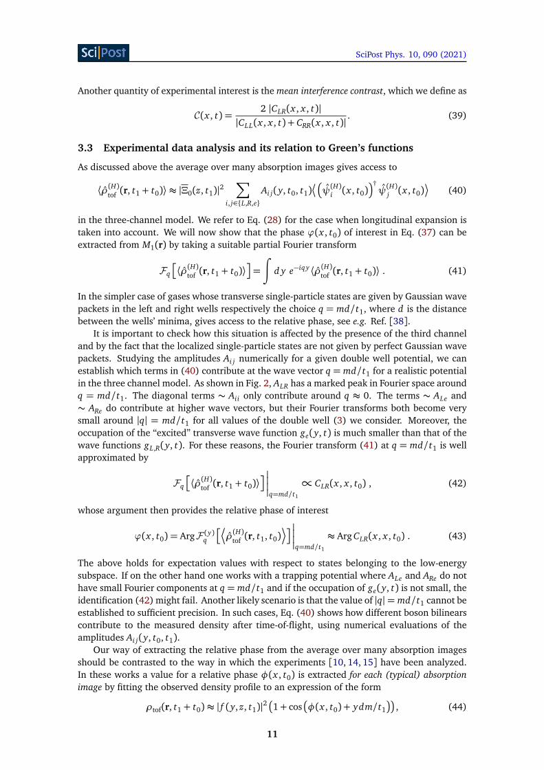
It is important to check how this situation is affected by the presence of the third channeland by the fact that the localized single-particle states are not given by perfect Gaussian wavepackets. Studying the amplitudes Ai j numerically for a given double well potential, we canestablish which terms in (40) contribute at the wave vector q = md/t1 for a realistic potentialin the three channel model. As shown in Fig. 2, ALR has a marked peak in Fourier space aroundq = md/t1. The diagonal terms ∼ Aii only contribute around q ≈ 0. The terms ∼ ALe and∼ ARe do contribute at higher wave vectors, but their Fourier transforms both become verysmall around |q| = md/t1 for all values of the double well (3) we consider. Moreover, theoccupation of the “excited” transverse wave function ge(y, t) is much smaller than that of thewave functions gL,R(y, t). For these reasons, the Fourier transform (41) at q = md/t1 is wellapproximated by

Fq

�

⟨ρ(H)tof (r, t1 + t0)⟩�

�

�

�

�

q=md/t1

∝ CLR(x , x , t0) , (42)

whose argument then provides the relative phase of interest

ϕ(x , t0) = ArgF (y)q

�¬

ρ(H)tof (r, t1, t0)

¶�

�

�

�

�

q=md/t1

≈ Arg CLR(x , x , t0) . (43)

The above holds for expectation values with respect to states belonging to the low-energysubspace. If on the other hand one works with a trapping potential where ALe and ARe do nothave small Fourier components at q = md/t1 and if the occupation of ge(y, t) is not small, theidentification (42) might fail. Another likely scenario is that the value of |q|= md/t1 cannot beestablished to sufficient precision. In such cases, Eq. (40) shows how different boson bilinearscontribute to the measured density after time-of-flight, using numerical evaluations of theamplitudes Ai j(y, t0, t1).

Our way of extracting the relative phase from the average over many absorption imagesshould be contrasted to the way in which the experiments [10, 14, 15] have been analyzed.In these works a value for a relative phase φ(x , t0) is extracted for each (typical) absorptionimage by fitting the observed density profile to an expression of the form

ρtof(r, t1 + t0)≈ | f (y, z, t1)|2 �1+ cos

�

φ(x , t0) + ydm/t1

��

, (44)

11

SciPost Phys. 10, 090 (2021)

1.5 1.0 0.5 0.0 0.5 1.0 1.5q

0.00

0.25

0.50

0.75

1.00

1.25

1.50

1.75

2.00

q()

| q(g*LgR)|

| q(g*Lge)|

| q(g*LgL + g*

RgR)|q = md/t1

Figure 2: Fourier transformed products of single-particle wave functions after time-of-flight g L,R(y, t1) occurring in Eq. (31), for the parameters given below Eq. 3 withI = 0.5. The cross term g∗L(y, t1)gR(y, t1) (green) shows a peak around q = md/t1,whereas g∗L(y, t1)g e(y, t1) (cyan) becomes small there. The same can be said aboutthe other cross terms involving g e. This allows to extract ϕa(x) using Eq. (43).

where f (y, z, t1) is a Gaussian envelope. The data is then analyzed in terms of the averageφ(x , t0) over many shots. An interesting open question is to establish the precise relationbetween φ(x , t0) and ϕ(x , t0) extracted from the average over many images.

4 Hartree–Fock time evolution

Having established how Green’s functions are related to averages over experimental measure-ments, we now consider their time evolution. We do so in the Heisenberg picture, indicatedwith a superscript (H), and consider the equations of motion for the 1D field operators,

idd tψ(H)a (x , t) =

�

ψ(H)a (x , t), H(a,H)1D (t)

�

+ iU†(t)∂

∂ tψa(x , t)U(t) . (45)

Here U(t) is the time-evolution operator

U(t) = T exp�

− i

∫ t

0

d t ′H(a)1D (t′)�

, (46)

and the additional, explicit time-derivative is nonzero due to the time-dependent definitionof ψa(x , t), via the corresponding eigenstates Φa(y, t) of the transverse potential V⊥(y, t). Inorder to work out the last term on the right hand side of (45) we revert to the expansion ofthe Bose field into channels without projection (7)

0=∂ Ψ( ~r )∂ t

=∂

∂ t

∑

b,c

Φb(y, t)Ξc(z)ˆψb,c(x , t). (47)

The orthonormality of the single-particle wave functions then implies that

∂

∂ tˆψbc(x , t) =

∞∑

d=0

B∗cd(t)ˆψcd(x , t), Bab(t) = −

∫

d y Φa(y, t)Φ∗b(y, t) . (48)

12

SciPost Phys. 10, 090 (2021)

Using our assumption that the transverse potential is varying sufficiently slowly in time wecan project these equations to our model with a transverse channels

U†(t)∂

∂ tψa(x , t)U(t)≈

a−1∑

b=0

B∗ab(t)ψ(H)b (x , t). (49)

Physically, this term in the equation of motion (45) keeps track of transitions a→ b to differentlevels due to time-dependence in V⊥(y, t). In what follows, we will drop the superscript (H)and fix a = 3.

We now make the Hartree–Fock approximation for the interaction term,

ψ†a(x , t)ψ†

b(x , t)ψc(x , t)ψd(x , t)→

Cac(x , x , t)ψ†b(x , t)ψd(x , t) + Cbd(x , x , t)ψ†

a(x , t)ψc(x , t) (50)

+Cad(x , x , t)ψ†b(x , t)ψc(x , t) + Cbc(x , x , t)ψ†

a(x , t)ψd(x , t) .

Using the symmetry of Γabcd(t) the truncated Heisenberg equation (45) then yields the self-consistent equations

dd t

Cab(x , x ′, t) = i�

Dx − Dx ′ + εa(t)− εb(t)�

Cab(x , x ′, t)

+ 4iG∗ac(x , t)Ccb(x , x ′, t)− 4iGbc(x′, t)Cac(x , x ′, t) , (51)

describing the time evolution of the Green’s functions of interest, namely Cab(x , x ′, t) witha, b = 0, . . . , a − 1. The HF approximation is equivalent to neglecting all higher connectedn-point functions other than these Green’s functions. The self-consistency of the HF scheme isimplemented by the effective potentials

Gbc(x , t) =2∑

a,d=0

Γabcd(t) Cad(x , x , t) +i4

B∗bc(t) , (52)

with B(t) given by Eq. (48).The system of Eqs. (51) can be solved numerically. In our implementation, we use a mixed

implicit-explicit method for the propagation in time, employing a Crank–Nicholson scheme forthe terms linear in Green’s functions and a first order forward Euler method for the nonlinearterms. We work on a 2D square spatial grid of linear size 250µm, using 1000×1000 grid pointsand approximating spatial derivatives by fourth order finite differences. We have checkedconvergence with respect to the grid spacing as well as the time step, which is 0.015ms in thefigures presented below. At each time step during the preparation sequence, the matrix B(t)given by Eq. (49) is computed for the lowest a eigenfunctions corresponding to the potentialV⊥(y, t).

4.1 Quality of the SCHF approximation in equilibrium

An important question is how well we expect the HF approximation to work. It is well known[79] that at sufficiently low temperatures, 1D Bose gases form a quasi-condensate which is notwell captured in the HF approximation. Specifically, the 1D boson density develops a centraldensity peak which is underestimated by HF calculations. To make this precise we considerthe simpler case of the Lieb–Liniger model in a harmonic trap V‖(x), where we can comparefinite-temperature HF computations to results using Yang–Yang thermodynamics combinedwith the Local Density Approximation (YY+LDA). The LDA method is expected to provide

13

SciPost Phys. 10, 090 (2021)

highly accurate results in the appropriate parameter regime and its application to the Lieb–Liniger model has been described in detail in [78]. It has been successfully tested in experi-mental settings [80] and we will use it to compute the quantities

∆1 =

∫

d x�

⟨ψ†(x)ψ(x)⟩YY+LDA − ⟨ψ†(x)ψ(x)⟩HF

�

/NHF , (53)

∆2 =

∫

d x�q

⟨(ψ†(x))2 (ψ(x))2⟩YY+LDA −q

⟨(ψ†(x))2 (ψ(x))2⟩HF

�

/NHF ,

with NHF =∫

d x ⟨ψ†(x)ψ(x)⟩HF. The expectation values ⟨·⟩HF are computed by the methodsof Sec. 5.2 and using Wick’s theorem. The expectation values ⟨·⟩YY+LDA, on the other hand, arecomputed by numerically solving the thermodynamic Bethe Ansatz equations at finite temper-ature [81], using a chemical potential that is slowly varying in space µ(x) = µ0 − V‖(x). For∆2, the Hellman-Feynman theorem must be used in addition [78]. The criterion for LDA tobe applicable [78] can be checked a posteriori, and is found to be satisfied everywhere awayfrom the boundaries of the gas for our parameters.

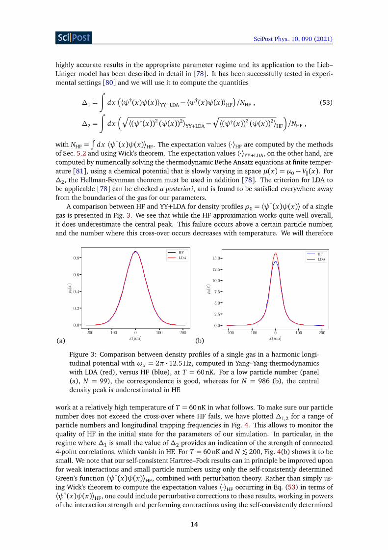
A comparison between HF and YY+LDA for density profiles ρ0 = ⟨ψ†(x)ψ(x)⟩ of a singlegas is presented in Fig. 3. We see that while the HF approximation works quite well overall,it does underestimate the central peak. This failure occurs above a certain particle number,and the number where this cross-over occurs decreases with temperature. We will therefore

(a)−200 −100 0 100 200

x(µm)

0.0

0.2

0.4

0.6

0.8

ρ0(x

)

HF

LDA

(b)−200 −100 0 100 200

x(µm)

0.0

2.5

5.0

7.5

10.0

12.5

15.0

ρ0(x

)

HF

LDA

Figure 3: Comparison between density profiles of a single gas in a harmonic longi-tudinal potential with ωx = 2π · 12.5 Hz, computed in Yang–Yang thermodynamicswith LDA (red), versus HF (blue), at T = 60 nK. For a low particle number (panel(a), N = 99), the correspondence is good, whereas for N = 986 (b), the centraldensity peak is underestimated in HF.

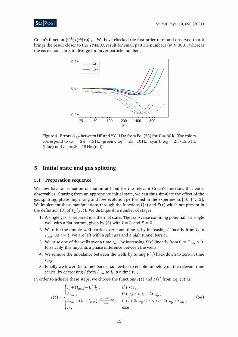
work at a relatively high temperature of T = 60nK in what follows. To make sure our particlenumber does not exceed the cross-over where HF fails, we have plotted ∆1,2 for a range ofparticle numbers and longitudinal trapping frequencies in Fig. 4. This allows to monitor thequality of HF in the initial state for the parameters of our simulation. In particular, in theregime where ∆1 is small the value of ∆2 provides an indication of the strength of connected4-point correlations, which vanish in HF. For T = 60 nK and N ® 200, Fig. 4(b) shows it to besmall. We note that our self-consistent Hartree–Fock results can in principle be improved uponfor weak interactions and small particle numbers using only the self-consistently determinedGreen’s function ⟨ψ†(x)ψ(x)⟩HF, combined with perturbation theory. Rather than simply us-ing Wick’s theorem to compute the expectation values ⟨·⟩HF occurring in Eq. (53) in terms of⟨ψ†(x)ψ(x)⟩HF, one could include perturbative corrections to these results, working in powersof the interaction strength and performing contractions using the self-consistently determined

14

SciPost Phys. 10, 090 (2021)

Green’s function ⟨ψ†(x)ψ(x)⟩HF. We have checked the first order term and observed that itbrings the result closer to the YY+LDA result for small particle numbers (N ® 300), whereasthe correction starts to diverge for larger particle numbers.

25 50 100 200 400 800N

-0.2

0.0

0.2 ∆1

∆2

Figure 4: Errors∆1,2 between HF and YY+LDA from Eq. (53) for T = 60 K. The colorscorrespond to ω‖ = 2π · 7.5Hz (green), ω‖ = 2π · 10Hz (cyan), ω‖ = 2π · 12.5Hz(blue) and ω‖ = 2π · 15 Hz (red).

5 Initial state and gas splitting

5.1 Preparation sequence

We now have an equation of motion at hand for the relevant Green’s functions that enterobservables. Starting from an appropriate initial state, we can thus simulate the effect of thegas splitting, phase imprinting and free evolution performed in the experiments [10, 14, 15].We implement these manipulations through the functions I(t) and F(t) which are present inthe definition (3) of V⊥(y, t). We distinguish a number of stages:

1. A single gas is prepared in a thermal state. The transverse confining potential is a singlewell with a flat bottom, given by (3) with I = Ic and F = 0.

2. We raise the double well barrier over some time tr by increasing I linearly from Ic toImax. At t = tr we are left with a split gas and a high tunnel barrier.

3. We raise one of the wells over a time timp by increasing F(t) linearly from 0 to Fmax > 0.Physically, this imprints a phase difference between the wells.

4. We remove the imbalance between the wells by tuning F(t) back down to zero in timetimp.

5. Finally we lower the tunnel barrier somewhat to enable tunneling on the relevant timescales, by decreasing I from Imax to If in a time tlow.

In order to achieve these steps, we choose the functions I(t) and F(t) from Eq. (3) as

I(t) =

Ic + (Imax − Ic)ttr

, if t < tr ,

Imax , if tr ≤ t < tr + 2timp ,

Imax + (If − Imax)t−tr−2timp

tlow, if tr + 2timp ≤ t < tr + 2timp + tlow ,

If , else ,

(54)

15

SciPost Phys. 10, 090 (2021)

and

F(t) =

0 , if t < tr ,t−trtimp

, if tr ≤ t < tr + timp ,

1− t−tr−timp

timp, if tr + timp ≤ t < tr + 2timp ,

0 , if tr + 2timp ≤ t ,

(55)

with tr = 5ms, timp = tlow = 2ms, Ic = 0.4, Imax = 0.58 and If = 0.5.

5.2 Numerical determination of the initial state

At stage 1, the system is initialized in a thermal state of the Hamiltonian (12), subject to theHF approximation (50). This state is determined as follows. We expand the field operators as

ψa(x) =∑

a,αχα(x)Φa(y)baα , (56)

where χα are real eigenfunctions of the harmonic oscillator potential in the x-direction, andwe keep nm + 1 such modes. The Hamiltonian (12) subject to (50) can then be written as

H(a)1D (0) =a−1∑

a,b=0

nm∑

α,β=0

haα,bβ b†aα bbβ , (57)

with the tensors

haα,bβ = δa,bδα,β [ωx (α+ 1/2) + εa(0)] + 4a−1∑

c,d=0

nm∑

γ,δ=0

Γabcd(0)Γαβγδ¬

b†cγ bdδ

¶

,

Γαβγδ =

∫

d x χα(x)χβ(x)χγ(x)χδ(x) . (58)

Reshaping haα,bβ and diagonalizing the resulting matrix numerically yields a canonical trans-formation

baα =∑

bβ Paα,bβ cbβ . (59)

The new creation and annihilation operators diagonalize the Hamiltonian H(a)1D (0) =∑

aα Eaαc†

aα caα. Assuming the c’s to have thermal occupation numbers with respect to this Hamiltonianthen gives

¬

b†cγ bdδ

¶

=∑

aα

P†cγ,aαPaα,dδ

e(Eaα−µ)/kBT − 1, (60)

which combined with (58) forms a self-consistent system of equations. We proceed by iter-ation: starting from an initial guess

b†cγ bdδ

�

0, which we take to be thermal with respect tothe non-interacting Hamiltonian, we diagonalize haα,bβ and compute (60) with the resultingP and E. Reinserting into (58) leads to the next iteration, and we repeat until convergence isreached.

A major hurdle in the above procedure is presented by the overlap tensor Γαβγδ. As weuse nm = 1000 modes, this tensor is too large to store numerically. However, using knownidentities for Hermite polynomials [77], we can write (58) as

Γαβγδ =p

mωx

2nm∑

p=0

Apαβ

Apγδ

, (61)

Apαβ=

min(α,β)∑

m=0

Bpmαβ

, (62)

16

SciPost Phys. 10, 090 (2021)

where the tensors Bpmαβ

are 0 if α+β −2m− p is odd and/or negative, and otherwise given by

Bpmαβ=

m!p

α!β!

2m

p2α+β

�

α

m

��

β

m

�

(α+ β − 2m)! (−1/2)12 (α+β−2m−p)

p

p! ((α+ β − 2m− p)/2)!. (63)

The considerably smaller tensors Apαβ

can now be separately contracted with other terms in(58), leading to a great memory gain. Even so, evaluating and storing the tensors (63) is stilla very slow process for nm = 1000. We therefore make a simplifying assumption: we set

Apαβ→ 0 if |α− β |> Λ (64)

for some Λ, which we choose to be 40 in our numerics. To see how this is justified, we notethat the Hamiltonian (57)-(58) implies the relation

[ωx (α+ 1/2) + εa(0)− Eaα]Paα,aα =

= 4∑

b,c,d

∑

β ,γ,δ

Γabcd(0)Γαβγδ∑

cγ

P†cγ,cγPcγ,dδ

e(Eaα−µ)/kBT − 1Pbβ ,aα

(65)

on the canonical transformations P for all a, a,α,α. The assumption (64) is therefore valid ifthe Paα,bβ become very small whenever |α−β |¦ Λ. This is reasonable since the weak interac-tions are not expected to couple harmonic oscillator modes that have widely different numbersof nodes. We check a posteriory that this assumption is consistent and well within the rangeset by Λ. We have also checked the assumption explicitly for the case of nm = 400. Finally,we have verified that the Green’s functions resulting from the above procedure remain time-independent when they are propagated in time under (51) with a time-independent potentialV⊥(y, 0).

The above procedure yields a set of Green’s functions Ci j(x , y) which characterize thestate of the system at t = 0. In the central region of the trap, with |x | < 3µm, we findexponential decay of the Green’s functions Cii(x ,−x) for the parameters presented in Sec. 6.1.The associated correlation length is roughly 0.5µm.

6 Josephson oscillations

We are now in a position to model the full experimental sequence. To do so, we first fix thevalues for various constants and parameters.

6.1 Experimental parameters

The transverse potential V⊥(y, t) is described by Eq. (3) and its time evolution follows Sec. 5.1with tr = 4 ms, timp = 2 ms and tlow = 2ms. This means that after a time tr+2timp+tlow = 11ms,the confining potential becomes time-independent, and the 1D field operators lose their ex-plicit time-dependence as a result. We consider a temperature of 60nK and take the transverseconfining potential in the z-direction to be harmonic with ωz = 2π ·1.7 kHz. The s-wave scat-tering length and atomic mass for the experimental system of 87Rb atoms [15] are as ≈ 5.2nmand m≈ 1.4 · 10−25kg, respectively. This fixes all parameters in the problem.

6.2 Assessment of time-dependent truncation errors in a toy model

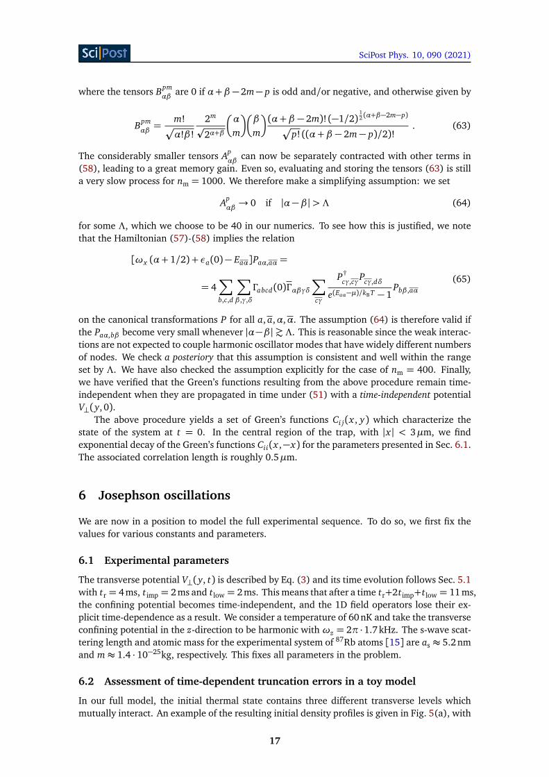
In our full model, the initial thermal state contains three different transverse levels whichmutually interact. An example of the resulting initial density profiles is given in Fig. 5(a), with

17

SciPost Phys. 10, 090 (2021)

(a)-100 -50 0 50 100

x(µm)

0

1

2

3Cii(x,x,0

)(µ

m−

1)

C00(x, x, 0)

C11(x, x, 0)

C22(x, x, 0)

(b)0 2 4 6 8 10 12

t (ms)

0.3

1.0

3.0

C(3)00

C(e)00

C(3)11

C(e)11

C(3)22

C(e)22

Figure 5: (a) Initial density profiles of levels 0,1, 2 at T = 60 nK, ωx = 2π · 12.5Hzand N = 259. (b) Time evolution of Green’s functions Cii = ⟨ψ

†i ψi⟩ for the quantum

mechanical problem of noninteracting bosons in a double well. This corresponds tothe PDE (51) in the absence of x-dependence and with Γi jkl = 0. We compare theproblem with truncation index a = 3 (as in the full model, solid curves) to resultsfor a = 15 (dotted curves). The latter is chosen by looking for convergence in a.The initial conditions match the peak densities from panel (a) at t = 0 and a verticallog-scale is chosen to highlight changes in C22.

occupation of the higher levels being suppressed as expected thanks to their larger energycost. For t > 0, the occupations can change in a way that is both due to interactions and tothe non-adiabaticity of the deformation of V⊥(y, t). The latter is modelled by the additionalterm (49) in the equations of motion (45), which are truncated at a = a = 3. To assess theerror made in this truncation, we briefly consider the quantum mechanical problem of bosonsin a double well V⊥(y, t). We discard the x-direction and set interactions to zero, so that theproblem is given by Eq. (51) in the absence of x-dependence and with Γi jkl = 0. This problemcan be integrated numerically for any value of the truncation index a. Results for a = 3 (as weuse in the full model) and a = 15 are compared in Fig. 5(b). The lines remain close, showingthat the truncation error has a very small effect on transitions induced by the time-dependenceof V⊥(y, t).

6.3 Characterization of the quantum state after the preparation sequence

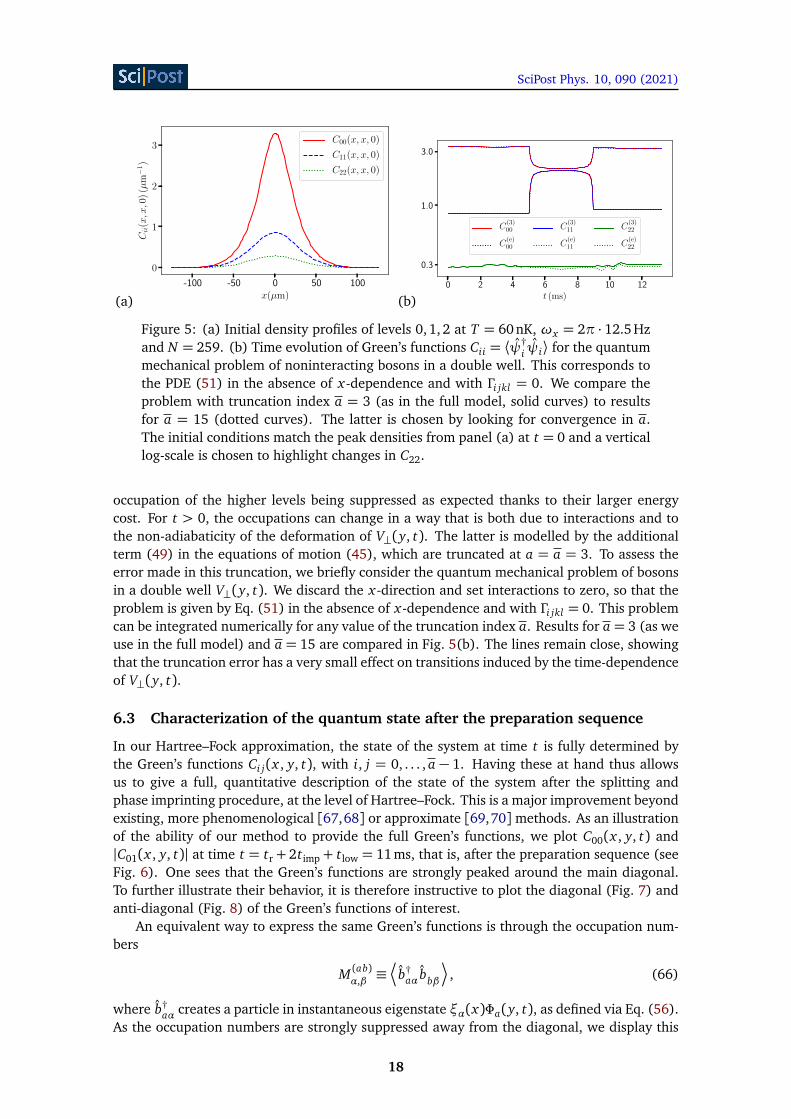
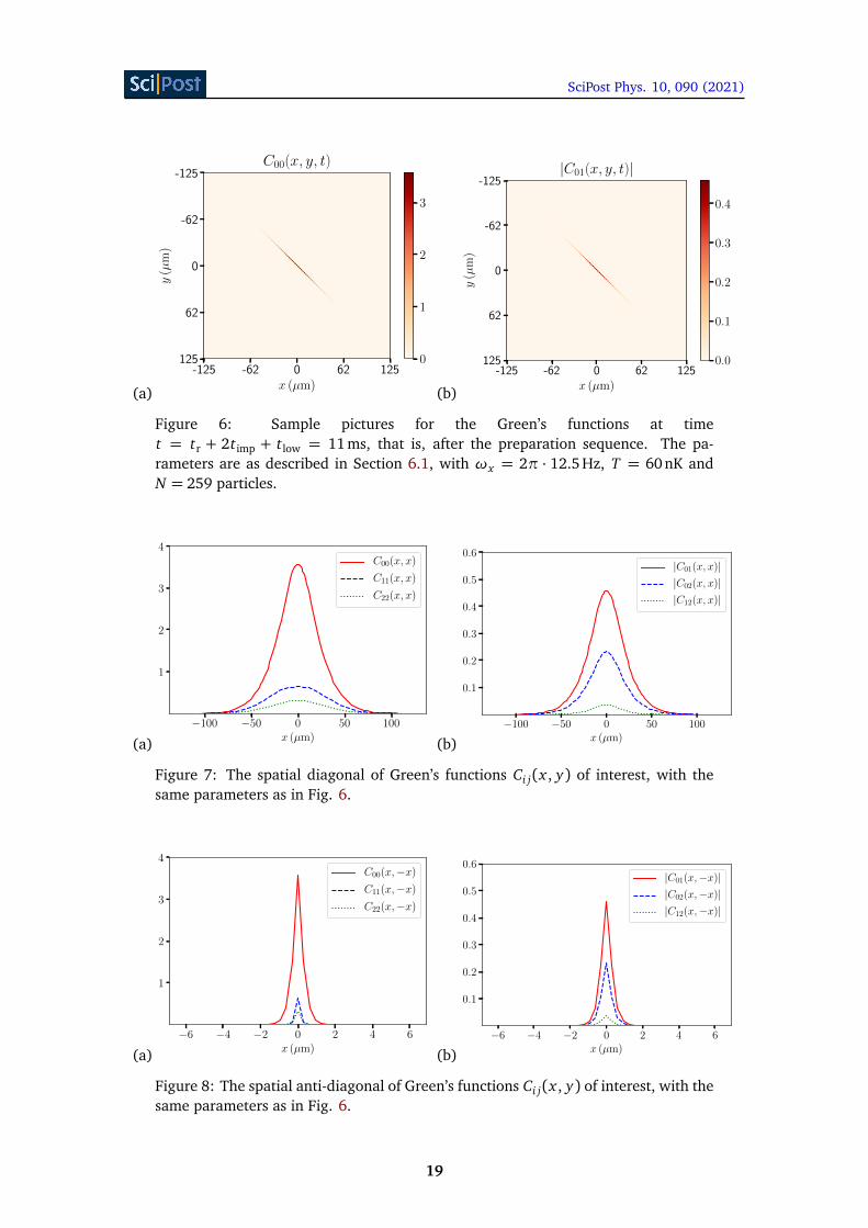
In our Hartree–Fock approximation, the state of the system at time t is fully determined bythe Green’s functions Ci j(x , y, t), with i, j = 0, . . . , a − 1. Having these at hand thus allowsus to give a full, quantitative description of the state of the system after the splitting andphase imprinting procedure, at the level of Hartree–Fock. This is a major improvement beyondexisting, more phenomenological [67,68] or approximate [69,70]methods. As an illustrationof the ability of our method to provide the full Green’s functions, we plot C00(x , y, t) and|C01(x , y, t)| at time t = tr + 2timp + tlow = 11ms, that is, after the preparation sequence (seeFig. 6). One sees that the Green’s functions are strongly peaked around the main diagonal.To further illustrate their behavior, it is therefore instructive to plot the diagonal (Fig. 7) andanti-diagonal (Fig. 8) of the Green’s functions of interest.

An equivalent way to express the same Green’s functions is through the occupation num-bers

M (ab)α,β ≡

¬

b†aα bbβ

¶

, (66)

where b†aα creates a particle in instantaneous eigenstate ξα(x)Φa(y, t), as defined via Eq. (56).

As the occupation numbers are strongly suppressed away from the diagonal, we display this

18

SciPost Phys. 10, 090 (2021)

(a)

-125 -62 0 62 125x (µm)

-125

-62

0

62

125

y(µ

m)

C00(x, y, t)

0

1

2

3

(b)

-125 -62 0 62 125x (µm)

-125

-62

0

62

125

y(µ

m)

|C01(x, y, t)|

0.0

0.1

0.2

0.3

0.4

Figure 6: Sample pictures for the Green’s functions at timet = tr + 2timp + tlow = 11 ms, that is, after the preparation sequence. The pa-rameters are as described in Section 6.1, with ωx = 2π · 12.5Hz, T = 60nK andN = 259 particles.

(a)−100 −50 0 50 100

x (µm)

1

2

3

4C00(x, x)

C11(x, x)

C22(x, x)

(b)−100 −50 0 50 100

x (µm)

0.1

0.2

0.3

0.4

0.5

0.6|C01(x, x)||C02(x, x)||C12(x, x)|

Figure 7: The spatial diagonal of Green’s functions Ci j(x , y) of interest, with thesame parameters as in Fig. 6.

(a)−6 −4 −2 0 2 4 6

x (µm)

1

2

3

4C00(x,−x)

C11(x,−x)

C22(x,−x)

(b)−6 −4 −2 0 2 4 6

x (µm)

0.1

0.2

0.3

0.4

0.5

0.6|C01(x,−x)||C02(x,−x)||C12(x,−x)|

Figure 8: The spatial anti-diagonal of Green’s functions Ci j(x , y) of interest, with thesame parameters as in Fig. 6.

19

SciPost Phys. 10, 090 (2021)

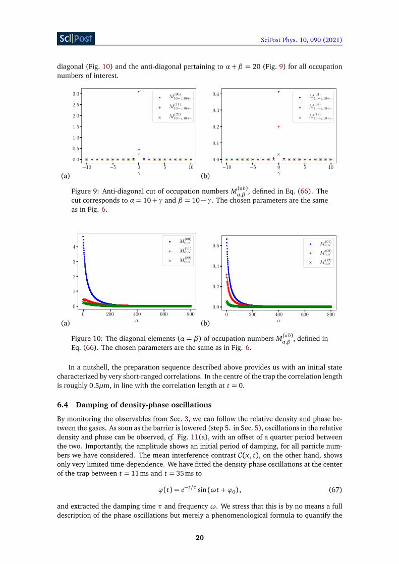
diagonal (Fig. 10) and the anti-diagonal pertaining to α+ β = 20 (Fig. 9) for all occupationnumbers of interest.

(a)−10 −5 0 5 10

γ

0.0

0.5

1.0

1.5

2.0

2.5

3.0M

(00)10−γ,10+γ

M(11)10−γ,10+γ

M(22)10−γ,10+γ

(b)−10 −5 0 5 10

γ

0.0

0.1

0.2

0.3

0.4 M(01)10−γ,10+γ

M(02)10−γ,10+γ

M(12)10−γ,10+γ

Figure 9: Anti-diagonal cut of occupation numbers M (ab)α,β , defined in Eq. (66). The

cut corresponds to α= 10+ γ and β = 10− γ. The chosen parameters are the sameas in Fig. 6.

(a)0 200 400 600 800

α

0

1

2

3

4M

(00)α,α

M(11)α,α

M(22)α,α

(b)0 200 400 600 800

α

0.0

0.2

0.4

0.6 M(01)α,α

M(02)α,α

M(12)α,α

Figure 10: The diagonal elements (α = β) of occupation numbers M (ab)α,β , defined in

Eq. (66). The chosen parameters are the same as in Fig. 6.

In a nutshell, the preparation sequence described above provides us with an initial statecharacterized by very short-ranged correlations. In the centre of the trap the correlation lengthis roughly 0.5µm, in line with the correlation length at t = 0.

6.4 Damping of density-phase oscillations

By monitoring the observables from Sec. 3, we can follow the relative density and phase be-tween the gases. As soon as the barrier is lowered (step 5. in Sec. 5), oscillations in the relativedensity and phase can be observed, cf. Fig. 11(a), with an offset of a quarter period betweenthe two. Importantly, the amplitude shows an initial period of damping, for all particle num-bers we have considered. The mean interference contrast C(x , t), on the other hand, showsonly very limited time-dependence. We have fitted the density-phase oscillations at the centerof the trap between t = 11ms and t = 35ms to

ϕ(t) = e−t/τ sin (ωt +ϕ0) , (67)

and extracted the damping time τ and frequency ω. We stress that this is by no means a fulldescription of the phase oscillations but merely a phenomenological formula to quantify the

20

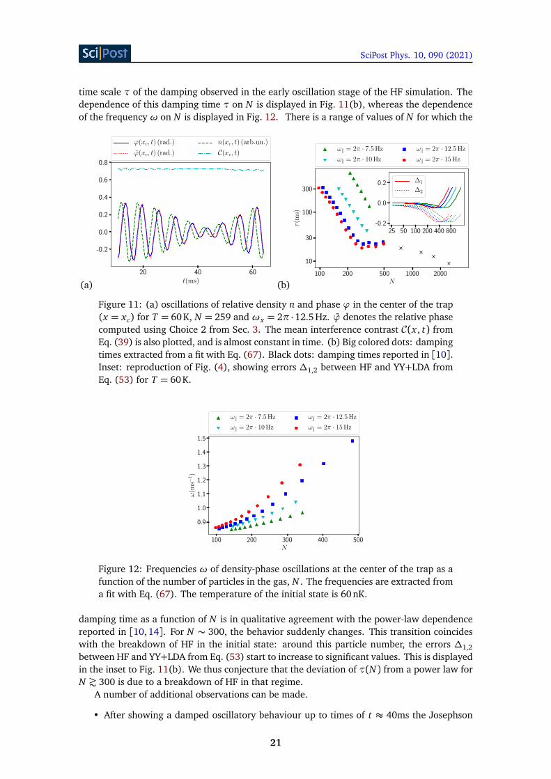
SciPost Phys. 10, 090 (2021)

time scale τ of the damping observed in the early oscillation stage of the HF simulation. Thedependence of this damping time τ on N is displayed in Fig. 11(b), whereas the dependenceof the frequency ω on N is displayed in Fig. 12. There is a range of values of N for which the

(a)20 40 60

t(ms)

-0.2

0.0

0.2

0.4

0.6

0.8

ϕ(xc, t) (rad.)

ϕ(xc, t) (rad.)

n(xc, t) (arb.un.)

C(xc, t)

(b)100 200 500 1000 2000

N

10

30

100

300

τ(m

s)

ω‖ = 2π · 7.5 Hz

ω‖ = 2π · 10 Hz

ω‖ = 2π · 12.5 Hz

ω‖ = 2π · 15 Hz

25 50 100 200 400 800-0.2

0.0

0.2 ∆1

∆2

Figure 11: (a) oscillations of relative density n and phase ϕ in the center of the trap(x = xc) for T = 60 K, N = 259 and ωx = 2π ·12.5 Hz. ϕ denotes the relative phasecomputed using Choice 2 from Sec. 3. The mean interference contrast C(x , t) fromEq. (39) is also plotted, and is almost constant in time. (b) Big colored dots: dampingtimes extracted from a fit with Eq. (67). Black dots: damping times reported in [10].Inset: reproduction of Fig. (4), showing errors ∆1,2 between HF and YY+LDA fromEq. (53) for T = 60K.

100 200 300 400 500N

0.9

1.0

1.1

1.2

1.3

1.4

1.5

ω(m

s−1)

ω‖ = 2π · 7.5 Hz

ω‖ = 2π · 10 Hz

ω‖ = 2π · 12.5 Hz

ω‖ = 2π · 15 Hz

Figure 12: Frequencies ω of density-phase oscillations at the center of the trap as afunction of the number of particles in the gas, N . The frequencies are extracted froma fit with Eq. (67). The temperature of the initial state is 60nK.

damping time as a function of N is in qualitative agreement with the power-law dependencereported in [10, 14]. For N ∼ 300, the behavior suddenly changes. This transition coincideswith the breakdown of HF in the initial state: around this particle number, the errors ∆1,2between HF and YY+LDA from Eq. (53) start to increase to significant values. This is displayedin the inset to Fig. 11(b). We thus conjecture that the deviation of τ(N) from a power law forN ¦ 300 is due to a breakdown of HF in that regime.

A number of additional observations can be made.

• After showing a damped oscillatory behaviour up to times of t ≈ 40ms the Josephson

21

SciPost Phys. 10, 090 (2021)

oscillations begin to increase again. This effect is not observed in the experiments, whichas we have stressed throughout have been performed in a different parameter regimenot accessible by HF. We note however, that the experiments focused on time scales ofbelow 40−60ms, so that it cannot be ruled out that at later times a reemergence of theoscillations occurs in the experimentally relevant parameter regime as well. It would beinteresting to repeat the experiments for lower particle numbers in order to study thisreemergence in detail.

• The frequency of density-phase oscillations is highest at the center xc of the trap in thex-direction. Away from this point, the frequency is smaller, as displayed in Fig. 13(a).This figure also shows that the damping during the first few periods is somewhat weaker

(a)20 40 60 80 100 120

t(ms)

−0.3

−0.2

−0.1

0.0

0.1

0.2

0.3

ϕ(xc) ϕ(x1) ϕ(x2) (rad.)

(b)20 40 60 80 100 120

t(ms)

550

600

650

700

⟨(x− xc)2

⟩t,L

(µm2)

⟨(x− xc)2

⟩t,R

(µm2)

Figure 13: Additional plots for the same parameters as Fig. 11(a). (a) relative phaseat the trap center (x = xc) and at positions x1 = xc +25µm, x2 = xc +37.5µm. (b)squared longitudinal size (68) of left and right gases (red and green) as well as theiraverage (black).

at points away from the trap center, where the gas density is smaller.

• The gas as a whole shows a breathing motion. This can be shown by studying the squaredlongitudinal size of the left and right gas profiles,

(x − xc)2�

t,i ≡∫

d x Cii(x , x , t) (x − xc)2 /

∫

d x Cii(x , x , t), i = L, R . (68)

Fig. 13(b) shows that the squared longitudinal sizes of the left and right gases oscillateout of phase with one another. On top of this, there is an overall breathing motion of thegas with a frequency that depends monotonously on ωx . This breathing gets dampedover a timescale that is large compared to the breathing period of the separate left andright gases.

• The time scale of the breathing motion of the gas is seen to coincide with the time atwhich the Josephson oscillations reemerge after the initial oscillatory decay.

It is instructive to investigate the effect on the damping that various aspects of our set-upmight have. First, there are two possible definitions of left- and right-localized bosons ψL,R,as described in Sec. 3. As mentioned there, we stick to Choice 1 (cf. (36)) by default. Do ourresults, and the observed damping in particular, change if we switch to Choice 2? Fig. 11(a)shows results for Choice 2 in red. The curve is shown to lie very close to the blue curve, whichwas computed with Choice 1. This behavior occurred for all performed simulations, showingthat the choice between Choices 1 and 2 does not significantly affect our results.

22

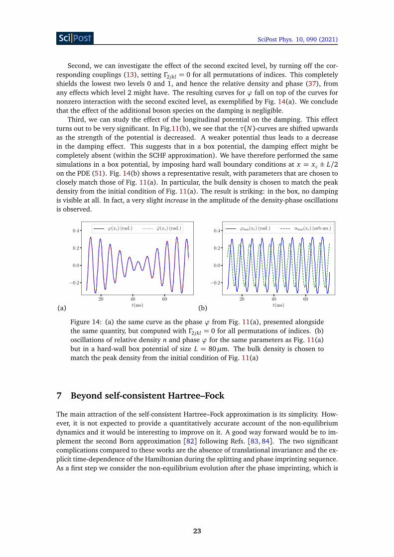
SciPost Phys. 10, 090 (2021)

Second, we can investigate the effect of the second excited level, by turning off the cor-responding couplings (13), setting Γ2 jkl = 0 for all permutations of indices. This completelyshields the lowest two levels 0 and 1, and hence the relative density and phase (37), fromany effects which level 2 might have. The resulting curves for ϕ fall on top of the curves fornonzero interaction with the second excited level, as exemplified by Fig. 14(a). We concludethat the effect of the additional boson species on the damping is negligible.

Third, we can study the effect of the longitudinal potential on the damping. This effectturns out to be very significant. In Fig.11(b), we see that the τ(N)-curves are shifted upwardsas the strength of the potential is decreased. A weaker potential thus leads to a decreasein the damping effect. This suggests that in a box potential, the damping effect might becompletely absent (within the SCHF approximation). We have therefore performed the samesimulations in a box potential, by imposing hard wall boundary conditions at x = xc ± L/2on the PDE (51). Fig. 14(b) shows a representative result, with parameters that are chosen toclosely match those of Fig. 11(a). In particular, the bulk density is chosen to match the peakdensity from the initial condition of Fig. 11(a). The result is striking: in the box, no dampingis visible at all. In fact, a very slight increase in the amplitude of the density-phase oscillationsis observed.

(a)20 40 60

t(ms)

−0.2

0.0

0.2

0.4ϕ(xc) (rad.) ϕ(xc) (rad.)

(b)20 40 60

t(ms)

−0.2

0.0

0.2

0.4ϕbox(xc) (rad.) nbox(xc) (arb.un.)

Figure 14: (a) the same curve as the phase ϕ from Fig. 11(a), presented alongsidethe same quantity, but computed with Γ2 jkl = 0 for all permutations of indices. (b)oscillations of relative density n and phase ϕ for the same parameters as Fig. 11(a)but in a hard-wall box potential of size L = 80µm. The bulk density is chosen tomatch the peak density from the initial condition of Fig. 11(a)

7 Beyond self-consistent Hartree–Fock

The main attraction of the self-consistent Hartree–Fock approximation is its simplicity. How-ever, it is not expected to provide a quantitatively accurate account of the non-equilibriumdynamics and it would be interesting to improve on it. A good way forward would be to im-plement the second Born approximation [82] following Refs. [83, 84]. The two significantcomplications compared to these works are the absence of translational invariance and the ex-plicit time-dependence of the Hamiltonian during the splitting and phase imprinting sequence.As a first step we consider the non-equilibrium evolution after the phase imprinting, which is

23

SciPost Phys. 10, 090 (2021)

described by a time-independent Hamiltonian (12)

H1D =a−1∑

a=0

∫

d x ψ†a(x)

�

−1

2m∂ 2

∂ x2+

mω2

2x2 + εa

�

ψa(x)

+

∫

d xa−1∑

a,b,c,d=0

Γabcd ψ†a(x)ψ

†b(x)ψc(x)ψd(x) . (69)

We now expand in harmonic oscillator modes notation

ψa(x) =∑

j

χ j(x)ba, j , (70)

and substitute this back into the expression for the Hamiltonian. Introducing a multi-index

k ≡ (a, j) , ba, j = b(k) , (71)

we can rewrite the Hamiltonian in a very compact form

H1D =∑

k

ε(k)b†(k)b(k) +∑

k1,k1,k3,k4

V (k1, k2, k3, k4) b†(k1)b†(k2)b(k3)b(k4). (72)

Here we have defined

ε(k) = εa + ε j , V (k1, k2, k3, k4) = Γabcd Γi jkl , (73)

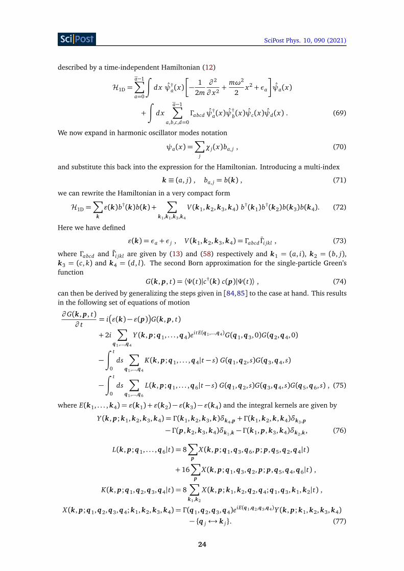
where Γabcd and Γi jkl are given by (13) and (58) respectively and k1 = (a, i), k2 = (b, j),k3 = (c, k) and k4 = (d, l). The second Born approximation for the single-particle Green’sfunction

G(k, p, t) = ⟨Ψ(t)|c†(k) c(p)|Ψ(t)⟩ , (74)

can then be derived by generalizing the steps given in [84,85] to the case at hand. This resultsin the following set of equations of motion

∂ G(k, p, t)∂ t

= i�

ε(k)− ε(p)�

G(k, p, t)

+ 2i∑

q1,...,q4

Y (k, p;q1, . . . ,q4)ei tE(q1,...,q4)G(q1,q3, 0)G(q2,q4, 0)

−∫ t

0

ds∑

q1,...,q4

K(k, p;q1, . . . ,q4|t − s) G(q1,q2, s)G(q3,q4, s)

−∫ t

0

ds∑

q1,...,q6

L(k, p;q1, . . . ,q6|t − s) G(q1,q2, s)G(q3,q4, s)G(q5,q6, s) , (75)

where E(k1, . . . , k4) = ε(k1) + ε(k2)− ε(k3)− ε(k4) and the integral kernels are given by

Y (k, p; k1, k2, k3, k4) = Γ (k1, k2, k3, k)δk4,p + Γ (k1, k2, k, k4)δk3,p

− Γ (p, k2, k3, k4)δk1,k − Γ (k1, p, k3, k4)δk2,k , (76)

L(k, p;q1, . . . ,q6|t) = 8∑

p

X (k, p;q1,q3,q6, p; p,q5,q2,q4|t)

+ 16∑

p

X (k, p;q1,q3,q2, p; p,q5,q4,q6|t) ,

K(k, p;q1,q2,q3,q4|t) = 8∑

k1,k2

X (k, p; k1, k2,q2,q4;q1,q3, k1, k2|t) ,

X (k, p;q1,q2,q3,q4; k1, k2, k3, k4) = Γ (q1,q2,q3,q4)eiE(q1,q2,q3,q4)Y (k, p; k1, k2, k3, k4)

− {q j ↔ k j}. (77)

24

SciPost Phys. 10, 090 (2021)

The set of integro-differential equations (75) is clearly much more difficult to solve numericallythan the self-consistent Hartree–Fock equations. The time integration is crucial at short times,while for sufficiently late times (75) ought to be reducible to a matrix quantum Boltzmannequation [84]. Integrating (75) is beyond the scope of this paper, but some general commentsare in order. It is clear that in order to be able to integrate (75) numerically only a limitednumber of different k modes can be retained. Hence one should focus on the case wherethe longitudinal confinement is fairly tight. In this (experimentally readily accessible) caseinteraction effects beyond the SCHF approximation can be analyzed through (75).

8 Conclusions

In this work we have developed a microscopic theory for the non-equilibrium evolution ofbosons confined by a time-dependent quasi-one-dimensional trapping potential. Using that thetransverse confinement is tight we have projected the full three-dimensional theory to a finitenumber of coupled, one-dimensional channels. By employing a time-dependent projection thenumber of channels that need to be retained in experimentally relevant parameter regimes isvery small: three channels suffice. We then analyzed the resulting theory by means of a self-consistent time-dependent Hartree–Fock approximation and showed how the resulting Green’sfunctions are related to averages of experimentally measured quantities. The Hartree–Fockapproximation is expected to apply only for sufficiently weak interactions and sufficiently highenergy densities. We have tried to identify a corresponding parameter regime by comparing theSCHF approximation to results obtained by combining the exact solution of the Lieb-Linigermodel with a local density approximation in the trapping potential. On the basis of theseconsiderations we restricted our initial states to temperatures of at least 60 nK and to particlenumbers below ∼ 200. In this parameter regime we expect the HF method to work well atleast at short times, when the neglected higher connected n-point functions have not had timeto grow substantially.

Our method has a number of attractive features. First, it allows to include the effects ofvarious longitudinal potentials. Second, it can account for higher excited levels of the trans-verse confining potential which are normally neglected. Finally, it allows us to model the gassplitting and phase imprinting in a fully microscopic way. To our knowledge, such a model hasnot been presented before, and one of our main results is a characterization of the quantumstate of the system after gas splitting and phase imprinting in terms of single-particle Green’sfunctions of the one-dimensional channels. The second main result of our work is the descrip-tion of the density-phase oscillations that ensue after the splitting and phase imprinting. Inparticular we find that these are damped over a few oscillation periods. These damped oscilla-tions agree with recent measurements [10,14,15] in multiple ways. First, the damping time isinversely related to the number of particles, following a curve compatible with [10]. Second,the oscillation frequency decreases away from the center of the trap, as observed in [15]. Wehave shown that the coupling to the second excited level has very little effect on the damp-ing. On the other hand, the longitudinal trapping potential is seen to play a very importantrole: the weaker the longitudinal trapping frequency, the weaker the damping. In a hard wallbox, no damping is observed at all within our Hartree–Fock approximation. This suggests thatdamping effects are suppressed in this geometry for weak interactions. It therefore would bevery interesting to repeat the experiments [10, 14, 15] in a hard-wall box potential. Such po-tentials are indeed under development [12,16] and our model can serve as a direct theoreticalprediction for such setups.

The main limitation of our method is the way interactions are treated. In order to ac-cess the parameter regime of the experiments [10, 14, 15], in which the particle number was

25

SciPost Phys. 10, 090 (2021)

significantly higher than in our simulations, it is necessary to go beyond the SCHF approxi-mation used here. A major improvement can be provided by the second Born approximationdiscussed in section 7, but this is much harder to implement numerically. Ideally one wouldwant to employ a controlled approximation scheme like [86,87] for our fully time-dependentproblem.

Our work has several implications for attempts to describe Josephson oscillations in tunnel-coupled one-dimensional Bose gases based on the sine-Gordon model. Firstly, our work sug-gests that the experimental protocol for splitting and phase imprinting does not lead to a strongpopulation of higher transverse levels as long as the effective temperature of the initial ther-mal state is sufficiently low. This implies that a description in terms of a low-energy effectivefield theory based on a sine-Gordon model with appropriate perturbations should apply. Thereare several kinds of perturbations that should be considered. A key finding of our work is thestrong effect the longitudinal confining potential has on the damping of Josephson oscillationsin the parameter regime studied here. This suggests that the low-energy field theory calcu-lations based on the sine-Gordon model [62, 64–66] should be extended to account for thelongitudinal confinement. This is certainly possible in the framework of the self-consistenttime-dependent harmonic approximation used in [62,66]. Apart from the confining potentialthere are other perturbations to the sine-Gordon model that should be analysed. In particularone should consider the effects of the nonlinearities that arise from the curvature terms in thekinetic energy of the split Bose gas. These are formally irrelevant in equilibrium but could wellplay an important role in non-equilibrium dynamics.

Secondly, our characterization of the “initial state” after splitting and phase imprinting pro-vides very useful information on what initial states to consider in the sine-Gordon framework.In the first instance one should consider Gaussian states with very short correlation lengthsthat reproduce the single-particle Green’s functions reported here. Our microscopic modellingof the splitting process enables us to provide the same kind of information also in previouslystudied cases without phase-imprinting.

Acknowledgements

We are grateful to the Erwin Schrödinger International Institute for Mathematics and Physicsfor hospitality and support during the programme on Quantum Paths. This work was supportedby the EPSRC under grant EP/S020527/1 and YDvN is supported by the Merton College Buc-kee Scholarship and the VSB, Muller and Prins Bernhard Foundations. JS acknowledges thesupport by the Austrian Science Fund (FWF) via the DFG-FWF SFB 1225 ISOQUANT (I 3010-N27).

A Low energy projection in equilibrium

For simplicity we consider a two-dimensional system with time-independent Hamiltonian

H =

∫

d x d y

�

Ψ†(x , y)

�

−∇2

2m+

mω2

2x2 + V⊥(y)

�

Ψ(x , y) + c�

Ψ†(x , y)�2�Ψ(x , y)

�2�

. (78)

The quadratic part can be diagonalized by going to a basis of single-particle eigenstates

Ψ(x , y) =∞∑

j,k=0

χ j(x)Φk(y) b j,k . (79)

26

SciPost Phys. 10, 090 (2021)

Here χ j(x) are harmonic oscillator wave functions and Φk(y) are orthonormal eigenstates ofthe Hamiltonian H y

H y = −1

2md2

d y2+ V⊥(y) , H yΦk(y) = εkΦk(y) . (80)

In terms of the new canonical Bose fields

Ψk(x) =

∫

d y Φ∗k(y)Ψ(x , y) , [Ψ j(x),Ψk(x′)] = δ j,kδ(x − x ′) (81)

the Hamiltonian becomes

H =

∫

d x∞∑

k=0

Ψ†k(x) hk Ψk(x) +

∫

d x∞∑

k1,k2,k3,k4=0

Vk1,k2,k3,k4Ψ†

k1(x)Ψ†

k2(x)Ψk3

(x)Ψk4(x) . (82)

Here we have defined

hk =

�

−1

2m∂ 2

∂ x2+

mω2

2x2 + εk

�

,

Vk1,k2,k3,k4= c

∫

d yΦ∗k1(y)Φ∗k2

(y)Φk3(y)Φk4

(y) . (83)

The imaginary time path integral representation of the partition function is

Z(β) =

∫ ∞∏

k=0

Dψ∗k(τ, x) Dψk(τ, x) e−S[ψ∗n,ψn] , (84)

where

S[ψ∗n,ψn] =

∫ β

0

dτ

∫

d x§ ∞∑

k=0

ψ∗k(τ, x)�

∂

∂ τ+ hk

�

ψk(τ, x) (85)

+∞∑

k1,k2,k3,k4=0

Vk1,k2,k3,k4ψ†

k1(τ, x)ψ†

k2(τ, x)ψk3

(τ, x)ψk4(τ, x)

ª

.

The situation we are interested in is where the eigenvalues εk of the transverse confiningpotential constitute a large energy scale and the transverse level spacings |εk − ε j| betweenhighly excited transverse states are large too. We can then “integrate out” the transversedegrees of freedom above some cutoff Λ. Let us denote the first eigenvalue above Λ by εa,and rewrite the action as

S[ψ∗n,ψn] = S< + S> + Sint , (86)

where S< is the part of the action that only involve the fields Ψk, Ψ†k with 0 ≤ k < a, S> the

quadratic part of the action that involves only fields with k ≥ a, and Sint are the remainingquartic terms that mix channels below and above the cutoff and describe interactions betweenchannels above the cutoff. Defining

⟨O⟩> =∫ ∞∏

k=a

Dψ∗k(τ, x) Dψk(τ, x) O e−S> , (87)

we can eliminate the degrees of freedom above the cutoff using that we are dealing with weakinteractions. Up to second order in Sint we have the following expression for the low-energypart of the action

Seff = S< + ⟨Sint⟩> −12

�

⟨S2int⟩> − ⟨Sint⟩2>

�

. (88)

27

SciPost Phys. 10, 090 (2021)

The first order term generates hopping between the low-energy channels

⟨Sint⟩> =∫ β

0

dτ

∫

d xa−1∑

k1,k2=0

Wk1,k2ψ†

k1(τ, x)ψk2

(τ, x) , (89)

where

Wk1,k2=∞∑

n=a

4Vn,k1,n,k2

∞∑

j=0

|χ j(x)|2

eβ�

εk+ω( j+1/2)�

− 1. (90)

We see that this is small compared to the interaction strength c because the Bose occupationfactors are by construction negligible. The second order term in Sint contains all possiblequadratic, quartic and sextic interactions involving ψk(x ,τ) and ψ∗k(x ,τ) compatible withparticle number conservation, e.g.

a−1∑

k1,k2,k3,k4=0

∫

dτ

∫

dτ′∫

d x

∫

d x ′ Uk1,k2,k3,k4(τ−τ′, x , x ′)

× ψ∗k1(τ, x)ψk2

(τ, x)ψ∗k3(τ′, x ′)ψk4

(τ′, x ′) , (91)

where

Uk1,k2,k3,k4(τ−τ′, x , x ′) = −8

∞∑

n2,n2=a

Vn1,k1,n2,k2Vn2,k3,n1,k4

× Gn1(τ′ −τ, x ′, x)Gn2

(τ−τ′, x , x ′) ,

Gk(τ > 0, x , x ′) =∑

j

χ j(x)χ∗j (x′)

e−τ�

εk+ω( j+1/2)�

1− e−β�

εk+ω( j+1/2)� = Gk(τ− β , x , x ′). (92)

As εk > Λ the Matsubara Green’s function of the high energy channels is very short-rangedin both imaginary time and space, so that retardation effects can be neglected and workingwith a purely local interaction between the low-energy channels remains justified. Hencethe quartic terms generate only a very small renormalization of the interaction terms alreadypresent between the low-energy channels.

References

[1] T. Kinoshita, T. Wenger and D. S. Weiss, A quantum Newton’s cradle, Nature 440, 900(2006), doi:10.1038/nature04693.

[2] S. Hofferberth, I. Lesanovsky, B. Fischer, T. Schumm and J. Schmiedmayer, Non-equilibrium coherence dynamics in one-dimensional Bose gases, Nature 449, 324 (2007),doi:10.1038/nature06149.

[3] E. Haller, M. Gustavsson, M. J. Mark, J. G. Danzl, R. Hart, G. Pupillo and H.-C. Nagerl, Re-alization of an excited, strongly correlated quantum gas phase, Science 325, 1224 (2009),doi:10.1126/science.1175850.

[4] S. Trotzky, Y.-A. Chen, A. Flesch, I. P. McCulloch, U. Schollwöck, J. Eisert and I.Bloch, Probing the relaxation towards equilibrium in an isolated strongly correlated one-dimensional Bose gas, Nat. Phys. 8, 325 (2012), doi:10.1038/nphys2232.

28

SciPost Phys. 10, 090 (2021)

[5] M. Gring et al., Relaxation and prethermalization in an isolated quantum system, Science337, 1318 (2012), doi:10.1126/science.1224953.

[6] T. Langen, R. Geiger, M. Kuhnert, B. Rauer and J. Schmiedmayer, Local emergence ofthermal correlations in an isolated quantum many-body system, Nat. Phys. 9, 640 (2013),doi:10.1038/nphys2739.

[7] J. P. Ronzheimer, M. Schreiber, S. Braun, S. S. Hodgman, S. Langer, I. P. McCulloch, F.Heidrich-Meisner, I. Bloch and U. Schneider, Expansion dynamics of interacting bosons inhomogeneous lattices in one and two dimensions, Phys. Rev. Lett. 110, 205301 (2013),doi:10.1103/PhysRevLett.110.205301.

[8] F. Meinert, M. J. Mark, E. Kirilov, K. Lauber, P. Weinmann, M. Gröbner and H.-C. Nägerl,Interaction-induced quantum phase revivals and evidence for the transition to the quan-tum chaotic regime in 1D atomic Bloch oscillations, Phys. Rev. Lett. 112, 193003 (2014),doi:10.1103/PhysRevLett.112.193003.

[9] Y. Tang, A. G. Sykes, N. Q. Burdick, J. M. DiSciacca, D. S. Petrov and B. L. Lev,Anisotropic expansion of a thermal dipolar Bose gas, Phys. Rev. Lett. 117, 155301 (2016),doi:10.1103/PhysRevLett.117.155301.

[10] M. Pigneur, T. Berrada, M. Bonneau, T. Schumm, E. Demler and J. Schmiedmayer, Relax-ation to a phase-locked equilibrium state in a one-dimensional bosonic Josephson junction,Phys. Rev. Lett. 120, 173601 (2018), doi:10.1103/PhysRevLett.120.173601.

[11] T. Schweigler et al., Experimental characterization of a quantum many-body system viahigher-order correlations, Nature 545, 323 (2017), doi:10.1038/nature22310.

[12] B. Rauer, S. Erne, T. Schweigler, F. Cataldini, M. Tajik and J. Schmiedmayer, Re-currences in an isolated quantum many-body system, Science 360, 307 (2018),doi:10.1126/science.aan7938.

[13] Y. Tang, W. Kao, K.-Y. Li, S. Seo, K. Mallayya, M. Rigol, S. Gopalakrishnan and B. L. Lev,Thermalization near integrability in a dipolar quantum Newton’s cradle, Phys. Rev. X 8,021030 (2018), doi:10.1103/PhysRevX.8.021030.

[14] M. Pigneur, Relaxation to a phase-locked equilibrium state in a ne-dimensional bosonicJosephson junction, PhD thesis, (2019).

[15] T. Schweigler, Correlations and dynamics of tunnel-coupled ne-dimensional Bose gases, PhDthesis, (2019).

[16] M. Tajik, B. Rauer, T. Schweigler, F. Cataldini, J. Sabino, F. S. Møller, S.-C. Ji, I. E. Mazetsand J. Schmiedmayer, Designing arbitrary one-dimensional potentials on an atom chip,Opt. Express 27, 33474 (2019), doi:10.1364/OE.27.033474.

[17] A. Polkovnikov, K. Sengupta, A. Silva and M. Vengalattore, Colloquium: Nonequilib-rium dynamics of closed interacting quantum systems, Rev. Mod. Phys. 83, 863 (2011),doi:10.1103/RevModPhys.83.863.

[18] F. H. L. Essler and M. Fagotti, Quench dynamics and relaxation in isolated in-tegrable quantum spin chains, J. Stat. Mech. 064002 (2016), doi:10.1088/1742-5468/2016/06/064002.

[19] L. Vidmar and M. Rigol, Generalized Gibbs ensemble in integrable lattice models, J. Stat.Mech. 064007 (2016), doi:10.1088/1742-5468/2016/06/064007.

29

SciPost Phys. 10, 090 (2021)

[20] L. D’Alessio, Y. Kafri, A. Polkovnikov and M. Rigol, From quantum chaos and eigenstatethermalization to statistical mechanics and thermodynamics, Adv. Phys. 65, 239 (2016),doi:10.1080/00018732.2016.1198134.

[21] C. Gogolin and J. Eisert, Equilibration, thermalisation, and the emergence of sta-tistical mechanics in closed quantum systems, Rep. Prog. Phys. 79, 056001 (2016),doi:10.1088/0034-4885/79/5/056001.

[22] P. Calabrese and J. Cardy, Quantum quenches in 1+1 dimensional conformal field theories,J. Stat. Mech. 064003 (2016), doi:10.1088/1742-5468/2016/06/064003.

[23] M. Olshanii, Atomic scattering in the presence of an external confinement and a gas ofimpenetrable bosons, Phys. Rev. Lett. 81, 938 (1998), doi:10.1103/PhysRevLett.81.938.

[24] E. H. Lieb and W. Liniger, Exact analysis of an interacting Bose gas. I. The general solutionand the ground state, Phys. Rev. 130, 1605 (1963), doi:10.1103/PhysRev.130.1605.

[25] M. A. Cazalilla, Bosonizing one-dimensional cold atomic gases, J. Phys. B: At. Mol. Opt.Phys. 37, S1 (2004), doi:10.1088/0953-4075/37/7/051.

[26] F. H. Essler and R. M. Konik, Application of massive integrable quantum field theo-ries to problems in condensed matter physics, in From Fields to Strings: Circumnavi-gating Theoretical Physics, World Scientific, Singapore, ISBN 9789812389558 (2005),doi:10.1142/9789812775344_0020.

[27] C. Karrasch, J. Rentrop, D. Schuricht and V. Meden, Luttinger-liquid universality inthe time evolution after an interaction quench, Phys. Rev. Lett. 109, 126406 (2012),doi:10.1103/PhysRevLett.109.126406.

[28] E. Coira, F. Becca and A. Parola, Quantum quenches in one-dimensional gapless systems,Eur. Phys. J. B 86, 55 (2013), doi:10.1140/epjb/e2012-30978-y.

[29] A. Mitra, Correlation functions in the prethermalized regime after a quantum quench of aspin chain, Phys. Rev. B 87, 205109 (2013), doi:10.1103/PhysRevB.87.205109.

[30] M. Collura, P. Calabrese and F. H. L. Essler, Quantum quench within the gaplessphase of the spin-1/2 Heisenberg XXZ spin chain, Phys. Rev. B 92, 125131 (2015),doi:10.1103/PhysRevB.92.125131.

[31] A. Imambekov, V. Gritsev and E. Demler, Fundamental noise in matter interferometers(2007), arXiv:cond-mat/0703766.

[32] T. Kitagawa, S. Pielawa, A. Imambekov, J. Schmiedmayer, V. Gritsev and E. Demler,Ramsey interference in one-dimensional systems: The full distribution function of fringecontrast as a probe of many-body dynamics, Phys. Rev. Lett. 104, 255302 (2010),doi:10.1103/PhysRevLett.104.255302.

[33] T. Kitagawa, A. Imambekov, J. Schmiedmayer and E. Demler, The dynamics andprethermalization of one-dimensional quantum systems probed through the full dis-tributions of quantum noise, New J. Phys. 13, 073018 (2011), doi:10.1088/1367-2630/13/7/073018.

[34] I. Lovas, B. Dóra, E. Demler and G. Zaránd, Full counting statistics of time-of-flight images,Phys. Rev. A 95, 053621 (2017), doi:10.1103/PhysRevA.95.053621.

30

SciPost Phys. 10, 090 (2021)

[35] M. Collura, F. H. L. Essler and S. Groha, Full counting statistics in the spin-1/2 Heisen-berg XXZ chain, J. Phys. A: Math. Theor. 50, 414002 (2017), doi:10.1088/1751-8121/aa87dd.

[36] K. Najafi and M. A. Rajabpour, Full counting statistics of the subsystem energyfor free fermions and quantum spin chains, Phys. Rev. B 96, 235109 (2017),doi:10.1103/PhysRevB.96.235109.

[37] A. Bastianello, L. Piroli and P. Calabrese, Exact local correlations nd full counting statis-tics for arbitrary states of the one-dimensional interacting Bose gas, Phys. Rev. Lett. 120,190601 (2018), doi:10.1103/PhysRevLett.120.190601.

[38] Y. D. van Nieuwkerk, J. Schmiedmayer and F. H. L. Essler, Projective phasemeasurements in one-dimensional Bose gases, SciPost Phys. 5, 046 (2018),doi:10.21468/SciPostPhys.5.5.046.

[39] M. Arzamasovs and D. M. Gangardt, Full counting statistics and large de-viations in a thermal 1D Bose gas, Phys. Rev. Lett. 122, 120401 (2019),doi:10.1103/PhysRevLett.122.120401.

[40] M. Collura and F. H. L. Essler, How order melts after quantum quenches, Phys. Rev. B 101,041110 (2020), doi:10.1103/PhysRevB.101.041110.

[41] M. Albiez, R. Gati, J. Fölling, S. Hunsmann, M. Cristiani and M. K. Oberthaler, Directobservation of tunneling and nonlinear self-trapping in a single bosonic Josephson junction,Phys. Rev. Lett. 95, 010402 (2005), doi:10.1103/PhysRevLett.95.010402.

[42] R. Gati, M. Albiez, J. Fölling, B. Hemmerling and M. K. Oberthaler, Realization of asingle Josephson junction for Bose-Einstein condensates, Appl. Phys. B 82, 207 (2006),doi:10.1007/s00340-005-2059-z.

[43] S. Levy, E. Lahoud, I. Shomroni and J. Steinhauer, The a.c. and d.c. Josephson effects in aBose-Einstein condensate, Nature 449, 579 (2007), doi:10.1038/nature06186.

[44] S. Hofferberth, I. Lesanovsky, B. Fischer, T. Schumm and J. Schmiedmayer, Non-equilibrium coherence dynamics in one-dimensional Bose gases, Nature 449, 324 (2007),doi:10.1038/nature06149.

[45] V. Gritsev, A. Polkovnikov and E. Demler, Linear response theory for a pair of cou-pled one-dimensional condensates of interacting atoms, Phys. Rev. B 75, 174511 (2007),doi:10.1103/PhysRevB.75.174511.

[46] A. B. Zamolodchikov, Exact two-particle S-matrix of quantum sine-Gordon solitons, Com-mun. Math. Phys. 55, 183 (1977), doi:10.1007/BF01626520.

[47] H. Bergknoff and H. B. Thacker, Structure and solution of the massive Thirring model,Phys. Rev. D 19, 3666 (1979), doi:10.1103/PhysRevD.19.3666.

[48] V. E. Korepin, Direct calculation of the S matrix in the massive Thirring model, Theor. Math.Phys. 41, 953 (1979), doi:10.1007/BF01028501.

[49] M. Oshikawa and I. Affleck, Field-induced gap S = 1/2 antiferromagnetic chains, Phys.Rev. Lett. 79, 2883 (1997), doi:10.1103/PhysRevLett.79.2883.

[50] F. H. L. Essler and A. M. Tsvelik, Dynamical magnetic susceptibilities in copper benzoate,Phys. Rev. B 57, 10592 (1998), doi:10.1103/PhysRevB.57.10592.

31

SciPost Phys. 10, 090 (2021)

[51] F. H. L. Eßler, Sine-Gordon low-energy effective theory for copper benzoate, Phys. Rev. B 59,14376 (1999), doi:10.1103/PhysRevB.59.14376.

[52] I. Affleck and M. Oshikawa, Field-induced gap in Cu benzoate and other S = 12 antiferro-

magnetic chains, Phys. Rev. B 60, 1038 (1999), doi:10.1103/PhysRevB.60.1038.

[53] F. H. L. Essler, A. Furusaki and T. Hikihara, Dynamical structure factor in copper ben-zoate and other spin-1/2 antiferromagnetic chains, Phys. Rev. B 68, 064410 (2003),doi:10.1103/PhysRevB.68.064410.

[54] A. Iucci and M. A. Cazalilla, Quantum quench dynamics of the sine-Gordon model in somesolvable limits, New J. Phys. 12, 055019 (2010), doi:10.1088/1367-2630/12/5/055019.

[55] B. Bertini, D. Schuricht and F. H. L. Essler, Quantum quench in the sine-Gordon model, J.Stat. Mech. P10035 (2014), doi:10.1088/1742-5468/2014/10/P10035.

[56] L. Foini and T. Giamarchi, Nonequilibrium dynamics of coupled Luttinger liquids, Phys.Rev. A 91, 023627 (2015), doi:10.1103/PhysRevA.91.023627.

[57] L. Foini and T. Giamarchi, Relaxation dynamics of two coherently coupled one-dimensionalbosonic gases, Eur. Phys. J. Spec. Top. 226, 2763 (2017), doi:10.1140/epjst/e2016-60383-x.

[58] M. Kormos and G. Zaránd, Quantum quenches in the sine-Gordon model: A semiclassicalapproach, Phys. Rev. E 93, 062101 (2016), doi:10.1103/PhysRevE.93.062101.

[59] C. Pascu Moca, M. Kormos and G. Zaránd, Hybrid semiclassical theory of quan-tum quenches in one-dimensional systems, Phys. Rev. Lett. 119, 100603 (2017),doi:10.1103/PhysRevLett.119.100603.

[60] A. Cortés Cubero and D. Schuricht, Quantum quench in the attractive regime of the sine-Gordon model, J. Stat. Mech. 103106 (2017), doi:10.1088/1742-5468/aa8c2e.

[61] D. X. Horváth and G. Takács, Overlaps after quantum quenches in the sine-Gordon model,Phys. Lett. B 771, 539 (2017), doi:10.1016/j.physletb.2017.05.087.

[62] Y. D. van Nieuwkerk and F. H. L. Essler, Self-consistent time-dependent harmonic approx-imation for the sine-Gordon model out of equilibrium, J. Stat. Mech. 084012 (2019),doi:10.1088/1742-5468/ab3579.

[63] D. X. Horváth, M. Kormos and G. Takács, Overlap singularity and time evolu-tion in integrable quantum field theory, J. High Energ. Phys. 08, 170 (2018),doi:10.1007/JHEP08(2018)170.

[64] I. Kukuljan, S. Sotiriadis and G. Takacs, Correlation functions of the quantum sine-gordon model in and out of equilibrium, Phys. Rev. Lett. 121, 110402 (2018),doi:10.1103/PhysRevLett.121.110402.

[65] D. X. Horváth, I. Lovas, M. Kormos, G. Takács and G. Zaránd, Nonequilibrium time evolu-tion and rephasing in the quantum sine-Gordon model, Phys. Rev. A 100, 013613 (2019),doi:10.1103/PhysRevA.100.013613.

[66] Y. D. van Nieuwkerk and F. H. L. Essler, On the low-energy description fortunnel-coupled one-dimensional Bose gases, SciPost Phys. 9, 025 (2020),doi:10.21468/SciPostPhys.9.2.025.

32

SciPost Phys. 10, 090 (2021)

[67] A. A. Burkov, M. D. Lukin and E. Demler, Decoherence dynamics in low-dimensional cold atom interferometers, Phys. Rev. Lett. 98, 200404 (2007),doi:10.1103/PhysRevLett.98.200404.

[68] R. Bistritzer and E. Altman, Intrinsic dephasing in one-dimensional ultracold atom inter-ferometers, Proc. Natl. Acad. Sci. 104, 9955 (2007), doi:10.1073/pnas.0608910104.

[69] J. Grond, G. von Winckel, J. Schmiedmayer and U. Hohenester, Optimal control of num-ber squeezing in trapped Bose-Einstein condensates, Phys. Rev. A 80, 053625 (2009),doi:10.1103/PhysRevA.80.053625.

[70] J.-F. Mennemann, D. Matthes, R.-M. Weishäupl and T. Langen, Optimal control ofBose-Einstein condensates in three dimensions, New J. Phys. 17, 113027 (2015),doi:10.1088/1367-2630/17/11/113027.

[71] E. Sakellari, N. P. Proukakis, M. Leadbeater and C. S. Adams, Josephson tunnelling of aphase-imprinted Bose-Einstein condensate in a time-dependent double-well potential, NewJ. Phys. 6, 42 (2004), doi:10.1088/1367-2630/6/1/042.

[72] S. K. Adhikari, Josephson oscillation and induced collapse in an attractive Bose-Einsteincondensate, Phys. Rev. A 72, 013619 (2005), doi:10.1103/PhysRevA.72.013619.

[73] G. Mazzarella, B. Malomed, L. Salasnich, M. Salerno and F. Toigo, Rabi-Josephson oscil-lations and self-trapped dynamics in atomic junctions with two bosonic species, J. Phys. B:At. Mol. Opt. Phys. 44, 035301 (2011), doi:10.1088/0953-4075/44/3/035301.

[74] M. R. Andrews, C. G. Townsend, H. Miesner, D. S. Durfee, D. M. Kurn and W. Ket-terle, Observation of interference between two Bose condensates, Science 275, 637 (1997),doi:10.1126/science.275.5300.637.

[75] A. Polkovnikov, E. Altman and E. Demler, Interference between independent fluctuatingcondensates, Proc. Natl. Acad. Sci. 103, 6125 (2006), doi:10.1073/pnas.0510276103.

[76] M. Iazzi and K. Yuasa, Relevance of Bose-Einstein condensation to the in-terference of two independent Bose gases, Phys. Rev. A 83, 033611 (2011),doi:10.1103/PhysRevA.83.033611.

[77] L. Carlitz, The product of several Hermite or Laguerre polynomials, Monatshefte für Math-ematik 66, 393 (1962), doi:10.1007/BF01298234.

[78] K. V. Kheruntsyan, D. M. Gangardt, P. D. Drummond and G. V. Shlyap-nikov, Finite-temperature correlations and density profiles of an inhomoge-neous interacting one-dimensional Bose gas, Phys. Rev. A 71, 053615 (2005),doi:10.1103/PhysRevA.71.053615.

[79] J.-B. Trebbia, J. Esteve, C. I. Westbrook and I. Bouchoule, Experimental evidence for thebreakdown of a Hartree-Fock approach in a weakly interacting Bose gas, Phys. Rev. Lett.97, 250403 (2006), doi:10.1103/PhysRevLett.97.250403.

[80] A. H. van Amerongen, J. J. P. van Es, P. Wicke, K. V. Kheruntsyan and N. J. vanDruten, Yang-Yang thermodynamics on an atom chip, Phys. Rev. Lett. 100, 090402 (2008),doi:10.1103/PhysRevLett.100.090402.

[81] C. N. Yang and C. P. Yang, Thermodynamics of a one-dimensional system ofbosons with repulsive delta-function interaction, J. Math. Phys. 10, 1115 (1969),doi:10.1063/1.1664947.

33

SciPost Phys. 10, 090 (2021)

[82] M. Bonitz, Quantum kinetic theory, Springer International Publishing, Cham, ISBN9783319241197 (2016), doi:10.1007/978-3-319-24121-0.

[83] B. Bertini, F. H. L. Essler, S. Groha and N. J. Robinson, Prethermalization and thermal-ization in models with weak integrability breaking, Phys. Rev. Lett. 115, 180601 (2015),doi:10.1103/PhysRevLett.115.180601.

[84] B. Bertini, F. H. L. Essler, S. Groha and N. J. Robinson, Thermalization and lightcones in a model with weak integrability breaking, Phys. Rev. B 94, 245117 (2016),doi:10.1103/PhysRevB.94.245117.

[85] L. Erdos, M. Salmhofer and H.-T. Yau, On the quantum Boltzmann equation, J. Stat. Phys.116, 367 (2004), doi:10.1023/B:JOSS.0000037224.56191.ed.

[86] J. Berges, Controlled nonperturbative dynamics of quantum fields out of equilibrium, Nucl.Phys. A 699, 847 (2002), doi:10.1016/S0375-9474(01)01295-7.

[87] T. Gasenzer, J. Berges, M. G. Schmidt and M. Seco, Nonperturbative dynamicalmany-body theory of a Bose-Einstein condensate, Phys. Rev. A 72, 063604 (2005),doi:10.1103/PhysRevA.72.063604.

34