José A. Oller Univ. Murcia, Spain The Mixing Angle of the Lightest Scalar Nonet José A. Oller...

The Mixing Angle of the Lightest Scalar NonetJosé A. OllerJosé A. Oller

Univ. Murcia, SpainUniv. Murcia, Spain

• Introduction

• Chiral Unitary Approach

• SU(3) Analyses

• Conclusions

Granada, November 27th, 2003

1. Introduction

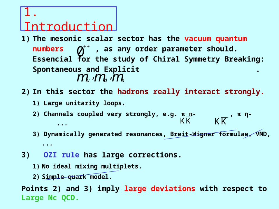
1) The mesonic scalar sector has the vacuum quantum numbers , as any order parameter should. Essencial for the study of Chiral Symmetry Breaking: Spontaneous and Explicit .

2) In this sector the hadrons really interact strongly.

1) Large unitarity loops.

2) Channels coupled very strongly, e.g. π π- , π η- ...

3) Dynamically generated resonances, Breit-Wigner formulae, VMD, ...

3) OZI rule has large corrections.

1) No ideal mixing multiplets.

2) Simple quark model.

Points 2) and 3) imply large deviations with respect to Large Nc QCD.

0

mmm sdu,,

KK KK

4) A precise knowledge of the scalar interactions of the lightest hadronic thresholds, π π and so on, is often required.– Final State Interactions (FSI) in ´/ , Pich, Palante,

Scimemi, Buras, Martinelli,...– Quark Masses (Scalar sum rules, Cabbibo suppressed Tau

decays.)– CKM matrix (Vus)– Fluctuations in order parameters of SSB. Stern et al.

5) Recent and accurate experimental data are bringing further evidence on the existence of the , (E791) and further constrains to the present models (CLOE).

6) The effective field theory of QCD at low energies is Chiral Perturbation Theory (CHPT).

This allows a systematic treatment of pion physics, but only cose to threshold, .( < 0.4-0.5 GeV)s

Chiral Perturbation TheoryWeinberg, Physica A96,32 (79); Gasser, Leutwyler, Ann.Phys. (NY) 158,142 (84)

QCD Lagrangian Hilbert Space Physical States

u, d, s massless quarks Spontaneous Chiral Symmetry Breaking SU(3)L SU(3)R SU(3)V



u, d, s massless quarks Spontaneous Chiral Symmetry Breaking SU(3)L SU(3)R

Goldstone Theorem Octet of massles

pseudoscalars π, K, η

Energy gap , *, , 0*(1450)

mq 0. Explicit breaking Non-zero massesof Chiral Symmetry mP

2 mq

SU(3)V

CHPT

π, K, η



u, d, s massless quarks Spontaneous Chiral Symmetry Breaking SU(3)L SU(3)R

Goldstone Theorem Octet of massles

pseudoscalars π, K, η

Energy gap , *, , 0*(1450)

mq 0. Explicit breaking Non-zero massesof Chiral Symmetry mP

2 mq

Perturbative expansion in powers of the external four-momenta of the pseudo-Goldstone bosons over

SU(3)V

CHPT

...42 LLL )2CHPT

2(

2

4

pO

LL MGeV1CHPT

π, K, η

GeV14 f

2CHPT

• New scales or numerical enhancements can appear that makes definitively smaller the overall scale Λ, e.g:– Scalar Sector (S-waves) of meson-meson interactions with I=0,1,1/2 the unitarity loops are

enhanced by numerical factors.

– Presence of large masses compared with the typical momenta, e.g. Kaon masses in driving the appearance of the Λ(1405) close to tresholed. This also occurs similarly in the S-waves of Nucleon-Nucleon scattering.

s 4mπ2

6f2 s mπ

2

f2

P-WAVE S-WAVE

Enhancement by factors 6L

Let us keep track of the kaon mass, MeV

We follow similar argumentos to those of S. Weinberg in NPB363,3 (´91)

respect to NN scattering (nucleon mass).

500KM

Unitarity Diagram

dq0

( )k0 q0 iε + ( )q0 E( )q + iε ( )q0 E( )q iε +

1

k0 E( )q

1

2E( )q 2MK

k2 q2

1

2MK

Unitarity enhancement for low three-momenta: 2MK

q

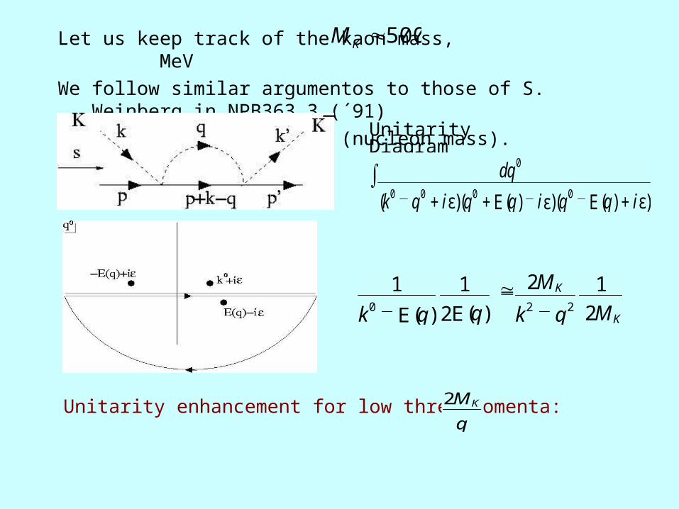
Let us keep track of the kaon mass, MeV

We follow similar argumentos to those of S. Weinberg in NPB363,3 (´91)

respect to NN scattering (nucleon mass).

500KM

Unitarity Diagram

dq0

( )k0 q0 iε + ( )q0 E( )q + iε ( )q0 E( )q iε +

1

k0 E( )q

1

2E( )q 2MK

k2 q2

1

2MK

Unitarity enhancement for low three-momenta: 2MK

q

This enhancement takes place in the real part of the uniarity

bubble: Analyticity

1

M2 q2 =1

q2

q2

M4 + q4

M6 + ... q2 + < < M2

Resonances give rise to a resummation of the chiral series at the

tree level (local counterterms beyond O( ).

The counting used to perform the matching is a simultaneous one in the number of loops calculated at a given order in CHPT (that increases order by

order). E.g:– Meissner, J.A.O, NPA673,311 (´00) the πN scattering was

studied up to one loop calculated at O( ) in HBCHPT+Resonances.

CHPT+Resonances

Ecker, Gasser, Pich and de Rafael, NPB321, 311 (´98)

4p

3p

1. A systematic scheme able to be applied when the interactions between the hadrons are not perturbative (even at low energies).• S-wave meson-meson scattering: I=0 (σ(500), f0(980)), I=1 (a0(980)),

I=1/2 ((700)). Related by SU(3) symmetry.

• S-wave Strangeness S=-1 meson-baryon interactions. I=0 Λ(1405) and other resonances.

• 1S0, 3S1 S-wave Nucleon-Nucleon interactions.

2. Then one can study:– Strongly interacting coupled channels.

– Large unitarity loops.

– Resonances.

3. This allows as well to use the Chiral Lagrangians for higher energies.4. The same scheme can be applied to productions mechanisms. Some

examples:• Photoproduction:

• Decays:

2. The Chiral Unitary Approach

KKKK00 0 ,, ,,

/ J 000 ,, KK

• Above threshold and on the real axis (physical region), a partial wave amplitude must fulfill because of unitarity:

General Expression for a Partial Wave Amplitude

ImT ij =k T ik ρk Tkj* ImT 1

ij= ρ i δ ijUnitarity Cut

W=s

We perform a dispersion relation for the inverse of the partial wave (the unitarity cut is known)

T ij1=R ij

1 δ ij g( )s0 i

s s0

π ρ( )s´ ids´

( )s´ s i0+ ( )s´ s0

+

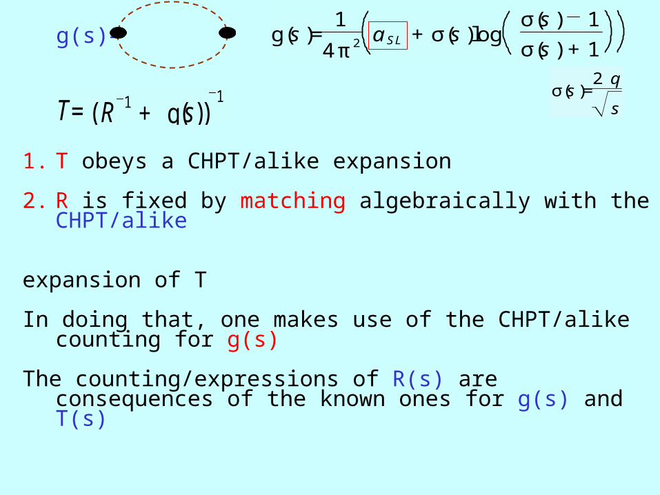
The restg(s): Single unitarity bubble

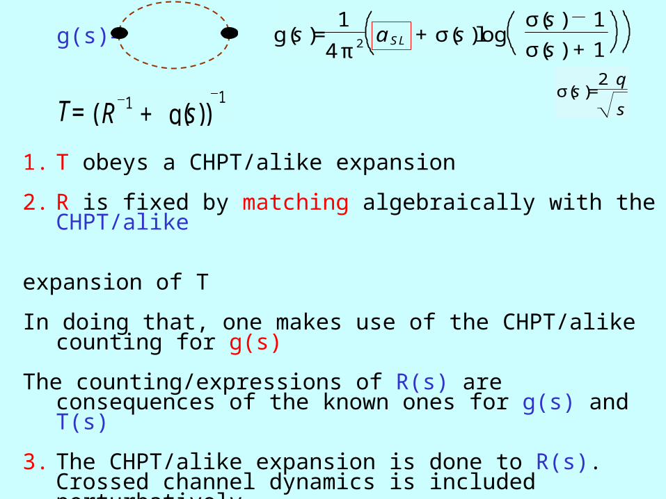
g(s)= g( )s =1

4π 2aSL σ( )s log

σ( )s 1

σ( )s 1 + +

σ( )s =2 q

sT= ( )R 1 g( )s + 1

g(s)= g( )s =1

4π 2aSL σ( )s log

σ( )s 1

σ( )s 1 + +

σ( )s =2 q

sT= ( )R 1 g( )s + 1

1. T obeys a CHPT/alike expansion

g(s)= g( )s =1

4π 2aSL σ( )s log

σ( )s 1

σ( )s 1 + +

σ( )s =2 q

sT= ( )R 1 g( )s + 1


2. R is fixed by matching algebraically with the CHPT/alike

expansion of T

In doing that, one makes use of the CHPT/alike counting for g(s)

The counting/expressions of R(s) are consequences of the known ones for g(s) and T(s)

g(s)= g( )s =1

4π 2aSL σ( )s log

σ( )s 1

σ( )s 1 + +

σ( )s =2 q

sT= ( )R 1 g( )s + 1



expansion of T



3. The CHPT/alike expansion is done to R(s). Crossed channel dynamics is included perturbatively.

g(s)= g( )s =1

4π 2aSL σ( )s log

σ( )s 1

σ( )s 1 + +

σ( )s =2 q

sT= ( )R 1 g( )s + 1



expansion of T



3. The CHPT/alike expansion is done to R(s). Crossed channel dynamics is included perturbatively.

4. The final expressions fulfill unitarity to all orders since R is real in the physical region (T from CHPT fulfills unitarity pertubatively as employed in the matching).

The re-scattering is due to the strong ``final´´ state interactions from some ``weak´´ production mechanism.

Production Processes

ImFi =k Fk ρk Tki*

We first consider the case with only the right hand cut for the strong interacting amplitude, is then a sum of poles (CDD) and a constant. It can be easily shown then:

1R

F=( )I Rg( )s + 1ξ

Finally, ξ is also expanded pertubatively (in the same way as R) by the matching process with CHPT/alike expressions for F, order by order. The crossed dynamics, as well for the production mechanism, are then included pertubatively.

Finally, ξ is also expanded pertubatively (in the same way as R) by the matching process with CHPT/alike expressions for F, order by order. The crossed dynamics, as well for the production mechanism, are then included pertubatively.

Meson-Meson Scalar Sector

T= ( )R 1 g( )s + 1

T=T2=R2 R2gR2 .. +

g is order 1 in CHPT

R=R2=T2

Let us apply the chiral unitary approach

LEADING ORDER:

Oset, J.A.O, NPA620,438(´97)

I=0

I=1

ππ, KŪUK A three-momentum cut-off was used in the calculation

of g(s). The only free parameter.πη 8 , KŪUK

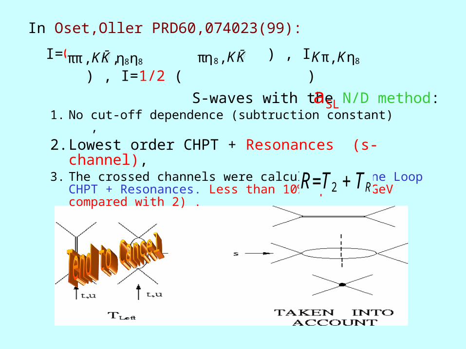
In Oset,Oller PRD60,074023(99):

I=0 ( ) , I=1 ( ) , I=1/2 ( )

S-waves with the N/D method:1. No cut-off dependence (subtruction constant) ,

2. Lowest order CHPT + Resonances (s-channel),3. The crossed channels were calculated in One Loop CHPT +

Resonances. Less than 10% up to 1 GeV compared with 2) .

aSL

ππ , KŪUK ,η8η8 πη 8 , KŪUK Kπ, Kη8

R=T2 TR +

I=1

I=0

I=1/2

f0(980)f0(500)

a0(980)

(800)

I=0

I=0

Kπ, Kη8ππ , KŪUK ,η8η8 πη 8 , KŪUKSolid lines: I=0 ( ) , I=1 ( ) , I=1/2 ( )

Singlet 1 GeV:

Octet 1.4 GeV:

Subtraction Constant: a=-0.750.20

ãac d=20.9MeV ; ãac m=10.6MeV; M1=1021MeV

cd=19.1MeV ; cm=1530MeV; M8=1390MeV

Dashed lines: I=0 ( ) , I=1 ( ) , I=1/2 ( )

No bare Resonances

Subtraction Constant: a=-1.23

ππ , KŪUK ,η8η8 Kπ, Kη8

Short-Dashed lines: I=0 ( ) , I=1 ( ) , I=1/2 ( )

No bare Resonances

Several Subtraction Constants:

ππ, KŪUK πη 8 , KŪUK

πη 8 , KŪUK

Kπ, Kη8

aππ = 1.14; aKŪUK = 1.64; aπη = 0.5; aKπ= 0.75; aKη= 0.75

Dynamically generated resonances.

TABLE 1Spectroscopy:

** Unitarity Normalization for , , extra 1/2 factor

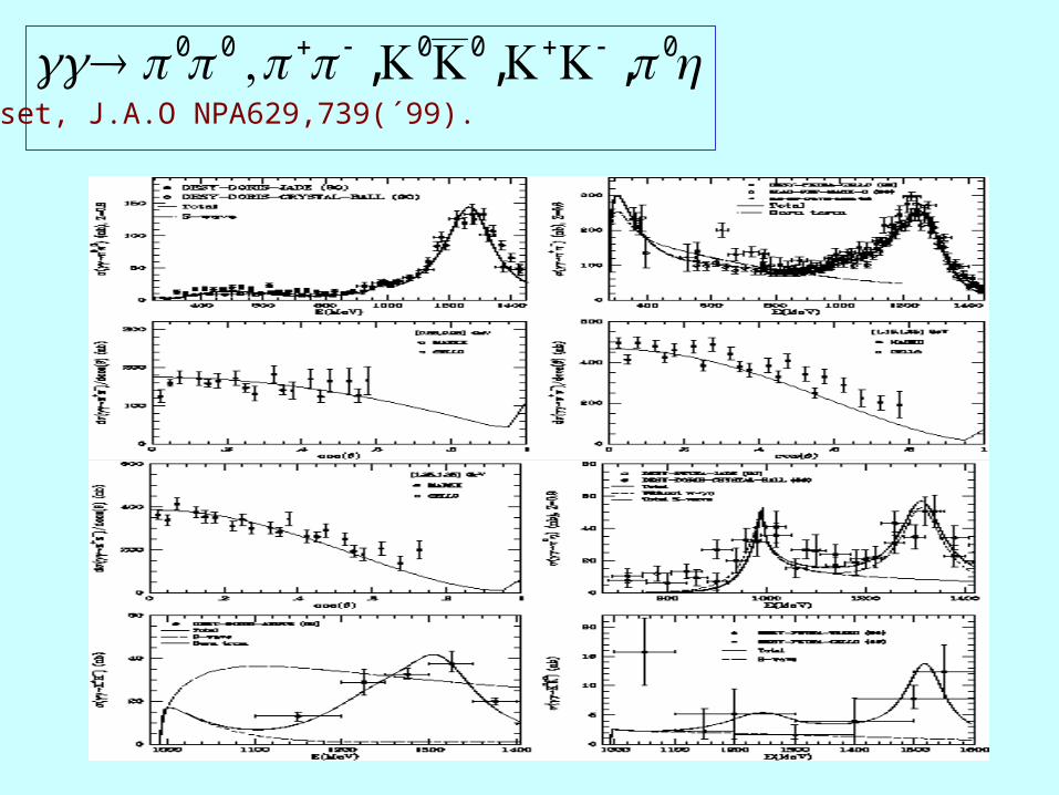
00000 ,,, Oset, J.A.O NPA629,739(´99).

/ JMeissner, J.A.O NPA679,671(´01).

Oset, Li, Vacas nucl-th/0305041 J/ decays to N anti-N meson-meson

J.A.O. NPA714, 161 (´02)

Oset, Palomar, Roca, Vacas hep-ph/0306249

000 ,, KKBS: 0=- 1= +180.83 MeV,

G0= G1=1.42/162 .

IAM: 0=- 1= +146.42 MeV,

G0= G1=1.54/162 .

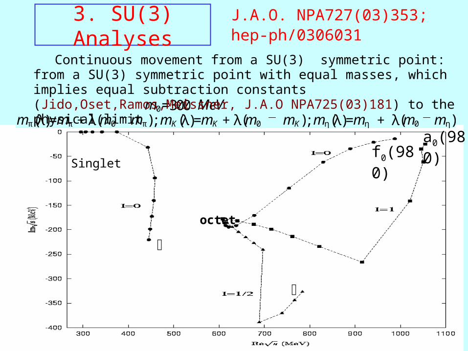
mπ( )λ =mπ λ( )m0 mπ ; mK( )λ + =mK λ( )m0 mK ; mη( )λ + =mη λ( )m0 mη + m0=300 MeV

3. SU(3) Analyses

Continuous movement from a SU(3) symmetric point: from a SU(3) symmetric point with equal masses, which implies equal subtraction constants (Jido,Oset,Ramos,Meissner, J.A.O NPA725(03)181) to the physical limit

octet

Singlet

a0(980)f0(980)

J.A.O. NPA727(03)353; hep-ph/0306031

a0(980), : Pure Octet States

g( )a0 πη 8 =

1

5g8g( )a0

KŪUK 1 =3

10g8

g( )κKπ =3

20g8

g( )κKη8 =1

20g8

g( )a0KŪUK 1 , g( )a0

πη 8 , g( )κKπ12

From we calculate:

GeV 3.17.8|| 8 g

g( )a0 πη 8

g( )a0 KŪUK 1

= 0.82

g( )a0 KŪUK 1

g( )κ Kπ12

= 0.82

g( )κ Kπ12

g( )κ Kη8

= 30.700.04 1.640.05 from table 1

2.50.25 from Jamin,Pich,J.A.O NPB587(00)331

1.100.03

This is an indication that systematic errors are larger than really shown in table 1 from the 3 T-matrices

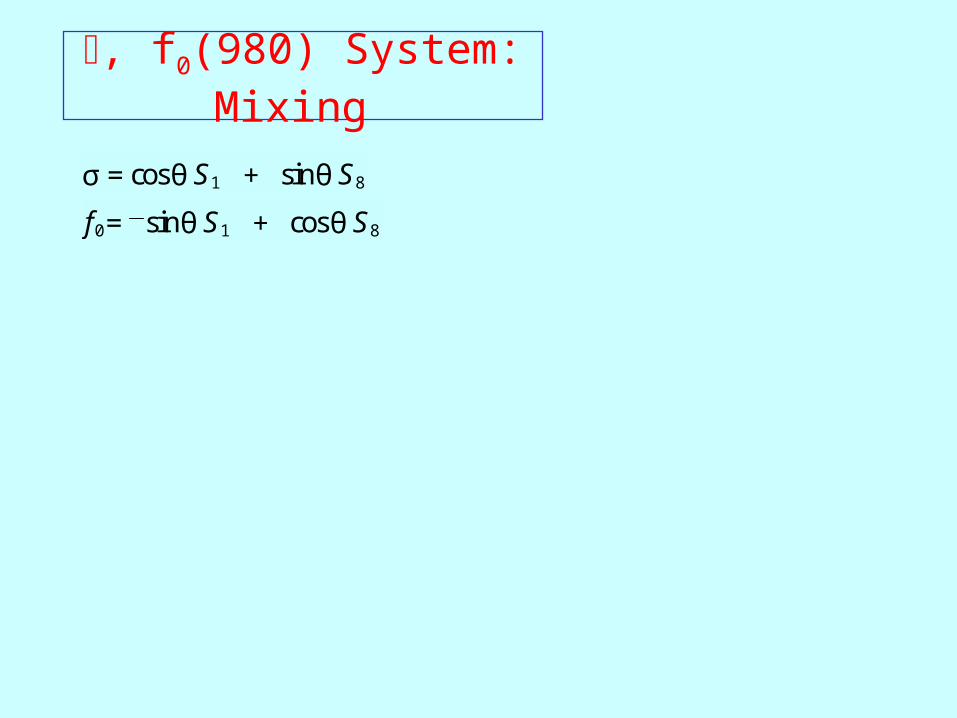
, f0(980) System: Mixing

f0= sinθ S1 cos θ S8 +

σ = cos θ S1 sinθ S8 +

, f0(980) System: Mixing

f0= sinθ S1 cos θ S8 +

σ = cos θ S1 sinθ S8 + Ideal Mixing: cos 2θ =

2

3= 0.67

Morgan, PLB51,71(´74); f0(980), a0(980), (1200), f0(1100) cos2 = 0.13

Jaffe, PRD15,267(´77); f0(980), a0(980), (900), f0(700) cos2 = 0.33

Dual Ideal Mixing

Scadron, PRD26,239(´82); f0(980), a0(980), (800), f0(750) cos2 = 0.39

Napsuciale (hep-ph/9803396),+ Rodriguez Int.J.Mod.Phys.A16,3011(´01);

f0(980), a0(980), (900), f0(500) cos2 = 0.87

Black, Fariborz, Sannino, Schechter PRD59,074026(´99) (Syracuse group);

f0(980), a0(980), (800), f0(600) cos2 = 0.63

σ =ūuu u ŪUd d +

2; f0( )980 = ūussqq If

Standard Unitary Symmetry Model analysis in vector and tensor nonets of coupling constants.Okubo, PL5,165(´63)

Glashow,Socolow,PRL15,329(´65)

g( 8 8)=0

g1

g8

=8

5tan θ

g( )σ ππ 0

g8

= 23

10sin θ

g( )f0 KŪUK 0

g8

=1

10cos θ ( )1 2 tan2θ +

|g8 | = 10.5 0.5 GeVcos 2 θ = 0.93 0.01|θ| =(14.9 0.8)°

STRATEGY I: We take the most important couplings for the and f0(980) to determining g8 and

STRATEGY II: We take the 6 ratios between the and f0(980) couplings to determining tan

)/( ; )/( ; )/(

)/( ; )/( ; )/(

000

000

fKKKKfKKfKK

fKKff

gggggg

gggggg11 12

21

13

22 23

We generate 12 numbers: calculating tan for the maximum and minimum values of ij from table 1

λ11=2 tanθ

tan2θ 1and so on

11 0.75 0.65

12 0.28 0.25

13 0.38 0.33

21 0.83 0.71

22 0.71 0.36

23 1.00 0.46

tan

tan=0.560.25

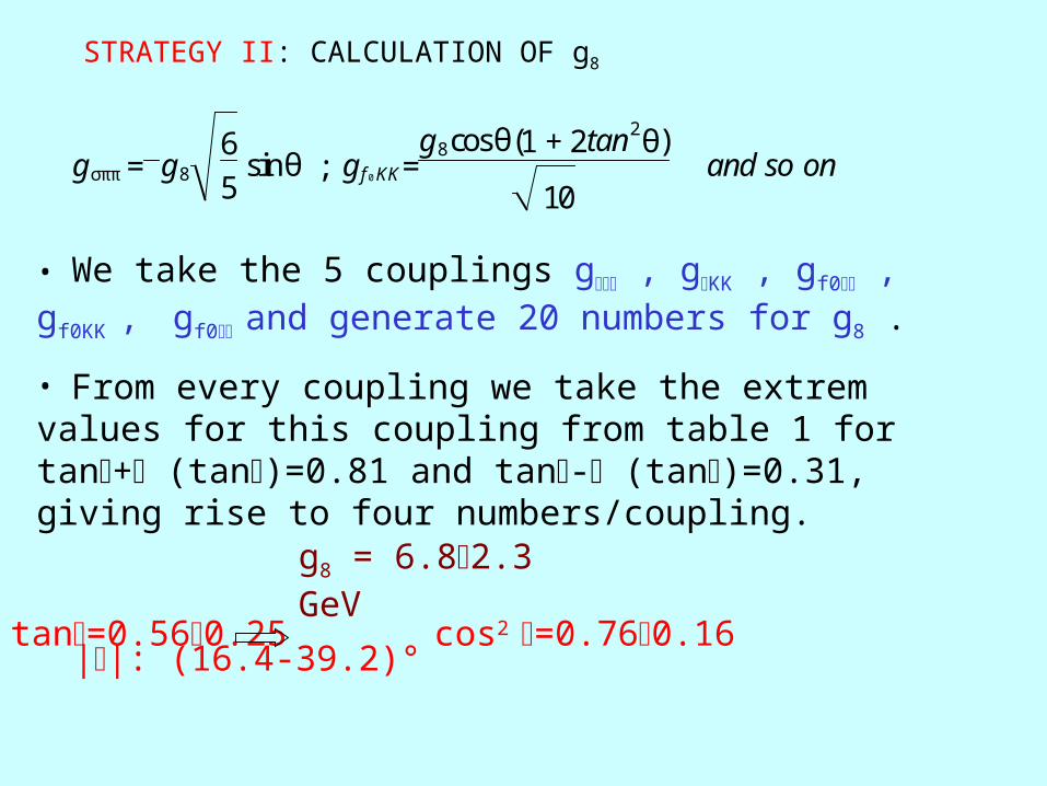
STRATEGY II: CALCULATION OF g8

• We take the 5 couplings g , gKK , gf0 , gf0KK , gf0 and generate 20 numbers for g8 .

• From every coupling we take the extrem values for this coupling from table 1 for tan+ (tan)=0.81 and tan- (tan)=0.31, giving rise to four numbers/coupling.

gσππ = g8

6

5sinθ ; g f 0 KK=

g8cos θ( )1 2tan2θ +

10and so on

g8 = 6.82.3 GeV

tan=0.560.25 cos2 =0.760.16 ||: (16.4-39.2)°

III.2) We take the same error for all the couplings g(RPQ) such that 2

dof =1 .

tan = 0.59 0.15 cos2 = 0.86 0.13

g8 = ( 7.7 0.8 ) GeV

STRATEGY III: 2 calculation between the couplings in the table and those predicted by SU(3)

χ2 = R=( )σ f 0 PQ

( )|g( )R PQ | |g( )R PQ SU( )3 | 2

σR,PQ2

III.1) We multiply the error obtained from table 1 for each coupling g(RPQ) by a common factor so that 2

dof =1 .

tan = 0.35 0.10 cos2 = 0.89 0.06

g8 = ( 8.2 0.8 ) GeV

III.2) We take the same error for all the couplings gRPQ such that 2

dof =1 .

tan = 0.59 0.15 cos2 = 0.86 0.13

g8 = ( 7.7 0.8 ) GeV

III.1) We multiply the error obtained from table 1 for each coupling gRPQ by a common factor so that 2

dof =1 .

tan = 0.35 0.10 cos2 = 0.89 0.06

g8 = ( 8.2 0.8 ) GeV

III.3) Error[gRPQ]={(0.2 gRPQ)2+2} and is fixed such that 2dof

=1 .

tan = 0.67 0.15 cos2 = 0.69 0.10

g8 = ( 7.0 0.8 ) GeV

I: g , gf0KK g8=10.50.5 GeV cos2=0.930.06

II: All couplings g8=6.82.3 GeV cos2=0.760.16

III: Fit,

multiplying errors

g8=8.20.8 GeV cos2=0.890.06

III: Fit, Global

error

g8=7.70.8 GeV cos2=0.740.10

III: Fit, 20% +

systematic error

g8=7.00.8 GeV cos2=0.690.10

From a0(980), g8=8.71.3 GeV

Paper

We average by taking the extrem values from each entry x+(x) and x- (x) 12 numbers g8

10 numbers cos2

g8 = 8.21.8 GeV

cos2=0.800.15

||: (13-34.4)° g1 = 4.692.7 GeV

I: g , gf0KK g8=10.50.5 GeV cos2=0.930.06

II: All couplings g8=6.82.3 GeV cos2=0.760.16

III: Fit,

multiplying errors

g8=8.20.8 GeV cos2=0.890.06

III: Fit, Global

error

g8=7.70.8 GeV cos2=0.740.10

III: Fit, 20% +

systematic error

g8=7.00.8 GeV cos2=0.690.10

From a0(980), g8=8.71.3 GeV

Paper

g8 = 8.21.8 GeV 21%

cos2=0.800.15 18%

||: (13-34.4)°

We average the extrem values for g8 and cos2

g8 = 83 GeV (37%)

cos2=0.80.2 (0.25%)

||: (0-39)°

g=2.94-3.01gKK=1.09-1.30g=0.04-0.09

g=3.61.5gKK=1.00.4g=0

g=3.02.5gKK=0.90.7g=0.

f0(980)gf0=0.89-1.33gf0KK=3.59-3.83gf0=2.61-2.85

gf0=3.01.1gf0KK=3.40.8gf0=2.90.6

gf0=3.11.7gf0KK=3.31.3gf0=2.80.9

a0(980)ga0=3.67-4.08ga0KK=5.39-5.60

ga0=3.71.4ga0KK=4.51.4

ga0=3.61.9ga0KK=4.42.3

gK=4.89-5.02g K=2.96-3.10 1.1-2.1

gK=5.51.7g K=1.80.6

gK=5.42.8g K=1.81.0

g=2.94-3.01gKK=1.09-1.30g=0.04-0.09

g=4.0 1.4gKK=1.20.4g=0.

g=3.61.5gKK=1.00.4g=0

g=3.02.5gKK=0.90.7g=0.

f0(980)gf0=0.89-1.33gf0KK=3.59-3.83gf0=2.61-2.85

gf0=2.41.1gf0KK=3.50.9gf0=2.810.6

gf0=3.01.1gf0KK=3.40.8gf0=2.90.6

gf0=3.11.7gf0KK=3.31.3gf0=2.80.9

a0(980)ga0=3.67-4.08ga0KK=5.39-5.60

ga0=3.41.1ga0KK=4.221.1

ga0=3.71.4ga0KK=4.51.4

ga0=3.61.9ga0KK=4.42.3

gK=4.7-5.02g K=2.96-3.10 1.1-2.1

gK=5.21.6g K=1.70.5

gK=5.51.7g K=1.80.6

gK=5.42.8g K=1.81.0

We remove the values from Strategy I (higher than the rest)

A)g8=7.71.7 22% , cos2=0.760.15 20%, ||: (17-39)°

B) g8 = 8.21.8 GeV 21% cos2=0.800.15 18% : (13-34.4)°

Second SU(3) Analysis: Couplings of the resonances with SU(3) two pseudosclar eigenstates.

Second SU(3) Analysis: Couplings of the resonances with SU(3) two pseudosclar eigenstates.

Averaging a0(980), couplings: GeV 5.05.8|| 8 g

Second SU(3) Analysis: Couplings of the resonances with the SU(3) two pseudosclar eigenstates.

Averaging a0(980), couplings: GeV 5.05.8|| 8 g

A) g( 1)= g1 cos = 4.71.7

g( 8)= g8 sin = 3.61.3

g( f01)=- g1 sin = 2.51.2

g( f08)= g8 cos = 6.61.5

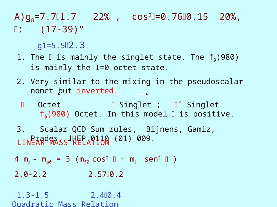
A)g8=7.71.7 22% , cos2=0.760.15 20%, : (17-39)°

g1=5.52.3

1. The is mainly the singlet state. The f0(980) is mainly the I=0 octet state.

2. Very similar to the mixing in the pseudoscalar nonet but inverted.

Octet Singlet ; ´ Singlet f0(980) Octet. In this model is positive.

3. Scalar QCD Sum rules, Bijnens, Gamiz, Prades, JHEP 0110 (01) 009.

LINEAR MASS RELATION

4 m - ma0 = 3 (mf0 cos2 + m sen2 )

2.0-2.2 2.570.2

1.3-1.5 2.40.4 Quadratic Mass Relation

Sign of Non-strange, strange basis: s=V3

3ns=1

2V1

1 V22 +

Γ2s

Γ2ūunn =5.5

At the f0(980) peak. Clearly the f0(980) should be mainly strange and then >0

Scalar Form Factors I=0

U.-G. Meissner, J.A.O NPA679(00)671

<0|ūus s| f0>

<0|ūunn|f 0 >

=

sinθ ycos θ

3 +

sinθ y

3cos θ +

y =<0|s1 |S1>

<0|s8 |S8> 1 in U( )3 symmetry

A) >0 ratio= 5.03 <0 ratio= 0.30.2

4. Conclusions

1. f0(980), a0(980), (900), f0(600) or form the lightest scalar nonet.

2. They evolve continuously from the physical situation to a SU(3) symmetric limit and give rise to a degenerate octet of poles and a singlet pole.

3. Several different SU(3) analyses of the scalar resonance couplings constants. They are consistent among them within 20%.

4. cos2=0.770.15; =28 11; is mainly a singlet and the f0(980) is

mainly the I=0 octet state.

5. These scalar resonances satisfy a Linear Mass Relation.

6. The value of the mixing angle is compatible with the one of the

Syracuse group, ideal mixing, of the U(3)xU(3) with UA(1) breaking

model of Napsuciale from the U(2)xU(2) model of t´Hooft.

José A. Oller Univ. Murcia, Spain The Mixing Angle of the Lightest Scalar Nonet José A. Oller...

Documents

Transcript of José A. Oller Univ. Murcia, Spain The Mixing Angle of the Lightest Scalar Nonet José A. Oller...