Jointly Gaussian Random Variables - University of Waterlooece411/Slides_files/topic2.pdf · A few...
34
@G.Gong 1 Chapter 2. Review of Random Processes 1 Random Variables and Error Functions 2 Concepts of Random Processes 3 Wide-sense Stationary Processes and Transmission over LTI 4 White Gaussian Noise Processes
Transcript of Jointly Gaussian Random Variables - University of Waterlooece411/Slides_files/topic2.pdf · A few...

@G.Gong 1
Chapter 2. Review of Random ProcessesChapter 2. Review of Random Processes
1 Random Variables and Error Functions2 Concepts of Random Processes3 Wide-sense Stationary Processes and
Transmission over LTI4 White Gaussian Noise Processes

Means, Variances, and moments of Random VariablesMeans, Variances, and moments of Random Variables
Let X be a random variable with the density function fX(x).Mean of X
Variance of X
The second of moment of X
Relationship
If X is a discrete random variable, then the above integrals are replaced by the summations.
∫∞
∞−
== dxxxfXE X )(][μ
])[(][ 22 μσ −== XEXVar ∫∞
∞−
−= dxxfx X )()( 2μ
∫∞
∞−
== dxxfxXEm X )(][ 22
22 μσ −= m
1 Random Variables and Error Functions

Correlation andCovariance
Correlation andCovariance
Let X and Y be two random variables, fX,Y(x, y) be their joint density function,
, ,their respective means,
, variances, and Z = g(X, Y)is well-defined. Then Z is also a random variable, and the mean ofZ is given by
∫∞
∞−
= dxyxfyxgYXgE YX ),(),()],([ ,
If , then
is the correlation of X and Y. If , then
is the covariance of X and Y. If then
is the correlation coefficient.Relationship:
XYYXg =),(
][XEX =μ ][YEY =μ
][)],([ XYEYXgE =
))((),( YX YXYXg μμ −−=
)])([( )],([),(
YX YXEYXgEYXCov
μμ −−==
)/())((),( YXYX YXYXg σσμμ −−=][2 XVarX =σ ][2 YVarY =σ
)],([),( YXgEYX =ρ
YX
YXCovYXσσ
ρ ),(),( =
If ρ = 0, then X and Y are said to be uncorrelated.

t μ
σπ21
f(t)
Unit or standard gaussian: μ = 0 and σ = 1. The cdf of the unit gaussian:
∫∞−
−=Φx
t dtex 2/2
21)(π
x t
f(t)
Φ(x) = the shaded area
μ = 0, σ = 1
X ∼ N(μ, σ): X is a gaunssian r.v. with mean μ and variance σ. The pdf of X:
The cdf of X:
∞<<∞−=−
−tetf
t
,21)( 2
2
2)(
σμ
σπ
∫∞−
=x
dttfxF )()(
⎟⎠⎞
⎜⎝⎛ −
Φ=σμxxF )(
Computation of F(x):
Guassian Random Variables

Jointly Gaussian Random VariablesJointly Gaussian Random Variables
Let X and Y be gaussian random variables with means μX and μy, variances σX and σy. We say that X and Y have a bivariate Gaussian pdfif the joint pdf of X and Y is given by
⎥⎥⎦
⎤
⎢⎢⎣
⎡
−−
−= Syxf
YXYX )1(2
1exp12
1),( 22, ρρσπσ
where
YX
YX
Y
Y
X
X yxyxSσσ
μμρ
σμ
σμ ))((2
22−−
−⎟⎟⎠
⎞⎜⎜⎝
⎛ −+⎟⎟
⎠
⎞⎜⎜⎝
⎛ −=

Property. If is defined by the above, then the conditional distributions of X given that Y = y, and Y given that X = x, respectively, are all gaussian distributions with the following parameters listed in (a).
),(, yxf YX
YX
YXCovYXσσ
ρρ ),(),( ==
(b) The parameter ρ is equal to the correlation coefficient of Xand Y, i.e.,
(c) X and Y are independent if and only if X and Y are uncorrelated. In other word, X and Y are independent if and only if ρ = 0.
)()(~Y
Y
XXX yy μ
σσρμμ −+=
)1(~ 222 ρσσ −= XX
)|(| yYxf YX =
)~),(~( 2XX yN σμ
where
(a) :
What are the parameters of
?)|(| xXyf XY =

Q(x) FunctionQ(x) Function
The cdf of the unit Gaussian random variable , reproduced here:
∫∞−
−=Φx
t dtex 2/2
21)(π
x t
f(t)
Φ(x) = the shaded area
x t
f(t)
Q(x) = the shaded area
Q(x) function is defined by
Q(x) = 1 – Φ(x)
which is called the tail probability.

The error function:
Relation:
∫ −=x
t dtexerf0
22)(π
∫∞
−=x
t dtexerfc22)(
π
What are the relationships among Φ(x), Q(x), erfc(x), or erf(x)?
⎟⎠
⎞⎜⎝
⎛=22
1)( xerfcxQ
⎟⎟⎠
⎞⎜⎜⎝
⎛−=Φ
2211)( xerfcx
⎟⎟⎠
⎞⎜⎜⎝
⎛+=
221
21 xerf
⎟⎟⎠
⎞⎜⎜⎝
⎛ −+=
σμ
221
21)( xerfxF
Error Function and the Complementary Error Function Error Function and the Complementary Error Function
)(1 xerferfc −=
X is a gaunssian r.v. with mean μ and variance σ, then the cdf F(x) of X can be expressed in terms of erf(x):
The complementary error function:

A few remarks on the definition of random processes:A few remarks on the definition of random processes:
A random process is a collection of random variables:
{X(t), t∈ T}where X(t) is a random variable which maps an outcome ξ to a number
X(t, ξ) for every outcome of an experiment. We will use X(t) to represent a random process omitting , as in the case of random variables, its dependence on ξ.
X(t) has the following interpretations:
It is a single time function (or a sample function, the realization of the process).
Both t and ξ are variables
It is a family (or ensemble) of functions X(t, ξ).
If t and ξ are fixed, then
X(t) is a random variable equal to the state of the given process at time t.
t is variable and ξ is fixed
t is fixed and ξ is variable
X(t) is a number
2 Concepts of Random Processes

@G.Gong 10
In a communication system, there are two types of random processes:In a communication system, there are two types of random processes:
The noise /interference introduced by channel is a random process.
For the transmitted signals, they have two properties:- the signals are functions of time- the signals are random in the sense that before conducting an
experiment, it is not possible to describe exactly the waveformthat will be observed.
Thus a transmitted signal is a random process.

@G.Gong 11
Example 2.1. Experiment: to transmit 3 binary digits to the receiver
1
T0
T: symbol duration
T
X(t) is a random process or a random signal which is a collection of all the following eight waveforms.
{ })(),....,( 70 tXtX

T 2T 3T000 X0(t)
001 X1(t)
010 X2(t)
011 X3(t)
0tt =
100 X4(t)
101 X5(t)
110 X6(t)
111 X7(t)
Sample functions

Example 2.2. The voltage of an ac generator with random amplitude A and phase Θ is given by
)2cos()( Θ+= tfAtX cπ
where Θ is a random variable uniformly distributed over (0, 2π).
X(t) is a random process which consists of a family of cosine waves and a single sample is the function:
)2cos(),( θπθ += tfAtX c
The following figures showed samples functions for θ being equal to 0, θ/2, -θ /4, and θ/4.

@G.Gong 14
−8 −6 −4 −2 0 2 4 6 8−1
−0.8
−0.6
−0.4
−0.2
0
0.2
0.4
0.6
0.8
1
−8 −6 −4 −2 0 2 4 6 8−1
−0.8
−0.6
−0.4
−0.2
0
0.2
0.4
0.6
0.8
1
−8 −6 −4 −2 0 2 4 6 8−1
−0.8
−0.6
−0.4
−0.2
0
0.2
0.4
0.6
0.8
1
θ = 0
θ = - π/4
θ = π/2
−8 −6 −4 −2 0 2 4 6 8−1
−0.8
−0.6
−0.4
−0.2
0
0.2
0.4
0.6
0.8
1
θ = π/4
t t
t t

@G.Gong 15
Difference between the two examplesDifference between the two examples
The first example consists of a family of functions that cannot be described in terms of a formula.
In the second example, the random process consists of a family of cosine waves and it is completely specified in terms of the random variable Θ.

Means, autocorrelation and crosscorrelationMeans, autocorrelation and crosscorrelation
Mean of the random process X(t) is the mean of random variable X(t) at time instant t:
where fX(t)(x) is the pdf of X(t) at time instant t.
∫+∞
∞−== dxxxftXEt tXX )()]([)( )(μ
Autocorrelation function of X(t) is a function of two variables t1 = t and t2 = t + τ,
)]()([),( ττ +=+ tXtXEttRXThis is a measure of the degree to which two time samples of the same random process are related.
Crosscorrelation function of two random processes X(t) abd Y(t) is a function of two variables t1 = t, and t2 = t + τ,, defined by
)]()([),(, ττ +=+ tYtXEttR YX

@G.Gong 17
)(),( )( ττ XX RttRii =+
What is a WSS Process?
In other words, a random process X(t) is WSS if its two statistics, its mean and autocorrelation, do not vary with a shift in the time origin.
3 Wide-Sense Stationary (WSS) Processes and Transmission over LTI
A process X(t) is WSS if the following conditions are satisfied:
independent of t.
depends only on the time difference τ and not on the variablest1 = t + τ. and t2 = t.
constant)]([)( )( == tXEti Xμ

Solution.
)]([ tXE
)2cos()( Θ+= tfAtX cπ
Example 2.3. Find the mean and autocorrelation function of the random process X(t) ( in E.g. 2.2),
⎩⎨⎧ ≤≤
=Θ otherwise ,020 ),2/(1
)(:pdfπθπ
θf
where Θ is uniformly distributed over [0, 2 π].
)])(2cos()2cos([ Θ++Θ+= τππ tfAtfAE cc
⎥⎦⎤
⎢⎣⎡ Θ+++= )2)2(2cos(
21)2cos(
212 τπτπ tffEA cc
)2cos(2
2τπ cf
A=
Since both the mean and autocorrelation of X(t) do not depend on time t, then X(t) is a WSS process.
= 0
),( τ+ttRX
θπ
θππ
dtfA c 21)2cos(
2
0∫ +=
Is X(t) a WSS?
According to the definitions,

@G.Gong 19
)()( 1. ττ −= XX RR
Properties of Autocorrelation Functionof a WSS process X(t)
Symmetric in τ about zero
)0()( .2 XX RR ≤τ for all τ, Maximum value occurred at the origin
)()( .3 fSR XX ↔τ Autocorrleation and psd form a pair of the Fourier transform
])([)0( 4. 2tXERX = The value at origin is equal to the average power of the signal

@G.Gong 20
Power Spectral Density (PSD) of a WSS Random Process
∫+∞
∞−
− == dfefSfSR fjXXX
τπτ 21 )())(()( F
))(()( τXX RfS F=
For a given WSS process X(t), the psd of X(t) is the Fourier transform of its autocorrelation, i.e.,
∫+∞
∞−
−= ττ τπ deR fjX
2)(

For the random process in Example 2.3, we have
Hence, the psd of X(t) is the Fourier transform of the autocorrelation of X(t), given by
)2cos(2
)(2
τπτ cX fAR =
[ ])()(4
)(2
ccX ffffAfS ++−= δδ
f
SX(f)A2/4A2/4
fc- fc

@G.Gong 22
)2cos()()( Θ+= tftXtY cπ
Example 2. 4 Let
where X(t) is a WSS process with psd SX(f), Θ is uniformly distributed over [0, 2 π], and X(t) is independent of Θ and
Find the psd of Y(t).
)2cos( Θ+tfcπ
Solution.
First we need to show that Y(t) is WSS.
)]([)( tYEtmY =
)]2cos()([ Θ+= tftXE cπ
(by independence )
)]2[cos()]([ Θ+= tfEtXE cπ
(by Example 2.3)
00)( =⋅= tmX
Mean:

)]()([ τ+= tYtYE
)])(2cos()()2cos()([ Θ+++Θ+= τπτπ tftXtftXE cc
)])(2cos()2[cos()]()([ Θ++Θ++= τππτ tftfEtXtXE cc
)2cos(21)( τπτ cX fR=
By Example 2.3.
Hence, Y(t) is WSS. Therefore
)( τYR=
)]([ )( τYY RFtS = )])(([41 22 τπτπτ cc fjfj
X eeRF −+=
[ ])()(41
cXcX ffSffS ++−=
),( ttRY τ+Autocorrelation of Y(t):

@G.Gong 24
Properties of PSDProperties of PSD
0)( 1. ≥fSX
)()( 2. fSfS XX −=
)()( .3 τXX RfS ↔
always real valued
for X(t) real-valued
a pair of Fourier transform
∫+∞
∞−== )()0( .4 dffSRP XX
Relationship between average power and psd

@G.Gong 25
Transmission over LTI SystemsTransmission over LTI Systems
Response of LTI system to a random input X(t):
h(t)X(t) Y(t)
)()()( thtXtY ∗=
τττ∫∞
∞−
−= dhtx )()(
3) Autocorrelation:
)()()()( ττττ −∗∗= hhRR XY
Properties of the output:
1) If X(t) is WSS, so does Y(t).
)0(HXY μμ =2) Mean:
4) PSD:
2|)(|)()( fHfSfS XY =

@G.Gong 26
h(t)X(t) Y(t)RX(τ) Ry(τ)
|H(f)|2 SY(f)SX(f)
F F-1

@G.Gong 27
4 White Gaussian Noise Processes4 White Gaussian Noise Processes
Definition. A random process N(t) is a white gaussian noise if N(t) is a WSS process satisfying
(1) (zero mean)(2) For any time instants t1 < t2 < … < tk, N(t1), N(t2), …, N(tk) are independent gaussian random variables.
0)]([ == tNENμ
1t 2t kt
)( ktN)( 2tN)( 1tN
@G.Gong 28
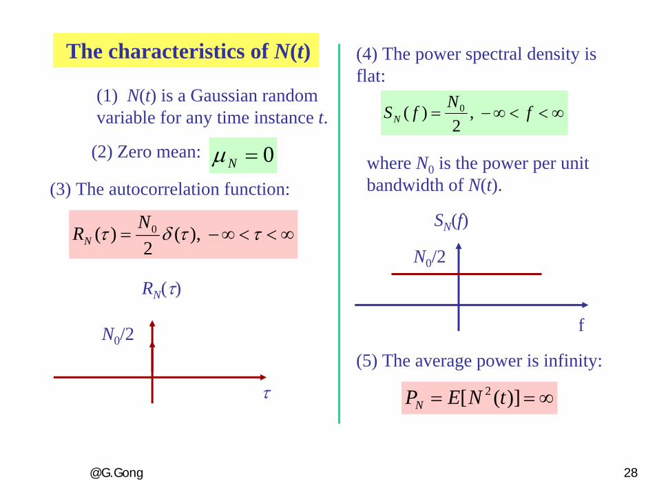
The characteristics of N(t)
(1) N(t) is a Gaussian random variable for any time instance t.
∞<<∞−= ττδτ ),(2
)( 0NRN
(3) The autocorrelation function: where N0 is the power per unit bandwidth of N(t).
∞<<∞−= fNfSN ,2
)( 0
(4) The power spectral density is flat:
f
SN(f)
N0/2
N0/2
τ
RN(τ)
0=Nμ(2) Zero mean:
(5) The average power is infinity:
∞== )]([ 2 tNEPN

@G.Gong 29
N0/2SN(f)
f
Power spectrum of thermal noise
The above spectrum achieves its maximum at f = 0. The spectrum goes to infinity, but the rate of convergence to zero is very slow. From this, we conclude that the thermal noise, though not precisely white, for all practical purpose can be modeled as a white gaussian noise process.

+
N(t)
X(t) Y(t) = X(t) + N(t)
Example 2. 5.Example 2. 5. Sum with a White Gaussian Noise.
Suppose that N(t) is a white Gaussian noise with power spectrum N0/2 . We also assume that X(t) and N(t) are joint WSS and independent. Find the mean and the power spectral density of Y(t).
Solution.Mean:
)]()([)( tNtXEtY +=μ)]([)]([ tNEtXE +=
XX μμ =+= 0
Autocorrelation:)]()([),( ττ +=+ tYtYEttRY
[ ]))()())(()(( ττ ++++= tNtXtNtXE),(),(),(),( ττττ tRtRtRtR NNXXNX +++=
(by independence and joint WSS)
)()()( τττ YNX RRR =+=
Thus, Y(t) is WSS. The psd of Y(t):
2)()()( 0NfSfSfS XNX +=+=
))()(())(()( τττ NXYY RRFRFfS +==

@G.Gong 31
Example 2.6 Effect of an Ideal Filter on White Gaussian Noise.
Find the psd and the autocorrelation of the output process Y(t). Is the output process Y(t) a white Gaussian noise ?
fc-fcf
H(f)
1
A white gaussian noise N(t) with psd is the input to the ideal low-pass filter shown below. 2
)( 0NfSN =

@G.Gong 32
Solution.
2|)(|)()( fHfSfS NY =
))(()( 1 fSFR YY−=τ
⎪⎩
⎪⎨⎧ ≤=
otherwise0
||for 2
0cffN
The autocorrelation is the inverse Fourier transform of the psd, thus
The psd is given by
)2(sin0 τcc fcfN=
Remark. The ideal low-pass filter transforms the autocorrelation (delta function) of white noise into a sinc function. After filtering, we no longer have white noise. The output signal will have zero correlation with shifted copies of itself, only at shifts of ( n not zero). )2/( cfn=τ

@G.Gong 33
Example 2.6 Effect of an RC Filter on White Gaussian Noise
⎩⎨⎧ ≥
=−
otherwise 00
)(te
that
A white gaussian noise N(t) with psd is the input to the RC filter with impulse response
where a = 1/(RC).
Find the psd and the autocorrelation of the output process Y(t).
2)( 0NfSN =

@G.Gong 34
Solution.
The frequency response is:
fjathFfH
π21))(()(
+== ⇒ 22
2
)2(1|)(|
fafH
π+=
Thus2|)(|)()( fHfSfS NY = 22
20
)2(2 faaNπ+
=
))(()( 1 fSFR YY−=τ RCeRCN /||0
4τ−=
Again, we no longer have white noise after filtering. The RC filter transforms the input autocorrelation function of white noise into an exponential function.


![ON THE COMPUTER GENERATION OF RANDOM ...luc.devroye.org/devroye_1982_computer_generation_random...Remarks On the computer generation of random convex hulls 3 1. [Validity]. When R,](https://static.fdocuments.in/doc/165x107/5fea5e498ade6850471db5bf/on-the-computer-generation-of-random-luc-remarks-on-the-computer-generation.jpg)


![Small Random Perturbations of Dynamical Systems and …ruelle/PUBLICATIONS/[65].pdf · Small Random Perturbations of Dynamical Systems and the Definition of Attractors David Ruelle](https://static.fdocuments.in/doc/165x107/5a9e3b927f8b9aee4a8ba77f/small-random-perturbations-of-dynamical-systems-and-ruellepublications65pdfsmall.jpg)