Joint Strategy Fictitious Play with Inertia for Potential Games∗

Jason R. Marden† Gurdal Arslan‡ Jeff S. Shamma§¶

October 28, 2005June 13, 2007 (revised)

Abstract

We consider multi-player repeated games involving a large number of players with large strategyspaces and enmeshed utility structures. In these “large-scale” games, players are inherently faced withlimitations in both their observational and computational capabilities. Accordingly, players in large-scale games need to make their decisions using algorithms that accommodate limitations in informationgathering and processing. This disqualifies some of the well known decision making models such as“Fictitious Play” (FP), in which each player must monitor the individual actions of every other playerand must optimize over a high dimensional probability space. We will show that Joint Strategy FictitiousPlay (JSFP), a close variant of FP, alleviates both the informational and computational burden of FP.Furthermore, we introduce JSFP with inertia, i.e., a probabilistic reluctance to change strategies, andestablish the convergence to a pure Nash equilibrium in all generalized ordinal potential games in bothcases of averaged or exponentially discounted historical data. We illustrate JSFP with inertia on thespecific class of congestion games, a subset of generalized ordinal potential games. In particular, weillustrate the main results on a distributed traffic routing problem and derive tolling procedures that canlead to optimized total traffic congestion.

1 Introduction

We consider “large-scale” repeated games involving a large number of players, each of whom selects a

strategy from a possibly large strategy set. A player’s reward, or utility, depends on the actions taken by

all players. The game is repeated over multiple stages, and this allows players to adapt their strategies in

response to the available information gathered over prior stages. This setup falls under the general subject

of “learning in games” [2, 3], and there are a variety of algorithms and accompanying analysis that examine

the long term behavior of these algorithms.

∗Research supported by NSF grants #CMS–0339228, #ECS–0501394, and #ECCS–0547692, and ARO grant #W911NF–04–1–0316. The conference version of this paper appears in [1].

†J. R. Marden is with the Department of Mechanical and Aerospace Engineering,University of California, 46-148 EngineeringIV, Los Angeles, CA 90095-1597,marden@seas.ucla.edu .

‡G. Arslan is with the Department of Electrical Engineering, University of Hawaii at Manoa, 440 Holmes Hall, 2540 DoleStreet, Honolulu, HI 96822,gurdal@hawaii.edu .

§J. S. Shamma is with the Department of Mechanical and Aerospace Engineering, University of California, 37-146 EngineeringIV, Los Angeles, CA 90095-1597,shamma@ucla.edu .

¶Corresponding author.

1

In large-scale games players are inherently faced with limitations in both their observational and com-

putational capabilities. Accordingly, players in such large-scale games need to make their decisions using

algorithms that accommodate limitations in information gathering and processing. This limits the feasibil-

ity of different learning algorithms. For example, the well-studied algorithm “Fictitious Play” (FP) requires

individual players to individually monitor the actions of other players and to optimize their strategies accord-

ing to a probability distribution function over the joint actions of other players. Clearly, such information

gathering and processing is not feasible in a large-scale game.

The main objective of this paper is to study a variant of FP called Joint Strategy Fictitious Play (JSFP)

[2, 4, 5]. We will argue that JSFP is a plausible decision making model for certain large-scale games. We

will introduce a modification of JSFP to include inertia, in which there is a probabilistic reluctance of any

player to change strategies. We will establish that JSFP with inertia converges to a pure Nash equilibrium for

a class of games known as generalized ordinal potential games, which includes so-called congestion games

as a special case [6].

Our motivating example for a large-scale congestion game is distributed traffic routing [7], in which

a large number of vehicles make daily routing decisions to optimize their own objectives in response to

their own observations. In this setting, observing and responding to the individual actions of all vehicles

on a daily basis would be a formidable task for any individual driver. A more realistic measurement on the

information tracked and processed by an individual driver is the daily aggregate congestion on the roads that

are of interest to that driver [8]. It turns out that JSFP accommodates such information aggregation.

We will now review some of the well known decision making models and discuss their limitations in

large-scale games. See the monographs [2, 9, 3, 10, 11] and survey article [12] for a more comprehensive

review.

The well known FP algorithm requires that each player views all other players as independent decision

makers [2]. In the FP framework, each player observes the decisions made by all other players and com-

putes the empirical frequencies (i.e. running averages) of these observed decisions. Then, each player best

responds to the empirical frequencies of other players’ decisions by first computing the expected utility for

each strategy choice under the assumption that the other players will independently make their decisions

2

probabilistically according to the observed empirical frequencies. FP is known to be convergent to a Nash

equilibrium in potential games, but need not converge for other classes of games. General convergence

issues are discussed in [13, 14, 15].

The paper [16] introduces a version of FP, called “sampled FP”, that seeks to avoid computing an ex-

pected utility based on the empirical frequencies, because for large scale games, this expected utility com-

putation can be prohibitively demanding. In sampled FP, each player selects samples from the strategy

space of every other player according to the empirical frequencies of that player’s past decisions. A player

then computes an average utility for each strategy choice based off of these samples. Each player still has

to observe the decisions made by all other players to compute the empirical frequencies of these observed

decisions. Sampled FP is proved to be convergent in identical interest games, but the number of samples

needed to guarantee convergence grows unboundedly.

There are convergent learning algorithms for a large class of coordination games called “weakly acyclic”

games [9]. In adaptive play [17] players have finite recall and respond to the recent history of other players.

Adaptive play requires each player to track the individual behavior of all other players for recall window

lengths greater than one. Thus, as the size of player memory grows, adaptive play suffers from the same

computational setback as FP.

It turns out that there is a strong similarity between the JSFP discussed herein and the regret matching

algorithm [18]. A player’s regret for a particular choice is defined as the difference between 1) the utility that

would have been received if that particular choice was played for all the previous stages and 2) the average

utility actually received in the previous stages. A player using the regret matching algorithm updates a

regret vector for each possible choice, and selects actions according to a probability proportional to positive

regret. In JSFP, a player chooses an action by myopically maximizing the anticipated utility based on

past observations, which is effectively equivalent to regret modulo a bias term. A current open question is

whether player choices would converge in coordination-type games when all players use the regret matching

algorithm (except for the special case of two-player games [19]). There are finite memory versions of the

regret matching algorithm and various generalizations [3], such as playing best or better responses to regret

over the lastm stages, that are proven to be convergent in weakly acyclic games when players use some

3

sort of inertia. These finite memory algorithms do not require each player to track the behavior of other

players individually. Rather, each player needs to remember the utilities actually received and the utilities

that could have been received in the lastm stages. In contrast, a player using JSFP best responds according

to accumulated experience over the entire history by using a simple recursion which can also incorporate

exponential discounting of the historical data.

There are also payoff based dynamics, where each player observes only the actual utilities received and

uses a Reinforcement Learning (RL) algorithm [20, 21] to make future choices. Convergence of player

choices when all players use an RL-like algorithm is proved for identical interest games [22, 23, 24] assum-

ing that learning takes place at multiple time scales. Finally, the payoff based dynamics with finite-memory

presented in [25] leads to a Pareto-optimal outcome in generic common interest games.

Regarding the distributed routing setting of Section 4, there are papers that analyze different routing

strategies in congestion games with “infinitesimal” players, i.e., a continuum of players as opposed to a

large, but finite, number of players. References [26, 27, 28] analyze the convergence properties of a class

of routing strategies that is a variation of the replicator dynamics in congestion games, also referred to as

symmetric games, under a variety of settings. Reference [29] analyzes the convergence properties of no-

regret algorithms in such congestion games and also considers congestion games with discrete players, as

considered in this paper, but the results hold only for a highly structured symmetric game.

The remainder of the paper is organized as follows. Section 2, sets up JSFP and goes on to establish

convergence to a pure Nash equilibrium for JSFP with inertia in all generalized ordinal potential games.

Section 3 presents a fading memory variant of JSFP, and likewise establishes convergence to a pure Nash

equilibrium. Section 4 presents an illustrative example for traffic congestion games. Section 4 goes on to

illustrate the use of tolls to achieve a socially optimal equilibrium and derives conditions for this equilibrium

to be unique. Finally, Section 5 presents some concluding remarks.

4

2 Joint Strategy Fictitious Play with Inertia

2.1 Setup

Consider a finite game withn-player setP := {P1, ...,Pn} where each playerPi ∈ P has an action setYi

and a utility functionUi : Y → R whereY = Y1 × ...× Yn.

Fory = (y1, y2, ..., yn) ∈ Y , let y−i denote the profile of player actionsother thanplayerPi, i.e.,

y−i = {y1, . . . , yi−1, yi+1, . . . , yn} .

With this notation, we will sometimes write a profiley of actions as(yi, y−i). Similarly, we may writeUi(y)

asUi(yi, y−i).

A profile y∗ ∈ Y of actions is called apure Nash equilibrium1 if, for all playersPi ∈ P,

Ui(y∗i , y∗−i) = max

yi∈Yi

Ui(yi, y∗−i). (1)

We will consider the class of games known as “generalized ordinal potential games”, defined as follows.

Definition 2.1 (Potential Games)A finite n-player game with action sets{Yi}ni=1 and utility functions

{Ui}ni=1 is apotential gameif, for some potential functionφ : Y1 × ...× Yn → R,

Ui(y′i, y−i)− Ui(y′′i , y−i) = φ(y′i, y−i)− φ(y′′i , y−i),

for every player, for everyy−i ∈ ×j 6=iYj and for everyy′i, y′′i ∈ Yi. It is a generalized ordinal potential

gameif, for some potential functionφ : Y1 × ...× Yn → R,

Ui(y′i, y−i)− Ui(y′′i , y−i) > 0 ⇒ φ(y′i, y−i)− φ(y′′i , y−i) > 0,

for every player, and for everyy−i ∈ ×j 6=iYj and for everyy′i, y′′i ∈ Yi.

In a repeatedversion of this setup, at every staget ∈ {0, 1, 2, ...}, each player,Pi, selects an action

yi(t) ∈ Yi. This selection is a function of the information available to playerPi up to staget. Both the

action selection function and the available information depend on the underlying learning process.

1We will henceforth refer to a pure Nash equilibrium simply as an equilibrium.

5

2.2 Fictitious Play

We start with the well known Fictitious Play (FP) process [2].

Define theempirical frequency, qyii (t), as the percentage of stages at which playerPi has chosen the

actionyi ∈ Yi up to timet− 1, i.e.,

qyii (t) :=

1t

t−1∑τ=0

I{yi(τ) = yi},

whereyi(k) ∈ Yi is playerPi’s action at timek andI{·} is the indicator function. Now define the empirical

frequency vector for playerPi as

qi(t) :=

qy1i...

qy|Yi|i

,

where|Yi| is the cardinality of the action setYi.

The action of playerPi at timet is based on the (incorrect) presumption that other players are playing

randomlyandindependentlyaccording to their empirical frequencies. Under this presumption, the expected

utility for the actionyi ∈ Yi is

Ui(yi, q−i(t)) :=∑

y−i∈Y−i

Ui(yi, y−i)∏

yj∈y−i

qyj

j (t), (2)

whereq−i(t) := {q1(t), ..., qi−1(t), qi+1(t), ..., qn(t)} andY−i := ×j 6=iYj . In the FP process, playerPi

uses this expected utility by selecting an action at timet from the set

BRi(q−i(t)) := {yi ∈ Yi : Ui(yi, q−i(t)) = maxyi∈Yi

Ui(yi, q−i(t))}.

The setBRi(q−i(t)) is called playerPi’s best response toq−i(t). In case of a non-unique best response,

playerPi makes a random selection fromBRi(q−i(t)).

It is known that the empirical frequencies generated by FP converge to a Nash equilibrium in potential

games [30].

Note that FP as described above requires each player to observe the actions made by every other individ-

ual player. Moreover, choosing an action based on the predictions (2) amounts to enumerating all possible

joint actions in×jYj at every stage for each player. Hence, FP is computationally prohibitive as a decision

making model in large-scale games.

6

2.3 JSFP

In JSFP, each player tracks the empirical frequencies of thejoint actionsof all other players. In contrast

to FP, the action of playerPi at timet is based on the (still incorrect) presumption that other players are

playing randomlybut jointly according to theirjoint empirical frequencies, i.e., each player views all other

players as a collective group.

Let zy(t) be the percentage of stages at which all players chose the joint action profiley ∈ Y up to time

t− 1, i.e.,

zy(t) :=1t

t−1∑τ=0

I{y(τ) = y}. (3)

Let z(t) denote the empirical frequency vector formed by the components{zy(t)}y∈Y . Note that the dimen-

sion ofz(t) is the cardinality|Y |.

Similarly, letzy−i

−i (t) be the percentage of stages at which players other then playerPi have chosen the

joint action profiley−i ∈ Y−i up to timet− 1, i.e.,

zy−i

−i (t) :=1t

t−1∑τ=0

I{y−i(τ) = y−i}, (4)

which, givenz(t), can also be expressed as

zy−i

−i (t) =∑yi∈Yi

z(yi,y−i)(t).

Let z−i(t) denote the empirical frequency vector formed by the components{zy−i

−i (t)}y−i∈Y−i . Note that

the dimension ofz−i(t) is the cardinality|×i6=jYj |.

Similarly to FP, playerPi’s action at timet is based on an expected utility for the actionyi ∈ Yi, but

now based on the joint action model of opponents given by2

Ui(yi, z−i(t)) :=∑

y−i∈Y−i

Ui(yi, y−i)zy−i

−i (t). (5)

In the JSFP process, playerPi uses this expected utility by selecting an action at timet from the set

BRi(z−i(t)) := {yi ∈ Yi : Ui(yi, z−i(t)) = maxyi∈Yi

Ui(yi, z−i(t))}.

2Note that we use the same notation for the related quantitiesU(yi, y−i), U(yi, q−i), andU(yi, z−i), where the latter two arederived from the first as defined in equations (2) and (5), respectively.

7

Note that the utility as expressed in (5) is linear inz−i(t).

When written in this form, JSFP appears to have a computational burden for each player that is even

higher than that of FP, since tracking the empirical frequenciesz−i(t) ∈ ∆(Y−i) of the joint actions of the

other players is more demanding for playerPi than tracking the empirical frequenciesq−i(t) ∈ ×j 6=i∆(Yj)

of the actions of the other players individually, where∆(Y ) denotes the set of probability distributions on

a finite setY . However, it is possible to rewrite JSFP to significantly reduce the computational burden on

each player.

To choose an action at any time,t, playerPi using JSFP needs only the predicted utilitiesUi(yi, z−i(t))

for eachyi ∈ Yi. Substituting (4) into (5) results in

Ui(yi, z−i(t)) =1t

t−1∑τ=0

Ui(yi, y−i(τ)),

which is the average utility playerPi would have received if actionyi had been chosen at every stage up

to time t − 1 and other players used the same actions. LetU yii (t) := Ui(yi, z−i(t)). This average utility,

U yii (t), admits the following simple recursion,

U yii (t+ 1) =

t

t+ 1U yi

i (t) +1

t+ 1Ui(yi, y−i(t)).

The important implication is that JSFP dynamics can be implementedwithout requiring each player to

track the empirical frequencies of the joint actions of the other players andwithout requiring each player to

compute an expectation over the space of the joint actions of all other players. Rather, each player using

JSFP merely updates the predicted utilities for each available action using the recursion above, and chooses

an action each stage with maximal predicted utility.

An interesting feature of JSFP is that each strict Nash equilibrium has an “absorption” property as

summarized in Proposition 2.1.

Proposition 2.1 In any finiten-person game, if at any timet > 0, the joint actiony(t) generated by a JSFP

process is a strict Nash equilibrium, theny(t+ τ) = y(t) for all τ > 0.

Proof For each playerPi ∈ P and for all actionsyi ∈ Yi,

Ui(yi(t), z−i(t)) ≥ Ui(yi, z−i(t)).

8

Sincey(t) is a strict Nash equilibrium, we know that for all actionsyi ∈ Yi\yi(t)

Ui(yi(t), y−i(t)) > Ui(yi, y−i(t)).

By writing z−i(t+ 1) in terms ofz−i(t) andy−i(t),

Ui(yi(t), z−i(t+ 1)) =t

t+ 1Ui(yi(t), z−i(t)) +

1t+ 1

Ui(yi(t), y−i(t)).

Therefore,yi(t) is the only best response toz−i(t+ 1),

Ui(yi(t), z−i(t+ 1)) > Ui(yi, z−i(t+ 1)), ∀yi ∈ Yi\yi(t).

2

A strict Nash equilibrium neednot possess this absorption property in general for standard FP when

there are more than two players.3

The convergence properties, even for potential games, of JSFP in the case of more than two players is

unresolved.4 We will establish convergence of JSFP in the case where players use some sort of inertia, i.e.,

players are reluctant to switch to a better action.

2.4 JSFP with Inertia

TheJSFP with inertia process is defined as follows. Players choose their actions according to the following

rules:

JSFP–1: If the actionyi(t − 1) chosen by playerPi at time t − 1 belongs toBRi(z−i(t)), then

yi(t) = yi(t− 1).

JSFP–2: Otherwise, playerPi chooses an action,yi(t), at timet according to the probability distri-

bution

αi(t)βi(t) + (1− αi(t))vyi(t−1),

3To see this, consider the following 3 player identical interest game. For allPi ∈ P, let Yi = {a, b}. Let the utility be definedas follows:U(a, b, a) = U(b, a, a) = 1, U(a, a, a) = U(b, b, a) = 0, U(a, a, b) = U(b, b, b) = 1, U(a, b, b) = −1, U(b, a, b) =−100. Suppose the first action played isy(1) = {a, a, a}. In the FP process each player will seek to deviate in the ensuing stage,y(2) = {b, b, b}. The joint action{b, b, b} is a strict Nash equilibrium. One can easily verify that the ensuing action in a FP processwill be y(3) = {a, b, a}. Therefore, a strict Nash equilibrium is not absorbing in the FP process with more than 2 players.

4For two player games, JSFP and standard FP are equivalent, hence the convergence results for FP hold for JSFP.

9

whereαi(t) is a parameter representing playerPi’s willingness to optimize at timet, βi(t) ∈ ∆(Yi)

is any probability distribution whose support is contained in the setBRi(z−i(t)), andvyi(t−1) is the

probability distribution with full support on the actionyi(t− 1), i.e.,

vyi(t−1) =

0...010...0

where the “1” occurs in the coordinate of∆(Yi) associated withyi(t− 1).

According to these rules, playerPi will stay with the previous actionyi(t − 1) with probability 1 −

αi(t) even when there is a perceived opportunity for utility improvement. We make the following standing

assumption on the players’ willingness to optimize.

Assumption 2.1 There exist constantsε and ε such that for all timet ≥ 0 and for all playersPi ∈ P,

0 < ε < αi(t) < ε < 1.

This assumption implies that players are always willing to optimize with some nonzero inertia5.

The following result shows a similar absorption property of pure Nash equilibria in a JSFP with inertia

process.

Proposition 2.2 In any finiten-person game, if at any timet > 0 the joint actiony(t) generated by a JSFP

with inertia process is 1) a pure Nash equilibrium and 2) the actionyi(t) ∈ BRi(z−i(t)) for all players

Pi ∈ P, theny(t+ τ) = y(t) for all τ > 0.

We will omit the proof of Proposition 2.2 as it follows very closely to the proof of Proposition 2.1.

2.5 Convergence to Nash Equilibrium

The following establishes the main result regarding the convergence of JSFP with inertia.

We will assume that no player is indifferent between distinct strategies6.

5This assumption can be relaxed to holding for sufficiently larget, as opposed to allt.6One could alternatively assume that all pure equilibria are strict.

10

Assumption 2.2 Player utilities satisfy

Ui(y1i , y−i) 6= Ui(y2

i , y−i), ∀ y1i , y

2i ∈ Yi, y

1i 6= y2

i , ∀ y−i ∈ Y−i, ∀ i ∈ {1, ..., n}. (6)

Theorem 2.1 In any finite generalized ordinal potential game in which no player is indifferent between

distinct strategies as in Assumption 2.2, the action profilesy(t) generated by JSFP with inertia under As-

sumption 2.1 converge to a pure Nash equilibrium almost surely.

We provide a complete proof of Theorem 2.1 in the Appendix. We encourage the reader to first review

the proof of fading memory JSFP with inertia in Theorem 3.1 of the following section.

2.6 Relationship between Regret Matching and JSFP

It turns out that JSFP is strongly related to the learning algorithm regret matching, from [18], in which

players choose their actions based on theirregret for not choosing particular actions in the past steps.

Define the average regret of playerPi for an actionyi ∈ Yi at timet as

Ryii (t) :=

1t

t−1∑τ=0

(Ui(yi, y−i(τ))− Ui(y(τ))) . (7)

In other words, playerPi’s average regret foryi ∈ Yi would represent the average improvement in his utility

if he had chosenyi ∈ Yi in all past steps and all other players’ actions had remained unaltered. Notice that

the average regret in (7) can also be expressed in terms of empirical frequencies, i.e.,

Ryii (t) = Ui(yi, z−i(t))− Ui(z(t)),

where

Ui(z(t)) :=∑y∈Y

Ui(y)zy(t) =1t

t−1∑τ=0

Ui(y(τ)).

In regret matching, once playerPi computes his average regret for each actionyi ∈ Yi, he chooses an

actionyi(t), t > 0, according to the probability distributionpi(t) defined as

pyii (t) = Pr [yi(t) = yi] =

[Ryii (t)]+∑

yi∈Yi

[Ryi

i (t)]+ ,

11

for anyyi ∈ Yi, provided that the denominator above is positive; otherwise,pi(t) is the uniform distribution

over Yi. Roughly speaking, a player using regret matching chooses a particular action at any step with

probability proportional to the average regret for not choosing that particular action in the past steps. This

is in contrast to JSFP, where each player would only select the action that yielded the highest regret.

If all players use regret matching, then the empirical frequencyz(t) of the joint actions converges almost

surely to the set of coarse correlated equilibria, a generalization of Nash equilibria, in any game [18]. We

prove that if all players use JSFP with inertia, then the action profile converges almost surely to a pure Nash

equilibrium, albeit in the special glass of generalized ordinal potential games. The convergence properties

of regret matching (with or without inertia) in potential games remains an open question.

3 Fading Memory JSFP with Inertia

We now analyze the case where players view recent information as more important. In fading memory JSFP

with inertia, players replace true empirical frequencies with weighted empirical frequencies defined by the

recursion

zy−i

−i (0) := I{y−i(0) = y−i},

zy−i

−i (t) := (1− ρ)zy−i

−i (t− 1) + ρI{y−i(t− 1) = y−i}, ∀t ≥ 1,

where0 < ρ ≤ 1 is a parameter with1 − ρ being the discount factor. Letz−i(t) denote the weighted

empirical frequency vector formed by the components{zy−i

−i (t)}y−i∈Y−i . Note that the dimension ofz−i(t)

is the cardinality|Y−i|.

One can identify the limiting cases of the discount factor. Whenρ = 1 we have “Cournot” beliefs,

where only the most recent information matters. In the case whenρ is not a constant, but ratherρ(t) = 1/t,

all past information is given equal importance as analyzed in Section 2.

Utility prediction and action selection with fading memory are done in the same way as in Section 2,

and in particular, in accordance with rules JSFP-1 and JSFP-2. To make a decision, playerPi needs only the

weighted average utility that would have been received for each action, which is defined for actionyi ∈ Yi

12

as

U yii (t) := Ui(yi, z−i(t)) =

∑y−i∈Y−i

Ui(yi, y−i)zy−i

−i (t).

One can easily verify that the weighted average utilityU yii (t) for actionyi ∈ Yi admits the recursion

U yii (t) = ρUi(yi, y−i(t− 1)) + (1− ρ)U yi

i (t− 1).

Once again, playerPi is not required to track the weighted empirical frequency vectorz−i(t) or required to

compute expectations overY−i.

As before, pure Nash equilibria have an absorption property under fading memory JSFP with inertia.

Proposition 3.1 In any finiten-person game, if at any timet > 0 the joint actiony(t) generated by a fading

memory JSFP with inertia process is 1) a pure Nash equilibrium and 2) the actionyi(t) ∈ BRi(z−i(t)) for

all playersPi ∈ P, theny(t+ t) = y(t) for all t > 0.

We will omit the proof of Proposition 3.1 as it follows very closely to the proof of Proposition 2.1.

The following theorem establishes convergence to Nash equilibrium for fading memory JSFP with iner-

tia.

Theorem 3.1 In any finite generalized ordinal potential game in which no player is indifferent between

distinct strategies as in Assumption 2.2, the action profilesy(t) generated by a fading memory JSFP with

inertia process satisfying Assumption 2.1 converge to a pure Nash equilibrium almost surely.

Proof The proof follows a similar structure to the proof of Theorem 6.2 in [3]. At timet, let y0 :=

y(t). There exists a positive constantT , independent oft, such that if the current actiony0 is repeatedT

consecutive stages, i.e.y(t) = ... = y(t+T −1) = y0, thenBRi(z−i(t+T )) = BRi(y0−i) for all players7.

The probability of such an event is at least(1 − ε)n(T−1), wheren is the number of players. If the joint

actiony0 is an equilibrium, then by Proposition 3.1 we are done. Otherwise, there must be at least one

playerPi(1) ∈ P such thaty0i(1) 6∈ BRi(1)(y0

−i(1)) and hencey0i(1) 6∈ BRi(1)(z−i(1)(t+ T )).

7To see this, notice that at timet + T , the weighted empirical frequencies are equal to

z−i(t + T ) = (1− (1− ρ)T )vy0−i + (1− ρ)T z−i(t).

Therefore, whenT is sufficiently large, the best response set,BRi(z−i(t + T )), does not depend on the old weighted empiricalfrequencies,z−i(t). Furthermore, note that this sufficiently large timeT is independent oft. Since no player is indifferent betweendistinct strategies, the best response to the current action profile,BRi(y

0−i), is a singleton.

13

Consider now the event that, at timet+ T , exactly one player switches to a different action, i.e.,y1 :=

y(t+T ) = (y∗i(1), y0−i(1)) for some playerPi(1) ∈ P whereUi(1)(y1) > Ui(1)(y0). This event happens with

probability at leastε(1 − ε)n−1. Note that ifφ(·) is a generalized ordinal potential function for the game,

thenφ(y0) < φ(y1).

Continuing along the same lines, if the current actiony1 is repeatedT consecutive stages, i.e.y(t+T ) =

... = y(t + 2T − 1) = y1, thenBRi(z−i(t + 2T )) = BRi(y1−i) for all players. The probability of such

an event is at least(1 − ε)n(T−1). If the joint actiony1 is an equilibrium, then by Proposition 3.1, we are

done. Otherwise, there must be at least one playerPi(2) ∈ P such thaty1i(2) 6∈ BRi(2)(y1

−i(2)) and hence

y1i(2) 6∈ BRi(2)(z−i(2)(t+ 2T )).

One can repeat the arguments above to construct a sequence of profilesy0, y1, y2, ..., ym, whereyk =

(y∗i(k), yk−1−i(k)) for all k ≥ 1, with the property that

φ(y0) < φ(y1) < ... < φ(ym),

andym is an equilibrium. This means that given{z−i(t)}ni=1, there exist constants

T = (|Y |+ 1)T > 0,

ε =(ε(1− ε)n−1

)|Y |((1− ε)n(T−1))|Y |+1

> 0,

both of which are independent oft, such that the following event happens with probability at leastε: y(t+T )

is an equilibrium andyi(t+ T ) ∈ BRi(z−i(t+ T )) for all playersPi ∈ P. This implies thaty(t) converges

to a pure equilibrium almost surely. 2

4 Congestion Games and Distributed Traffic Routing

In this section, we illustrate the main results on congestion games, which are a special case of the generalized

ordinal potential games addressed in Theorems 2.1 and 3.1. We first recall the definition of player utilities

that constitute a congestion game. We illustrate these results on a simulation of distributed traffic routing.

We go on to discuss how to modify player utilities in distributed traffic routing to allow a centralized planner

to achieve a desired collective objective through distributed learning.

14

4.1 Congestion Games

Congestion games are a specific class of games in which player utility functions have a special structure.

In order to define a congestion game, we must specify the action set,Yi, and utility function,Ui(·), of

each player. Towards this end, letR denote a finite set of “resources”. For each resourcer ∈ R, there is an

associated “congestion function”

cr : {0, 1, 2, ...} → R

that reflects the cost of using the resource as a function of the number of players using that resource.

The action set,Yi, of each player,Pi, is defined as the set of resources available to playerPi, i.e.,

Yi ⊂ 2R,

where2R denotes the set of subsets ofR. Accordingly, an action,yi ∈ Yi, reflects a selection of (multiple)

resources,yi ⊂ R. A player is “using” resourcer if r ∈ yi. For an action profiley ∈ Y1 × · · · × Yn,

let σr(y) denote the total number of players using resourcer, i.e., |{i : r ∈ yi}|. In a congestion game, the

utility of playerPi using resources indicated byyi depends only on the total number of players using the

same resources. More precisely, the utility of playerPi is defined as

Ui(y) = −∑r∈yi

cr(σr(y)). (8)

The negative sign stems fromcr(·) reflecting the cost of using a resource andUi(·) reflecting a utility or

reward function. Any congestion game with utility functions as in (8) is a potential game [6]8.

A congestion game can be generalized further by allowing player utilities to include player specific

attributes [31]. For example, each player may have a personal preference over resources, in which case

player utilities take the form

Ui(y) = −∑r∈yi

(cr(σr(y)) + fr,i

),

where−fr,i is the fixed utility playerPi receives for using resourcer. Congestion games of this form are

also potential games [31].

8In fact, every congestion game is a potential game and every finite potential game is isomorphic to a congestion game [30].

15

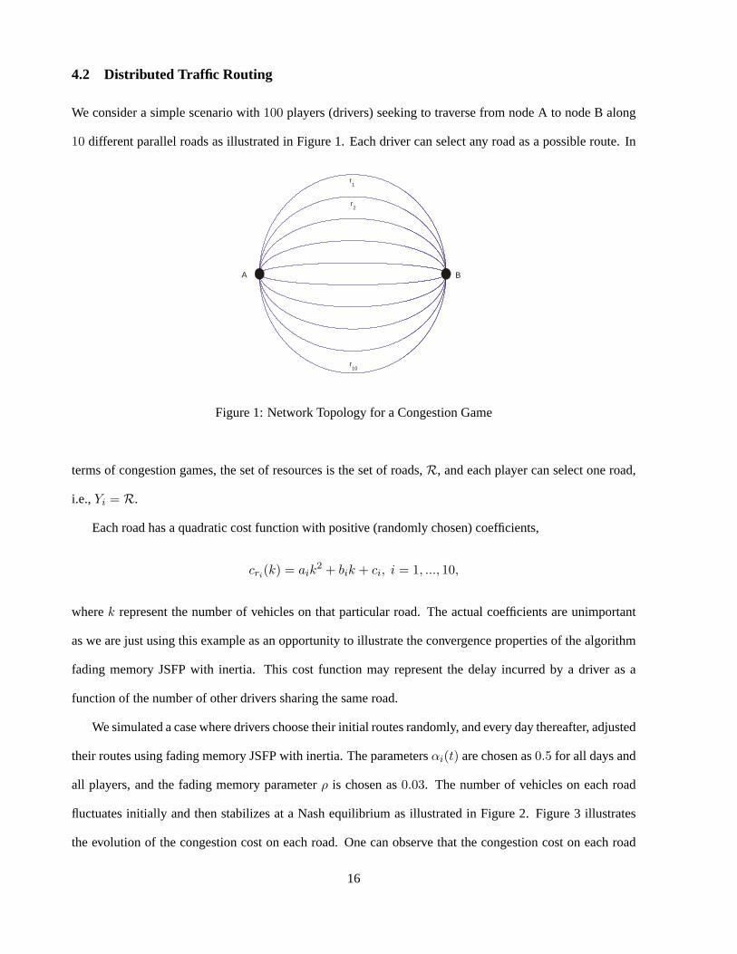
4.2 Distributed Traffic Routing

We consider a simple scenario with100 players (drivers) seeking to traverse from node A to node B along

10 different parallel roads as illustrated in Figure 1. Each driver can select any road as a possible route. In

A B

r1

r2

r10

Figure 1: Network Topology for a Congestion Game

terms of congestion games, the set of resources is the set of roads,R, and each player can select one road,

i.e.,Yi = R.

Each road has a quadratic cost function with positive (randomly chosen) coefficients,

cri(k) = aik2 + bik + ci, i = 1, ..., 10,

wherek represent the number of vehicles on that particular road. The actual coefficients are unimportant

as we are just using this example as an opportunity to illustrate the convergence properties of the algorithm

fading memory JSFP with inertia. This cost function may represent the delay incurred by a driver as a

function of the number of other drivers sharing the same road.

We simulated a case where drivers choose their initial routes randomly, and every day thereafter, adjusted

their routes using fading memory JSFP with inertia. The parametersαi(t) are chosen as0.5 for all days and

all players, and the fading memory parameterρ is chosen as0.03. The number of vehicles on each road

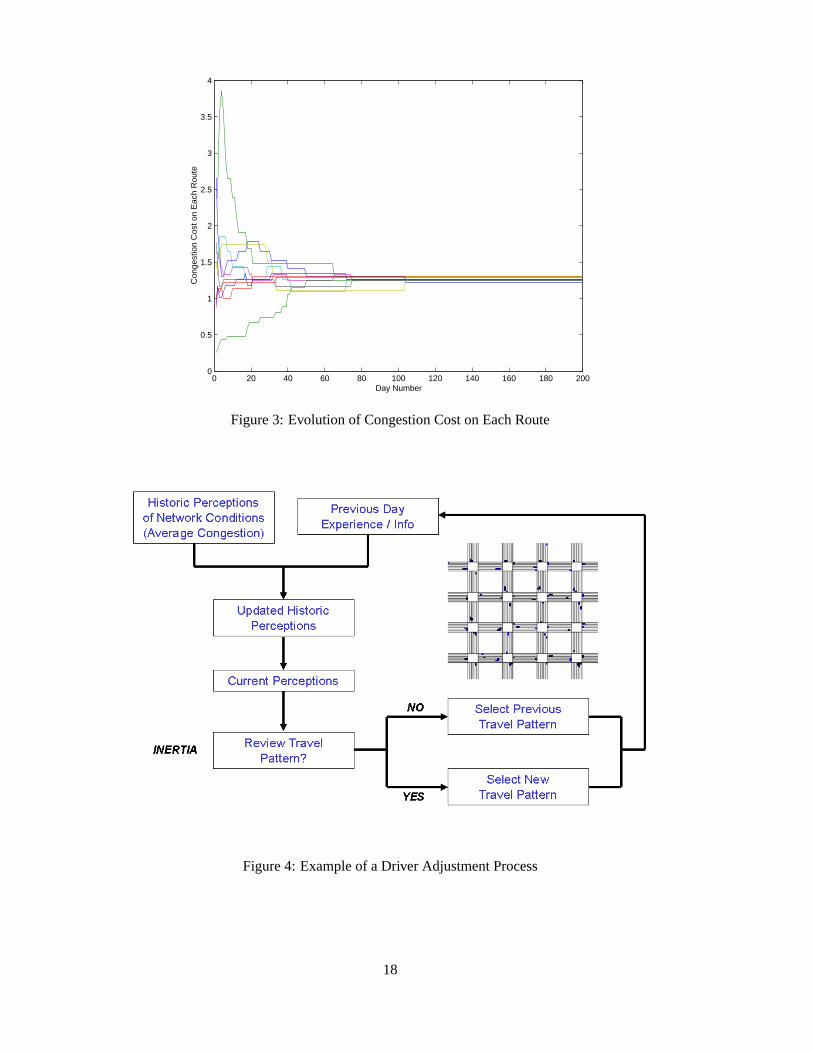
fluctuates initially and then stabilizes at a Nash equilibrium as illustrated in Figure 2. Figure 3 illustrates

the evolution of the congestion cost on each road. One can observe that the congestion cost on each road

16

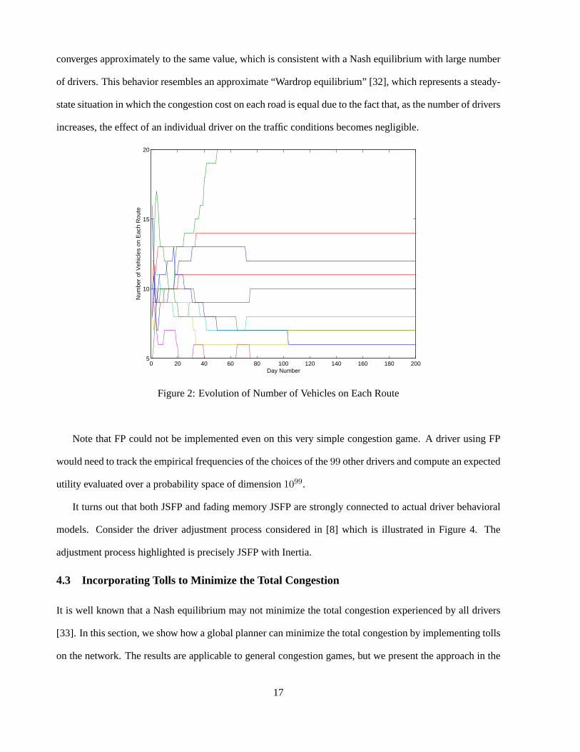
converges approximately to the same value, which is consistent with a Nash equilibrium with large number

of drivers. This behavior resembles an approximate “Wardrop equilibrium” [32], which represents a steady-

state situation in which the congestion cost on each road is equal due to the fact that, as the number of drivers

increases, the effect of an individual driver on the traffic conditions becomes negligible.

0 20 40 60 80 100 120 140 160 180 2005

10

15

20

Day Number

Num

ber

of V

ehic

les

on E

ach

Rou

te

Figure 2: Evolution of Number of Vehicles on Each Route

Note that FP could not be implemented even on this very simple congestion game. A driver using FP

would need to track the empirical frequencies of the choices of the99 other drivers and compute an expected

utility evaluated over a probability space of dimension1099.

It turns out that both JSFP and fading memory JSFP are strongly connected to actual driver behavioral

models. Consider the driver adjustment process considered in [8] which is illustrated in Figure 4. The

adjustment process highlighted is precisely JSFP with Inertia.

4.3 Incorporating Tolls to Minimize the Total Congestion

It is well known that a Nash equilibrium may not minimize the total congestion experienced by all drivers

[33]. In this section, we show how a global planner can minimize the total congestion by implementing tolls

on the network. The results are applicable to general congestion games, but we present the approach in the

17

0 20 40 60 80 100 120 140 160 180 2000

0.5

1

1.5

2

2.5

3

3.5

4

Day Number

Con

gest

ion

Cos

t on

Eac

h R

oute

Figure 3: Evolution of Congestion Cost on Each Route

Figure 4: Example of a Driver Adjustment Process

18

language of distributed traffic routing.

The total congestion experienced by all drivers on the network is

Tc(y) :=∑r∈R

σr(y)cr(σr(y)).

Define a new congestion game where each driver’s utility takes the form

Ui(y) = −∑r∈yi

(cr(σr(y)) + tr(σr(y))

),

wheretr(·) is the toll imposed on roadr which is a function of the number of users of roadr.

The following proposition outlines how to incorporate tolls so that the minimum congestion solution is

a Nash equilibrium. The approach is similar to the taxation approaches for nonatomic congestion games

proposed in [31, 34].

Proposition 4.1 Consider a congestion game of any network topology. If the imposed tolls are set as

tr(k) = (k − 1)[cr(k)− cr(k − 1)], ∀k ≥ 1,

then the total negative congestion experienced by all drivers,φc(y) := −Tc(y), is a potential function for

the congestion game with tolls.

Proof Let y1 = {y1i , y−i} andy2 = {y2

i , y−i}. We will use the shorthand notationσy1

r to represent

σr(y1). The change in utility incurred by theith driver in changing from routey2i to routey1

i is

Ui(y1)− Ui(y2) = −∑r∈y1

i

(cr(σy1

r ) + tr(σy1

r ))

+∑r∈y2

i

(cr(σy2

r ) + tr(σy2

r )),

= −∑

r∈y1i \y2

i

(cr(σy1

r ) + tr(σy1

r ))

+∑

r∈y2i \y1

i

(cr(σy2

r ) + tr(σy2

r )).

The change in the total negative congestion from the joint actiony2 to y1 is

φc(y1)− φc(y2) = −∑

r∈(y1i ∪y2

i )

(σy1

r cr(σy1

r )− σy2

r cr(σy2

r )).

Since

∑r∈(y1

i ∩y2i )

(σy1

r cr(σy1

r )− σy2

r cr(σy2

r ))

= 0,

19

the change in the total negative congestion is

φc(y1)− φc(y2) = −∑

r∈y1i \y2

i

(σy1

r cr(σy1

r )− σy2

r cr(σy2

r ))−

∑r∈y2

i \y1i

(σy1

r cr(σy1

r )− σy2

r cr(σy2

r )).

Expanding the first term, we obtain

∑r∈y1

i \y2i

(σy1

r cr(σy1

r )− σy2

r cr(σy2

r ))

=∑

r∈y1i \y2

i

(σy1

r cr(σy1

r )− (σy1

r − 1)cr(σy1

r − 1)),

=∑

r∈y1i \y2

i

(cr(σy1

r ) + tr(σy1

r )).

Therefore,

φc(y1)− φc(y2) = −∑

r∈y1i \y2

i

(cr(σy1

r ) + tr(σy1

r ))

+∑

r∈y2i \y1

i

(cr(σy2

r ) + tr(σy2

r )),

= Ui(y1)− Ui(y2).

2

By implementing the tolling scheme set forth in Proposition 4.1, we guarantee that all action profiles

that minimize the total congestion experienced on the network are equilibria of the congestion game with

tolls. However, there may be additional equilibria at which an inefficient operating condition can still occur.

The following proposition establishes the uniqueness of a strict Nash equilibrium for congestion games on

parallel network topologies such as the one considered in this example.

Proposition 4.2 Consider a congestion game with nondecreasing congestion functions where each driver

is allowed to select any one road, i.e.Yi = R for all drivers. If the congestion game has at least one strict

equilibrium, then all equilibria have the same aggregate vehicle distribution over the network. Furthermore,

all equilibria are strict.

Proof Suppose action profilesy1 andy2 are equilibria withy1 being a strict equilibrium. We will again

use the shorthand notationσy1

r to representσr(y1). Letσ(y1) := (σy1

r1 , ..., σy1

rn) andσ(y2) := (σy2

r1 , ..., σy2

rn)

be the aggregate vehicle distribution over the network for equilibriumy1 andy2. If σ(y1) 6= σ(y2), there

20

exists a roada such thatσy1

a > σy2

a and a roadb such thatσy1

b < σy2

b . Therefore, we know that

ca(σy1

a ) ≥ ca(σy2

a + 1),

cb(σy2

b ) ≥ cb(σy1

b + 1).

Sincey1 andy2 are equilibrium withy1 being strict,

ca(σy1

a ) < cri(σy1

ri+ 1), ∀ri ∈ R,

cb(σy2

b ) ≤ cri(σy2

ri+ 1), ∀ri ∈ R.

Using the above inequalities, we can show that

ca(σy1

a ) ≥ ca(σy2

a + 1) ≥ cb(σy2

b ) ≥ cb(σy1

b + 1) > ca(σy1

a ),

which gives us a contradiction. Thereforeσ(y1) = σ(y2). Sincey1 is a strict equilibrium, theny2 must be

a strict equilibrium as well. 2

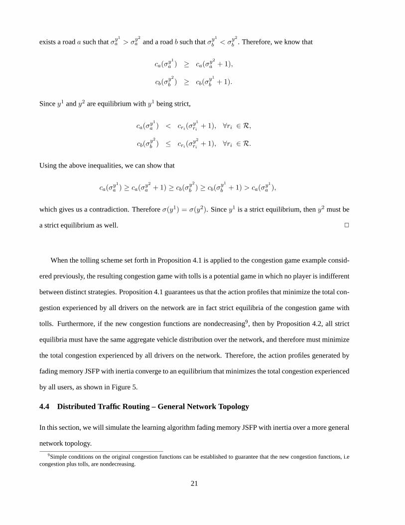
When the tolling scheme set forth in Proposition 4.1 is applied to the congestion game example consid-

ered previously, the resulting congestion game with tolls is a potential game in which no player is indifferent

between distinct strategies. Proposition 4.1 guarantees us that the action profiles that minimize the total con-

gestion experienced by all drivers on the network are in fact strict equilibria of the congestion game with

tolls. Furthermore, if the new congestion functions are nondecreasing9, then by Proposition 4.2, all strict

equilibria must have the same aggregate vehicle distribution over the network, and therefore must minimize

the total congestion experienced by all drivers on the network. Therefore, the action profiles generated by

fading memory JSFP with inertia converge to an equilibrium that minimizes the total congestion experienced

by all users, as shown in Figure 5.

4.4 Distributed Traffic Routing – General Network Topology

In this section, we will simulate the learning algorithm fading memory JSFP with inertia over a more general

network topology.

9Simple conditions on the original congestion functions can be established to guarantee that the new congestion functions, i.econgestion plus tolls, are nondecreasing.

21

0 20 40 60 80 100 120 140 160 180 20090

100

110

120

130

140

150

160

Day Number

Tot

al C

onge

stio

n E

xper

ienc

ed b

y al

l Driv

ers

Congestion Game without TollsCongestion Game With Tolls

Figure 5: Evolution of Total Congestion Experienced by All Drivers.

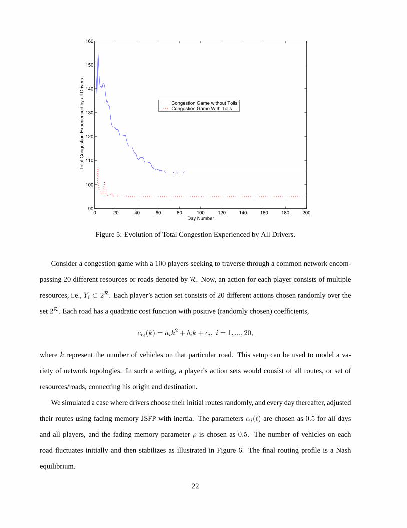
Consider a congestion game with a100 players seeking to traverse through a common network encom-

passing 20 different resources or roads denoted byR. Now, an action for each player consists of multiple

resources, i.e.,Yi ⊂ 2R. Each player’s action set consists of 20 different actions chosen randomly over the

set2R. Each road has a quadratic cost function with positive (randomly chosen) coefficients,

cri(k) = aik2 + bik + ci, i = 1, ..., 20,

wherek represent the number of vehicles on that particular road. This setup can be used to model a va-

riety of network topologies. In such a setting, a player’s action sets would consist of all routes, or set of

resources/roads, connecting his origin and destination.

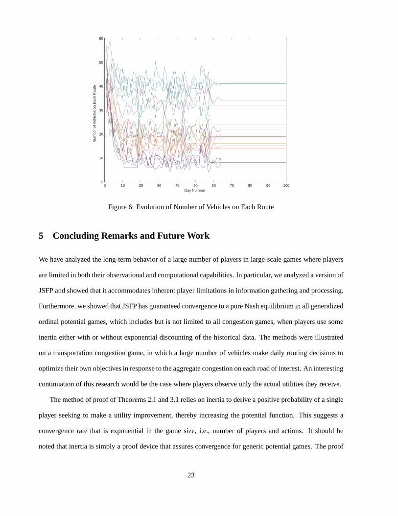
We simulated a case where drivers choose their initial routes randomly, and every day thereafter, adjusted

their routes using fading memory JSFP with inertia. The parametersαi(t) are chosen as0.5 for all days

and all players, and the fading memory parameterρ is chosen as0.5. The number of vehicles on each

road fluctuates initially and then stabilizes as illustrated in Figure 6. The final routing profile is a Nash

equilibrium.

22

0 10 20 30 40 50 60 70 80 90 1000

10

20

30

40

50

60

Day Number

Num

ber o

f Veh

icle

s on

Eac

h R

oute

Figure 6: Evolution of Number of Vehicles on Each Route

5 Concluding Remarks and Future Work

We have analyzed the long-term behavior of a large number of players in large-scale games where players

are limited in both their observational and computational capabilities. In particular, we analyzed a version of

JSFP and showed that it accommodates inherent player limitations in information gathering and processing.

Furthermore, we showed that JSFP has guaranteed convergence to a pure Nash equilibrium in all generalized

ordinal potential games, which includes but is not limited to all congestion games, when players use some

inertia either with or without exponential discounting of the historical data. The methods were illustrated

on a transportation congestion game, in which a large number of vehicles make daily routing decisions to

optimize their own objectives in response to the aggregate congestion on each road of interest. An interesting

continuation of this research would be the case where players observe only the actual utilities they receive.

The method of proof of Theorems 2.1 and 3.1 relies on inertia to derive a positive probability of a single

player seeking to make a utility improvement, thereby increasing the potential function. This suggests a

convergence rate that is exponential in the game size, i.e., number of players and actions. It should be

noted that inertia is simply a proof device that assures convergence for generic potential games. The proof

23

provides just one out of multiple paths to convergence. The simulations reflect that convergence can be

much faster. Indeed, simulations suggest that convergence is possible even in the absence of inertia but

not necessarily for all potential games. Furthermore, recent work [35] suggests that convergence rates of a

broad class of distributed learning processes can be exponential in the game size as well, and so this seems

to be a limitation in the framework of distributed learning rather than any specific learning process (as

opposed to centralized algorithms for computing an equilibrium). An important research direction involves

characterizing the convergence rates for general multi-agent learning algorithms such as JSFP.

6 Appendix

6.1 Proof of Theorem 2.1

The appendix is devoted to the proof of Theorem 2.1. It will be helpful to note the following simple obser-

vations:

1. The expression forUi(yi, z−i(t)) in equation (5) is linear inz−i(t).

2. If an action profile,y0 ∈ Y , is repeated over the interval[t, t+N − 1], i.e.,

y(t) = y(t+ 1) = ... = y(t+N − 1) = y0,

thenz(t+N) can be written as

z(t+N) =t

t+Nz(t) +

N

t+Nvy0

,

and likewisez−i(t+N) can be written as

z−i(t+N) =t

t+Nz−i(t) +

N

t+Nvy0

−i .

We begin by defining the quantitiesδi(t), Mu, mu, andγ as follows. Assume that playerPi played a

best response at least one time in the period[0, t], wheret ∈ [0,∞). Define

δi(t) := min{0 ≤ τ ≤ t : yi(t− τ) ∈ BRi(z−i(t− τ))}.

In other words,t − δi(t) is the last time in the period[0, t] at which playerPi played a best response. If

playerPi never played a best response in the period[0, t], then we adopt the conventionδi(t) = ∞. Note

24

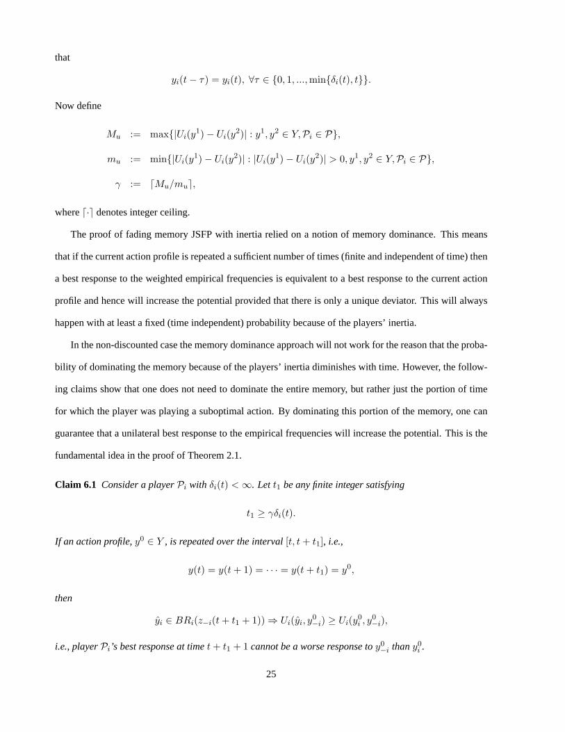
that

yi(t− τ) = yi(t), ∀τ ∈ {0, 1, ...,min{δi(t), t}}.

Now define

Mu := max{|Ui(y1)− Ui(y2)| : y1, y2 ∈ Y,Pi ∈ P},

mu := min{|Ui(y1)− Ui(y2)| : |Ui(y1)− Ui(y2)| > 0, y1, y2 ∈ Y,Pi ∈ P},

γ := dMu/mue,

whered·e denotes integer ceiling.

The proof of fading memory JSFP with inertia relied on a notion of memory dominance. This means

that if the current action profile is repeated a sufficient number of times (finite and independent of time) then

a best response to the weighted empirical frequencies is equivalent to a best response to the current action

profile and hence will increase the potential provided that there is only a unique deviator. This will always

happen with at least a fixed (time independent) probability because of the players’ inertia.

In the non-discounted case the memory dominance approach will not work for the reason that the proba-

bility of dominating the memory because of the players’ inertia diminishes with time. However, the follow-

ing claims show that one does not need to dominate the entire memory, but rather just the portion of time

for which the player was playing a suboptimal action. By dominating this portion of the memory, one can

guarantee that a unilateral best response to the empirical frequencies will increase the potential. This is the

fundamental idea in the proof of Theorem 2.1.

Claim 6.1 Consider a playerPi with δi(t) <∞. Let t1 be any finite integer satisfying

t1 ≥ γδi(t).

If an action profile,y0 ∈ Y , is repeated over the interval[t, t+ t1], i.e.,

y(t) = y(t+ 1) = · · · = y(t+ t1) = y0,

then

yi ∈ BRi(z−i(t+ t1 + 1)) ⇒ Ui(yi, y0−i) ≥ Ui(y0

i , y0−i),

i.e., playerPi’s best response at timet+ t1 + 1 cannot be a worse response toy0−i thany0

i .

25

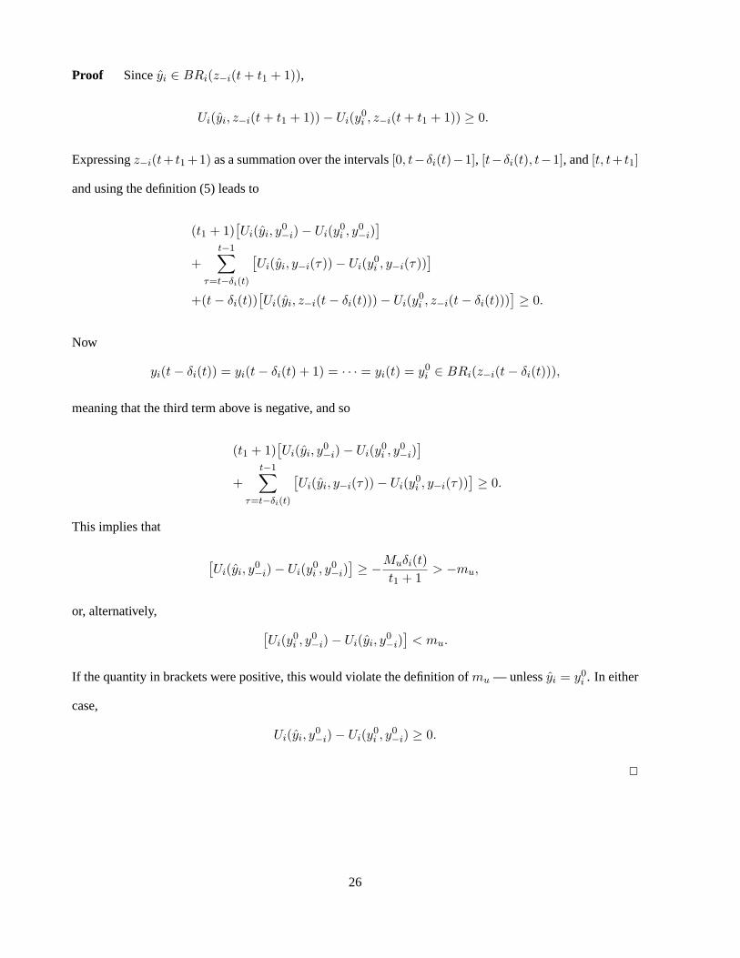
Proof Sinceyi ∈ BRi(z−i(t+ t1 + 1)),

Ui(yi, z−i(t+ t1 + 1))− Ui(y0i , z−i(t+ t1 + 1)) ≥ 0.

Expressingz−i(t+ t1 +1) as a summation over the intervals[0, t−δi(t)−1], [t−δi(t), t−1], and[t, t+ t1]

and using the definition (5) leads to

(t1 + 1)[Ui(yi, y

0−i)− Ui(y0

i , y0−i)

]+

t−1∑τ=t−δi(t)

[Ui(yi, y−i(τ))− Ui(y0

i , y−i(τ))]

+(t− δi(t))[Ui(yi, z−i(t− δi(t)))− Ui(y0

i , z−i(t− δi(t)))]≥ 0.

Now

yi(t− δi(t)) = yi(t− δi(t) + 1) = · · · = yi(t) = y0i ∈ BRi(z−i(t− δi(t))),

meaning that the third term above is negative, and so

(t1 + 1)[Ui(yi, y

0−i)− Ui(y0

i , y0−i)

]+

t−1∑τ=t−δi(t)

[Ui(yi, y−i(τ))− Ui(y0

i , y−i(τ))]≥ 0.

This implies that

[Ui(yi, y

0−i)− Ui(y0

i , y0−i)

]≥ −Muδi(t)

t1 + 1> −mu,

or, alternatively, [Ui(y0

i , y0−i)− Ui(yi, y

0−i)

]< mu.

If the quantity in brackets were positive, this would violate the definition ofmu — unlessyi = y0i . In either

case,

Ui(yi, y0−i)− Ui(y0

i , y0−i) ≥ 0.

2

26

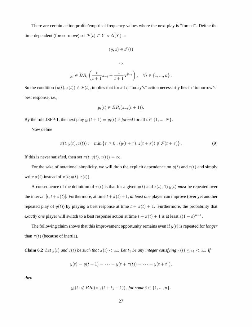
There are certain action profile/empirical frequency values where the next play is “forced”. Define the

time-dependent (forced-move) setF(t) ⊂ Y ×∆(Y ) as

(y, z) ∈ F(t)

⇔

yi ∈ BRi

(t

t+ 1z−i +

1t+ 1

vy−i

), ∀i ∈ {1, ..., n} .

So the condition(y(t), z(t)) ∈ F(t), implies that for alli, “today’s” action necessarily lies in “tomorrow’s”

best response, i.e.,

yi(t) ∈ BRi(z−i(t+ 1)).

By the rule JSFP-1, the next playyi(t+ 1) = yi(t) is forcedfor all i ∈ {1, ..., N}.

Now define

π(t; y(t), z(t)) := min {τ ≥ 0 : (y(t+ τ), z(t+ τ)) 6∈ F(t+ τ)} . (9)

If this is never satisfied, then setπ(t; y(t), z(t)) = ∞.

For the sake of notational simplicity, we will drop the explicit dependence ony(t) andz(t) and simply

write π(t) instead ofπ(t; y(t), z(t)).

A consequence of the definition ofπ(t) is that for a giveny(t) andz(t), 1) y(t) mustbe repeated over

the interval[t, t+π(t)]. Furthermore, at timet+π(t)+1, at least oneplayer can improve (over yet another

repeated play ofy(t)) by playing a best response at timet + π(t) + 1. Furthermore, the probability that

exactly oneplayer will switch to a best response action at timet+ π(t) + 1 is at leastε(1− ε)n−1.

The following claim shows that this improvement opportunity remains even ify(t) is repeated forlonger

thanπ(t) (because of inertia).

Claim 6.2 Lety(t) andz(t) be such thatπ(t) <∞. Let t1 be any integer satisfyingπ(t) ≤ t1 <∞. If

y(t) = y(t+ 1) = · · · = y(t+ π(t)) = · · · = y(t+ t1),

then

yi(t) 6∈ BRi(z−i(t+ t1 + 1)), for somei ∈ {1, ..., n}.

27

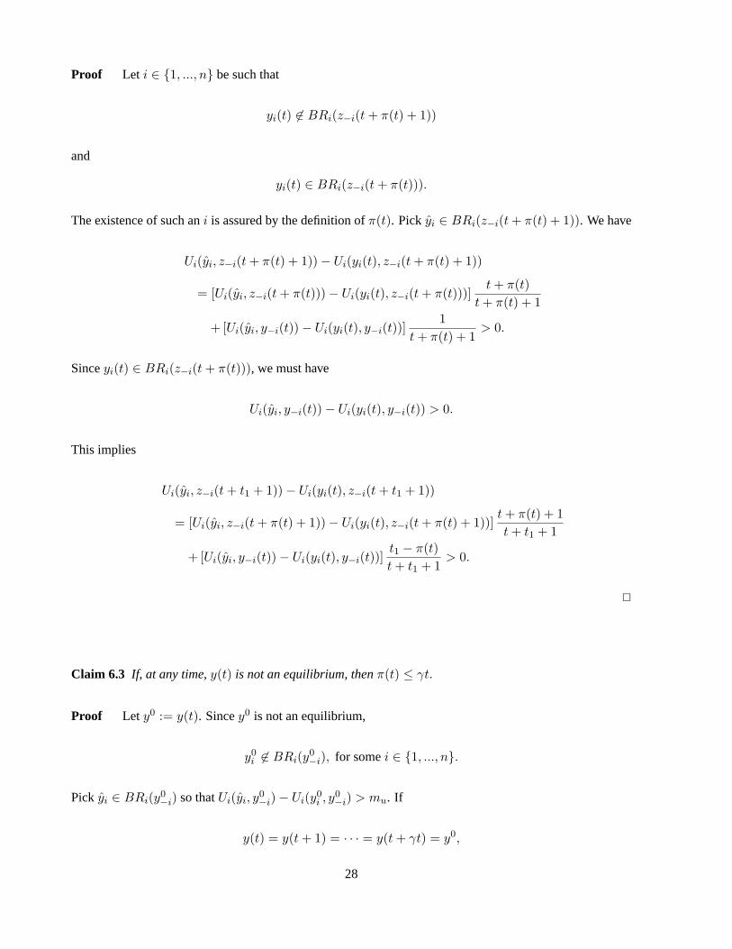
Proof Let i ∈ {1, ..., n} be such that

yi(t) 6∈ BRi(z−i(t+ π(t) + 1))

and

yi(t) ∈ BRi(z−i(t+ π(t))).

The existence of such ani is assured by the definition ofπ(t). Pick yi ∈ BRi(z−i(t+ π(t) + 1)). We have

Ui(yi, z−i(t+ π(t) + 1))− Ui(yi(t), z−i(t+ π(t) + 1))

= [Ui(yi, z−i(t+ π(t)))− Ui(yi(t), z−i(t+ π(t)))]t+ π(t)

t+ π(t) + 1

+ [Ui(yi, y−i(t))− Ui(yi(t), y−i(t))]1

t+ π(t) + 1> 0.

Sinceyi(t) ∈ BRi(z−i(t+ π(t))), we must have

Ui(yi, y−i(t))− Ui(yi(t), y−i(t)) > 0.

This implies

Ui(yi, z−i(t+ t1 + 1))− Ui(yi(t), z−i(t+ t1 + 1))

= [Ui(yi, z−i(t+ π(t) + 1))− Ui(yi(t), z−i(t+ π(t) + 1))]t+ π(t) + 1t+ t1 + 1

+ [Ui(yi, y−i(t))− Ui(yi(t), y−i(t))]t1 − π(t)t+ t1 + 1

> 0.

2

Claim 6.3 If, at any time,y(t) is not an equilibrium, thenπ(t) ≤ γt.

Proof Let y0 := y(t). Sincey0 is not an equilibrium,

y0i 6∈ BRi(y0

−i), for somei ∈ {1, ..., n}.

Pick yi ∈ BRi(y0−i) so thatUi(yi, y

0−i)− Ui(y0

i , y0−i) > mu. If

y(t) = y(t+ 1) = · · · = y(t+ γt) = y0,

28

then

Ui(yi, z−i(t+ γt+ 1))− Ui(y0i , z−i(t+ γt+ 1))

=t[Ui(yi, z−i(t))− Ui(y0

i , z−i(t))] + (γt+ 1)[Ui(yi, y0−i)− Ui(y0

i , y0−i)]

t+ γt+ 1

≥ −tMu + (γt+ 1)mu

t+ γt+ 1

> 0.

2

Claim 6.4 Consider a finite generalized ordinal potential game with a potential functionφ(·) with player

utilities satisfying Assumption 2.2. For any timet ≥ 0, suppose that

1. y(t) is not an equilibrium; and

2. max1≤i≤n δi(t) ≤ δ for someδ ≤ t.

Define

ψ(t) := 1 + max{π(t), γδ

}.

Thenψ(t) ≤ 1 + γt and

Pr [φ(y(t+ ψ(t))) > φ(y(t)) | y(t), z(t)] ≥ ε(1− ε)n(1+γδ)−1,

and

max1≤i≤n

δi(t+ ψ(t)) ≤ 1 + (1 + γ)δ.

Proof Sincey(t) is not an equilibrium, Claim 6.3 implies thatπ(t) ≤ γt, which in turn implies the above

upper bound onψ(t).

First consider the case whereπ(t) ≥ γδ, i.e.,ψ(t) = 1 + π(t). According to the definition ofπ(t) in

equation (9),y(t) mustbe repeated as a best response in the period[t, t+ π(t)]. Furthermore, we must have

max1≤i≤n

δi(t+ ψ(t)) ≤ 1

29

andyi(t) 6∈ BRi(z−i(t+ ψ(t))) for at least one playerPi. The probability that exactly one such playerPi

will switch to a choice different thanyi(t) at timet + ψ(t) is at leastε(1 − ε)n−1. But, by Claim 6.1 and

no-indifference Assumption 2.2, such an event would cause

Ui(y(t+ π(t) + 1)) > Ui(y(t)) ⇒ φ(y(t+ π(t) + 1)) > φ(y(t)).

Now consider the case whereπ(t) < γδ, i.e.,ψ(t) = 1 + γδ. In this case,

max1≤i≤n

δi(t+ ψ(t)) ≤ 1 + γδ + δ.

Moreover, the event

y(t) = · · · = y(t+ γδ)

will occur with probability at least10 (1− ε)nγδ. Conditioned on this event, Claim 6.2 provides that exactly

one playerPi will switch to a choice different thanyi(t) at timet+ψ(t) with probability at leastε(1−ε)n−1.

By Claim 6.1 and no-indifference Assumption 6, this would cause

Ui(y(t+ ψ(t))) > Ui(y(t)) ⇒ φ(y(t+ ψ(t))) > φ(y(t)).

2

Proof of Theorem 2.1

It suffices to show that there exists a non-zero probability,ε∗ > 0, such that the following statement holds.

For anyt ≥ 0, y(t) ∈ Y , andz(t) ∈ ∆(Y ), there exists a finite timet∗ ≥ t such that, for some equilibrium

y∗,

Pr [y(τ) = y∗,∀τ ≥ t∗ | y(t), {z−i(t)}ni=1] ≥ ε∗. (10)

In other words, the probability of convergence to an equilibrium by timet∗ is at leastε∗. Sinceε∗ does not

depend ont, y(t), or z(t), this will imply that the action profile converges to an equilibrium almost surely.

We will construct a series of events that can occur with positive probability to establish the bound in

equation (10).

10In fact, a tighter bound can be derived by exploiting the forced moves for a duration ofπ(t).

30

Let t0 = t + 1. All players will play a best response at timet0 with probability at leastεn. Therefore,

we have

Pr[

max1≤i≤n

δi(t0) = 0 | y(t), {z−i(t)}ni=1

]≥ εn. (11)

Assume thaty(t0) is not an equilibrium. Otherwise, according to Proposition 2.2,y(τ) = y(t0) for all

τ ≥ t0.

From Claim 6.4, definet1 andδ1 as

δ1 := 1 + (1 + γ)δ0,

t1 := t0 + 1 + max{π(t0), γδ0},

≤ t0 + 1 + γt0 = 1 + (1 + γ)t0,

whereδ0 := 0. By Claim 6.4,

Pr [φ(y(t1)) > φ(y(t0)) | y(t0), {z−i(t0)}ni=1] ≥ ε(1− ε)n(1+γδ0)−1

and

max1≤i≤n

δi(t1) ≤ δ1.

Similarly, for k > 0 we can recursively define

δk := 1 + (1 + γ)δk−1,

= (1 + γ)kδ0 +k−1∑j=0

(1 + γ)j ,

=k−1∑j=0

(1 + γ)j

and

tk := tk−1 + 1 + max{π(tk−1), γδk−1},

≤ 1 + (1 + γ)tk−1,

≤ (1 + γ)kt0 +k−1∑j=0

(1 + γ)j

where

Pr [φ(y(tk)) > φ(y(tk−1)) | y(tk−1), {z−i(tk−1)}ni=1] ≥ ε(1− ε)n(1+γδk−1)−1

31

and

max1≤i≤n

δi(tk) ≤ δk,

as long asy(tk−1) is not an equilibrium.

Therefore, one can construct a sequence of profilesy(t0), y(t1), ..., y(tk) with the property thatφ(y(t0)) <

φ(y(t1)) < ... < φ(y(tk)). Since in a finite generalized ordinal potential game,φ(y(tk)) cannot increase

indefinitely ask increases, we must have

Pr [y(tk) is an equilibrium for sometk ∈ [t,∞) | y(t), {z−i(t)}ni=1] ≥ εn

|Y |−1∏k=0

ε(1− ε)n(1+γδk)−1,

whereεn comes from (11). Finally, from Claim 6.1 and Assumption 2.2, the above inequality together with

Pr [y(tk) = · · · = y(tk + γδk) | y(tk), {z−i(tk)}ni=1] ≥ (1− ε)nγδk ≥ (1− ε)nγδ|Y |

implies that for some equilibrium,y∗,

Pr [y(τ) = y∗, ∀τ ≥ t∗ | y(t), {z−i(t)}ni=1] ≥ ε∗,

where

t∗ = t|Y | + γδ|Y | + 1 = (1 + γ)|Y |t0 +|Y |∑j=0

(1 + γ)j ,

ε∗ =(εn

|Y |−1∏k=0

ε(1− ε)n(1+γδk)−1

)((1− ε)nγδ|Y |

).

Sinceε∗ does not depend ont this concludes the proof. 2

References

[1] J. R. Marden, G. Arslan, and J. S. Shamma, “Joint strategy fictitious play with inertia for potentialgames,” inProceedings of the 44th IEEE Conference on Decision and Control, December 2005, pp.6692–6697.

[2] D. Fudenberg and D. K. Levine,The Theory of Learning in Games. Cambridge, MA: MIT Press,1998.

[3] H. P. Young,Strategic Learning And Its Limits. Oxford University Press, 2005.

32

[4] D. Fudenberg and D. Kreps, “Learning mixed equilibria,”Games and Economic Behavior, vol. 5,no. 3, pp. 320–367, 1993.

[5] D. Monderer and A. Sela, “Fictitious play and no-cycling conditions,” Tech. Rep., 1997. [Online].Available: http://www.sfb504.uni-mannheim.de/publications/dp97-12.pdf

[6] R. W. Rosenthal, “A class of games possessing pure-strategy nash equilibria,”International Journal ofGame Theory, vol. 2, pp. 65–67, 1973.

[7] M. Ben-Akiva and S. Lerman,Discrete-Choice Analysis: Theory and Application to Travel Demand.Cambridge, MA: MIT Press, 1985.

[8] M. Ben-Akiva, A. de Palma, and I. Kaysi, “Dynamic network models and driver information systems,”Transportation Research A, vol. 25A, pp. 251–266, 1991.

[9] H. P. Young,Individual Strategy and Social Structure. Princeton, NJ: Princeton University Press,1998.

[10] J. Hofbauer and K. Sigmund,Evolutionary Games and Population Dynamics. Cambridge UniversityPress, 1998.

[11] J. W. Weibull,Evolutionary Game Theory. Cambridge, MA: MIT Press, 1995.

[12] S. Hart, “Adaptive heuristics,”Econometrica, vol. 73, no. 5, pp. 1401–1430, 2005.

[13] S. Hart and A. Mas-Colell, “Uncoupled dynamics do not lead to Nash equilibrium,”American Eco-nomic Review, vol. 93, no. 5, pp. 1830–1836, 2003.

[14] J. S. Shamma and G. Arslan, “Dynamic fictitious play, dynamic gradient play, and distributed con-vergence to Nash equilibria,”IEEE Transactions on Automatic Control, vol. 50, no. 3, pp. 312–327,2005.

[15] G. Arslan and J. S. Shamma, “Distributed convergence to Nash equilibria with local utility measure-ments,” inProceedings of the 43rd IEEE Conference on Decision and Control, 2004, pp. 1538–1543.

[16] T. Lambert, M. Epelman, and R. Smith, “A fictitious play approach to large-scale optimization,”Op-erations Research, vol. 53, no. 3, pp. 477–489, 2005.

[17] H. P. Young, “The evolution of conventions,”Econometrica, vol. 61, no. 1, pp. 57–84, 1993.

[18] S. Hart and A. Mas-Colell, “A simple adaptive procedure leading to correlated equilibrium,”Econo-metrica, vol. 68, no. 5, pp. 1127–1150, 2000.

[19] ——, “Regret based continuous-time dynamics,”Games and Economic Behavior, vol. 45, pp. 375–394, 2003.

[20] R. S. Sutton and A. G. Barto,Reinforcement Learning: An Introduction. MA: MIT Press, 1998.

[21] D. P. Bertsekas and J. N. Tsitsiklis,Neuro-Dynamic Programming. Belmont, MA: Athena Scientific,1996.

[22] D. Leslie and E. Collins, “Convergent multiple-timescales reinforcement learning algorithms in normalform games,”Annals of Applied Probability, vol. 13, pp. 1231–1251, 2003.

33

[23] ——, “Individual Q-learning in normal form games,”SIAM Journal on Control and Optimization,vol. 44, pp. 495–514, 2005.

[24] ——, “Generalised weakened fictitious play,”Games and Economic Behavior, vol. 56, pp. 285–298,2005.

[25] S. Huck and R. Sarin, “Players with limited memory,”Contributions to Theoretical Economics, vol. 4,no. 1, 2004.

[26] S. Fischer and B. Vocking, “The evolution of selfish routing,” inProceedings of the 12th EuropeanSymposium on Algorithms (ESA ’04), 2004, pp. 323–334.

[27] S. Fischer and B. Voecking, “Adaptive routing with stale information,” inProceedings of the 24thAnnual ACM Symposium on Principles of Distributed Computing, 2005, pp. 276–283.

[28] S. Fischer, H. Raecke, and B. Voecking, “Fast convergence to Wardrop equilibria by adaptive samplingmethods,” inProceedings of the 38th Annual ACM Symposium on Theory of Computing, 2006, pp.653–662.

[29] A. Blum, E. Even-Dar, and K. Ligett, “Routing without regret: On convergence to Nash equilibria ofregret-minimizing algorithms in routing games,” inProceedings of the 25th Annual ACM Symposiumon Principles of Distributed Computing, 2006, pp. 45–52.

[30] D. Monderer and L. S. Shapley, “Potential games,”Games and Economic Behavior, vol. 14, pp. 124–143, 1996.

[31] I. Milchtaich, “Social optimality and cooperation in nonatomic congestion games,”Journal of Eco-nomic Theory, vol. 114, no. 1, pp. 56–87, 2004.

[32] J. G. Wardrop, “Some theoretical aspects of road traffic research,” inProceedings of the Institute ofCivil Engineers, vol. I, pt. II, London, Dec. 1952, pp. 325–378.

[33] T. Roughgarden, “The price of anarchy is independent of the network topology,”Journal of Computerand System Sciences, vol. 67, no. 2, pp. 341–364, 2003.

[34] W. Sandholm, “Evolutionary implementation and congestion pricing,”Review of Economic Studies,vol. 69, no. 3, pp. 667–689, 2002.

[35] S. Hart and Y. Mansour, “The communication complexity of uncoupled nash equilibrium procedures,”The Hebrew University of Jerusalem, Center for Rationality, Tech. Rep. DP-419, April 2006.

34