HAL Id: hal-01514402https://hal.inria.fr/hal-01514402

Submitted on 26 Apr 2017

HAL is a multi-disciplinary open accessarchive for the deposit and dissemination of sci-entific research documents, whether they are pub-lished or not. The documents may come fromteaching and research institutions in France orabroad, or from public or private research centers.

L’archive ouverte pluridisciplinaire HAL, estdestinée au dépôt et à la diffusion de documentsscientifiques de niveau recherche, publiés ou non,émanant des établissements d’enseignement et derecherche français ou étrangers, des laboratoirespublics ou privés.

Joint Spatial and Temporal Classification of MobileTraffic Demands

Angelo Furno, Marco Fiore, Razvan Stanica

To cite this version:Angelo Furno, Marco Fiore, Razvan Stanica. Joint Spatial and Temporal Classification of MobileTraffic Demands. INFOCOM 2017 – 36th Annual IEEE International Conference on Computer Com-munications, May 2017, Atlanta, United States. pp. 1-9. <hal-01514402>

Joint Spatial and Temporal Classificationof Mobile Traffic Demands

Angelo Furno∗†, Marco Fiore‡, Razvan Stanica∗∗ Universite de Lyon, INRIA, INSA-Lyon, CITI-INRIA, F-69621 Villeurbanne, France – name.surname@inria.fr

† Universite de Lyon, IFSTTAR, ENTPE, F-69675 Lyon, France – angelo.furno@ifsttar.fr‡ CNR – IEIIT, Corso Duca degli Abruzzi 24, 10129 Torino, Italy – marco.fiore@ieiit.cnr.it

Abstract—Mobile traffic data collected by network operators isa rich source of information about human habits, and its analysisprovides insights relevant to many fields, including urbanism,transportation, sociology and networking. In this paper, wepresent an original approach to infer both spatial and temporalstructures hidden in the mobile demand, via a first-time tailoringof Exploratory Factor Analysis (EFA) techniques to the context ofmobile traffic datasets. Casting our approach to the time or spacedimensions of such datasets allows solving different problems inmobile traffic analysis, i.e., network activity profiling and landuse detection, respectively. Tests with real-world mobile trafficdatasets show that, in both its variants above, the proposedapproach (i) yields results whose quality matches or exceedsthat of state-of-the-art solutions, and (ii) provides additional jointspatiotemporal knowledge that is critical to result interpretation.

I. INTRODUCTION

The surge in mobile data traffic –estimated globally at 3.7exabytes in 2015, with an overall 4,000-fold growth over thepast ten years [1]– has fostered a widening interest in betterunderstanding the dynamics of the mobile demand. Knowledgemining of real-world datasets has revealed important featuresthat characterize mobile traffic: examples include a strong tem-poral periodicity [2] and geographic locality [3] that enable ef-fective prediction of the demand; the appearance of significantfluctuations induced by social events [4] with the consequentneed for dedicated resource management policies; or, a neatheterogeneity of the capacity consumed by subscribers [5] thatis however captured by a limited number of typical profiles [6],which enables the informed tuning of traffic plans.

Analyses of mobile traffic demand in the literature can bedivided into two broad categories [7]: (i) works that take a userperspective, and study the behavior of individual subscribersin terms of their mobility, the traffic they generate, andthe mobile services they consume; (ii) works that take anoperator perspective, and investigate properties of the demandaggregated over all users present in a given area, typically acell sector or the coverage region of a base station.

Our work falls in the second category. Specifically, wefocus on the problem of classification, i.e., finding hiddenregular structures in the aggregate traffic generated by mobileusers. As set forth in Sec. II, previous works have proposedsolutions to detect either temporal or spatial structures in thedata, but little attention has been paid to the more challengingconcurrent inspection of both space and time dimensions.

This paper fills the gap above, by presenting an originalmethodology for the joint spatiotemporal classification of theaggregate demand supplied by a mobile network operator.The proposed methodology stems from Exploratory Factor

Analysis (EFA), a well established instrument in psychologyresearch. As detailed in Sec. III, EFA aims at identifying, ina fully automated way, latent factors that cause the dynamicsobserved in the data. When tailored to the specific use case ofmobile traffic classification, as discussed in Sec. IV, EFA offersthe possibility of exploring the space and time dimensions ofthe data at once. This yields two significant advantages.

First, the same methodology can be cast to recognize factorsthat are temporal or spatial in nature, solving the following twoproblems in mobile traffic analysis.• Network activity profiling aims at detecting temporal struc-tures in the network-wide communication activity, and allowsclassifying together time periods that show a similar, stablespatial distribution of the mobile traffic demand. Networkactivity profiles are expected to find applications in cognitivenetworking [8], where they can drive the establishment, mod-ification, release and relocation of resources, in concert withthe temporal variations in the mobile demand [9].• Land use detection is the identification of spatial structuresin the mobile traffic data, through the decomposition of ageographical area into zones where the mobile traffic dynamicsover time are homogeneous. When considering metropolitan-scale regions, these zones correspond to land uses – i.e.,the combination of urban infrastructures and predominantundertakings of people at those locations. This has applicationsin geoinformatics, as an effective way to automatically labelthe urban tissue, at lower cost and with higher accuracythan traditional survey methods [10]. It is also relevant tocognitive networking, since the discovery of city regions withanalogous demand evolution may ease the dynamic allocationof spectrum at individual base stations, helping mitigating highfluctuations of resource needs in small network areas [9].

Second, our proposed methodology allows immediate ex-trapolation of the structures hidden in the secondary dimen-sion of both problems above. In other words, it provides,at no additional cost, knowledge of the spatial patterns thatcharacterize each network activity profile, and of the precisetemporal dynamics that distinguish each land use. This playsan important role in the interpretation of classification results.

We demonstrate these advantages by performing a spa-tiotemporal classification of real-world mobile traffic datarecorded by national operators in two major European cities,in Sec. V. When compared with current state-of-the-art tech-niques dedicated to the two data analysis problems above,our solution easily matches them in terms of quality of theclassification; in addition, it simplifies the interpretation ofclasses through a combined spatiotemporal view of the same.

II. RELATED WORK

The study of traffic data collected by mobile operators hasfound applications across research domains such as urbanism,transportation, sociology, epidemiology, and telecommunica-tion networking [7]. Related to our problem are classificationsof the temporal and spatial distributions of the mobile demand.

Fine-grained temporal classifications have mainly focusedon outlying situations [11]. Specifically, both planned [12]and unplanned [13] events were found to induce significantvariations in the typical temporal structure of the mobiletraffic demand. A more complete approach to network activityprofiling has been recently presented in [14]: it is based ona dedicated, fine-tuned clustering of snapshots of the mobiletraffic demand at different time periods. We will compare theresults of our proposed solution to those obtained with thisframework in the performance evaluation in Sec. V.

As far as high-detail spatial structures in the mobile trafficare concerned, a number of works have revealed the cor-relations between the geographic diversity of mobile trafficand the urban landscape [15], [16], and employed them forautomated land use detection [10], [17], [18]. All previousland use detection algorithms represent the mobile demandin different geographical zones as time series, process themthough compression, filtering and normalization, and finallyclassify them via clustering. Among the proposed solutions,that in [18] has been shown to provide the most accurateresults, and we will this consider it as our benchmark in Sec. V.

It is important to note that all previous works explored thetemporal and spatial structures of the mobile traffic separately,and we still lack a comprehensive methodology that canaddress the two dimensions at once. In this paper, we borrowfrom EFA techniques to achieve such a goal. The roots of fac-tor analysis date back to the work of Spearman, over a centuryago [19]. Following those early studies, EFA has emerged asone of the dominant classes of factor analysis, and has beenwidely employed in statistical psychology research [20]. Tothe best of our knowledge, this is the first time factor analysisis leveraged for the study of mobile traffic data and, moregenerally, in the field of wireless networking.

III. EXPLORATORY FACTOR ANALYSIS

Here, we provide an introduction to EFA fundamentals. Westart with some terminology used in the remainder of the paper.• Variables are the set of phenomena of interest, relatedto some population of individuals. E.g., subjects taught toprimary school students.• Samples represent the set of monitored individuals from thegiven population, for which all phenomena of interest can bemeasured. E.g., students from a same class.• Observations are the realizations of all variables for eachsample. E.g., the grades of examination tests in all subjectobtained by each student.• Common factors are complex interrelationship among theobserved phenomena that the analyst can reasonably assumeto exist. In practical cases, these latent features cannot bedirectly observed in the data, due to the very large numberof variables. Then, the goal of EFA is the recognition ofsuch factors1, which are supposed to be small in number

1We will use common factor and factor interchangeably in the following.

with respect to the variables, and thus allow for an easierinterpretation of the phenomena. E.g., in our example, EFAmay aim at inferring factors such as verbal and mathematicalintelligence, whose combination could explain the averagestudent’s aptitude towards each subject.• Factor loadings are numerical relationships that describehow much each common factor explains each variable. Moreprecisely, the squared loading is the percent of variance in avariable explained by a common factor. Loadings close to the1 or -1 extremes indicate that the factor strongly affects thevariable, with a positive or negative correlation, respectively;instead, loadings close to zero indicate that the factor has aweak effect on the variable. As such, loadings are the maininstrument to label the factors returned by EFA. E.g., a factorthat has high loadings solely in algebra and geometry canreveal the existence of a common mathematical intelligencethat explains the performance of the majority of students inmathematics-related disciplines.• Factor scores are values that relate samples to commonfactors. For a given sample and factor pair, a high (low) scoreindicates that the sample has a ranking on the factor that ismuch above (below) the average. Interestingly, scores allowinspecting samples in the light of factors, and thus complementloadings when it comes to result interpretation. E.g., scoresindicate if the good (poor) performance in scientific disciplinesof any subset of students is especially well explained by theirstrong (weak) mathematical intelligence.• Unique factors model situations where the data transcendcommon factors, by explaining the unique variance associatedto each variable. Unique factors are thus useful to pinpoint out-lying behaviors in the data. E.g., unique factors can account fora rare talent of one student towards a specific discipline. Due toits peculiarity, such a talent is not captured by any intelligencetowards subjects that is commonly found in schoolchildren.

A. Fundamental model

Given a set of observed variables of interest, factor analysisis formally defined as “a model of hypothetical componentvariables that explain the linear2 relationships existing be-tween observed variables” [21]. Such a hypothetical set ofcomponent variables can be derived mathematically from theobserved variables, as follows.

Let X be a N × 1 vector of observed variables, distributedwith expectation E(X) = 0 and covariance Σ = Cov(X). Letalso F be a K × 1 vector of unknown normalized commonfactors, having mean E(F) = 0, covariance Φ = Cov(F) andorder K < N . Next, let Λ be an unknown N ×K matrix ofcommon factor pattern coefficients (i.e., factor loadings). Letalso U be a N × 1 vector of independently distributed errorterms (i.e., unique factors), with mean E(U) = 0 and finitecovariance Ψ = Cov(U). Since each unique factors is specificto one variable, the error terms are independent, and Ψ is adiagonal matrix. Finally, we want common factors and uniquefactors to be uncorrelated, i.e., Cov(F,U) = 0. Hence,

X = ΛF + U (1)

2The linearity of relationships among variables in the specific context ofmobile traffic will be discussed in Sec. IV-B.

is the fundamental equation of factor analysis, stating thatthe observed variables in X are weighted combinations of thecommon factors in F and the unique factors in U. From (1),the covariance of the observed variables X can be written as

Σ = Cov(X) = Cov(ΛF + U) =

ΛCov(F)Λᵀ + Cov(U) =

ΛΦΛᵀ + Ψ,

(2)

which represents the fundamental theorem of factor analysis.In the case of EFA, no hypotheses concerning the factorsare made, and it is thus generally assumed all factors to beorthogonal, i.e., mutually uncorrelated and with unit variances.Thus, Φ can be replaced by the identity matrix in (2), and

Σ = ΛΛᵀ + Ψ, (3)

whose i-th diagonal element can be written as

σii = Var(xi) =k∑

j=1

λ2ij + ψii = hi + ψii. (4)

From (4), the variance of each observed variable, σii,consists of two parts: the communality hi, i.e., the portion ofthe variance shared with the other variables via the commonfactors, and the unique variance ψii, i.e., the share specific toeach variable, via the associated unique factor.

B. Factor extraction

Maximum Likelihood Estimation (MLE) allows inferring theunknown variables Λ and Ψ in (3) in a way that is efficientand robust [21]. MLE assumes X in (1) to have a multivariatenormal distribution3 with mean X = 1

M

∑Ma=1 Xa and covari-

ance S = 1M−1 (

∑Ma=1 XaX

ᵀa −MXXᵀ) computed from the

M observations. MLE maximizes the likelihood function

lnL = −1

2(M − 1)[ln |Σ|+ Tr(SΣ−1)], (5)

with Tr indicating the matrix trace operator. The Σ matrixmaximizing (5) also minimizes the following fit function [22]

FK(Σ) = ln |Σ|+ Tr(SΣ−1)− ln |S| −N, (6)

where K refers to the number of common factors considered.Using (3) in (6), the expression FK(Σ) = FK(Λ,Ψ) canbe used to compute the maximum likelihood estimates of theunknowns Λ and Ψ. We outline the main steps below, whilefull details are found in [21].

Firstly, FK is minimized with respect to Λ, where theminimizer Λ is computed by imposing ∂FK

∂Λ = 0. Denotingas = the identity matrix, the above condition leads to

Λ = Ψ1/2ΩK [γi − 1]1/2K , (7)

3MLE yields good estimations even when the actual distribution of X is notmultivariate Gaussian [21]. We ran tests with alternative methods like Minresand Principal Axis that do not rely on this assumption, and they providedresults (omitted due to space limitations) consistent with those in Sec. V.

where the diagonal matrix [γi − 1]K contains the K largesteigenvalues of Ψ−1/2SΨ−1/2, and ΩK contains the corre-sponding eigenvectors. Replacing (6) in (7) one can derivethe expression of the conditional minimum for a given Ψ, as

fK(Ψ) = −N∑

j=K+1

ln γj +N∑

j=K+1

γj − (N −K), (8)

where γj , with j = K+1, . . . , N , are the residual eigenvaluesof the matrix Ψ−1/2SΨ−1/2.

Secondly, the function fK is minimized with respect to Ψ,by imposing ∂fK

∂Ψ = 0, which leads to the expression

Diag(Ψ−1(ΛΛᵀ

+ Ψ− S)Ψ−1) = 0. (9)

At this point, the maximum likelihood estimates of Λ and Ψcan be computed by means of an iterative procedure basedon the Fletcher-Powell method and applied to the function fKand its partial derivatives in (8) and (9), respectively.

C. EFA and Principal Component Analysis

The structure of the fundamental equation in (1) hints atthe fact that factor analysis is a close relative of PrincipalComponent Analysis (PCA), a popular tool for multivariateanalysis. Therefore, a legitimate question is why EFA is morerelevant than PCA to the problem we are trying to solve, i.e,the classification of mobile traffic demands.

To answer this question, we recall that PCA aims at findingorthogonal linear combinations of the variables that maximizethe total variance in the data. In other words, PCA looks forthe major sources of variation in data, or, equivalently, for thelowest number of components that explain the available obser-vations. Such an objective lends itself to data dimensionalityreduction, which is in fact the natural application of PCA.

EFA fundamentally differs from PCA in that it distinguishesbetween shared and unique variances in the data, modelledby common and unique factors, respectively. This isolatessampling noise (i.e., unique factors) during the process, andallows focusing more precisely on the actual latent variablesthat explain correlations in the observed data [23].

As a result, the decision whether to use PCA or EFA mustbe based on the purpose of the analysis, i.e., dimensionalityreduction or identification of latent correlations, respectively.This is no minor difference, as shown, e.g., in a recentexperimental evaluation [24]. By assessing the severity oferrors due to PCA misuse, the study reveals that factor analysisconsistently and significantly outperforms PCA in explainingcorrelation matrices. The conclusion is that one should neverpretend that PCA components are common factors.

Reverting to our problem, we deal with classification, i.e.,the identification of hidden regular structures in the data. Thesestructures are primarily driven by strong correlations that aredifficult to observe in practice, entangled as they are withinthe mass of observations: thus, our classification problem isin fact a correlation extraction problem. In the light of theconsiderations above, it is clear that EFA, and not PCA, is theappropriate tool for our purposes.

Fig. 1. Mobile demand classification with EFA in a toy scenario. (A) The one-week demand in the target region is aggregated daily with respect to a spatialtessellation of n cells. The resulting demand in the i-th cell during the j-thday is EFA observation oij . (B) Network activity profiling: days are the EFAvariables, each characterized by a set of observations over the cell samples.(C) Land use detection: cells are the EFA variables, each characterized by aset of observations over the daily samples. Figure best viewed in colors.

IV. MOBILE DEMAND CLASSIFICATION WITH EFAWe discuss how EFA can be tailored to the classification

problems of network activity profiling and land use detection,as well as all system parametrizations required to that end.

A. Problem formulationAs anticipated in Sec. I, EFA can be cast to solve two dual

problems in the context of mobile traffic demand classification.The input to both problems is an aggregate representationof the communication activity of mobile subscribers in thegeographical region of interest. This definition of input isgeneral and can accommodate any level of spatial and temporalaggregation, as well as any notion of mobile user activity(voice, text, data, specific services, etc.): a toy example isprovided in Fig. 1. Then, the two problems are set apartdepending on the mapping of variables X in (1), as follows.

Network activity profiling. We model time intervals as theEFA variables. Each variable is thus described by the mobiletraffic demand (i.e., the EFA observations) recorded over allspatial cells during a given time interval, as shown in Fig. 1.In this EFA configuration, the common factors seeked by EFAare temporal structures that explain at what time instants thespatial distribution of the mobile demand is comparable: thesestructures are precisely network activity profiles.

An important remark is that, here, spatial cells map toEFA samples: hence, EFA scores relate cells to temporalprofiles, revealing which geographical areas are important fora given temporal profile. This allows the joint inspection ofthe classification results in the space and time dimensions.

Land use detection. EFA variables correspond to geograph-ical locations. Each variable consists in the mobile trafficdemand (i.e., the EFA observations) recorded at a specificcell through the complete monitoring period, as in Fig. 1. Inthis EFA configuration, the EFA common factors representstructures in the geographical space that explain in what areasthe mobile demand follows similar temporal dynamics: bydefinition, such areas correspond to land use classes.

Interestingly, time intervals become now the EFA samples.Therefore, EFA scores point up the time periods when themobile demand is especially distinctive within each land use.This offers an unprecedented spatiotemporal perspective onland uses, and showcases again the potential of EFA for theconcurrent spatiotemporal analysis of mobile traffic data.

Pearson Correlation Coefficient

CD

F

−0.2 0.0 0.2 0.4 0.6 0.8 1.0

0.0

0.4

0.8 Land use detection

Network activity profiling

Fig. 2. Distributions of the Pearson correlation coefficient computed betweenall pairs of EFA variables in the two mobile demand classification problems.

B. Tuning EFA for mobile traffic data analysisIn Sec. IV-A, we shaped EFA so as to solve classification

problems in mobile traffic analysis. However, several stepsare needed in order to evolve such a fundamental scheme intoan operational implementation. These include data verificationand EFA parametrization choices, which are discussed next.

Suitability of mobile traffic data for EFA. The definitionof factor analysis in Sec. III-A builds on two major hypotheseson the input data: (a) the existence of a non-zero correlationamong the observed variables, and (b) the linearity of thefunctional relationships among the observed variables and theunknown hidden factors. In practical cases, it is important toverify if these assumptions hold for the data to be analysed.Thus, as a preliminary step in our study, we check thesuitability of mobile traffic demand datasets for EFA.

Tests exist that are dedicated to this purpose. Specifically,we run the Kaiser-Meyer-Olkin (KMO) Measure of SamplingAdequacy [25] on our reference datasets (presented in detailin Sec. V-A). The test returns values in the range [0, 1], whereresults close to 1 indicate a high suitability of the data toEFA. In both our classification problem formulations, and forall datasets, KMO returns values around 0.99.

As additional checks, we verify: (i) the linearity of allpairwise relationships between EFA variables in the two mo-bile demand classification problems, finding strong correlationin 70–80% of cases, as shown in Fig. 2; (ii) the sample-to-variable ratio, finding that it is always much larger than one,which is typically considered as a good rule of thumb for ameaningful factor analysis. In the light of all these results,mobile traffic data appear as an excellent candidate for EFA.

Choice of the number of common factors. An importantdesign choice concerns the number of common factors thatEFA should target. We rely on parallel analysis (PA) [26],which uses the eigenvalues of the data correlation matrix asrough estimates of the actual common factors. Specifically,PA compares such eigenvalues against those of uncorrelatednormal variables that mimic the data variables (i.e., come inthe same quantity, with identical sample size). The presenceof common factors shall induce large eigenvalues: the numberof factors is set to the lowest rank above which all data eigen-values are larger than those from the uncorrelated variables.

Factor rotation. The common factors that satisfy (1) aresubject to rotational indeterminacy, i.e., they are not math-ematically unique, and linear transformations allow movingacross the full space of solutions. A sensible rotation ofcommon factors can maximize high loadings and minimizelow loadings. As explained in Sec. III, loadings are the maininstrument to link factors and variables: thus, the presence offewer strong (i.e., closer to 1 or -1) loadings outlines moreneatly structures in the data and eases result interpretation.

We use VARIMAX rotation [27] to identify the most appro-priate rotation of factors. Given the unrotated N ×K loading

matrix Λ, VARIMAX iteratively finds a K ×K orthonormaltransformation matrix T such that ΛT maximizes

K∑j=1

N∑N

i=1(a2ij/h2i )2 −

(∑Ni=1 a

2ij/h

2i

)2N2

, (10)

where aij are the elements of ΛT and hi is the communalityof the i-th variable defined as in (4) and computed from ΛT.

V. EVALUATION WITH MEASUREMENT DATA

To assess the performance of EFA in the context of mobiledemand classification, we leverage metropolitan-scale datasetsof real-world mobile traffic, presented in Sec. V-A. We showa selection of results that cover network activity profiling,in Sec. V-B, and land use detection, in Sec. V-C, with di-verse datasets. Full results obtained from all combinations ofclassification problems and datasets are consistent with thosediscussed below, and are omitted due to space limitations.

A. DatasetsWe evaluate the performance of EFA in two heterogeneous

scenarios, so as to avoid the risk that results are biased by thesettings of one specific case study. The two scenarios refer toregions of comparable size (150 km2 approximately) coveringthe conurbations of Milan, Italy, and Paris, France. The twocities are large enough for a study of mobile traffic to be sta-tistically significant, but are located in different countries andhave sensibly different population densities (around 7,000 and21,000 inhabitants per km2 for Milan and Paris, respectively).

Mobile traffic data in these scenarios was collected by majormobile network operators in each country, i.e., Telecom ItaliaMobile (TIM) in Italy and Orange in France.

TIM-2013 dataset. The data was released by TIM as partof their Big Data Challenge. The dataset describes the mobiletraffic generated by subscribers in the Milan conurbationover a two-month period spanning November and December2013. The data includes voice, text, and Internet traffic ofapproximately 400,000 users, aggregated during time intervalsof 10 minutes. Traffic volumes are georeferenced with respectto a regular-grid space tessellation of 235× 235-m2 cells.

Orange-2014 dataset. This dataset consists of Call DetailRecords (CDR) collected for billing purposes by the operator.CDR describe hourly volumes of voice and text activity in theParis metropolitan region, on a per-antenna basis. The datawas collected from a sample of 100,000 users in September,October and November 2014. We employ a standard Voronoitessellation to represent the spatial coverage of cells and thegeographical distribution of traffic.

B. Network activity profilingWe investigate the performance of EFA for the profiling

of network-wide mobile traffic activity over time. Let usfirst focus on a one-week period that is representative ofthe typical communication activity recorded in the TIM-2013dataset. To that end, we condense the two months of data intoone single median week, which has been shown to mitigatepotential classification biases due to outlying behaviors [14].For each cell in the Milan area: (i) we aggregate the demandof incoming/outgoing calls and texts on a hourly basis; (ii) we

00 04 08 12 16 20 23

Sun

Mon

Factor (network activity profile) 1

00 04 08 12 16 20 23

Factor (network activity profile) 2

00 04 08 12 16 20 23

Sun

Mon

Factor (network activity profile) 3

00 04 08 12 16 20 23

Factor (network activity profile) 4

00 04 08 12 16 20 23

Sun

Mon

Factor (network activity profile) 5

00 04 08 12 16 20 23

Factor (network activity profile) 6

0.15

0.00

0.15

0.30

0.45

0.60

0.75

0.90

Fig. 3. Network activity profiling. EFA of the total communication activity(sum of incoming/outgoing calls and SMS) over the median week in the TIM-2013 dataset. Loadings of the 24×7 hours of the week (i.e., EFA variables)on the six profiles (i.e., EFA factors). Figure best viewed in colors.

Monday

Sunday

0 4 8 12 16 20 24

Dat

e

Time of the day

Monday

Sunday

0 4 8 12 16 20 24

Dat

e

Time of the day

Monday

Sunday

0 4 8 12 16 20 24

Dat

e

Time of the day

Monday

Sunday

0 4 8 12 16 20 24

Dat

e

Time of the day

Monday

Sunday

0 4 8 12 16 20 24

Dat

e

Time of the day

Monday

Sunday

0 4 8 12 16 20 24

Dat

e

Time of the day

Monday

Sunday

0 4 8 12 16 20 24

Dat

e

Time of the day

Monday

Sunday

0 4 8 12 16 20 24

Dat

e

Time of the day

Monday

Sunday

0 4 8 12 16 20 24

Dat

e

Time of the day

Monday

Sunday

0 4 8 12 16 20 24

Dat

e

Time of the day

Monday

Sunday

0 4 8 12 16 20 24

Dat

e

Time of the day

C1C3C9C10C5C7C6C2C0C4C8

Fig. 4. Network activity profiling. Framework [14] on the total communicationactivity (sum of incoming/outgoing calls and SMS) over the median week inthe TIM-2013 dataset. Classification of the 24×7 hours of the week into tenprofiles. Figure best viewed in colors.

associate to every hour of the week the median value of allcorresponding hourly demands (e.g., all Mondays at 8 am).

The network activity profiles (i.e., EFA factors) identifiedby EFA in the TIM-2013 median week are portrayed in Fig. 3.Each plot shows the loadings of every hour of the week (i.e.,every EFA variable) on a specific profile, according to thecolor range on the right of the figure. E.g., hours from 8 amto 6 pm on Monday to Friday have very high loadings onfactor 1, and low loadings on all other factors: hence, the firstnetwork activity profile characterizes the work hours.

Overall, EFA allows identifying the following profiles inMilan: (1) working hours; (2) relax hours in the evenings andweekend mornings; (3) overnight hours; (4) weekend after-noon hours; (5,6) morning and afternoon hours correspondingto the start and end of the work activity. One could reasonablymap both profiles 5 and 6 to commuting behavior, but wewill show in Sec. V-B2 how the additional spatial knowledgeprovided by EFA allows disambiguating them.

Takeaways. The profiles unveil that the overall mobiletraffic activity in Milan yields a significant level of uniformityover time, being completely described by a very limitednumber of typical demand configurations. In other words, thetemporal classification provided by EFA reveals major long-term dynamics (in the order of hours) in the aggregate demand.

1) Comparison with the state-of-the-art: The current state-of-the-art solution for the inference of network activity profilesfrom mobile traffic data is the dedicated framework presentedin [14]. The approach relies on a hierarchical clustering ofnetwork activity snapshots, i.e., representations of the loadgenerated by mobile users on the access network duringfixed-size time intervals. The clustering is based on a custommeasure of the similarity between snapshot pairs, and profilesare obtained by applying standard stopping rules to the den-drogram generated by the clustering algorithm.

Fig. 4 shows the network activity profiles detected in theTIM-2013 median week by the framework above. There isa clear match between the result of the two approaches: alimited set of profiles emerge that distinguish working, relax,overnight and commuting hours. The main improvements ofEFA are that: (i) the benchmark framework separates overnighthours into several low-significance profiles, which is an unde-sirable side effect of the low communication activity in thoseperiods; (ii) EFA identifies a unique behavior during weekendafternoons that is not recognized by the reference framework.

More generally, the information provided by the benchmarkis less rich than that returned by EFA. Indeed, the formerassigns each hour of the week to exactly one profile, whereasthe latter ascribes to each hour precise loadings on all profiles.

Takeaways. The quality of EFA network activity profiling issuperior to that granted by a dedicated state-of-the-art solution.

2) Advantages of EFA: As discussed in Sec. IV-A, EFAallows a joint spatiotemporal analysis of the mobile trafficdemand. In the case of network activity profiling, EFA scoreslet us understand which geographical cells (i.e., EFA samples)are the most relevant to a specific profile (i.e., EFA factor). Inother words, scores tell us where the mobile communicationactivity that characterizes a profile takes place. This is notpossible with previous approaches such as [14].

Fig. 5 shows the scores, estimated via Thurstone’s regres-sion [28], of all geographical cells in Milan on the six networkactivity profiles4. As an example, we can remark how thecells interested by the first profile clearly highlight downtownMilan, where the business district and most offices are located.Additional geographical areas that have high scores on thisprofile are university campuses (Politecnico di Milano, Uni-versita di Milano, Bocconi, Cattolica) and commercial zones(public entrance to Mercato Ortofrutticolo). Clearly, these arethe locations where mobile communication activities surgeduring the work hours, i.e., those hours that have high loadingson the first profile.

Equivalent analyses are possible for all of the other profiles.During evening and weekend mornings (profile 2), the networkactivity is much reduced in the city center, as shown inFig. 5b. Prevalent areas are within the inner city beltway andcharacterized by a dense presence of bars, restaurants, andclubs (Navigli, Lambrate, Porta Garibaldi, Piazza Bolivar) orby a strictly residential nature (Risorgimento, De Angelis).

The most relevant areas to overnight hours (from 2 amto 5 am, profile 3) are depicted in Fig. 5c. Many are infact ill-famed neighborhoods in Milan (Stadera, Maciachini,Rovereto), and not-so-legal undertakings may explain theirimportance late at night. Other areas are considered safe(Quadrilatero, Ortles, Buonarroti): the reason why they emergeat night remains an interesting open question. Explainingweekend afternoons (profile 4), in Fig. 5d, is easier. Mobiletraffic is characterized by activities at touristic, shopping, andentertainment areas in the city center (Duomo, Quadrilatero),as well as large shopping centers in the suburbs (BicoccaVillage, Piazza Lodi, Portello, Metropoli, Bonola).

4We stress that maps of cell scores are not maps of the aggregate mobiletraffic volume. Scores are computed independently for each cell, and highlightif a cell is especially affected by a profile. They thus provide a geographicalview of the profile that is suitably scaled on a per-cell basis. As a result,scores are neater and more insightful than plain traffic volumes.

Mercato

Università

Politecnico

BocconiCattolica

downtownMilan

Centro Direzionale

(a) Factor (network activity profile) 1

Garibaldi Lambrate

RisorgimentoNavigli

Bolivar

De Angeli

(b) Factor (network activity profile) 2

StaderaOrtles

Quadrilatero

RoveretoMaciachiniBuonarroti

(c) Factor (network activity profile) 3

Bicocca

LodiQuadrilatero

Duomo

Portello

Bonola

Metropoli

(d) Factor (network activity profile) 4

Certosa

Garibaldi Centrale

Lambrate

MercatoPorta Romana

Cadorna

(e) Factor (network activity profile) 5

Navigli

Sempione

BreraGaribaldi

(f) Factor (network activity profile) 6

Fig. 5. Network activity profiling. EFA of the total communication activity(sum of incoming/outgoing calls and SMS) over the median week in the TIM-2013 dataset. Thurstone’s scores of the 434 cells (i.e., EFA samples) on thesix profiles (i.e., EFA factors). Figure best viewed in colors.

Interestingly, the geographical information allows disam-biguating profiles that look similar in Fig. 3. Commuting hours(profiles 5 and 6) can be now told apart by looking at Fig. 5eand Fig. 5f. Indeed, the areas interested by profile 5 highlighttrain stations (Centrale, Garibaldi, Lambrate, Porta Romana,Certosa), major railway lines leading to these stations, and res-idential areas beyond the inner city beltway. These zones areinterested by the commuting activity during working days andby the presence of tourist (whose schedule is understandablyshifted forward with respect to that of commuters, in Fig. 3)during weekends. There is also a notable widespread zone ofinterest in proximity of the city wholesale market for farmproduce (Mercato Ortofrutticolo), when goods are stocked.

The geographical cells related to profile 6 are sensiblydifferent: they correspond to popular areas for an after-workaperitif (Brera, Garibaldi, Navigli, Sempione), which is acommon habit in Milan. Although these leisure occupationstemporally overlap with the afternoon commuting hustle, EFAsuccessfully classifies the two behaviors into separate profiles,and allows explaining them geographically.

A second major advantage of EFA is that it can be run onhourly data directly, instead of using a lumped representationlike the median week. Using hourly data allows pinpointingadditional profiles that map to more specific (and possiblyoutlying) behaviors in the mobile traffic. Instead, traditionalclassification approaches yield poor results in this case, as theytend to be sensible to noise in the data [14].

00 04 08 12 16 20 23

(Wed) 01-01

12-29

12-22

12-15

12-08

(Sun) 12-010.18

0.12

0.06

0.00

0.06

0.12

0.18

0.24

0.30

(a) Factor 9, loadings

Navigli Brera

BicoccaGaribaldi

(b) Factor 9, scores

00 04 08 12 16 20 23

(Wed) 01-01

12-29

12-22

12-15

12-08

(Sun) 12-010.16

0.08

0.00

0.08

0.16

0.24

0.32

0.40

(c) Factor 15, loadings

Garibaldi Lambrate

Porta Romana

San Siro

(d) Factor 15, scores

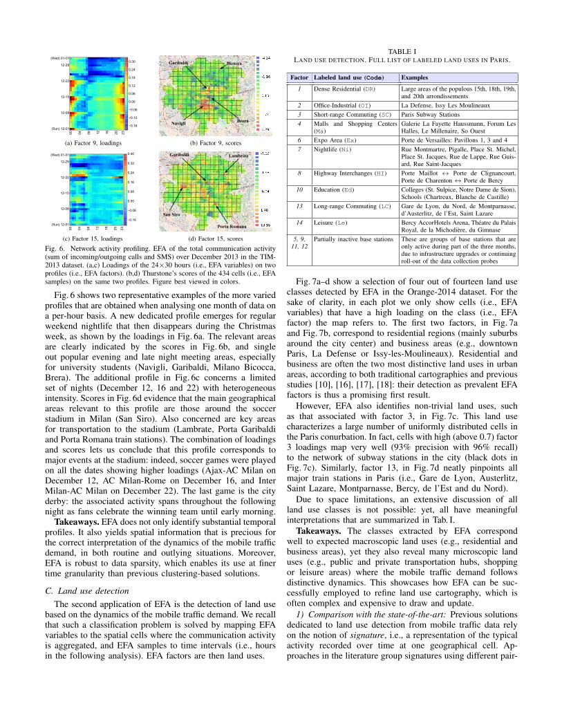
Fig. 6. Network activity profiling. EFA of the total communication activity(sum of incoming/outgoing calls and SMS) over December 2013 in the TIM-2013 dataset. (a,c) Loadings of the 24×30 hours (i.e., EFA variables) on twoprofiles (i.e., EFA factors). (b,d) Thurstone’s scores of the 434 cells (i.e., EFAsamples) on the same two profiles. Figure best viewed in colors.

Fig. 6 shows two representative examples of the more variedprofiles that are obtained when analysing one month of data ona per-hour basis. A new dedicated profile emerges for regularweekend nightlife that then disappears during the Christmasweek, as shown by the loadings in Fig. 6a. The relevant areasare clearly indicated by the scores in Fig. 6b, and singleout popular evening and late night meeting areas, especiallyfor university students (Navigli, Garibaldi, Milano Bicocca,Brera). The additional profile in Fig. 6c concerns a limitedset of nights (December 12, 16 and 22) with heterogeneousintensity. Scores in Fig. 6d evidence that the main geographicalareas relevant to this profile are those around the soccerstadium in Milan (San Siro). Also concerned are key areasfor transportation to the stadium (Lambrate, Porta Garibaldiand Porta Romana train stations). The combination of loadingsand scores lets us conclude that this profile corresponds tomajor events at the stadium: indeed, soccer games were playedon all the dates showing higher loadings (Ajax-AC Milan onDecember 12, AC Milan-Rome on December 16, and InterMilan-AC Milan on December 22). The last game is the cityderby: the associated activity spans throughout the followingnight as fans celebrate the winning team until early morning.

Takeaways. EFA does not only identify substantial temporalprofiles. It also yields spatial information that is precious forthe correct interpretation of the dynamics of the mobile trafficdemand, in both routine and outlying situations. Moreover,EFA is robust to data sparsity, which enables its use at finertime granularity than previous clustering-based solutions.

C. Land use detectionThe second application of EFA is the detection of land use

based on the dynamics of the mobile traffic demand. We recallthat such a classification problem is solved by mapping EFAvariables to the spatial cells where the communication activityis aggregated, and EFA samples to time intervals (i.e., hoursin the following analysis). EFA factors are then land uses.

TABLE ILAND USE DETECTION. FULL LIST OF LABELED LAND USES IN PARIS.

Factor Labeled land use (Code) Examples

1 Dense Residential (DR) Large areas of the populous 15th, 18th, 19th,and 20th arrondissements

2 Office-Industrial (OI) La Defense, Issy Les Moulineaux3 Short-range Commuting (SC) Paris Subway Stations4 Malls and Shopping Centers

(Ma)Galerie La Fayette Haussmann, Forum LesHalles, Le Millenaire, So Ouest

6 Expo Area (Ex) Porte de Versailles: Pavillons 1, 3 and 47 Nightlife (Ni) Rue Montmartre, Pigalle, Place St. Michel,

Place St. Jacques, Rue de Lappe, Rue Guis-ard, Rue Saint-Jacques

8 Highway Interchanges (HI) Porte Maillot ↔ Porte de Clignancourt,Porte de Charenton ↔ Porte de Bercy

10 Education (Ed) Colleges (St. Sulpice, Notre Dame de Sion),Schools (Chartreux, Blanche de Castille)

13 Long-range Commuting (LC) Gare de Lyon, du Nord, de Montparnasse,d’Austerlitz, de l’Est, Saint Lazare

14 Leisure (Le) Bercy AccorHotels Arena, Theatre du PalaisRoyal, de la Michodiere, du Gimnase

5, 9,11, 12

Partially inactive base stations These are groups of base stations that areonly active during part of the three months,due to infrastructure upgrades or continuingroll-out of the data collection probes

Fig. 7a–d show a selection of four out of fourteen land useclasses detected by EFA in the Orange-2014 dataset. For thesake of clarity, in each plot we only show cells (i.e., EFAvariables) that have a high loading on the class (i.e., EFAfactor) the map refers to. The first two factors, in Fig. 7aand Fig. 7b, correspond to residential regions (mainly suburbsaround the city center) and business areas (e.g., downtownParis, La Defense or Issy-les-Moulineaux). Residential andbusiness are often the two most distinctive land uses in urbanareas, according to both traditional cartographies and previousstudies [10], [16], [17], [18]: their detection as prevalent EFAfactors is thus a promising first result.

However, EFA also identifies non-trivial land uses, suchas that associated with factor 3, in Fig. 7c. This land usecharacterizes a large number of uniformly distributed cells inthe Paris conurbation. In fact, cells with high (above 0.7) factor3 loadings map very well (93% precision with 96% recall)to the network of subway stations in the city (black dots inFig. 7c). Similarly, factor 13, in Fig. 7d neatly pinpoints allmajor train stations in Paris (i.e., Gare de Lyon, Austerlitz,Saint Lazare, Montparnasse, Bercy, de l’Est and du Nord).

Due to space limitations, an extensive discussion of allland use classes is not possible: yet, all have meaningfulinterpretations that are summarized in Tab. I.

Takeaways. The classes extracted by EFA correspondwell to expected macroscopic land uses (e.g., residential andbusiness areas), yet they also reveal many microscopic landuses (e.g., public and private transportation hubs, shoppingor leisure areas) where the mobile traffic demand followsdistinctive dynamics. This showcases how EFA can be suc-cessfully employed to refine land use cartography, which isoften complex and expensive to draw and update.

1) Comparison with the state-of-the-art: Previous solutionsdedicated to land use detection from mobile traffic data relyon the notion of signature, i.e., a representation of the typicalactivity recorded over time at one geographical cell. Ap-proaches in the literature group signatures using different pair-

(a) Factor (land use class) 1

La Defense

downtownParis

Issy-les-Moulineaux

(b) Factor (land use class) 2 (c) Factor (land use class) 3

Est

Nord

Saint Lazare

MontparnasseLyon

Bercy

Austerlitz

(d) Factor (land use class) 13

(e) Clusters 0, 1, 3, 6 (f) Clusters 2, 5, 7 (g) Cluster 4 (h) Clusters 36 and 41

Fig. 7. Land use detection. (a)-(d) EFA of the total communication activity (sum of incoming/outgoing calls and SMS) in the Orange-2014 dataset. Loadingsof the 1596 Voronoi cells (i.e., EFA variables) on four (out of fourteen) representative classes (i.e., EFA factors). (e)-(f) Signature clustering [18] on the totalcommunication activity (sum of incoming/outgoing calls and SMS) in the Orange-2014 dataset: Voronoi cell clusters that match our choice of EFA factors.Figure best viewed in colors.

00 04 08 12 16 20 23

(Sun) 11-3011-29

11-22

11-15

11-08

(Sat) 11-011.2

0.8

0.4

0.0

0.4

0.8

1.2

1.6

2.0

(a) Factor 1

00 04 08 12 16 20 23

(Sun) 11-3011-29

11-22

11-15

11-08

(Sat) 11-01 1.2

0.8

0.4

0.0

0.4

0.8

1.2

1.6

2.0

(b) Factor 2

00 04 08 12 16 20 23

(Sun) 11-3011-29

11-22

11-15

11-08

(Sat) 11-01 1.0

0.5

0.0

0.5

1.0

1.5

2.0

2.5

3.0

(c) Factor 3

00 04 08 12 16 20 23

(Sun) 11-3011-29

11-22

11-15

11-08

(Sat) 11-01 3.2

2.4

1.6

0.8

0.0

0.8

1.6

2.4

3.2

(d) Factor 13

Fig. 8. Land use detection. EFA of the total communication activity (sum ofincoming/outgoing calls and SMS) in the Orange-2014 dataset in November.Thurstone’s scores of the 91×24 hours (i.e., EFA samples) on a selection ofthe 16 classes (i.e., EFA factors). Figure best viewed in colors.

wise signature similarity measures and clustering algorithms.The resulting clusters of signatures are the land uses. Forour comparative evaluation, we consider median weeks (seeSec. V-B) as signatures, and measure their similarity via Pear-son correlation. Clustering is performed through linkage withan average distance criterion, using skewness minimization asthe stopping rule. This configuration is the most suitable forland use detection, according to comparative evaluations [18].

Fig. 7e-h portray some classes (i.e., signature clusters) gen-erated by the benchmark technique above. The match withEFA results is striking. E.g., Fig. 7e shows that signatureclusters 0, 1, 3 and 6 identify the same cells as EFA factor 1,i.e., residential suburban areas in the Paris region.

Interestingly, different clusters in the plot coincide withcells that have various loadings on the EFA factor (e.g.,see the similar geographical distribution of light and darkcolors in Fig. 7a and Fig. 7e): this means that the diversesignature clusters in Fig. 7e just capture different intensities ofa same phenomenon – in this case the actual preponderanceof residential users in the cell over other user types. Similarconsiderations hold for the remaining plots, in Fig. 7f-h. Infact, we found each EFA factor to correspond to 2-4 signatureclusters in most cases. Our conclusion is that EFA provides amore compact set of classes, grouping clusters that are akin;then, it allows in-depth intra-class analysis via loading values.

DR OI

SC

LC HI

SC

DR OI

Ma

DR OI

Ni

Fig. 9. Land use detection. Venn diagrams of the distribution of cells intopartially overlapping land uses (coded as in Tab. I). Mixed land uses arerepresented by the set intersections.

Takeaways. The quality of the proposed EFA classificationis equivalent to that granted by a dedicated state-of-the-art so-lution. In fact, the benchmark framework returns a much largerset of clusters that are often strongly related to each other interms of their underlying demand dynamics: however, suchinter-cluster relationships are unknown, and cumbersome toidentify a posteriori. EFA eases significantly the interpretationof results, as it returns a more concise set of classes that canbe further explored through loading analysis.

2) Advantages of EFA: Also under this problem formu-lation, scores can be leveraged to confirm and improve ourunderstanding of factors. More precisely, EFA returns scoresthat indicate the relevance of time (i.e., EFA samples) to eachclass (i.e., EFA factor). Thus, scores tell us when each land useclass shows an especially remarkable mobile communicationactivity5. This is not possible with any previous technique.

Fig. 8 shows the hourly scores during one months ofOrange-2014 data on a representative subset of land use classesdetected by EFA. We can observe that the suburban residentialareas of factor 1 have distinctive traffic patterns during theevening hours of the working days, in Fig. 8a. These are theonly areas of Paris where traffic surges between 8 pm and10 pm on Mondays to Fridays. As expected, the workinghours are most relevant to business areas in factor 2, shownin Fig. 8b: interestingly, morning hours seem more concernedthan afternoon ones. One can also easily detect that the typical

5The same considerations in footnote 4 apply here as well, and time seriesof cell scores are not simple time series of the aggregate mobile traffic volume.

working day spans from 8 am to 6-7 pm: these are the morningand afternoon commuting times when the subway stations offactor 3 experience exceptionally high loads, as displayed inFig. 8c. Train stations show a different temporal pattern, asthe most characteristic activity occurs during the afternooncommuting hours only. In all plots it is easy to spot anirregularity, due to a public holiday (Armistice, November 11).

A second major advantage of EFA is that loadings explainhow the activity in each geographical cell is related to allland uses at the same time. Thus, EFA naturally providesinformation on mixed land uses, i.e., city regions wheredifferent urban infrastructures merge. An example is providedin Fig. 9: set intersections in the Venn diagrams illustrate towhat extent land uses overlap in Paris. Significant areas ofmixed residential-business (DR-OI) nature exist, and they arefairly well served by short-commuting services (SC). Also,the same subway network (SC) links together all train stations(LC) as well as several major highway entry/exit nodes (HI).Malls and shopping centers (Ma) are uniformly distributedacross residential and office areas, whereas nightlife (Ni) onlythrives in densely populated regions of the city.

Retrieving similar information from the output of traditionalclustering-based solutions, which rigidly assign each cell toone land use, requires complex processing. This has only beenattempted recently, and with a small set of land uses [10].

Takeaways. EFA does not only identifies relevant land usesin the urban landscape. It also provides temporal knowledgethat helps interpreting them, and that immediately highlightshow special events affect one or more land uses. In addition,EFA loadings implicitly bear mixed land use information,which are not easily inferred with traditional approaches.

VI. CONCLUSIONS AND PERSPECTIVES

We proposed an original approach to the spatiotemporalclassification of mobile traffic data, which relies on Ex-ploratory Factor Analysis (EFA). Extensive tests with het-erogeneous real-world datasets demonstrate the versatility ofEFA, which provides a unifying framework to solve problemsthat have been studied in isolation in the literature, i.e., mobiletraffic profiling and land use detection. In both cases, EFAattains results that improve those of state-of-the-art solutions(e.g., the richer information of network activity profiles),or match them while yielding greater consistency (e.g., thebetter abstracted land use classes, where loadings can beleveraged for intra-class analysis). In addition, EFA providessupplementary knowledge (i.e., the geographical perspectiveof profiles and the temporal view of land uses) that provesparamount to the interpretation of the results, and eases tasksthat are otherwise complex to perform (e.g., the analysis ofper-hour temporal data, or the detection of mixed land uses).

EFA-based classification can find applications in data-drivennetwork operations, at multiple levels. The temporal structuresidentified by EFA expose non-trivial long-term dynamics inthe mobile traffic demand that are relevant to the allocation ofresources in, e.g., Cloud Radio Access Networks (C-RAN) [9].In addition, typical temporal profiles may serve as a basis forthe detection of anomalous network usages, and for predictingthe future demand in the context of anticipatory networking.In the spatial dimension, EFA classes neatly characterize thestrong geographical locality of mobile demand. They can thus

pave the way for cognitive network functions that aim atmigrating network resources geographically, or at dynamicallyconfiguring the network topology; such functions are espe-cially relevant to, e.g., Mobile Edge Computing (MEC) infras-tructures [9]. Overall, EFA-based classification is a potentialbrick for future big data-driven 5G systems [29].

VII. ACKNOWLEDGMENTS

The authors thank friends and colleagues in Milan and Pariswho helped interpreting the classification results. This workwas supported by the French National Research Agency grantANR-13-INFR-0005 ABCD, and by the EU FP7 ERA-NETprogram grant CHIST-ERA-2012 MACACO.

REFERENCES

[1] Cisco VNI Forecast, “Visual Networking Index: Global Mobile Data Traffic ForecastUpdate, 2015–2020,” 2016.

[2] M.Z. Shafiq, L. Ji, A. X. Liu, J. Wang, “Characterizing and Modeling Internet TrafficDynamics of Cellular Devices,” ACM SIGMETRICS, 2011.

[3] D. Willkomm, S. Machiraju, J. Bolot, A. Wolisz, “Primary Users in CellularNetworks: A Large-Scale Measurement Study,” IEEE DySPAN, 2008.

[4] M.Z. Shafiq, L. Ji, A.X. Liu, J. Pang, S. Venkataraman, J. Wang, “A First Look atCellular Network Performance during Crowded Events,” ACM SIGMETRICS, 2013.

[5] U. Paul, A.P. Subramanian, M.M. Buddhikot, S.R. Das, “Understanding TrafficDynamics in Cellular Data Networks,” IEEE INFOCOM, 2011.

[6] R. Keralapura, A. Nucci, Z.-L. Zhang, L. Gao, “Profiling Users in a 3G NetworkUsing Hourglass Co-Clustering,” ACM MobiCom, 2010.

[7] D. Naboulsi, M. Fiore, S. Ribot, R. Stanica, “Large-scale Mobile Traffic Analysis:A Survey,” IEEE Communications Surveys & Tutorials, 18(1), 2016.

[8] R.W. Thomas, L.A. Da Silva, A.B. MacKenzie, “Cognitive networks,” IEEEDySPAN, 2005.

[9] H. Assem, T. Sandra Buda, L. Xu, “Initial use cases, scenarios and requirements,”H2020 5G-PPP CogNet, Deliverable D2.1, 2015.

[10] M. Lenormand, M. Picornell, O.G. Cantu-Ros, T. Louail, R. Herranz, M.Barthelemy, E. Frıas-Martınez, M. San Miguel, J.J. Ramasco, “Comparing andmodelling land use organization in cities,” Royal Society Open Science, 2, 2016.

[11] D. Goergen, V. Mendiratta, R. State, T. Engel, “Identifying Abnormal Patterns inCellular Communication Flows,” ACM IPTComm, 2013.

[12] F. Calabrese, F.C. Pereira, G. Di Lorenzo, L. Liu, C. Ratti, “The Geography of Taste:Analyzing Cell-Phone Mobility and Social Events,” Pervasive Computing, 2010.

[13] J.P. Bagrow, D. Wang, A.-L. Barabasi, “Collective Response of Human Populationsto Large-Scale Emergencies,” PLoS ONE, 6(3), 2011.

[14] D. Naboulsi, R. Stanica, M. Fiore, “Classifying Call Profiles in Large-scale MobileTraffic Datasets,” IEEE INFOCOM, 2014.

[15] I. Trestian, S. Ranjan, A. Kuzmanovic, A. Nucci, “Measuring Serendipity: Connect-ing People, Locations and Interests in a Mobile 3G Network,” ACM IMC, 2009.

[16] J.L. Toole, M. Ulm, M.C. Gonzalez, D. Bauer, “Inferring Land Use from MobilePhone Activity,” ACM UrbComp, 2012.

[17] B. Cici, M. Gjoka, A. Markopoulou, C.T. Butts, “On the Decomposition of CellPhone Activity Patterns and their Connection with Urban Ecology,” ACM MobiHoc,2015.

[18] A. Furno, R. Stanica, M. Fiore, “A Comparative Evaluation of Urban FabricDetection Techniques Based on Mobile Traffic Data,” IEEE/ACM ASONAM, 2015.

[19] C. Spearman, “General Intelligence Objectively Determined and Measured,” TheAmerican Journal of Psychology, 15(2), 1904.

[20] L.R. Fabrigar, D.T. Wegener, R.C. MacCallum, E.J. Strahan, “Evaluating the Use ofExploratory Factor Analysis in Psychological Research,” Psychological Methods,4(3), 1999.

[21] S.A. Mulaik, Foundations of Factor Analysis, CRC Press, 2009.[22] D.N. Lawley, “The Estimation of Factor Loadings by the Method of Maximum

Likelihood,” Proc. of the Royal Society of Edinburgh, 60(1), 1940.[23] I.T. Jolliffe, “Principal Component Analysis and Factor Analysis,” Principal Com-

ponent Analysis, Springer Series in Statistics, 2002.[24] J.C.F. de Winter, D. Dodou, “Common Factor Analysis versus Principal Component

Analysis: A Comparison of Loadings by Means of Simulations,” Communicationsin Statistics - Simulation and Computation, 45(1), 2016.

[25] H.F. Kaiser, J. Rice, “Little Jiffy, Mark IV,” Educational and PsychologicalMeasurement, 34, 1974.

[26] J.L. Horn, “A Rationale and Test for the Number of Factors in Factor Analysis,”Psychometrika, 30(2), 1965.

[27] H.F. Kaiser, “The VARIMAX Criterion for Analytic Rotation in Factor Analysis,”Psychometrika, 23(3), 1958.

[28] L.L. Thurstone, “The vectors of mind”, University of Chicago Press, 1935.[29] K. Zheng, Z. Yang, K. Zhang, P. Chatzimisios, K. Yang, W. Xiang, “Big data-driven

optimization for mobile networks toward 5G,” IEEE Network, 30(1), 2016.