NSEL Report SeriesReport No. NSEL-020

November 2009

Joint Shear Behavior ofJoint Shear Behavior ofReinforced Concrete Beam-Column Connections

subjected to Seismic Lateral Loading

Jaehong Kimand

James M. LaFave

Department of Civil and Environmental EngineeringUniversity of Illinois at Urbana-Champaign

NEWMARK STRUCTURAL ENGINEERING LABORATORY

UILU-ENG-2009-1808

ISSN: 1940-9826

© The Newmark Structural Engineering Laboratory

The Newmark Structural Engineering Laboratory (NSEL) of the Department of Civil and Environmental Engineering at the University of Illinois at Urbana-Champaign has a long history of excellence in research and education that has contributed greatly to the state-of-the-art in civil engineering. Completed in 1967 and extended in 1971, the structural testing area of the laboratory has a versatile strong-floor/wall and a three-story clear height that can be used to carry out a wide range of tests of building materials, models, and structural systems. The laboratory is named for Dr. Nathan M. Newmark, an internationally known educator and engineer, who was the Head of the Department of Civil Engineering at the University of Illinois [1956-73] and the Chair of the Digital Computing Laboratory [1947-57]. He developed simple, yet powerful and widely used, methods for analyzing complex structures and assemblages subjected to a variety of static, dynamic, blast, and earthquake loadings. Dr. Newmark received numerous honors and awards for his achievements, including the prestigious National Medal of Science awarded in 1968 by President Lyndon B. Johnson. He was also one of the founding members of the National Academy of Engineering.

Contact:

Prof. B.F. Spencer, Jr. Director, Newmark Structural Engineering Laboratory 2213 NCEL, MC-250 205 North Mathews Ave. Urbana, IL 61801 Telephone (217) 333-8630 E-mail: bfs@illinois.edu

This technical report is based on the first author’s doctoral dissertation of the same title, which was completed by January 2008. The second author served as the dissertation advisor for this work. Partial financial support for this research was provided to the first author in the form of a Burt & Erma Lewis Graduate Fellowship in the Department of Civil and Environmental Engineering at the University of Illinois, as well as by a Portland Cement Association Educational Foundation Fellowship. The authors would also like to acknowledge the collaborative assistance provided by Junho Song and Won-Hee Kang in making some of the calculations related to the Bayesian parameter estimation procedure. The cover photographs are used with permission. The Trans-Alaska Pipeline photograph was provided by Terra Galleria Photography (http://www.terragalleria.com/).

ABSTRACT

Beam-column connections have been identified as potentially one of the weaker components of reinforced concrete moment resisting frames subjected to seismic lateral loading. Well-established knowledge of RC joint shear behavior is necessary because severe damage within a joint panel may trigger deterioration of the overall performance of RC beam-column connections or frames. However, despite the importance of understanding RC joint shear behavior, a consensus on the ways in which some parameters affect joint shear strength has not been reached. In addition, there has generally been no accepted behavior model for RC joint shear stress vs. joint shear strain. Therefore, in this research a more systematic understanding of RC joint shear behavior has been achieved by completing the following tasks: construction of an extensive experimental database, characterization of RC joint shear behavior, and development of RC joint shear strength models and proposed joint shear behavior models. An extensive experimental RC beam-column connection database (of 341 subassemblies in total) was constructed and classified by governing failure mode sequence, in-plane geometry, out-of-plane geometry, and joint eccentricity. All included subassemblies were made at a minimum of one-third scale, and all used conventional types of reinforcement anchorages. RC joint shear behavior was described as an envelope curve by connecting key points displaying the most distinctive stiffness changes. The first point indicates initiation of diagonal cracking within a joint panel, the second point results from yielding of reinforcement, and the third point corresponds to maximum response. An RC joint shear strength model was then developed using the experimental database in conjunction with the Bayesian parameter estimation method. A simple and unified joint shear deformation model (at maximum response) was also developed, following the same procedure used to develop the simple and unified joint shear strength model. Full RC joint shear behavior models were constructed by employing the Bayesian method at each key point and also by adjusting the simple and unified joint shear strength and deformation models for maximum response. Finally, the Parra-Montesinos and Wight model was modified to improve its reliability by updating the key relation between principal strain ratio and joint shear deformation.

TABLE OF CONTENTS

CHAPTER 1: INTRODUCTION.................................................................................... 1

1.1 Background............................................................................................................... 1 1.2 Research scope and objective ................................................................................... 1 1.3 Chapter description ................................................................................................... 2

CHAPTER 2: BACKGROUND INFORMATION OF RC JOINT SHEAR BEHAVIOR....................................................................................................................... 4

2.1 Code recommendations............................................................................................. 4 2.1.1 ACI 352R-02 and ACI 318-05........................................................................... 4 2.1.2 AIJ 1999............................................................................................................. 5 2.1.3 NZS 3101: 1995................................................................................................. 6

2.2 Experimental investigations – test database ............................................................. 7 2.3 Analytical examinations............................................................................................ 8

CHAPTER 3: EXPERIMENTAL DATABASE .......................................................... 14

3.1 Database construction criteria................................................................................. 14 3.2 Minimum confinement within a joint panel............................................................ 16 3.3 ACI design guidelines with respect to joint shear strength..................................... 18

3.3.1 ACI design guidelines – general issues ........................................................... 18 3.3.2 Ash ratio and spacing ratio................................................................................ 19 3.3.3 Column depth or development length ratio ..................................................... 20 3.3.4 ACI 352R-02 joint shear strength definition ................................................... 21

CHAPTER 4: CHARACTERIZATION OF RC JOINT SHEAR BEHAVIOR ...... 24

4.1 Key points of joint shear behavior .......................................................................... 24 4.2 Diagonal cracking within a joint panel (point A) ................................................... 25 4.3 Assessment of influence parameters (at points B and C) ....................................... 27

4.3.1 Trends for the basic dataset.............................................................................. 27 4.3.1.1 Concrete compressive strength ................................................................. 28

4.3.1.2 RC joint panel geometry ............................................................................... 29 4.3.1.3 Reinforcement index................................................................................. 29 4.3.1.4 Column axial compression........................................................................ 31 4.3.1.5 Bond demand level of longitudinal reinforcement ................................... 31 4.3.1.6 Joint shear stress vs. joint shear strain ...................................................... 33

4.3.2 Insufficient joint confinement.......................................................................... 34 4.3.3 Out-of-plane geometry..................................................................................... 38 4.3.4 Joint eccentricity .............................................................................................. 39 4.3.5 Descending slope ............................................................................................. 39 4.3.6 Assessment summary....................................................................................... 40

CHAPTER 5: RC JOINT SHEAR STRENGTH MODEL ........................................ 66

5.1 Probabilistic methodology ...................................................................................... 66 5.2 RC Joint shear strength model ................................................................................ 69

5.2.1 Procedural framework- basic dataset ............................................................... 69 5.2.2 RC joint shear strength model for reduced dataset .......................................... 73 5.2.3 Unified RC joint shear strength model for total database except subassemblies with 0 in Ash ratio...................................................................................................... 75

5.3 Performance evaluation: Joint shear strength models............................................. 80 5.4 Subassemblies with no joint transverse reinforcement........................................... 81 5.5 Specific non-standard conditions in RC beam-column connections ...................... 82

5.5.1 Subassemblies with anchorage plates .............................................................. 82 5.5.2 Fiber-reinforced concrete................................................................................. 83

5.6 Modified ACI 352R-02 joint shear strength model ................................................ 85 5.6.1 First approach in the modification of the ACI 352 model ............................... 86 5.6.2 Second approach in the modification of the ACI 352R-02 model................... 87

CHAPTER 6: RC JOINT SHEAR BEHAVIOR MODEL....................................... 100

6.1 Joint shear deformation model: maximum response (point C)............................. 100 6.1.1 Joint shear deformation model: Basic dataset and reduced dataset ............... 101 6.1.2 Joint shear deformation model (at maximum response): Total database (except subassemblies with 0 in Ash ratio) .......................................................................... 104

6.2 Joint shear behavior model at point B................................................................... 108 6.2.1 Joint shear stress model: point B ................................................................... 108 6.2.2 Joint shear strain model: point B ................................................................... 110

6.3 Joint shear behavior model at point A .................................................................. 112 6.3.1 Joint shear stress model: point A ................................................................... 112 6.3.2 Joint shear strain model: point A ................................................................... 114

6.4 Joint shear behavior model for descending (post peak) response......................... 117 6.4.1 Joint shear stress model: point D ................................................................... 117 6.4.2 Joint shear strain model: point D ................................................................... 118

6.5 Summary of the developed joint shear behavior models ...................................... 120 6.6 Subassemblies with no joint transverse reinforcement......................................... 123 6.7 Performance evaluation: Joint shear behavior ...................................................... 124

6.7.1 FEMA 356 joint shear model......................................................................... 124 6.7.2 Teraoka and Fujii model ................................................................................ 126 6.7.3 Parra-Montesinos and Wight model .............................................................. 128 6.7.4 Modified Compression Field Theory (MCFT) .............................................. 131

6.8 Modified Parra-Montesinos and Wight model ..................................................... 136 6.9 Summary of RC joint shear behavior models ....................................................... 140

CHAPTER 7: CONCLUSIONS AND RECOMMENDATIONS............................. 164

7.1 Conclusions........................................................................................................... 164 7.1.1 Construction of experimental database.......................................................... 164 7.1.2 Characterization of joint shear behavior ........................................................ 165

7.1.3 Development of joint shear strength models ................................................. 166 7.1.4 Complete joint shear stress vs. strain prediction model................................. 167

7.2 Recommendations for future research .................................................................. 169

REFERENCES.............................................................................................................. 170

APPENDIX A: EXPERIMENTAL DATABASE ...................................................... 185

APPENDIX B: JOINT SHEAR BEHAVIOR PLOT RESULTS............................. 192

1

Chapter 1

INTRODUCTION

1.1 Background

Reinforced concrete moment resisting frames (RCMRF) are structural systems designed to ensure proper energy dissipation capacity and lateral stability when subjected to seismic lateral loading. In this design philosophy, the so-called “strong-column / weak-beam” concept is recommended and elastic behavior of the joints and columns of RCMRF is desirable. Beam-column connections have been identified as potentially one of the weaker components when RCMRF is subjected to seismic lateral loading. Since the mid-1960s, numerous experimental tests and analytical studies have been conducted to investigate the performance of reinforced concrete (RC) beam-column connections subjected to lateral earthquake loading. When only the flexural strength of well-detailed longitudinal beams limits overall response, RC beam-column connections typically display ductile behavior (with the joint panel region essentially remaining elastic). The failure mode wherein the beams form hinges is usually considered to be the most desirable for maintaining good global energy-dissipation without severe degradation of capacity at the connections. On the other hand, RC beam-column connections can exhibit less robust behavior when severe damage is concentrated within the joint panel. Therefore, understanding joint shear behavior is important toward controlling the overall performance of RC beam-column connections and frames.

In various countries (the United States, New Zealand, Japan, Republic of Korea, etc.), many researchers have tried several approaches to improve understanding of RC joint shear behavior. Influence parameters on joint shear behavior have been examined using collected experimental test results and analytical procedures. However, there is still no consensus about the effect of some parameters on joint shear strength (and/or joint shear deformation). Thus, some design considerations for joint shear strength have not yet been fully codified due to insufficient conclusive information. In addition, there is no generally accepted joint shear stress vs. joint shear strain prediction model that can describe the complete joint shear behavior of diverse types of RC beam-column connections.

1.2 Research scope and objective

The overall objective of this research is to provide a more profound understanding of joint shear behavior across diverse types of RC beam-column connections subjected to seismic lateral loadings. To achieve this overall objective, the following specific research tasks have been completed.

• An extensive experimental database of RC beam-column connection subassembly tests was constructed by employing consistent inclusion criteria, and it was further classified by governing failure mode, in-plane geometry, out-of-plane geometry, and joint eccentricity.

2

• The minimum amount of joint transverse reinforcement was identified to maintain proper joint confinement, and the determined cut-off point was confirmed by examining the role of ACI design guidelines with respect to joint shear strength.

• RC joint shear stress vs. joint shear strain behavior was characterized by identifying key points (displaying the most distinct stiffness changes) and by assessing possible influence parameters (describing diverse conditions of RC beam-column connections) at the identified key points.

• A procedural framework was established to develop an RC joint shear strength model using basic types of RC beam-column connections (subassemblies maintaining proper joint confinement with no out-of-plane members and no joint eccentricity), in conjunction with a Bayesian parameter estimation method.

• Unified joint shear strength and joint shear deformation models were proposed for the maximum response of diverse types of RC beam-column connections. The performance of the proposed joint shear strength and deformation models was evaluated by comparison with deterministic models proposed by codes, recommendations, and other researchers.

• RC joint shear stress vs. joint shear strain behavior models were constructed by the Bayesian parameter estimation method for each identified key point and by adjusting the simple and unified joint shear strength and deformation models suggested for maximum response. To construct complete RC joint shear behavior models, a descending response (post peak) is also considered.

• In the final stage of this research, a joint shear behavior model previously proposed by Parra-Montesinos and Wight was modified to improve model reliability and to enhance its application to diverse types of RC beam-column connections.

1.3 Chapter description

This report presents a “Ph.D. thesis” dissertation to achieve the suggested objective explained above, and it consists of seven chapters and 2 appendices.

Chapter 2 provides a literature review for prior research work on the joint shear behavior of RC beam-column connections subjected to seismic lateral loading.

Chapter 3 introduces the constructed database of experimental subassemblies and determines the minimum amount of RC joint transverse reinforcement to maintain proper joint confinement.

Chapter 4 presents the characterization of RC joint shear stress vs. joint shear strain behavior by the following procedure: identification of key points in joint shear behavior,

3

selection of possible influence parameters, and assessment of influence parameters on joint shear behavior. Furthermore, the effects of insufficient joint confinement, out-of-plane geometry, joint eccentricity, and descending slope on joint shear behavior are also examined.

Chapter 5 addresses issues related to RC joint shear strength. The Bayesian parameter estimation method is first introduced. The procedure to develop the simple and unified joint shear strength model, which can be applicable to diverse types of RC beam-column connections, is then presented. The performance of the suggested model is evaluated by comparison with other deterministic joint shear strength models. Discussion about the following conditions are also provided: application of the suggested model to subassemblies with no joint transverse reinforcement, the effect of using anchorage plates for longitudinal beam reinforcement on joint shear strength, and the effect of using fiber-reinforced concrete on joint shear strength. Finally, the ACI 352R-02 joint shear strength model is modified to adjust to improve model reliability.

Chapter 6 examines issues related to overall RC joint shear behavior. A procedure to develop a simple and unified joint shear deformation model at the peak stress is first proposed. At other key points, RC joint shear behavior models are then constructed by the Bayesian parameter estimation method and also by adjusting the simple and unified joint shear strength and deformation models. Discussion about the application of the simple and unified joint shear behavior model for subassemblies with no joint transverse reinforcement is presented. Performance of the suggested overall joint shear behavior model is evaluated by comparison with other deterministic joint shear behavior models. In the final stage, the Parra-Montesinos and Wight model is modified to improve model reliability and enhance model application.

Chapter 7 summarizes the key conclusions from this research and also suggests recommendations for the direction of future research work.

Finally, Appendices A and B present the detailed information about the constructed experimental database and joint shear stress vs. joint shear strain plot results, respectively.

4

Chapter 2

BACKGROUND INFORMATION OF RC JOINT SHEAR BEHAVIOR

The geometric categories of RC beam-column connections are a function of in-plane geometry, out-of-plane geometry (transverse beam(s) and/or slab(s)), and joint eccentricity. Figure 2.1 displays various types of RC beam-column connection subassemblies according to in-plane geometry. An interior connection has two longitudinal beams with a continuous column, an exterior connection has one longitudinal beam with a continuous column, and a knee connection has one longitudinal beam with a discontinuous column. Hanson and Connor (1967) first suggested a quantitative definition of RC joint shear, namely that it could be determined from a free-body diagram at mid-height of a joint panel. For example, Figure 2.2 shows joint shear at mid-height of the joint panel for a typical interior connection subassembly. Paulay et al. (1978) described qualitative shear-resistance mechanism(s) for a joint panel, which consist of some combination of a concrete strut and/or a truss. Shear-resistance provided by the concrete strut mechanism comes from force transfer to the joint panel by bearing from concrete compression zones of adjacent beam(s) and column(s), whereas shear-resistance provided by the truss mechanism primarily comes from force transfer to the joint panel via bond between reinforcement and surrounding concrete, which are shown in Figure 2.3.

Starting from the key studies noted above, much research has subsequently been performed to improve the understanding of RC joint shear behavior. In this chapter, important previous work is summarized into three main categories, namely, code recommendations, experimental investigations, and analytical examinations.

2.1 Code recommendations

2.1.1 ACI 352R-02 and ACI 318-05

For modern RC beam-column connections (maintaining proper confinement within a joint panel), ACI-ASCE Committee 352 (“Joints and Connections in Monolithic Concrete Structures”) has defined a nominal joint shear strength; that is:

cj'cACIn hbfV γ= (2.1)

where ACIγ is the joint shear strength factor, 'cf is the specified concrete compressive

strength, jb is the effective joint shear width, and ch is the column depth. The joint shear strength factor is determined as a function of the number of vertical faces around the joint panel effectively confined (equal to or above 0.75 in beam-to-column width ratio) by longitudinal and transverse beam(s), which is summarized in Table 2.1.

5

Table 2.1 Joint shear strength factor (ACI 352R-02) Classification ACIγ (MPa0.5) A. Joints with a continuous column A.1 Joints effectively confined on all four vertical faces 1.67 A.2 Joints effectively confined on three vertical faces or on two opposite vertical faces 1.25

A.3 Other cases 1.00 B. Joints with a discontinuous column B.1 Joints effectively confined on all four vertical faces 1.25 B.2 Joints effectively confined on three vertical faces or on two opposite vertical faces 1.00

B.3 Other cases 0.67

Effective joint shear width is determined as the smallest of three values; that is:

∑++

= )b,2

mhb,

2bb

(smallestb cc

bcb

j (2.2)

In Equation (2.2), bb is the beam width, cb is the column width, and m is the slope to define the effective width of joint transverse to the direction of shear. m should be 0.3 when the eccentricity between the beam centerline and the column centroid exceeds 8bc and m should be 0.5 for other cases. The term 2mhc should not be taken larger than the extension of the column beyond the edge of the beam. The average of beam and column widths usually governs the effective ACI 352R-02 joint shear width ( jb ) for RC beam-column connections without joint eccentricity.

ACI Committee 318 (“Building Code Requirements for Structural Concrete (ACI 318-05) and Commentary (ACI 318R-05)”) has generally accepted a similar joint shear design philosophy to that of ACI 352R-02 except for a few points. First, ACI 318-05 does not explicitly consider column discontinuity in determining the joint shear strength factor; exterior and knee joints just have the same joint shear strength factor for the same condition of out-of-plane members. Second, their effective joint shear width is determined as the smaller of two values; that is:

)x2b,hb(smallerb bcbj ++= (2.3)

where x is the smaller of the distances from beam face to column face. Column width usually governs the ACI 318-05 effective joint shear width ( jb ) for RC beam-column connections without joint eccentricity.

2.1.2 AIJ 1999

AIJ 1999 (“Design guidelines for earthquake resistant reinforced concrete building based on ultimate strength concept and commentary”) has recommended a nominal

6

joint shear strength in the form of Equation (2.4); that is:

jjjj DbFkV φ= (2.4)

In Equation (2.4), k is the factor dependent on the shape of in-plane geometry (1.0 for interior connections, 0.7 for exterior connections and T-shape top story joints, and 0.4 for corner knee connections); φ is the factor for the effect of out-of-plane geometry (1.0 for joints with transverse beams on both sides and 0.85 for other types of joints); jF is the standard value of the joint shear strength (as a function of concrete compressive strength); jb is the effective joint shear width; and jD is the effective column depth.

The standard value of the joint shear strength ( jF ) is suggested as Equation (2.5); that is:

7.0cj )'f(8.0F ×= (2.5)

The effective joint width ( jb ) is defined as 2a1abj bbbb ++= ( 1ab , 2ab : the smaller of one-quarter of column depth and one-half of distance between beam and column face on either side of beam). Finally, the effective joint shear depth ( jD ) is simply defined as the column depth for an interior connection, or the projected development length of anchored beam bars with 90 degree hooks for exterior and knee joints.

2.1.3 NZS 3101: 1995

NZS 3101: 1995 (“Concrete Structures Standard”) has suggested the design joint shear strength as Equation (2.6); that is:

cjjj hbvV = (2.6)

where jv is the joint shear stress, jb is the effective joint shear width, and ch is the column depth.

Joint shear stress is defined as Equation (2.7); that is:

*sby

jhjy'c

jAf

Af

6f

vα

= (2.7)

In Equation (2.7), α is the parameter considering column axial load; jyf is the yield stress of horizontal joint transverse reinforcement; jhA is the total cross-sectional area of horizontal joint transverse reinforcement; byf is the yield stress of longitudinal beam

reinforcement; and *sA is the greater of the area of top or bottom beam reinforcement

passing through the joint (excluding bars in an effective tension flange). The computed

7

joint shear stress should not exceed 'cf2.0 .

The parameter ( α ) considering column axial load is computed as Equation (2.8-1) and (2.8-2); that is:

g'

c

*j

Af

NC6.14.1 −=α (Interior connections) (2.8-1)

⎟⎟⎟

⎠

⎞

⎜⎜⎜

⎝

⎛−β=α

g'

c

j

Af

NC7.0 (Exterior and knee connections) (2.8-2)

NZS 3101:1995 says that jC is introduced to proportionally allocate the beneficial effects of axial compression load to the 2 principal directions of the lateral design force ( jC is 1.0 for unidirectional joints and symmetrical two-way frames subject to axial tension, and jC is 0.5 for symmetrical two-way frames subject to axial compression); β is the area ratio of compression to tension beam reinforcement; N is the column axial load (positive value for axial compression and negative value for axial tension); and gA is the column cross-sectional area.

Finally, the effective joint shear width ( jb ) is the smaller of cb and cb h5.0b + . For RC beam-column connections without joint eccentricity, the effective joint shear width is generally governed by column width.

2.2 Experimental investigations – test database

Several researchers have investigated RC joint shear behavior based on their constructed experimental databases for RC beam-column connection subassemblies. In their constructed databases, some experimental subassemblies experienced joint shear failure either in conjunction with or without yielding of beam reinforcement, which is referred to as “BJ” and “J” failures, while, some experimental subassemblies experienced only beam flexural failure, which is referred to as “B” failure. For example, Kitayama et al. (1991) examined 15 interior “BJ” failures and 19 interior “J” failures from experiments conducted by them and by others. They reported two findings related to joint shear strength. First, joint shear strength seemed to be independent of column axial load, and second, joint shear strength was not enhanced by an increase in the amount of joint transverse reinforcement when the dimensionless joint transverse reinforcement ratio (total area of joint transverse reinforcement, located in the loading direction and placed between the top and bottom beam reinforcement, divided by the product of column width and the distance between the compressive and tensile resultants of the section) was already above 0.4%.

Bonacci and Pantazoupoulou (1993) collected data from experiments consisting of 34 interior “BJ” failures and 16 interior “J” failures. In collecting the experimental data, there was no restriction on the amount (how much or how little) of joint transverse

8

reinforcement. They indicated that column axial load has no coherent influence on joint shear strength. By calculating the potential contribution of joint transverse reinforcement to joint shear strength, they suggested that the participation of joint transverse reinforcement in the shear-resistance mechanism can be significant. Goto and Joh (1996) collected data from 52 experimental interior “BJ” failures and 23 interior “J” failures, again with no limitation on the amount of joint transverse reinforcement. According to their examination, joint shear strength was dependent on concrete compressive strength, and joint transverse reinforcement also somewhat affected joint shear strength. Kamimura et al. (2000) collected data from 87 interior joint tests. In this collected data, the governing failure modes were beam flexural failure, “BJ” failures, and “J” failures. As in other previous research, there was no restriction on the amount of joint transverse reinforcement when collecting the data. They reported that the amount of joint transverse reinforcement used in a frame structure had little influence on the shear strength and joint deformation of interior connections.

Kitayama (1992) proposed a tri-linear shear stress vs. shear strain envelope curve for RC joint shear behavior by defining joint shear moduli based on 11 interior “BJ” failures and 3 interior “J” failures (that again had no restriction on the amount of joint transverse reinforcement). To determine the shear moduli after diagonal cracks occurred in the joint panel, the following were considered: concrete compressive strength, joint transverse reinforcement, column reinforcement, column axial load, and lateral confinement by transverse beams and/or slabs. Similar to the suggestion of Kitayama (1992), Teraoka and Fujii (2000) also proposed an envelope curve of joint shear behavior, which consisted of four line segments. In their suggestion, joint shear stress (at maximum response) follows AIJ 1999 and joint shear strain at key transition points are fixed regardless of the diversity of joint panels. The proposed models of Kitayama (1992) and Teraoka and Fujii (2000) are certainly questionable for application to cases not covered by their collected experimental data, and could perhaps not even be the best for use with their respective own databases.

2.3 Analytical examinations

Hwang and Lee (1999, 2000) developed a softened strut-and-tie model to predict RC joint shear strength for both interior and exterior connections. This softened strut-and-tie model satisfies equilibrium, compatibility, and constitutive relations for cracked reinforced concrete. In order to satisfy these principles of mechanics, however, the distinct advantage in simplicity of a strut-and-tie model is lost in their proposed version. Their model was validated for collected experimental specimens (63 exterior and 56 interior connections) without any restriction on joint transverse reinforcement (and governing modes included beam flexural failures, “BJ” failures, and “J” failures).

More recently, Attaalla (2004) proposed an analytical equation to predict joint shear strength for interior and exterior connections. The analytical equation was developed from assuming a stress distribution around the joint panel that satisfied equilibrium, and also considering a compression-softening phenomenon associated with cracked reinforced concrete. The considered parameters in the proposed equation were axial force in the beam, axial force in the column, joint reinforcement ratio in the longitudinal

9

direction of the joint, joint reinforcement ratio in the transverse direction of the joint, and geometry. To validate the proposed equation, 69 exterior and 61 interior joint tests were used. In this collected data, the governing failure modes were “BJ” and “J” failures, and there was no limitation about the amount of joint transverse reinforcement. Shiohara (2004) proposed a mathematical model to determine the joint shear strength of interior, exterior, and knee connections. In this suggestion, the so-called “quadruple flexural resistance” within a joint panel played an important role in defining joint shear failures. Joint shear strength was determined from satisfying force equilibrium in four rigid segments within the joint panel. This proposed mathematical model was not validated based on collected experimental data.

Murakami et al. (2000) proposed a joint shear strength model for only interior connections with no out-of-plane members and no joint eccentricity. In this model, regression analysis was performed to develop a joint shear strength model by considering concrete compressive strength. Russo and Somma (2004) have recently suggested a joint shear strength model for only exterior connections with no out-of-plane members and no joint eccentricity. They decided on a deterministic model, which consists of the contribution of vertical stress transmitted by the column, longitudinal beam reinforcement, and passive confinement of the joint due to transverse reinforcement. Based on 50 experimental test results performed by several researchers, they found the values of various unknown parameters by iteration in order to minimize statistical values (such as coefficient of variation and standard deviation) and also in order to obtain 1.0 for average of experimental and computed joint shear strength ratio.

Alternatively, FEMA 356 (2000) suggested an envelope curve for RC joint shear behavior, which is mainly influenced by column axial load, amount and spacing of joint transverse reinforcement, out-of-plane geometry, and in-plane geometry. Parra-Montesinos and Wight (2002) proposed an analytical model to predict joint shear behavior of both interior and exterior connections by defining plane strain conditions for the joint panel. They assumed that the shear-resistance of a joint panel is formed from bearing of beam and column compression zones and from bond between reinforcement and surrounding concrete. The relation between the principal strain ratio (principal tensile strain to principal compressive strain) and joint shear deformation was deduced from experimental tests (2 interior “BJ” failures without joint eccentricity, 3 exterior “BJ” failures without joint eccentricity, and 4 interior “BJ” failures with joint eccentricity) based on the assumed shear-resistance mechanism.

In the modeling of RC beam-column connection behavior, several researchers (Youssef and Ghobarah (2001), Lowes and Altoontash (2003), and Shin and LaFave (2004)) assumed that a joint panel is a cracked RC two-dimensional (2D) membrane element and, in particular, applied the modified compression field theory (MCFT), developed by Vecchio and Collins (1986), to describe the joint shear stress vs. strain. Then, Youssef and Ghobarah (2001), Lowes and Altoontash (2003), and Shin and LaFave (2004) considered strength and energy degradation to simulate the cyclic response of RC joint shear behavior.

Lowes and Altoontash (2003), Shin and LaFave (2004), and Mitra and Lowes (2007)

10

identified that employing the MCFT is not appropriate to predict RC joint shear behavior in some conditions such as, for example, poor joint confinement. Mitra and Lowes (2007) suggested a RC joint shear model by assuming that joint shear is transferred into joint panel via their assumed strut, and they considered strength and energy degradation due to cyclic response by defining unload, reload, and damage state. However, their approach is validated only for interior connections with no out-of-plane members and no joint eccentricity.

Summarizing these previous research directions (such as code recommendations, experimental investigation, and analytical examinations) indicates that a more reliable and simple envelope prediction model about joint shear stress vs. joint shear strain, which is applicable to diverse types of RC beam-column connections, is desirable and needed. In this research, then, this identified goal has been pursued and achieved by first constructing an extensive experimental database of connections displaying similar phenomena (joint shear failure), then characterizing joint shear behavior, and finally developing a complete joint shear behavior model in conjunction with a probabilistic methodology. For the first step, the construction of the experimental database will be explained in detail in the next chapter.

11

Exterior joint

Interior joint

Knee joint

Loading direction

Figure 2.1 Terminology of RC beam-column connections

12

colV

beamV

colV

beamV

N

N

(a) Loading condition

colscj VTCCV −++=

cCTsC

colV

(b) Free-body diagram at the mid-height of interior connections

Figure 2.2 Joint shear at the mid-height of an interior connection subassembly

13

(a) Concrete strut mechanism (b) Concrete truss mechanism

Figure 2.3 Joint shear resistance mechanisms (per Paulay et al. 1978)

14

Chapter 3

EXPERIMENTAL DATABASE

3.1 Database construction criteria

The database of experimental RC beam-column connections has been constructed by applying a consistent set of criteria. All included test specimens were subassemblies of RC moment resisting frames, at or above one-third scale. All experimental subassemblies were subjected to cyclic lateral loading, and their final governing modes were joint shear failure (either in conjunction with or without yielding of longitudinal beam reinforcement). The database only contains subassemblies with conventional types of reinforcement anchorage (no headed bars); longitudinal beam and column reinforcement are either anchored by hooks or pass continuously through the joint panel, according to in-plane geometry. In interior connections, longitudinal beam and column reinforcement pass through the joint panel. In exterior connections, beam reinforcement is typically anchored by hooks and column reinforcement passes through the joint panel. Finally, in knee connections both beam and column reinforcement are anchored by hooks. Within the constructed database, all longitudinal beam and column reinforcement are deformed bar.

Papers and reports published in the United States, New Zealand, Japan, and The Republic of Korea (some written in their own languages) have been intensively surveyed to collect experimental subassemblies and related test data. Other than as noted above, there is no limitation (such as on cross-sectional area of joint transverse reinforcement, in-plane geometry, out-of-plane geometry, or joint eccentricity) in collecting experimental subassemblies. A listing of the 341 collected experimental subassemblies is provided in Appendix A. Within the constructed database, 261 subassemblies had no out-of-plane members and no joint eccentricity (148 interior, 95 exterior, and 18 knee joints), 36 subassemblies had out-of-plane members (transverse beam(s) and/or slab(s)) and no joint eccentricity (30 interior and 6 exterior joints), 26 specimens had eccentricity (with or without out-of-plane members), and 18 subassemblies had no joint transverse reinforcement. Presented next is a comprehensive listing of the references from which all of these interior, exterior, and knee connection experimental subassemblies were obtained.

Interior connections:

Asou et al. (1993), Briss (1978), Chang et al. (1997), Durrani and Wight (1985), Durrani and Wight (1987), Endoh et al. (1991), Etoh et al. (1991), Filiatrault et al. (1994), Filiatrault et al. (1995), Fujii and Morita (1987), Fujii and Morita (1991), Fukazawa et al. (1994), Goto et al. (1992), Goto and Joh (1996), Goto et al. (1999), Goto and Joh (2003), Goto and Joh (2004), Guimaraes et al. (1989), Guimaraes et al. (1992), Hayashi et al. (1993), Hayashi et al. (1991), Henager (1977), Hori et al. (2004), Hosono et al. (2001), Inoue et al. (1990), Ishida et al. (2001), Ishida et al. (2004), Jindal and Hassan (1984), Jindal and Sharma (1987), Jiuru et al. (1990), Joh et al. (1988), Joh et al. (1989), Joh et al. (1990), Joh and Goto (2000), Joh et al. (1991), Joh et al. (1992), Kamimura et al. (2000), Kamimura et al. (2004), Kawai et al. (1997), Kawasazaki et al. (1992), Kikuta et

15

al. (1990), Kitayama et al. (1985), Kitayama et al. (1988), Kitayama et al. (1989), Kitayama et al. (1991), Kitayama (1992), Kitayama et al. (1992), Kurose et al. (1988), Kurose et al. (1991), Kusuhara et al. (2004), Lee et al. (1991), Lee et al. (2004), Leon (1989), Leon (1990), Meinheit and Jirsa (1977), Meinheit and Jirsa (1981), Mitsuwa et al. (1992), Morita et al. (1999), Morita et al. (2004), Murakami et al. (2000), Noguchi and Kurusu (1988), Noguchi and Kashiwazaki (1992), Oda et al. (1997), Oka and Shiohara (1992), Ota et al. (2004), Okada (1993), Otani (1974), Raffaelle and Wight (1995), Saka et al. (2004), Sato et al. (2002), Shin and LaFave (2004), Shiohara et al. (2001), Shiohara (2001), Shiohara et al. (2002), Sugano et al. (1991), Suzuki et al. (2002), Tateishi and Ishibashi (1998), Teng and Zhou (2003), Teraoka and Kanoh (1994), Teraoka and Fujii (2000), Tochio et al. (1998), Tsubosaki et al. (1993), Walker (2001), Watanabe et al. (1988), Yoshino et al. (1997), Zerbe and Durrani (1990)

Exterior connections:

Alameddine and Ehsani (1989), Chutarat and Aboutaha (2003), Craig et al. (1984), Durrani and Zerbe (1987), Ehsani and Wight (1982), Ehsani and Wight (1985), Ehsani et al. (1987), Ehsani and Alameddine (1991), Ehsani and Alameddine (1991), Fujii and Morita (1991), Gavrilovic et al. (1980), Gefken and Ramey (1989), Hamada et al. (1999), Hanson and Connor (1967), Hanson (1971), Hwang et al. (2005), Ishida et al. (1996), Kaku and Asakusa (1991), Kaku et al. (1993), Kaneda et al. (1984), Kaneda et al. (1995), Kawai et al. (1997), Kurose et al. (1988), Kurose et al. (1991), Lee and Lee (2000), Lee et al. (1977), Megget (1974), Nakamura et al. (1991), Nakanish and Mitsukazu (1998), Nishiyama et al. (1989), Ohnish and Sugawara (1990), Oh et al. (1992), Paulay and Scarpas (1981), Sekine and Ogura (1983), Shin et al. (1987), Tabata and Nishihara (2002), Tsonos et al. (1992), Tsonos (1996), Uzumeri (1977), Yamada et al. (1999), Zerbe and Durrani (1985), Zerbe and Durrani (1990)

Knee connections:

Choi et al. (2001), Cote and Wallace (1994), Kramer and Shahrooz (1994), Mazzoni et al. (1991), McConnell and Wallace (1994), McConnell and Wallace (1995), Megget (2003), Shimonoka et al. (1997), Wallace (1997), Wallace et al. (1998)

For specimens in the database, after concrete crushing occurred within a joint panel (at maximum story shear during a connection test), the joint shear-resistance usually then reduced, which limited the overall connection capacity and triggered a story shear decrease. Thus, joint shear demand at maximum story shear was considered as the joint shear capacity. The larger maximum story shear between the positive and negative story drift directions was considered to correspond to the joint shear capacity of each RC beam-column connection (maximum story shear in the other direction was typically 95% of this overall maximum). As shown in Figure 2.2, experimental joint shear demand was calculated from force equilibrium and a free-body diagram at mid-height of the joint panel at overall connection maximum story shear. Experimental joint shear stress was then calculated as this maximum joint shear demand divided by the effective joint shear area, which was taken as the product of effective joint width (average of beam and

16

column widths) and column depth.

3.2 Minimum confinement within a joint panel

A concrete strut and/or a truss are generally considered to comprise the joint shear-resistance mechanism in RC beam-column connections subjected to cyclic lateral loading. When joint shear input demand exceeds the resistance capacity of the concrete strut and truss mechanisms, then joint shear failure is initiated, and it causes excessive volumetric expansion within the joint panel. Thus, possible inadequate confinement provided by horizontal transverse reinforcement could trigger a reduction in joint shear capacity.

Joint transverse reinforcement typically consists of rectangular (closed) hoops and cross-ties. An “ shA ratio” (provided amount of joint transverse reinforcement divided by the recommended amount, in the direction of loading, following ACI 352R-02) can be used to assess the minimum cross-sectional area of horizontal joint transverse reinforcement needed for proper confinement within a joint panel. In ACI 352R-02, the recommended cross-sectional area of joint transverse reinforcement is computed using Equation (3.1); that is:

⎟⎟

⎠

⎞

⎜⎜

⎝

⎛⎟⎟⎠

⎞⎜⎜⎝

⎛−=

yh

'c

"ch

c

g

yh

'c

"ch

sh ffbs

09.0and1A

A

ffbs

3.0erarglA (3.1)

In Equation (3.1), hs is the spacing of joint transverse reinforcement; "cb is the core

dimension of a tied column (outside to outside edge of transverse reinforcement bar); hyf is the yield stress of joint transverse reinforcement; gA is the gross area of column section; and cA is the area of column core measured from outside edge to outside edge of hoop reinforcement. If the joint panel is effectively confined on all sides by longitudinal and transverse beams, the required amount of joint transverse reinforcement is 0.5 shA .

If the stress vs. strain relation of joint transverse reinforcement is elastic with a clear yield plateau, then the yield point is easily determined and the joint transverse reinforcement will not effectively resist deformation from the yield point on up to strain hardening initiation. On the other hand, if the stress vs. strain relation of joint transverse reinforcement is nonlinear (and still ascending) from the proportional limit, then the yield point could for instance be estimated using the 0.2% offset method (and the joint transverse reinforcement may resist additional deformation after passing this yield point). Thus, different types of joint transverse reinforcement could affect joint confinement somewhat differently depending on their exact stress vs. strain relations. However, because information is typically only given about the yield stress of joint transverse reinforcement in most experimental research papers, joint transverse reinforcement is here assumed to be not particularly effective at providing much confinement to the joint panel if and when it reaches its yield stress. Fifty interior RC beam-column connections and 38 exterior connections have been found in the literature that did not have out-of-plane members (transverse beams and/or slabs) and that displayed maximum overall

17

behavior (specimen strength) that was limited by beam flexural strength (no joint shear failure). However, only 16 of the 50 interior connections and 12 of the 38 exterior connections provided any detailed test results for the strain in joint transverse reinforcement (probably because joint shear behavior was not the main focus of these particular experiments). Tables 3.1 and 3.2 show the condition of joint transverse reinforcement for these 28 interior and exterior connections, respectively.

Table 3.1 Strain of joint transverse reinforcement in loading direction: interior joints Authors Specimen name Failure mode shA ratio Joint transverse

reinforcement C1 B* 0.47 Yielding C2 B 1.47 Not yielding Kitayama et al.

(1985) C3 B 3.32 Not yielding

No 5 B 1.37 Not yielding Kurose (1987) No 7 B 1.37 Not yielding

Zerbe & Durrani (1990) I B 0.70 Not yielding

Kikuta et al. (1990) TFT4 B 0.76 Not yielding

J1 B 0.50 Yielding J2 B 0.49 Yielding Etoh et al.

(1991) J3 B 0.50 Yielding I5 B 0.16 Yielding Kitayama et al.

(1992) I6 B 0.16 Yielding No 4 B 0.62 Yielding Kamimura et al.

(2000) No 5 B 1.03 Not yielding PL-16 B 0.63 Yielding Joh & Goto

(2000) PL-10 B 0.56 Yielding *: Maximum response is limited by beam flexural strength

Table 3.2 Strain of joint transverse reinforcement in loading direction: exterior joints Authors Specimen name Failure mode shA ratio Joint transverse

reinforcement Hanson & Connor

(1967) 1 B* 0.47 Yielding

Megget (1974) Unit B B 1.47 Not yielding Lee et al. (1977) 2 B 1.05 Not yielding

1 B 1.21 Not yielding Ehsani & Wight (1982) 2 B 1.17 Not yielding

Zerbe & Durrani (1990) E B 0.70 Not yielding

Hamada et al. (1999) J-9 B 1.09 Not yielding

Chutarat & Aboutaha (2003) Specimen A B 1.26 Not yielding

3T44 B 1.02 Not yielding 3T4 B 0.46 Yielding 2T5 B 0.33 Yielding

Hwang et al. (2005)

1T55 B 0.36 Yielding *: Maximum response is limited by beam flexural strength

18

Tables 3.1 and 3.2 indicate that joint transverse reinforcement of both interior and exterior joints do not reach yield strain throughout these tests when the shA ratios are above about 0.70. (For knee connections, there were no available specimens to determine an appropriate minimum shA ratio.) Based on this examination, equal to or above 70% in

shA ratio is recommended to be certain that a minimum adequate confinement within a joint panel has been provided.

3.3 ACI design guidelines with respect to joint shear strength

One question triggered after the examination just performed in Section 3.2 is the exact role of current ACI design guidelines with respect to actually predicting RC joint shear strength. In this section, ACI design guidelines are first briefly explained, and then the roles of the various ACI 352R-02 design guidelines with respect to joint shear strength are examined using the constructed experimental database. ACI 318-05 is not explicitly referred to here in examining ACI design checks with respect to joint shear strength because ACI 318-05 defines RC joint shear strength in a similar manner as defined in ACI 352R-02, except for a few points such as the joint shear strength factor for knee connections and the effective joint shear width with/without joint eccentricity.

3.3.1 ACI design guidelines – general issues

The ACI 352R-02 design guidelines seek to induce the most desirable governing failure mode at RC beam-column connections (i.e. for their maximum overall response to be controlled by the flexural capacity of longitudinal beam(s) while the joint essentially remains in the cracked elastic region of behavior). This is accomplished by suggesting four types of recommendations, related to the column-to-beam moment strength ratio, the cross-sectional area and spacing of joint transverse reinforcement, the column depth for development of longitudinal beam reinforcement, and the joint shear strength vs. demand.

The recommended minimum column-to-beam moment strength ratio is intended to favor strong-column / weak-beam behavior, and it is defined in the form of Equation (3.2); that is:

20.1MM

b

c ≥∑∑ (3.2)

In Equation (3.2), ∑ cM is the summation of column moment strength at a given column axial force and ∑ bM is the summation of beam moment strength without considering the stress multiplier (1.25) for longitudinal reinforcement.

The minimum cross-sectional area and maximum spacing of joint transverse reinforcement are recommended to maintain proper confinement within a joint panel (and to ensure joint shear strength). The minimum cross-sectional area of joint transverse reinforcement has already been explained back in Section 3.2. Maximum spacing of joint transverse reinforcement is the smallest value of one-fourth of the minimum

19

column dimension, six times the diameter of longitudinal column reinforcement, and 150 mm. ACI 352R-02 considers that additional use of joint transverse reinforcement (above the minimum recommended amount) does not provide any significant improvement in joint shear strength. Thus, the ACI 352R-02 joint shear strength definition (described in more detail below) is not a function of the amount and spacing of joint transverse reinforcement (assuming that the minimum amount and maximum spacing recommendations will have been met).

The minimum column depth (or available development length for longitudinal beam reinforcement) is recommended to prevent severe bond deterioration within a joint panel. For interior connections, beam reinforcement passes through a joint panel. ACI 352R-02 recommends a minimum column depth; that is:

20420

f20

dh by

bc ≥≥ (3.3)

In Equation (3.3), ch is the column depth, bd is the diameter of beam reinforcement, and byf is the yield stress of beam reinforcement (MPa).

For exterior and knee connections, beam and/or column reinforcement are anchored within a joint panel by using 90-degree standard hooks. ACI 352R-02 also recommends a required development length for hooked beam and/or column reinforcement; that is:

'c

bydh

f2.6

df25.1l = (3.4)

Experimental joint shear stresses are calculated as the joint shear demand (at maximum response) divided by the effective joint shear area (following ACI 352R-02). These joint shear stresses have then been normalized by the square root of concrete compressive strength. The provided-to-recommended values of cross-sectional area of joint transverse reinforcement, spacing of joint transverse reinforcement, column depth (for interior connections), and development length of beam reinforcement (for exterior and knee connections) are called the shA ratio, spacing ratio, column depth ratio, and development length ratio, respectively. The normalized experimental joint shear stress are plotted vs. each of the parameters and discussed in more detail below. The effect of the column-to-beam moment strength ratio with respect to joint shear strength is not examined here because the constructed database does not include any experimental subassemblies with damage within the column (i.e. all of the subassemblies have actual moment strength of ratio of at least unity).

3.3.2 Ash ratio and spacing ratio

Figure 3.1 plots normalized experimental joint shear stress (experimental joint shear stress to the square root of concrete compressive strength) vs. shA ratio (in most cases, the shA ratio is in the range from 0.1 to 1.9). For the same conditions of in-plane and out-

20

of-plane geometry, an increase in shA ratio does not appear to cause any significant additional improvement in joint shear strength, once the provided amount of joint transverse reinforcement is more than roughly 50% of that recommended by ACI 352R-02. This plot result also indicates that the cut-off point (of 0.70) for shA ratio proposed in Section 3.2 is conservative to avoid experimental test results that possibly experienced a reduction in joint shear strength due to an insufficient amount of joint transverse reinforcement.

Figure 3.2 plots normalized experimental joint shear stress vs. spacing ratio (in most cases, the spacing ratio is in the range from 0.5 to 1.9). In this plot, the handful experimental subassemblies with no joint transverse reinforcement are not included because the concept of a spacing ratio cannot be properly applied for those subassemblies. A distinct change in joint shear strength is not detected within the range of the constructed database.

Adequate joint confinement provided by reinforcement is described in ACI 352R-02 mainly by the amount and spacing of joint transverse reinforcement. The ACI 352R-02 recommendations are clearly conservative toward preventing any possible reduction in joint shear strength triggered by improper or insufficient joint confinement provided by joint transverse reinforcement. Additionally, the amount of joint confinement provided generally appears to be somewhat more sensitive to the amount of joint transverse reinforcement than to the spacing of joint transverse reinforcement.

3.3.3 Column depth or development length ratio

Figure 3.3 plots normalized experimental joint shear stress vs. column depth ratio (or development length ratio). The range of column depth ratio (or development length ratio) is mainly from 0.5 to 1.5. If bond deterioration is severe before initiating joint shear failure (up until maximum response) due to an unsatisfactory condition with respect to column depth ratio (or development length ratio), then the joint shear strength should be lower than the joint shear strength without experiencing severe bond deterioration. Within the collected subassemblies, no such effect was seen, so any possible reduction in joint shear strength caused by insufficient column depth (or development length) must not occur until at least after the maximum response for RC beam-column connections governed by joint shear.

ACI 352R-02 recommends design guidelines for “modern ductile RC beam-column connections”, and its joint shear strength is not defined as a function of cross-sectional area and spacing of joint transverse reinforcement and column depth (or development length of longitudinal beam reinforcement). The examination performed here indicates that this current approach to design joint shear strength is appropriate and conservative. The role of ACI design guideline parameters with respect to joint shear deformation is not examined here because current ACI design guidelines focus only on induced joint shear force and resistance.

21

3.3.4 ACI 352R-02 joint shear strength definition

The ACI 352R-02 joint shear strength definition is briefly examined in this section. Before conducting this work, a subset of the database, which removes experimental subassemblies with joint shear strength possibly influenced by unsatisfactory ACI 352R-02 design guidelines, is first determined. In Section 3.2, the minimum amount of joint transverse reinforcement to maintain proper confinement within a joint panel is 0.70 in

shA ratio. Considering the further examination results explained in Sections 3.3.2 and 3.3.3, and consistent with Section 3.2, only experimental subassemblies with at least 0.70 in shA ratio are therefore included here to examine the ACI 352R-02 joint shear strength definitions.

Within the total database, 182 of the 341 subassemblies had equal to or above 0.70 in shA ratio, which is referred to as a reduced dataset in this research. Within the reduced

dataset, the number of subassemblies without out-of-plane members and without joint eccentricity is 136 (referring to as a basic dataset), the number of subassemblies with out-of-plane members and without joint eccentricity is 30 (24 interior and 6 exterior joints), and the number of subassemblies with eccentricity and with/without out-of-plane members is 16 (16 interior joints). Within the basic dataset, the numbers of interior, exterior, and knee joints are 78, 48, 10, respectively. The reduced dataset has been used in the examination of the ACI 352R-02 joint shear strength definition.

Figure 3.4 plots normalized experimental joint shear stress vs. the joint shear strength factor defined by ACI 352R-02 for the reduced dataset. The fraction of database cases that have lower normalized experimental joint shear stresses compared to the joint shear strength factor defined by ACI 352R-02 are 5%, 44%, and 40% for interior, exterior, and knee connections, respectively. Figure 3.4 provides two interesting results. First, the current ACI 352R-02 definition results in wide scatter for predicting joint shear strength; the range of normalized joint shear stress is quite broad for each joint shear strength factor. Second, actual joint shear strength decreases in the sequence of interior and then exterior joints for the same value of joint shear strength factor; the current ACI 352R-02 definition apparently does not evenly consider the change of joint shear capacity according to in-plane geometry. In determining the performance of RC beam-column connections, a more reliable joint shear strength definition might be preferred than the current ACI approaches. In Chapter 5, a modified ACI 352R-02 joint shear strength model will be suggested to adjust for some of the shortcoming of ACI 352R-02 model.

Based on the constructed database and the general findings here in Chapter 3, the key points of RC joint shear stress vs. joint shear strain behavior will be identified, then, the influence parameters at identified key points of RC joint shear behavior will be qualitatively assessed in the next chapter.

22

0.0

0.5

1.0

1.5

2.0

2.5

3.0

3.5

4.0

0.0 0.5 1.0 1.5 2.0 2.5

Ash ratio: Provided-to-recommended cross-sectional area of joint transverse reinforcement

Nor

mal

ized

exp

erim

enta

l joi

nt s

hear

str

ess

(MPa

0.5 )

Interior joints, Ecc:Yes, TB: 0 or 1 Interior joints, Ecc:No, TB: 2Exterior joints, Ecc: No, TB: 2 Interior joints, Ecc: No, TB: 1Exterior joints, Ecc: No, TB: 1 Interior joints, Ecc: No, TB:0Exterior joints, Ecc: No, TB:0 Knee joints, Ecc: No, TB:0

Satisfactory Ash ratio per ACI 352R-02Unsatisfactory Ash ratioper ACI 352R-02

TB: Transverse beamsEcc: Joint eccentricity

Figure 3.1 Normalized joint shear stress vs. Ash ratio

0.0

0.5

1.0

1.5

2.0

2.5

3.0

3.5

4.0

0.0 0.5 1.0 1.5 2.0

Spacing ratio: Provided-to-recommended spacing of joint transverse reinforcement

Nor

mal

ized

exp

erim

enta

l joi

nt s

hear

str

ess

(MPa

0.5 )

Interior, Ecc:Yes, TB: 0 or 1 Interior, Ecc: No, TB: 2Exterior, Ecc: No, TB: 2 Interior, Ecc: No, TB: 1Exterior, Ecc: No, TB:1 Interior, Ecc: No, TB: 0Exterior, Ecc: No, TB: 0 Knee, Ecc: No, TB: 0

Satisfactory spacing ratioper ACI 352R-02

Unsatisfactory spacing ratio per ACI 352R-02

Figure 3.2 Normalized joint shear stress vs. spacing ratio

23

0.0

0.5

1.0

1.5

2.0

2.5

3.0

3.5

4.0

0.0 0.5 1.0 1.5 2.0 2.5

hc or ldh ratio: Provided-to-recommended value

Nor

mal

ized

exp

erim

enta

l joi

nt s

hear

str

ess

(MPa

0.5 )

Interior joints, Ecc: Yes, TB: 0 or 1 Interior joints, Ecc: No, TB: 2Exterior joints, Ecc: No, TB: 2 Interior joints, Ecc: No, TB: 1Exterior joints, Ecc: No, TB: 1 Interior joints, Ecc: No, TB: 0Exterior joints, Ecc: No, TB: 0 Knee joints, Ecc: No, TB: 0

Satisfactory hc or ldh ratio per ACI 352R-02Unsatisfactory hc or ldh ratio per ACI 352R-02

Figure 3.3 Normalized joint shear stress vs. column depth ratio (or development length ratio)

0.0

0.5

1.0

1.5

2.0

2.5

3.0

0.00 0.20 0.40 0.60 0.80 1.00 1.20 1.40 1.60 1.80 2.00 2.20 2.40

V j (N

) / (A

rea(

AC

I 352

) fc0.

5 )

Interior joints (2TB)Interior joints (1TB)Interior joints (0TB)Exterior joints (2TB)Exterior joints (1TB)Exterior joints (0TB)Knee joints (0TB)

ACI 352 upper limit

ACI 352 upper limit

ACI 352 upper limit

ACI 352 upper limit

67.0352ACI =γ 00.1352ACI =γ 25.1352ACI =γ 67.1352ACI =γ

Exte

rior

Inte

rior

Exte

rior

Inte

rior

Figure 3.4 Experimental normalized joint shear stress vs. joint shear strength factor (ACI 352R-02)

24

Chapter 4

CHARACTERIZATION OF RC JOINT SHEAR BEHAVIOR

Key points displaying the most distinctive stiffness changes in both local behavior (RC joint shear stress vs. joint shear strain) and global behavior (story shear vs. story drift) have first been identified for all of the subassemblies in the database. Then, possible influence parameters, which can describe the diverse conditions of various different RC beam-column connections, are introduced carefully throughout literature review. Before attempting to develop quantitative joint shear prediction models, a qualitative assessment of the influence parameters at the identified key points of joint shear behavior has been performed, to understand the general characteristics and trends with respect to joint shear behavior.

4.1 Key points of joint shear behavior

All experimental subassemblies within the database experienced joint shear failure (either in conjunction with or without yielding of longitudinal beam reinforcement). However, only about 40% of the experimental test results provided both global behavior and local behavior information. Figure 4.1 shows that the cyclic overall and local behavior can be reasonably represented as envelope curves by linearly connecting three points displaying the most distinct stiffness changes (specifically shown for an interior connection specimen exhibiting a “BJ” failure). After drawing an initial tangent line from the origin, the point that triggers a significantly different tangent line (compared to the initial one) can be found; this point was considered to be the first point (point A) displaying a distinct stiffness change. After then drawing a tangent line at point A, the point that triggers a significantly different tangent line compared to this second tangent line can be found; this point was considered to be the second point (point B) displaying a distinct stiffness change. The third point (point C) was simply located at the maximum response of overall or local behavior.

As shown in Figure 4.1, the locations displaying distinct stiffness changes in story shear vs. story horizontal displacement are typically similar to the locations displaying distinct stiffness changes in story shear vs. joint shear strain; this tendency has been confirmed throughout the database for cases that have information about both overall and local behavior. This means that the formation of new damage in and around a joint panel also triggers distinct stiffness changes in overall behavior (within specimens of the constructed database, experiencing joint shear failure). Based on this identification, joint shear stresses were calculated throughout by using story shear values at points A, B, and C of overall behavior. By using force and moment equilibria along with a free-body diagram at the mid-height of a joint panel, joint shear can be further calculated from the key points of overall behavior (even in cases for which they were not provided as local behavior information). Average joint shear stress was calculated as the joint shear (force) divided by the product of effective joint width (average of beam and column widths) and column depth. Thus, all selected specimens can be included for purposes of examining the influence of various parameters on joint shear stress at key points, while only about

25

40% of them can be used in examining influence parameters on joint shear strain at key points.

A schematic envelope of the cyclic behavior is employed to assess influence parameters on joint shear behavior in this chapter, and it is also used in developing joint shear strength / behavior prediction models in the following chapters. After concrete crushing occurred within a joint panel, the joint shear-resistance was usually then reduced, which limited the overall connection capacity and triggered a story shear decrease. Thus, maximum story shear can be considered as corresponding to the joint shear capacity of a tested specimen when the final governing failure mode is joint shear failure. The schematic envelope of cyclic behavior was drawn in the loading direction displaying maximum story shear (positive or negative story drift). For interior and exterior connections, the other direction typically had about 95% of the overall maximum at its peak. For knee connections, the peak value under closing action is higher than the peak value under opening action.

In general, significant concrete cracking, reinforcement yielding, and/or concrete crushing represent the formation of new damage within a joint panel. The first stiffness change (point A) is caused by initiation of diagonal cracking within the joint panel. Before initiation of concrete crushing within the joint panel (point C), a possible additional stiffness change can be from yielding of reinforcement. In “J” failures, beam reinforcement does not ever reach yield stress, so the only remaining reason for a distinct stiffness change is yielding of joint transverse reinforcement. As noted by Shin and LaFave (2006), joint transverse reinforcement reaches yield stress (in the loading direction) at around point B, which indicates that the second stiffness change (point B) is caused from yielding of joint transverse reinforcement in interior “J” failures (Fujii and Morita 1991 and Morita et al. 1999). Different from interior “J” failures, there is no clear stiffness change between points A and C in exterior “J” and knee closing “J” failures; rather, the stiffness decreases gradually after passing point A until reaching point C. Some experimental papers report that joint transverse reinforcement did not necessarily reach yield stress until maximum response (point C) in such connections (Ehsani and Wight 1982, Joh et al. 1989, and Ishida et al. 1996).

In all “BJ” failures, longitudinal beam reinforcement typically reached yield stress before the maximum response point (point C). Experimental papers often reported that beam reinforcement reached yield stress at around point B (Megget 1974, Uzumeri 1977, Paulay and Scarpas 1981, Ehsani et al. 1987, Leon 1990, Kitayama et al. 1991, Goto and Joh 1992, Tateishi and Ishibashi 1998, Hamada et al. 1999, and Kamimura et al. 2000). Therefore, for “BJ” failures the second stiffness change appears to mainly be caused by yielding of beam reinforcement.

4.2 Diagonal cracking within a joint panel (point A)

Planar shear stress (or strain) can be determined by applying a stress (or strain) coordinate transformation if three normal stresses (or strains) are known. For point A (displaying the first distinct stiffness change due to cracking), joint shear stress ( jv ) and

26

strain ( γ ) are expressed in Equations (4.1) and (4.2); those are:

2ttytxyxj fffffff)A(v +−−= (4.1)

2ttytxyx2)A( ε+εε−εε−εε=γ (4.2)

In Equation (4.1), xf , yf , and tf are the X-direction stress (beam average axial stress), the Y-direction stress (column average axial stress), and the principal tensile stress, respectively. In Equation (4.2), xε , yε , and tε are the beam average axial strain, column average axial strain, and principal tensile strain, respectively.

Because point A corresponds to initiation of diagonal cracking within a joint panel, principal tensile stress was assumed reaching the concrete tensile strength. According to Chen and Saleeb (1994), the direct tensile strength of concrete is normally taken as Equation (4.3); that is:

'ct f33.0f = (MPa) (4.3)

The strain is calculated as stress divided by concrete elastic modulus; that is:

'cc f700,4E = (MPa) (4.4)

This standard equation for the secant modulus of elasticity of concrete from the origin up to about one-third of the compressive strength was used instead of the actual (and probably slightly higher) initial tangent modulus of elasticity of the concrete because the experimental papers and reports did not typically provide detailed information about concrete stress vs. strain behavior. The angle of inclination of principal strains with respect to the x-axis is assumed to be the same as the angle of inclination of principal stresses to the x-axis.

For interior and exterior connections, the columns are typically subjected to constant axial force during testing; column axial stress and strain can therefore be considered as constant values up to the cracking point. However, in knee connections the beam and column axial compression (with closing action) are not constant during a test. To find the beam and column axial stress at cracking in such a case, the joint shear stress was calculated for a given column shear by using force and moment equilibria along with a free-body diagram at the mid-height of the joint panel. Then, this joint shear stress was compared to the joint shear stress calculated from Equation (4.1); the column shear was continuously increased until the joint shear stress from equilibrium was equal to the joint shear stress from Equation (4.1). Finally, then, beam and column axial stress and strain could be determined.

Figure 4.2 shows experimental joint shear stress at point A vs. the computed cracking joint shear stress, and Figure 4.3 shows experimental joint shear strain at point A vs. the computed cracking joint shear strain. The average, maximum, minimum, standard

27

deviation, and coefficient of variation of the ratio of experimental joint shear stress to that of Equation (4.1) are 1.01, 1.87, 0.60, 0.17, and 0.16, respectively. The average, maximum, minimum, standard deviation, and coefficient of variation of the ratio of experimental joint shear strain to that of Equation (4.2) are 1.32, 2.89, 0.50, 0.40, and 0.31, respectively. The computed cracking joint shear stress predicts the experimental joint shear stress somewhat more closely than does the computed cracking joint shear strain predict the experimental joint shear strain (across all connections). In any event, the computed equations for cracking joint shear stress and strain appear to be able to roughly estimate joint shear stress and strain at point A. Beyond that, then, a more detailed assessment of influence parameters on RC joint shear behavior has been focused below on points B and C.

4.3 Assessment of influence parameters (at points B and C)

The important influence parameters on joint shear behavior can be determined by evaluating the relation between joint shear stress (and/or strain) vs. the examined parameters at key points B and C. An independent relation may be assumed between each examined parameter. The relation between RC joint shear stress (and/or strain) vs. the examined parameters was further quantified by the correlation coefficient. The correlation coefficient of two quantities X and Y is computed as Equation (4.5); that is:

)sNs/()yxNyx( yxiiy,x ∑ −=ρ ( 11 y,x ≤ρ≤− ) (4.5)

where ,xi iy , N,...,1i = are available data for X and Y , respectively, x and y are the sample means, and xs and ys are the sample standard deviations (Ang and Tang 1975). A correlation coefficient near 1.0 indicates a strong positive relationship while a near-zero coefficient implies little correlation. By plotting joint shear stress (or joint shear strain) vs. the examined parameters at key points and then checking the correlation coefficient, the degree of influence of a parameter on joint shear behavior can be assessed.

As shown back in Sections 3.2 and 3.3, a possible reduction in joint shear strength due to insufficient joint confinement caused from not enough amount of joint transverse reinforcement could be effectively prevented when subassemblies had equal to or above 0.70 in shA ratio. For the basic dataset (having equal to or above 0.70 in shA ratio, no out-of-plane members, and no joint eccentricity), the degree of influence of each parameter on joint shear behavior is first assessed following conventional ACI approaches. Based on these examination results, the effects of insufficient joint confinement, out-of-plane geometry, and joint eccentricity in joint shear behavior are then visually identified.

4.3.1 Trends for the basic dataset

The examination performed in this section is also reported in Kim and LaFave (2007).

28

4.3.1.1 Concrete compressive strength

The ranges of concrete compressive strength were from 19 MPa to 107 MPa for interior joints, from 19 MPa to 89 MPa for exterior joints, and from 32 MPa to 42 MPa for knee joints. Concrete compressive strength and also the square root of concrete compressive strength were considered for evaluating their relation to joint shear stress and strain at key points B and C. As shown in Figures 4.4 and 4.5, joint shear stress had similar relations to concrete compressive strength and the square root of concrete compressive strength at the identified key points for interior, exterior, and knee connections. (And, in general, the values of the correlation coefficients for joint shear stress/strain vs. concrete compressive strength are similar to the values of the correlation coefficients for joint shear stress/strain vs. the square root of concrete compressive strength.) Joint shear stresses were quite proportional to the square root of concrete compressive strength at points B and C, except for knee “BJ” failures. In part due to a narrow range of concrete compressive strengths, knee “BJ” failures did not show any certain tendency.

Concrete compressive strength is the strongest influence parameter for joint shear stress at points B and C. For example, the joint shear stress correlation coefficients to the square root of concrete compressive strength are 0.93 at point B and also 0.93 at point C for interior “J” failures. Under the same conditions of concrete compressive strength and governing failure mode, the joint shear stresses at points B and C became less in the following sequence of joint types: interior, exterior, and knee connections. When considering the qualitative joint shear-resistance mechanisms suggested by Paulay et al. (1978), the joint geometries for effective shear-resistance mechanisms become progressively worse in that same sequence. Thus, joint shear-resistance decreases in the sequence of interior, exterior, and then knee connections for the same concrete compressive strength and other connection details.

Figure 4.6 shows joint shear strain vs. the square root of concrete compressive strength at points B and C. Joint shear strains appear to be proportional to the square root of concrete compressive strength, except for the following: point C of “BJ” failures and point B of knee “BJ” failures. After longitudinal beam reinforcement reached yield stress, a plastic hinge formed at the joint panel/beam interface and its plastic deformation might affect the joint shear deformation, which results in no clear tendency between joint shear strain at point C of “BJ” failures and the examined parameters. At point B of knee “BJ” failures, the range of concrete compressive strengths was not enough to determine the relation between joint shear strain and the square root of concrete compressive strength. Concrete compressive strength can be considered a common influence parameter on joint shear strain; for example, correlation coefficients (between joint shear strain and square root of concrete compressive strength) are 0.85 at point B and 0.61 at point C for interior “J” failures. An increase in concrete compressive strength triggered an improvement of the joint shear-resistance that comes from force transfer to the joint panel by bearing (from beam and column compression zones), and also that coming from bond between reinforcement and surrounding concrete; thus, concrete compressive strength is a strong

29

influence parameter and shows a higher correlation than other examined parameters.

4.3.1.2 RC joint panel geometry

When examining other possible influence parameters (beyond concrete compressive strength), experimental joint shear stress was normalized by the square root of concrete compressive strength (in conjunction with conventional ACI approaches). The ratios of beam height to column depth ( cb hh ) and beam width to column width ( cb bb ) were used to examine whether the shape of the joint panel in the in-plane direction, and the out-of-plane dimensions of in-plane members, respectively, might affect joint shear behavior. The database ranges of cb hh were from 0.80 to 1.46 for interior joints, from 1.00 to 1.60 for exterior joints, and from 1.00 to 1.25 for knee joints. The ranges of

cb bb were from 0.60 to 1.00 for interior joints, from 0.56 to 1.00 for exterior joints, and from 0.69 to 1.00 for knee joints.

At points B and C, normalized experimental joint shear stresses (or joint shear strain) are little influenced by joint panel geometry (both beam width to column width and beam height to column depth ratios) for interior and exterior connections. For knee connections, it is difficult to determine the effects of cb bb and cb hh because the examined parameters are concentrated at only certain values. All correlation coefficients of normalized joint shear stress (or joint shear strain) vs. joint panel geometry in these cases are closer to zero than unity. For example, Figure 4.7 plots normalized experimental joint shear stress vs. beam width to column width ratio at point C, and Figure 4.8 plots normalized experimental joint shear stress vs. beam height to column depth ratio at point C. At point C, normalized experimental joint shear stresses were little influenced by either the beam width to column width or beam height to column depth ratios. All of this would tend to indicate in particular that ACI 352R-02 defining different design joint shear strengths depending in part upon the ratio of beam-to-column width may not be warranted.

4.3.1.3 Reinforcement index

Bonacci and Pantazopoulou (1993) introduced a joint confinement index (determined as the product of volumetric joint transverse reinforcement ratio (for loading direction) and joint transverse reinforcement yield stress, which is then divided by concrete compressive strength) to investigate the potential contribution of joint transverse reinforcement to RC joint shear-resistance. For this research, a similar concept was applied to examine the role of longitudinal beam, longitudinal column, and joint transverse reinforcement in joint shear behavior. The column reinforcement ratio was computed as the total area of longitudinal column reinforcement divided by the column cross-sectional area (the product of column width and column depth). The beam reinforcement ratio was computed as the total area of longitudinal beam reinforcement divided by the beam cross-sectional area (the product of beam width and beam height). Finally, the volumetric joint transverse reinforcement ratio was taken as the total volume of joint transverse reinforcement (located between the top and bottom beam reinforcement) divided by the product of column width, column depth, and the distance between the top and bottom

30

beam reinforcement. The product of a particular reinforcement ratio and the reinforcement yield stress was normalized by concrete compressive strength, which is then referred to as a reinforcement “index”. The joint transverse reinforcement index, beam reinforcement index, and column reinforcement index are referred to as JI, BI, and CI, respectively.

For interior joints, the ranges of JI, BI, and CI were from 0.03 to 0.26, from 0.17 to 1.08, and from 0.12 to 1.28, respectively. For exterior joints, the ranges of JI, BI, and CI were from 0.04 to 0.17, from 0.07 to 0.95, and from 0.16 to 0.83, respectively. For knee joints, the ranges of JI, BI, and CI were from 0.04 to 0.13, from 0.12 to 0.65, and from 0.17 to 0.67, respectively. (As an example, if concrete compressive strength is 30 MPa, yield stress of joint transverse reinforcement is 420 MPa, and the provided cross-sectional area of joint transverse reinforcement is 70% of the requirement of ACI 352R-02, the calculated JI is about 0.05.)

Figure 4.9 plots (a) normalized experimental joint shear stress vs. JI and (b) experimental joint shear strain vs. JI at point C. Exterior “J” failures indicate that joint shear stress and strain behavior is somewhat influenced by joint transverse reinforcement at point C; the correlation coefficients are 0.70 for normalized experimental joint shear stress and 0.74 for experimental joint shear strain at this point. In other cases, there is no distinctive response in normalized joint shear stress and joint shear strain according to JI. The use of additional joint transverse reinforcement does not trigger a significant effect on the joint shear-resistance mechanism if the joint panel maintains proper confinement.

Figure 4.10 plots (a) normalized experimental joint shear stress vs. BI and (b) experimental joint shear strain vs. BI at point C. Figure 4.10 shows that normalized experimental joint shear stress (and joint shear strain) are not distinctively influenced by BI at point C (correlation coefficients are closer to zero than unity); this tendency is also shown at point B. The joint shear strength of “J” failures was usually higher than that of “BJ” failures; the formation of plastic hinge(s) between a joint panel and longitudinal beam(s) can reduce confinement within the joint panel that was originally provided by longitudinal beam(s). Because “J” failures were typically induced by a high amount and/or high yield stress of beam reinforcement, the beam reinforcement indices (BI) for “J” failures were generally higher than those of “BJ” failures; more BI relatively results in more good confinement within the joint panel. However, within one or the other governing failure mode sequence (“BJ” or “J”) the role of beam reinforcement on joint shear behavior was not distinctive. Because RC joint shear prediction models will be developed without the classification of governing failure mode sequence (“BJ” and “J”) in Chapters 5 and 6, beam reinforcement index (BI) might be identified as one of the significant influence parameters on RC joint shear behavior.

Figure 4.11 plots (a) normalized experimental joint shear stress vs. CI (column reinforcement index) and (b) experimental joint shear strain vs. CI at point C; normalized experimental joint shear stress (and joint shear strain) is little influenced by CI. Similar to as shown at point C, joint shear behavior is little dependent on CI at point B. Within the database, all experimental subassemblies experienced joint shear failure either in conjunction with or without yielding of longitudinal beam reinforcement, which means

31

that strong-column / weak-beam behavior is generally maintained. Under this condition, column reinforcement does not actively affect the joint shear stress vs. joint shear strain behavior.

4.3.1.4 Column axial compression

Column axial (compression) stress was calculated as the column axial force divided by the column cross-sectional area. The database ranges of column axial stress normalized to concrete compressive strength were from 0 to 0.31 in interior joints and from 0 to 0.60 in exterior joints. Because knee connections typically represent subassemblies of the top story of an RC moment resisting frame, they are not subjected to very high column axial forces; during testing, the column of a knee connection is subjected to variable axial force according to loading (at point C, column axial stress ratios were from 0.02 to 0.04 for knee connections).

At points B and C, normalized experimental joint shear stress (and joint shear strain) were little influenced by column axial stress ratio; all correlation coefficients are closer to zero than unity. For example, Figure 4.12 plots (a) normalized experimental joint shear stress vs. column axial stress to concrete compressive strength ratio and (b) experimental joint shear strain vs. column axial stress to concrete compressive strength ratio at point C. As shown in Figure 4.12, joint shear behavior is little dependent on column axial compression.

When considering combined axial compression and moment strength of a column section, an increase in column axial compression triggers an improvement in moment strength up to the balance point (when the extreme layer of tension reinforcement reaches the tensile yield strain and the extreme location of compression concrete reaches the compressive strain limit at the same time). Therefore, when comparing connections with and without axial compression, the presence of column axial compression should add to the strong column-weak beam behavior and move the neutral axis toward reducing the tensile stress of longitudinal column reinforcement. Because bond strength reduces rapidly within a joint panel after reinforcement reaches tensile yielding, and the presence of column axial compression causes a reduction in tensile stress of column reinforcement (compared to without column axial compression), the presence of column axial compression could make for a somewhat better force flow mechanism to resist vertical joint shear demand. However, any possible beneficial (or detrimental) effect of column axial compression on joint shear strength is not clearly represented in this database, where horizontal joint shear strength typically governs the joint shear capacity of the joint panel.

4.3.1.5 Bond demand level of longitudinal reinforcement

Morita et al. (2004) reported experimental test results about five RC interior “J” failures that had shA ratios of approximately 0.70. None of their subassemblies were subjected to column axial compression, and their column-to-beam moment strength ratios ranged from 1.16 to 1.18 (using actual material strengths). They demonstrated that initiation of joint shear failure (decrease in story shear) was accompanied by a reduction in average

32

bond stress of beam reinforcement when the bond capacity of column reinforcement was quite good; however, initiation of joint shear failure was accompanied by a reduction in average bond stress of column reinforcement when the bond capacity of beam reinforcement was adequate.

Beam and column moments equal to the experimental values at maximum response have been computed for the five subassemblies of Morita et al. (2004). Because an interior joint is subjected to both sagging and hogging moment at the same time, the extreme top (or bottom) beam and/or column reinforcement is tension in one side of the joint panel and it is compression in the other side of the joint panel. For this extreme top (or bottom) beam and/or column reinforcement, the summations of tension ( ∑ T ) and compression ( ∑ C ) could be obtained after computing beam and column moments, and average bond demand ( B ) could be calculated as Equation (4.7); that is:

∑∑ −= CTB (4.7)

Average bond stress was next computed as the average bond demand divided by the contact surfaces within the joint panel, which is in the form of Equation (4.8); that is:

ccb h

CThB

ϕ−

=ϕ

=σ ∑∑ (4.8)

where ϕ is the summation of reinforcement perimeter located in the extreme top (or bottom) beam and/or column reinforcement and ch is the column depth. Finally, this average bond stress was normalized by the square root of concrete compressive strength; this result is referred to as the “bond level” of the beam or column longitudinal reinforcement within the joint panel. Table 4.1 provides the computed bond levels of beam and column reinforcement employing the above procedure for the experimental subassemblies of Morita et al. (2004).

Table 4.1 Bond level of beam and column reinforcement (for Morita et al. 2004)

Specimen Reason for a reduction in average bond stress

Bond level of beam reinforcement (MPa0.5)

Bond level of column reinforcement (MPa0.5)

M1 Beam reinforcement 1.18 0.89

M2 Column reinforcement 0.45 1.03 M3 Column reinforcement 0.44 1.03 M4 Column reinforcement 0.41 0.95 M6 Beam reinforcement 1.24 0.32

As summarized in Table 4.1, a reduction in average bond stress started when the bond levels of beam reinforcement were around 1.17 or when the bond levels of column reinforcement were around 1.0. Morita et al. (1999), Shiohara et al. (2001), and Shiohara (2001) also reported that story shear decreases were accompanied by a reduction in average bond stress of beam reinforcement at point C. When following the above method, the calculated bond levels of beam reinforcement were from 0.98 to 1.40, and the calculated bond levels of column reinforcement were from 0.37 to 0.77, for their

33

specimens at point B; at point C, calculated bond levels of beam reinforcement were from 1.20 to 1.72, and calculated bond levels of column reinforcement were from 0.47 to 0.85. When comparing these values to the bond levels for the specimens of Morita et al. (2004), a bond level of 1.17 for beam reinforcement is conservative as a bond upper limit for preventing a reduction in average bond stress for not-yielded beam reinforcement in interior joints. Because the bond demand levels of column reinforcement for the specimens of Morita et al. (1999), Shiohara et al. (2001), and Shiohara (2001) were below 1.0, and column reinforcement did not affect the story shear decrease, a bond level of 1.0 for column reinforcement can be assumed as the bond upper limit for preventing a reduction in average bond stress for not-yielded column reinforcement in interior joints.

At points B and C, the bond levels of not-yielded beam and column reinforcement were then calculated for interior connection specimens within the database, based on the above procedure. Because beam reinforcement of interior “BJ” failures reached the tensile yield stress at around point B, no evaluation of bond levels for beam reinforcement was included at point C for interior “BJ” failures. Exterior connections and knee joints had no available experimental results for determining upper limits to prevent a reduction in average bond stress; thus, bond levels for exterior and knee joints were not evaluated.

Figure 4.13 represents bond demand levels of not-yielded beam and column reinforcement for interior connections. At point B, most of the bond demand levels of not-yielded beam and column reinforcement are below the bond upper limit for preventing a reduction in average bond stress. At point C, most of the bond demand levels of not-yielded beam reinforcement for interior “J” failures are above the upper limit, while most of the bond demand levels of not-yielded column reinforcement are still below the upper limit. This implies that beam reinforcement is typically more likely to undergo a reduction in average bond stress than column reinforcement at point C.

At point B, joint shear stress and strain behavior was little influenced by bond demand level of not-yielded beam and column reinforcement. Figure 4.14 shows normalized experimental joint shear stress vs. bond demand level and experimental joint shear strain vs. bond demand level at point C. Joint shear stress and strain behavior is somewhat influenced by the bond demand level of not-yielded beam reinforcement at point C of interior “J” failures; correlation coefficients are 0.65 for normalized experimental joint shear stress and –0.76 for experimental joint shear strain. Because story shear decrease is accompanied by a reduction in average bond stress of not-yielded beam reinforcement at point C for interior “J” failures, an improved bond condition causes an increase of force resistance and a decrease in deformation for the joint panel of interior connections.

4.3.1.6 Joint shear stress vs. joint shear strain

An increase in RC joint shear strain may be accompanied by a increase in RC joint shear stress when a joint panel keeps resisting joint shear input demand. Experimental joint shear stress can be normalized by concrete compressive strength (the most common influence parameter), and experimental joint shear strain can be normalized by the beam reinforcement index (BI) to combine “BJ” and “J” failures together (during the prior parametric examination, BI was found to be the most distinct parameter to discern “BJ”

34

and “J” failures). Figure 4.15 plots the experimental joint shear strain to BI ratio vs. the experimental joint shear stress to concrete compressive strength ratio at points B and C. Experimental joint shear strains normalized by BI are somewhat inversely proportional to experimental joint shear stress normalized by concrete compressive strength. At the same condition of the experimental joint shear strain normalized by BI, the experimental joint shear stress normalized by concrete compressive strength is decreased in the sequence of interior, exterior, and knee joints. Figure 4.15 indicates that an improvement in joint shear force resistance generally triggers more stiff response of joint shear behavior. In addition, in-plane geometry affects resistance capacity for any particular condition of joint shear deformation.

4.3.2 Insufficient joint confinement

The effect of insufficient joint confinement (potentially triggered by not having enough joint transverse reinforcement) on RC joint shear behavior will now be discussed by comparison with the findings from Section 4.3.1 (for the basic dataset). Within the total database, 143 of the 341 subassemblies had below 0.70 in shA ratio (along with no out-of-plane members and no joint eccentricity). Table 4.2 provides the range of concrete compressive strength before and after the inclusion of these subassemblies with below 0.70 in shA ratio; the range of concrete compressive strength is not distinctively changed after the inclusion of subassemblies with below 0.70 in shA ratio (279 specimens in total).

Table 4.2 Database range: concrete compressive strength

Before including subassemblies

below 0.70 in shA ratio After including subassemblies below

0.70 in shA ratio Minimum (MPa) Maximum (MPa) Minimum (MPa) Maximum (MPa)

Interior joints 19 107 19 117 Exterior joints 19 89 19 94

Knee joints 32 42 26 42

After the inclusion of subassemblies with below 0.70 in shA ratio, experimental joint shear stresses are still proportional to concrete compressive strength at points B and C, shown in Figure 4.16 (compare to Figures 4.4 (a) and 4.5 (a)); experimental joint shear strains are generally proportional to concrete compressive strength if joint shear failures occurred before yielding of beam reinforcement. Similar as to the findings in Section 4.3.1.1, concrete compressive strength is still the strongest influence parameter on joint shear behavior after including subassemblies with insufficient joint confinement.

Tables 4.3 and 4.4 provide the correlation coefficients representing the relation between joint shear stress (or joint shear strain) and concrete compressive strength; the inclusion of subassemblies with below 0.70 in shA ratio typically results in slight decreases of correlation coefficient values. For example, Figure 4.17 plots experimental joint shear stress vs. concrete compressive strength according to the condition of shA ratio for interior joints. This figure visually shows that insufficient joint confinement causes a reduction in joint shear strength for the same condition of concrete compressive strength.

35

Thus, the inclusion of subassemblies with below 0.70 in shA ratio triggers increased scatter in the relation between joint shear strength and concrete compressive strength. Concrete compressive strength is the most common and strongest influence parameter on joint shear behavior regardless of the degree of joint confinement. However, insufficient joint confinement somewhat attenuates the relation between joint shear stress (or joint shear strain) and concrete compressive strength, while strengthening the relation between joint shear stress and joint confinement index (as will be described later).

The database ranges of joint panel geometry are not changed significantly after the inclusion of experimental subassemblies with below 0.70 in shA ratio, which is shown in Tables 4.5 and 4.6. Similar to as found in Section 4.3.1.2, the joint shear behavior of RC beam-column connections is not sensitive to joint panel geometry (of both the in-plane and out-of-plane directions) within the ranges of the database. Thus, joint shear behavior is little dependent on the joint panel geometry at any particular degree of joint confinement.

Table 4.3 Correlation coefficients: stress (or strain) vs. fc’ (at point B)

y,xρ (Correlation coefficient)

Before including below

0.70 in shA ratio After including below

0.70 in shA ratio Interior “J” 0.93 0.88

Interior “BJ” 0.91 0.86 Exterior “BJ” 0.86 0.75 Stress

Knee “BJ” 0.25 0.55 Interior “J” 0.85 0.81

Interior “BJ” 0.75 0.72 Exterior “BJ” 0.66 0.80 Strain

Knee “BJ” 0.29 0.14

Table 4.4 Correlation coefficients: stress (or strain) vs. fc’ (at point C)

y,xρ (Correlation coefficient)

Before including below

0.70 in shA ratio After including below

0.70 in shA ratio Interior “J” 0.93 0.90

Interior “BJ” 0.89 0.83 Exterior “J” 0.94 0.79

Exterior “BJ” 0.88 0.82 Knee “J” 1.00 0.86

Stress

Knee “BJ” 0.33 0.22 Interior “J” 0.61 0.51

Interior “BJ” 0.04 0.01 Exterior “J” 0.59 0.49

Exterior “BJ” 0.04 0.15 Knee “J” N/A N/A

Strain

Knee “BJ” 0.08 -0.17

36

Table 4.5 Database range: beam width to column width

Before including subassemblies below 0.70 in shA ratio

After including subassemblies below 0.70 in shA ratio

Minimum Maximum Minimum Maximum Interior joints 0.60 1.00 0.44 1.00 Exterior joints 0.56 1.00 0.56 1.00 Knee joints 0.69 1.00 0.69 1.00

Table 4.6 Database range: beam height to column depth

Before including subassemblies below 0.70 in shA ratio

After including subassemblies below 0.70 in shA ratio

Minimum Maximum Minimum Maximum Interior joints 0.80 1.46 0.80 1.46 Exterior joints 1.00 1.60 0.91 1.60 Knee joints 1.00 1.25 1.00 1.25

The ranges of JI, BI, and CI are summarized in Tables 4.7, 4.8, and 4.9, respectively. After the inclusion of subassemblies with below 0.70 in shA ratio, the minimum of JI is changed from 0.03 to 0.0, and there are no distinctive changes in the ranges of BI and CI. Figure 4.18 plots (a) normalized experimental joint shear stress vs. JI and (b) experimental joint shear strain vs. JI at point C of “J” failures, as an example. Computed JI is usually below 0.05 when shA ratio is below 0.70, and these low JI result in a reduction in joint shear strength. Thus, the inclusion of subassemblies with below 0.70 in

shA ratio might increase the role of joint transverse reinforcement in determining joint shear strength. For joint shear strain, the inclusion of subassemblies with below 0.70 in

shA ratio causes increased scatter in the relationship between joint shear strain and JI.

Table 4.7 Database range: joint transverse reinforcement index (JI)

Before including subassemblies

below 0.70 in shA ratio After including subassemblies below

0.70 in shA ratio Minimum Maximum Minimum Maximum

Interior joints 0.03 0.26 0.00 0.26 Exterior joints 0.04 0.17 0.00 0.17

Knee joints 0.04 0.13 0.03 0.13

Table 4.8 Database range: beam reinforcement index (BI)

Before including subassemblies

below 0.70 in shA ratio After including subassemblies below

0.70 in shA ratio Minimum Maximum Minimum Maximum

Interior joints 0.17 1.08 0.09 1.08 Exterior joints 0.07 0.95 0.07 1.01

Knee joints 0.12 0.65 0.12 0.65

37

Table 4.9 Database range: column reinforcement index (CI)

Before including subassemblies

below 0.70 in shA ratio After including subassemblies below

0.70 in shA ratio Minimum Maximum Minimum Maximum

Interior joints 0.12 1.28 0.07 1.28 Exterior joints 0.16 0.83 0.15 0.83

Knee joints 0.17 0.67 0.17 0.67

Similar to the findings in Section 4.3.1.3, the role of beam reinforcement is not distinctive in joint shear behavior when the governing failure mode is divided into “J” and “BJ” failures, and column reinforcement little affects joint shear behavior when the strong-column / weak-beam condition is maintained at any degree of joint confinement.

Table 4.10 shows the ranges of column axial stress to concrete compressive strength, and it is not changed distinctively after the inclusion of subassemblies with below 0.70 in

shA ratio. Joint shear behavior at points B and C is little influenced by the column axial stress to concrete compressive strength ratio.

Table 4.10 Database range: column axial stress to concrete compressive strength

Before including subassemblies

below 0.70 in shA ratio After including subassemblies below

0.70 in shA ratio Minimum Maximum Minimum Maximum

Interior joints 0.00 0.31 0.00 0.47 Exterior joints 0.00 0.60 0.00 0.60

Knee joints 0.02 0.04 0.02 0.04

Figure 4.19 displays the computed bond levels of longitudinal beam reinforcement at points B and C. The computed bond levels of longitudinal beam reinforcement are still below 1.17 (the suggested upper limit in Section 4.3.1.5) in most cases at point B, and they are usually above 1.17 at point C. Figure 4.20 plots (a) normalized experimental joint shear stress vs. bond demand level of beam reinforcement and (b) experimental joint shear strain vs. bond demand level of beam reinforcement at point C of interior “J” failures. At point C of “J” failures, joint shear behavior is still somewhat dependent on bond levels of beam reinforcement even after the inclusion of subassemblies with below 0.70 in shA ratio. However, insufficient joint confinement somewhat attenuates the relation between joint shear stress (or joint shear strain) and bond condition of longitudinal beam reinforcement.

Figure 4.21 plots the experimental joint shear strain to BI ratio vs. the experimental joint shear stress to concrete compressive strength ratio. Similar to as shown in Section 4.3.1.6, experimental joint shear strain to BI is inversely proportional to experimental joint shear stress to concrete compressive strength. However, the plot region of subassemblies with below 0.70 in shA ratio is a little lower than the plot region of subassemblies with equal to or above 0.70 in shA ratio in spite of the same condition of in-plane geometry. This result indicates that insufficient joint confinement results in a reduction in joint shear stiffness; this finding will be considered in the development of joint shear behavior

38

prediction model in Chapter 6.

In summary, insufficient joint confinement does not change key influence parameters on RC joint shear behavior at points B and C, however, it weakens the relation between joint shear stress (and strain) and key influence parameters. In addition, the inclusion of the subassemblies with insufficient joint confinement triggers the increase of the role of joint transverse reinforcement.

4.3.3 Out-of-plane geometry

The geometry of RC beam-column connections also changes according to out-of-plane geometry (such as when transverse beam(s) and/or slab(s) are present). In general, transverse beam(s) cover most of their respective face areas of a joint panel. To maintain structural integrity, longitudinal reinforcement of transverse beam(s) is anchored within the joint panel in subassemblies with only 1 transverse beam, and it passes through the joint panel in subassemblies with 2 transverse beams (one on each side). If a joint shear input demand exceeds the capacity of the diagonal concrete strut and truss resistance mechanisms, then, the joint panel will dilate rapidly in both the in-plane and out-of-plane directions. When a joint panel initiates expansion toward the out-of-plane direction, passive confinement can then be activated by longitudinal reinforcement of the transverse beam(s) resisting against the joint panel’s expansion. Thus, the existence of out-of-plane members may affect joint shear behavior by providing passive confinement within the joint panel.

Within the total database, 36 of the 341 subassemblies had transverse beams and/or slabs. The effect of transverse beams in RC joint shear stress vs. strain behavior has been examined in this section (the effect of only slab in RC joint shear strength will be briefly examined in Chapter 5). Figure 4.22 plots experimental joint shear stress vs. concrete compressive strength according to the number of transverse beam(s) for interior “BJ” failures at points B and C because experimental joint shear stresses are most dependent on concrete compressive strength. As may be seen in Figure 4.22, experimental joint shear stresses with two transverse beams are a little higher than those with no or one transverse beam for the same condition of concrete compressive strength. The effect of transverse beam(s) on joint shear strain is visually examined by plotting the experimental joint shear strain to BI ratio vs. the experimental joint shear stress to concrete compressive strength ratio, as shown in Figure 4.23. The presence of two transverse beams results in some improvement in joint shear stiffness compared to the presence of no or one transverse beam.

If joint shear failure is initiated in subassemblies with one transverse beam (where one side of the joint panel is covered by a transverse beam and the other side of the joint panel is a free surface), the joint panel’s expansion tends to concentrate on the free surface of the joint panel. On the other hand, the joint panel’s expansion after initiating joint shear failure can be effectively confined if subassemblies have two transverse beams. Thus, the effect of out-of-plane geometry in joint shear behavior is apparently dependent on the number of transverse beams.

39

4.3.4 Joint eccentricity

In some RC beam-column connections, the centerline of a beam member does not coincide with the centerline of the column cross-section. Figure 4.24 shows the general load flow mechanism of interior connections with joint eccentricity (and without a floor slab); the joint panel is subjected to the torsion generated by joint eccentricity, as well as the shear force input transferred from longitudinal beams (by tension and compression). Weakened diagonal concrete strut and truss joint shear-resistance mechanisms due to the generated torsion may cause a reduction in joint shear capacity.

If the distance between the centroid of a beam member and the centroid of the column cross-section is increased, the generated torsion is also increased, which means that the degree of joint eccentricity may affect joint shear capacity. The degree of joint eccentricity can be expressed as cbe1 − (where e is the distance between the centroid of the beam member and the centroid of the column cross section, and cb is the column width); this parameter reduces according to an increase in joint eccentricity (and if RC beam-column connections have no joint eccentricity, this parameter is unity).

Within the constructed database, 26 of the 341 subassemblies were interior connections with joint eccentricity, and all of these subassemblies experienced joint shear failure in conjunction with yielding of beam reinforcement. In general, measured joint shear strain at the flush face may be somewhat greater than the average joint shear strain in subassemblies with joint eccentricity. However, to maintain consistency, the measured joint shear strains at the face were included in the constructed database. Figure 4.25 plots (a) normalized experimental joint shear stress vs. cbe1 − and (b) experimental joint shear strain vs. cbe1 − at point C of interior connections. According to an increase in joint eccentricity, joint shear strength is getting reduced; on the other hand, joint shear strain is getting increased. Thus, joint eccentricity results in a reduction in joint shear stiffness, and the amount of this reduction in joint shear stiffness is influenced by the degree of joint eccentricity.

4.3.5 Descending slope

The envelope curve of RC joint shear behavior model will be constructed in Chapter 6 by considering post peak. Before developing quantitative joint shear stress and strain models for post peak, influence parameters on descending slope have been visually examined here. A descending slope is determined by connecting linearly from maximum (point C) to the lowest point (after maximum) provided in experimental test results. Figure 4.26 plots descending slope vs. ascending slope (connecting linearly from the origin to the maximum) for the basic dataset. Except Exterior “J” and knee “BJ” failures, ascending slope is proportional to descending slope. In general, the ascending slopes of interior connections are higher than those of exterior connections. At the same ascending slope, the descending slopes of knee connections are distinctively higher than those of interior and exterior connections. Descending slopes normalized by the square root of concrete compressive strength were little dependent on examined parameters such as beam width to column width ratio, beam height to column depth ratio, JI, BI, CI, shA ratio, spacing

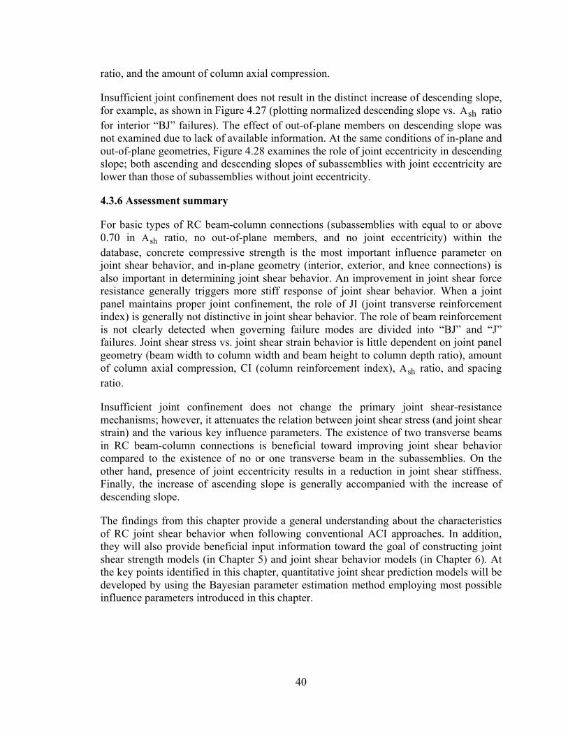
40

ratio, and the amount of column axial compression.

Insufficient joint confinement does not result in the distinct increase of descending slope, for example, as shown in Figure 4.27 (plotting normalized descending slope vs. shA ratio for interior “BJ” failures). The effect of out-of-plane members on descending slope was not examined due to lack of available information. At the same conditions of in-plane and out-of-plane geometries, Figure 4.28 examines the role of joint eccentricity in descending slope; both ascending and descending slopes of subassemblies with joint eccentricity are lower than those of subassemblies without joint eccentricity.

4.3.6 Assessment summary

For basic types of RC beam-column connections (subassemblies with equal to or above 0.70 in shA ratio, no out-of-plane members, and no joint eccentricity) within the database, concrete compressive strength is the most important influence parameter on joint shear behavior, and in-plane geometry (interior, exterior, and knee connections) is also important in determining joint shear behavior. An improvement in joint shear force resistance generally triggers more stiff response of joint shear behavior. When a joint panel maintains proper joint confinement, the role of JI (joint transverse reinforcement index) is generally not distinctive in joint shear behavior. The role of beam reinforcement is not clearly detected when governing failure modes are divided into “BJ” and “J” failures. Joint shear stress vs. joint shear strain behavior is little dependent on joint panel geometry (beam width to column width and beam height to column depth ratio), amount of column axial compression, CI (column reinforcement index), shA ratio, and spacing ratio.

Insufficient joint confinement does not change the primary joint shear-resistance mechanisms; however, it attenuates the relation between joint shear stress (and joint shear strain) and the various key influence parameters. The existence of two transverse beams in RC beam-column connections is beneficial toward improving joint shear behavior compared to the existence of no or one transverse beam in the subassemblies. On the other hand, presence of joint eccentricity results in a reduction in joint shear stiffness. Finally, the increase of ascending slope is generally accompanied with the increase of descending slope.

The findings from this chapter provide a general understanding about the characteristics of RC joint shear behavior when following conventional ACI approaches. In addition, they will also provide beneficial input information toward the goal of constructing joint shear strength models (in Chapter 5) and joint shear behavior models (in Chapter 6). At the key points identified in this chapter, quantitative joint shear prediction models will be developed by using the Bayesian parameter estimation method employing most possible influence parameters introduced in this chapter.

41

point A

point Bpoint C

Story shear, k (1 k = 4.45 kN)

Story displacement, in. (1 in. = 25.4 mm)

(a) Story shear vs. Story displacement

point A

point Bpoint C

Story shear, k (1 k = 4.45 kN)

Joint shear strain (millirad)

(b) Story shear vs. Joint shear strain

Figure 4.1 Comparison of points displaying distinct stiffness changes (test data per Leon, 1990)

42

0

2

4

6

8

10

12

14

16

0 2 4 6 8 10 12 14

Computed joint shear stress (at cracking point)

Expe

rimen

tal j

oint

she

ar s

tres

s (a

t poi

nt A

)

Interior connectionsExterior connectionsKnee connections

Joint panel diagonalcracking: point A

Story shear

Story drift

Figure 4.2 Experimental joint shear stress vs. computed joint shear stress (at point A)

0.0000

0.0002

0.0004

0.0006

0.0008

0.0010

0.0000 0.0002 0.0004 0.0006 0.0008 0.0010

Computed joint shear strain (at cracking point)

Expe

rimen

tal j

oint

she

ar s

trai

n (a

t poi

nt A

)

Interior connectionsExterior connectionsKnee connections

Joint panle diagonalcracking: point A

Joint shear stress

Joint shear strain

Joint shear strain

Figure 4.3 Experimental joint shear strain vs. computed joint shear strain (at point A)

43

0

5

10

15

20

25

30

0 20 40 60 80 100 120

Concrete compressive strength (MPa)

Expe

rimen

tal j

oint

she

ar s

tres

s (M

Pa, a

t poi

nt B

)

Interior joints, J, CC=0.94Interior joints, BJ, CC=0.91Exterior joints, BJ, CC=0.86Knee joints, BJ, CC=0.25

point B

Story shear

Story drift

(a) Joint shear stress vs. Concrete compressive strength

0

5

10

15

20

25

30

0 2 4 6 8 10 12

The square root of concrete compressive strength (MPa0.5)

Expe

rimen

tal j

oint

she

ar s

tres

s (M

Pa, a

t poi

nt B

)

Interior joints, J, CC=0.93Interior joints, BJ, CC=0.91Exterior joints, BJ, CC=0.86Knee joints, BJ, CC=0.24

point B

Story shear

Story drift

(b) Joint shear stress vs. Square root of concrete compressive strength

Figure 4.4 Concrete compressive strength and square root of concrete compressive strength (point B)

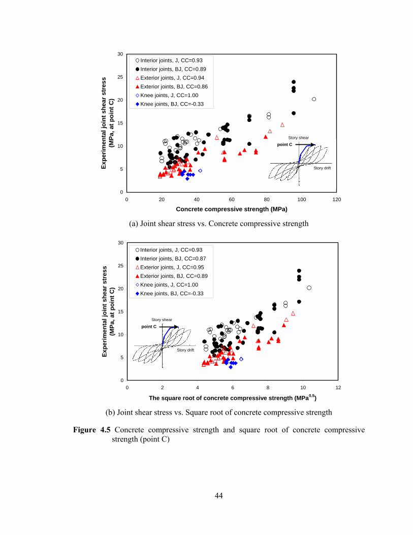
44

0

5

10

15

20

25

30

0 20 40 60 80 100 120

Concrete compressive strength (MPa)

Expe

rimen

tal j

oint

she

ar s

tres

s (M

Pa, a

t poi

nt C

)

Interior joints, J, CC=0.93Interior joints, BJ, CC=0.89Exterior joints, J, CC=0.94Exterior joints, BJ, CC=0.86Knee joints, J, CC=1.00Knee joints, BJ, CC=-0.33

point CStory shear

Story drift

(a) Joint shear stress vs. Concrete compressive strength

0

5

10

15

20

25

30

0 2 4 6 8 10 12

The square root of concrete compressive strength (MPa0.5)

Expe

rimen

tal j

oint

she

ar s

tres

s (M

Pa, a

t poi

nt C

)

Interior joints, J, CC=0.93Interior joints, BJ, CC=0.87Exterior joints, J, CC=0.95Exterior joints, BJ, CC=0.89Knee joints, J, CC=1.00Knee joints, BJ, CC=-0.33

point CStory shear

Story drift

(b) Joint shear stress vs. Square root of concrete compressive strength

Figure 4.5 Concrete compressive strength and square root of concrete compressive strength (point C)

45

0.00

0.01

0.02

0.03

0.04

0.05

0 2 4 6 8 10 12

The square root of concrete compressive strength (MPa0.5)

Expe

rimen

tal j

oint

she

ar s

trai

n (R

ad, a

t poi

nt B

)

Interior joints, J, CC=0.85Interior joints, BJ, CC=0.75Exterior joints, BJ, CC=0.66Knee joints, BJ, CC=0.29

point B

Joint shear stress

Joint shear strain

(a) point B

0.00

0.01

0.02

0.03

0.04

0.05

0 2 4 6 8 10 12

The square root of concrete compressive strength (MPa0.5)

Expe

rimen

tal j

oint

she

ar s

trai

n (R

ad, a

t poi

nt C

)

Interior joints, J, CC=0.61Interior joints, BJ, CC=0.04Exterior joints, J, CC=0.59Exterior joints, BJ, CC=-0.04Knee joints, J, CC=N/AKnee joints, BJ, CC=0.08

point C

Joint shear stress

Joint shear strain

(b) point C

Figure 4.6 Joint shear strain vs. Square root of concrete compressive strength (points B and C)

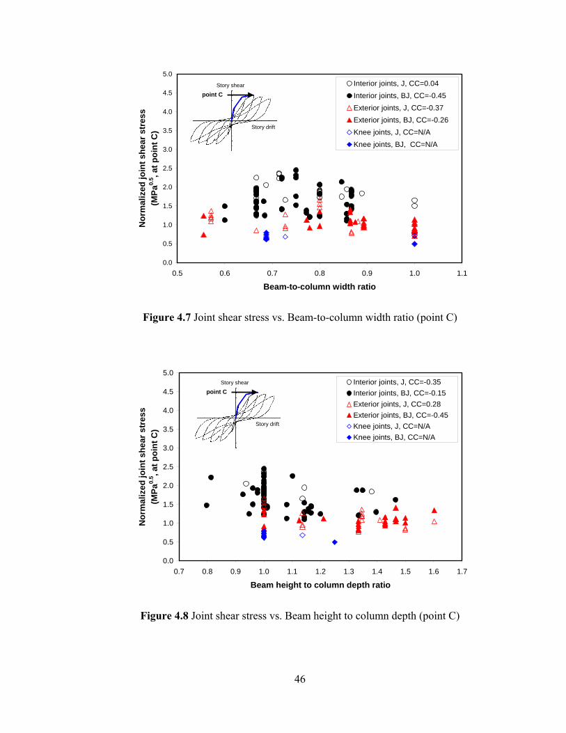
46

0.0

0.5

1.0

1.5

2.0

2.5

3.0

3.5

4.0

4.5

5.0

0.5 0.6 0.7 0.8 0.9 1.0 1.1

Beam-to-column width ratio

Nor

mal

ized

join

t she

ar s

tres

s (M

Pa0.

5 , at p

oint

C)

Interior joints, J, CC=0.04Interior joints, BJ, CC=-0.45Exterior joints, J, CC=-0.37Exterior joints, BJ, CC=-0.26Knee joints, J, CC=N/AKnee joints, BJ, CC=N/A

point CStory shear

Story drift

Figure 4.7 Joint shear stress vs. Beam-to-column width ratio (point C)

0.0

0.5

1.0

1.5

2.0

2.5

3.0

3.5

4.0

4.5

5.0

0.7 0.8 0.9 1.0 1.1 1.2 1.3 1.4 1.5 1.6 1.7

Beam height to column depth ratio

Nor

mal

ized

join

t she

ar s

tres

s (M

Pa0.

5 , at p

oint

C)

Interior joints, J, CC=-0.35Interior joints, BJ, CC=-0.15Exterior joints, J, CC=0.28Exterior joints, BJ, CC=-0.45Knee joints, J, CC=N/AKnee joints, BJ, CC=N/A

point CStory shear

Story drift

Figure 4.8 Joint shear stress vs. Beam height to column depth (point C)

47

0.0

0.5

1.0

1.5

2.0

2.5

3.0

3.5

4.0

4.5

5.0

0.00 0.05 0.10 0.15 0.20 0.25 0.30

JI: Joint transverse reinforcement index

Nor

mal

ized

exp

erim

enta

l joi

nt s

hear

str

ess

(MPa

0.5 , a

t poi

nt C

)

Interior joints, J, CC=-0.04Interior joints, BJ, CC=-0.06Exterior joints, J, CC=0.70Exterior joints, BJ, CC=0.29Knee joints, J, CC=0.46Knee joints, BJ, CC=0.43

point CStory shear

Story drift

(a) Normalized joint shear stress

0.00

0.01

0.02

0.03

0.04

0.05

0.00 0.05 0.10 0.15 0.20 0.25 0.30

JI: Joint transverse reinforcement index

Expe

rimen

tal j

oint

she

ar s

trai

n (R

ad, a

t poi

nt C

)

Interior joints, J, CC=0.13Interior joints, BJ, CC=-0.09Exterior joints, J, CC=0.74Exterior joints, BJ, CC=-0.13Knee joints, J, CC=N/AKnee joints, BJ, CC=N/A

point C

Joint shear stress

Joint shear strain

(b) Joint shear strain

Figure 4.9 Role of joint transverse reinforcement (point C)

48

0.0

0.5

1.0

1.5

2.0

2.5

3.0

3.5

4.0

4.5

5.0

0.0 0.2 0.4 0.6 0.8 1.0 1.2

BI: Beam reinforcement index

Nor

mal

ized

join

t she

ar s

tres

s (M

Pa0.

5 , at p

oint

C)

Interior joints, J, CC=0.36Interior joints, BJ, CC=0.20Exterior joints, J, CC=0.34Exterior joints, BJ, CC=0.20Knee joints, J, CC=N/AKnee joints, BJ, CC=N/A

point CStory shear

Story drift

(a) Normalized joint shear stress

0.00

0.01

0.02

0.03

0.04

0.05

0.0 0.2 0.4 0.6 0.8 1.0 1.2

BI: Beam reinforcement index

Join

t she

ar s

trai

n (R

ad, a

t poi

nt C

)

Interior joints, J, CC=-0.12Interior joints, BJ, CC=0.01Exterior joints, J, CC=0.18Exterior joints, BJ, CC=-0.48Knee joints, J, CC=N/AKnee joints, BJ, CC=N/A

point C

Joint shear stress

Joint shear strain

(b) Joint shear strain

Figure 4.10 Role of beam reinforcement (point C)

49

0.0

0.5

1.0

1.5

2.0

2.5

3.0

3.5

4.0

4.5

5.0

0.0 0.2 0.4 0.6 0.8 1.0 1.2 1.4

CI: Column reinforcement index

Nor

mal

ized

exp

erim

enta

l joi

nt s

hear

str

ess

(MPa

0.5 , a

t poi

nt C

)

Interior joints, J, CC=0.30Interior joints, BJ, CC=-0.29Exterior joints, J, CC=-0.18Exterior joints, BJ, CC=0.04Knee joints, J, CC=0.48Knee joints, BJ, CC=-0.29

point CStory shear

Story drift

(a) Normalized joint shear stress

0.00

0.01

0.02

0.03

0.04

0.05

0.0 0.2 0.4 0.6 0.8 1.0 1.2 1.4

CI: Column reinforcement index

Join

t she

ar s

trai

n (R

ad, a

t poi

nt C

)

Interior joints, J, CC=-0.39Interior joints, BJ, CC=-0.11Exterior joints, J, CC=-0.42Exterior joints, BJ, CC=-0.13Knee joints, J, CC=N/AKnee joints, BJ, CC=N/A

point C

Joint shear stress

Joint shear strain

(b) Joint shear strain

Figure 4.11 Role of column reinforcement (point C)

50

0.0

0.5

1.0

1.5

2.0

2.5

3.0

3.5

4.0

4.5

5.0

0.0 0.1 0.2 0.3 0.4 0.5 0.6 0.7

Column axial stress / Concrete compressive strength

Nor

mal

ized

join

t she

ar s

tres

s (M

Pa0.

5 , at p

oint

C)

Interior joints, J, CC=0.38

Interior joints, BJ, CC=0.27

Exterior joints, J, CC=-0.25

Exterior joints, BJ, CC=-0.15

point CStory shear

Story drift

(a) Normalized joint shear stress

0.000

0.005

0.010

0.015

0.020

0.025

0.030

0.035

0.040

0.045

0.050

0.00 0.05 0.10 0.15 0.20 0.25 0.30 0.35 0.40 0.45 0.50

Column axial stress / Concrete compressive strength

Join

t she

ar s

trai

n (R

ad, a

t poi

nt C

)

Interior joints, J, CC=-0.06

Interior joints, BJ, CC=-0.37

Exterior joints, J, CC=0.46

Exterior joints, BJ, CC=0.08

point C

Joint shear stress

Joint shear strain

(b) Joint shear strain

Figure 4.12 Role of column axial compression (point C)

51

0.0

0.5

1.0

1.5

2.0

2.5

3.0

0 1 2 3 4 5

Bon

d de

man

d le

vel (

MPa

0.5 , a

t poi

nt B

)

Interior joints, BJ, beam reinforcementInterior joints, BJ,column reinforcementInterior joints, J, beam reinforcementInterior joints, J, column reinforcement

Upper limit for column reinforcement

Upper limit for beam reinforcement

point B

Story shear

Story drift

(a) point B

0.0

0.5

1.0

1.5

2.0

2.5

3.0

0 1 2 3 4 5

Bon

d de

man

d le

vel (

MPa

0.5 , a

t poi

nt C

)

Interior joints, BJ, column reinforcementInterior joints, J, beam reinforcementInterior joints, J, column reinforcement

Upper limit for beam reinforcement

Upper limit for column reinforcement

point CStory shear

Story drift

(b) point C

Figure 4.13 Calculated bond demand levels for interior joints (points B and C)

52

0.0

0.5

1.0

1.5

2.0

2.5

3.0

3.5

4.0

4.5

5.0

0.0 0.2 0.4 0.6 0.8 1.0 1.2 1.4 1.6 1.8 2.0

Bond demand level for beam or column reinforcement

Nor

mal

ized

exp

erim

enta

l joi

nt s

hear

str

ess

(MPa

0.5 , a

t poi

nt C

)

Interior joints, J, beam reinforcement, CC=0.65

Interior joints, J, column reinforcement, CC=0.26

Interior joints, BJ, column reinforcement, CC=0.25

Upper limit for column reinforcement Upper limit for beam reinforcement

point CStory shear

Story drift

(a) Normalized joint shear stress

0.000

0.005

0.010

0.015

0.020

0.025

0.030

0.035

0.040

0.045

0.050

0.0 0.2 0.4 0.6 0.8 1.0 1.2 1.4 1.6 1.8 2.0

Bond demand level for beam or column reinforcement

Expe

rimen

tal j

oint

she

ar s

trai

n (R

ad, a

t poi

nt C

)

Interior joints, J, beam reinforcement, CC=-0.76

Interior joints, J, column reinforcement, CC=-0.62

Interior joints, BJ, column reinforcement, CC=-0.30

Upper limit for column reinforcement Upper limit for beam reinforcement

point C

Joint shear stress

Joint shear strain

(b) Joint shear strain

Figure 4.14 Role of bond demand levels of beam and column reinforcement for interior joints (point C)

53

0.00

0.02

0.04

0.06

0.08

0.10

0.12

0.14

0.16

0.0 0.1 0.2 0.3 0.4 0.5

Experimental joint shear stress (at point B ) / Concrete compressive strength

Expe

rimen

tal j

oint

she

ar s

trai

n (p

oint

B) /

B

eam

rein

forc

emen

t ind

ex

Interior joints with 2TB (Equal to or above 0.70 in Ash ratio)Interior joints with 1TB (Equal to or above 0.70 in Ash ratio)Interior joints with 0TB (Equal to or above 0.70 in Ash ratio)

point B

Joint shear stress

Joint shear strain

(a) point B

0.00

0.02

0.04

0.06

0.08

0.10

0.12

0.14

0.16

0.0 0.1 0.2 0.3 0.4 0.5

Experimental joint shear stress (at point C) / Concrete compressive strength

Expe

rimen

tal j

oint

she

ar s

trai

n (a

t poi

nt C

) /

Bea

m re

info

rcem

ent i

ndex

Interior joints with 2 TB (Equal to or above 0.70 in Ash ratio)Interior joints with 1 TB (Equal to or above 0.70 in Ash ratio)Interior joints with 0 TB (Equal to or above 0.70 in Ash ratio)

point C

Joint shear stress

Joint shear strain

(b) point C

Figure 4.15 Joint shear strain to BI vs. Joint shear stress to concrete compressive strength (points B and C)

54

0

5

10

15

20

25

30

0 20 40 60 80 100 120 140

Concrete compressive strength (MPa)

Expe

rimen

tal j

oint

she

ar s

tres

s (M

Pa, a

t poi

nt B

)

Interior J (Without TB and ECC)Interior BJ (Without TB and ECC)Exterior BJ (Without TB and ECC)Knee BJ (Without TB and ECC)

point B

Story shear

Story drift

(a) point B

0

5

10

15

20

25

30

0 20 40 60 80 100 120 140

Concrete compressive strength (MPa)

Expe

rimen

tal j

oint

she

ar s

tres

s (M

Pa, a

t poi

nt C

)

Interior J (Without TB and ECC)Interior BJ (Without TB and ECC)Exterior J (Without TB and ECC)Exterior BJ (Without TB and ECC)Knee J (Without TB and ECC)Knee BJ (Without TB and ECC)

point CStory shear

Story drift

(b) point C

Figure 4.16 Joint shear stress vs. concrete compressive strength (points B and C)

55

0

5

10

15

20

25

30

0 20 40 60 80 100 120 140

Concrete compressive strength (MPa)

Expe

rimen

tal j

oint

she

ar s

tres

s (M

Pa, a

t poi

nt C

)

Interior BJ (Equal to or above 0.70 in Ash ratio)

Interior BJ (below 0.70 in Ash ratio)

point CStory shear

Story drift

(a) Governing failure mode: “BJ”

0

5

10

15

20

25

30

0 20 40 60 80 100 120

Concrete compressive strength (MPa)

Expe

rimen

tal j

oint

she

ar s

tres

s (M

Pa, a

t poi

nt C

)

Interior J (Equal to or above 0.70 in Ash ratio)

Interior J (below 0.70 in Ash ratio)

point CStory shear

Story drift

(b) Governing failure mode: “J”

Figure 4.17 Effect of insufficient joint confinement (Interior joint at point C)

56

0.0

0.5

1.0

1.5

2.0

2.5

3.0

0.00 0.05 0.10 0.15 0.20 0.25 0.30

Joint transverse reinforcement index

Nor

mal

ized

exp

erim

enta

l joi

nt s

hear

str

ess

(poi

nt C

, MPa

0.5 )

Interior J (Equal to or above 0.70 in Ash ratio)Interior J (Below 0.70 in Ash ratio)Exterior J (Equal to or above 0.70 in Ash ratio)Exterior J (Below 0.70 in Ash ratio)Knee J (Equal to or above 0.70 in Ash ratio)Knee J (Below 0.70 in Ash ratio)

point CStory shear

Story drift

(a) Joint shear stress

0.000

0.005

0.010

0.015

0.020

0.025

0.030

0.035

0.040

0.045

0.050

0.00 0.05 0.10 0.15 0.20 0.25 0.30

Joint transverse reinforcement index

Expe

rimen

tal j

oint

she

ar s

trai

n (p

oint

C, R

ad)

Interior J (Equal to or above 0.70 in Ash ratio)Interior J (Below 0.70 in Ash ratio)Exterior J (Equal to or above 0.70 in Ash ratio)Exterior J (Below 0.70 in Ash ratio)Knee J (Below 0.70 in Ash ratio)

point C

Joint shear stress

Joint shear strain

(b) Joint shear strain

Figure 4.18 Role of joint transverse reinforcement (“J” failure, point C, including subassemblies with insufficient joint confinement)

57

0.0

0.5

1.0

1.5

2.0

2.5

3.0

0 0.5 1 1.5 2 2.5 3 3.5 4 4.5

Com

pute

d bo

nd d

eman

d le

vel (

poin

t B, M

Pa0.

5 ) Interior BJ (Equal to or above 0.70 in Ash ratio)Interior BJ (Below 0.70 in Ash ratio)Interior J (Equal to or above 0.70 in Ash ratio)Interior J (Below 0.70 in Ash ratio)

point B

Story shear

Story drift

Upper limit for beam reinforcement

(a) point B

0.0

0.5

1.0

1.5

2.0

2.5

3.0

0 1 2 3

Com

pute

d bo

nd d

eman

d le

vel (

poin

t C, M

Pa0.

5 ) Interior J (Equal to or above 0.70 in Ash ratio)

Interior J (Below 0.70 in Ash ratio)

Upper limit for beam reinforcement

point CStory shear

Story drift

(b) point C

Figure 4.19 Bond demand levels for beam reinforcement (including subassemblies with insufficient confinement)

58

0.0

0.5

1.0

1.5

2.0

2.5

3.0

0.0 0.5 1.0 1.5 2.0

Computed bond demand level for beam reinforcement (point C, MPa0.5)

Nor

mal

ized

exp

erim

enta

l joi

nt s

hear

str

ess

(poi

nt C

, MPa

0.5 )

Interior J (Equal to or above 0.70 in Ash ratio)

Interior J (Below 0.70 in Ash ratio)

point CStory shear

Story drift

Upper limit for beam reinforcement

(a) Normalized joint shear stress

0.00

0.01

0.02

0.03

0.04

0.05

0.0 0.5 1.0 1.5 2.0

Computed bond demand level for beam reinforcement (point C, MPa0.5)

Expe

rimen

tal j

oint

she

ar s

trai

n (p

oint

C, R

ad)

Interior J (Equal to or above 0.70 in Ash ratio)Interior J (Below 0.70 in Ash ratio)

point C

Joint shear stress

Joint shear strain

Upper limit for beam reinforcement

(b) Joint shear strain

Figure 4.20 Role of bond demand levels for beam reinforcement (at point C, including subassemblies with insufficient joint confinement)

59

0.00

0.02

0.04

0.06

0.08

0.10

0.12

0.14

0.16

0.18

0.20

0.00 0.10 0.20 0.30 0.40 0.50

Experimental joint shear stress (point B) / Concrete compressive strength

Expe

rimen

tal j

oint

she

ar s

trai

n (p

oint

B) /

B

eam

rein

forc

emen

t ind

ex

Interior (Equal to or above 0.70 in Ash ratio)Interior (Below 0.70 in Ash ratio)Exterior (Equal to or above 0.70 in Ash ratio)Exterior (Below 0.70 in Ash ratio)Knee (Equal to or above 0.70 in Ash ratio)Knee (Below 0.70 in Ash ratio)

point B

Joint shear stress

Joint shear strain

(a) point B

0.00

0.02

0.04

0.06

0.08

0.10

0.12

0.14

0.16

0.18

0.20

0.00 0.05 0.10 0.15 0.20 0.25 0.30 0.35 0.40 0.45 0.50

Experimental joint shear stress (point C) / Concrete compressive strength

Expe

rimen

tal j

oint

she

ar s

trai

n (p

oint

C) /

B

eam

rein

forc

emen

t ind

ex

Interior (Equal to or above 0.70 in Ash ratio)Interior (Below 0.70 in Ash ratio)Exterior (Equal to or above 0.70 in Ash ratio)Exterior (Below 0.70 in Ash ratio)Knee (Equal to or above 0.70 in Ash ratio)Knee (Below 0.70 in Ash ratio)

point C

Joint shear stress

Joint shear strain

(b) point C

Figure 4.21 Joint shear strain to BI vs. joint shear stress to concrete compressive strength (including subassemblies with insufficient joint confinement)

60

0

5

10

15

20

25

30

0 20 40 60 80 100 120

Concrete compressive strength (MPa)

Expe

rimen

tal j

oint

she

ar s

tres

s (p

oint

B, M

Pa)

Interior BJ with 2TB (Equal to or above 0.7 in Ash ratio)Interior BJ with 1TB (Equal to 0.70 in Ash ratio)Interior BJ with 0 TB (Equal to or above 0.70 in Ash ratio)

point B

Story shear

Story drift

(a) point B

0

5

10

15

20

25

30

0 20 40 60 80 100 120

Concrete compressive strength (MPa)

Expe

rimen

tal j

oint

she

ar s

tres

s (p

oint

C, M

Pa)

Interior BJ with 2TB (Equal to or above 0.70 in Ash ratio)Interior BJ with 1TB (Equal to or above 0.70 in Ash ratio)Interior BJ with 0TB (Equal to or above 0.70 in Ash ratio)

point CStory shear

Story drift

(b) point C

Figure 4.22 Role of transverse beams in joint shear stress at point B and C

61

0.00

0.02

0.04

0.06

0.08

0.10

0.12

0.14

0.16

0.18

0.20

0.0 0.1 0.2 0.3 0.4 0.5

Experimental joint shear stress (at point B ) / Concrete compressive strength

Expe

rimen

tal j

oint

she

ar s

trai

n (p

oint

B) /

B

eam

rein

forc

emen

t ind

ex

Interior joints with 2TB (Equal to or above 0.70 in Ash ratio)Interior joints with 1TB (Equal to or above 0.70 in Ash ratio)Interior joints with 0TB (Equal to or above 0.70 in Ash ratio)

point B

Joint shear stress

Joint shear strain

(a) point B

0.00

0.02

0.04

0.06

0.08

0.10

0.12

0.14

0.16

0.18

0.20

0.0 0.1 0.2 0.3 0.4 0.5

Experimental joint shear stress (at point C) / Concrete compressive strength

Expe

rimen

tal j

oint

she

ar s

trai

n (a

t poi

nt C

) /

Bea

m re

info

rcem

ent i

ndex

Interior joints with 2 TB (Equal to or above 0.70 in Ash ratio)Interior joints with 1 TB (Equal to or above 0.70 in Ash ratio)Interior joints with 0 TB (Equal to or above 0.70 in Ash ratio)

point C

Joint shear stress

Joint shear strain

(b) point C

Figure 4.23 Role of transverse beams in joint shear strain at point B and C

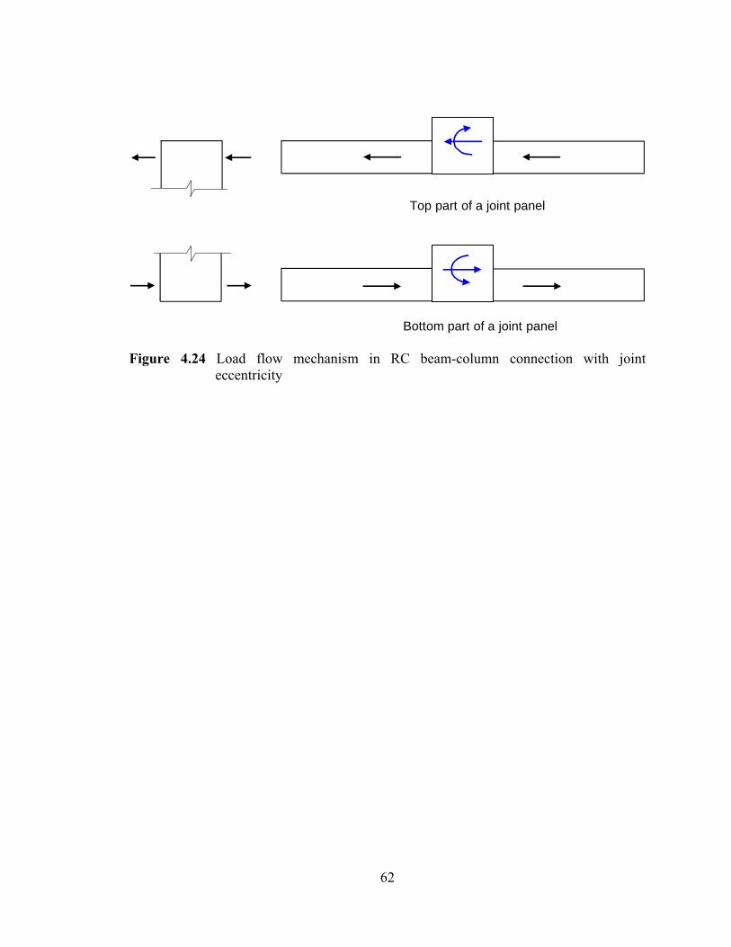
62

Top part of a joint panel

Bottom part of a joint panel

Figure 4.24 Load flow mechanism in RC beam-column connection with joint eccentricity

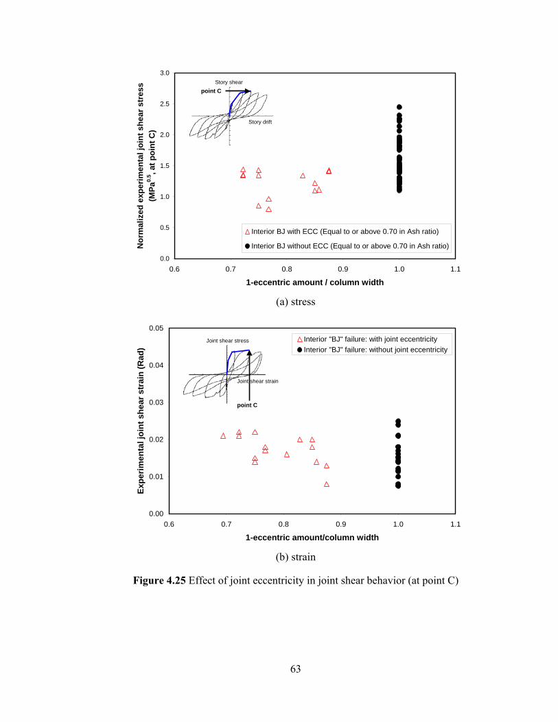
63

0.0

0.5

1.0

1.5

2.0

2.5

3.0

0.6 0.7 0.8 0.9 1.0 1.1

1-eccentric amount / column width

Nor

mal

ized

exp

erim

enta

l joi

nt s

hear

str

ess

(MPa

0.5 , a

t poi

nt C

)

Interior BJ with ECC (Equal to or above 0.70 in Ash ratio)

Interior BJ without ECC (Equal to or above 0.70 in Ash ratio)

point CStory shear

Story drift

(a) stress

0.00

0.01

0.02

0.03

0.04

0.05

0.6 0.7 0.8 0.9 1.0 1.1

1-eccentric amount/column width

Expe

rimen

tal j

oint

she

ar s

trai

n (R

ad)

Interior "BJ" failure: with joint eccentricityInterior "BJ" failure: without joint eccentricity

point C

Joint shear stress

Joint shear strain

(b) strain

Figure 4.25 Effect of joint eccentricity in joint shear behavior (at point C)

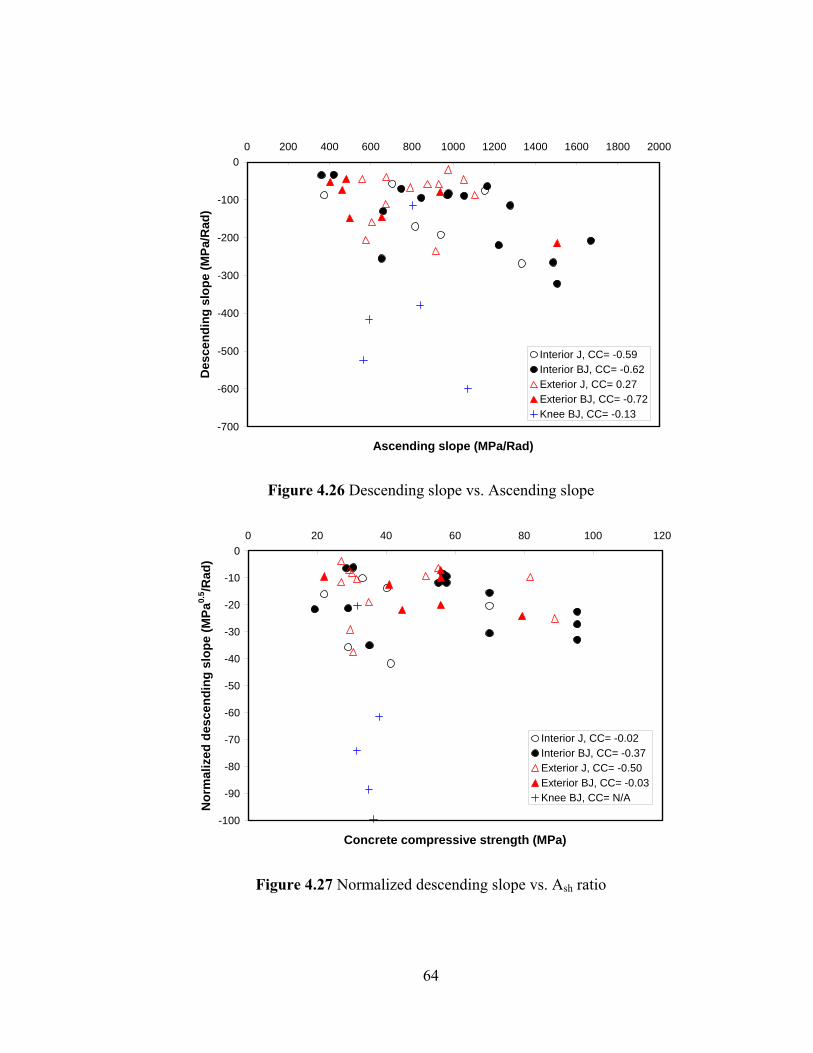
64

-700

-600

-500

-400

-300

-200

-100

00 200 400 600 800 1000 1200 1400 1600 1800 2000

Ascending slope (MPa/Rad)

Des

cend

ing

slop

e (M

Pa/R

ad)

Interior J, CC= -0.59Interior BJ, CC= -0.62Exterior J, CC= 0.27Exterior BJ, CC= -0.72Knee BJ, CC= -0.13

Figure 4.26 Descending slope vs. Ascending slope

-100

-90

-80

-70

-60

-50

-40

-30

-20

-10

00 20 40 60 80 100 120

Concrete compressive strength (MPa)

Nor

mal

ized

des

cend

ing

slop

e (M

Pa0.

5 /Rad

)

Interior J, CC= -0.02Interior BJ, CC= -0.37Exterior J, CC= -0.50Exterior BJ, CC= -0.03Knee BJ, CC= N/A

Figure 4.27 Normalized descending slope vs. Ash ratio

65

-500

-400

-300

-200

-100

00 500 1000 1500 2000

Ascending slope (MPa/Rad)

Des

ccen

ding

slo

pe (M

Pa/R

ad)

Interior BJ, with joint eccentricityInterior BJ, without joint eccentricity

Figure 4.28 Effect of joint eccentricity in descending slope

66

Chapter 5

RC JOINT SHEAR STRENGTH MODEL

A joint shear strength model has been developed using the constructed experimental database, in conjunction with a Bayesian parameter estimation method, for diverse types of RC beam-column connections subjected to seismic lateral loading. In this chapter, the Bayesian parameter estimation method is first introduced. Then, a procedural framework to construct a joint shear strength model is established using the basic dataset (subassemblies with equal to or above 0.70 in shA ratio, no out-of-plane members, and no joint eccentricity). The joint shear strength model has then been continuously updated according to the expansion of the database, and a simple and unified joint shear strength model is finally suggested for diverse types of RC beam-column connections (including those with low shA ratio, out-of-plane members, and joint eccentricity).

Model uncertainty is quantified to evaluate the performance of the developed joint shear strength model by comparison with other deterministic joint shear strength models (of both the “code-based” and the research variety). Joint shear strength for subassemblies with no joint transverse reinforcement is also briefly commented upon. In addition, the effects of “non-standard” conditions (using anchorage plates for longitudinal beam reinforcement, or having fiber-reinforced concrete within a joint panel) on joint shear strength are discussed. Finally, in the last section of this chapter, the ACI 352R-02 model is modified to adjust for shortcomings in the current ACI 352R-02 joint shear strength definition.

5.1 Probabilistic methodology

Recently, probabilistic methods have been applied in an attempt to reduce uncertainty in predicting the capacity of RC members. Probabilistic methods such as Bayesian parameter estimation have most often been applied toward predicting the shear capacity of RC members because shear capacity appears to inherently have more uncertainty (when compared, for instance, with flexural capacity). Gardoni et al. (2002) applied the Bayesian method to construct probabilistic shear capacity models for RC columns, by correcting for the biases in existing deterministic models and quantifying the remaining errors based on collected experimental test results about RC columns. More recently, Sasani (2007) applied the Bayesian method to reduce uncertainty in predicting RC column shear capacity by updating the contribution of parameters that are included in existing deterministic models. Song et al. (2006) also applied the Bayesian method, to suggest probabilistic shear strength models for RC beams with no stirrups; they developed RC beam shear strength models without relying on existing deterministic models. In this research, RC beam-column connection joint shear strength models will be developed (without relying on existing models) to investigate the contribution of various possible influence parameters on RC joint shear strength without being limited by the specific descriptions of existing deterministic models (such as the ACI 352R-02 joint shear strength model).

67

Gardoni et al. (2002) introduced the Bayesian methodology for developing probabilistic shear capacity models of RC columns based on experimental observations. The probabilistic models were constructed by correcting the biases in existing deterministic models and by quantifying the remaining errors. The model predicts the shear capacity ( C ) in the form:

σε+γ+= ),()(c),(C d θΘ xxx (5.1)

where x is the vector of input parameters that were measured during tests, ),( σ= θΘ denotes the set of unknown model parameters that are introduced to fit the model to the test results, )(cd x is the existing deterministic model, ),( θxγ is the bias–correction term, ε is the normal random variable with zero mean and unit variance, and finally σ is the unknown model parameter representing the magnitude of the model error that remains after the bias-correction. Since the true form of the bias-correction term is unknown, the bias-correction term ),( θxγ could be expressed by using a suitable set of p “explanatory” functions, ),(hi x where p,...,1i = , in the form:

∑=

θ=γp

1iii )(h),( xx θ (5.2)

Equation (5.1) also assumes that the variance of the model error is independent of the input parameters x (the so-called “homoskedasticity” assumption). Gardoni et al. (2002) and Song et al. (2006) applied the natural logarithms to satisfy this condition in their applications, that is:

σε+θ+= ∑=

p

1iiid )(h)](cln[)],(Cln[ xxx Θ (5.3)

Bayesian parameter estimation is used in order to find the unknown parameters, ),( σ= θΘ , that make the models in Equations (5.1) or (5.3) best fit the test results. In this

Bayesian approach, the “prior” distributions represent the uncertain parameters based on subjective information, and they are updated to the “posterior” distribution based on objective information such as test results. This well-known updating procedure is described in the form (Box and Tiao, 1992):

)(p)(L)(f ΘΘΘ κ= (5.4)

where )(p Θ is the “prior distribution” that represents the state of knowledge before making observations; )(L Θ is the “likelihood function” that represents objective

information gained from observations; ∫−=κ 1]d)(p)(L[ ΘΘΘ is the “normalizing factor”

(that is, ∫ =κ 0.1d)(p)(L ΘΘΘ ); finally, )(f Θ is the “posterior distribution” that represents the updated knowledge about Θ . If determination of the prior distribution of parameters is difficult, a “non-informative” prior may be applied. Box and Tiao (1992) derived non-

68

informative prior of σ as Equation (5.5); that is:

σ∝σ

1)(p (5.5)

Gardoni et al. (2002) assumed that test results are statistically independent. They then derived a likelihood function based on this assumption; that is:

∏ ⎟⎟⎠

⎞⎜⎜⎝

⎛⎥⎦

⎤⎢⎣

⎡σ

θγ−−ϕ

σ∝

dataFailureiii ),x()x(cC1)(L Θ (5.6)

In Equation (5.6), ( )∏ ∗ represents product of ∗ and )(•ϕ represents the standard normal probability density function (PDF).

The posterior mean vector and covariance vector matrix are usually obtained after updating the distribution of parameters. The posterior mean vector and covariance can be expressed as Equations (5.7) and (5.8), respectively; that is:

∫= ΘΘΘΘ d)(fM (5.7) TT MMd)(f ΘΘΘ ΘΘΘΘ∫ −=∑ (5.8)

Gardoni et al. (2002) employed an importance sampling method to calculate the normalizing factor ( κ ), the posterior mean vector ( ΘM ), and the covariance vector matrix ( Θ∑ ).

For the Bayesian methodology explained above, Gardoni et al. (2002) proposed a systematic procedure to construct a probabilistic capacity model. First, a deterministic capacity model is selected. Then, influence parameters are chosen for explanatory terms in the bias-correction function, based on a general understanding of the physical mechanisms (of structural behavior). The distributions of uncertain parameters Θ are updated by the aforementioned Bayesian parameter estimation method. The explanatory term with iθ having the largest coefficient of variation (c.o.v.) is considered the least informative term of the various influence parameters and is hence removed. This process of updating and subsequent removal is repeated until the posterior mean of σ starts increasing significantly (because σ represents the magnitude of the error after bias-corrections). Finally, the posterior means of s'iθ and σ are substituted into Equations (5.1) or (5.3) to complete the model construction.

Song et al. (2006) applied this Bayesian methodology to construct probabilistic shear strength models for RC beams with no shear reinforcement (i.e. no stirrups). Using Equation (5.3), they developed shear strength models by correcting the biases inherent in six existing deterministic models and then quantifying the remaining scatters. Gardoni et al. (2002) used normalized influencing parameters as explanatory functions; whereas, Song et al. (2006) noted that the natural logarithms of the normalized parameters captured the biases more efficiently. They also suggested a method to construct a

69

model without relying on starting with an existing deterministic model. One of the proposed model forms is then:

σε+θ= ∑=

p

1iii )(h)],(Cln[ xx Θ (5.9)

Due to the lack of a deterministic model in this form, the Bayesian methodology should be used with caution such that the dimension of Equation (5.9) is the same as that of the quantity of interest, even after removing less informative terms. One possible way to assure this is to select a set of explanatory terms that constitutes the same dimension as the quantity of interest and to exclude them from the removal process. One may then add as many possible dimensionless terms as needed, which are subject to the possible removals. Using this method, concrete beam shear strength models that are as accurate as those built upon deterministic models were obtained.

The concrete strut is generally considered as the main joint shear-resistance mechanism in RC beam-column connections. For example, ACI-ASCE Committee 352 accounts for the concrete strut mechanism by using a joint shear strength that is a function of the square root of concrete compressive strength. One major triggered question after a qualitative assessment of various influence parameters on joint shear behavior (in Chapter 4) is about the quantitative contribution and explicit significance of the examined parameters on joint shear behavior, without necessarily being limited by the specific descriptions of existing models. Thus, in this research joint shear models are developed by the Bayesian method employing Equation (5.9).

5.2 RC Joint shear strength model

A procedural framework has been established and is used to construct RC joint shear strength models for the basic dataset. The RC joint shear strength models are then updated by evaluating the effects of insufficient joint confinement, out-of-plane members, and joint eccentricity on joint shear strength. Finally, a simple and unified joint shear strength model, which can be applied to diverse types of RC beam-column connections, will be suggested.

5.2.1 Procedural framework- basic dataset

The examination performed in this section is also reported in Kim et al. (2007). The explanatory terms in Equation (5.9) are first determined to develop joint shear strength models for the basic dataset (subassemblies having equal to or above 0.70 in shA ratio, no out-of-plane members, and no joint eccentricity); most of the examined parameters from back in Section 4.3.1 are selected as explanatory terms. Concrete compressive strength is included to investigate its contribution on overall joint shear strength. To consider a possible reduction in joint shear strength according to in-plane geometry (i.e. for interior, exterior, and knee connections), JP represents a ratio of the number of not-free in-plane surfaces around a joint panel to the total number of in-plane surfaces of the joint panel (4). Thus, JP is 1.0 (4/4) for interior connections, 0.75 (3/4) for exterior connections, and 0.5 (2/4) for knee connections. The ratios of beam height to

70

column depth ( cb hh ) and beam width to column width ( cb bb ) are used to examine whether the shape of the joint panel in the in-plane direction, and the out-of-plane dimensions of in-plane members, respectively, might affect joint shear strength. The joint transverse reinforcement index (JI) and beam reinforcement index (BI) are also included here as explanatory terms. In the recommendations of ACI 352R-02, the cross-sectional area and spacing of joint transverse reinforcement tend to represent the degree of confinement within the joint panel. The shA ratio ( req,shpro,sh AA ) and the spacing ratio ( reqpro ss ) of joint transverse reinforcement are therefore also included to examine whether joint shear strength is at all influenced by the shA ratio and/or the spacing ratio. The database ranges of included parameters are explained in Section 4.3.1.

Based on the observations from 136 experimental test results (using the average of beam and column widths for effective joint shear width), an RC joint shear strength model has been constructed by using the Bayesian method, employing Equation (5.9); the natural logarithms of the eight aforementioned parameters ( '

cf , JP, cb hh , cb bb , JI, BI, req,shpro,sh AA , and reqpro ss ) are used as the explanatory terms ),(hi x .8,...,1i = The

constructed RC joint shear strength model (with the specific exponents noted) can be expressed as Equation (5.10); that is:

( ) ( ) ( ) ( ) 765.0'c

28.1236.00886.0

301.0

cb

0241.0

req,sh

pro,sh0151.0

cb

00513.0

req

proj

fJPBIJI

hh

A

A

bb

s

s04.1)MPa(v ×⎟⎟

⎠

⎞⎜⎜⎝

⎛⎟⎟⎠

⎞⎜⎜⎝

⎛⎟⎟⎠

⎞⎜⎜⎝

⎛⎟⎟⎠

⎞⎜⎜⎝

⎛=

−−

(5.10)

In Equation (5.10), the model uncertainty (i.e. σε ) is not shown for simplicity. The posterior mean of σ is 0.148, which represents model uncertainty after bias-correction.

In Equation (5.10), the spacing ratio ( reqpro ss ) is the least informative of the initial 8 parameters (i.e. the c.o.v. of θ for the spacing ratio is the largest). The remaining 7 parameters are then updated after removing the spacing ratio; the mean of σ is now 0.147. Because the removal of the spacing ratio does not significantly increase the mean of σ , the spacing ratio could be considered as a fairly insignificant parameter on joint shear strength. This process is repeatedly performed until only one parameter remains, which is shown in Table 5.1. Table 5.1 indicates that the mean of σ distinctively increases upon removing JI; thus, joint shear strength for the basic types of RC beam-column connections is more dependent on JI, BI, JP, and '

cf than on cb hh , cb bb , req,shpro,sh AA , and reqpro ss .

RC joint shear strength per Equation (5.11) is developed from the parameters (JI, BI, JP, and 'fc ) surviving the step-wise removal process; that is:

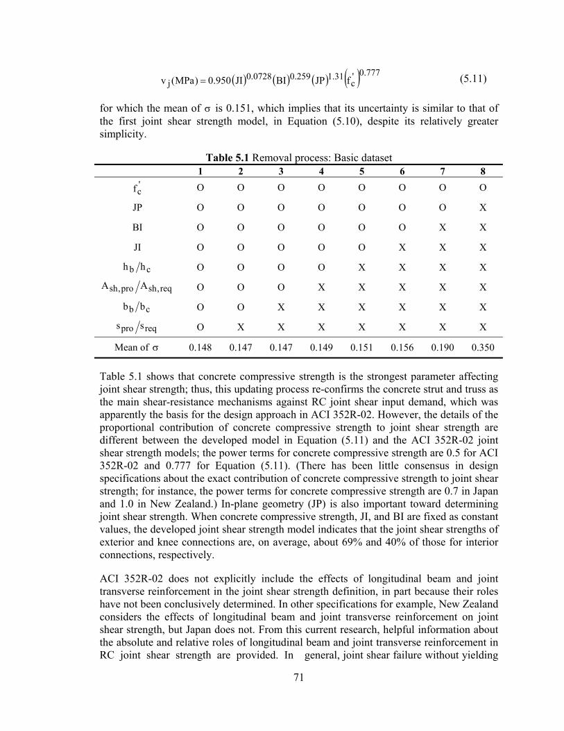
71

( ) ( ) ( ) ( ) 777.0'c

31.1259.00728.0j fJPBIJI950.0)MPa(v = (5.11)

for which the mean of σ is 0.151, which implies that its uncertainty is similar to that of the first joint shear strength model, in Equation (5.10), despite its relatively greater simplicity.

Table 5.1 Removal process: Basic dataset 1 2 3 4 5 6 7 8 'cf O O O O O O O O

JP O O O O O O O X

BI O O O O O O X X

JI O O O O O X X X

cb hh O O O O X X X X

req,shpro,sh AA O O O X X X X X

cb bb O O X X X X X X

reqpro ss O X X X X X X X

Mean of σ 0.148 0.147 0.147 0.149 0.151 0.156 0.190 0.350

Table 5.1 shows that concrete compressive strength is the strongest parameter affecting joint shear strength; thus, this updating process re-confirms the concrete strut and truss as the main shear-resistance mechanisms against RC joint shear input demand, which was apparently the basis for the design approach in ACI 352R-02. However, the details of the proportional contribution of concrete compressive strength to joint shear strength are different between the developed model in Equation (5.11) and the ACI 352R-02 joint shear strength models; the power terms for concrete compressive strength are 0.5 for ACI 352R-02 and 0.777 for Equation (5.11). (There has been little consensus in design specifications about the exact contribution of concrete compressive strength to joint shear strength; for instance, the power terms for concrete compressive strength are 0.7 in Japan and 1.0 in New Zealand.) In-plane geometry (JP) is also important toward determining joint shear strength. When concrete compressive strength, JI, and BI are fixed as constant values, the developed joint shear strength model indicates that the joint shear strengths of exterior and knee connections are, on average, about 69% and 40% of those for interior connections, respectively.

ACI 352R-02 does not explicitly include the effects of longitudinal beam and joint transverse reinforcement in the joint shear strength definition, in part because their roles have not been conclusively determined. In other specifications for example, New Zealand considers the effects of longitudinal beam and joint transverse reinforcement on joint shear strength, but Japan does not. From this current research, helpful information about the absolute and relative roles of longitudinal beam and joint transverse reinforcement in RC joint shear strength are provided. In general, joint shear failure without yielding

72

of beam reinforcement has typically been induced by using a high amount and/or a high yield stress of beam reinforcement, and the joint shear strength of this failure type is typically somewhat higher than that of joint shear failure of a similar connection in conjunction with yielding of beam reinforcement. The formation of plastic hinge(s) between a joint panel and the longitudinal beam(s) can apparently reduce confinement within the joint panel originally provided by the longitudinal beam(s). The beam reinforcement index (BI) roughly represents this phenomenon (in that the beam reinforcement indices for cases without yielding of beam reinforcement were higher than the BI for cases in conjunction with yielding of beam reinforcement). In addition, an increase in BI can improve the confinement within the joint panel, thus, results in an increase in joint shear resistance capacity. Finally, JI appears to be a more appropriate aggregate measure than the shA ratio and/or the spacing ratio to express the effect of beneficial joint confinement provided by joint transverse reinforcement (i.e. the removal of JI triggers a greater increase in the mean of σ than does the removal of the shA ratio or the spacing ratio). However, JI is not a particularly strong influence parameter on joint shear strength within this basic database, in part because the joint panels of this portion of the experimental database were selected considering minimum proper confinement within the joint panel.

Equation (5.11) can be converted into a simple model that could be conveniently used in practical design:

( ) ( ) ( ) 75.0'c

25.007.0bbj fBIJI)MPa(v λα= (5.12)

In Equation (5.12), bα is a parameter for describing in-plane geometry: 1.0 for interior connections, 0.7 for exterior connections, and 0.4 for knee connections; bλ is 1.02, which makes 1.0 in the average of the ratios of Equation (5.11) to Equation (5.12) (and could probably even just conservatively be taken as unity, with little loss in accuracy).

The overall bias and scatter of a deterministic model can also be evaluated by introducing a constant bias-correction term θ (per Song et al. 2006); that is:

σε+θ+= )](cln[)],(Cln[ d xx Θ (5.13)

The overall means of θ and σ can be obtained when a particular suggested joint shear strength model is used as a deterministic model ( )(cd x in Equation (5.13)). A deterministic joint shear strength model is less biased when the posterior mean of θ is more close to zero (with a positive value of θ representing a degree of conservatism), and it has less scatter when the posterior mean of σ is smaller.

When Equation (5.12) is used as a deterministic model ( )(cd x in Equation (5.13)), the overall means of θ and σ are -0.0117 and 0.154, respectively. Therefore, Equation (5.12) is essentially unbiased in determining joint shear strength, which is also confirmed by plotting experimental joint shear stress vs. Equation (5.12) in Figure 5.1. In spite of its greater simplicity, Equation (5.12) also provides a similar level of model uncertainty to

73

that of Equations (5.10) and (5.11), which are completely unbiased.

5.2.2 RC joint shear strength model for reduced dataset

The examination performed in this section is also reported in Kim and LaFave (2007). The constructed experimental database has 182 subassemblies with equal to or above 0.70 in shA ratio (the reduced dataset). For the 13 subassemblies having 1 transverse beam (with/without slab) and no joint eccentricity, the average, maximum, minimum, standard deviation, and coefficient of variation of experimental RC joint shear stress to that from Equation (5.10) are 0.97, 1.28, 0.85, 0.14, and 0.14, respectively. The fourteen subassemblies with joint eccentricity and without out-of-plane members shows that the average, maximum, minimum, standard deviation, and coefficient of variation of experimental joint shear stress to that from Equation (5.10) are 0.88, 1.27, 0.59, 0.20, and 0.22, respectively. Finally, for 16 subassemblies having 2 transverse beams (with/without slab) and no joint eccentricity, the average, maximum, minimum, standard deviation, and coefficient of variation of experimental joint shear stress to that from Equation (5.10) are 1.16, 1.47, 0.92, 0.14, and 0.12, respectively. These statistical results indicate that one transverse beam does not cause any distinct change in joint shear strength. However, two transverse beams provide an improvement in joint shear strength, and, on the other hand, joint eccentricity results in a reduction in joint shear strength (these trends were also visually identified back in Sections 4.3.3 and 4.3.4).

So, then, to extend Equation (5.10) to diverse types of RC beam-column connections, the effects of having 2 transverse beams and/or eccentricity, as noted above, might therefore be considered. Similar to as for JP (the parameter describing in-plane geometry), a change in out-of-plane geometry, which is referred to as TB, is considered by introducing constant values such as 1.0 for subassemblies with 0 or 1 transverse beams and 1.2 for subassemblies with 2 transverse beams. And, as explained back in Section 4.3.4, the degree of joint eccentricity between the beams and the column may be expressed as

cbe1 − .

So, ten parameters are now initially employed to construct joint shear strength models for diverse types of RC beam-column connections. Equation (5.14) is the full joint shear strength model developed by performing the Bayesian method, in the form (with the specific exponents noted) of:

( )

( ) ( ) ( ) ( ) 748.0'c

275.1248.0784.0

c876.0

064.0118.0

cb

029.0

req

pro024.0

req,sh

pro,sh038.0

cb

j

fJPBIbe1TB

JIhh

s

s

A

A

bb

01.1)MPa(v

⎟⎟⎠

⎞⎜⎜⎝

⎛−

×⎟⎟⎠

⎞⎜⎜⎝

⎛⎟⎟⎠

⎞⎜⎜⎝

⎛⎟⎟⎠

⎞⎜⎜⎝

⎛⎟⎟⎠

⎞⎜⎜⎝

⎛=

−−−

(5.14)

In Equation (5.14), the mean of σ is 0.148. The beam-to-column width ratio ( cb bb ) is the least informative of the ten parameters considered. Table 5.2 summarizes the mean of σ according to the removal of the least informative parameter in each step; the mean of

74

σ is distinctively increased after removing joint transverse reinforcement index (JI).

Same as the findings in Table 5.1, Table 5.2 displays that concrete compressive strength ( '

cf ), in-plane geometry (JP), beam reinforcement index (BI), and joint transverse reinforcement (JI) are more important parameters than beam width to column width ( cb bb ), beam height to column depth ( cb hh ), shA ratio ( req,shpro,sh AA ), and spacing ratio ( reqpro ss ) in determining joint shear capacity. According to the inclusion of specimens with out-of-plane members and/or joint eccentricity, out-of-plane geometry (TB) and joint eccentricity ( cbe1 − ) survived after removing insignificant parameters. Because two transverse beams and eccentricity between the beams and the column have already been shown to result in a change of joint shear capacity, it is not surprising that the parameters describing eccentricity ( cbe1 − ) and out-of-plane members (TB) survive after removing parameters that do not cause an increase of σ .

Table 5.2 Removal process: Reduced dataset 1 2 3 4 5 6 7 8 9 10 'cf O O O O O O O O O O

JP O O O O O O O O O X

BI O O O O O O O O X X

cbe1 − O O O O O O O X X X

TB O O O O O O X X X X

JI O O O O O X X X X X

cb hh O O O O X X X X X X

reqpro ss O O O X X X X X X X

req,shpro,sh AA O O X X X X X X X X

cb bb O X X X X X X X X X

Mean of σ 0.148 0.148 0.148 0.148 0.148 0.150 0.155 0.168 0.213 0.331

Joint shear strength per Equation (5.15) is then constructed by updating for the six surviving parameters (JI, TB, cbe1 − , BI, JP, and '

cf ); that is:

( ) ( ) ( ) ( ) ( ) 761.0'c

31.1268.0765.0

c905.0067.0

j fJPBIbe1TBJI00.1)MPa(v ⎟⎟

⎠

⎞⎜⎜⎝

⎛−= (5.15)

The mean of σ is 0.148 for Equation (5.15), which means that the model uncertainty of Equation (5.15) is similar to that of Equation (5.14). Equation (5.15) can be converted into a simple model that could be conveniently used as a practical design expression; that

75

is:

( ) ( ) ( ) 75.0'c

25.007.0rrrrj fBIJI)MPa(v ηλβα= (5.16)

In Equation (5.16), rα is a parameter for describing in-plane geometry: 1.0 for interior connections, 0.7 for exterior connections, and 0.4 for knee connections; rβ is a parameter for describing out-of-plane geometry: 1.0 for subassemblies with 0 or 1 transverse beams and 1.18 for subassemblies with 2 transverse beams; rη ( ( ) 77.0

cbe1 −= ) describes joint eccentricity (equals 1.0 with no joint eccentricity); and rλ is 1.02, which makes 1.0 in the average of the ratios of Equation (5.15) to Equation (5.16). The overall means of θ and σ are –0.0154 and 0.148, respectively for Equation (5.16), and Figure 5.2 plots experimental joint shear stress vs. Equation (5.16). This simple model can predict joint shear strength in an unbiased manner, and it maintains a similar level of model uncertainty to Equations (5.14) and (5.15).

5.2.3 Unified RC joint shear strength model for total database except subassemblies with 0 in Ash ratio

A unified RC joint shear strength model is developed here using the total database (except for the 18 subassemblies with no joint transverse reinforcement). To develop a unified joint shear strength model, a joint shear strength model is first constructed for the subassemblies with below 0.70 in shA ratio (with no joint eccentricity and no out-of-plane members). Within the constructed database, 131 subassemblies had below 0.70 in

shA ratio (with no out-of-plane members and no joint eccentricity). This joint shear strength model is constructed by employing eight explanatory terms, which are the same parameters as in Section 5.2.1. For this database group, the removal process and model uncertainty results are provided in Table 5.3.

Table 5.3 Removal process: Subassemblies with below 0.70 in Ash ratio 1 2 3 4 5 6 7 8 'cf O O O O O O O O

JP O O O O O O O X

BI O O O O O O X X

JI O O O O O X X X

cb hh O O O O X X X X

req,shpro,sh AA O O O X X X X X

reqpro ss O O X X X X X X

cb bb O X X X X X X X

Mean of σ 0.158 0.157 0.157 0.157 0.158 0.174 0.217 0.354

76

Similar to the findings in Table 5.1 (for subassemblies with equal to or above 0.70 in shA ratio), Table 5.3 (subassemblies with below 0.70 in shA ratio) shows that JI, BI, JP,

and 'cf are the surviving significant influence parameters on joint shear strength.

Because insufficient joint confinement does not appear to change the significant influence parameters on joint shear strength, a new joint shear strength model is constructed after removing any limitation on shA ratio. Within the constructed database, 263 subassemblies (136 cases equal to or above 0.70 in shA ratio, and 127 cases below 0.70 in shA ratio) had no out-of-plane members and no joint eccentricity. Equation (5.17) is the constructed joint shear strength model determined by employing eight explanatory terms for these 263 subassemblies; that is:

( ) ( ) ( ) ( ) 785.0'c

30.1283.0103.0

233.0

cb

0713.0

req,sh

pro,sh0171.0

req

pro0213.0

cb

j

fJPBIJI

hh

A

A

s

s

bb

027.1)MPa(v−−

⎟⎟⎠

⎞⎜⎜⎝

⎛⎟⎟⎠

⎞⎜⎜⎝

⎛⎟⎟⎠

⎞⎜⎜⎝

⎛⎟⎟⎠

⎞⎜⎜⎝

⎛=

(5.17)

The mean of σ is 0.153 for Equation (5.17), and Table 5.4 summarizes the model uncertainty according to the removal of explanatory terms. Concrete compressive strength, in-plane geometry, beam reinforcement index, and joint transverse reinforcement index continue to be more important than other parameters in determining joint shear strength. Because there is no distinct difference in the mean of σ and the surviving parameters, a more general joint shear strength model can indeed be developed by removing the limitation on shA ratio.

Table 5.4 Removal process: Total database (except subassemblies with 0 in Ash ratio) 1 2 3 4 5 6 7 8 'cf O O O O O O O O

JP O O O O O O O X

BI O O O O O O X X

JI O O O O O X X X

cb hh O O O O X X X X

req,shpro,sh AA O O O X X X X X

reqpro ss O O X X X X X X

cb bb O X X X X X X X

Mean of σ 0.152 0.152 0.153 0.154 0.155 0.183 0.224 0.370

77

A new RC joint shear strength model is also constructed including only the significant influence parameters on joint shear strength; that is:

( ) ( ) ( ) ( ) 783.0'c

345.1297.0153.0j fJPBIJI17.1)MPa(v = (5.18)

The mean of σ is 0.155 in Equation (5.18). When comparing Equations (5.11) and (5.18), the contributions of concrete compressive strength and in-plane geometry in the developed joint shear strength models are similar. The participation of beam reinforcement is slightly increased after including subassemblies with below 0.70 in shA ratio. The most distinct change between Equations (5.11) and (5.18) is related to the contribution of joint transverse reinforcement to joint shear strength; the power term of JI is changed from 0.07 (in Equation (5.11)) to 0.14 (in Equation (5.18)). Thus, the inclusion of subassemblies with below 0.70 in shA ratio triggers the significance of joint transverse reinforcement as being strengthened in determining joint shear strength.

Based on using Equation (5.17), the effects of out-of-plane members and joint eccentricity have been examined again after removing the database limitation on shA ratio. For the 13 subassemblies with 1 transverse beam (with/without slab and with no joint eccentricity), the average, maximum, minimum, standard deviation, and coefficient of variation of joint shear stress ratio (experimental joint shear stress to Equation (5.17)) are 0.97, 1.28, 0.85, 0.14, and 0.14, respectively. Among these 13 subassemblies, the averages of joint shear stress ratios are 0.95 for 8 cases with no slab and 1.01 for 5 cases with slab. For the 20 subassemblies with 2 transverse beams (with/without slab and with no joint eccentricity), the average, maximum, minimum, standard deviation, and coefficient of variation of joint shear stress ratio are 1.18, 1.49, 0.96, 0.14, and 0.12, respectively. Among these 20 subassemblies, the averages of joint shear stress ratios are 1.16 for 8 cases with no slabs and 1.19 for 12 cases with slabs. The effect of only slab is not considered in the development of RC joint shear strength models because slab results in a slight improvement in RC joint shear strength under the same number of transverse beams. (Most beam-column-slab connections experienced beam flexural failure, thus, the effect of slab on overall behavior (or local behavior) may be more clarified after investigating experimental results with beam flexural failures.) Same as the findings in Section 5.2.2, above results indicate that the presence of 2 transverse beams causes an improvement in RC joint shear strength. Therefore, presence of 2 transverse beams is considered to develop a unified joint shear strength model.

For the 26 subassemblies with joint eccentricity (with/without slab and transverse beams), the average, maximum, minimum, standard deviation, and coefficient of variation of experimental joint shear stress to Equation (5.17) are 0.86, 1.15, 0.62, 0.14, and 0.16, respectively. Same as the findings in Section 5.2.2, joint eccentricity triggers a reduction in RC joint shear strength, thus, it is also further considered next to construct a unified joint shear strength model. Within the constructed database, 323 out of 341 subassemblies are used to construct this unified joint shear strength model (except for subassemblies with 0 in shA ratio).

Before determining finally selected explanatory terms, the effects of following

78

parameters on RC joint shear strength were pre-examined: column axial compression, column reinforcement index, scale effect (describing joint volume ratio to the largest joint volume within the database), column depth ratio (provided-to-recommended column depth ratio for interior connections to check bond condition), and development length ratio (provided-to-recommended length ratio of longitudinal beam reinforcement for exterior and knee connections to check bond condition). The examination results of column axial compression will be explained in Section 6.3. Scale effect and column reinforcement index were not included as the finally selected explanatory terms because both of them were identified as insignificant parameters on RC joint shear strength. Column depth ratio and development length ratio were also not selected as the finally selected explanatory terms because they could not be expressed as one parameter for the development of RC joint shear strength models; in addition, both of them were insignificant parameters on RC joint shear strengths. Finally, ten explanatory terms are determined in the development of RC joint shear strength models for the total database except subassemblies with no joint transverse reinforcement; the selected ten parameters and their ranges are provided in Table 5.5.

Equation (5.19) shows the developed unified joint shear strength model: that is:

( ) ( ) ( ) ( ) ( ) 761.0'c

290.1289.0097.0699.0

c957.0

052.0

req,sh

pro,sh101.0

cb

035.0

cb

010.0

req

proj

fJPBIJIbe1TB

A

A

hh

bb

s

s08.1)MPa(v

⎟⎟⎠

⎞⎜⎜⎝

⎛−

⎟⎟⎠

⎞⎜⎜⎝

⎛⎟⎟⎠

⎞⎜⎜⎝

⎛⎟⎟⎠

⎞⎜⎜⎝

⎛⎟⎟⎠

⎞⎜⎜⎝

⎛=

−−−

(5.19)

Table 5.5 Database ranges of parameters for unified joint shear strength model Parameter Symbol Min. Max. Avg. S.D.

Concrete compressive strength

'cf (Unit: MPa) 19 117 43.77 22.87

In-plane geometry JP (interior=1.0, exterior=0.75, knee=0.5) 0.50 1.00 0.90 0.15

Out-of-plane geometry TB (1.0 for 0 or 1 transverse beam, 1.2 for 2 transverse beams 1.00 1.20 1.01 0.05

Joint eccentricity cbe1 − 0.69 1.00 0.98 0.06

Beam height to column depth cb hh 0.80 2.00 1.11 0.18

Beam width to column width cb bb 0.39 1.00 0.75 0.13 Joint transverse reinforcement

index JI: 'cjyj f)f( ×ρ 0.01 0.26 0.07 0.04

Beam reinforcement index BI: 'cbyb f)f( ×ρ 0.09 1.08 0.37 0.20

Provided-to-recommended cross-sectional area of joint

transverse reinforcement shA ratio: req,shpro,sh AA 0.09 3.54 0.87 0.57

Provided-to-recommended spacing of joint transverse

reinforcement Spacing ratio: reqpro ss 0.36 2.14 0.88 0.41

Min.: Minimum; Max.: Maximum; Avg.: Average; S.D.: Standard Deviation

79

In Equation (5.19), the mean of σ is 0.150, and spacing ratio is the least informative of the ten included parameters. The step-wise removal process is then performed as summarized in Table 5.6. Comparison of Tables 5.2 and 5.6 indicates that the significance of JI is increased after removing the limitation on shA ratio, based on the removal process; JI is removed before eliminating TB and cbe1 − in Table 5.2, however, it is removed after eliminating TB and cbe1 − in Table 5.6. Equation (5.20) is the constructed model after removing the four insignificant parameters on joint shear strength; that is:

( ) ( ) ( ) ( ) ( ) 764.0'c

33.1301.0136.0679.0

c981.0

j fJPBIJIbe1TB21.1)MPa(v ⎟⎟

⎠

⎞⎜⎜⎝

⎛−= (5.20)

In Equation (5.20), the mean of σ is 0.151.

Therefore, a simple and unified joint shear strength model is suggested based on Equation (5.20); that is:

( ) ( ) ( ) 75.0'c

30.015.0ttttj fBIJI)MPa(v ληβα= (5.21)

For Equation (5.21), the overall means of θ and σ are –0.0161 and 0.153, respectively. This means that the simple and unified model (Equation (5.21)) maintains a similar level of reliability as Equations (5.19) and (5.20), and it is almost unbiased in predicting joint shear strength, which is re-confirmed by plotting experimental joint shear stress vs. Equation (5.21), as shown in Figure 5.3. In addition, plot results of joint shear stress ratio (experimental joint shear stress to Equation (5.21)) vs. various explanatory terms (such as concrete compressive strength, in-plane geometry, beam reinforcement index, joint transverse reinforcement index, joint eccentricity, out-of-plane geometry, shA ratio, beam height to column depth, beam width to column width, and spacing ratio) indicate that Equation (5.21) is almost unbiased to the examined parameters within the range of the database (see Figures 5.4 through 5.13).

Finally, then, this simple and unified joint shear strength model (Equation (5.21)) is recommended in determining joint shear strength for diverse types of RC beam-column connections.

80

Table 5.6 Removal process: Total database (except subassemblies 0 in Ash ratio) 1 2 3 4 5 6 7 8 9 10 'cf O O O O O O O O O O

JP O O O O O O O O O X BI O O O O O O O O X X JI O O O O O O O X X X

cbe1 − O O O O O O X X X X TB O O O O O X X X X X

req,shpro,sh AA O O O O X X X X X X

cb hh O O O X X X X X X X cb bb O O X X X X X X X X reqpro ss O X X X X X X X X X

Mean of σ 0.150 0.150 0.150 0.150 0.151 0.156 0.165 0.186 0.231 0.359

5.3 Performance evaluation: Joint shear strength models

ACI 352R-02, ACI 318-05, AIJ 1999, and NZS 3101:1995 all provide their own (deterministic) design joint shear strength models for diverse types of modern RC beam-column connections (maintaining proper confinement within a joint panel). As identified earlier in Sections 3.2 and 3.3, minimum proper confinement within a joint panel is maintained if the shA ratio is equal to or above 0.70. Therefore, the reduced dataset (182 subassemblies) is therefore used in the evaluation of the performance of these code-based deterministic joint shear strength model. Table 5.7 summarizes the overall means of θ and σ for each deterministic model when employing Equation (5.13). Because Equation (5.16) is the simplified model for subassemblies with equal to or above 0.70 in shA ratio, the means of θ and σ for Equation (5.16) are also provided in Table 5.7.

Table 5.7 Posterior means: Code-based deterministic model evaluation Posterior mean Model

θ σ ACI 318-05 0.217 0.308

ACI 352R-02 0.380 0.278 AIJ 1999 0.104 0.198

NZS 3101:1995 0.449 0.428 Equation (5.16) -0.015 0.148

Of these five models, Equation (5.16) has the mean of θ that is the closest to zero (i.e. it is the most unbiased). The means of θ for ACI 318-05, ACI 352R-02, AIJ 1999, and NZS 3101:1995 are positive; these models therefore all determine joint shear strength conservatively. Equation (5.16) also provides the least model uncertainty (the smallest mean of σ ) compared to the other four models. Of the code-based models, AIJ 1999 results in the least scatter in predicting joint shear strength. These examinations indicate that model uncertainty can be distinctively reduced when the power term of concrete compressive strength is around 0.75. Comparing to ACI 352R-02, ACI 318-05

81

has lower conservatism (due to effective joint shear width definition) and model reliability (due to not considering column discontinuity in defining joint shear strength factor). The improved performance of Equation (5.16) can also be visually confirmed by plotting the joint shear stress ratio (experimental joint shear stress to deterministic joint shear strength model values) vs. concrete compressive strength and marking the mean ± one standard deviation, which are shown from Figure 5.14 through Figure 5.17.

In work from other researchers, Russo and Somma (2004) have proposed a joint shear strength model only for exterior connections, and Murakami et al. (2000) proposed a joint shear strength model only for interior connections. These models were not developed for RC beam-column connections with out-of-plane members and/or with joint eccentricity. Table 5.8 summarizes the means of θ and σ for these models, as well as from Equation (5.16).

Table 5.8 Posterior means: Researcher model evaluation Posterior mean Model Experimental subassemblies (No.)

θ σ Murakami et al. Bare interior subassemblies (78) -0.037 0.202 Equation (5.16) Bare interior subassemblies (78) 0.018 0.155

Russo and Somma Bare exterior subassemblies (48) -0.104 0.194 Equation (5.16) Bare exterior subassemblies (48) -0.116 0.122

Because these joint shear strength models did not necessarily focus on safety (i.e. desire conservatism), the means of θ for their models are more close to zero than for code-based models. For only bare interior connections, Equation (5.16) still has improved performance compared to the Murakami et al. model, considering the means of θ and σ . For only exterior connections, the Russo and Somma model is actually less biased than Equation (5.16); however, Equation (5.16) results in less scatter compared to the Russo and Somma model. In spite of the simplicity of Equation (5.16) to apply to diverse types of RC beam-column connections, it still displays improved performance compared to the specialized joint shear strength models proposed by Murakami et al. and Russo and Somma.

5.4 Subassemblies with no joint transverse reinforcement

In a few RC beam-column connection tests, there was no transverse reinforcement within the joint panel. An additional consideration is needed to apply the simple and unified Equation (5.21) to subassemblies with no joint transverse reinforcement because none of the included parameters in Equation (5.21) should be taken as zero. Within the constructed database, 18 subassemblies had no joint transverse reinforcement. For these 18 subassemblies, the experimental joint shear stress to Equation (5.21) ratio can be computed by using a trial value of JI; that is:

( ) ( ) ( ) 75.0'c

30.015.0tttt

exp,j

fBIJI

v

ληβα (5.22)

82

For these subassemblies, the average of Equation (5.22) is 1.0 when the trial JI is equal to 0.0139. This means that using a “virtual” JI of 0.0139 enables Equation (5.21) to predict joint shear strength for subassemblies with no joint transverse reinforcement in an unbiased manner.

The reasonableness of this approach can be examined by evaluating the overall means (of θ and σ ), and it is also visually confirmed based on plot results. For subassemblies with no joint transverse reinforcement, applying 0.0139 for JI in Equation (5.21) provides –0.0126 and 0.151 for overall means of θ and σ , respectively. Almost no bias, and a similar level of model uncertainty, is maintained across subassemblies both with and without joint transverse reinforcement, which is visually confirmed in the plot of Figure 5.18.

5.5 Specific non-standard conditions in RC beam-column connections

The database used in this research only includes test subassemblies with conventional concrete and reinforcement types (a detailed explanation was provided in Section 3.1), and the simple and unified joint shear strength model (Equation (5.21)) was developed using this constructed database. In this section, the effects of “non-standard” specific conditions (using anchorage plates for longitudinal beam reinforcement or fiber-reinforced concrete within a joint panel) on RC joint shear strength are briefly discussed by employing the simple and unified joint shear strength model (Equation (5.21)) to other subassembly groups.

5.5.1 Subassemblies with anchorage plates

An RC joint panel has a complicated reinforcement array due to longitudinal beam, longitudinal column, and joint transverse reinforcement. This is especially true for exterior and knee connections, where longitudinal beam and/or column reinforcement are anchored within the joint panel by 90-degree hooks, which may cause more congestion of the reinforcement array. To relieve this congestion, headed bars or anchorage plates are sometimes used instead of 90-degree hooks for longitudinal beam and/or column reinforcement.

Kaneda et al. (1984), MaConnell and Wallace (1995), Shimonoka (1997), Nakanishi et al. (1998), Shiohara et al. (2002), Choi et al. (2001), Aota et al. (2001), Sato et al. (2002), and Chun et al. (2007) have all conducted experimental subassembly tests to evaluate the performance of RC exterior and/or knee connections with headed bars or anchorage plates. The effect of headed bar (anchorage plate) is examined by employing the simple and unified RC joint shear strength model (Equation (5.21)). Table 5.9 provides available experimental test cases in the evaluation of the effect of headed bar (anchorage plate).

By using 6 exterior cases, the effect of the location of headed bar (anchorage plate) is examined. Because the average of experimental joint shear stress to Equation (5.21) is 0.91 only for exterior connections within the total database, RC joint shear strengths for subassemblies with anchorage plates located within the core of the joint panel are similar to the RC joint shear strength with conventional reinforcement (90-degree hook located

83

within the core of the joint panel). On the other hand, the anchorage plates located beyond the core of the joint panel might increase bond capacity and results in the improvement of RC joint shear strength compared to conventional reinforcement. However, the anchorage plates beyond the core of the joint panel is not recommended because push-out of the anchorage plates in compression can cause the pinching of the overall response of RC beam-column connections.

In Table 5.9, 10 knee experimental test cases display that anchorage plate results in some reduction in RC joint shear strength compared to conventional reinforcement (the average of experimental joint shear stress to Equation (5.21) is 1.15 only for knee connections within the total database). In addition, using anchorage plates in both beam and column reinforcement triggers some additional reduction in RC joint shear strength compared to using anchorage plate in only column reinforcement.

Table 5.9 Experimental test cases with anchorage plate

Beam reinforcement Column reinforcement First

author Name Type )21.5.(Eq,j

exp,jv

v

Plate Location Plate Location Sato RC 3 Ext 1.20 Y Out-core N Sato RC 4 Ext 0.92 Y In-core N

Shiohara RCJ-1 Ext 1.10 Y Out-core N Shiohara RCJ-2 Ext 0.92 Y In-core N Shiohara RCJ-3 Ext 0.90 Y In-core N

Chun JM-2 Ext 1.06 Y In-core N Choi L-3 Knee 1.27 N Y In-core Choi L-4 Knee 0.80 N Y In-core Aota LP15-1 Knee 1.08 N Y In-core Aota LP15-2 Knee 1.00 N Y In-core Aota LP15-3 Knee 1.02 N Y In-core Aota LP18-1 Knee 1.17 N Y In-core Aota LP18-2 Knee 1.09 Y In-core Y In-core Aota LP18-3 Knee 0.87 Y In-core Y In-core Aota LP16-4 Knee 1.29 Y In-core Y In-core Aota LP20-5 Knee 0.88 Y In-core Y In-core

In-core: Anchorage plate is located within the core of the joint panel Out-Core: Anchorage plate is located after passing the core of the joint panel

5.5.2 Fiber-reinforced concrete

Fiber-reinforced concrete (FRC) has been researched to improve the performance of RC structures. In particular, Parra-Montesinos (2005) noted that using FRC results in the improvement of structural performance (such as shear strength, ductility, energy dissipation, and damage tolerance) when RC structures are subjected to reversed cyclic loading. The effect of FRC on joint shear strength is briefly examined here using the simple and unified joint shear strength model (Equation (5.21)).

Henager (1977), Craig et al. (1984), Jindal and Hassan (1984), Gekfen (1986), Jindal and Sharma (1987), Sood and Gupta (1987), Gefken and Ramey (1989), Jiuru et al. (1992), Filiatrault et al. (1994, 1995), Bayasi and Genman (2002), Parra-Montesinos (2005),

84

and Parra-Montesinos et al. (2005) have all researched the performance of FRC in RC beam-column connections. However, most of these experimental tests did not provide enough information (such as actual material strength, geometry, or overall response) to evaluate the performance of FRC. Only two experimental papers are available to examine the effect of FRC by employing Equation (5.21).

First, Craig et al. (1984) tested 10 exterior connections. Half of them (5 subassemblies) had a 1.5% volume fraction of fiber within the joint panel and the others had no fiber within the joint panel. The material property of used fiber is 30 mm-long, 0.5 mm-diameter, and hook-end steel. In addition, the tensile strength of hook-end steel fiber is between 931 MPa and 1379 MPa. Four of ten subassemblies (SP 5, 6, 7, and 8) eventually experienced joint shear failure. Examination results about SP 5, 6, 7, and 8 are summarized in Table 5.10. In Table 5.10, the main difference between SP 5 and SP 6 is the use of FRCC (1.5% by volume) within the joint panel. Using FRCC within the joint panel (SP 6) results in an improvement in joint shear strength, and this tendency is also detected in the comparison of SP 7 and SP 8.

Table 5.10 Effect of FRC (Craig et al., 1984) SP 5 SP 6 SP 7 SP 8

Connection Exterior Exterior Exterior Exterior FRCC No Yes (1.5 %) No Yes (1.5%)

α 0.70 0.70 0.70 0.70 β 1.00 1.00 1.00 1.00 η 1.00 1.00 1.00 1.00 JI 0.07 0.07 0.07 0.07 BI 0.16 0.15 0.32 0.30

'cf 35.03 37.68 34.88 36.32

pex,jv 4.78 5.52 5.36 6.90

21.5.Eq,jv 5.23 5.35 6.36 6.43

21.5.Eq,jpex,j vv 0.91 1.03 0.84 1.07

Parra-Montesinos et al. (2005) tested 2 interior connections with HPFRCC (High-Performance Fiber-Reinforced Cement Composites); the volume fraction of HPFRCC in the joint panel was 1.5%. The HPFRCC used 38 mm-long and 0.038 mm-diameter straight ultra-high molecular weight polyethylene fibers. Parra-Montesinos et al. validated the performance of HPFRCC by comparison with specimen X2 tested previously by Durrani and Wight (1982).

Table 5.11 compares the experimental joint shear stress to Equation (5.21) for both S1 and X2. The difference between specimens S1 and X2 are the use of HPFRCC, JI, and BI. Joint shear stress ratios (experimental joint shear stress to Equation (5.21)) are 0.95 for S1 and 0.92 for X2. As expected, the final governing failure mode of X2 is joint shear failure in conjunction with yielding of beam reinforcement. However, S1 is still governed by beam flexural capacity. This result indicates that using HPFRCC within the joint panel

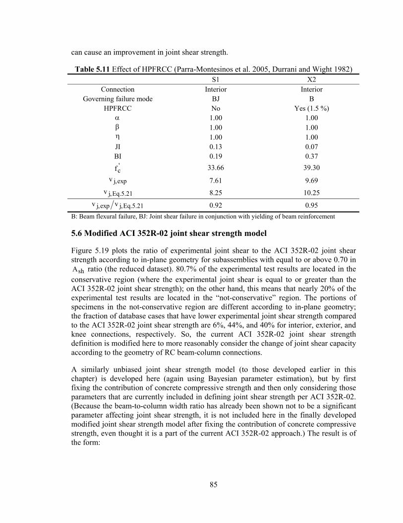
85

can cause an improvement in joint shear strength.

Table 5.11 Effect of HPFRCC (Parra-Montesinos et al. 2005, Durrani and Wight 1982) S1 X2

Connection Interior Interior Governing failure mode BJ B

HPFRCC No Yes (1.5 %) α 1.00 1.00 β 1.00 1.00 η 1.00 1.00 JI 0.13 0.07 BI 0.19 0.37

'cf 33.66 39.30

pex,jv 7.61 9.69

21.5.Eq,jv 8.25 10.25

21.5.Eq,jpex,j vv 0.92 0.95 B: Beam flexural failure, BJ: Joint shear failure in conjunction with yielding of beam reinforcement

5.6 Modified ACI 352R-02 joint shear strength model

Figure 5.19 plots the ratio of experimental joint shear to the ACI 352R-02 joint shear strength according to in-plane geometry for subassemblies with equal to or above 0.70 in

shA ratio (the reduced dataset). 80.7% of the experimental test results are located in the conservative region (where the experimental joint shear is equal to or greater than the ACI 352R-02 joint shear strength); on the other hand, this means that nearly 20% of the experimental test results are located in the “not-conservative” region. The portions of specimens in the not-conservative region are different according to in-plane geometry; the fraction of database cases that have lower experimental joint shear strength compared to the ACI 352R-02 joint shear strength are 6%, 44%, and 40% for interior, exterior, and knee connections, respectively. So, the current ACI 352R-02 joint shear strength definition is modified here to more reasonably consider the change of joint shear capacity according to the geometry of RC beam-column connections.

A similarly unbiased joint shear strength model (to those developed earlier in this chapter) is developed here (again using Bayesian parameter estimation), but by first fixing the contribution of concrete compressive strength and then only considering those parameters that are currently included in defining joint shear strength per ACI 352R-02. (Because the beam-to-column width ratio has already been shown not to be a significant parameter affecting joint shear strength, it is not included here in the finally developed modified joint shear strength model after fixing the contribution of concrete compressive strength, even thought it is a part of the current ACI 352R-02 approach.) The result is of the form:

86

( ) ( ) ( ) 33.1

c

5.0'c

43.103.1j b

e1fJPTB67.1)MPa(v ⎟⎟⎠

⎞⎜⎜⎝

⎛−= (5.23)

In Equation (5.23), the mean of σ is 0.193. This value is larger than the model uncertainty (0.148) for Equation (5.16); however, it is much smaller than the model uncertainty (0.278) for the current ACI 352R-02 model. This means that a more reliable (unbiased and with less scatter) joint shear strength model can even be constructed following the general ACI 352R-02 design equation approach.

Joint shear force can be expressed by multiplying Equation (5.23) by the effective joint shear area; that is, in the form of Equation. (5.24):

( ) ( ) ( ) ccb

33.1

c

5.0'c

43.103.1j h

2bb

be1fJPTB67.1)N(V ⎟

⎠

⎞⎜⎝

⎛ +⎟⎟⎠

⎞⎜⎜⎝

⎛−= (5.24)

Figure 5.20 plots the ratios of experimental joint shear force to model joint shear force (defined by Equation 5.24) vs. in-plane geometry. Because the developed model is unbiased in determining joint shear strength, nearly 50% of the experimental joint shear strengths are necessarily somewhat below Equation (5.24). Two approaches have therefore been introduced in further modifying the ACI 352R-02 joint shear strength model based on Equation (5.24).

5.6.1 First approach in the modification of the ACI 352 model

The developed joint shear strength (Equation (5.24)) is adjusted in order to have only 10% of the cases with lower experimental values than from the developed model (to have similar value to the current statement for interior connections), which can be achieved by applying a factor of 0.75 (representing the mean – 1.295 σ ) to Equation (5.24). This adjusted equation can be expressed in the form of Equation (5.25); that is:

( ) ( ) ( ) ccb

33.1

c5.0

c43.103.1

j h2

bbbe1'fJPTB25.1)N(V ⎟

⎠

⎞⎜⎝

⎛ +⎟⎟⎠

⎞⎜⎜⎝

⎛−= (5.25)

The joint shear strength factor ( γ ) defined by ACI 352R-02 is determined by the in-plane

and out-of-plane connection geometry. Thus, the terms ( ) ( ) 43.103.1 JPTB25.1 above can be considered as the joint shear strength factor defined by Equation (5.25). Because the effective joint shear width defined by ACI 352R-02 is affected by joint eccentricity, the terms ( ) ( ) 2bbbe1 cb

33.1c +− can be considered as the effective joint shear width

defined by Equation (5.25). Table 5.12 shows the modified joint shear strength factors defined by Equation (5.25). Equation (5.25) provides 0.394 and 0.193 for overall means of θ and σ , respectively. Because Equation (5.25) has been adjusted to have 90% conservative cases, the mean of θ is a significant positive value. Equations (5.23) and (5.25) have similar levels of model reliability. Figure 5.21 plots normalized experimental joint shear stress vs. the modified joint shear strength factors defined by Equation

87

(5.25). The portion of normalized experimental joint shear stress cases lower than the modified joint shear strength factors based on Equation (5.25) are 9% for interior connections, 13% for exterior connections, and 0% for knee connections. The modified joint shear strength factors more reasonably consider the change of joint shear capacity according to in-plane geometry, out-of-plane geometry, and joint eccentricity.

Table 5.12 Joint shear strength factors (Equation (5.25)) Joint shear strength factor In-plane geometry No. of transverse

beams ACI 352R-02 Equation (5.25) Interior 0 or 1 1.25 or 1.00 1.25 Exterior 0 or 1 1.00 0.83

Knee 0 or 1 0.67 0.46 Interior 2 1.67 or 1.00 1.50 Exterior 2 1.25 or 1.00 1.00

5.6.2 Second approach in the modification of the ACI 352R-02 model

Both the joint shear strength factors and a strength reduction factor have been suggested to maintain same conservative percentage between the suggested and the current ACI 352R-02 models. When 0.82 is multiplied by Equation (5.24), 79.5% of the experimental results are equal to or above the adjusted joint shear models; this is:

( ) ( ) ( ) ccb

31.1

c

5.0'c

45.103.1j h

2bb

be1fJPTB67.182.0)N(V ⎟

⎠

⎞⎜⎝

⎛ +⎟⎟⎠

⎞⎜⎜⎝

⎛−×= (5.26)

Similar to in the first approach, ( ) ( ) 45.103.1 JPTB67.182.0 × can be considered as the joint shear strength factor defined by Equation (5.26) to maintain the same conservative percentage between Equation (5.26) and the current ACI 352R-02 model. Table 5.13 summarizes the joint shear strength factors defined by Equation (5.26). For Equation (5.26), the overall means of θ and σ are 0.286 and 0.194, respectively; the model uncertainty of Equation (5.26) is similar to that of Equation (5.23). Figure 5.22 plots normalized experimental joint shear stress vs. the joint shear strength factors defined by Equation (5.26). The portion of normalized experimental joint shear stresses lower than the modified joint shear strength factors based on Equation (5.26) are 18% for interior connections, 24% for exterior connections, and 10% for knee connections. These joint shear strength factors defined by Equation (5.26) also reasonably consider the change of joint shear strength according to in-plane geometry, out-of-plane geometry, and joint eccentricity.

In the current ACI 352R-02 design approach, the strength reduction factor ( ACIφ ) is defined as 0.85 for joint shear strength. If this strength reduction factor is applied to the ACI 352R-02 joint shear strength model, then 94.5% of the experimental test results are located in the conservative region. Equation (5.26) can be adjusted to also have 94.5% conservative experimental test results by applying a reduction factor; that is:

88

( ) ( ) ( ) ccb

31.1

c

5.0'c

45.103.1devj h

2bb

be1fJPTB37.1)N(V ⎟

⎠

⎞⎜⎝

⎛ +⎟⎟⎠

⎞⎜⎜⎝

⎛−×φ= (5.27)

where devφ is determined to be 0.89, which is higher than the current ACIφ . The determined reduction factor ( devφ ) shows that this modified ACI 352R-02 model is more reliable than the current ACI 352R-02 joint shear strength model.

Table 5.13 Joint shear strength factors (Equation (5.26)) Joint shear strength factor In-plane geometry No. of transverse

beams ACI 352R-02 Equation (5.26) Interior 0 or 1 1.25 or 1.00 1.37 Exterior 0 or 1 1.00 0.91

Knee 0 or 1 0.67 0.51 Interior 2 1.67 or 1.00 1.65 Exterior 2 1.25 or 1.00 1.10

In summary, two modified ACI 352R-02 models are suggested to consider the changes of RC joint shear strength according to in-plane geometry, out-of-plane geometry, and joint eccentricity more reasonably. In the first approach, joint shear strength factors are adjusted to have the similar statement for interior connections. In the second approach, both joint shear strength factors and a strength reduction factor are adjusted to have the same conservative percentage between the suggested and the current ACI 352R-02 models.

89

0

5

10

15

20

25

30

0 5 10 15 20 25 30

Joint shear model (Equation (5.12), MPa)

Expe

rimen

tal j

oint

she

ar s

tres

s (M

Pa)

Figure 5.1 Experimental joint shear stress vs. Joint shear stress (Equation 5.12)

0

5

10

15

20

25

30

0 5 10 15 20 25 30

Joint shear model (Equation (5.16), MPa)

Expe

rimen

tal j

oint

she

ar s

tres

s (M

Pa)

Figure 5.2 Experimental joint shear stress vs. Joint shear stress defined by Equation (5.16)

90

0

5

10

15

20

25

30

0 5 10 15 20 25 30

Joint shear stress defined by Equation (5.21) (MPa)

Expe

rimen

tal j

oint

she

ar s

tres

s (M

Pa)

Figure 5.3 Experimental joint shear stress vs. Joint shear stress defined by Equation

(5.21)

0.0

0.2

0.4

0.6

0.8

1.0

1.2

1.4

1.6

1.8

2.0

0 20 40 60 80 100 120 140

Concrete compressive strength (MPa)

Join

t she

ar (E

xper

imen

t) /

Join

t she

ar (E

quat

ion

5.21

)

Figure 5.4 Joint shear ratio (Experiment/Equation 5.21) vs. fc’

91

0.0

0.2

0.4

0.6

0.8

1.0

1.2

1.4

1.6

1.8

2.0

0.4 0.5 0.6 0.7 0.8 0.9 1.0 1.1

In-plane geometry (JP)

Join

t she

ar (E

xper

imen

t) /

Join

t she

ar (E

quat

ion

5.21

)

Figure 5.5 Joint shear ratio (Experiment/Equation 5.21) vs. JP

0.0

0.2

0.4

0.6

0.8

1.0

1.2

1.4

1.6

1.8

2.0

0.0 0.2 0.4 0.6 0.8 1.0 1.2

Beam reinforcement index (BI)

Join

t she

ar (E

xper

imen

t) /

Join

t she

ar (E

quat

ion

5.21

)

Figure 5.6 Joint shear ratio (Experiment/Equation 5.21) vs. BI

92

0.0

0.2

0.4

0.6

0.8

1.0

1.2

1.4

1.6

1.8

2.0

0.00 0.05 0.10 0.15 0.20 0.25 0.30Joint transverse reinforcement index (JI)

Join

t she

ar (E

xper

imen

t) /

Join

t she

ar (E

quat

ion

5.21

)

Figure 5.7 Joint shear ratio (Experiment/Equation 5.21) vs. JI

0.0

0.2

0.4

0.6

0.8

1.0

1.2

1.4

1.6

1.8

2.0

0.60 0.65 0.70 0.75 0.80 0.85 0.90 0.95 1.00 1.05 1.10

Joint eccentricity (1-e/bc)

Join

t she

ar (E

xper

imen

t) /

Join

t she

ar (E

quat

ion

5.21

)

Figure 5.8 Joint shear ratio (Experiment/Equation 5.21) vs. 1-e/bc

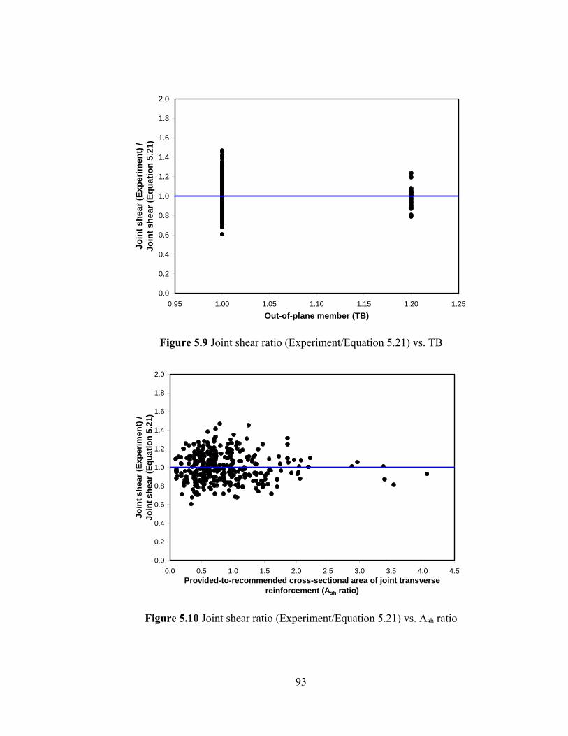
93

0.0

0.2

0.4

0.6

0.8

1.0

1.2

1.4

1.6

1.8

2.0

0.95 1.00 1.05 1.10 1.15 1.20 1.25Out-of-plane member (TB)

Join

t she

ar (E

xper

imen

t) /

Join

t she

ar (E

quat

ion

5.21

)

Figure 5.9 Joint shear ratio (Experiment/Equation 5.21) vs. TB

0.0

0.2

0.4

0.6

0.8

1.0

1.2

1.4

1.6

1.8

2.0

0.0 0.5 1.0 1.5 2.0 2.5 3.0 3.5 4.0 4.5Provided-to-recommended cross-sectional area of joint transverse

reinforcement (Ash ratio)

Join

t she

ar (E

xper

imen

t) /

Join

t she

ar (E

quat

ion

5.21

)

Figure 5.10 Joint shear ratio (Experiment/Equation 5.21) vs. Ash ratio

94

0.0

0.2

0.4

0.6

0.8

1.0

1.2

1.4

1.6

1.8

2.0

0.5 0.7 0.9 1.1 1.3 1.5 1.7 1.9 2.1Beam height to column depth (hb/hc)

Join

t she

ar (E

xper

imen

t) /

Join

t she

ar (E

quat

ion

5.21

)

Figure 5.11 Joint shear ratio (Experiment/Equation 5.21) vs. hb / hc

0.0

0.2

0.4

0.6

0.8

1.0

1.2

1.4

1.6

1.8

2.0

0.3 0.4 0.5 0.6 0.7 0.8 0.9 1.0 1.1Beam width to column width (bb/bc)

Join

t she

ar (E

xper

imen

t) /

Join

t she

ar (E

quat

ion

5.21

)

Figure 5.12 Joint shear ratio (Experiment/Equation 5.21) vs. bb / bc

95

0.0

0.2

0.4

0.6

0.8

1.0

1.2

1.4

1.6

1.8

2.0

0.0 0.5 1.0 1.5 2.0 2.5 3.0Provided-to-recommended spacing of joint transverse reinforcement

(spacing ratio)

Join

t she

ar (E

xper

imen

t) /

Join

t she

ar (E

quat

ion

5.21

)

Figure 5.13 Joint shear ratio (Experiment/Equation 5.21) vs. Spacing ratio

0.0

0.5

1.0

1.5

2.0

2.5

3.0

0 20 40 60 80 100 120

Concrete compressive strength (MPa)

Join

t she

ar s

tres

s ra

tio

Experiemtal joint shear stress / ACI 352R-02

Experimental joint shear stress / Simplified model (for proper joint confinement)

..1 DSMean ±

..1 DSMean ±

For ACI 352R-02Mean + 1 S.D. = 1.63Mean - 1 S.D. = 1.07

For Simplified modelMean + 1 S.D. = 1.15Mean - 1 S.D. = 0.85

Figure 5.14 Comparison of ACI 352R-02 and Equation 5.16

96

0.0

0.5

1.0

1.5

2.0

2.5

3.0

0 20 40 60 80 100 120

Concrete compressive strength (MPa)

Join

t she

ar s

tres

s ra

tio

Experimental joint shear stress / ACI 318-05Experimental joint shear stress / Simplified model (for proper joint confinement)

..1 DSMean ±

..1 DSMean ±

For ACI 318-05Mean + 1 S.D. = 1.53Mean - 1 S.D. = 0.91

For Simplified modelMean + 1 S.D. = 1.15Mean - 1 S.D. = 0.85

Figure 5.15 Comparison of ACI 318-05 and Equation 5.16

0.0

0.5

1.0

1.5

2.0

2.5

3.0

0 20 40 60 80 100 120Concrete compressive strength (MPa)

Join

t she

ar s

tress

ratio

Experimental joint shear stress / AIJ 1999

Experimental joint shear stress / Simplified model (for proper joint confinement)

For Simplified modelMean + 1 S.D. = 1.15Mean - 1 S.D. = 0.85

For AIJ 1999Mean + 1 S.D. = 1.29Mean - 1 S.D. = 0.90

..1 DSMean ±

..1 DSMean ±

Figure 5.16 Comparison of AIJ 1999 and Equation 5.16

97

0.0

0.5

1.0

1.5

2.0

2.5

3.0

0 20 40 60 80 100 120

Concrete compressive strength (MPa)

Join

t she

ar s

tres

s ra

tio

Experimental joint shear stress / NZS 3101Experimental joint shear stress / Simplified model (for proper joint confinement)

..1 DSMean ±

..1 DSMean ±

For Simplified modelMean + 1 S.D. = 1.15Mean - 1 S.D. = 0.85

For NZS 3101: 1995Mean + 1 S.D. = 1.92Mean - 1 S.D. = 1.07

Figure 5.17 Comparison of NZS 3101:1995 and Equation 5.16

0.0

0.5

1.0

1.5

2.0

0.00 0.05 0.10 0.15 0.20 0.25 0.30

JI: Joint transverse reinforcement index

Expe

rimen

t joi

nt s

hear

str

ess

/ Eq

uatio

n (5

.21)

Subassemblies with joint transverse reinforcementSubassemblies without joint transverse reinforcement

.D.S0.1Meam +

.D.S0.1Meam −

Figure 5.18 Uncertainty of Equation (5.21) for the entire range of JI

98

0.0

0.5

1.0

1.5

2.0

2.5

3.0

3.5

4.0

0.40 0.45 0.50 0.55 0.60 0.65 0.70 0.75 0.80 0.85 0.90 0.95 1.00 1.05 1.10

In-plane geometry

Join

t she

ar ra

tio

Joint shear (experiment) / Joint shear (ACI 352R-02)

InteriorExteriorKnee

Knee jointsExterior joints Interior joints

80% cases are equal to or above 1.0

20% cases are below 1.0

Figure 5.19 Current ACI 352R-02 joint shear strength according to in-plane geometry

0.0

0.5

1.0

1.5

2.0

2.5

3.0

0.4 0.5 0.6 0.7 0.8 0.9 1.0 1.1

JP: In-plane geometry

V j (E

xper

imen

t) / V

j (Eq

uatio

n (5

.24)

)

Mean = 1.0

Reduction=0.75Mean - 1 S.D.

Mean - 2 S.D.

Knee joints Exterior joints Interior joints

Figure 5.20 Joint shear model (Equation 5.24) vs. in-plane geometry

99

0.0

0.5

1.0

1.5

2.0

2.5

3.0

3.5

4.0

0.3 0.4 0.5 0.6 0.7 0.8 0.9 1.0 1.1 1.2 1.3 1.4 1.5 1.6 1.7

Joint shear strength factor using Equation (5.25) (MPa0.5)

Nor

mal

ized

exp

erim

enta

l joi

nt s

hear

str

ess

(MPa

0.5 )

Interior joints (with/without out-of-plane members and/or eccentricity)Exterior joints (with/without out-of-plane members and/or eccentricity)Knee joints (without out-of-plane members and/or eccentricity)

Modified ACI Limitation

Experimental shear > Modified ACI 352 model

Experimental shear < Modified ACI 352 model

Figure 5.21 Modified ACI 352R-02 joint shear strength factor (First approach)

0.0

0.5

1.0

1.5

2.0

2.5

3.0

3.5

4.0

0.3 0.4 0.5 0.6 0.7 0.8 0.9 1.0 1.1 1.2 1.3 1.4 1.5 1.6 1.7 1.8

Joint shear strength factor using Equation (5.26) (MPa0.5)

Nor

mal

ized

exp

erim

enta

l joi

nt s

hear

str

ess

(MPa

0.5 )

Interior joints (with/without out-of-plane members and/or eccentricity)Exterior joints (with/without out-of-plane members and/or eccentricity)Knee joints (without out-of-plane members and/or eccentricity)

Modified ACI Limitation

Experimental shear > Modified ACI 352 model

Experimental shear < Modified ACI 352 model

Figure 5.22 Modified ACI 352R-02 joint shear strength factor (Second approach)

100

Chapter 6

RC JOINT SHEAR BEHAVIOR MODEL

An RC beam-column connection subassembly consists of beam(s), a column, and a joint panel. Appropriate analytical models for these components are required to evaluate the seismic response of RC beam-column connection subassemblies (or even of entire RC frames). Using the finite element method is generally not recommended for analyzing RC moment resisting frame (MRF) structures due to issues of time and cost efficiency. In the modeling of RC beam-column connection subassembly or RC moment resisting frame structures, elastic behaviors of beam and column members are typically described as line elements, with the inelastic behaviors of these members represented by (rotational or displacement) spring elements. Joint shear behavior should also be considered in order to properly predict the response of RC beam-column connections more accurately; it may be described as a combination of rotational springs (Shin and LaFave 2004).

At maximum response, a simple and unified joint shear deformation model is suggested below by following the general procedure used above for constructing the simple and unified joint shear strength model. Then, at the other key points of behavior (related to cracking, reinforcement yielding, and descending strength) joint shear behavior models have also been constructed by using the Bayesian parameter estimation method and by adjusting the simple and unified joint shear strength and deformation models (from maximum response). At the final stage, then, a simple and unified joint shear behavior model (RC joint shear stress vs. joint shear strain) is suggested (Table 6.18). For subassemblies with no joint transverse reinforcement, application of the simple and unified model is discussed. The performance of the simple and unified joint shear behavior model is then evaluated by comparison with the FEMA 356 model, the Teraoka and Fujii model, the Parra-Montesinos and Wight model, and the MCFT. In the last section of this chapter, the Parra-Montesinos and Wight model has been modified by updating a key relation in their original method.

6.1 Joint shear deformation model: maximum response (point C)

Overall frame or subassembly story drift is determined by the deflections of beam and column members and the deformation of the joint panel in RC beam-column connections. When the overall response of RC beam-column connections is governed by joint shear, the contribution of the joint panel to overall story deflection increases. This means that joint shear deformation can have a significant impact on overall story drift and that ductile overall response cannot necessarily be guaranteed. Therefore, a joint shear deformation model, as well as the joint shear strength model, may be required to fully understand and maintain reasonable and ductile responses in RC beam-column connections. In spite of the importance of joint shear deformation, there have been few suggestions in the literature about joint shear deformation modeling (compared to a fair number of joint shear strength models).

In this section, an RC joint shear deformation model (at maximum response) will be constructed and updated following the same procedures established back in

101

Section 5.2. Then, a simple and unified joint shear deformation model is suggested for diverse types of RC beam-column connections.

6.1.1 Joint shear deformation model: Basic dataset and reduced dataset

A joint shear deformation model has been first constructed using the basic dataset (subassemblies with equal to or above 0.7 in shA ratio, no out-of-plane members, and no joint eccentricity). As shown in Section 4.3, at point C experimental joint shear strains for “BJ” failures did not show any clear tendency to examined parameters due to the disturbance resulted from the formation of plastic hinges. Because beam reinforcement index (BI) is the best parameter to discern “BJ” and “J” failures, experimental joint shear strain is normalized by beam reinforcement index to remove the effect due to different governing failure mode sequences. Normalized joint shear deformation (joint shear strain to BI) model is here developed by the Bayesian parameter estimation method. Bayesian parameter estimation method should have the same dimension between interest ( C ) and bias correction terms ( ),( θxγ ); the suggested joint shear strength model divided by concrete compressive strength is included as an explanatory term to improve model reliability.

Figure 6.1 plots BIexpγ vs. 'f)10.5(v cj ( )10.5(v j : the developed model for the basic dataset) and shows that BIexpγ is inversely proportional to 'f)10.5(v cj , which is the same finding in Section 4.3.1.6. At the same condition of the experimental joint shear strain normalized by BI, the experimental joint shear stress normalized by concrete compressive strength is decreased in the sequence of interior, exterior, and knee joints. Based on Figure 6.1, a parameter describing in-plane geometry is introduced, which is referred to as JPR. In Figure 6.1, 'f)10.5(v cj could be normalized by JPR to remove the effect by in-plane geometry. The values for JPR for interior, exterior, and knee connections were determined by trial and error to have the strongest relation between experimental joint shear strain normalized by BI and 'f)10.5(v cj normalized by JPR. When JPR is 1.0 for interior, 0.588 for exterior, and 0.323 for knee joints, respectively, the strongest relation can be found in the plot of BIexpγ vs. JPR1'f)10.5(v cj × (Figure 6.2). The reasonableness of the determined values for JPR will be confirmed by removal process in the development of normalized joint shear deformation model. Beam width to column width, beam height to column depth, joint transverse reinforcement index, shA ratio, and spacing ratio are also included as possible explanatory terms in order to develop a normalized joint shear deformation model ( BIγ ).

The normalized joint shear deformation model at point C (for BIγ ) is constructed by the Bayesian method employing the 7 explanatory terms, and it is re-expressed as Equation (6.1); that is:

102

( ) ( ) 08.295.1

'c

10.5.Eq,j164.0

316.0

cb

202.0

req,sh

pro,sh296.0

cb

0409.0

req

pro

JPRf

vJI

hh

A

A

bb

s

sBI00469.0)Rad(

−

−−

⎟⎟

⎠

⎞

⎜⎜

⎝

⎛

×⎟⎟⎠

⎞⎜⎜⎝

⎛⎟⎟⎠

⎞⎜⎜⎝

⎛⎟⎟⎠

⎞⎜⎜⎝

⎛⎟⎟⎠

⎞⎜⎜⎝

⎛=γ

(6.1)

In Equation (6.1), the mean of σ is 0.343; the model uncertainty for joint shear deformation is distinctively greater compared to that (0.148 for σ ) for joint shear strength. Table 6.1 summarizes model uncertainty according to the procedure of removing explanatory terms, one by one. In developing the normalized joint shear deformation model ( BIγ ), JPR, 'f)10.5(v cj , and JI are more important than cb bb , cb hh ,

req,shpro,sh AA , and reqpro ss . In addition, this removal process also confirms that the determined values for JPR are reasonable to describe the effect of in-plane geometry on normalized joint shear strain because JPR remains as a surviving parameter.

Table 6.1 Removal process: Basic dataset (strain at point C) 1 2 3 4 5 6 7

JPR O O O O O O O 'f)10.5(v cj O O O O O O X

JI O O O O O X X

cb hh O O O O X X X

req,shpro,sh AA O O O X X X X

cb bb O O X X X X X

reqpro ss O X X X X X X

Mean of σ 0.342 0.336 0.337 0.336 0.332 0.365 0.614

The joint shear deformation model at point C can be expressed as Equation (6.2) after removing the insignificant influence parameters; that is:

( ) ( ) 18.201.2

'c

11.5.eq,j142.0 JPRf

vJIBI00401.0)Rad(

−

⎟⎟

⎠

⎞

⎜⎜

⎝

⎛=γ (6.2)

There is no change in model uncertainty when Equation (5.11) (the developed model after removing insignificant influence parameters for the basic dataset) is used instead of Equation (5.10) for Equation (6.2). Equation (6.2) yields 0.332 for the mean of σ (a similar level of model uncertainty to Equation (6.1)) and it determines joint shear deformation in an unbiased manner, which is shown in Figure 6.3. The surviving parameters in joint shear strength (Equation (5.11)) and joint shear deformation (Equation (6.2)) are similar; RC joint shear capacity (strength and deformation) is mainly dependent on joint transverse reinforcement, beam reinforcement, in-plane geometry, and concrete

103

compressive strength for the basic dataset.

The effects of out-of-plane members and joint eccentricity on joint shear deformation are examined using Equation (6.1). For the 8 subassemblies with 2 transverse beams (and no joint eccentricity), the average, maximum, minimum, standard deviation, and coefficient of variation of experimental joint shear strain to Equation (6.1) are 1.16, 1.63, 0.47, 0.40, and 0.35, respectively. For the 16 subassemblies with joint eccentricity (and no out-of-plane members), the average, maximum, minimum, standard deviation, and coefficient of variation of experimental joint shear strain to Equation (6.1) are 1.57, 1.97, 0.48, 0.43, and 0.27, respectively. (The effect of one transverse beam on joint shear deformation is not examined due to a lack of experimental information.) The presence of two transverse beams results in an increase in joint shear deformation as well as joint shear strength. On the other hand, joint eccentricity triggers an increase in joint shear deformation along with a decrease in joint shear strength. (These findings were visually shown back in Chapter 4.)

For diverse types of RC beam-column connections with equal to or above 0.70 in shA ratio, a normalized joint shear deformation model may then be constructed using nine explanatory terms. Among the nine explanatory terms, parameters describing out-of-plane geometry and joint eccentricity are included. The degree of joint eccentricity is expressed as cbe1 − ; for out-of-plane geometry (TB), 1.0 is used for subassemblies with one or no transverse beams, and 1.2 for subassemblies with two transverse beams. The constructed joint shear deformation model at point C can be expressed as Equation (6.3); that is:

( ) ( ) ( ) 22.288.1

'c

14.5.eq,j161.084.1814.0

c

935.0

cb

259.0

req,sh

pro,sh241.0

cb

0209.0

req

pro

JPRf

vJITB

be1

bb

A

A

hh

s

sBI00718.0)Rad(

−−

−−

⎟⎟

⎠

⎞

⎜⎜

⎝

⎛⎟⎟⎠

⎞⎜⎜⎝

⎛−

×⎟⎟⎠

⎞⎜⎜⎝

⎛⎟⎟⎠

⎞⎜⎜⎝

⎛⎟⎟⎠

⎞⎜⎜⎝

⎛⎟⎟⎠

⎞⎜⎜⎝

⎛=γ

(6.3)

where the mean of σ is 0.343. Table 6.2 shows the removal process of explanatory terms, and it indicates that model uncertainty is distinctively increased after eliminating cbe1 − .

Equation (6.4) is then constructed joint shear deformation model at point C after removing insignificant parameters; that is:

( ) ( ) ( ) 24.201.2

'c

15.5.eq,j130.076.1751.0

cJPR

f

vJITB

be1BI00405.0)Rad(

−−

⎟⎟

⎠

⎞

⎜⎜

⎝

⎛⎟⎟⎠

⎞⎜⎜⎝

⎛−=γ (6.4)

In Equation (6.4), the mean of σ is not changed when using Equation (5.15) (the developed joint shear strength model after removing insignificant influence parameters for the reduced dataset) instead of Equation (5.14). For Equation (6.4), the mean of σ is

104

0.351, which is a little higher than the mean of σ (0.343) for Equation (6.3).

Table 6.2 Removal process: Reduced dataset (strain at point C) 1 2 3 4 5 6 7 8 9

JPR O O O O O O O O O

'f)14.5(v cj O O O O O O O O X

JI O O O O O O O X X

TB O O O O O O X X X

cbe1 − O O O O O X X X X

cb bb O O O O X X X X X

req,shpro,sh AA O O O X X X X X X

cb hh O O X X X X X X X

reqpro ss O X X X X X X X X

Mean of σ 0.343 0.344 0.347 0.347 0.351 0.361 0.372 0.389 0.562

6.1.2 Joint shear deformation model (at maximum response): Total database (except subassemblies with 0 in Ash ratio)

An RC joint shear deformation model is now developed here first for subassemblies with no limitation on shA ratio (and also with no out-of-plane members and with no joint eccentricity). For interior connections, Figure 6.5 plots experimental joint shear stress to BI ( BIexpγ ) vs. 'f)17.5(v cj (Equation (5.17) is the constructed joint shear strength model for this data group). Figure 6.5 shows that the values of BIexpγ for subassemblies with below 0.70 in shA ratio is lower than those of BIexpγ for subassemblies with equal to or above 0.70 in shA ratio on the same X-axis; same tendency is also found for exterior and knee connections.

Two approaches have been tried to determine a parameter for in-plane geometry, which are summarized in Table 6.3. In the first approach, the parameter for in-plane geometry does not consider the effect due to insufficient joint confinement (using JPR). In the second approach, the parameter for in-plane geometry considers the effect due to insufficient joint confinement, which is referred to as JPRU. In determining JPRU, an additional reduction (1/1.2=0.833) due to insufficient joint confinement is decided by trial and error to have the strongest relation in the plot of experimental joint shear strain normalized by BI vs. 'f)17.5(v cj normalized by JPRU to remove the effect by insufficient joint confinement under the same in-plane geometry.

105

Table 6.3 Parameter for in-plane geometry (subassemblies with no limitation on Ash ratio, no out-of-plane members, and no joint eccentricity)

JPR JPRU All cases 7.0Ash ≥ 7.0Ash ⟨

Interior 0.1 0.1 833.02.110.1 =× Exterior 588.07.11 = 588.07.11 = 490.02.117.11 =×

Knee 322.01.31 = 322.01.31 = 269.02.111.31 =×

Table 6.4 summarizes the removal process when employing “JPR” for in-plane geometry, and Table 6.5 summarized the removal process when employing “JPRU” for in-plane geometry. Tables 6.4 and 6.5 show that the surviving parameters are not influenced when using either “JPR” or “JPRU”. However, using JPRU for describing in-plane geometry results in a reduction in model uncertainty compared to the used of JPR. Because one of the purposes of this research is to improve model reliability, JPRU is employed as an explanatory term in constructing the RC joint shear deformation model for subassemblies with no limitation on shA ratio. Equation (6.5) is the constructed joint shear deformation model; that is:

( ) ( ) 02.284.1

'c

17.5.Eq,j173.0

413.0

req,sh

pro,sh193.0

req

pro436.0

cb

173.0

cb

JPRUf

vJI

A

A

s

s

bb

hh

BI00523.0)Rad(

−

−−

⎟⎟

⎠

⎞

⎜⎜

⎝

⎛

×⎟⎟⎠

⎞⎜⎜⎝

⎛⎟⎟⎠

⎞⎜⎜⎝

⎛⎟⎟⎠

⎞⎜⎜⎝

⎛⎟⎟⎠

⎞⎜⎜⎝

⎛=γ

(6.5)

Table 6.4 Removal process: Use of JPR for subassemblies with no limitation on Ash ratio, no out-of-plane members, and no joint eccentricity (strain at point C) 1 2 3 4 5 6 7

JPR O O O O O O O 'f)17.5(v cj O O O O O O X

JI O O O O O X X cb bb O O O O X X X reqpro ss O O O X X X X

req,shpro,sh AA O O X X X X X

cb hh O X X X X X X Mean of σ 0.395 0.394 0.400 0.400 0.402 0.459 0.594

In Equation (6.5), the mean of σ is 0.380. After removing insignificant influence parameters, this joint shear deformation model for point C can be expressed as Equation (6.6); that is:

106

( ) ( ) 13.204.2

'c

18.5.Eq,j122.0 JPRUf

vJIBI00376.0)Rad(

−

⎟⎟

⎠

⎞

⎜⎜

⎝

⎛=γ (6.6)

Instead of Equation (5.17), Equation (5.18) (the joint shear strength model after removing insignificant influence parameters for this data group) can be used in Equation (6.6); the mean of σ (0.382) is not changed due to the use of Equation (5.18).

Table 6.5 Removal process: Use of JPRU for subassemblies with no limitation on Ash ratio, no out-of-plane members, and no joint eccentricity (strain at point C) 1 2 3 4 5 6 7

JPRU O O O O O O O 'f)17.5(v cj O O O O O O X

JI O O O O O X X

req,shpro,sh AA O O O O X X X

reqpro ss O O O X X X X

cb bb O O X X X X X

cb hh O X X X X X X

Mean of σ 0.380 0.370 0.380 0.381 0.382 0.402 0.585

Finally, a unified joint shear deformation model is constructed by initially employing all nine explanatory terms; that is:

( ) ( ) ( ) 01.257.1

'c

19.5.Eq,j01.2121.0712.0

c

403.0

req,sh

pro,sh257.0

cb

168.0

req

pro647.0

cb

JPRUf

vTBJI

be1

A

A

bb

s

s

hh

BI00653.0)Rad(

−−

−−

⎟⎟

⎠

⎞

⎜⎜

⎝

⎛⎟⎟⎠

⎞⎜⎜⎝

⎛−

×⎟⎟⎠

⎞⎜⎜⎝

⎛⎟⎟⎠

⎞⎜⎜⎝

⎛⎟⎟⎠

⎞⎜⎜⎝

⎛⎟⎟⎠

⎞⎜⎜⎝

⎛=γ

(6.7)

For Equation (6.7), the mean of σ is 0.394. The least informative parameter is eliminated in each step until only one parameter remains (Table 6.6). After removing insignificant parameters, the joint shear deformation model for point C can be expressed as Equation (6.8); that is:

( ) ( ) ( ) 11.273.1

'c

20.5.Eq,j85.10982.0628.0

cJPRU

f

vTBJI

be1BI00565.0)Rad(

−−

⎟⎟

⎠

⎞

⎜⎜

⎝

⎛⎟⎟⎠

⎞⎜⎜⎝

⎛−=γ (6.8)

For Equation (6.8), the model uncertainty (0.401 in the mean of σ ) is not changed due to the use of Equation (5.20) (the joint shear strength model after removing insignificant parameter for total database except subassemblies with 0 in shA ratio) instead of

107

Equation (5.19).

Based on Equation (6.8), a final simple unified joint shear deformation capacity model for point C has been suggested; that is:

( )75.1

'c

21.5.Eq,j10.0tttt

f

vJIBI)Rad(

−

γγγγ ⎟⎟

⎠

⎞

⎜⎜

⎝

⎛ληβα=γ (6.9)

In Equation (6.9), Equation (5.21) is the simple and unified RC joint shear strength model (for the total database except subassemblies with 0 in shA ratio); tγα (= ( ) 10.2JPRU ) is a parameter for describing in-plane geometry (The values for JPRU is defined in Table 6.3); tγβ is a parameter for describing out-of-plane geometry: 1.0 for subassemblies with 0 or 1 transverse beams and 1.40 for subassemblies with 2 transverse beams; tγη

(= ( ) 60.0cbe1 −− ) describes joint eccentricity (equals 1.0 with no joint eccentricity); tγλ

is 0.00549 that makes 1.0 for the average of Equation (6.8) to Equation (6.9).

Table 6.6 Removal process: Total database except cases with 0 in Ash ratio (strain at point C)

1 2 3 4 5 6 7 8 9 JPRU O O O O O O O O O

'f)19.5(v cj O O O O O O O O X TB O O O O O O O X X JI O O O O O O X X X

cbe1 − O O O O O X X X X

req,shpro,sh AA O O O O X X X X X

cb bb O O O X X X X X X

reqpro ss O O X X X X X X X

cb hh O X X X X X X X X

Mean of σ 0.394 0.396 0.398 0.400 0.401 0.405 0.408 0.411 0.553

Equation (6.9) shows –0.117 and 0.410 for the overall means of θ and σ , respectively. As also shown in Figure 6.6 (plotting experimental joint shear deformation vs. Equation (6.9)), this simple and unified model can determine joint shear deformation in an almost unbiased manner. Using Equation (6.9) triggers a little reduction in model reliability compared to Equations (6.7) and (6.8), however, it is easy to apply to practical situations in order to determine joint shear deformation at the peak joint shear strength for diverse types of RC beam-column connections.

To examine whether Equation (6.9) is unbiased with respect to the examined explanatory terms, the joint shear deformation ratio (experiment to Equation (6.9)) vs. the various explanatory terms has been plotted, which is shown in Figures 6.7 through 6.16.

108

These plot results demonstrate that the simple and unified joint shear deformation model is almost unbiased with regard to all examined explanatory terms within the range of database.

In summary, then, joint shear stress and strain behavior at maximum response can be determined using the simple and unified models (Equations (5.21) and (6.9)) for diverse types of RC beam-column connections. The parameters included in the simple and unified joint shear deformation model are similar to those included in the simple and unified joint shear strength model. Concrete compressive strength, in-plane geometry, beam reinforcement, joint transverse reinforcement, out-of-plane geometry, and joint eccentricity are more important than other examined parameters in determining RC joint shear behavior for diverse types of RC beam-column connections.

6.2 Joint shear behavior model at point B

Joint shear behavior models at point B (reinforcement yielding) are suggested here by first using the Bayesian parameter estimation method and then also by simply using the joint shear capacity models developed for maximum response (at point C).

6.2.1 Joint shear stress model: point B

In the first approach, the joint shear stress model (at point B) is constructed from scratch by using the Bayesian parameter estimation method employing ten explanatory terms. Table 6.7 summarizes model uncertainty according to the procedure of removing explanatory terms; the mean of σ distinctively increases after removing TB (parameter for out-of-plane members). For point B, Equation (6.10a) is the constructed joint shear stress model by employing all explanatory terms, and Equation (6.10b) is the joint shear stress model after removing insignificant influence parameters; those are:

( ) ( ) ( ) ( ) ( ) 768.0c

27.1300.00623.0610.0

c09.1

0820.0

req,sh

pro,sh0715.0

cb

0433.0

cb

00861.0

req

proj

'fJPBIJIbe1TB

A

A

hh

bb

s

s860.0)MPa,B(v

⎟⎟⎠

⎞⎜⎜⎝

⎛−

×⎟⎟⎠

⎞⎜⎜⎝

⎛⎟⎟⎠

⎞⎜⎜⎝

⎛⎟⎟⎠

⎞⎜⎜⎝

⎛⎟⎟⎠

⎞⎜⎜⎝

⎛=

−−−

(6.10a)

( ) ( ) ( ) ( ) ( ) 769.0c

30.1311.0128.0549.0

c15.1

j 'fJPBIJIbe1TB03.1)MPa,B(v ⎟⎟

⎠

⎞⎜⎜⎝

⎛−= (6.10b)

The means of σ are 0.149 for Equation (6.10a) and 0.151 for Equation (6.10b), which are a similar level of model uncertainty as had been achieved earlier (Equations (5.19) and (5.20)) for the point C stress. As shown in Tables 5.4 and 6.7, the surviving parameters for point B are the same as those for point C. Thus, the significant influence parameters on joint shear stress are apparently not changed during the damage progress from point B to point C.

109

Table 6.7 Removal process: Total database except subassemblies with 0 in Ash ratio (point B stress)

1 2 3 4 5 6 7 8 9 10 'fc

O O O O O O O O O O

JP O O O O O O O O O X

BI O O O O O O O O X X

JI O O O O O O O X X X

cbe1 − O O O O O O X X X X

TB O O O O O X X X X X

req,shpro,sh AA O O O O X X X X X X

cb hh O O O X X X X X X X

cb bb O O X X X X X X X X

reqpro ss O X X X X X X X X X

Mean of σ 0.149 0.148 0.148 0.150 0.151 0.155 0.164 0.185 0.230 0.368

The contributions of each parameter (i.e. the power term of each parameter) are different in Equation (5.19) vs. Equation (6.10), which could cause some confusion in practical applications. Thus, in the second approach a joint shear stress model (for point B) is suggested by adjusting the joint shear strength model already constructed earlier for maximum response. The average ratio of experimental joint shear stress (at point B) to Equation (5.19) is therefore computed; that is:

( )( )∑

==

N

1i i

iBatexp,j

19.5Equation

v

N1)Bat,stress(R (6.11)

For all cases within the database (except subassemblies with no joint transverse reinforcement), )Bat,stress(R is computed as 0.889, which means that the joint shear stress at point B is generally about 89% of the joint shear strength (point C). A joint shear stress model (at point B) can therefore be expressed by simply multiplying Equation (5.19) and )Bat,stress(R ; that is:

( ) ( ) ( ) ( ) ( ) 761.0c

290.1289.0097.0699.0

c957.0

052.0

req,sh

pro,sh101.0

cb

035.0

cb

010.0

req

proj

'fJPBIJIbe1TB

A

A

hh

bb

s

s08.1889.0)MPa,B(v

⎟⎟⎠

⎞⎜⎜⎝

⎛−

×⎟⎟⎠

⎞⎜⎜⎝

⎛⎟⎟⎠

⎞⎜⎜⎝

⎛⎟⎟⎠

⎞⎜⎜⎝

⎛⎟⎟⎠

⎞⎜⎜⎝

⎛×=

−−−

(6.12)

110

where the overall means of θ and σ are –0.0173 and 0.149, respectively.

The average ratio of the experimental joint shear stress (at point B) to the simple and unified joint shear strength model (Equation (5.21)) is also 0.890. The simple and unified joint shear strength model can therefore be applied to become a point B stress model by simply multiplying Equation (5.21) and 0.890; that is:

( ) ( ) ( ) 75.0c

30.015.0ttttj 'fBIJI89.0)MPa,B(v ληβα×= (6.13)

The overall means of θ and σ for Equation (6.13) are quantified, and experimental joint shear stress (at point B) vs. Equation (6.13) is plotted in Figure 6.17. Figure 6.17 and the overall mean of θ (-0.017) indicate that Equation (6.13) can determine joint shear stress (at point B) in an almost unbiased manner. Equation (6.13) yields 0.154 for the overall mean of σ ; Equation (6.13) can thus maintain a similar level of model uncertainty as for Equation (6.10). At points B and C, therefore, these simple and unified joint shear strength models can be applied in determining RC joint shear stress, while maintaining similar levels of model uncertainty.

6.2.2 Joint shear strain model: point B

To maintain consistency in the development of joint shear behavior model, a normalized joint shear strain models ( BIγ ) for point B can be constructed using the Bayesian parameter estimation method and employing nine explanatory terms. Table 6.8 summarizes model uncertainty according to the removal of explanatory terms to develop normalized joint shear strain model for point B; the mean of σ distinctively increases after removing cbe1 − (the parameter for joint eccentricity). At point B, Equation (6.14a) is the joint shear strain model containing all explanatory terms, and Equation (6.14b) is the joint shear strain model only including significant influence parameters; those are:

( ) ( ) ( ) 85.187.1

'c

10.6.Eq,j249.007.1834.0

c

432.0

cb

193.0

req,sh

pro,sh164.0

req

pro405.0

cb

JPRUf

vJITB

be1

hh

A

A

s

s

bb

BI00189.0)Rad,B(

−−

−−

⎟⎟

⎠

⎞

⎜⎜

⎝

⎛⎟⎟⎠

⎞⎜⎜⎝

⎛−

⎟⎟⎠

⎞⎜⎜⎝

⎛⎟⎟⎠

⎞⎜⎜⎝

⎛⎟⎟⎠

⎞⎜⎜⎝

⎛⎟⎟⎠

⎞⎜⎜⎝

⎛=γ

(6.14a)

( ) ( ) ( ) 90.197.1

'c

10.6.Eq,j195.0840.0411.0

cJPRU

f

vJITB

be1BI00135.0)Rad,B(

−−

⎟⎟

⎠

⎞

⎜⎜

⎝

⎛⎟⎟⎠

⎞⎜⎜⎝

⎛−=γ (6.14b)

The means of σ is 0.365 for Equation (6.14a) and 0.366 for Equation (6.14b), respectively. Tables 6.6 and 6.8 indicate that the significant influence parameters are not changed during the damage progress from point B to point C.

In the second approach, the average ratio of experimental joint shear strain (at point B) to

111

Equation (6.7) is computed; that is:

( )( )∑

=

γ=

N

1i i

iBatexp

7.6EquationN1)Bat,strain(R (6.15)

Table 6.8 Removal process: Total database except subassemblies with 0 in Ash ratio (point B strain)

1 2 3 4 5 6 7 8 9 JPRU O O O O O O O O O

'f)10.6(v cj O O O O O O O O X JI O O O O O O O X X

TB O O O O O O X X X cbe1 − O O O O O X X X X cb hh O O O O X X X X X

req,shpro,sh AA O O O X X X X X X

reqpro ss O O X X X X X X X

cb bb O X X X X X X X X Mean of σ 0.365 0.365 0.365 0.365 0.366 0.370 0.370 0.414 0.584

)Bat,strain(R is computed as 0.377, which means that the joint shear strain at point B is generally about 38% of the joint shear deformation at maximum response (point C). This joint shear strain model at point B can therefore be expressed by simply multiplying 0.377 and Equation (6.7); that is:

( ) ( ) ( ) 01.257.1

'c

19.5.Eq,j01.2121.0712.0

c

403.0

req,sh

pro,sh257.0

cb

168.0

req

pro647.0

cb

JPRUf

vTBJI

be1

A

A

bb

s

s

hh

BI00653.0377.0)Rad,B(

−−

−−

⎟⎟

⎠

⎞

⎜⎜

⎝

⎛⎟⎟⎠

⎞⎜⎜⎝

⎛−

×⎟⎟⎠

⎞⎜⎜⎝

⎛⎟⎟⎠

⎞⎜⎜⎝

⎛⎟⎟⎠

⎞⎜⎜⎝

⎛⎟⎟⎠

⎞⎜⎜⎝

⎛×=γ

(6.16)

where the overall means of θ and σ are –0.113 and 0.400, respectively.

The average ratio of experimental joint shear strain (at point B) to the simple and unified joint shear deformation model for point C (Equation (6.9)) is computed as 0.362. Therefore, the simple and unified joint shear deformation model may be applied to determine the joint shear strain at point B by multiplying 0.362 and Equation (6.9):

( )75.1

'c

21.5.Eq,j10.0tttt

f

vJIBI362.0)Rad,B(

−

γγγγ ⎟⎟

⎠

⎞

⎜⎜

⎝

⎛ληβα×=γ (6.17)

The overall means of θ and σ are quantified, and experimental joint shear strain at point B vs. joint shear strain defined by Equation (6.17) is plotted in Figure 6.18.

112

The plot results and the overall mean of θ (-0.124) show that Equation (6.17) is almost unbiased in determining joint shear strain at point B. The overall mean of σ (0.420) indicates that the application of the simple and unified joint shear deformation model causes a little reduction in model reliability compared to Equation (6.14); however, this simple and unified joint shear deformation model can still be employed for easily determining an estimate of joint shear strain at points B and C.

6.3 Joint shear behavior model at point A

For point A, joint shear stress and joint shear strain equations have already been derived using stress / strain coordinate transformation (Equations (4.1) and (4.2)). In this section, additional joint shear stress and joint shear strain models (for point A) are constructed by using the Bayesian method and by adjusting the simple and unified models.

6.3.1 Joint shear stress model: point A

The effect of column axial compression (column axial stress to concrete compressive strength ratio: '

cc fσ ) is examined first to construct the joint shear stress model for point A. Tables 6.9, 6.10, and 6.11 summarize the removal process for points C, B, and A, respectively. Similar to the findings in Section 4.3.1, Tables 6.9 and 6.10 show that joint shear stress at points B and C are little dependent on column axial compression; the developed joint shear stress models at points B and C (not including the parameter describing column axial compression) therefore are reasonable. On the other hand, Table 6.11 reveals that the inclusion of column axial compression may be more reasonable toward determining the joint shear stress model at point A.

Table 6.9 Removal process (including column axial compression): Total database except subassemblies with 0 in Ash ratio (point C stress)

1 2 3 4 5 6 7 8 9 10 11 'cf O O O O O O O O O O O

JP O O O O O O O O O O X BI O O O O O O O O O X X JI O O O O O O O O X X X

cbe1 − O O O O O O O X X X X TB O O O O O O X X X X X

cb bb O O O O O X X X X X X reqpro ss O O O O X X X X X X X 'cc fσ O O O X X X X X X X X

cb hh O O X X X X X X X X X shA ratio O X X X X X X X X X X

σ 0.147 0.147 0.147 0.147 0.147 0.147 0.151 0.155 0.178 0.221 0.295

113

Table 6.10 Removal process (including column axial compression): Total database except subassemblies with 0 in Ash ratio (point B stress)

1 2 3 4 5 6 7 8 9 10 11 'cf O O O O O O O O O O O

JP O O O O O O O O O O X BI O O O O O O O O O X X JI O O O O O O O O X X X

cbe1 − O O O O O O O X X X X TB O O O O O O X X X X X

cb bb O O O O O X X X X X X cb hh O O O O X X X X X X X reqpro ss O O O X X X X X X X X 'cc fσ O O X X X X X X X X X

shA ratio O X X X X X X X X X X σ 0.135 0.135 0.135 0.135 0.136 0.137 0.141 0.148 0.166 0.216 0.291

Table 6.11 Removal process (including column axial compression): Total database except subassemblies with 0 in Ash ratio (point A stress)

1 2 3 4 5 6 7 8 9 10 11 'cf O O O O O O O O O O O

'cc fσ O O O O O O O O O O X

BI O O O O O O O O O X X JP O O O O O O O O X X X TB O O O O O O O X X X X

cbe1 − O O O O O O X X X X X cb bb O O O O O X X X X X X reqpro ss O O O O X X X X X X X

cb hh O O O X X X X X X X X JI O O X X X X X X X X X

shA ratio O X X X X X X X X X X σ 0.134 0.133 0.133 0.132 0.133 0.132 0.136 0.138 0.144 0.155 0.291

For point A stress, Equation (6.18a) is the constructed joint shear stress model including all possible influence parameters, and Equation (6.18b) is the developed joint shear stress model after removing insignificant influence parameters. The means of σ are 0.134 for Equation (6.18a) and 0.132 for Equation (6.18b), respectively.

114

( )

( ) ( ) ( ) ( ) 656.0'c

256.0

'c

c141.0458.0493.0372.0

c

106.0

cb

0191.0

req

pro0333.0

cb00814.0

00470.0

req,sh

pro,shj

ff

BIJPTBbe1

bb

s

s

hh

JIA

A731.0)MPa,A(v

⎟⎟

⎠

⎞

⎜⎜

⎝

⎛ σ⎟⎟⎠

⎞⎜⎜⎝

⎛−⎟⎟

⎠

⎞⎜⎜⎝

⎛

×⎟⎟⎠

⎞⎜⎜⎝

⎛⎟⎟⎠

⎞⎜⎜⎝

⎛⎟⎟⎠

⎞⎜⎜⎝

⎛=

−−−

(6.18a)

( ) ( ) ( ) ( ) 664.0'c

256.0

'c

c138.0427.0481.0465.0

cj f

fBIJPTB

be1697.0)MPa,A(v ⎟

⎟

⎠

⎞

⎜⎜

⎝

⎛ σ⎟⎟⎠

⎞⎜⎜⎝

⎛−= (6.18b)

In the second approach, the average ratio of experimental joint shear stress (point A) to Equation (5.19) is computed, and then, this average (0.441) is multiplied with Equation (5.19) as the joint shear stress model for point A; that is:

( ) ( ) ( ) ( ) ( ) 761.0'c

290.1289.0097.0699.0

c957.0

052.0

req,sh

pro,sh101.0

cb

035.0

cb

010.0

req

proj

fJPBIJIbe1TB

A

A

hh

bb

s

s08.1441.0)MPa,A(v

⎟⎟⎠

⎞⎜⎜⎝

⎛−

×⎟⎟⎠

⎞⎜⎜⎝

⎛⎟⎟⎠

⎞⎜⎜⎝

⎛⎟⎟⎠

⎞⎜⎜⎝

⎛⎟⎟⎠

⎞⎜⎜⎝

⎛×=

−−−

(6.19)

where the means of θ and σ are –0.067 and 0.303, respectively. Joint shear stress at point A can also be determined by adjusting the simple and unified joint shear strength model. The average ratio of experimental joint shear stress at point A to the simple and unified joint shear strength model (Equation (5.21)) is 0.442. Joint shear stress at point A is expressed by multiplying 0.442 and the simple and unified joint shear strength model; that is:

( ) ( ) ( ) 75.0c

30.015.0ttttj 'fBIJI442.0)MPa,A(v ληβα×= (6.20)

The overall means of θ and σ are –0.069 and 0.299, respectively. Joint shear stress at point A is thus determined in an unbiased manner, which is also confirmed by plotting experimental joint shear stress at point A vs. Equation (6.20) in Figure6.19. When using Equation (6.20) instead of Equation (6.18), the model uncertainty increases from 0.132 to 0.299 due to not considering axial compression in Equation (6.20); however, the simple and unified joint shear strength model can be consistently employed for points A, B, and C.

6.3.2 Joint shear strain model: point A

Normalized joint shear strain models for point A are constructed. The effect of column axial compression on joint shear strain is first examined. Similar to the findings in Section 4.3.1, Tables 6.12, 6.13, and 6.14 indicate the following: Column axial compression is not important in determining joint shear stress at points B and C; thus, the developed joint shear strain models at points B and C (without consideration of column axial compression) are reasonable. On the other hand, the inclusion of column axial compression is more reasonable in determining joint shear strain at point A.

115

For point A strain, Equations (6.21a) and (6.21b) are the constructed joint shear strain models by considering all parameters and surviving parameters, respectively; those are:

( ) ( ) ( )08.2

'c

18.6.Eq,j93.1122.0

'c

c504.2247.0

c259.0

224.0

req

pro233.0

req,sh

pro,sh370.0

cb

174.0

cb

f

vJPRU

fTB

be1JI

s

s

A

A

hh

bb

BI0000329.0)Rad,A(

−

−−

⎟⎟

⎠

⎞

⎜⎜

⎝

⎛

⎟⎟

⎠

⎞

⎜⎜

⎝

⎛ σ⎟⎟⎠

⎞⎜⎜⎝

⎛−

×⎟⎟⎠

⎞⎜⎜⎝

⎛⎟⎟⎠

⎞⎜⎜⎝

⎛⎟⎟⎠

⎞⎜⎜⎝

⎛⎟⎟⎠

⎞⎜⎜⎝

⎛=γ

(6.21a)

( ) ( )12.2

'c

18.6.Eq,j90.1161.0

'c

c51.3915.0

c f

vJPRU

fTB

be1BI0000144.0)Rad,A(

−

⎟⎟

⎠

⎞

⎜⎜

⎝

⎛

⎟⎟

⎠

⎞

⎜⎜

⎝

⎛ σ⎟⎟⎠

⎞⎜⎜⎝

⎛−=γ (6.21b)

where the means of σ are 0.335 for Equation (6.21a) and 0.335 for Equation (6.21b)

The average ratio of experimental joint shear strain (at point A) to Equation (6.7), for point C, is computed as 0.0264. At point A, the joint shear strain model is expressed as the product of 0.0264 and Equation (6.7); that is:

( ) ( ) ( ) 01.257.1

'c

19.5.Eq,j01.2121.0712.0

c

403.0

req,sh

pro,sh

257.0

cb

168.0

req

pro647.0

cb

JPRUf

vTBJI

be1

A

A

bb

s

s

hh

BI00653.00264.0)Rad,A(

−−−

−

⎟⎟

⎠

⎞

⎜⎜

⎝

⎛⎟⎟⎠

⎞⎜⎜⎝

⎛−⎟

⎟⎠

⎞⎜⎜⎝

⎛

×⎟⎟⎠

⎞⎜⎜⎝

⎛⎟⎟⎠

⎞⎜⎜⎝

⎛⎟⎟⎠

⎞⎜⎜⎝

⎛×=γ

(6.22)

where the means of θ and σ are –0.143 and 0.425, respectively.

Table 6.12 Removal process (including column axial compression): Total database except subassemblies with 0 in Ash ratio (point C strain)

1 2 3 4 5 6 7 8 9 10 'cj f)19.5(v O O O O O O O O O O

JPRU O O O O O O O O O X TB O O O O O O O O X X

cbe1 − O O O O O O O X X X JI O O O O O O X X X X

req,shpro,sh AA O O O O O X X X X X

cb hh O O O O X X X X X X reqpro ss O O O X X X X X X X

cb bb O O X X X X X X X X 'cc fσ O X X X X X X X X X

Mean of σ 0.366 0.366 0.367 0.373 0.379 0.386 0.385 0.416 0.416 0.576

116

Table 6.13 Removal process (including column axial compression): Total database except subassemblies with 0 in Ash ratio (point B strain)

1 2 3 4 5 6 7 8 9 10 'cj f)10.6(v O O O O O O O O O O

JPRU O O O O O O O O O X JI O O O O O O O O X X

TB O O O O O O O X X X

cbe1 − O O O O O O X X X X 'cc fσ O O O O O X X X X X

reqpro ss O O O O X X X X X X

req,shpro,sh AA O O O X X X X X X X

cb hh O O X X X X X X X X

cb bb O X X X X X X X X X Mean of σ 0.337 0.337 0.338 0.337 0.333 0.335 0.342 0.353 0.402 0.554

Table 6.14 Removal process (including column axial compression): Total database except subassemblies with 0 in Ash ratio (point A strain)

1 2 3 4 5 6 7 8 9 10 'cj f)18.6(v O O O O O O O O O O

JPRU O O O O O O O O O X 'cc fσ O O O O O O O O X X

TB O O O O O O O X X X

cbe1 − O O O O O O X X X X JI O O O O O X X X X X

reqpro ss O O O O X X X X X X

req,shpro,sh AA O O O X X X X X X X

cb hh O O X X X X X X X X

cb bb O X X X X X X X X X Mean of σ 0.335 0.335 0.336 0.336 0.335 0.337 0.343 0.377 0.408 0.516

The average ratio of experimental joint shear strain at point A to the simple and unified joint shear deformation model for point C (Equation (6.9)) is computed as 0.0197, and this computed value may be multiplied by Equation (6.9) to express joint shear strain at point A; that is:

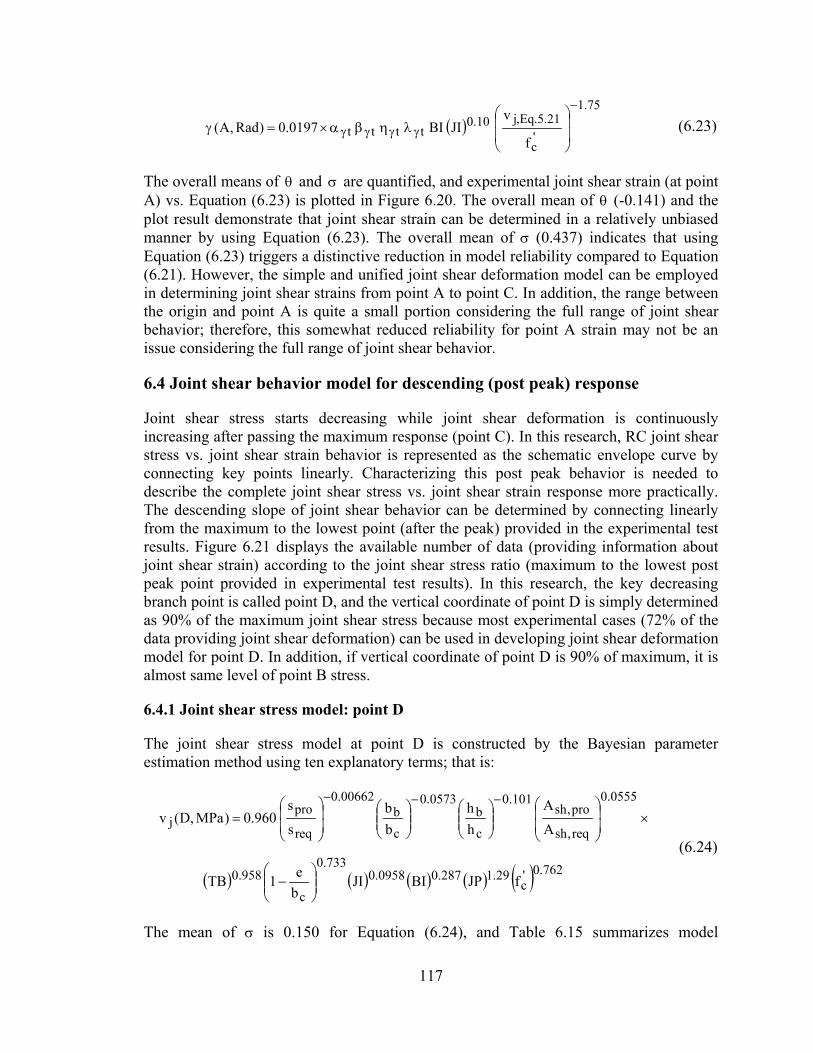
117

( )75.1

'c

21.5.Eq,j10.0tttt

f

vJIBI0197.0)Rad,A(

−

γγγγ ⎟⎟

⎠

⎞

⎜⎜

⎝

⎛ληβα×=γ (6.23)

The overall means of θ and σ are quantified, and experimental joint shear strain (at point A) vs. Equation (6.23) is plotted in Figure 6.20. The overall mean of θ (-0.141) and the plot result demonstrate that joint shear strain can be determined in a relatively unbiased manner by using Equation (6.23). The overall mean of σ (0.437) indicates that using Equation (6.23) triggers a distinctive reduction in model reliability compared to Equation (6.21). However, the simple and unified joint shear deformation model can be employed in determining joint shear strains from point A to point C. In addition, the range between the origin and point A is quite a small portion considering the full range of joint shear behavior; therefore, this somewhat reduced reliability for point A strain may not be an issue considering the full range of joint shear behavior.

6.4 Joint shear behavior model for descending (post peak) response

Joint shear stress starts decreasing while joint shear deformation is continuously increasing after passing the maximum response (point C). In this research, RC joint shear stress vs. joint shear strain behavior is represented as the schematic envelope curve by connecting key points linearly. Characterizing this post peak behavior is needed to describe the complete joint shear stress vs. joint shear strain response more practically. The descending slope of joint shear behavior can be determined by connecting linearly from the maximum to the lowest point (after the peak) provided in the experimental test results. Figure 6.21 displays the available number of data (providing information about joint shear strain) according to the joint shear stress ratio (maximum to the lowest post peak point provided in experimental test results). In this research, the key decreasing branch point is called point D, and the vertical coordinate of point D is simply determined as 90% of the maximum joint shear stress because most experimental cases (72% of the data providing joint shear deformation) can be used in developing joint shear deformation model for point D. In addition, if vertical coordinate of point D is 90% of maximum, it is almost same level of point B stress.

6.4.1 Joint shear stress model: point D

The joint shear stress model at point D is constructed by the Bayesian parameter estimation method using ten explanatory terms; that is:

( ) ( ) ( ) ( ) ( ) 762.0'c

29.1287.00958.0733.0

c958.0

0555.0

req,sh

pro,sh101.0

cb

0573.0

cb

00662.0

req

proj

fJPBIJIbe1TB

A

A

hh

bb

s

s960.0)MPa,D(v

⎟⎟⎠

⎞⎜⎜⎝

⎛−

×⎟⎟⎠

⎞⎜⎜⎝

⎛⎟⎟⎠

⎞⎜⎜⎝

⎛⎟⎟⎠

⎞⎜⎜⎝

⎛⎟⎟⎠

⎞⎜⎜⎝

⎛=

−−−

(6.24)

The mean of σ is 0.150 for Equation (6.24), and Table 6.15 summarizes model

118

uncertainty according to the procedure for removal of explanatory terms; the surviving parameters are the same as for points B, C, and D stress.

Due to the fact that joint shear stress at point D is 90% of joint shear strength, joint shear stress at point D could alternatively be expressed by multiplying 0.9 and Equation (5.19); that is:

( ) ( ) ( ) ( ) ( ) 761.0'c

290.1289.0097.0699.0

c957.0

052.0

req,sh

pro,sh101.0

cb

035.0

cb

010.0

req

proj

fJPBIJIbe1TB

A

A

hh

bb

s

s08.190.0)MPa,D(v

⎟⎟⎠

⎞⎜⎜⎝

⎛−

×⎟⎟⎠

⎞⎜⎜⎝

⎛⎟⎟⎠

⎞⎜⎜⎝

⎛⎟⎟⎠

⎞⎜⎜⎝

⎛⎟⎟⎠

⎞⎜⎜⎝

⎛×=

−−−

(6.25)

Finally, joint shear stress at point D could also be expressed by multiplying 0.9 and the simple and unified joint shear strength model (Equation (5.21)); that is:

( ) ( ) ( ) 75.0'c

30.015.0ttttj fBIJI90.0)MPa,D(v ληβα×= (6.26)

Table 6.15 Removal process: Total database except subassemblies with 0 in Ash ratio (point D stress)

1 2 3 4 5 6 7 8 9 10 'cf O O O O O O O O O O

JP O O O O O O O O O X

BI O O O O O O O O X X

JI O O O O O O O X X X

cbe1 − O O O O O O X X X X

TB O O O O O X X X X X

req,shpro,sh AA O O O O X X X X X X

cb hh O O O X X X X X X X

cb bb O O X X X X X X X X

reqpro ss O X X X X X X X X X

Mean of σ 0.150 0.150 0.150 0.150 0.151 0.158 0.164 0.186 0.230 0.373

6.4.2 Joint shear strain model: point D

Normalized joint shear strain model (joint shear strain to BI), which is for maintaining consistence in the development of joint shear strain models for other key points, for point D are constructed by the Bayesian parameter estimation method. Table 6.16 summarizes the removal process for point D strain. Because few experimental tests with

119

transverse beams provided descending slope, TB is not included in the surviving parameters. Same as the findings in Section 4.3.5, joint transverse reinforcement does not affect joint shear strain after peak. For point D strain, Equations (6.27a) and (6.27b) are the constructed joint shear strain models by considering all parameters and surviving parameters, respectively; those are:

( ) ( )

( ) 73.111.1

'c

j22.2

c

099.1

cb

292.0

req,sh

pro,sh

360.0

req

pro17.20676.00938.0

cb

JPRUf

)24.6(v

be1

bb

A

A

s

sTBJI

hh

BI0245.0)Rad,D(

−−−

−

⎟⎟

⎠

⎞

⎜⎜

⎝

⎛⎟⎟⎠

⎞⎜⎜⎝

⎛−⎟⎟

⎠

⎞⎜⎜⎝

⎛⎟⎟⎠

⎞⎜⎜⎝

⎛

×⎟⎟⎠

⎞⎜⎜⎝

⎛⎟⎟⎠

⎞⎜⎜⎝

⎛=γ

(6.27a)

( ) 99.141.1

'c

j50.1

cJPRU

f

)24.6(v

be1BI0115.0)Rad,D(

−−

⎟⎟

⎠

⎞

⎜⎜

⎝

⎛⎟⎟⎠

⎞⎜⎜⎝

⎛−=γ (6.27b)

The means of σ are 0.378 for Equation (6.27a) and 0.380 for Equation (6.27b), respectively.

Table 6.16 Removal process: Total database except subassemblies with 0 in Ash ratio (point D strain)

1 2 3 4 5 6 7 8 9 JPRU O O O O O O O O O

'cj f)24.6(v O O O O O O O O X

cbe1 − O O O O O O O X X cb bb O O O O O O X X X

req,shpro,sh AA O O O O O X X X X

reqpro ss O O O O X X X X X TB O O O X X X X X X JI O O X X X X X X X

cb hh O X X X X X X X X Mean of σ 0.378 0.376 0.378 0.378 0.379 0.379 0.380 0.406 0.517

If the average ratio of experimental joint shear strain (at point D) to Equation (6.7), for point C, is computed, then this calculated average (1.978) can simply be multiplied by Equation (6.7) to alternatively define joint shear strain at point D; that is:

( ) ( ) ( ) 01.257.1

'c

19.5.Eq,j01.2121.0712.0

c

403.0

req,sh

pro,sh257.0

cb

168.0

req

pro647.0

cb

JPRUf

vTBJI

be1

A

A

bb

s

s

hh

BI00653.0978.1)Rad,D(

−−

−−

⎟⎟

⎠

⎞

⎜⎜

⎝

⎛⎟⎟⎠

⎞⎜⎜⎝

⎛−

×⎟⎟⎠

⎞⎜⎜⎝

⎛⎟⎟⎠

⎞⎜⎜⎝

⎛⎟⎟⎠

⎞⎜⎜⎝

⎛⎟⎟⎠

⎞⎜⎜⎝

⎛×=γ

(6.28)

120

For Equation (6.28), the means of θ and σ are –0.113 and 0.390, respectively. Equation (6.28) indicates that joint shear deformation usually becomes almost twice that at the maximum strain during the 10% stress reduction from the maximum response. In addition, using Equation (6.28) does not result in a significant reduction in model reliability compared to Equation (6.27).

The average ratio of experimental joint shear strain (at point D) to the simple and unified joint shear deformation model (Equation (6.9)) is computed as 2.02. Equation (6.29) defines joint shear strain at point D by simply multiplying 2.02 to Equation (6.9); that is:

( )75.1

'c

21.5.Eq,j10.0tttt

f

vJIBI02.2)Rad,D(

−

γγγγ ⎟⎟

⎠

⎞

⎜⎜

⎝

⎛ληβα×=γ (6.29)

For Equation (6.29), the overall means of θ and σ are –0.106 and 0.401. As shown in Figure 6.22 (plotting experimental joint shear strain vs. joint shear strain defined by Equation (6.29)), Equation (6.29) can quite simply predict experimental joint shear strain (at point D) in an unbiased manner. The model uncertainty of Equation (6.29) is a little higher than that of Equation (6.27), however, the simple and unified model can be used all key points if point D strain is determined by Equation (6.29).

6.5 Summary of the developed joint shear behavior models

As described earlier, the schematic envelope curve of joint shear behavior can be determined by defining joint shear stress and joint shear strain at key points. Table 6.17 is the summary of the developed models by the Bayesian parameter estimation method employing all possible influence parameters. Table 6.18 is the summary of the suggested joint shear stress and strain models by adjusting the simple and unified joint shear strength and joint shear strain models at point C for the other key points.

Table 6.17 RC joint shear behavior model: Bayesian method for each point Developed model Eq. σ

( )

( ) ( ) ( ) ( ) 656.0'c

256.0

'c

c141.0458.0493.0372.0

c

106.0

cb

0191.0

req

pro0333.0

cb00814.0

00470.0

req,sh

pro,shj

ff

BIJPTBbe1

bb

s

s

hh

JIA

A731.0)(v

⎟⎟

⎠

⎞

⎜⎜

⎝

⎛ σ⎟⎟⎠

⎞⎜⎜⎝

⎛−⎟⎟

⎠

⎞⎜⎜⎝

⎛

×⎟⎟⎠

⎞⎜⎜⎝

⎛⎟⎟⎠

⎞⎜⎜⎝

⎛⎟⎟⎠

⎞⎜⎜⎝

⎛=

−−−A

(6.18) 0.134

( ) ( ) ( )08.2

'c

18.6.Eq,j93.1122.0

'c

c504.2247.0

c259.0

224.0

req

pro233.0

req,sh

pro,sh370.0

cb

174.0

cb

f

vJPRU

fTB

be1JI

s

s

A

A

hh

bb

BI0000329.0)(

−

−−

⎟⎟

⎠

⎞

⎜⎜

⎝

⎛

⎟⎟

⎠

⎞

⎜⎜

⎝

⎛ σ⎟⎟⎠

⎞⎜⎜⎝

⎛−

×⎟⎟⎠

⎞⎜⎜⎝

⎛⎟⎟⎠

⎞⎜⎜⎝

⎛⎟⎟⎠

⎞⎜⎜⎝

⎛⎟⎟⎠

⎞⎜⎜⎝

⎛=γ A

(6.21) 0.335

121

Table 6.17 (Cont’d) RC joint shear behavior model: Bayesian method for each point Developed model Eq. σ

( ) ( ) ( ) ( ) ( ) 768.0'c

27.1300.00623.0610.0

c09.1

0820.0

req,sh

pro,sh0715.0

cb

0433.0

cb

00861.0

req

proj

fJPBIJIbe1TB

A

A

hh

bb

s

s860.0)(v

⎟⎟⎠

⎞⎜⎜⎝

⎛−

×⎟⎟⎠

⎞⎜⎜⎝

⎛⎟⎟⎠

⎞⎜⎜⎝

⎛⎟⎟⎠

⎞⎜⎜⎝

⎛⎟⎟⎠

⎞⎜⎜⎝

⎛=

−−−

B (6.10) 0.149

( ) ( ) ( ) 85.187.1

'c

10.6.Eq,j249.007.1834.0

c

432.0

cb

193.0

req,sh

pro,sh164.0

req

pro405.0

cb

JPRUf

vJITB

be1

hh

A

A

s

s

bb

BI00189.0)(

−−

−−

⎟⎟

⎠

⎞

⎜⎜

⎝

⎛⎟⎟⎠

⎞⎜⎜⎝

⎛−

⎟⎟⎠

⎞⎜⎜⎝

⎛⎟⎟⎠

⎞⎜⎜⎝

⎛⎟⎟⎠

⎞⎜⎜⎝

⎛⎟⎟⎠

⎞⎜⎜⎝

⎛=γ B

(6.14) 0.365

( )

( ) ( ) ( ) ( ) 761.0c

290.1289.0097.0699.0

c

957.0052.0

req,sh

pro,sh101.0

cb

035.0

cb

010.0

req

proj

'fJPBIJIbe1

TBA

A

hh

bb

s

s08.1)(v

⎟⎟⎠

⎞⎜⎜⎝

⎛−

×⎟⎟⎠

⎞⎜⎜⎝

⎛⎟⎟⎠

⎞⎜⎜⎝

⎛⎟⎟⎠

⎞⎜⎜⎝

⎛⎟⎟⎠

⎞⎜⎜⎝

⎛=

−−−

C (5.19) 0.150

( ) ( ) ( ) 01.257.1

'c

19.5.Eq,j01.2121.0712.0

c

403.0

req,sh

pro,sh257.0

cb

168.0

req

pro647.0

cb

JPRUf

vTBJI

be1

A

A

bb

s

s

hh

BI00653.0)(

−−

−−

⎟⎟

⎠

⎞

⎜⎜

⎝

⎛⎟⎟⎠

⎞⎜⎜⎝

⎛−

×⎟⎟⎠

⎞⎜⎜⎝

⎛⎟⎟⎠

⎞⎜⎜⎝

⎛⎟⎟⎠

⎞⎜⎜⎝

⎛⎟⎟⎠

⎞⎜⎜⎝

⎛=γ C

(6.7) 0.394

( ) ( ) ( ) ( ) ( ) 762.0c

29.1287.00958.0733.0

c958.0

0555.0

req,sh

pro,sh101.0

cb

0573.0

cb

00662.0

req

proj

'fJPBIJIbe1TB

A

A

hh

bb

s

s960.0)(v

⎟⎟⎠

⎞⎜⎜⎝

⎛−

×⎟⎟⎠

⎞⎜⎜⎝

⎛⎟⎟⎠

⎞⎜⎜⎝

⎛⎟⎟⎠

⎞⎜⎜⎝

⎛⎟⎟⎠

⎞⎜⎜⎝

⎛=

−−−

D (6.24) 0.150

( ) ( )

( ) 73.111.1

'c

25.6.Eq,j22.2

c

099.1

cb

292.0

req,sh

pro,sh

360.0

req

pro17.20676.00938.0

cb

JPRUf

v

be1

bb

A

A

s

sTBJI

hh

BI0245.0)(

−−−

−

⎟⎟

⎠

⎞

⎜⎜

⎝

⎛⎟⎟⎠

⎞⎜⎜⎝

⎛−⎟⎟

⎠

⎞⎜⎜⎝

⎛⎟⎟⎠

⎞⎜⎜⎝

⎛

×⎟⎟⎠

⎞⎜⎜⎝

⎛⎟⎟⎠

⎞⎜⎜⎝

⎛=γ D

(6.27) 0.378

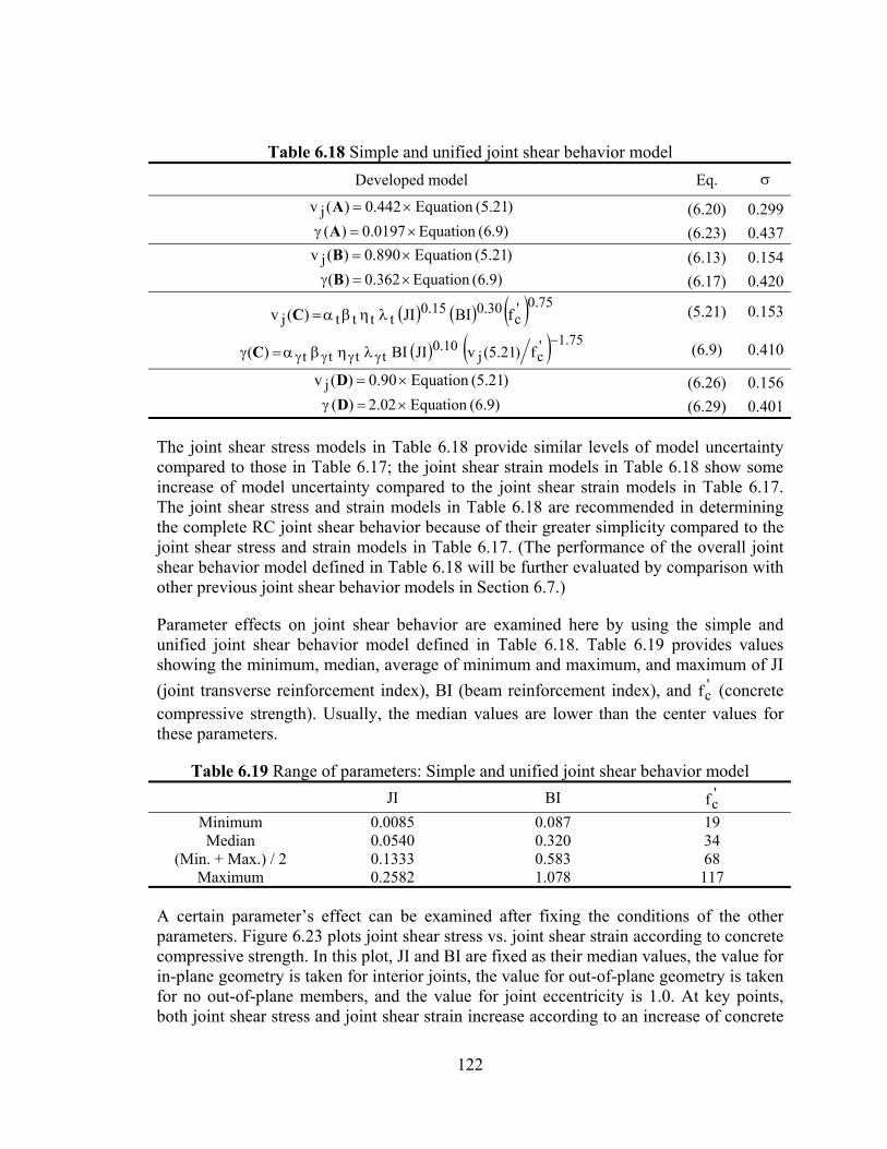
122

Table 6.18 Simple and unified joint shear behavior model Developed model Eq. σ

)21.5(Equation442.0)(v j ×=A (6.20) 0.299)9.6(Equation0197.0)( ×=γ A (6.23) 0.437)21.5(Equation890.0)(v j ×=B (6.13) 0.154

)9.6(Equation362.0)( ×=γ B (6.17) 0.420

( ) ( ) ( ) 75.0'c

30.015.0ttttj fBIJI)(v ληβα=C (5.21) 0.153

( ) ( ) 75.1'cj

10.0tttt f)21.5(vJIBI)(

−γγγγ ληβα=γ C (6.9) 0.410

)21.5(Equation90.0)(v j ×=D (6.26) 0.156)9.6(Equation02.2)( ×=γ D (6.29) 0.401

The joint shear stress models in Table 6.18 provide similar levels of model uncertainty compared to those in Table 6.17; the joint shear strain models in Table 6.18 show some increase of model uncertainty compared to the joint shear strain models in Table 6.17. The joint shear stress and strain models in Table 6.18 are recommended in determining the complete RC joint shear behavior because of their greater simplicity compared to the joint shear stress and strain models in Table 6.17. (The performance of the overall joint shear behavior model defined in Table 6.18 will be further evaluated by comparison with other previous joint shear behavior models in Section 6.7.)

Parameter effects on joint shear behavior are examined here by using the simple and unified joint shear behavior model defined in Table 6.18. Table 6.19 provides values showing the minimum, median, average of minimum and maximum, and maximum of JI (joint transverse reinforcement index), BI (beam reinforcement index), and '

cf (concrete compressive strength). Usually, the median values are lower than the center values for these parameters.

Table 6.19 Range of parameters: Simple and unified joint shear behavior model JI BI '

cf Minimum 0.0085 0.087 19 Median 0.0540 0.320 34

(Min. + Max.) / 2 0.1333 0.583 68 Maximum 0.2582 1.078 117

A certain parameter’s effect can be examined after fixing the conditions of the other parameters. Figure 6.23 plots joint shear stress vs. joint shear strain according to concrete compressive strength. In this plot, JI and BI are fixed as their median values, the value for in-plane geometry is taken for interior joints, the value for out-of-plane geometry is taken for no out-of-plane members, and the value for joint eccentricity is 1.0. At key points, both joint shear stress and joint shear strain increase according to an increase of concrete

123

compressive strength. Figure 6.24 plots joint shear stress vs. joint shear strain according to JI (with the other parameters fixed); an increase of JI triggers an improvement in joint shear stiffness. If JI is larger than the median value (the median value of JI is roughly equivalent to 0.70 in shA ratio), the effect of JI on joint shear behavior is attenuated. Figure 6.25 illustrates the effect of BI on joint shear behavior; an increase of BI results in an increase of both joint shear stress and strain, and BI’s effect on joint shear behavior is also attenuated when the value of BI is larger than the median. In Figure 6.26, the variable is the degree of joint eccentricity; a more flexible joint shear response is derived according to an increase of joint eccentricity, which is the opposite effect of JI on joint shear behavior response. Figures 6.27 and 6.28 plot joint shear behavior according to in-plane and out-of-plane geometry, respectively. These figures display that better geometry in resisting joint shear demand trigger an increase of both joint shear stress and strain.

For subassemblies within the database that provided experimental information about local and overall behavior, joint shear stress vs. joint shear strain have been plotted following the simple and unified joint shear behavior model (i.e. according to Table 6.18), and they are compared to the experimental results that provided information about local behavior in Appendix B. For example, Figure 6.29 presents a typical RC interior joint shear behavior (OKJ 1 tested by Noguchi and Kashiwazaki (1992)); based on visual comparison, the simple and unified RC joint shear behavior model is quite well-matched with the experimental joint shear behavior.

6.6 Subassemblies with no joint transverse reinforcement

An RC joint shear strength model for subassemblies with no joint transverse reinforcement was discussed back in Section 5.4; Equation (5.21) can still be applied to estimate joint shear strength for these subassemblies by using a virtual JI (of 0.0139). For the 7 out of 18 subassemblies with no joint transverse reinforcement that provided information about joint shear strain, the computed average ratio of experimental joint shear strain (at point C) to Equation (6.9) is 1.0 when tγλ is 0.00761 and JI is 0.0139.

In conjunction with Table 6.18, joint shear behavior at other key points for subassemblies with no joint transverse reinforcement can be defined by using the virtual JI (0.0139) instead of the actual JI (of zero) and 0.00761 instead of 0.00549 for tγλ . Table 6.20 shows the average of experiments with the suggested model at points A, B, and D for subassemblies with no joint transverse reinforcement.

This suggested approach is also almost unbiased in predicting joint shear stress at points A, B, and D. On the other hand, this method yields some bias in determining joint shear strain at points A, B, and D; however, the degree of bias is not significant. For the 7 subassemblies that have information about joint shear behavior, the suggested models can be compared to the experimental joint shear behavior, which are shown in Appendix B. The suggested model is quite accurate in describing experimental joint shear behavior. Obviously, more experimental test results are likely required in order to improve joint shear models for subassemblies with no joint transverse reinforcement.

124

Table 6.20 Average calculation: Subassemblies with no joint transverse reinforcement Point A Point B Point D

)23.6(Eq

(exp)jγ

)20.6(Eq

(exp)v j )17.6(Eq

(exp)jγ

)13.6(Eq

(exp)v j )29.6(Eq

(exp)jγ

)26.6(Eq

(exp)v j

Avg. 1.15 0.95 1.12 0.99 1.05 1.00

6.7 Performance evaluation: Joint shear behavior

The performance of the simple and unified RC joint shear behavior model (Table 6.18) is investigated here by comparison with other previous joint shear behavior models found in the literature, namely the FEMA 356 model, the Teraoka and Fujii model, the Parra-Montesinos and Wight model, and the MCFT. For subassemblies within the database having experimental information about joint shear stress vs. joint shear strain, the joint shear stress vs. joint shear strain have been plotted to visually examine the performance of the suggested model in this research, as provided in Appendix B. After visual comparison, the relatively improved performance of the simple and unified model has also been evaluated by quantifying the uncertainty of the various models.

6.7.1 FEMA 356 joint shear model

The Federal Emergency Management Agency (FEMA) provides guidelines for the seismic rehabilitation of existing structures (in FEMA 274); this document has been updated to applicable national pre-standard rule in FEMA 356 (“Prestandard and Commentary for the Seismic Rehabilitation of Buildings”, 2000).

Figure 6.30 shows the envelope model of RC joint shear stress vs. joint shear strain behavior subjected to seismic lateral loading, which is defined in Chapter 6 of FEMA 356. According to FEMA 356, the Y-axis value at point B is: “the resistance at 0.1QQ y = typically is the value at which the design shear strength is reached, and no strain hardening follows”. To determine the specific location of point B in joint shear behavior, the joint shear deformation (or AB slope) is needed. However, there is little information in FEMA 356 about that. Therefore, in this research, the X-coordinate of point B is not considered; thus, the FEMA 356 model is adjusted as shown in Figure 6.31.

FEMA 356 suggests the following joint shear strength definition; that is:

j'cn AfV γλ= (6.30)

Where, λ is a parameter considering concrete type (1.0 for normal weight aggregate concrete and 0.75 for lightweight aggregate concrete); γ is the joint shear strength factor; and jA is the effective joint shear area (same as the definition of ACI 318-05). Table 6.21 summarizes the joint shear strength factors defined in FEMA 356. Within the same geometric category (in-plane and out-of-plane), the joint shear strength factor is changed according to "ρ . This "ρ value is computed as )db(A effcs ×∑ , where ∑ sA is the total area of joint transverse reinforcement placed between the top and bottom beam

125

reinforcement in a connection (in the direction of loading); cb is the column width; and effd is the distance between the compressive and tensile resultants of the beam section.

For context, when the value of "ρ is around 0.003, the range of shA is from 0.53 to 0.96 within the total database. When "ρ is equal to or above 0.003 (probably considering modern joints), the joint shear strength factors defined by FEMA 356 are similar to the current ACI 352R-02 joint shear strength definition.

Table 6.21 Joint shear strength factor (FEMA 356) Joint shear strength factor ( γ : MPa0.5)

Interior with 2 transverse

beams

Interior without

transverse beams

Exterior with 2 transverse

beams

Exterior without

transverse beams

Knee

003.0" <ρ 1.00 0.83 0.67 0.5 0.33

003.0" ≥ρ 1.67 1.25 1.25 1.0 0.67

The FEMA 356 model also suggests joint shear deformation according to the joint condition, which is summarized in Table 6.22. In Table 6.22, the first column from the left is about column axial compression; P is the axial force and gA is the column cross-sectional area. The second column from the left is about the spacing of joint transverse reinforcement; C represents conforming joints (provided spacing of joint transverse reinforcement is equal to or smaller than 3hc ) and NC represents nonconforming joints (provided spacing of joint transverse reinforcement is larger than 3hc ). The third column from the left is about joint shear demand levels; V is the shear force and nV is the shear strength for the joint (Equation (6.30)).

For each experimental subassembly within the database that provided information about joint shear behavior, the joint shear behavior has been plotted following the FEMA 356 model, which is compared to the actual joint shear behavior defined by the experiment and also to the simple and unified joint shear behavior model of Table 6.18, as shown in Appendix B. For example, a typical RC interior joint shear behavior is shown in Figure 6.29. In general, the FEMA 356 model predicts joint shear behavior quite conservatively for most cases. For the FEMA 356 joint shear strength model, the overall means of θ and σ are evaluated. Then, experimental joint shear stress (at point C) vs. joint shear stress defined by the simple and unified model (Equation (5.21)) or the FEMA 356 model are plotted (Figure 6.32). The overall mean of θ (0.310) and the plot results confirm that the FEMA 356 joint shear strength model is conservative in determining joint shear strength. In addition, the FEMA 356 model has less model reliability with respective to joint shear strength compared to the simple and unified model.

The FEMA 356 model defines plastic joint shear deformation (“a”), which is mainly dependent on in-plane geometry and the spacing of joint transverse reinforcement. From experimental tests and the simple and unified joint shear model (Table 6.18), plastic joint shear deformations can be computed by subtracting the point B strain from the point C

126

strain. Figure 6.33 plots experimental plastic joint shear deformation vs. plastic joint shear deformation defined by Table 6.18 and the FEMA 356 model. As shown in this figure, FEMA’s constant values cause a large scatter in determining plastic joint shear deformation. For example, the range of experimental plastic deformation is from 0.001 to 0.035 when the FEMA 356 defines “a” as 0.015.

Table 6.22 Joint shear deformation (FEMA 356) Interior joints

)fA(N 'cg × Transv. Reinf. nVV “a” “b” “c”

≤ 0.1 C ≤ 1.2 0.015 0.03 0.2 ≤ 0.1 C ≥ 1.5 0.015 0.03 0.2 ≥ 0.4 C ≤ 1.2 0.015 0.025 0.2 ≥ 0.4 C ≥ 1.5 0.015 0.02 0.2 ≤ 0.1 NC ≤ 1.2 0.005 0.02 0.2 ≤ 0.1 NC ≥ 1.5 0.005 0.015 0.2 ≥ 0.4 NC ≤ 1.2 0.005 0.015 0.2 ≥ 0.4 NC ≥ 1.5 0.005 0.015 0.2

Other joints )fA(N '

cg × Transv. Reinf. nVV “a” “b” “c” ≤ 0.1 C ≤ 1.2 0.01 0.02 0.2 ≤ 0.1 C ≥ 1.5 0.01 0.015 0.2 ≥ 0.4 C ≤ 1.2 0.01 0.02 0.2 ≥ 0.4 C ≥ 1.5 0.01 0.015 0.2 ≤ 0.1 NC ≤ 1.2 0.005 0.01 0.2 ≤ 0.1 NC ≥ 1.5 0.005 0.01 0.2 ≥ 0.4 NC ≤ 1.2 0.0 0.0 - ≥ 0.4 NC ≥ 1.5 0.0 0.0 -

6.7.2 Teraoka and Fujii model

Teraoka and Fujii (2000) suggested a joint shear stress vs. joint shear strain model based on their collected experimental test results. In their model, RC joint shear behavior is described by four defined points A, B, C, and D, which are summarized as follows:

Cracking joint shear stress is derived using stress coordinate transformation, and joint shear strain is computed by joint shear stress divided by shear modulus of concrete; those are:

ot2

tj ff)MPa,A(v σ+= (6.31) G)A(v)A( j=γ (6.32)

where, tf is the tensile strength of concrete (= 'cf4.0 , MPa), 0σ is the column axial

stress, and G is the shear modulus of concrete. (These are similar to the developed equations for joint cracking stress and strain back in Section 4.2.)

Teraoka and Fujii considered that joint shear behavior is distinctively changed

127

when the joint shear stress reaches about 85% of the ultimate joint shear strength; those are:

)C(v85.0)B(v jj = (6.33) 004.0)B( =γ (6.34)

At maximum response (point C), joint shear stress and joint shear strain are defined as Equations (6.35) and (6.36); those are:

jj Fk)C(v φ= (6.35) 01.0)C( =γ (6.36)

In Equation (6.35), k is the factor describing in-plane geometry (1.0 for interior joints, 0.7 for exterior joints, and 0.4 for knee joints); φ is the factor describing out-of-plane geometry (1.15 for joints with 2 transverse beams and 1.0 for other types); and jF is the

standard value of joint shear strength ( ( ) 7.0'cf8.0 × , MPa). The effective joint shear area of

this model is same as the definition of AIJ 1999; the effective joint width ( jb ) is defined as 2a1abj bbbb ++= ( 1ab , 2ab : the smaller of one-quarter of column depth and one-half of distance between beam and column face on either side of beam) and the effective joint shear depth ( jD ) is simply defined as the column depth for an interior connection, or the projected development length of anchored beam bars with 90 degree hooks for exterior and knee joints.

In the Teraoka and Fujii model, post-peak joint shear behavior is described in Equations (6.37) and (6.38); those are:

)C(v80.0)D(v jj ×= (6.37) 02.0)D( =γ (6.38)

For visual comparison, joint shear stress vs. joint shear strain behavior is plotted following the Teraoka and Fujii model, and it is compared to the experimental and the simple and unified joint shear behavior model in Appendix B; one typical RC joint shear behavior, for example, is shown in Figure 6.29.

For joint shear strength defined by the Teraoka and Fujii model, the overall means of θ and σ are evaluated by using all cases (expect subassemblies with no joint transverse reinforcement) within the database (because they did not explain any limitation in joint confinement in their model); the computed overall means of θ and σ are –0.245 and 0.231. Figure 6.34 plots experimental joint shear stress vs. joint shear stress (at point C) as defined by Equation (5.21) or the Teraoka and Fujii model. As shown in this figure, their not-conservative cases are usually subassemblies with below 0.70 in shA ratio. This means that the performance of joint shear strength as defined by Teraoka and Fujii might be improved if the subassemblies with equal to or above 0.70 in shA ratio are only included (the overall means of θ and σ are 0.127 and 0.199, respectively) or if a

128

factor accounting for proper joint confinement were included in their model.

For the joint shear strain defined by Teraoka and Fujii at point C, the overall means of θ and σ are –0.195 and 0.563, respectively. Figure 6.35 plots experimental joint shear strain vs. joint shear strain defined by Equation (6.9) or the Teraoka and Fujii model. These examination results indicate that using a constant value for joint shear strain is not reasonable in determining joint shear deformation. (When using subassemblies with equal to or above 0.70 in shA ratio, the overall means of θ and σ are –0.327 and 0.485, respectively.)

6.7.3 Parra-Montesinos and Wight model

Parra-Montesinos (2000) originally suggested an analytical approach for estimating joint shear behavior of composite RC column-to-steel beam connections, and this type of approach has been continuously applied in his research. In his approach, principal joint shear strain is defined in the joint panel by relating principal tensile and compressive strains. Parra-Montesinos and Wight (2002) adjusted this analytical approach for estimating joint shear behavior of RC beam-column connections. They considered that joint shear strength is provided by an equivalent diagonal compression strut activated by force transfer to the joint by direct bearing from the beam and column compression zones and by bond between the beam and column reinforcement and the surrounding concrete, which is shown in Figure 6.36. In their suggested model, the shape of this equivalent concrete strut was determined by the geometry and reinforcement array of the beams and columns. For the in-plane and out-of-plane directions, the dimensions of the equivalent strut are expressed in Equations (6.39) and (6.40); that is:

2c

2intjo

cintjostrut

hd

hdd

+= (in-plane direction) (6.39)

2bb

b cbstrut

+= (out-of-plane direction) (6.40)

In Equation (6.39), intjod ( 'dd − ) is the distance between the top and the bottom beam reinforcement.

In their suggested method, the principal compressive direction is assumed to be the same as the direction of the “diagonal equivalent strut”; that is:

⎟⎟⎠

⎞⎜⎜⎝

⎛=θ −

c

intjo1strut h

dtan (6.41)

Parra-Montesinos and Wight first suggested a possible relation between joint shear strain and principal strain ratio based on their nine collected experimental test results; that is:

γ+= stc k2K (6.42)

129

In Equation (6.42), tcK is the ratio of principal tensile strain to principal compressive strain ( ct εε− ); γ is the joint shear strain; and sk is the suggested slope for the tcK vs. γ relationship ( cs be2000500k += , e : amount of joint eccentricity). Parra-Montesinos and Wight commented that Equation (6.42) is valid only up to about 1% joint shear deformation for subassemblies maintaining proper confinement within the joint panel, because they derived this relation based on these specific nine experimental test results. They recommended that more data are needed to derive general relations between the principal strain ratio and joint shear deformation.

Plane strain within the joint panel can be expressed as the following 3 equations, using strain coordinate transformation; that is:

)2sin(2

)2cos(22

yxyxc θ

γ+θ

ε−ε+

ε+ε=ε (6.43)

)]90(2sin[2

)]90(2cos[22

K yxyxctct +θ

γ++θ

ε−ε+

ε+ε=ε−=ε (6.44)

))(2tan( yx ε−εθ=γ (6.45)

where xε , yε , cε , and tε are the strains for the X, Y, principal compressive, and principal tensile directions, respectively. When joint shear strain ( γ ) is given and the principal strain direction ( θ ) is known, four plane strains ( xε , yε , cε , and tε ) can be determined by employing Equations (6.42), (6.43), (6.44), and (6.45).

In the calculation of the principal compressive stress of the equivalent strut, the compression softening parameter (β ) is applied; that is:

tcK27.085.01

+=β (6.46)

Different from the original suggestion of Vecchio and Collins (1993), Parra-Montesinos and Wight set the lowest boundary of β = 0.6.

To find the principal compressive stress at the calculated principal compressive strain, Parra-Montesinos and Wight employed the concrete stress vs. strain model proposed by Sheikh and Uzumeri (1982). Figure 6.37 displays the concrete stress vs. strain model suggested by Sheikh and Uzumeri, after applying the compression softening factor suggested by Vecchio and Collins. In this concrete stress vs. strain model, sK is a factor that accounts for the increase in the compressive strength of confined concrete; that is:

'ss

22

2

occ

2s f])

B2s1)(

B5.5

Cn1[(P140

B0.1K ρ−−+= (6.46)

where B is the horizontal center-to-center distance of the perimeter ties of a rectangular core (mm); n is the number of arcs (number of longitudinal column

130

reinforcement); C is the center-to-center distance between longitudinal column reinforcement (mm); s is the vertical spacing of tie reinforcement (mm); sρ is the volumetric tie reinforcement ratio; 'fs is the yield stress of tie reinforcement (MPa); and

occP is computed as ( )( ) 1000AA'f85.0 scc ∑− , where cA is the column cross-sectional area, and ∑ sA is the total amount of column reinforcement. This concrete stress-strain curve consists of 4 segments as follows:

OA region: Ascending (parabolic) part ( cε is lower than or equal to 1sε )

6'cs1s 10fK80 −×=ε (6.47)

'cscc fKf β= (6.48)

])(2[ff 2

1s

c

1s

cccc ε

ε−

εε

= (6.49)

AB region: Plateau (flat) part ( cε is between 1sε and 2sε )

'c

'ss22s

f

f])

Bs(0.51[

C2481

0022.0ρ

−+=ε (6.50)

ccc ff = (6.51)

BC region: Descending (linear) part ( cε is above 2sε )

sB

43

5.0Z

sρ=

(6.52)

)](Z1[ff 2scccc ε−ε−= (6.53)

CD region: Lower (flat) plateau part (residual stress)

ccc f3.0f = (6.54)

After computing the principal compressive stress, the diagonal strut resistance can be computed as Equation (6.55), and then the horizontal component of diagonal force is computed as Equation (6.56); those are:

intjointjoccstrut db)(fC ε= (6.55) )(cosCV strutjh θ= (6.56)

In Appendix B, joint shear stress vs. joint shear strain is plotted according to the procedure proposed by Parra-Montesinos and Wight, up to 1% joint shear deformation, for interior and exterior connections with equal to or above 0.70 in shA ratio and with no out-of-plane members (due to the limitations of their method); one example is shown in Figure 6.29. Joint shear stress is continuously increased up to 1% joint

131

shear strain. For the joint shear strength defined by Parra-Montesinos and Wight, the overall means of θ and σ (to check model reliability) are 0.190 and 0.359, respectively. Figure 6.38 also plots experimental joint shear stress vs. joint shear stress defined by Equation (5.21) or the Parra-Montesinos and Wight model. Joint shear strength (defined by Parra-Montesinos and Wight) appears to be determined too conservatively, in part due to Equation (6.42) and the upper limit (1%) on joint shear deformation.

For the joint shear deformation by Parra-Montesinos and Wight, at maximum, the overall means of θ and σ are computed as 0.422 and 0.410, respectively. At maximum response, experimental joint shear strain vs. joint shear strain defined by Parra-Montesinos and Wight or Equation (6.9) is plotted in Figure 6.39. The constant upper limit (1%) of joint shear deformation is apparently not reasonable in determining joint shear deformation at maximum response.

6.7.4 Modified Compression Field Theory (MCFT)

Vecchio and Collins (1986) have suggested the Modified Compression Field Theory (MCFT) to predict the response of two-dimensional (2D) RC membrane elements subjected to shear and normal stress. Youssef and Ghobarah (2001), Lowes and Altoontash (2003), and Shin and LaFave (2004) considered that joint shear behavior might also be similar to the shear behavior of a 2D RC membrane element. So, they employed the MCFT to describe RC joint shear behavior in conjunction with overall modeling of RC beam-column connections.

The MCFT models cracked concrete using a smeared rotating crack approach. Thus, the relationships are formulated in terms of average stresses and strains. The basic assumptions of the MCFT are as follows: reinforcement and cracking are distributed uniformly; shear and normal stress are applied to an RC membrane element uniformly; reinforcement and concrete are connected by perfect bond; the stress state is unique for each strain state; and the orientation of principal stress coincides with the orientation of principal strain. Based on these assumptions, Vecchio and Collins suggested the MCFT using strain compatibility, force equilibrium, and constitutive relationships for average stress and strain. Some key characteristics of the MCFT are the following: compression softening due to tensile strain, tension stiffening due to perfect bond between concrete and reinforcement, and shear contribution of local stress and strain at cracks. The MCFT has three limitations, namely: first, average principal tensile stress is limited by reinforcement yielding at a crack face; second, shear stress is limited by the aggregate interlock mechanism at a crack face; and third, average principal compressive stress is limited by softened compressive stress.

Vecchio and Collins (1986) provided the solution technique for determining the response of bi-axially stressed elements (in the appendix of their paper), which can be summarized as follows:

132

Step 1: Choose a principal tensile strain ( 1ε )

Step 2: Estimate the principal compressive stress direction ( θ )

Step 3: Calculate the average crack width ( w ) at a given 1ε and θ

mymx scos

ssin

1sθ

+θ

=θ (6.57)

where mxs and mys are the average spacing of cracks perpendicular to the x and y reinforcement, respectively; mxs is 1.5 times the maximum distance of x-bars and mys is 1.5 times the maximum distance of y-bars. The crack width ( w ) is then calculated in Equation (6.58); that is:

θε= sw 1 (6.58)

Step 4: Estimate average stress in the weaker reinforcement; e.g., if the y-direction is weaker, assume an average stress of the y-direction reinforcement ( syf )

Step 5: Compute the average tension in the concrete ( 1cf )

1c1c Ef ε= (before cracking) (6.59)

1

cr1c

2001f

fε+

= (after cracking) (6.60)

where cE is the modulus of elasticity of concrete and crf is the concrete cracking stress. Equation (6.61) can be derived from the static equivalency between the calculated average stresses and the actual local stresses at the cracks; that is:

( ) θ+−−ρ= tanvffff cicisysycrsy1c (6.61)

where syρ is the reinforcement ratio in the y-direction; sycrf is the stress in the y-reinforcement at the crack location; cif is the compressive stress at the crack surface; and

civ is the shear stress at the crack surface. Shear stress at the crack surface can be expressed as the following equation; that is:

maxci

2ci

cimaxcici vf

82.0f64.1v18.0v −+= (6.62)

)16a(w2431.0

'fv c

maxci

++

−= ( '

cf : negative for compression) (6.63)

133

In Equation (6.63), a is the maximum aggregate size (mm).

In the MCFT, the average principal tensile stress is limited by reinforcement yielding at the crack face. Thus, sycrf is equal to yyf (yield stress of y-reinforcement) in the limit condition. Equation (6.61) can be expressed by considering Equation (6.62) and yyf instead of sycrf , that is:

( ) θ⎟⎟

⎠

⎞

⎜⎜

⎝

⎛−⎟

⎠⎞

⎜⎝⎛

θ−++−ρ= tan

v

f82.0

vf

tan164.118.0vfff

2maxci

2ci

maxcici

maxcisyyysy1c (6.64)

Let k)tan164.1( =θ− and Xvf maxcici = . Then, 2X82.0kX − can be transformed into Equation (6.65); that is:

22

2 k3.064.1kX82.0X82.0kX +⎟

⎠⎞

⎜⎝⎛ −−=− (6.65)

For maximum, X is equal to 64.1k . Thus, Equation (6.64) can be finally expressed as Equation (6.66); that is:

( ) ( ) θ++−ρ= tank3.018.0vfff 2maxcisyyysy1c (6.66)

Therefore, cif should be equal to or smaller than Equation (6.66).

Step 6: Calculate shear stress ( xyv ) from force equilibrium

sysyycy fff ρ−= (6.67) ( ) θ−= tan/ffv cy1cxy (6.68)

where yf is the stress applied to the element in the y-direction.

Step 7: Calculate principal compressive stress in concrete ( 2cf )

( )θ+θ−= tan1tanvff xy1c2c (6.69)

Step 8: Calculate max2cf at a given 1ε

0.1

'34.08.0

1'f

f

c1c

max2c ≤

ε−

=ε

(6.70)

In Equation (6.70), 'cε is the strain in concrete cylinders at peak stress (usually –0.002). If 'ff cmax2c is greater than 1.0, return to Step 2 and choose a lower 1ε . If

134

'ff cmax2c is equal to or less than 1.0, go to the next step.

Step 9: Calculate principal compressive strain ( 2ε )

( )max2c2cc2 ff11' −−ε=ε (6.71)

Step 10: Compute strain in the y-direction ( yε )

( )( )2

221

ytan1

tan

θ+

θε+ε=ε (6.72)

Step 11: Calculate average stress in the y-direction ( updated,fsy = yyys fE ≤ε )

If updated,fsy is equal to syf , move to the next step. If updated,fsy is not equal to syf , return to Step 4.

Step 12: Compute strain in the x-direction ( xε = y21 ε−ε+ε )

Step 13: Calculate average stress in the x-direction ( sxf = yxxs fE ≤ε )

Step 14: Calculate cal,xf from force equilibrium

θ−= tanvff xy1ccx (6.73) sxsxcxcal,x fff ρ+= (6.74)

If cal,xf is equal to xf (stress applied to element in the x-direction), go to the next step. If

cal,xf is not equal to xf , return to Step 2.

Step 15: Compute civ and cif

From Equation (6.61), civ can be computed in Equation (6.75); that is:

( )1c1cci fftan

1v Δ+θ

= (6.75)

where 1cfΔ is ( )syyysyci fff −ρ−

Equation (6.62) can be expressed as Equation (6.76); that is:

( ) ( ) 0v18.0tan

ff64.1

tan1f

v82.0

maxcici

ci2

cimaxci

=−θ

Δ+⎟

⎠⎞

⎜⎝⎛ −

θ+ (6.76)

135

Let Av82.0 maxci = , ( ) B64.1tan1 =−θ , and Cv18.0tanf maxcici =−θΔ . Then, cif can be computed as follows; that is:

A2

AC4BBf

2

ci

⎟⎠⎞

⎜⎝⎛ −−−

= (6.77)

If 1cfΔ is smaller than 0, go to the next step.

Step 16: Calculate reinforcement stress ( sxcrf , sycrf )

( ) sxcici1csxsxcr tanvffff ρθ+++= (6.78) ( ) sycici1csxsycr tanvffff ρθ−++= (6.79)

If sxcrf and sycrf are equal to or smaller than yxf and yyf , respectively, move to the next step. Otherwise, go to step 6.

Step 17: Compute shear strain ( xyγ )

( )θε−ε

=γtan

2 2xxy (6.80)

Joint shear behavior has been computed using “Membrane 2000” that aims at analyzing a 2D RC membrane element based on MCFT (Bentz and Collins, 2001). In these analyses, a joint panel is considered as one element and the boundary condition around of the joint panel is also simplified (no consideration about bending). Because the MCFT assumes that reinforcement is uniformly distributed within an element, beam (top and bottom) reinforcement is also not considered in the MCFT analysis. Joint transverse reinforcement is considered as the only effective x-direction reinforcement. The joint transverse reinforcement ratio is defined as the total amount of joint transverse reinforcement, which is located between the top and bottom beam reinforcement, divided by the product of the column width and effective height (the distance between top and bottom beam reinforcement). Longitudinal column reinforcement is considered as the effective y-direction reinforcement. The column reinforcement ratio is defined as the total amount of longitudinal column reinforcement divided by the column cross-sectional area. Normal stresses of X and Y direction is computed by axial compression to cross-sectional area. The maximum aggregate size is fixed as 19 mm in all analysis because of lack of information in experimental papers and reports. Within the constructed database (of strong-column / weak-beam designed specimens), the X-direction is weaker than the Y-direction; thus, the MCFT analysis result might usually be more influenced by the reinforcement condition in the X-directions, which is also explained by Shin and LaFave (2004) and Lowes and Altoontash (2003).

In Appendix B, the joint shear stress vs. joint shear strain defined by the MCFT is plotted, and it is compared to the joint shear behavior defined by each experiment and by Table

136

6.18; one example is shown in Figure 6.29. In general, the MCFT generally predicts RC joint shear behavior conservatively.

For RC joint shear strength defined by the MCFT, the overall means of θ and σ are 0.261 and 0.372, respectively. The plot result of Figure 6.40 (experimental joint shear stress vs. joint shear stress defined by the MCFT or Equation (5.21)), as well as the overall mean of θ , indicate that the MCFT is conservative in determining RC joint shear strength because it might ignore the contribution of beam reinforcement.

For joint shear deformation defined by the MCFT at maximum response, the overall means of θ and σ are 0.951 and 0.795, respectively. Figure 6.41 also plots experimental joint shear strain vs. joint shear strain defined by the MCFT and Equation (6.9) at maximum response. These examination results show that the joint shear deformations defined by the MCFT are usually smaller than experimental results.

6.8 Modified Parra-Montesinos and Wight model

The Parra-Montesinos and Wight model has been modified in conjunction with the constructed database. The reasonableness of their assumptions has first been reviewed. Then, the identified deficiency of their model is modified using the database. Finally, the performance of the modified Parra-Montesinos and Wight model is evaluated.

Equivalent strut direction and shape: Due to the fact that there is no clear method for quantifying bond capacity after several cyclic loadings in macro modeling (one element as a joint panel), Parra-Montesinos and Wight assumed a fixed equivalent strut direction and shape. In this research, the fixed direction and shape of the equivalent strut is also employed. After fixing the direction and shape of the equivalent strut, the effect by bond condition may be indirectly considered in the derived relation between the principal strain ratio and the joint shear strain.

Relation between the principal strain ratio and joint shear deformation: Parra-Montesinos and Wight used only nine subassemblies; therefore, their derived relation between the principal strain ratio and the joint shear deformation may not correctly describe diverse conditions of RC beam-column connections. In this research, this relationship is modified in conjunction with the constructed database to predict joint shear behavior for diverse types of RC beam-column connections.

Concrete constitutive model: Parra-Montesinos and Wight applied the concrete stress vs. strain model proposed by Sheikh and Uzumeri (1982) for RC columns. A joint panel is considered as a part of an RC column in the current design philosophy, so, using the concrete constitutive model by Sheikh and Uzumeri seems reasonable.

Compression softening factor: Differing from the suggestion of Vecchio and Collins (1993), Parra-Montesinos and Wight suggested a lowest boundary value for the concrete compression softening factor (=0.6). The original method proposed by Vecchio and Collins is applied in this research.

137

As shown above, the most deficient point of the Parra-Montesinos and Wight model is in the relation between the principal strain ratio and the joint shear deformation. From the constructed database, then, the principal strain ratio is computed at a given experimental joint shear strain employing the following procedure.

Step 1: Determine the “equivalent strut shape” and the principal compression direction ( θ )

Step 2: Select joint shear strain ( γ ) from the experimental test

Step 3: Choose a trial principal strain ratio ( tcK = ct εε− )

Step 4: Compute the plane strain ( xε , yε , cε , tε ) using Equations (6.43), (6.44), and (6.45)

Step 5: Compute the compression softening factor using Equation (6.46)

Step 6: Compute the principal compressive stress ( cσ ) at the calculated cε

The principal compressive stress is computed employing the concrete stress vs.

strain model proposed by Sheikh and Uzumeri in conjunction with the

compression softening factor determined in Step 5.

Step 7: Compute the diagonal compression of the equivalent strut

Step 8: Compute the horizontal component of the diagonal compression

Step 9: Compare the experimental and the computed joint shear

Return to Step 3 and choose a new tcK until the computed joint shear is equal to the experimental joint shear

Step 10: Go to Step 2 for a new joint shear strain

The principal strain ratio ( tcK ) is specifically computed at key points of joint shear behavior (points A, B, C, and D). In general, the computed principal strain ratio is proportional to joint shear deformation, which is shown for example in Figure 6.42 (for an interior connection with no-out-of plane members and no joint eccentricity). The plot of computed principal strain ratio vs. experimental joint shear strain (of Figure 6.42) is simplified as Figure 6.43 because the region between points B and C generally comprises about 64% of the maximum joint shear deformation (point C), as shown in Table 6.18. The slope between points B and C is extended back to 0 for joint shear strain. In

138

Figure 6.43, the principal strain ratio at zero joint shear strain is referred to as the initial principal strain ratio ( i,tcK ), and the slope is referred to as the principal strain ratio slope ( s,tcK ). Under this simplification, both initial principal strain ratio and the principal strain ratio slope are found for each subassembly that provides information about joint shear behavior. The key relation between the principal strain ratio and the joint shear strain can be expressed as Equation (6.81); that is:

γ×+= s,tci,tctc KKK (6.81)

Equations for the initial principal strain ratio ( i,tcK ) and the principal strain ratio slope ( s,tcK ) have been constructed using the experimental database in conjunction with the Bayesian parameter estimation method. In constructing un-biased i,tcK and s,tcK , nine explanatory terms ( shA ratio, spacing ratio, beam width to column width, beam height to column depth, joint transverse reinforcement index, beam reinforcement index, joint eccentricity, out-of-plane geometry, and in-plane geometry) are employed. After removing insignificant influence parameters, the constructed i,tcK and s,tcK can be expressed as Equations (6.82) and (6.83), respectively.

( ) ( ) ( ) ( ) 711.038.2

c14.4362.0062.0

i,tc JPbe1TBBIJI96.2K −

−−

⎟⎟⎠

⎞⎜⎜⎝

⎛−= (6.82)

( ) ( ) ( ) ( ) 88.1678.0235.0408.00846.0

cs,tc JPBIJITB

be142.41K −−−−

⎟⎟⎠

⎞⎜⎜⎝

⎛−= (6.83)

The means of σ are 0.70 for Equation (6.82) and 0.507 for Equation (6.83).

The initial principal strain ratio can be simplified into Equation (6.84); that is:

( ) ( ) 362.0062.0iiiii,tc BIJIK ληβα= (6.84)

In Equation (6.84), iα is a parameter describing in-plane geometry (1.0 for interior, 1.23 for exterior, and 1.64 for knee); iβ is a parameter describing out-of-plane geometry (1.0

for 0 and 1 transverse beam and 0.47 for 2 transverse beams); iη (= ( ) 38.2cbe1 −− ) is a

parameter describing joint eccentricity; and iλ is 2.958 in order to have 1.0 as the average of Equations (6.82) through (6.84). When employing Equation (6.84), the overall means of θ and σ are –0.355 and 0.699, respectively.

The principal strain ratio slope can also be simplified, as Equation (6.85); that is:

( ) ( ) 678.0235.0sssss,tc BIJIK −−ληβα= (6.85)

In Equation (6.85), sα is a parameter describing in-plane geometry (1.0 for interior, 1.72

139

for exterior, and 3.68 for knee); sβ is a parameter describing out-of-plane geometry (1.0

for 0 and 1 transverse beam and 0.93 for 2 transverse beams); sη (= ( ) 0846.0cbe1 − ) is a

parameter describing joint eccentricity; and sλ is 42.4 in order to have 1.0 as the average of Equations (6.83) through (6.85). When employing Equation (6.85), the overall means of θ and σ are –0.120 and 0.701, respectively.

RC beam-column connection joint shear stress vs. joint shear strain can now be predicted by employing the modified Parra-Montesinos and Wight model utilizing the following steps:

Step 1: Determine the “equivalent strut shape” and the principal compression direction ( θ )

Step 2: Select joint shear strain ( γ )

Step 3: Compute the principal strain ratio at a given joint shear strain (using Equation

(6.81))

The initial principal strain ratio ( i,tcK ) is calculated using Equation (6.84) and the principal strain ratio slope ( s,tcK ) is computed using Equation (6.85).

Step 4: Compute the plane strain ( xε , yε , cε , tε ) using Equations (6.43), (6.44), and (6.45)

Step 5: Compute the compression softening factor using Equation (6.46)

Step 6: Compute principal compressive stress ( cσ ) at the calculated cε

The principal compressive stress is computed employing the concrete stress vs.

strain model proposed by Sheikh and Uzumeri in conjunction with the

compression softening factor determined in Step 5.

Step 7: Compute the diagonal compression of the equivalent strut

Step 8: Compute the horizontal component of the diagonal compression

Step 9: Go to Step 2 for a new joint shear strain

For each subassembly that has information about joint shear behavior, the joint shear stress vs. joint shear strain behavior is plotted following the modified Parra-

140

Montesinos and Wight model, which is provided in Appendix B; Figure 6.29, for example, represents a typical RC interior joint shear behavior. Based on visual comparison, the modified Parra-Montesinos and Wight model improve accuracy in the prediction of RC joint shear behavior compared to the original Parra-Montesinos and Wight model.

For maximum stress, the modified Parra-Montesinos and Wight model provides that the overall means of θ and σ are –0.031 and 0.215, respectively. As shown in Figure 6.44, the model reliability of this modified model is still lower than that of the simple and unified model (the overall means of θ and σ are –0.018 and 0.155, respectively). However, the model reliability of this modified model is distinctively improved compared to the original Parra-Montesinos and Wight model (the overall means of θ and σ are 0.190 and 0.359, respectively).

For maximum strain, the modified Parra-Montesinos and Wight model shows that the overall means of θ and σ are 0.311 and 0.467, respectively. Under the same data groups, the modified Parra-Montesinos and Wight model shows that the overall means of θ and σ are 0.270 and 0.372, respectively; the modified model is less biased and more reliable than the original model (the overall means of θ and σ are 0.422 and 0.410, respectively). Same as the finding for maximum stress, the simple and unified joint shear behavior model is more reliable than this modified model (Figure 6.45).

6.9 Summary of RC joint shear behavior models

In Chapter 6, complete RC joint shear behavior models, which are applicable for diverse types of RC beam-column connections, have been suggested. In addition, current existing models to define the envelope of complete RC joint shear behavior are also explained in detail. Table 6.23 summarizes the overall means of θ and σ at maximum response for six approaches: the FEMA 356 model, the Teraoka and Fujii model, the Parra-Montesinos and Wight model, the MCFT, the modified Parra-Montesinos and Wight model, and the simple and unified joint shear behavior model (Table 6.18). Among these six models, the simple and unified RC joint shear behavior model is the most reliable in determining maximum response (point C). In general, existing models determine maximum response in a conservative direction. Except for the simple and unified joint shear behavior model (Table 6.18), the modified Parra-Montesinos and Wight is more reliable than other approaches.

Table 6.23 Posterior mean of the joint shear behavior model (at maximum response) Stress Strain Posterior mean Posterior mean θ σ θ σ

FEMA 356 0.310 0.292 Teraoka and Fujii -0.245 0.231 -0.195 0.563

Parra-Montesinos and Wight 0.190 0.359 0.422 0.410 MCFT 0.261 0.372 0.951 0.795

Modified Parra-Montesinos and Wight -0.031 0.215 0.311 0.467 Table 6.18 -0.016 0.153 -0.117 0.410

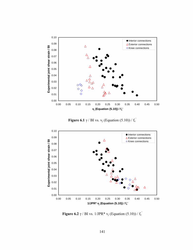
141

0.00

0.01

0.02

0.03

0.04

0.05

0.06

0.07

0.08

0.09

0.10

0.00 0.05 0.10 0.15 0.20 0.25 0.30 0.35 0.40 0.45 0.50

vj (Equation (5.10)) / fc'

Expe

rimen

tal j

oint

she

ar s

trai

n / B

I

Interior connectionsExterior connectionsKnee connections

Figure 6.1 γ / BI vs. vj (Equation (5.10)) / fc’

0.00

0.01

0.02

0.03

0.04

0.05

0.06

0.07

0.08

0.09

0.10

0.00 0.05 0.10 0.15 0.20 0.25 0.30 0.35 0.40 0.45 0.50

1/JPR* vj (Equation (5.10)) / fc'

Expe

rimen

tal j

oint

she

ar s

trai

n / B

I

Interior connectionsExterior connectionsKnee connections

Figure 6.2 γ / BI vs. 1/JPR* vj (Equation (5.10)) / fc’

142

0.000

0.005

0.010

0.015

0.020

0.025

0.030

0.035

0.040

0.000 0.005 0.010 0.015 0.020 0.025 0.030 0.035 0.040

Joint shear deformation model (Equation (6.2), Rad)

Expe

rimen

tal j

oint

she

ar d

efor

mat

ion

(Rad

)

Figure 6.3 Experimental joint shear deformation vs. Equation (6.2)

0.000

0.005

0.010

0.015

0.020

0.025

0.030

0.035

0.040

0.000 0.005 0.010 0.015 0.020 0.025 0.030 0.035 0.040

Joint shear deformation model (Equation (6.4), Rad)

Expe

rimen

tal j

oint

she

ar s

trai

n (R

ad)

Figure 6.4 Experimental joint shear deformation vs. Equation (6.4)

143

0.00

0.02

0.04

0.06

0.08

0.10

0.12

0.14

0.16

0.18

0.20

0.00 0.05 0.10 0.15 0.20 0.25 0.30 0.35 0.40 0.45

vj (Equation (5.17)) / fc'

Expe

rimen

tal j

oint

she

ar d

efor

mat

ion

/ BI

Subassemblies with below 0.70 in Ash ratio

Subassemblies with equal to or above 0.70 in Ash ratio

Figure 6.5 γ / BI vs. vj (Equation 5.17) / fc’ (Interior connections)

0.000

0.005

0.010

0.015

0.020

0.025

0.030

0.035

0.040

0.045

0.050

0.000 0.010 0.020 0.030 0.040 0.050

Joint Shear deformation model (Equation (6.9), Rad)

Expe

rimen

tal j

oint

she

ar d

efor

mat

ion

(Rad

)

Figure 6.6 Experimental joint shear deformation vs. Equation (6.9)

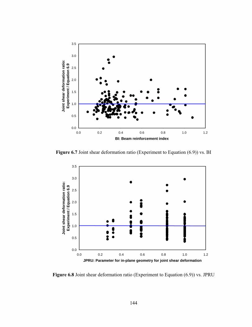
144

0.0

0.5

1.0

1.5

2.0

2.5

3.0

3.5

0.0 0.2 0.4 0.6 0.8 1.0 1.2

BI: Beam reinforcement index

Join

t she

ar d

efor

mat

ion

ratio

: Ex

perim

ent /

Equ

atio

n 6.

9

Figure 6.7 Joint shear deformation ratio (Experiment to Equation (6.9)) vs. BI

0.0

0.5

1.0

1.5

2.0

2.5

3.0

3.5

0.0 0.2 0.4 0.6 0.8 1.0 1.2

JPRU: Parameter for in-plane geometry for joint shear deformation

Join

t she

ar d

efor

mat

ion

ratio

: Ex

perim

ent /

Equ

atio

n 6.

9

Figure 6.8 Joint shear deformation ratio (Experiment to Equation (6.9)) vs. JPRU

145

0.0

0.5

1.0

1.5

2.0

2.5

3.0

3.5

0.00 0.10 0.20 0.30 0.40 0.50vj (Equation 5.20) / fc'

Join

t she

ar d

efor

mat

ion

ratio

: Ex

perim

ent /

Equ

atio

n 6.

9

Figure 6.9 Joint shear deformation ratio (Experiment to Equation (6.9)) vs. vj/fc’

0.0

0.5

1.0

1.5

2.0

2.5

3.0

3.5

0.9 1.0 1.1 1.2 1.3

TB: Parameter for out-of-plane members

Join

t she

ar d

efor

mat

ion

ratio

: Ex

perim

ent /

Equ

atio

n 6.

9

Figure 6.10 Joint shear deformation ratio (Experiment to Equation (6.9)) vs. TB

146

0.0

0.5

1.0

1.5

2.0

2.5

3.0

3.5

0.00 0.05 0.10 0.15 0.20 0.25 0.30

JI: Parameter for joint transverse reinforcement

Join

t she

ar d

efor

mat

ion

ratio

: Ex

perim

ent /

Equ

atio

n 6.

9

Figure 6.11 Joint shear deformation ratio (Experiment to Equation (6.9)) vs. JI

0.0

0.5

1.0

1.5

2.0

2.5

3.0

3.5

0.6 0.7 0.8 0.9 1.0 1.1

1-e/bc: Parameter for joint eccentricity

Join

t she

ar d

efor

mat

ion

ratio

: Ex

perim

ent /

Equ

atio

n 6.

9

Figure 6.12 Joint shear deformation ratio (Experiment to Equation (6.9)) vs. 1-e/bc

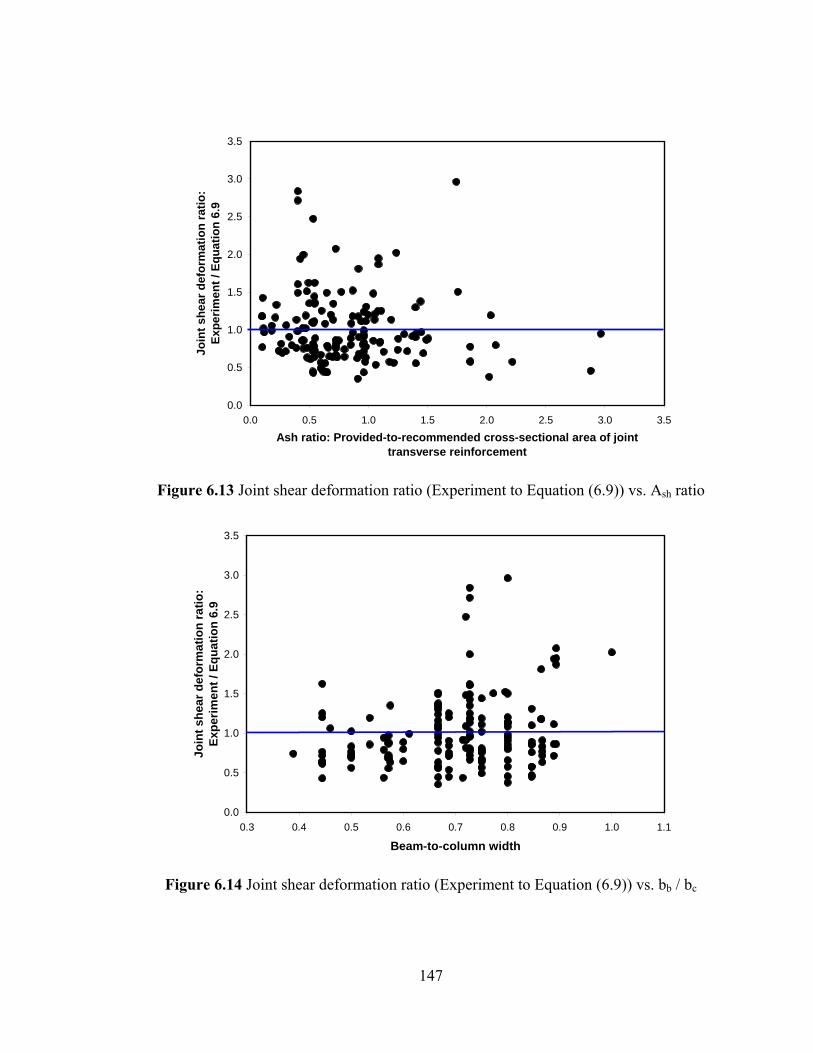
147

0.0

0.5

1.0

1.5

2.0

2.5

3.0

3.5

0.0 0.5 1.0 1.5 2.0 2.5 3.0 3.5

Ash ratio: Provided-to-recommended cross-sectional area of joint transverse reinforcement

Join

t she

ar d

efor

mat

ion

ratio

: Ex

perim

ent /

Equ

atio

n 6.

9

Figure 6.13 Joint shear deformation ratio (Experiment to Equation (6.9)) vs. Ash ratio

0.0

0.5

1.0

1.5

2.0

2.5

3.0

3.5

0.3 0.4 0.5 0.6 0.7 0.8 0.9 1.0 1.1

Beam-to-column width

Join

t she

ar d

efor

mat

ion

ratio

: Ex

perim

ent /

Equ

atio

n 6.

9

Figure 6.14 Joint shear deformation ratio (Experiment to Equation (6.9)) vs. bb / bc

148

0.0

0.5

1.0

1.5

2.0

2.5

3.0

3.5

0.0 0.5 1.0 1.5 2.0 2.5

Spacing ratio: Provided-to-recommended spacing of joint transverse reinforcement

Join

t she

ar d

efor

mat

ion

ratio

: Ex

perim

ent /

Equ

atio

n 6.

9

Figure 6.15 Joint shear deformation ratio (Experiment to Equation (6.9)) vs. Spacing ratio

0.0

0.5

1.0

1.5

2.0

2.5

3.0

3.5

0.8 1.0 1.2 1.4 1.6 1.8 2.0 2.2 2.4

Beam height to column depth

Join

t she

ar d

efor

mat

ion

ratio

: Ex

perim

ent /

Equ

atio

n 6.

9

Figure 6.16 Joint shear deformation ratio (Experiment to Equation (6.9)) vs. hb /hc

149

0

5

10

15

20

25

30

0 5 10 15 20 25 30

Joint shear model (point B, Equation (6.13), MPa)

Expe

rimen

tal j

oint

she

ar s

tres

s (M

Pa)

Figure 6.17 Experimental joint shear stress at point B vs. Equation (6.13)

0.000

0.005

0.010

0.015

0.020

0.000 0.005 0.010 0.015 0.020

Joint shear strain model (point B, Equation (6.17), Rad)

Expe

rimen

tal j

oint

she

ar s

trai

n (p

oint

B, R

ad)

Figure 6.18 Experimental joint shear strain at point B vs. Equation (6.17)

150

0

5

10

15

20

0 5 10 15 20

Joint shear model (point A, Equation (6.20), MPa)

Expe

rimen

tal j

oint

she

ar s

tres

s (p

oint

A, M

Pa)

Figure 6.19 Experimental joint shear stress point A vs. Equation (6.20)

0.0000

0.0002

0.0004

0.0006

0.0008

0.0010

0.0000 0.0002 0.0004 0.0006 0.0008 0.0010Joint shear strain model (point A, Equation (6.23), Rad)

Expe

rimen

tal j

oint

she

ar s

trai

n (p

oint

A, R

ad)

Figure 6.20 Experimental joint shear strain point A vs. Equation (6.23)

151

0.3

0.4

0.5

0.6

0.7

0.8

0.9

1.0

1.1

0 20 40 60 80 100 120Number of data

v j (t

he lo

wes

t poi

nt p

rovi

ded

in p

aper

) / v

j (m

axim

um)

Average=0.84

If point D (descending) is determined as 90% of maximum, 72% cases are available 85% of maximum, 53% cases are available 80% of maximum, 33% cases are available 75% of maximum, 18% cases are available 70% of maximum, 6% cases are available

Figure 6.21 Joint shear stress ratio vs. Number of data

0.00

0.01

0.02

0.03

0.04

0.05

0.06

0.07

0.08

0.09

0.10

0.00 0.01 0.02 0.03 0.04 0.05 0.06 0.07 0.08 0.09 0.10Joint shear strain (point D, Equation (6.29), Rad)

Expe

rimen

tal j

oint

she

ar s

trai

n (p

oint

D, R

ad)

Figure 6.22 Joint shear strain at point D. vs. Equation (6.29)

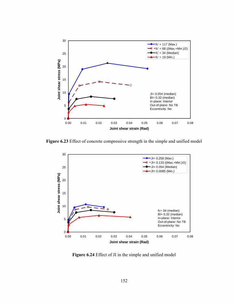
152

0

5

10

15

20

25

30

0.00 0.01 0.02 0.03 0.04 0.05 0.06 0.07 0.08

Joint shear strain (Rad)

Join

t she

ar s

tres

s (M

Pa)

fc' = 117 (Max.)fc' = 68 ((Max.+Min.)/2)fc' = 34 (Median)fc' = 19 (Min.)

JI= 0.054 (median)BI= 0.32 (median)In-plane: InteriorOut-of-plane: No TBEccentricity: No

Figure 6.23 Effect of concrete compressive strength in the simple and unified model

0

5

10

15

20

25

30

0.00 0.01 0.02 0.03 0.04 0.05 0.06 0.07 0.08

Joint shear strain (Rad)

Join

t she

ar s

tres

s (M

Pa)

JI= 0.258 (Max.)JI= 0.133 ((Max.+Min.)/2)JI= 0.054 (Median)JI= 0.0085 (Min.)

fc= 34 (median)BI= 0.32 (median)In-plane: InteriorOut-of-plane: No TBEccentricity: No

Figure 6.24 Effect of JI in the simple and unified model

153

0

5

10

15

20

25

30

0.00 0.01 0.02 0.03 0.04 0.05 0.06 0.07 0.08

Joint shear strain (Rad)

Join

t she

ar s

tres

s (M

Pa)

BI= 1.078 (Max.)BI= 0.580 ((Max.+Min.)/2)BI= 0.320 (Median)BI= 0.087 (Min.)

fc= 34 (median)JI= 0.054 (median)In-plane: InteriorOut-of-plane: No TBEccentricity: No

Figure 6.25 Effect of BI in the simple and unified model

0

5

10

15

20

25

30

0.00 0.01 0.02 0.03 0.04 0.05 0.06 0.07 0.08

Joint shear strain (Rad)

Join

t she

ar s

tres

s (M

Pa)

1-e/bc=1.0 (max)1-e/bc=0.79 (median)1-e/bc=0.69 (min)

JI= 0.054 (median)BI= 0.32 (median)fc= 34 (median)In-plane: InteriorOut-of-plane: No TB

Figure 6.26 Effect of degree of joint eccentricity in the simple and unified model

154

0

5

10

15

20

25

30

0.00 0.01 0.02 0.03 0.04 0.05 0.06 0.07 0.08

Joint shear strain (Rad)

Join

t she

ar s

tres

s (M

Pa)

InteriorExteriorKnee

JI= 0.054 (median)BI= 0.32 (median)fc= 34 (median)Out-of-plane: No TBEccentricity: No

Figure 6.27 Effect of in-plane geometry in the simple and unified model

0

5

10

15

20

25

30

0.00 0.01 0.02 0.03 0.04 0.05 0.06 0.07 0.08

Joint shear strain (Rad)

Join

t she

ar s

tres

s (M

Pa)

2 transverse beams1transverse beam0 transverse beam

JI= 0.054 (median)BI= 0.32 (median)fc= 34 (median)In-plane: InteriorEccentricity: No

Figure 6.28 Effect of out-of-plane geometry in the simple and unified model

155

0

5

10

15

20

25

30

0.00 0.01 0.02 0.03 0.04 0.05

Joint shear strain (Rad)

Join

t she

ar s

tres

s (M

Pa)

ExperimentSimple and unified modelFEMA 356Teraoka and FujiiParra-Montesinos and WightModified Parra-Montesinos and Wight modelMCFT

Noguchi: OKJ 1 (Interior)

Figure 6.29 Comparison RC joint shear behavior (OKJ1 tested by Noguchi and Kashiwazaki (1992))

156

Figure 6.30 FEMA 356 generic joint shear behavior model

A

B C

D

E

ab

cJoin

t she

ar s

tres

s

Joint shear strain

Figure 6.31 Adjusted FEMA 356 joint shear behavior model

157

0

5

10

15

20

25

30

0 5 10 15 20 25 30

Joint shear model (FEMA 356 or Equation (5.21), MPa)

Expe

rimen

tal j

oint

she

ar s

tres

s (M

Pa)

FEMA 356

Equation 5.21

Figure 6.32 Comparison of FEMA 356 and Equation (5.21)

0.000

0.005

0.010

0.015

0.020

0.025

0.030

0.035

0.040

0.000 0.005 0.010 0.015 0.020 0.025 0.030 0.035 0.040

Joint shear strain "a" from FEMA 356 or developed model

Expe

rimen

tal j

oint

she

ar s

trai

n "a

"

Developed model (Table 6.18)

FEMA 356

Figure 6.33 Comparison of FEMA 356 and Developed model

158

0

5

10

15

20

25

30

0 5 10 15 20 25 30

Equation (5.21) or Teraoka and Fujii model (MPa)

Expe

rimen

tal j

oint

she

ar s

tres

s (M

Pa)

Teraoka and Fujii (equal to or above 0.70 in Ash ratio)Teraoka and Fujii (below 0.70 in Ash ratio)Equation (5.21)

Figure 6.34 Comparison of Teraoka and Fujii and Equation (5.21) for point C stress

0.00

0.01

0.02

0.03

0.04

0.05

0.00 0.01 0.02 0.03 0.04 0.05

Equation (6.9) or Teraoka and Fujii model (Rad)

Expe

rimen

tal j

oint

she

ar s

trai

n (R

ad)

Teraoka and Fujii (Equal to or above 0.70 in Ash ratio)Teraoka and Fujii (Below 0.70 in Ash ratio)Equation (6.9)

Figure 6.35 Comparison of Teraoka and Fujii and Equation (6.9) for point C strain

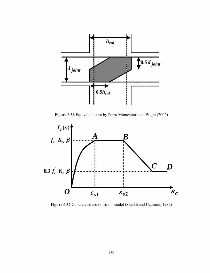
159

colh

colh5.0

ntjoid5.0ntjoid

Figure 6.36 Equivalent strut by Parra-Montesinos and Wight (2002)

)(εcf

βsc Kf '

βsc Kf '3.0

2sε1sε cεO

A B

C D

Figure 6.37 Concrete stress vs. strain model (Sheikh and Uzumeri, 1982)

160

0

5

10

15

20

25

30

0 5 10 15 20 25 30

Joint shear stress (point C, Equation (5.21) or PW model, MPa)

Expe

rimen

tal j

oint

she

ar s

tres

s (p

oint

C, M

Pa)

Parra-Montesinos and WightEquation 5.21

Figure 6.38 Comparison of Parra-Montesinos and Wight model and Equation (5.21) for point C stress

0.00

0.01

0.02

0.03

0.04

0.05

0.00 0.01 0.02 0.03 0.04 0.05

Joint shear strain (point C, Equation (6.9) or PW model, Rad)

Expe

rimen

tal j

oint

she

ar s

trai

n (p

oint

C, R

ad)

Parra-Montesinos and WightEquation (6.9)

Figure 6.39 Comparison of Parra-Montesinos and Wight model and Equation (6.9) for point C strain

161

0

5

10

15

20

25

30

0 5 10 15 20 25 30

Joint shear stress (point C, Equation (5.21) or MCFT, MPa)

Expe

rimen

tal j

oint

she

ar s

tres

s (p

oint

C, M

Pa)

MCFTEquation 5.21

Figure 6.40 Comparison of MCFT and Equation (5.21) for point C stress

0.000

0.010

0.020

0.030

0.040

0.050

0.000 0.010 0.020 0.030 0.040 0.050

Joint shear strain (point C, Equation (6.9) or MCFT, Rad)

Expe

rimen

tal j

oint

she

ar s

trai

n (p

oint

C, R

ad)

MCFTEquation 6.9

Figure 6.41 Comparison of MCFT and Equation (6.9) for point C strain

162

0

1

2

3

4

5

6

7

8

9

10

0.000 0.005 0.010 0.015 0.020 0.025 0.030 0.035 0.040

Experimental joint shear strain (Rad)

Com

pute

d pr

inci

pal s

trai

n ra

tio

(tens

ile /

com

pres

sive

)

Noguchi: OKJ 5In-plane geometry: InteriorOut-of-plane geometry: No transverse beam and slabJoint eccentricity: No

A

B

C

D

Figure 6.42 Computed principal strain ratio at a given joint shear strain (Noguchi OKJ 3)

B

C

γ

tcK

i,tcK

s,tcK

Figure 6.43 Simplified principal strain ratio vs. joint shear strain

163

0

5

10

15

20

25

30

0 5 10 15 20 25 30

Joint shear stress (Modified PW model or Equation (5.21), MPa)

Expe

rimen

tal j

oint

she

ar s

tres

s (M

Pa)

Modified Parra-Montesinos and Wight model

Equation 5.21

Figure 6.44 Comparison of updated Parra-Montesinos and Wight model and Equation (5.21) for point C stress

0.000

0.005

0.010

0.015

0.020

0.025

0.030

0.035

0.040

0.045

0.050

0.000 0.005 0.010 0.015 0.020 0.025 0.030 0.035 0.040 0.045 0.050Joint shear strain (Modified PW model or Equation (6.9), Rad)

Expe

rimen

tal j

oint

she

ar s

trai

n (R

ad)

Modified Parra-Montesinos and Wight model

Equation 6.9

Figure 6.45 Comparison of updated Parra-Montesinos and Wight model and Equation (6.9) for point C strain

164

Chapter 7

CONCLUSIONS AND RECOMMENDATIONS

7.1 Conclusions

The overall objective of this research has been to provide a more profound understanding of joint shear structural behavior for diverse types of RC beam-column connections subjected to seismic lateral loading. This initiative has been accomplished by construction of a thorough database of experiments, characterization of RC joint shear behavior, development of RC joint shear strength models, and proposals for complete RC joint shear behavior models. The key findings and recommendations of this research are generally applicable to RC beam-column connections that have conditions similar to those of the constructed database. For each task, important findings and conclusions are summarized as follows.

7.1.1 Construction of experimental database

The experimental database was constructed by employing inclusion criteria and classifying RC beam-column connection subassemblies according to factors they have in common. Then, the minimum amount of joint transverse reinforcement to maintain proper joint confinement was determined. Finally, the ACI 352R-02 joint shear strength definition was briefly examined.

Inclusion criteria: All included subassemblies were laboratory tests subjected to quasi-static cyclic lateral loading and their scales were at least one-third (usually equal to or above half scale). All subassemblies in the database had joint shear failure, either in conjunction with or without yielding of longitudinal beam reinforcement, as their governing failure mode. Finally, the constructed database only included subassemblies with conventional types of reinforcement anchorage, in which the longitudinal beam and column reinforcement are either anchored by standard hooks or pass through the joint panel (as dictated by in-plane geometry). During the collected experimental test results, 341 subassemblies satisfied these inclusion criteria and were therefore included in the database.

Database classification: The constructed database (341 subassemblies in total) was classified according to in-plane geometry (interior, exterior, and knee joints), out-of-plane geometry (number of transverse beams), joint eccentricity, and governing failure mode sequence. Within the constructed database, 261 subassemblies had no out-of-plane members and no joint eccentricity (148 interior, 95 exterior, and 18 knee joints), 36 subassemblies had out-of-plane members (transverse beam(s) and/or slab(s)) and no joint eccentricity (30 interior and 6 exterior joints), 26 specimens had eccentricity with or without out-of-plane members, and 18 subassemblies had no joint transverse reinforcement.

165

Minimum amount of joint transverse reinforcement: The strain condition of joint transverse reinforcement was checked from experimental tests governed by beam flexural failure and without out-of-plane members; it remained in the elastic range during experimental testing when the shA ratio equal to or above 0.70. (Examination of the role of the ACI 352R-02 design guidelines with respect to joint shear strength also confirmed that a reduction in joint shear strength due to insufficient joint transverse reinforcement could be effectively prevented when the shA ratio is equal to or above 0.70.)

ACI 352R-02 joint shear strength definition: The reduced dataset (subassemblies with shA ratio equal to or above 0.70) was used for an examination of the ACI 352R-02 joint

shear strength definition. The fraction of experimental cases that had lower normalized experimental RC joint shear strength than predicted by ACI 352R-02 were 6%, 44%, and 40% for interior, exterior, and knee connections, respectively. The current ACI 352R-02 definition appears to result in a wide scatter in determining joint shear strength and to not evenly consider the effect of geometry on joint shear strength.

7.1.2 Characterization of joint shear behavior

RC joint shear behavior was characterized by identifying key points (displaying distinct stiffness changes), by introducing possible material and geometric influence parameters, and by assessing the affect of these parameters. The effects of insufficient joint confinement, out-of-plane geometry, and joint eccentricity in joint shear behavior were also examined.

Key points of joint shear behavior: Joint shear stress vs. joint shear strain can be represented as a schematic envelope curve by connecting key points that exhibit distinct changes in stiffness. The first key point (point A) indicates diagonal cracking within a joint panel, the second key point (point B) results from yielding of (joint transverse or longitudinal beam) reinforcement, and the third key point (point C) corresponds to the maximum response. Within the constructed database, experimental test results showed that the points displaying the most distinctive stiffness changes are similar in both overall (subassembly) and local (joint) behavior.

Determination of examined parameters: Based on careful literature review, concrete compressive strength, in-plane geometry, out-of-plane geometry, joint eccentricity, beam width to column width ratio, beam height to column depth ratio, joint transverse reinforcement index, beam reinforcement index, column reinforcement index, column axial stress to concrete compressive strength ratio, and bond demand levels were selected to describe diverse conditions of RC beam-column connections.

Joint shear stress and strain at cracking: The RC joint shear stress/strain relationship was derived by stress/strain coordinate transformation, and these derived equations could roughly predict joint shear stress/strain at point A (displaying the first distinct stiffness change).

Influence parameters for basic dataset: Points B and C were examined to assess the effect of the various influence parameters on joint shear behavior by using the basic

166

dataset (subassemblies with equal to or above 0.70 in shA ratio, no out-of-plane members, and no joint eccentricity). Concrete compressive strength is the strongest influence parameter, and in-plane geometry is also important in determining joint shear capacity. Improved joint shear force resistance generally triggers a stiffer response in joint shear behavior. Joint transverse reinforcement does not significantly affect joint shear capacity because the selected subassemblies maintain proper joint confinement. The role of beam reinforcement is not distinctive when failure modes are separated into “BJ” and “J”. Joint shear behavior is little influenced by the beam width to column width, beam height to column depth, or column axial stress to concrete compressive strength ratios.

Insufficient joint confinement: Insufficient joint confinement (caused by an inadequate amount of joint transverse reinforcement) does not change the key influence parameters on joint shear behavior; however, it somewhat attenuates the relation between joint shear stress (or strain) and the key influence parameters. In addition, the role of joint transverse reinforcement appears more distinctive after considering experimental tests with insufficient joint confinement.

Out-of-plane geometry: Initiation of joint shear failure results in the excessive expansion of the joint panel in both the in-plane and out-of-plane directions, and passive confinement to the joint panel can be activated from the longitudinal reinforcement of transverse beams. Only the presence of two transverse beams is beneficial for the improvement of joint shear capacity.

Joint eccentricity: The generated torsion due to the eccentricity between the centerline of the longitudinal beam and the centerline of the column cross-section weakens the joint shear resistance mechanism. Joint eccentricity also results in a reduction in joint shear stiffness.

7.1.3 Development of joint shear strength models

Key findings and conclusions related to the development of the RC joint shear strength models may be summarized as follows:

Procedural framework: Without relying on a previous deterministic joint shear strength model (such as the ACI 352R-02 joint shear strength model), an RC joint shear strength model was developed using the Bayesian parameter estimation method for the basic dataset (subassemblies with shA ratios equal to or above 0.70, no out-of-plane members, and no joint eccentricity). Based on this established procedure, the important parameters that influence RC joint shear strength were explicitly identified: concrete compressive strength, in-plane geometry, beam reinforcement, and joint transverse reinforcement are more important than the other examined parameters.

Simple and unified joint shear strength model: For the total database (except subassemblies with no joint transverse reinforcement), a unified joint shear strength model was constructed and then simplified to be applicable to practical design situations. In the final simple and unified model, RC joint shear strength is determined by

167

considering concrete compressive strength, in-plane geometry, beam reinforcement, joint transverse reinforcement, out-of-plane geometry, and joint eccentricity.

Performance evaluation (RC joint shear strength): The performance of the joint shear strength models (Equation (5.16) and other deterministic models) was evaluated by quantifying the overall model uncertainty and visually confirmed by plotting the joint shear stress ratio (experimental joint shear stress to joint shear stress defined by a particular deterministic model) vs. concrete compressive strength. ACI 352R-02, ACI 318-05, AIJ 1999, and NZS 3101:1995 are biased in the conservative direction. The simple and unified model shows the smallest level of model uncertainty compared to code definitions. Among the code definitions, AIJ 1999 causes the least scatter in determining RC joint shear strength, which means that a value of around 0.75 for the power term of concrete compressive strength (the governing parameter) can reduce model uncertainty significantly. In addition, the suggested model (Equation (5.16)) is also more reliable in determining RC joint shear strength than the proposed models by Murakami et al. (only for interior connections) and Russo and Somma (only for exterior connections).

Anchorage plates and fiber-reinforced concrete: The location of the anchorage plate, when used for longitudinal beam reinforcement, affects joint shear strength. The RC joint shear strengths for subassemblies that had anchorage plates located within the joint core were similar to those for subassemblies with general 90-degree hook. Additionally, using fiber-reinforced concrete within the joint panel is beneficial in improving RC joint shear capacity compared to normal concrete within the joint panel.

Modification of ACI 352R-02 joint shear strength: Another unbiased RC joint shear strength model was developed by fixing the contribution of concrete compressive strength and then only considering the parameters that are currently included in the ACI 352R-02 joint shear strength definition. The quantified model uncertainty indicates that a more reliable joint shear strength model can be constructed following the current general ACI 352R-02 approach. This modified model more effectively accounts for the change of joint shear strength according to geometry compared to the current ACI 352R-02 joint shear strength model.

7.1.4 Complete joint shear stress vs. strain prediction model

Key findings and conclusions related to modeling the complete RC joint shear behavior (joint shear stress vs. strain) are as follows:

Joint shear deformation model (at maximum response): An RC joint shear deformation model was first constructed by the Bayesian parameter estimation method for the basic dataset, and it was continuously updated until using the total database (except for subassemblies with no joint transverse reinforcement). Finally, a unified joint shear deformation model was constructed for the total database and was simplified to be applicable to practical situations. (To the knowledge of the author, there has been no broadly applicable suggested and accepted RC joint shear deformation modeling before this research.) In the final simple and unified joint shear deformation model, the joint

168

shear strength model to concrete compressive strength ratio, in-plane geometry, beam reinforcement, joint transverse reinforcement, out-of-plane geometry, and joint eccentricity were included. Therefore, the surviving parameters are similar in both the simple and unified joint shear strength and deformation models.

Joint shear behavior prediction model: RC joint shear behavior models were constructed by the Bayesian method at each key point (cracking, reinforcement yielding, maximum, and descending) and also by simply adjusting the simple and unified joint shear strength and deformation models proposed for maximum response. The RC joint shear behavior model proposed by adjusting the simple and unified joint shear strength and deformation models (the simple and unified joint shear behavior model) is recommended because this approach is simple, lending itself to practical situations, and also because it does not cause significant reduction in model reliability compared to the model constructed by the Bayesian method for each key point.

Parameter effects in the simple and unified RC joint shear behavior model: An increase of concrete compressive strength, beam reinforcement, in-plane geometry, and out-of-plane geometry result in an increase in both joint shear stress and strain at key points. An increase of joint transverse reinforcement triggers an improvement in joint shear stiffness (increase in stress and decrease in strain). On the other hand, joint eccentricity causes a reduction in joint shear stiffness (decrease in stress and increase in strain).

Performance evaluation (overall joint shear behavior): For visual comparison, the RC joint shear stress vs. joint shear strain behaviors were plotted following the FEMA 356 model, the Teraoka and Fujii model, the Parra-Montesinos and Wight model, the MCFT, and the simple and unified joint shear behavior model. Then, for each behavior model, model uncertainty was quantified at maximum response (for both stress and deformation). When considering the visual comparison and quantified model uncertainty, the simple and unified joint shear behavior model is the best in determining the RC joint shear behavior for diverse types of RC beam-column connections, in spite of its greater simplicity. In general, many of the other models result in descriptions of joint shear behavior that is biased in a conservative direction.

Modified Parra-Montesinos and Wight model: The Parra-Montesinos and Wight model was modified to improve its performance with respect to predicted joint shear behavior because their approach could be employed across most of the constructed database. In this modification, the key relation between principal strain ratio (principal tensile strain to principal compressive strain) and joint shear strain was suggested as the combination of an initial principal strain ratio and a principal strain ratio slope. This modified Parra-Montesinos and Wight model provides a significantly reduced value of model uncertainty compared to the original Parra-Montesinos and Wight model, and its performance is the best of all the examined joint shear behavior models except for the developed simple and unified joint shear behavior model.

169

7.2 Recommendations for future research

Several interesting “new” questions (related to this current work) arose during performing the research described herein. The following topics can be recommended as subjects for future research study.

• The developed model in this research suggests an envelope curve for RC joint shear stress vs. strain behavior. To employ this suggested envelope model in the analysis of RC beam-column connections subjected to cyclic or dynamic loading (rather than only in pushover analyses), additional definitions about unloading, reloading, and damage are needed to describe strength and energy degradation due to repeated cyclic loading.

• An RC beam-column connection subassembly consists of beam(s), a column, and a joint panel. In modeling an RC beam-column connection subassembly, beam plastic behavior and joint shear behavior have not been nearly as well-established as compared to the (cracked) linear behavior of the beam and column members. Because the suggested joint shear behavior model can be used in the modeling of pushover tests of RC beam-column connections (and frames), the development of an appropriate beam plastic model could provide for a more established overall analytical procedure (though some existing models may be available in the literature).

• The suggested joint shear behavior model was constructed based on standard experimental tests of RC beam-column connection subassemblies. Because the boundary conditions of RC beam-column connections are often different in real RC moment resisting frames (MRF), the effect of boundary conditions on joint shear behavior could be further investigated.

• Based on experimental observations, fragility curves may be required to decide damage states, an appropriate repair method, and/or the failure probability according to various demand parameters (such as overall story drift). These fragility curves (which could be developed in part from the assembled database) can improve understanding of the vulnerability of RC beam-column connections subjected to earthquake loading.

• More experimental tests for RC beam-column connections with specific conditions such as using headed bars or fiber reinforced concrete will be beneficial in the extension of understanding behavior of RC beam-column connections.

170

References

Abrams, D. P., (1987), “Scale relations for reinforced concrete beam-column joints,” ACI Structural Journal, 84(6), 502-512.

ACI-ASCE Committee 352 (2002), “Recommendations for design of beam-column joints in monolithic reinforced concrete structures (ACI 352R-02),” American Concrete Institute, Farmington Hills, MI

ACI Committee 318 (2005), “Building code requirements for reinforced concrete (ACI 318-05) and commentary (ACI 318R-05),” American Concrete Institute, Farmington Hills, MI

Alameddine, F. and Ehsani, M. R., (1989), “Seismic design recommendations for high-strength concrete beam-to-column connections,” Report No. CEEM-89-105, University of Arizona, Tucson, AZ

Ang A. H-S. and Tang W. H., (1975), “Probability concepts in engineering planning and design, volume I-basic principles,” John Wiley & Sons, Inc., 605 Third Avenue New York, NY

Aota, K., Watanabe, T., Naruse, T., and Morimoto, T., (2001), “Anchorage method using end plate of top story beam-column connections (in Japanese),” Proceedings of the Japan Concrete Institute, 23(3), 391-396.

Architectural Institute of Japan, (1999), “Design guideline for earthquake resistance reinforced concrete buildings based on inelastic displacement concept,” Tokyo, Japan

Asou, N., Nagashima, T., and Sugano, S., (1993) “Force characteristic of beam column connection using high strength concrete (Fc600) and reinforcement (SD490) (in Japanese),” Proceedings of the Japan Concrete Institute, 15(2), 553-558.

Attaalla, S. A., (2004), “General analytical model for normal shear stress of type 2 normal and high strength concrete beam-column joints,” ACI Structural Journal, 101(1), 65-75.

Bayasi, Z. and Gebman, M., (2002), “Reduction of lateral reinforcement in seismic beam-column connection via application of steel fibers,” ACI Structural Journal, 99(6), 772-780.

Bentz, E. and Collins, M. P., (2001), “2D Sectional analysis of membranes (Membrane-2000)”, University of Toronto, Canada.

Bonacci, J. and Pantazopoulou, S., (1993), “Parametric investigation of joint mechanics,” ACI Structural Journal, 90(1), 61-70.

Box, G. E. P. and Tiao, G. C., (1992), “Bayesian inference in statistical analysis,”

171

Addison-Wesley, Reading, MA

Briss, G. R., (1978), “The elastic behavior of earthquake-resistant reinforced concrete beam-column joints,” Report No 78-13, Department of Civil Engineering, University of Canterbury, Christchurch, New Zealand

Chang, K. W., Kim, Y. I., and Oh, Y. H., (1997), “Slab effect on inelastic behavior of high strength RC beam-column joints (in Korean),” Journal of the Korean Concrete Institute, 9(2), 167-177.

Chen, W. F. and Saleeb, A. F., (1994), “Constitutive equations for engineering materials Volume 1: elasticity and modeling,” Elsevier, NY, 259.

Choi, G., Fujii, S., and Watanabe, F., (2001), “ Influence of reinforcement arrangement on shear strength in L and T shape connection (in Japanese),” Proceedings of the Japan Concrete Institute, 23(3), 397-402.

Chun, S. C., Lee, S. H., Kang, T. H.-K., Oh, B., and Wallace, J.W., (2007), “Mechanical anchorage in exterior beam-column joints subjected to cyclic loading,” ACI Structural Journal, 104(1), 102-112.

Chutarat, N. and Aboutaha, R. S., (2003), “Cyclic response of exterior reinforced concrete beam-column joints reinforced with headed bars-experimental investigation,” ACI Structural Journal, 100(2), 259-264.

Cote, P. A. and Wallace, J. W., (1994), “A study of RC knee-joints subjected to cyclic lateral loading,” Report No. CU/CEE-94/04, Department of Civil and Environmental Engineering, Clarkson University, Postdam, NY

Craig, R. J., Mahadev, S., Patel, C. C., Viteri, M., and Kertesz, C., (1984), “Behavior of joints using reinforced fibrous concrete,” Fiber Reinforced Concrete (SP 81), American Concrete Institute, Detroit, MI, 125-167.

Durrani, A. J. and Wight, J. K. (1985), “Behavior of interior beam-to-column connections under earthquake-type loading,” ACI Journal, 82(3), 343-349.

Durrani, A. M. and Zerbe, H. E., (1987), “Seismic resistance of R/C exterior connections with floor slab,” Journal of Structural Engineering, ASCE, 113(8), 1850-1864.

Durrani, A. J. and Wight, J. K., (1987), “Earthquake resistance of reinforced concrete interior connections including a floor slab,” ACI Structural Journal, 84(5), 400-406.

Ehsani, M. R and Wight, J. K., (1982), “Behavior of external reinforced concrete beam to column connections subjected to earthquake type loading,” Report No. UMEE 82R5, Department of Civil Engineering, University of Michigan, Ann Arbor, MICH

172

Ehsani, M. R. and Wight, J. K., (1985), “Effect of transverse beams and slab on behavior of reinforced concrete beam-to-column connections,” ACI Journal, 82(2), 188-195.

Ehsani, M. R., Moussa, A. E., and Vallenilla, C. R., (1987), “Comparison of inelastic behavior of reinforced ordinary-and high strength concrete frames,” ACI Structural Journal, 84(2), 161-169.

Ehsani, M. R. and Alameddine, F., (1991), “Design recommendations for type 2 high-strength reinforced concrete connections,” ACI Structural Journal, 88(3), 277-291.

Ehsani, M. R. and Alameddine, F., (1991), “High-strength RC connections subjected to inelastic cyclic loading,” Journal of Structural Engineering, ASCE, 117(3), 829-850.

Endoh, Y., Kamura, T., Otani, S., and Aoyama, H., (1991), “Behavior of R/C beam-column connections using light-weight concrete,” Transactions of the Japan Concrete Institute, 13, 319-326.

Etoh, K., Kitayama, K., Tsubosaki, H., and Miyakomatsuri, H. (1991), “Recovery characteristic of RC beam column connection subjected to bi-axial loading (in Japanese),” Proceedings of the Japan Concrete Institute, 12(2), 519-524.

Federal Emergency Management Agency, (1997), “NEHRP commentary on the guidelines for the seismic rehabilitation of building (FEMA 274),” Reston, VA

Federal Emergency Management Agency, (2000), “Prestandard and commentary for the seismic rehabilitation of building (FEMA 356),” Reston, VA

Filiatrault, A., Ladicani, K., and Massicotte, B., (1994), “Seismic performance of code-designed fiber reinforced concrete joints,” ACI Structural Journal, 91(5), 564-570.

Filiatrault, A., Pineau, S., Houde, J., (1995), “Seismic behavior of steel-fiber reinforced concrete interior beam-column joints,” ACI Structural Journal, 92(5), 1-10.

Fujii, S. and Morita, S., (1991), “Comparison between interior and exterior RC beam-column joint behavior,” Design of Beam-Column Joints for Seismic Resistance (SP123), American Concrete Institute, Detroit, MI, 145-165.

Fujii, S. and Morita, S., (1987), “Behavior of exterior beam column connection under biaxial loading (in Japanese),” Proceedings of the Japan Concrete Institute, 9(2), 181-186.

Fukazawa, K., Nakano, K., Matsui, K., and Yoshimura, T., (1994), “Experimental investigation of RC column-beam joints under the influence of biaxial moments,” Transactions of the Japan Concrete Institute, 16, 491-498.

Gardoni, P., Kiureghian, A. D., and Mosalam, K. M., (2002), “Probabilistic capacity

173

models and fragility estimates for reinforced concrete columns based on experimental observations,” Journal of Engineering Mechanics, ASCE, 128(10), 1024-1038.

Gavrilovic, P., Velkov, M., Jirikovski, D., and Mamucevski, D., (1980), “Behavior of reinforced concrete beam-column joints under cyclic loading,” 7th World Conference on Earthquake Engineering, Istanbul, Turkey, 289-296.

Gefken, P. R. and Ramey, M. R., (1989), “Increased joint hoop spacing in type 2 seismic joints using fiber reinforced concrete,” ACI Structural Journal, 86(2), 168-172.

Giberson, M. F., (1969), “Two nonlinear beams with definitions of ductility,” Journal of the Structural Division, ASCE, 95(ST2), 137-157.

Ghobara, A. and Biddah, A., (1999), “Dynamic analysis of reinforced concrete frames including joint shear deformation,” Engineering Structures, 21, 971-987.

Goto, Y., Joh, O., and Shibata, T., (1992), “Influence of connection reinforcement to maximum capacity and deformation performance of RC frame (in Japanese),” Proceedings of the Japan Concrete Institute, 12(2), 401-404.

Goto, Y, and Joh, O., (1996), “An experimental study of shear failure mechanism of RC interior beam-column joints,” 11th World Conference on Earthquake Engineering, Acapulco, Mexico, 1194.

Goto, Y., Joh, O., and Yoshida, H., (1999), “Characteristic of beam reinforcement bond and failure after beam reinforcement yielding in interior RC beam column connection (in Japanese),” Proceedings of the Japan Concrete Institute, 21(3), 655-660.

Goto, Y. and Joh, O., (2003), “Experimental study on shear resistance of RC interior eccentric beam-column joints,” 9th East Asia-Pacific Conference on Structural Engineering and Construction, Bali, Indonesia, RSC-170

Goto, Y. and Joh, O., (2004), “Shear resistance of RC interior eccentric beam-column joints,” 13th World Conference on Earthquake Engineering, Vancouver, Canada, 649.

Guimaraes, G. N., Kreger, M. E., and Jirsa, J. O., (1989), “Reinforced concrete frame connections constructed using high materials,” Report, No. 89-1, Department of Civil Engineering, University of Texas at Austin, Austin, TEX

Guimaraes, G. N., Kreger, M. E., and Jirsa, J. O., (1992), “Evaluation of joint-shear provisions for interior beam-column-slab connections using high-strength materials,” ACI Structural Journal, 89(1), 89-98.

Hayashi, K., Teraoka, M., Mollick, A. A., and Kana, Y., (1993), “Bond characteristic of interior RC beam-column connections using high strength materials (in

174

Japanese),” Proceedings of the Japan Concrete Institute, 15, 1993, 583-588.

Hamada, M., Ishibashi, H., and Horie, A., (1999), “Experimental study about RC exterior beam connection (in Japanese),” Proceedings of the Japan Concrete Institute, 21(3), 667-672.

Hanson, N.W. and Connor, H.W., (1967), “Seismic resistance of reinforced concrete beam-column joints,” Journal of the Structural Division, ASCE, 93(ST5), 533-559.

Hanson, N. W., (1971), “Seismic resistance of concrete frames with grade 60 reinforcement,” Journal of the Structural Division, ASCE, 97(ST6), 1685-1700.

Hayashi, K., Kana, Y., and Teraoka, M., (1991), “Experimental study about eccentric beam column connection (in Japanese),” Proceedings of the Japan Concrete Institute, 13(2), 507-512.

Henager, C. H., (1977), “Steel fibrous, ductile concrete joint for seismic-resistant structures,” Reinforced Concrete Structures in Seismic Zones (SP53), American Concrete Institute, Detroit, MI, 371-386.

Hori, S., Iwaoka, S., Naruse, T, Yamamoto, K., Konno, S., and Watanabe, T., (2004), “Experimental study on the beam-column joints of ultra-strength reinforced concrete structures (in Japanese),” Proceedings of the Architectural Institute of Japan, Japan, 23389.

Hosono, T., Kitayama, K., Kitayama, K., Tajima, H., and Kishida, J., (2001), “Failure characteristic of RC interior beam-column connection subjected to bi-directional loading (in Japanese),” Proceedings of the Japan Concrete Institute, 23, 379-384.

Hwang, S. and Lee, H., (1999), “Analytical model for predicting shear strengths of exterior reinforced concrete beam-column joints for seismic resistance,” ACI Structural Journal, 96(5), 846-857.

Hwang, S. and Lee, H., (2000), “Analytical model for predicting shear strengths of interior reinforced concrete beam-column joints for seismic resistance,” ACI Structural Journal, 97(1), 35-44.

Hwang, S. J., Lee, H. J., Liao, T. F., Wang, K. C., and Tsai, H. H., (2005), “Role of hoops on shear strength of reinforced concrete beam-column joints,” ACI Structural Journal, 102(3), 445-453.

Inoue, H., Higashi, K., and Ohta, K., (1990), “Experimental study on effect of transverse beam and slab of reinforced cross type beam-column joints (in Japanese),” Proceedings of the Japan Concrete Institute, 12, 379-380.

Ishida, K., Fujii, S., Morita, S., and Choi, G., (1996), “Shear strength of exterior beam column connection under bi-axial earthquake loading (in Japanese),” Proceedings

175

of the Japan Concrete Institute, 18(2), 953-958.

Ishida, K., Shima, K., Higashi, K., and Fujii, S., (2001), “Real scale test of reinforced concrete + form beam-column connections (in Japanese),” Proceedings of the Japan Concrete Institute, 23, 343-348.

Ishida, K., Akiyuma, K., Pareek, S., and Kuroda, K., (2004), “Experimental study on beam-column joints of RC structures using high-strength concrete and steel (in Japanese),” Proceedings of the Architectural Institute of Japan, Japan, 779-780.

Jindal, R. L. and Hassan, K. A., (1984), “Behavior of steel fiber reinforced concrete beam-column connections,” Fiber Reinforced Concrete (SP 81), American Concrete Institute, Detroit, MI, 107-123.

Jindal, R. and Sharma, V., (1987), “Behavior of steel fiber reinforced concrete knee-type beam-column connections,” Fiber Reinforced Concrete Properties and Applications (SP 105), American Concrete Institute, Detroit, MI, 475-491.

Jiuru, T., Chaobin, H., Kaijian, Y., Yongcheng, Y., (1990), “Seismic behavior and shear strength of framed joint using steel-fiber reinforced concrete,” Journal of Structural Engineering, ASCE, 118(2), 341-357.

Joh, O., Goto, Y., and Shibata, T., (1988), “Behavior of three-dimensional reinforced concrete beam-column subassemblages with slabs,” Proceeding of 9th World Conference on Earthquake Engineering, Tokyo-Kyoto, Japan, 587-592.

Joh, O., Goto, Y, and Shibata, T., (1989), “Influence of joint reinforcement to shear resistance characteristic in RC exterior beam column connection (in Japanese),” Proceedings of the Japan Concrete Institute, 11(2), 537-542.

Joh, O., Goto, Y., and Shibata, T., (1990), “Shear resistance characteristic of exterior beam column connection using high strength concrete (in Japanese),” Proceedings of the Japan Concrete Institute, 12(2), 639-644.

Joh, O. and Goto, Y., (2000), “Beam-column joint behavior after beam yielding in R/C ductile frames,” 12th World Conference on Earthquake Engineering, New Zealand, 2196.

Joh, O., Goto, Y., and Shibata, T., (1991), “Behavior of reinforced concrete beam-column joints with eccentricity,” Design of Beam-Column Joints for Seismic Resistance (SP 123), American Concrete Institute, Detroit, MI, 317-357.

Joh, O., Goto, Y., and Shibata, T., (1992), “Shear resistance performance in RC exterior beam column connection using high strength materials (in Japanese),” Proceedings of the Japan Concrete Institute, 14(2), 391-395.

Kaku, T. and Asakusa, H., (1991), “Ductility estimation of exterior beam-column subassemblies in reinforced concrete frames,” Design of Beam-Column Joints for

176

Seismic Resistance (SP123), American Concrete Institute, Detroit, MI, 167-185.

Kaku, A., Maso, K., Kutoka, T., and Muguruma, T., (1993), “Experimental study about deformation characteristic of beam column connection in RC structure (in Japanese),” Proceedings of the Japan Concrete Institute, 15(2), 559-564.

Kamimura, T., Takeda, S., Tochio, M., (2000), “Influence of joint reinforcement on strength and deformation of interior beam-column subassemblages,” 12th World Conference on Earthquake Engineering, New Zealand, 2267

Kamimura, T., Takimoto, H., and Tanaka, S., (2004), “Mechnical behavior of reinforced concrete beam-column assemblages with eccentricity,” 13th World Conference on Earthquake Engineering, Vancouver, Canada, 4

Kaneda, K., Kondoh, G., Fujii, S., and Morita, S., (1984), “Correlation between shear failure and anchorage failure in exterior beam column connection (in Japanese),” Proceedings of the Japan Concrete Institute, 6, 665-668.

Kaneda, K., Kawabata, K., Korenaga, T., and Yasda, S. (1995), “ Bond effect on shear strength of RC beam column connection using SD 490 (in Japanese),” Proceedings of the Japan Concrete Institute, 17(2), 519-524.

Kawai, T., Kimura, H., Iwata, M., and Watai, T., (1997), “Experimental study of resistance mechanism of RC beam-column connections using high strength materials (in Japanese),” Proceedings of the Japan Concrete Institute, 19, 1011-1016.

Kawasazaki, T., Kitayama, K., and Noguchi, H., (1992), “Bond characteristic of reinforced concrete beam-column connections using ultra high strength materials (in Japanese),” Proceedings of the Japan Concrete Institute, 14, 397-400.

Kikuta S., Chiba, O., Yanagishita, K., Yamauchi, S., (1990), “Experimental study on beam-column connections using high ratio of longitudinal beam reinforcement (in Japanese),” Proceedings of the Japan Concrete Institute, 12(2), 645-650.

Kim, J. and LaFave, J. M., (2007), “Key influence parameters for the joint shear behaviour of reinforced concrete (RC) beam-column connections,” Engineering Structures, 29(10), 2523-2539.

Kim, J., LaFave, J. M., and Song, J., (2007), “A new statistical approach for joint shear strength determination of RC beam-column connections subjected to lateral earthquake loading,” Structural Engineering and Mechanics, 27(4), 439-456.

Kim, J. and LaFave J. M., (2008), “Probabilistic joint shear strength models for RC beam-column connections,” ACI Structural Journal, 105(6), 769-779.

Kitayama, K., Kurusu, K., Otani, S., and Aoyama, H., (1985), “Behavior of beam-column connections with improved beam reinforcement bond,” Transactions of the Japan

177

Concrete Institute, 7, 551-558.

Kitayama, K., Asakura, H., Otani, S., and Aoyama, H., (1988), “Earthquake resistant design criteria for reinforced concrete interior beam-column joints,” Transaction of the Japan Concrete Institute, 10, 281-288.

Kitayama, K., Kojima, C., Otani, S., and Aoyama, H., (1989), “Behavior of reinforced concrete interior beam-column connection subjected to high shear (in Japanese),” Proceedings of The Japan concrete Institute, 11(2), 531-536.

Kitayama, K., Otani, S., and Aoyama, H., (1991), “Development of design criteria for RC interior beam-column joints,” Design of Beam-Column Joints for Seismic Resistance (SP123), American Concrete Institute, Detroit, MI, 97-123.

Kitayama, K., (1992), “Restoring force characteristics in reinforced concrete beam-column joints,” Transactions of The Japan Concrete Institute, 14, 491-498.

Kitayama, K., Lee, S., Otani, S., Aoyama, H., (1992), “Behavior of high-strength R/C beam-column joints,” 10th World Conference on Earthquake Engineering, Balkma, Rotterdam, 3151-3156.

Kramer, D. A. and Shahrooz, B. M., (1994), “Seismic response of beam-column knee connections,” ACI Structural Journal, 91(3), 251-260.

Krawinkler, H. and Mohasseb, S., (1987), “Effects of panel zone deformation on seismic response,” Journal of Construction Steel Research, 8, 223-250.

Kurose, Y., (1987), “Recent studies on reinforced concrete beam-column joints in Japan,” Report, No. 87-8, Department of Civil Engineering, University of Texas at Austin, Austin, TEX

Kurose, Y., Guimaraes, G. N., Liu, Z., Kreger, M. E., and Jirsa, J. O., (1988), “Study of reinforced concrete beam-column joints under uniaxial and biaxial loading,” Report, No. 88-2, Department of Civil Engineering, University of Texas at Austin, Austin, TEX

Kurose, Y., Guimaraes, G. N., Zuhua, L., Kreger, M. E., and Jirsa, J. O., (1991), “Evaluation of slab-beam-column connections subjected to bi-directional loading,” Design of Beam-Column Joints for Seismic Resistance (SP123), American Concrete Institute, Detroit, MI, 39-67.

Kusuhara, F., Azukawa, K., Shiohara, H, and Otani, S., (2004), “Tests of reinforced concrete interior beam-column joint subassemblage with eccentric beams,” 13th World Conference on Earthquake Engineering, Vancouver, Canada, 185.

Lee, C. J. and Lee, S. H., (2000), “A study on the shear strength of reinforced concrete exterior beam-column joints (in Korean),” Journal of Architectural Institute of

178

Korea, 16(6), 21-28.

Lee, D. L., Wight, J. K., and Hanson, R. D., (1977), “RC beam-column joints under large load reversals”, Journal of the Structural Division, ASCE, 103(ST12), 2337-2350.

Lee, S., Fujita, T., Kitayama, K., and Otani, S., (1991), “Bond characteristic of beam reinforcement in RC beam-column connections using high strength material (in Japanese),” Proceedings of the Japan Concrete Institute, 13, 495-500.

Lee, S., Kitayama, K., Otani, S., and Aoyama, H., (1991), “Shear strength of interior RC beam-column connections using high strength (in Japanese),” Proceedings of the Japan Concrete Institute, 14, 379-384.

Lehman, D., Stanton, J., Anderson, M., Alire, D., and Walker, S., (2004), “Seismic performance of older beam-column joints,” 13th World Conference on Earthquake Engineering, Vancouver, Canada, 1464.

Leon, R, T., (1989), “Interior joints with variable anchorage lengths,” Journal of Structural Engineering, ASCE, 115(9), 2261-2275.

Leon, R. T., (1990), “Shear strength and hysteretic behavior of interior beam-column joints,” ACI Structural Journal, 87(1), 3-11.

Lowes, L. N. and Altoontash, A., (2003), “Modeling reinforced-concrete beam-column joints subjected to cyclic loading,” Journal of Structural Engineering, ASCE, 129(12), 1686-1697.

MacGregor, J. G., (1997), “Reinforced concrete mechanics and design,” Prentice-Hall, Upper Saddle River, NJ, 59.

Mazzoni, S., Moehle, J. P., Thewalt, C. R., (1991), “Cyclic response of RC beam-column knee joints,” Report No. UCB/EERC-91/14, College of Engineering, University of California at Berkeley, Berkeley, CAL

McConnell, S. W. and Wallace, J. W., (1994), “Use of T-headed bars in reinforced concrete knee-joints subjected to cyclic loads,” Report No. CU/CEE-94/10, Department of Civil and Environmental Engineering, Clarkson University, Psotdam, NY

McConnell, S. W. and Wallace, J. W., (1995), “Behavior of reinforced concrete beam column knee joints subjected to reversed cyclic loading,” Report No. CU/CEE-95/07, Department of Civil and Environmental Engineering, Clarkson University, Postdam, NY

Megget, L. M., (1974), “Cyclic behavior of exterior reinforced concrete beam-column joints,” Bulletin of New Zealand National Society for Earthquake Engineering, 7(1), 22-47.

179

Megget, L. M., (2003), “The seismic design and performance of reinforced concrete beam-column knee joints in building,” Earthquake Spectra, 19(4), 863-895.

Meinheit, D. F. and Jirsa, J., (1977), “The shear strength of reinforced concrete beam-column joints,” Report No 77-1, Department of Civil Engineering, University of Texas at Austin, Austin, TEX

Meinheit, D. F. and Jirsa, J., (1981), “Shear strength of R/C beam-column connections,” Journal of Structural Engineering, ASCE, 107(11), 2227-2243.

Mitra, N. and Lowes, L. N., (2007), “Evaluation, calibration, and verification of a reinforced concrete beam-column joint model”, Journal of Structural Engineering, ASCE, 133(1), 105-120.

Mitsuwa, W., Ishibashi, T., Saito, K., and Ohtsuki, S., (1992), “Experimental study about shear failure in beam column connection using high strength reinforcement (in Japanese),” Proceedings of the Japan Concrete Institute, 14(2), 385-390.

Morita, S., Kitayama, K., Koyama, A., and Hosono, T., (1999), “Effects of beam bond and column axial load on shear strength on reinforced concrete interior beam-column joints,” Transactions of the Japan Concrete Institute, 21, 453-460.

Morita, S., Kitayama, K., Kishida, S., and Nishikawa, T., (2004), “Shear force and capacity in reinforced concrete beam-column joints with good bond along beam and column bars,” 13th World Conference on Earthquake Engineering, Vancouver, Canada, 1761.

Murakami, H., Fujii, S., Ishiwata, Y., and Morita, S., (2000), “Shear strength and deformation capacity of interior R/C beam-column joint subassemblage,” 12th World Conference on Earthquake Engineering, New Zealand, 679.

Nakamura, M., Desho, S., Usami, S., and Kato, T., (1991), “Experimental study on interior beam-column join using high strength concrete and rebars (in Japanese),” Proceedings of the Architectural Institute of Japan, Japan, 21085.

Nakanish, M. and Mitsukazu, K., (1998), “Experimental study of anchorage type for reinforced concrete exterior beam-column connections,” Proceedings of the Japan Concrete Institute, 20(3), 553-558.

Nishiyama, M., Nishizaki, T., Muguruma, H., and Watanabe, F., (1989), “Seismic design of prestressed concrete beam-exterior conlumn joints,” Transactions of the Japan Concrete Institute, 11, 439-446.

Noguchi, H. and Kurusu, K., (1988), “Correlation of bond and shear in RC beam-column connections subjected to seismic forces,” 9th World Conference on Earthquake Engineering, Tokyo-Kyoto, Japan, 597-602.

Noguchi, H. and Kashiwazaki, T., (1992), “Experimental studies on shear performances

180

of RC interior column-beam joints with high-strength materials,” 10th World Conference on Earthquake Engineering, Balkma, Rotterdam, 3163-3168.

NZS 3101: part 1, (1995), “Concrete structures standard,” Standard Association of New Zealand, Willington, New Zealand

Oda, M., Kosugi, K., Yamanoka, H., and Tano, K., (1997), “Bond characteristic of longitudinal beam reinforcement in beam column connection fro high strength reinforced concrete structure (in Japanese),” Proceedings of the Japan Concrete Institute, 19(2), 993-998.

Ohnish, S. and Sugawara, M., (1990), “Experimental study about beam-column connections (in Japanese),” Proceedings of the Japan Concrete Institute, 12, 681-684.

Oh, B. G., Park, K. C., Hwang, H. S., and Chung, H. S., (1992), “An experimental study on shear capacity of reinforced concrete exterior beam-column joint with high strength concrete (in Korean),” Proceedings of the Architecture Institute of Korea, 12, 363-366.

Oka, K. and Shiohara, H. (1992), “Tests of high-strength concrete interior beam-column-joints subassemblages,” 10th World Conference on Earthquake Engineering, Balkma, Rotterdam, 3211-3217.

Ota, T., Hatato, T., Nezu, S., Sugimoto, H., Masuda, Y., Sugimoto, K., and Eto, H., (2004), “Experimental study on precise RC beam-column joint (in Japanese),” Proceedings of the Architectural Institute of Japan, Japan, 23425.

Okada, T., (1993), “Earthquake resistance of reinforced concrete structures,” University of Tokyo, Japan

Otani, S., (1974), “Inelastic analysis of R/C frame structures,” Journal of Structural Engineering, ASCE, 100(ST7), 1433-1449.

Palermo, D. and Vecchio, F. J., (2003), “Compression field modeling of reinforced concrete subjected to reversed loading: formulation,” ACI Structural Journal, 100(5), 616-625.

Parra-Montesinos, G. J., (2000), “Seismic behavior, strength, and retrofit or exterior RC column-to-steel beam connections,” Ph.D. Thesis, Department of Civil Engineering, University of Michigan, Ann Arbor, MICH

Parra-Montesinos, G. J. and Wight, J. K., (2002), “Prediction of strength and shear distortion in R/C beam-column joints,” S.M. Uzumeri Symposium - Behavior and Design of Concrete Structures for Seismic Performance (SP197), American Concrete Institute, Detroit, MI, 191-214.

Parra-Montesinos, G. J., Peterfreund, S. W., and Chao, S.-H., (2005), “Highly damage-

181

tolerant beam-column joints through use of high-performance fiber-reinforced cement composites,” ACI Structural Journal, 102(3), 487-495.

Parra-Montesinos, G. J., (2005), “High-performance fiber-reinforced cement composites: an alternative for seismic design of structures,” ACI Structural Journal, 102(5), 668-675.

Paulay, T, Park, R., and Priestley, M. J. N., (1978), “Reinforced concrete beam-column joints under seismic actions,” ACI Journal, 75(11), 585-593.

Paulay, T. and Scarpas, A., (1981), “Behavior of exterior beam-column joints,” Bulletin of New Zealand National Society for Earthquake Engineering, 14(3), 131-144.

Raffaelle, G. S., Wight, J. K., (1995), “Reinforced concrete eccentric beam-column connections subjected to earthquake-type loading,” ACI Structural Journal, 92(1), 45-55.

Russo, G. and Somma, G., (2004), “A design formula for predicting the shear strength of exterior beam column joints under seismic loading,” 13th World Conference of Earthquake Engineering, Vancouver, Canada, 1282.

Sasani, M., (2007), “Life-safety and near-collapse capacity models for seismic shear behavior of reinforced concrete columns,” ACI Structural Journal, 104(1), 30-38.

Saka, T., Otsuka, K., Yamamoto, Y., and Maruta, M., (2004), “Application of 3-D finite element analysis of reinforced concrete beam-column joint for expectation of failure mode (in Japanese),” Proceedings of the Architectural Institute of Japan, Japan, 769-770.

Sato, A. T., Yang, C., Shiohara, H., Otani, S., (2002), “Shear resisting mechanism of R/C exterior beam-column connections with post tensioned beams,” Transactions of the Japan Concrete Institute, 23, 399-406.

Sekine, M. and Ogura, K., (1983), “Experimental study of reinforced concrete exterior beam-column connections (in Japanese),” Proceedings of the Japan Concrete Institute, 5, 405-408.

Sheikh, S. A. and Uzumeri, S. M., (1982), “Analysis model for concrete confinement in tied columns,” Journal of Structural Engineering, ASCE, 108(12), 2703-2722.

Shimonoka, H, Choi, G., Uchida, T., and Fujii, S., (1997), “Shear strength of reinforced concrete T and L shape beam-column connections (in Japanese),” Proceedings of the Japan Concrete Institute, 19(2), 1023-1028.

Shin, M. and LaFave, J. M., (2004), “Modeling of cyclic joint shear deformation contributions in RC beam-column connections to overall frame behavior,” Structural Engineering and Mechanics, 18(5), 645-669.

182

Shin, M. and LaFave, J. M., (2004), “Reinforced concrete edge beam-column-slab connections subjected to earthquake loading,” Magazine of Concrete Research, 56(5), 273-291.

Shin, S. W., Lee, K. S., and Ghosh, S. K., (1992), “High-strength concrete beam-column joints,” 10th World Conference on Earthquake Engineering, Balkema, Rotterdam, 3145-3150.

Shiohara, H, Zaid, S., and Otani, S., (2001), “ Test of innovative reinforcing detail for R/C interior beam-column connections subjected to seismic action,” Proceedings of the Third International Conference on Concrete under Severe Conditions, University of British Columbia, Vancouver, Canada, 1, 739-746.

Shiohara, H., (2001), “New model for shear failure of RC interior beam-column connections,” Journal of Structural Engineering, ASCE, 127(2), 152-160.

Shiohara, H., Sato, A. T., Otani, S., Matsumori, T., (2002), “Effects of beam prestressing force on the strength and failure mode of R/C exterior beam-column joints,” Proceedings of the First FIB Congress, Osaka, Japan, 133-140.

Shiohara, H., (2004), “Quadruple flexural resistance in R/C beam-column joints,” 13th World Conference on Earthquake Engineering, Vancouver, Canada, 491.

Song, J., Kang, W. H., Kim, K. S., and Jung, S., (2007), “Probabilistic shear strength models for reinforced concrete beams by Bayesian updating on experimental observations,” 5th Conference on Computational Stochastic Mechanics, Rodos, Greece, 623-632.

Sood, V. and Gupta, S., (1987), “Behavior of steel fibrous concrete beam-column connections,” Fiber Reinforced Concrete Properties and Applications (SP 105), American Concrete Institute, Detroit, MI, 437-474.

Sugano, K., Nagashima, T., Kimura, H., and Ichikawa, A., (1991), “Behavior of beam-column joints using high-strength materials,” Design of Beam-Column Joints for Seismic Resistance (SP123), American Concrete Institute, Detroit, MI, 359-377.

Suzuki, K., Kondo, T., Kudo, Y., Sato, M., Kurosawa, R., and Hirosawa, M., (2002), “Experimental study on seismic performance of RC eccentric beam-column joint (in Japanese),” Proceedings of Architectural Institute of Japan, Japan, 23312.

Suzuki, K., Kondo, T., Kudo, Y., Sato, M., Kurosawa, R., and Hirosawa, M., (2002), “Experimental study on seismic performance of the RC eccentric beam-column joint (in Japanese),” Proceedings of Architectural Institute of Japan, Japan, 23405.

Tabata, T. and Nishihara, H., (2002), “Shear and anchorage behavior of R/C exterior and roof floor beam-column joint,” Transactions of the Japan Concrete Institute, 23, 327-334.

183

Tateishi, M. and Ishibashi, K., (1998), “Experimental study about failure type in beam column connection after reaching yielding of beam reinforcement (in Japanese),” Proceedings of the Japan Concrete Institute, 20, 517-522.

Teng, S. and Zhou, H., (2003), “Eccentric reinforced concrete beam-column joints subjected to cyclic loading,” ACI Structural Journal, 100(2), 139-148.

Teraoka, M. and Kanoh, Y., (1994), “Structural behavior of interior beam-column joints with normal-to-high strength concrete,” 2nd U.S.-Japan-NZ-Canada Multilateral Meeting on Structural Performance of HSC in Seismic Region, Honolulu, Hawaii, 7-2B.

Teraoka, M. and Fujii, S., (2000), “Seismic damage and performance evaluation or R/C beam-column joints,” The Second US-Japan Workshop on Performance-Based Engineering for Reinforced Concrete Buliding Structures, Hokkaido, Japan, 379-390.

Tochio, M., Takeda, S., Uemura, T., and Hayashi, S., (1998), “Failure characteristic of reinforced concrete interior beam column connection after reaching maximum capacity (in Japanese),” Proceedings of the Japan Concrete Institute, 20, 535-540.

Tsonos, A. G., Tegos, I. A., and Penelis, G. Gr., (1992), “Seismic resistance of type 2 exterior beam-column joints reinforced with inclined bars,” ACI Structural Journal, 89(1), 3-11.

Tsonos, A. G., (1996), “Influence of p-delta effect and axial force variations on seismin performance of R/C beam-column joints,” 11th World Conference on Earthquake Engineering, Acapulco, Mexico, 679.

Tsubosaki, H., Shiohara, H., Oka, K., and Furukawa, J., (1993), “Evaluation of slab-beam-column joints subjected to bi-directional loading (in Japanese),” Proceedings of Architectural Institute of Japan, Japan, 21362.

Uzumeri, S. M., (1977), “Strength and ductility of case-in-place beam-column joints,” Reinforced Concrete Structures in Seismic Zones (SP53), American Concrete Institute, Detroit, MI, 293-350.

Vecchio, F. J. and Collins, M. P., (1986), “The modified compression-field theory for reinforced concrete elements subjected to shear,” ACI structural Journal, 83(2), 219-231.

Vecchio, F. J., (1992), “Finite element modeling of concrete expansion and confinement,” Journal of Structural Engineering, ASCE, 118(9), 2390-2405.

Vecchio, F. J. and Collins, M. P., (1993), “Compression response of cracked reinforced concrete,” Journal of Structural Engineering, ASCE, 119(12), 3590-3610.

Vecchio, F. J., (2000), “Distributed stress field model for reinforced concrete:

184

formulation,” Journal of Structural Engineering, ASCE, 126(9), 1070-1077.

Walker, S. G., (2001), “Seismic performance of existing reinforced concrete beam-column joints,” MS Thesis, Department of Civil and Environmental Engineering, University of Washington, Seattle, WASH

Wallace, J. W., (1997), “Headed reinforcement: A viable option,” Concrete International, 19(12), 47-53.

Wallace, J. W., McConnell, S. W., Gupta, P., and Cote, P. A., (1998), “Use of headed reinforcement in beam-column joints subjected to earthquake loads,” ACI structural Journal, 95(5), 590-606.

Watanabe, K., Abe, K., Murakawa, J., and Noguchi, H., (1988), “Strength and deformation of reinforced concrete interior beam-column joints,” Transactions of the Japan Concrete Institute, 10, 183-188.

Yamada, T., Nakanishi, M., Adachi, H., and Aoyama, H., (1999), “Experimental study about mechanics of exterior beam column connection under variable column axial force (in Japanese),” Proceedings of the Japan Concrete Institute, 21(3), 637-642.

Yoshino, M., Takeda, S., and Kamimura, T., (1997), “Behavior of interior RC beam-column connections after yielding of longitudinal beam reinforcement (in Japanese),” Proceedings of the Japan Concrete Institute, 19, 987-992.

Youssef, M. and Ghobarah, A., (2001), “Modeling of RC beam-column joints and structural walls,” Journal of Earthquake Engineering, 5(1), 93-111.

Zhang, L. and Jirsa, J. O., (1982), “A study of shear behavior of reinforced concrete beam-column joints,” Report 82-1, Department of Civil Engineering, University of Texas at Austin, Austin, TEX

Zerbe, H. E. and Durrani, A. J., (1985), “Effect of a slab on the behavior of exterior beam to column connections,” Report No. 30, Department of Civil Engineering, Rice University, Houston, TEX

Zerbe, H. E. and Durrani, A. J. (1990), “Seismic response of connections in indeterminate R/C frame subassemblies,” Report No. ECE-8504959, Department of Civil Engineering, Rice University, Houston, TEX

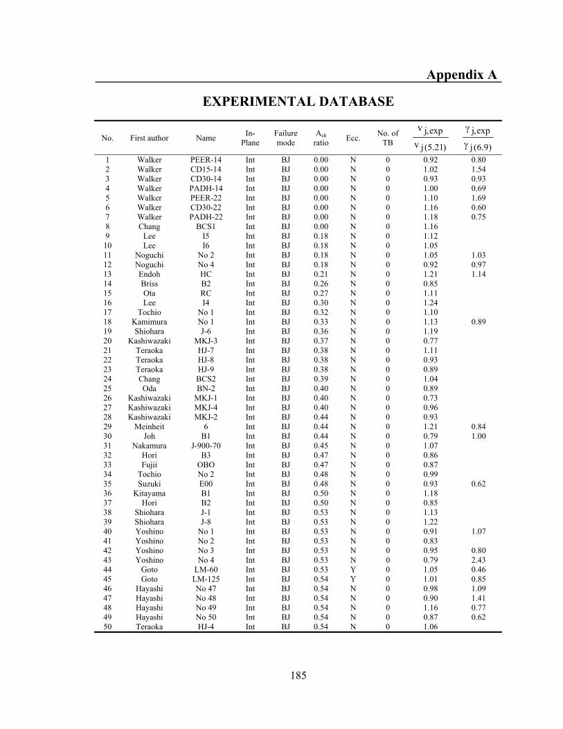
185

Appendix A

EXPERIMENTAL DATABASE

No. First author Name In-Plane

Failure mode

Ash ratio Ecc. No. of

TB )21.5(j

exp,jv

v

)9.6(j

exp,jγ

γ

1 Walker PEER-14 Int BJ 0.00 N 0 0.92 0.80 2 Walker CD15-14 Int BJ 0.00 N 0 1.02 1.54 3 Walker CD30-14 Int BJ 0.00 N 0 0.93 0.93 4 Walker PADH-14 Int BJ 0.00 N 0 1.00 0.69 5 Walker PEER-22 Int BJ 0.00 N 0 1.10 1.69 6 Walker CD30-22 Int BJ 0.00 N 0 1.16 0.60 7 Walker PADH-22 Int BJ 0.00 N 0 1.18 0.75 8 Chang BCS1 Int BJ 0.00 N 0 1.16 9 Lee I5 Int BJ 0.18 N 0 1.12

10 Lee I6 Int BJ 0.18 N 0 1.05 11 Noguchi No 2 Int BJ 0.18 N 0 1.05 1.03 12 Noguchi No 4 Int BJ 0.18 N 0 0.92 0.97 13 Endoh HC Int BJ 0.21 N 0 1.21 1.14 14 Briss B2 Int BJ 0.26 N 0 0.85 15 Ota RC Int BJ 0.27 N 0 1.11 16 Lee I4 Int BJ 0.30 N 0 1.24 17 Tochio No 1 Int BJ 0.32 N 0 1.10 18 Kamimura No 1 Int BJ 0.33 N 0 1.13 0.89 19 Shiohara J-6 Int BJ 0.36 N 0 1.19 20 Kashiwazaki MKJ-3 Int BJ 0.37 N 0 0.77 21 Teraoka HJ-7 Int BJ 0.38 N 0 1.11 22 Teraoka HJ-8 Int BJ 0.38 N 0 0.93 23 Teraoka HJ-9 Int BJ 0.38 N 0 0.89 24 Chang BCS2 Int BJ 0.39 N 0 1.04 25 Oda BN-2 Int BJ 0.40 N 0 0.89 26 Kashiwazaki MKJ-1 Int BJ 0.40 N 0 0.73 27 Kashiwazaki MKJ-4 Int BJ 0.40 N 0 0.96 28 Kashiwazaki MKJ-2 Int BJ 0.44 N 0 0.93 29 Meinheit 6 Int BJ 0.44 N 0 1.21 0.84 30 Joh B1 Int BJ 0.44 N 0 0.79 1.00 31 Nakamura J-900-70 Int BJ 0.45 N 0 1.07 32 Hori B3 Int BJ 0.47 N 0 0.86 33 Fujii OBO Int BJ 0.47 N 0 0.87 34 Tochio No 2 Int BJ 0.48 N 0 0.99 35 Suzuki E00 Int BJ 0.48 N 0 0.93 0.62 36 Kitayama B1 Int BJ 0.50 N 0 1.18 37 Hori B2 Int BJ 0.50 N 0 0.85 38 Shiohara J-1 Int BJ 0.53 N 0 1.13 39 Shiohara J-8 Int BJ 0.53 N 0 1.22 40 Yoshino No 1 Int BJ 0.53 N 0 0.91 1.07 41 Yoshino No 2 Int BJ 0.53 N 0 0.83 42 Yoshino No 3 Int BJ 0.53 N 0 0.95 0.80 43 Yoshino No 4 Int BJ 0.53 N 0 0.79 2.43 44 Goto LM-60 Int BJ 0.53 Y 0 1.05 0.46 45 Goto LM-125 Int BJ 0.54 Y 0 1.01 0.85 46 Hayashi No 47 Int BJ 0.54 N 0 0.98 1.09 47 Hayashi No 48 Int BJ 0.54 N 0 0.90 1.41 48 Hayashi No 49 Int BJ 0.54 N 0 1.16 0.77 49 Hayashi No 50 Int BJ 0.54 N 0 0.87 0.62 50 Teraoka HJ-4 Int BJ 0.54 N 0 1.06

186

No. First author Name In-

Plane Failure mode

Ash ratio Ecc. No. of

TB )21.5(j

exp,jv

v

)9.6(j

exp,jγ

γ

51 Teraoka HJ-5 Int BJ 0.54 N 0 0.92 52 Teraoka HJ-6 Int BJ 0.54 N 0 0.89 53 Kitayama I3 Int BJ 0.54 N 0 1.30 1.34 54 Nakamura J-600-70C Int BJ 0.55 N 0 1.13 55 Hori B1 Int BJ 0.57 N 0 0.87 56 Kamumura NN2 Int BJ 0.59 Y 0 0.84 57 Shiohara J-4 Int BJ 0.59 N 0 1.28 58 Shiohara J-5 Int BJ 0.59 N 0 1.19 59 Teraoka HNO 5 Int BJ 0.60 N 0 1.40 0.66 60 Teraoka HNO 6 Int BJ 0.60 N 0 1.18 0.55 61 Teraoka HNO 7 Int BJ 0.60 N 0 1.28 0.48 62 Goto HM-60 Int BJ 0.60 Y 0 1.19 1.34 63 Goto PL Int BJ 0.63 N 0 0.91 1.06 64 Nakamura J-600-50 Int BJ 0.64 N 0 0.98 65 Joh PL-13 Int BJ 0.64 N 0 0.93 66 Kitayama A4 Int BJ 0.65 N 0 1.22 67 Nakamura J-600-70A Int BJ 0.65 N 0 1.07 68 Kushuhara JE-0 Int BJ 0.65 N 0 1.09 0.77 69 Kusuhara JE-55 Int BJ 0.65 Y 0 1.07 0.48 70 Nakamura J-600-70B Int BJ 0.66 N 0 1.15 71 Teng S1 Int BJ 0.66 N 0 1.04 0.75 72 Kawai I8C Int BJ 0.69 N 0 0.90 73 Tsubosaki J-13-NS Int BJ 0.70 N 1 0.97 74 Goto HM-125 Int BJ 0.70 Y 0 1.19 0.75 75 Suzuki E00s Int BJ 0.70 N 1 1.23 76 Kitayama B2 Int BJ 0.70 N 0 1.14 1.32 77 Inoue SP2 Int BJ 0.71 N 0 0.82 78 Kamimura No 2 Int BJ 0.71 N 0 1.06 79 Ishida HS-HS Int BJ 0.71 N 0 0.72 80 Teraoka HNO1 Int BJ 0.72 N 0 1.13 0.66 81 Teraoka HNO2 Int BJ 0.72 N 0 1.43 0.80 82 Teraoka HNO3 Int BJ 0.72 N 0 1.34 0.74 83 Teraoka HNO4 Int BJ 0.72 N 0 1.19 0.76 84 Kamimura A-1 Int BJ 0.73 N 0 1.13 0.62 85 Saka INS Int BJ 0.74 N 0 1.00 86 Leon BCJ2 Int BJ 0.77 N 0 0.98 1.47 87 Tochio No 3 Int BJ 0.79 N 0 1.48 88 Shin S2 Int BJ 0.80 Y 1 0.88 0.90 89 Goto HH-125 Int BJ 0.80 Y 0 1.12 0.76 90 Oda BN-4 Int BJ 0.80 N 0 0.88 91 Kitayama J1 Int BJ 0.81 N 0 1.16 92 Hayashi No 35 Int BJ 0.85 Y 0 0.85 0.96 93 Hayashi No 38 Int BJ 0.85 Y 0 0.94 0.86 94 hayashi No 34 Int BJ 0.85 N 0 0.72 95 hayashi No 36 Int BJ 0.85 N 0 0.91 96 Joh PH-13 Int BJ 0.85 N 0 1.04 97 Leon BCJ3 Int BJ 0.85 N 0 0.87 1.06 98 Goto B17-13,X Int BJ 0.86 N 2 0.97 99 Fujii GBSU,E Int BJ 0.87 N 1 0.86 0.95

100 Joh PH-10 Int BJ 0.87 N 0 1.12

187

No. First author Name In-

Plane Failure mode

Ash ratio Ecc. No. of

TB )21.5(j

exp,jv

v

)9.6(j

exp,jγ

γ

101 Durrani X1 Int BJ 0.90 N 0 1.03 102 Goto HU-125 Int BJ 0.90 Y 0 1.10 0.74 103 Kaku J11B Int BJ 0.93 N 0 1.27 104 Joh PH-16 Int BJ 0.94 N 0 0.96 105 Noguchi OKJ-1 Int BJ 0.96 N 0 0.96 1.22 106 Kaku J11A Int BJ 0.96 N 0 1.02 0.89 107 Kaku J12C Int BJ 0.96 N 0 1.31 0.81 108 Shin S1 Int BJ 0.96 Y 1 0.88 1.10 109 Goto B17-19,X Int BJ 0.96 N 2 1.00 110 Shiohara 7 Int BJ 0.97 N 0 1.06 111 Kaku J12A Int BJ 0.98 N 0 1.17 0.62 112 Kaku J12B Int BJ 0.98 N 0 1.17 0.76 113 Meinheit 8 Int BJ 0.98 N 2 0.92 1.25 114 Goto B17-13L,X Int BJ 0.99 N 2 1.07 115 Tochio J1 Int BJ 1.01 N 0 1.36 116 Kaku J31A Int BJ 1.01 N 0 0.93 117 Kaku J31B Int BJ 1.01 N 0 0.98 118 Kamimura No 3 Int BJ 1.04 N 0 0.96 1.45 119 Raffaelle 3 Int BJ 1.04 Y 0 0.75 0.98 120 Kurose J3,N Int BJ 1.05 N 1 0.88 1.11 121 Briss B1 Int BJ 1.06 N 0 0.69 122 Teng S3 Int BJ 1.10 Y 0 1.15 0.96 123 Teng S2 Int BJ 1.13 Y 0 1.03 0.75 124 Shiohara 6 Int BJ 1.14 N 0 1.15 125 Tateishi CSP Int BJ 1.18 N 0 0.93 126 Kitayama B3 Int BJ 1.19 N 0 0.94 127 Teng S5 Int BJ 1.22 Y 0 1.26 0.59 128 Shin S4 Int BJ 1.23 N 1 1.09 1.98 129 Teng S6 Int BJ 1.25 Y 0 1.34 0.85 130 Nakamura J-600-70T Int BJ 1.27 N 2 0.93 131 Kusuhara JE-55S Int BJ 1.30 Y 0 1.01 1.03 132 Shiohara 8 Int BJ 1.31 N 0 1.02 133 Kaku J32A Int BJ 1.33 N 0 1.13 0.70 134 Kaku J32B Int BJ 1.35 N 0 1.14 135 Durrani X2 Int BJ 1.37 N 0 0.93 136 Raffaelle 1 Int BJ 1.37 Y 0 0.90 0.98 137 Goto PH Int BJ 1.40 N 0 0.83 1.27 138 Tsubosaki J-12-NS Int BJ 1.40 N 2 1.23 0.86 139 Noguchi OKJ-4 Int BJ 1.44 N 0 0.95 1.35 140 Raffaelle 2 Int BJ 1.46 Y 0 0.75 0.80 141 Asou No 1 Int BJ 1.46 N 0 0.86 142 Sugano J8H-0 Int BJ 1.54 N 1 0.94 143 Tateishi AIJ Int BJ 1.55 N 0 0.83 144 Tateishi JCR Int BJ 1.57 N 0 0.98 145 Tateishi HBS Int BJ 1.57 N 0 1.10 146 Sugano J8-0 Int BJ 1.59 N 1 0.98 147 Kurose J1 Int BJ 1.74 N 1 1.05 2.91 148 Watanabe WJ-1 Int BJ 1.86 N 0 1.11 0.56 149 Watanabe WJ-3 Int BJ 1.86 N 0 1.26 0.57 150 Guimaraes J6,E Int BJ 2.02 N 2 0.95 0.36

188

No. First author Name In-

Plane Failure mode

Ash ratio Ecc. No. of

TB )21.5(j

exp,jv

v

)9.6(j

exp,jγ

γ

151 Raffaelle 4 Int BJ 2.03 Y 0 0.88 1.36 152 Sugano J6-0 Int BJ 2.04 N 1 1.02 153 Guimaraes J4,E Int BJ 2.07 N 2 1.11 0.76 154 Meinheit 12 Int BJ 2.22 N 0 1.11 0.56 155 Guimaraes J5,E Int BJ 2.88 N 2 1.04 0.43 156 Kurose J2,E Int BJ 2.97 N 2 1.09 0.90 157 Tateishi HRP Int BJ 3.54 N 0 0.82 158 Meinheit 4 Int J 0.30 N 0 1.05 0.70 159 Suzuki E135 Int J 0.30 Y 0 0.88 1.25 160 Meinheit 2 Int J 0.39 N 0 1.18 0.74 161 Fujii A1 Int J 0.40 N 0 0.85 1.46 162 Fujii A2 Int J 0.40 N 0 1.07 2.67 163 Fujii A3 Int J 0.40 N 0 0.87 1.58 164 Meinheit 11 Int J 0.42 N 2 1.07 1.85 165 Meinheit 7 Int J 0.44 N 0 1.15 0.85 166 Meinheit 5 Int J 0.45 N 0 1.19 0.84 167 Goto UM-125 Int J 0.48 Y 0 1.00 0.90 168 Goto UM-60 Int J 0.49 Y 0 1.04 1.73 169 Suzuki E085 Int J 0.50 Y 0 1.07 1.52 170 Shiohara J-11 Int J 0.51 N 0 1.08 171 Goto UM-0 Int J 0.51 N 0 1.02 0.60 172 Meinheit 9 Int J 0.52 N 2 1.07 1.05 173 Meinheit 10 Int J 0.55 N 2 1.03 0.85 174 Hosono TD-1-F Int J 0.58 N 2 0.99 175 Nakamura J-600-70 Int J 0.61 N 0 0.94 176 Meinheit 3 Int J 0.61 N 0 1.04 0.46 177 Meinheit 1 Int J 0.62 N 0 0.94 0.44 178 Endoh A1 Int J 0.65 N 0 1.08 1.47 179 Goto UU-125 Int J 0.68 Y 0 0.95 1.42 180 Shiohara 11 Int J 0.70 N 0 1.11 181 Shiohara 9 Int J 0.70 N 0 1.06 182 Shiohara J2 Int J 0.72 N 0 0.89 183 Shiohara J3 Int J 0.72 N 0 0.92 184 Kitayama A1 Int J 0.73 N 0 1.16 185 Shiohara S3 Int J 0.91 N 0 1.03 0.34 186 Noguchi OKJ-3 Int J 0.94 N 0 0.96 1.09 187 Morita No 4 Int J 0.94 N 0 1.21 188 Noguchi OKJ-5 Int J 0.96 N 0 0.95 0.93 189 Morita No 1 Int J 0.96 N 0 1.15 0.43 190 Meinheit 14 Int J 0.98 N 0 1.27 1.09 191 Fujii A4 Int J 1.08 N 0 0.80 1.23 192 Shiohara J10 Int J 1.10 N 0 1.04 0.63 193 Meinheit 13 Int J 1.18 N 0 1.01 0.56 194 Shiohara 4 Int J 1.23 N 0 1.14 195 Noguchi OKJ-6 Int J 1.25 N 0 0.93 0.87 196 Shiohara 3 Int J 1.31 N 0 1.06 197 Shiohara 1 Int J 1.34 N 0 1.07 198 Morita No 5 Int J 1.47 N 0 1.26 199 Shiohara 12 Int J 1.58 N 0 1.02 200 Shiohara 10 Int J 1.67 N 0 0.97

189

No. First author Name In-

Plane Failure mode

Ash ratio Ecc. No. of

TB )21.5(j

exp,jv

v

)9.6(j

exp,jγ

γ

201 Shiohara 5 Int J 1.67 N 0 1.10 202 Owada J0-1 Int J 1.70 N 0 0.80 203 Owada J0-2 Int J 1.70 N 0 0.88 204 Owada JE-1 Int J 1.70 N 1 0.88 205 Shiohara 2 Int J 1.82 N 0 1.04 206 Watanabe WJ-6 Int J 1.86 N 0 1.33 0.76 207 Besso J3 Int J 2.06 N 2 0.90 208 Besso J1 Int J 2.19 N 0 1.01 209 Besso J2 Int J 2.19 N 1 1.01 210 Tateishi KSC Int J 3.38 N 0 1.02 211 Owada JI-1 Int J 3.39 N 2 0.90 212 Sugano J4-0 Int J 4.07 N 1 0.94 213 Uzumeri 2 Ext BJ 0.00 N 0 0.98 214 Ohnish No 1 Ext BJ 0.00 N 0 0.72 215 Ohnish No 4 Ext BJ 0.00 N 0 1.17 216 Shin HJC0-RO Ext BJ 0.00 N 0 0.85 217 Mituwa No 17 Ext BJ 0.00 N 0 0.93 218 Hwang 0T0 Ext BJ 0.00 N 0 0.83 219 Hwang 1B8 Ext BJ 0.00 N 0 1.08 220 Shin HJC1-RO Ext BJ 0.09 N 0 1.10 221 Kaku No 11 Ext BJ 0.10 N 0 0.97 1.16 222 Kaku No 6 Ext BJ 0.10 N 0 0.89 0.76 223 Kaku No 14 Ext BJ 0.10 N 0 0.96 1.16 224 Kaku No 15 Ext BJ 0.11 N 0 0.99 1.40 225 Kaku No 5 Ext BJ 0.11 N 0 0.96 1.00 226 Kaku No 12 Ext BJ 0.12 N 0 0.92 0.95 227 Shin HJC2-RO Ext BJ 0.14 N 0 1.12 228 Shin HJC3-RO Ext BJ 0.18 N 0 0.94 229 Ohnish No 2 Ext BJ 0.19 N 0 0.72 230 Hwang 1T44 Ext BJ 0.22 N 0 0.81 231 Lee 6 Ext BJ 0.23 N 0 0.84 232 Hwang 2T4 Ext BJ 0.23 N 0 0.84 233 Mituwa No 19 Ext BJ 0.24 N 0 0.87 234 Joh NRC-J12 Ext BJ 0.26 N 0 0.91 0.80 235 Hwang 3T3 Ext BJ 0.28 N 0 0.85 236 Kawai O8V Ext BJ 0.34 N 0 0.95 237 Ohnish No 3 Ext BJ 0.34 N 0 0.61 238 Kaku No 13 Ext BJ 0.35 N 0 0.69 0.78 239 Sekine No 8 Ext BJ 0.36 N 0 0.71 240 Ohnish No 5 Ext BJ 0.38 N 0 0.91 241 Kaku No 3 Ext BJ 0.39 N 0 0.74 1.11 242 Kaku No 9 Ext BJ 0.40 N 0 0.81 2.79 243 Hanson S4 Ext BJ 0.41 N 0 1.16 244 Sekine No 6 Ext BJ 0.42 N 0 0.72 245 Ehsani LL14 Ext BJ 0.42 N 0 0.98 246 Sekine No 7 Ext BJ 0.42 N 0 0.74 247 Kaneda U41L Ext BJ 0.53 N 0 0.90 248 Fujii B2 Ext BJ 0.55 N 0 0.96 0.71 249 Oh 400-0.6N Ext BJ 0.60 N 0 1.05 250 Oh 400-0.6N' Ext BJ 0.60 N 0 1.03

190

No. First author Name In-

Plane Failure mode

Ash ratio Ecc. No. of

TB )21.5(j

exp,jv

v

)9.6(j

exp,jγ

γ

251 Ehsani LH14 Ext BJ 0.63 N 0 0.96 252 Ehsani HH14 Ext BJ 0.63 N 0 0.79 253 Tsubosaki J-13-E Ext BJ 0.70 N 2 0.83 254 Uzumeri 3 Ext BJ 0.70 N 1 1.05 255 Hanson 1-A Ext BJ 0.71 N 0 1.02 256 Ehsani LL8 Ext BJ 0.72 N 0 0.91 2.04 257 Ehsani LH11 Ext BJ 0.79 N 0 1.00 258 Ehsani HH11 Ext BJ 0.79 N 0 0.89 259 Mituwa No 21 Ext BJ 0.86 N 0 0.88 260 Fujii GBSU,N Ext BJ 0.87 N 2 1.03 1.45 261 Ehsani 3B Ext BJ 0.91 N 0 1.17 1.15 262 Ehsani 4B Ext BJ 0.91 N 0 1.19 1.78 263 Kaneda U42L Ext BJ 0.94 N 0 0.76 264 Uzumeri 7 Ext BJ 0.96 N 0 0.93 265 Joh NRC-J13 Ext BJ 0.97 N 0 1.03 0.56 266 Mituwa No 18 Ext BJ 0.99 N 0 0.92 267 Tsonos S6' Ext BJ 0.99 N 0 1.09 268 Uzumeri 4 Ext BJ 0.99 N 1 1.09 269 Kurose J3,E Ext BJ 1.05 N 2 1.27 1.15 270 Nishiyama RC2 Ext BJ 1.06 N 0 271 Ehsani LH8 Ext BJ 1.08 N 0 0.83 1.83 272 Ehsani HH8 Ext BJ 1.08 N 0 0.97 1.91 273 Hamada J-10 Ext BJ 1.09 N 0 0.88 274 Ehsani 4 Ext BJ 1.11 N 0 0.99 275 Tsonos MS4 Ext BJ 1.11 N 0 0.90 276 Ehsani 3 Ext BJ 1.15 N 0 0.98 277 Ehsani 3S Ext BJ 1.15 N 2 0.81 278 Paulay Unit 2 Ext BJ 1.19 N 0 0.90 279 Chutsrat Specimen1 Ext BJ 1.32 N 0 0.86 280 Uzumeri 6 Ext BJ 1.37 N 0 0.86 281 Mituwa No 22 Ext BJ 1.47 N 0 0.80 282 Tsonos S3 Ext BJ 1.51 N 0 0.88 283 Mituwa No 20 Ext BJ 1.61 N 0 0.72 284 Megget Unit A Ext BJ 1.76 N 0 0.97 1.48 285 Uzumeri 8 Ext BJ 1.92 N 0 0.95 286 Kaneda U40L Ext J 0.00 N 0 0.81 287 Oh 200-0 Ext J 0.00 N 0 1.07 288 Oh 400-0 Ext J 0.00 N 0 1.11 289 Joh LO-N96 Ext J 0.24 N 0 0.97 0.71 290 Joh LO-NO Ext J 0.27 N 0 0.88 0.68 291 Oh 400-0.3N Ext J 0.39 N 0 1.15 292 Joh NRC-J8 Ext J 0.40 N 0 0.96 0.96 293 Ehsani HL14 Ext J 0.42 N 0 0.85 294 Lee HJ2+0.0 Ext J 0.43 N 0 0.81 295 Kaku No 22 Ext J 0.45 N 0 0.72 1.96 296 Ehsani LL11 Ext J 0.54 N 0 0.77 297 Ehsani HL11 Ext J 0.54 N 0 0.82 298 Fujii B1 Ext J 0.55 N 0 0.83 1.59 299 Fujii B3 Ext J 0.55 N 0 0.93 1.33 300 Oh 200-0.3N Ext J 0.61 N 0 1.15

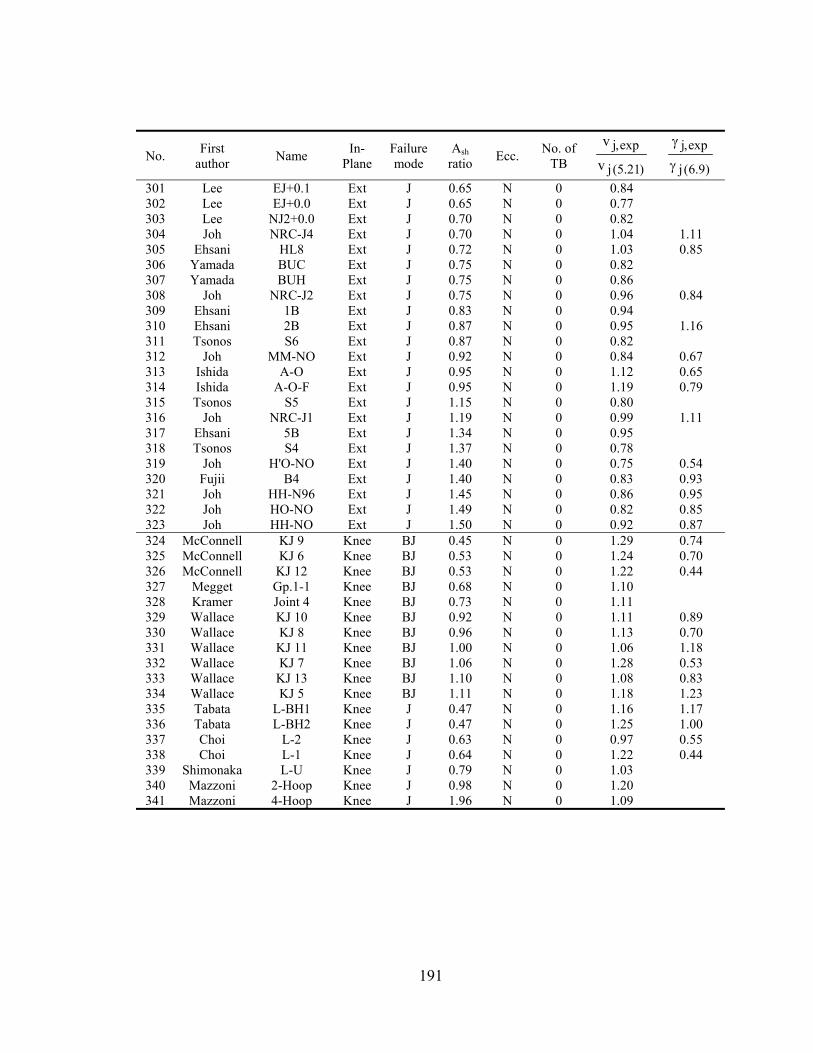
191

No. First author Name In-

Plane Failure mode

Ash ratio Ecc. No. of

TB )21.5(j

exp,jv

v

)9.6(j

exp,jγ

γ

301 Lee EJ+0.1 Ext J 0.65 N 0 0.84 302 Lee EJ+0.0 Ext J 0.65 N 0 0.77 303 Lee NJ2+0.0 Ext J 0.70 N 0 0.82 304 Joh NRC-J4 Ext J 0.70 N 0 1.04 1.11 305 Ehsani HL8 Ext J 0.72 N 0 1.03 0.85 306 Yamada BUC Ext J 0.75 N 0 0.82 307 Yamada BUH Ext J 0.75 N 0 0.86 308 Joh NRC-J2 Ext J 0.75 N 0 0.96 0.84 309 Ehsani 1B Ext J 0.83 N 0 0.94 310 Ehsani 2B Ext J 0.87 N 0 0.95 1.16 311 Tsonos S6 Ext J 0.87 N 0 0.82 312 Joh MM-NO Ext J 0.92 N 0 0.84 0.67 313 Ishida A-O Ext J 0.95 N 0 1.12 0.65 314 Ishida A-O-F Ext J 0.95 N 0 1.19 0.79 315 Tsonos S5 Ext J 1.15 N 0 0.80 316 Joh NRC-J1 Ext J 1.19 N 0 0.99 1.11 317 Ehsani 5B Ext J 1.34 N 0 0.95 318 Tsonos S4 Ext J 1.37 N 0 0.78 319 Joh H'O-NO Ext J 1.40 N 0 0.75 0.54 320 Fujii B4 Ext J 1.40 N 0 0.83 0.93 321 Joh HH-N96 Ext J 1.45 N 0 0.86 0.95 322 Joh HO-NO Ext J 1.49 N 0 0.82 0.85 323 Joh HH-NO Ext J 1.50 N 0 0.92 0.87 324 McConnell KJ 9 Knee BJ 0.45 N 0 1.29 0.74 325 McConnell KJ 6 Knee BJ 0.53 N 0 1.24 0.70 326 McConnell KJ 12 Knee BJ 0.53 N 0 1.22 0.44 327 Megget Gp.1-1 Knee BJ 0.68 N 0 1.10 328 Kramer Joint 4 Knee BJ 0.73 N 0 1.11 329 Wallace KJ 10 Knee BJ 0.92 N 0 1.11 0.89 330 Wallace KJ 8 Knee BJ 0.96 N 0 1.13 0.70 331 Wallace KJ 11 Knee BJ 1.00 N 0 1.06 1.18 332 Wallace KJ 7 Knee BJ 1.06 N 0 1.28 0.53 333 Wallace KJ 13 Knee BJ 1.10 N 0 1.08 0.83 334 Wallace KJ 5 Knee BJ 1.11 N 0 1.18 1.23 335 Tabata L-BH1 Knee J 0.47 N 0 1.16 1.17 336 Tabata L-BH2 Knee J 0.47 N 0 1.25 1.00 337 Choi L-2 Knee J 0.63 N 0 0.97 0.55 338 Choi L-1 Knee J 0.64 N 0 1.22 0.44 339 Shimonaka L-U Knee J 0.79 N 0 1.03 340 Mazzoni 2-Hoop Knee J 0.98 N 0 1.20 341 Mazzoni 4-Hoop Knee J 1.96 N 0 1.09

192

Appendix B

JOINT SHEAR BEHAVIOR PLOT RESULTS

Subassembly conditions: Equal to or above 0.70 in Ash ratio; No out-of-plane; and No joint eccentricity

0

5

10

15

20

25

30

0.00 0.01 0.02 0.03 0.04 0.05

Joint shear strain (Radian)

Join

t she

ar s

tres

s (M

Pa)

ExperimentSimple and unified modelFEMA 356TeraokaParra-Montesinos and WightModified Parra-Montesinos and Wight modelMCFT

Meinheit: 12 (Interior)

0

5

10

15

20

25

30

0.00 0.01 0.02 0.03 0.04 0.05

Joint shear strain (Rad)Jo

int s

hear

str

ess

(MPa

)

Experimentsimple and unified modellFEMA 356TeraokaParra-Montesinos and WightModified Parra-Montesinos and Wight modelMCFT

Watanabe: WJ-1 (Interior)

0

5

10

15

20

25

30

0.00 0.01 0.02 0.03 0.04 0.05

Joint shear strain (Rad)

Join

t she

ar s

tres

s (M

Pa)

ExperimentSimple and unified modellFEMA 356TeraokaParra-Montesinos and WightModified Parra-Montesinos and Wight modelMCFT

Watanabe: WJ-3 (Interior)

0

5

10

15

20

25

30

0.00 0.01 0.02 0.03 0.04 0.05

Joint shear strain (Rad)

Join

t she

ar s

tres

s (M

Pa)

ExperimentSimple and unified modelFEMA 356TeraokaParra-Montesinos and WightModified Parra-Montesinos and Wight modelMCFT

Leon: BCJ 2 (Interior)

0

5

10

15

20

25

30

0.00 0.01 0.02 0.03 0.04 0.05

Joint shear strain (Rad)

Join

t she

ar s

tres

s (M

Pa)

ExperimentSimple and unified modelFEMA 356TeraokaParra-Montesinos and WightModified Parra-Montesinos and Wight modelMCFT

Leon: BCJ 3 (Interior)

0

5

10

15

20

25

30

0.00 0.01 0.02 0.03 0.04 0.05

Joint shear strain (Rad)

Join

t she

ar s

tres

s (M

Pa)

ExperimentSimple and unified modelFEMA 356Teraoka and FujiiParra-Montesinos and WightModified Parra-Montesinos and Wight modelMCFT

Noguchi: OKJ 1 (Interior)

193

0

5

10

15

20

25

30

0.00 0.01 0.02 0.03 0.04 0.05

Joint shear strain (Rad)

Join

t she

ar s

tres

s (M

Pa)

ExperimentSimple and unified modelFEMA 356TeraokaParra-Montesinos and WightModified Parra-Montesinos and Wight modelMCFT

Noguchi: OKJ 4 (Interior)

0

5

10

15

20

25

30

0.00 0.01 0.02 0.03 0.04 0.05

Joint shear strain (Rad)

Join

t she

ar s

tres

s (M

Pa)

ExperimentSimple and unified modellFEMA 356TeraokaParra-Montesinos and WightModified Parra-Montesinos and Wight modelMCFT

Goto: PH (Interior)

0

5

10

15

20

25

30

0.00 0.01 0.02 0.03 0.04 0.05

Joint shear strain (Rad)

Join

t she

ar s

tres

s (M

Pa)

ExperimentSimple and unified modelFEMA 356TeraokaParra-Montesinos and WightModified Parra-Montesinos and Wight modelMCFT

Kaku: J11A (Interior)

0

5

10

15

20

25

30

0.00 0.01 0.02 0.03 0.04 0.05

Joint shear strain (Rad)

Join

t she

ar s

tres

s (M

Pa)

ExperimentSimple and unified modellFEMA 356TeraokaParra-Montesinos and WightModified Parra-Montesinos and Wight modelMCFT

Kaku: J12A (Interior)

0

5

10

15

20

25

30

0.00 0.01 0.02 0.03 0.04 0.05

Joint shear strain (Rad)

Join

t she

ar s

tres

s (M

Pa)

ExperimentSimple and unified modelFEMA 356TeraokaParra-Montesinos and WightModified Parra-Montesinos and Wight modelMCFT

Kaku: J12B (interior)

0

5

10

15

20

25

30

0.00 0.01 0.02 0.03 0.04 0.05

Joint shear strain (Rad)

Join

t she

ar s

tres

s (M

Pa)

ExperimentSimple and unified modelFEMA 356TeraokaParra-Montesinos and WightModified Parra-Montesinos and Wight modelMCFT

Kaku: J12C (Interior)

0

5

10

15

20

25

30

0.00 0.01 0.02 0.03 0.04 0.05

Joint shear strain (Rad)

Join

t she

ar s

tres

s (M

Pa)

Experiment

Simple and unified model

FEMA 356

Teraoka

Parra-Montesinos and Wight

Modified Parra-Montesinos and Wight model

MCFT

Kaku: J32A (Interior)

0

5

10

15

20

25

30

0.00 0.01 0.02 0.03 0.04 0.05

Joint shear strain (Rad)

Join

t she

ar s

tres

s (M

Pa)

ExperimentSimple and unified modelFEMA 356TeraokaParra-Montesinos and WightModified Parra-Montesinos and Wight modelMCFT

Kamimura: No 3 (Interior)

194

0

5

10

15

20

25

30

0.00 0.01 0.02 0.03 0.04 0.05

Joint shear strain (Rad)

Join

t she

ar s

tres

s (M

Pa)

ExperimentSimple and unified modelFEMA 356TeraokaParra-Montesinos and WightModified Parra-Montesinos and Wight modelMCFT

Kitayama: B2 (Interior)

0

5

10

15

20

25

30

0.00 0.01 0.02 0.03 0.04 0.05

Joint shear strain (Rad)

Join

t she

ar s

tres

s (M

Pa)

ExperimentSimple and unified modelFEMA 356TeraokaParra-Montesinos and WightModified Parra-Montesinos and Wight modelMCFT

Kamimura: A1 (Interior)

0

5

10

15

20

25

30

0.00 0.01 0.02 0.03 0.04 0.05

Joint shear strain (Rad)

Join

t she

ar s

tres

s (M

Pa)

ExperimentSimple and unified modelFEMA 356TeraokaParra-Montesinos and WightModified Parra-Montesinos and Wight modelMCFT

Meinheit: 13 (Interior)

0

5

10

15

20

25

30

0.00 0.01 0.02 0.03 0.04 0.05

Joint shear strain (Rad)

Join

t she

ar s

tres

s (M

Pa)

ExperimentSimple and unified modelFEMA 356TeraokaParra-Montesinos and WightModified Parra-Montesinos and Wight modelMCFT

Meinheit: 14 (Interior)

0

5

10

15

20

25

30

0.00 0.01 0.02 0.03 0.04 0.05

Joint shear strain (Rad)

Join

t she

ar s

tres

s (M

Pa)

ExperimentSimple and unified modelFEMA 356TeraokaParra-Montesinos and WightModified Parra-Montesinos and WigthMCFT

Watanabe: WJ-6 (Interior)

0

5

10

15

20

25

30

0.00 0.01 0.02 0.03 0.04 0.05

Joint shear strain (Rad)

Join

t she

ar s

tres

s (M

Pa)

ExperimentSimple and unified modelFEMA 356TeraokaParra-Montesinos and WightModified Parra-Montesinos and WightMCFT

Fujii: A4 (Interior)

0

5

10

15

20

25

30

0.00 0.01 0.02 0.03 0.04 0.05

Joint shear strain (Rad)

Join

t she

ar s

tres

s (M

Pa)

ExperimentSimple and unified modelFEMA 356TeraokaParra-Montesinos and WightModified Parra-Montesinos and WightMCFT

Noguchi: OKJ3 (Interior)

0

5

10

15

20

25

30

0.00 0.01 0.02 0.03 0.04 0.05

Joint shear strain (Rad)

Join

t she

ar s

tres

s (M

Pa)

ExperimentSimple and unified modelFEMA 356TeraokaParra-Montesinos and WightModified Parra-Montesinos and WightMCFT

Noguchi: OKJ5 (Interior)

195

0

5

10

15

20

25

30

0.00 0.01 0.02 0.03 0.04 0.05

Joint shear strain (Rad)

Join

t she

ar s

tres

s (M

Pa)

ExperimentSimple and unified modelFEMA 356TeraokaParra-Montesinos and WightModified Parra-Montesinos and WightMCFT

Noguchi: OKJ6 (Interior)

0

5

10

15

20

25

30

0.00 0.01 0.02 0.03 0.04 0.05

Joint shear strain (Rad)

Join

t she

ar s

tres

s (M

Pa)

ExperimentSimple and unified modelFEMA 356TeraokaParra-Montesinos and WightModified Parra-Montesinos and Wight modelMCFT

Morita: N1 (Interior)

0

5

10

15

20

25

30

0.00 0.01 0.02 0.03 0.04 0.05

Joint shear strain (Rad)

Join

t she

ar s

tres

s (M

Pa)

ExperimentSimple and unified modelFEMA 356TeraokaParra-Montesinos and WightModified Parra-Montesinos and Wight modelMCFT

Shiohara: J10 (Interior)

0

5

10

15

20

25

30

0.00 0.01 0.02 0.03 0.04 0.05

Joint shear strain (Rad)

Join

t she

ar s

tres

s (M

Pa)

ExperimentSimple and unified modelFEMA 356TeraokaParra-Montesinos and WightModified Parra-Montesinos and WightMCFT

Shiohara: S3 (Interior)

0

5

10

15

20

25

30

0.00 0.01 0.02 0.03 0.04 0.05

Joint shear strain (Rad)

Join

t she

ar s

tres

s (M

Pa)

ExperimentSimple and unified modelFEMA 356TeraokaParra-Montesinos and WigthModified Parra-Montesinos and WightMCFT

Megget: Unit A (Exterior)

0

5

10

15

20

25

30

0.00 0.01 0.02 0.03 0.04 0.05

Joint shear strain (Rad)

Join

t she

ar s

tres

s (M

Pa)

ExperimentSimple and unified modelFEMA 356TeraokaParra-Montesinos and WightModified Parra-Montesinos and WightMCFT

Ehsani: 3B (Exterior)

0

5

10

15

20

25

30

0.00 0.01 0.02 0.03 0.04 0.05

Joint shear strain (Rad)

Join

t she

ar s

tres

s (M

Pa)

ExperimentSimple and unified modelFEMA 356TeraokaParra-Montesinos and WightModified Parra-Montesinos and WightMCFT

Ehsani: 4B (Exterior)

0

5

10

15

20

25

30

0.00 0.01 0.02 0.03 0.04 0.05

Joint shear strain (Rad)

Join

t she

ar s

tres

s (M

Pa)

ExperimentSimple and unified modelFEMA 356TeraokaParra-Montesinos and WightModified Parra-Montesinos and WightMCFT

Ehsani: LH8 (Exterior)

196

0

5

10

15

20

25

30

0.00 0.01 0.02 0.03 0.04 0.05

Joint shear strain (Rad)

Join

t she

ar s

tres

s (M

Pa)

ExperimentSimple and unified modelFEMA 356TeraokaParra-Montesinos and WightModified Parra-Montesinos and WightMCFT

Ehsani: HH8 (Exterior)

0

5

10

15

20

25

30

0.00 0.01 0.02 0.03 0.04 0.05

Joint shear strain (Rad)

Join

t she

ar s

tres

s (M

Pa)

ExperimentSimple and unified modelFEMA 356TeraokaParra-Montesinos and WightModified Parra-Montesinos and WightMCFT

Joh: NRC-J13 (Exterior)

0

5

10

15

20

25

30

0.00 0.01 0.02 0.03 0.04 0.05

Joint shear strain (Rad)

Join

t she

ar s

tres

s (M

Pa)

ExperimentSimple and unified modelFEMA 356TeraokaParra-Montesinos and WightModified Parra-Montesinos and WightMCFT

Ehsani: LL8 (Exterior)

0

5

10

15

20

25

30

0.00 0.01 0.02 0.03 0.04 0.05

Joint shear strain (Rad)

Join

t she

ar s

tres

s (M

Pa)

ExperimentSimple and unified modelFEMA 356TeraokaParra-Montesinos and WightModified Parra-Montesinos and WightMCFT

Ehsani: 2B (Exterior)

0

5

10

15

20

25

30

0.00 0.01 0.02 0.03 0.04 0.05

Joint shear strain (Rad)

Join

t she

ar s

tres

s (M

Pa)

ExperimentSimple and unified modelFEMA 356TeraokaParra-Montesinos and WightModified Parra-Montesinos and WightMCFT

Joh: HO-NO (Exterior)

0

5

10

15

20

25

30

0.00 0.01 0.02 0.03 0.04 0.05

Joint shear strain (Rad)

Join

t she

ar s

tres

s (M

Pa)

ExperimentSimple and unified modelFEMA 356TeraokaParra-Montesinos and WightModified Parra-Montesinos and WightMCFT

Joh: MM-NO (Exterior)

0

5

10

15

20

25

30

0.00 0.01 0.02 0.03 0.04 0.05

Joint shear strain (Rad)

Join

t she

ar s

tres

s (M

Pa)

ExperimentSimple and unified modelFEMA 356TeraokaParra-Montesinos and WightModified Parra-Montesinos and WightMCFT

Joh: HH-NO (Exterior)

0

5

10

15

20

25

30

0.00 0.01 0.02 0.03 0.04 0.05

Joint shear strain (Rad)

Join

t she

ar s

tres

s (M

Pa)

ExperimentSimple and unified modelFEMA 356TeraokaParra-Montesinos and WightModified Parra-Montesinos and WightMCFT

Joh: H'O-NO (Exterior)

197

0

5

10

15

20

25

30

0.00 0.01 0.02 0.03 0.04 0.05

Joint shear strain (Rad)

Join

t she

ar s

tres

s (M

Pa)

ExperimentSimple and unified modelFEMA 356TeraokaParra-Montesinos and WightModified Parra-Montesinos and WightMCFT

Joh: HH-N96 (Exterior)

0

5

10

15

20

25

30

0.00 0.01 0.02 0.03 0.04 0.05

Joint shear strain (Rad)

Join

t she

ar s

tres

s (M

Pa)

ExperimentSimple and unified modelFEMA 356TeraokaParra-Montesinos and WightModified Parra-Montesinos and WightMCFT

Joh: NRC-J1 (Exterior)

0

5

10

15

20

25

30

0.00 0.01 0.02 0.03 0.04 0.05

Joint shear strain (Rad)

Join

t she

ar s

tres

s (M

Pa)

ExperimentSimple and unified modelFEMA 356TeraokaParra-Montesinos and WightModified Parra-Montesinos and WightMCFT

Ishida: AO (Exterior)

0

5

10

15

20

25

30

0.00 0.01 0.02 0.03 0.04 0.05

Joint shear strain (Rad)

Join

t she

ar s

tres

s (M

Pa)

Experimentsimple and unified modelFEMA 356TeraokaParra-Montesinos and WightModified Parra-Montesinos and WightMCFT

Ishida: AOF (Exterior)

0

5

10

15

20

25

30

0.00 0.01 0.02 0.03 0.04 0.05

Joint shear strain (Rad)

Join

t she

ar s

tres

s (M

Pa)

ExperimentSimple and unified modelFEMA 356TeraokaParra-Montesinos and WightModified Parra-Montesinos and WightMCFT

Ehsani: HL8 (Exterior)

0

5

10

15

20

25

30

0.00 0.01 0.02 0.03 0.04 0.05

Joint shear strain (Rad)

Join

t she

ar s

tres

s (M

Pa)

ExperimentSimple and unified modelFEMA 356TeraokaParra-Montesinos and WightModified Parra-Montesinos and WightMCFT

Joh: NRC-J2 (Exterior)

0

5

10

15

20

25

30

0.00 0.01 0.02 0.03 0.04 0.05

Joint shear strain (Rad)

Join

t she

ar s

tres

s (M

Pa)

ExperimentSimple and unified modelFEMA 356TeraokaParra-Montesinos and WightModified Parra-Montesinos and WightMCFT

Joh: NRJ-J4 (Exterior)

0

5

10

15

20

25

30

0 0.01 0.02 0.03 0.04 0.05

Joint shear strain (Rad)

Join

t she

ar s

tres

s (M

Pa)

ExperimentSimple and unified modelFEMA 356TeraokaModified Parra-Montesinos and WightMCFT

Wallace: KJ 5 (Knee)

198

0

5

10

15

20

25

30

0.00 0.01 0.02 0.03 0.04 0.05

Joint shear strain (Rad)

Join

t she

ar s

tres

s (M

Pa)

ExperimentSimple and unified modelFEMA 356TeraokaModified Parra-Montesinos and WightMCFT

Wallace: KJ 8 (Knee)

0

5

10

15

20

25

30

0.00 0.01 0.02 0.03 0.04 0.05

Joint shear strain (Rad)

Join

t she

ar s

tres

s (M

Pa)

ExperimentSimple and unified modelFEMA 356TeraokaModified Parra-Montesinos and WightMCFT

Wallace: KJ 10 (Knee)

0

5

10

15

20

25

30

0.00 0.01 0.02 0.03 0.04 0.05

Joint shear strain (Rad)

Join

t she

ar s

tres

s (M

Pa)

ExperimentSimple and unified modelFEMA 356TeraokaModified Parra-Montesinos and WightMCFT

Wallace: KJ 11 (Knee)

0

5

10

15

20

25

30

0.00 0.01 0.02 0.03 0.04 0.05

Joint shear strain (Rad)

Join

t she

ar s

tres

s (M

Pa)

ExperimentSimple and unified modelFEMA 356TeraokaModified Parra-Montesinos and WightMCFT

Wallace: KJ 13 (Knee)

Subassembly conditions: Equal to or above 0.70 in Ash ratio; With out-of-plane; and No joint eccentricity

0

5

10

15

20

25

30

0.00 0.01 0.02 0.03 0.04 0.05

Joint shear strain (Rad)

Join

t she

ar s

tres

s (M

Pa)

ExperimentSimple and unified modelFEMA 356TeraokaModified Parra-Montesinos and WightMCFT

Kurose: J1 (Interior)

0

5

10

15

20

25

30

0.00 0.01 0.02 0.03 0.04 0.05

Joint shear strain (Rad)

Join

t she

ar s

tres

s (M

Pa)

ExperimentSimple and unified modelFEMA 356TeraokaModified Parra-Montesinos and WightMCFT

Kurose: J3 N (Interior)

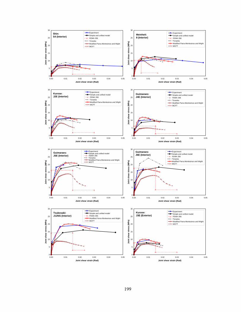
199

0

5

10

15

20

25

30

0.00 0.01 0.02 0.03 0.04 0.05

Joint shear strain (Rad)

Join

t she

ar s

trai

n (M

Pa)

ExperimentSimple and unified modelFEMA 356TeraokaModified Parra-Montesinos and WightMCFT

Shin: S4 (Interior)

0

5

10

15

20

25

30

0.00 0.01 0.02 0.03 0.04 0.05

Joint shear strain (Rad)

Join

t she

ar s

tres

s (M

Pa)

ExperimentSimple and unified modelFEMA 356TeraokaModified Parra-Montesinos and WightMCFT

Meinheit: 8 (Interior)

0

5

10

15

20

25

30

0.00 0.01 0.02 0.03 0.04 0.05

Joint shear strain (Rad)

Join

t she

ar s

tres

s (M

Pa)

ExperimentSimple and unified modelFEMA 356TeraokaModified Parra-Montesinos and WightMCFT

Kurose: J2E (Interior)

0

5

10

15

20

25

30

0.00 0.01 0.02 0.03 0.04 0.05

Joint shear strain (Rad)

Join

t she

ar s

tres

s (M

Pa)

ExperimentSimple and unified modelFEMA 356TeraokaModified Parra-Montesinos and WightMCFT

Guimaraes: J4E (Interior)

0

5

10

15

20

25

30

0.00 0.01 0.02 0.03 0.04 0.05

Joint shear strain (Rad)

Join

t she

ar s

tres

s (M

Pa)

ExperimentSimple and unified modelFEMA 356TeraokaModified Parra-Montesinos and WightMCFT

Guimaraes: J5E (Interior)

0

5

10

15

20

25

30

0.00 0.01 0.02 0.03 0.04 0.05

Joint shear strain (Rad)

Join

t she

ar s

tres

s (M

Pa)

ExperimentSimple and unified modelFEMA 356TeraokaModified Parra-Montesinos and WightMCFT

Guimaraes: J6E (Interior)

0

5

10

15

20

25

30

0.00 0.01 0.02 0.03 0.04 0.05

Joint shear strain (Rad)

Join

t she

ar s

tres

s (M

Pa)

ExperimentSimple and unified modelFEMA 356Modified Parra-Montesinos and WightMCFT

Tsubosaki: J12NS (Interior)

0

5

10

15

20

25

30

0.00 0.01 0.02 0.03 0.04 0.05

Joint shear strain (Rad)

Join

t she

ar s

tres

s (M

Pa)

ExperimentSimple and unified modelFEMA 356TeraokaModified Parra-Montesinos and WightMCFT

Kurose: J3E (Exterior)

200

Subassembly conditions: Equal to or above 0.70 in Ash ratio; No out-of-plane; and With joint eccentricity

0

5

10

15

20

25

30

0.00 0.01 0.02 0.03 0.04 0.05

Joint shear strain (Rad)

Join

t she

ar s

tres

s (M

Pa)

ExperimentSimple and unified modelFEMA 356TeraokaParra-Montesinos and WightModified Parra-Montesinos and WightMCFT

Hayashi: N35 (Interior)

0

5

10

15

20

25

30

0.00 0.01 0.02 0.03 0.04 0.05

Joint shear strain (Rad)

Join

t she

ar s

tres

s (M

Pa)

ExperimentSimple and unified modelFEMA 356TeraokaParra-Montesinos and WightModified Parra-Montesinos and WightMCFT

Goto: HM125 (Interior)

0

5

10

15

20

25

30

0.00 0.01 0.02 0.03 0.04 0.05

Joint shear strain (Rad)

Join

t she

ar s

tres

s (M

Pa)

ExperimentSimple and unified modelFEMA 356TeraokaParra-Montesinos and WightModified Parra-Montesinos and WightMCFT

Goto: HH125 (Interior)

0

5

10

15

20

25

30

0.00 0.01 0.02 0.03 0.04 0.05

Joint shear strain (Rad)

Join

t she

ar s

tres

s (M

Pa)

ExperimentSimple and unified modelFEMA 356TeraokaParra-Montesinos and WightModified Parra-Montesinos and WightMCFT

Goto: HU125 (Interior)

0

5

10

15

20

25

30

0.00 0.01 0.02 0.03 0.04 0.05

Joint shear strain (Rad)

Join

t she

ar s

tres

s (M

Pa)

ExperimentSimple and unified modelFEMA 356TeraokaParra-Montesinos and WightModified Parra-Montesinos and WightMCFT

Teng: S2 (Interior)

0

5

10

15

20

25

30

0.00 0.01 0.02 0.03 0.04 0.05

Joint shear strain (Rad)

Join

t she

ar s

tres

s (M

Pa)

ExperimentSimple and unified modelFEMA 356TeraokaParra-Montesinos and WightModified Parra-Montesinos and WightMCFT

Teng: S3 (Interior)

0

5

10

15

20

25

30

0.00 0.01 0.02 0.03 0.04 0.05

Joint shear strain (Rad)

Join

t she

ar s

tres

s (M

Pa)

ExperimentSimple and unified modelFEMA 356TeraokaParra-Montesinos and WightModified Parra-Montesinos and WightMCFT

Teng: S5 (Interior)

0

5

10

15

20

25

30

0.00 0.01 0.02 0.03 0.04 0.05

Joint shear strain (Rad)

Join

t she

ar s

tres

s (M

Pa)

ExperimentSimple and unified modelFEMA 356TeraokaParra-Montesinos and WightModified Parra-Montesinos and WightMCFT

Teng: S6 (Interior)

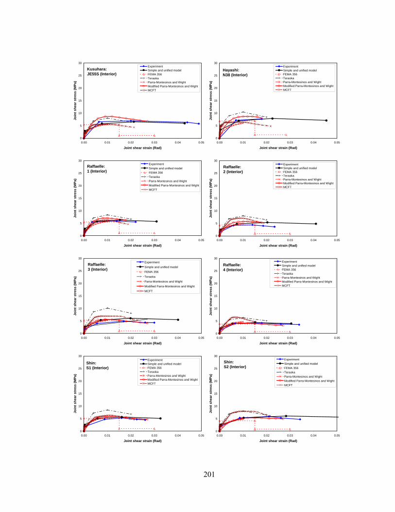
201

0

5

10

15

20

25

30

0.00 0.01 0.02 0.03 0.04 0.05

Joint shear strain (Rad)

Join

t she

ar s

tres

s (M

Pa)

ExperimentSimple and unified modelFEMA 356TeraokaParra-Montesinos and WightModified Parra-Montesinos and WightMCFT

Kusuhara: JE55S (Interior)

0

5

10

15

20

25

30

0.00 0.01 0.02 0.03 0.04 0.05

Joint shear strain (Rad)

Join

t she

ar s

tres

s (M

Pa)

ExperimentSimple and unified modelFEMA 356TeraokaParra-Montesinos and WightModified Parra-Montesinos and WightMCFT

Hayashi: N38 (Interior)

0

5

10

15

20

25

30

0.00 0.01 0.02 0.03 0.04 0.05

Joint shear strain (Rad)

Join

t she

ar s

tres

s (M

Pa)

ExperimentSimple and unified modelFEMA 356TeraokaParra-Montesinos and WightModified Parra-Montesinos and WightMCFT

Raffaelle: 1 (Interior)

0

5

10

15

20

25

30

0.00 0.01 0.02 0.03 0.04 0.05

Joint shear strain (Rad)

Join

t she

ar s

tres

s (M

Pa)

ExperimentSimple and unified modelFEMA 356TeraokaParra-Montesinos and WightModified Parra-Montesinos and WightMCFT

Raffaelle: 2 (Interior)

0

5

10

15

20

25

30

0.00 0.01 0.02 0.03 0.04 0.05

Joint shear strain (Rad)

Join

t she

ar s

tres

s (M

Pa)

ExperimentSimple and unified modelFEMA 356TeraokaParra-Montesinos and WightModified Parra-Montesinos and WightMCFT

Raffaelle: 3 (Interior)

0

5

10

15

20

25

30

0.00 0.01 0.02 0.03 0.04 0.05

Joint shear strain (Rad)

Join

t she

ar s

tres

s (M

Pa)

ExperimentSimple and unified modelFEMA 356TeraokaParra-Montesinos and WightModified Parra-Montesinos and WightMCFT

Raffaelle: 4 (Interior)

0

5

10

15

20

25

30

0.00 0.01 0.02 0.03 0.04 0.05

Joint shear strain (Rad)

Join

t she

ar s

tres

s (M

Pa)

ExperimentSimple and unified modelFEMA 356TeraokaParra-Montesinos and WightModified Parra-Montesinos and WightMCFT

Shin: S1 (Interior)

0

5

10

15

20

25

30

0.00 0.01 0.02 0.03 0.04 0.05

Joint shear strain (Rad)

Join

t she

ar s

tres

s (M

Pa)

ExperimentSimple and unified modelFEMA 356TeraokaParra-Montesinos and WightModified Parra-Montesinos and WightMCFT

Shin: S2 (Interior)

202

Subassembly conditions: Below 0.70 in Ash ratio; No out-of-plane; and No joint eccentricity

0

5

10

15

20

25

30

0.00 0.01 0.02 0.03 0.04 0.05

Joint shear strain (Rad)

Join

t she

ar s

tres

s (M

Pa)

ExperimentSimple and unified modelFEMA 356TeraokaModified Parra-Montesinos and WightMCFT

Meinheit: 6 (Interior)

0

5

10

15

20

25

30

0.00 0.01 0.02 0.03 0.04 0.05

Joint shear strain (Rad)

Join

t she

ar s

tres

s (M

Pa)

ExperimentSimple and unified modelFEMA 356TeraokaModified Parra-Montesinos and WightMCFT

Noguchi: No 2 (Interior)

0

5

10

15

20

25

30

0.00 0.01 0.02 0.03 0.04 0.05

Joint shear strain (Rad)

Join

t she

ar s

tres

s (M

Pa)

ExperimentSimple and unified modelFEMA 356TeraokaModified Parra-Montesinos and WightMCFT

Noguchi: No 4 (Interior)

0

5

10

15

20

25

30

0.00 0.01 0.02 0.03 0.04 0.05

Joint shear strain (Rad)

Join

t she

ar s

tres

s (M

Pa)

ExperimentSimple and unified modelFEMA 356TeraokaModified Parra-Montesinos and WightMCFT

Endoh: HC (Interior)

0

5

10

15

20

25

30

0.00 0.01 0.02 0.03 0.04 0.05

Joint shear strain (Rad)

Join

t she

ar s

tres

s (M

Pa)

ExperimentSimple and unified modelFEMA 356TeraokaModified Parra-Montesinos and WightMCFT

Joh: B1 (Interior)

0

5

10

15

20

25

30

0.00 0.01 0.02 0.03 0.04 0.05

Joint shear strain (Rad)

Join

t she

ar s

tres

s (M

Pa)

ExperimentSimple and unified modelFEMA 356TeraokaModified Parra-Montesinos and WightMCFT

Kitayama: I3 (Interior)

0

5

10

15

20

25

30

0.00 0.01 0.02 0.03 0.04 0.05

Joint shear strain (Rad)

Join

t she

ar s

tres

s (M

Pa)

ExperimentSimple and unified modelFEMA 356TeraokaModified Parra-Montesinos and WightMCFT

Goto: PL (Interior)

0

5

10

15

20

25

30

0.00 0.01 0.02 0.03 0.04 0.05

Joint shear strain (Rad)

Join

t she

ar s

tres

s (M

Pa)

ExperimentSimple and unified modelFEMATeraokaModified Parra-Montesinos and WightMCFT

Teraoka: HNO5 (Interior)

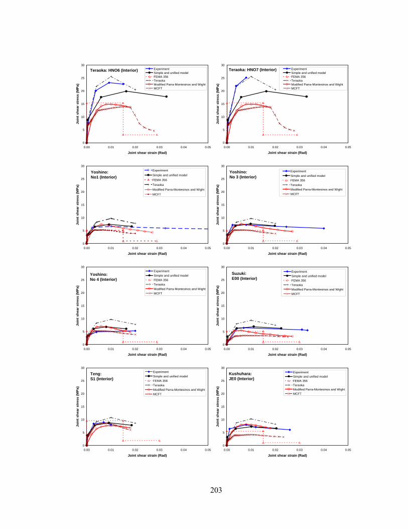
203

0

5

10

15

20

25

30

0.00 0.01 0.02 0.03 0.04 0.05

Joint shear strain (Rad)

Join

t she

ar s

tres

s (M

Pa)

ExperimentSimple and unified modelFEMA 356TeraokaModified Parra-Montesinos and WightMCFT

Teraoka: HNO6 (Interior)

0

5

10

15

20

25

30

0.00 0.01 0.02 0.03 0.04 0.05

Joint shear strain (Rad)

Join

t she

ar s

tres

s (M

Pa)

ExperimentSimple and unified modelFEMA 356TeraokaModified Parra-Montesinos and WightMCFT

Teraoka: HNO7 (Interior)

0

5

10

15

20

25

30

0.00 0.01 0.02 0.03 0.04 0.05

Joint shear strain (Rad)

Join

t she

ar s

tres

s (M

Pa)

ExperimentSimple and unified modelFEMA 356TeraokaModified Parra-Montesinos and WightMCFT

Yoshino: No1 (Interior)

0

5

10

15

20

25

30

0.00 0.01 0.02 0.03 0.04 0.05

Joint shear strain (Rad)

Join

t she

ar s

tres

s (M

Pa)

ExperimentSimple and unified modelFEMA 356TeraokaModified Parra-Montesinos and WightMCFT

Yoshino: No 3 (Interior)

0

5

10

15

20

25

30

0.00 0.01 0.02 0.03 0.04 0.05

Joint shear strain (Rad)

Join

t she

ar s

tres

s (M

Pa)

ExperimentSimple and unified modelFEMA 356TeraokaModified Parra-Montesinos and WightMCFT

Yoshino: No 4 (Interior)

0

5

10

15

20

25

30

0.00 0.01 0.02 0.03 0.04 0.05

Joint shear strain (Rad)

Join

t she

ar s

tres

s (M

Pa)

ExperimentSimple and unified modelFEMA 356TeraokaModified Parra-Montesinos and WightMCFT

Suzuki: E00 (Interior)

0

5

10

15

20

25

30

0.00 0.01 0.02 0.03 0.04 0.05

Joint shear strain (Rad)

Join

t she

ar s

tres

s (M

Pa)

ExperimentSimple and unified modelFEMA 356TeraokaModified Parra-Montesinos and WightMCFT

Teng: S1 (Interior)

0

5

10

15

20

25

30

0.00 0.01 0.02 0.03 0.04 0.05

Joint shear strain (Rad)

Join

t she

ar s

tres

s (M

Pa)

ExperimentSimple and unified modelFEMA 356TeraokaModified Parra-Montesinos and WightMCFT

Kushuhara: JE0 (Interior)

204

0

5

10

15

20

25

30

0.00 0.01 0.02 0.03 0.04 0.05

Joint shear strain (Rad)

Join

t she

ar s

tres

s (M

Pa)

ExperimentSimple and unified modelFEMA 356TeraokaModified Parra-Montesinos and WightMCFT

Meinheit: 1 (Interior)

0

5

10

15

20

25

30

0.00 0.01 0.02 0.03 0.04 0.05

Joint shear strain (Rad)

Join

t she

ar s

tres

s (M

Pa)

ExperimentSimple and unified modelFEMA 356TeraokaModified Parra-Montesinos and WightMCFT

Meinheit: 2 (Interior)

0

5

10

15

20

25

30

0.00 0.01 0.02 0.03 0.04 0.05

Joint shear strain (Rad)

Join

t she

ar s

tres

s (M

Pa)

ExperimentSimple and unified modelFEMA 356TeraokaModified Parra-Montesinos and WightMCFT

Meinheit: 3 (Interior)

0

5

10

15

20

25

30

0.000 0.010 0.020 0.030 0.040 0.050 0.060

Joint shear strain (Rad)

Join

t she

ar s

tres

s (M

Pa)

ExperimentSimple and unified modelFEMA 356TeraokaModified Parra-Montesinos and WightMCFT

Meinheit: 4 (Interior)

0

5

10

15

20

25

30

0.00 0.01 0.02 0.03 0.04 0.05

Joint shear strain (Rad)

Join

t she

ar s

tres

s (M

Pa)

ExperimentSimple and unified modelFEMA 356TeraokaModified Parra-Montesinos and WightMCFT

Meinheit: 5 (Interior)

0

5

10

15

20

25

30

0.00 0.01 0.02 0.03 0.04 0.05

Joint shear strain (Rad)

Join

t she

ar s

tres

s (M

Pa)

ExperimentSimple and unified modelFEMA 356TeraokaModified Parra-Montesinos and WightMCFT

Meinheit: 7 (Interior)

0

5

10

15

20

25

30

0.00 0.01 0.02 0.03 0.04 0.05

Joint shear strain (Rad)

Join

t she

ar s

tres

s (M

Pa)

ExperimentSimple and unified modelFEMA 356TeraokaModified Parra-Montesinos and WightMCFT

Endoh: A1 (Interior)

0

5

10

15

20

25

30

0.00 0.01 0.02 0.03 0.04 0.05

Joint shear strain (Rad)

Join

t she

ar s

tres

s (M

Pa)

ExperimentSimple and unified modelFEMA 356TeraokaModified Parra-Montesinos and WightMCFT

Fujii: A1 (Interior)

205

0

5

10

15

20

25

30

0.00 0.01 0.02 0.03 0.04 0.05

Joint shear strain (Rad)

Join

t she

ar s

tres

s (M

Pa)

ExperimentSimple and unified modelFEMA 356TeraokaModified Parra-Montesinos and WightMCFT

Fujii: A2 (Interior)

0

5

10

15

20

25

30

0.00 0.01 0.02 0.03 0.04 0.05

Joint shear strain (Rad)

Join

t she

ar s

tres

s (M

Pa)

ExperimentSimple and unified modelFEMA 356TeraokaModified Parra-Montesinos and WightMCFT

Fujii: A3 (Interior)

0

5

10

15

20

25

30

0.00 0.01 0.02 0.03 0.04 0.05

Joint shear strain (Rad)

Join

t she

ar s

tres

s (M

Pa)

ExperimentSimple and unified modelFEMA 356TeraokaModified Parra-Montesinos and WightMCFT

Goto: UM0 (Interior)

0

5

10

15

20

25

30

0.00 0.01 0.02 0.03 0.04 0.05

Joint shear strain (Rad)

Join

t she

ar s

tres

s (M

Pa)

ExperimentSimple and unified modelFEMA 356TeraokaModified Parra-Montesinos and WightMCFT

Kaku: No 3 (Exterior)

0

5

10

15

20

25

30

0.000 0.010 0.020 0.030 0.040 0.050

Joint shear strain (Rad)

Join

t she

ar s

tres

s (M

Pa)

ExperimentSimple and unified modelFEMA 356TeraokaModified Parra-Montesinos and WightMCFT

Kaku: No 5 (Exterior)

0

5

10

15

20

25

30

0.00 0.01 0.02 0.03 0.04 0.05

Joint shear strain (Rad)

Join

t she

ar s

tres

s (M

Pa)

ExperimentSimple and unified modelFEMA 356TeraokaModified Parra-Montesinos and WightMCFT

Kaku: No6 (Exterior)

0

5

10

15

20

25

30

0.00 0.01 0.02 0.03 0.04 0.05

Joint shear strain (Rad)

Join

t she

ar s

tres

s (M

Pa)

ExperimentSimple and unified modelFEMA 356TeraokaModified Parra-Montesinos and WightMCFT

Kaku: No 9 (Exterior)

0

5

10

15

20

25

30

0.00 0.01 0.02 0.03 0.04 0.05

Joint shear strain (Rad)

Join

t she

ar s

tres

s (M

Pa)

ExperimentSimple and unified modelFEMA 356TeraokaModified Parra-Montesinos and WightMCFT

Kaku: No 11 (Exterior)

206

0

5

10

15

20

25

30

0.00 0.01 0.02 0.03 0.04 0.05

Joint shear strain (Rad)

Join

t she

ar s

tres

s (M

Pa)

ExperimentSimple and unified modelFEMA 356TeraokaModified Parra-Montesinos and WightMCFT

Kaku: No 12 (Exterior)

0

5

10

15

20

25

30

0.00 0.01 0.02 0.03 0.04 0.05

Joint shear strain (Rad)

Join

t she

ar s

tres

s (M

Pa)

ExperimentSimple and unified modelFEMA 356TeraokaModified Parra-Montesinos and WightMCFT

Kaku: No 14 (Exterior)

0

5

10

15

20

25

30

0.00 0.01 0.02 0.03 0.04 0.05

Joint shear strain (Rad)

Join

t she

ar s

tres

s (M

Pa)

ExperimentSimple and unified modelFEMA 356

TeraokaModified Parra-Montesinos and Wight

MCFT

Kaku: No 15 (Exterior)

0

5

10

15

20

25

30

0.00 0.01 0.02 0.03 0.04 0.05

Joint shear strain (Rad)

Join

t she

ar s

tres

s (M

Pa)

ExperimentSimple and unified modelFEMA 356TeraokaModified Parra-Montesinos and WightMCFT

Fujii: B2 (Exterior)

0

5

10

15

20

25

30

0.00 0.01 0.02 0.03 0.04 0.05

Joint shear strain (Rad)

Join

t she

ar s

tres

s (M

Pa)

ExperimentSimple and unified modelFEMA 356TeraokaModified Parra-Montesinos and WightMCFT

Joh: NRCJ-12

0

5

10

15

20

25

30

0.00 0.01 0.02 0.03 0.04 0.05

Joint shear strain (Rad)

Join

t she

ar s

tres

s (M

Pa)

ExperimentSimple and unified modelFEMA 356TeraokaModified Parra-Montesinos and WightMCFT

Joh: LO-NO (Exterior)

0

5

10

15

20

25

30

0.00 0.01 0.02 0.03 0.04 0.05

Joint shear strain (Rad)

Join

t she

ar s

tres

s (M

Pa)

ExperimentSimple and unified modelFEMA 356TeraokaModified Parra-Montesinos and WightMCFT

Joh: LO-N96 (Exterior)

0

5

10

15

20

25

30

0.00 0.01 0.02 0.03 0.04 0.05

Joint shear strain (Rad)

Join

t she

ar s

tres

s (M

Pa)

ExperimentSimple and unified modelFEMA 356TeraokaModified Parra-Montesinos and WightMCFT

kaku: N22 (Exterior)

207

0

5

10

15

20

25

30

0.00 0.01 0.02 0.03 0.04 0.05

Joint shear strain (Rad)

Join

t she

ar s

tres

s (M

Pa)

ExperimentSimple and unified modelFEMA 356TeraokaModified Parra-Montesinos and WightMCFT

Fujii: B1 (Exterior)

0

5

10

15

20

25

30

0.00 0.01 0.02 0.03 0.04 0.05

Joint shear strain (Rad)

Join

t she

ar s

tres

s (M

Pa)

ExperimentSimple and unified modelFEMA 356TeraokaModified Parra-Montesinos and WightMCFT

Fujii: B3 (Exterior)

0

5

10

15

20

25

30

0.00 0.01 0.02 0.03 0.04 0.05

Joint shear strain (Rad)

Join

t she

ar s

tres

s (M

Pa)

ExperimentSimple and unified modelFEMA 356TeraokaModified Parra-Montesinos and WightMCFT

Joh: NRC-J8 (Exterior)

0

5

10

15

20

25

30

0.00 0.01 0.02 0.03 0.04 0.05

Joint shear strain (Rad)

Join

t she

ar s

tres

s (M

Pa)

ExperimentSimple and unified modelFEMA 356TeraokaModified Parra-Montesinos and WightMCFT

Wallace: KJ9 (Knee)

0

5

10

15

20

25

30

0.00 0.01 0.02 0.03 0.04 0.05

Joint shear strain (Rad)

Join

t she

ar s

tres

s (M

Pa)

ExperimentSimple and unified modelFEMA 356TeraokaModified Parra-Montesinos and WightMCFT

Wallace: KJ 12 (Knee)

0

5

10

15

20

25

30

0.00 0.01 0.02 0.03 0.04 0.05

Joint shear strain (Rad)

Join

t she

ar s

tres

s (M

Pa)

ExperimentSimple and unified modelFEMA 356TeraokaModified Parra-Montesinos and WightMCFT

Tabata: LBH1 (Knee)

0

5

10

15

20

25

30

0.00 0.01 0.02 0.03 0.04 0.05

Joint shear strain (Rad)

Join

t she

ar s

tres

s (M

Pa)

ExperimentSimple and unified modelFEMA 356TeraokaModified Parra-Montesinos and WightMCFT

Tabata: LBH2 (Knee)

208

Subassembly conditions: Below 0.70 in Ash ratio; With out-of-plane; and No joint eccentricity

0

5

10

15

20

25

30

0.00 0.01 0.02 0.03 0.04 0.05

Joint shear strain (Rad)

Join

t she

ar s

tres

s (M

Pa)

ExperimentSimple and unified modelFEMA 356TeraokaModified Parra-Montesinos and WightMCFT

Suzuki: E00s (Interior)

0

5

10

15

20

25

30

0.00 0.01 0.02 0.03 0.04 0.05

Joint shear strain (Rad)

Join

t she

ar s

tres

s (M

Pa)

ExperimentSimple and unified modelFEMA 356TeraokaModified Parra-Montesinos and WightMCFT

Meinheit: 9 (Interior)

0

5

10

15

20

25

30

0.00 0.01 0.02 0.03 0.04 0.05

Joint shear strain (Rad)

Join

t she

ar s

tres

s (M

Pa)

ExperimentSimple and unified modelFEMA 356TeraokaModified Parra-Montesinos and WightMCFT

Meinheit: 10 (Interior)

0

5

10

15

20

25

30

0.00 0.01 0.02 0.03 0.04 0.05

Joint shear strain (Rad)

Join

t she

ar s

tres

s (M

Pa)

ExperimentSimple and unified modelFEMA 356TeraokaModified Parra-Montesinos and WightMCFT

Meinheit: 11 (Interior)

Subassembly conditions: Below 0.70 in Ash ratio; No out-of-plane; and With joint eccentricity

0

5

10

15

20

25

30

0.00 0.01 0.02 0.03 0.04 0.05

Joint shear strain (Rad)

Join

t she

ar s

tres

s (M

Pa)

ExperimentSimple and unified modelFEMA 356TeraokaModified Parra-Montesinos and WightMCFT

Goto: LM60 (Interior)

0

5

10

15

20

25

30

0.00 0.01 0.02 0.03 0.04 0.05

Joint shear strain (Rad)

Join

t she

ar s

tres

s (M

Pa)

ExperimentSimple and unified modelFEMA 356TeraokaModified Parra-Montesinos and WightMCFT

Goto: LM125 (Interior)

209

0

5

10

15

20

25

30

0.00 0.01 0.02 0.03 0.04 0.05

Joint shear strain (Rad)

Join

t she

ar s

tres

s (M

Pa)

ExperimentSimple and unified modelFEMA 356TeraokaModified Parra-Montesinos and WightMCFT

Goto: HM60 (Interior)

0

5

10

15

20

25

30

0.00 0.01 0.02 0.03 0.04 0.05

Joint shear strain (Rad)

Join

t she

ar s

tres

s (M

Pa)

ExperimentSimple and unified modelFEMA 356TeraokaModified Parra-Montesinos and WightMCFT

Kushuhara: JE55 (Interior)

0

5

10

15

20

25

30

0.00 0.01 0.02 0.03 0.04 0.05

Joint shear strain (Rad)

Join

t she

ar s

tres

s (M

Pa)

ExperimentSimple and unified modelFEMA 356TeraokaModified Parra-Montesinos and WightMCFT

Suzuki: E085 (Interior)

0

5

10

15

20

25

30

0.00 0.01 0.02 0.03 0.04 0.05

Joint shear strain (Rad)

Join

t she

ar s

tres

s (M

Pa)

ExperimentSimple and unified modelFEMA 356TeraokaModified Parra-Montesinos and WightMCFT

Suzuki: E135 (Interior)

0

5

10

15

20

25

30

0.00 0.01 0.02 0.03 0.04 0.05

Joint shear strain (Rad)

Join

t she

ar s

tres

s (M

Pa)

ExperimentSimple and unified modelFEMA 356TeraokaModified Parra-Montesinos and WightMCFT

Goto: UM60 (Interior)

0

5

10

15

20

25

30

0.00 0.01 0.02 0.03 0.04 0.05

Joint shear strain (Rad)

Join

t she

ar s

tres

s (M

Pa)

ExperimentSimple and unified modelFEMA 356TeraokaModified Parra-Montesinos and WightMCFT

Goto: UM125 (Interior)

0

5

10

15

20

25

30

0.00 0.01 0.02 0.03 0.04 0.05

Joint shear strain (Rad)

Join

t she

ar s

tres

s (M

Pa)

ExperimentSimple and unified modelFEMA 356TeraokaModified Parra-Montesinos and WightMCFT

Goto: UU125 (Interior)

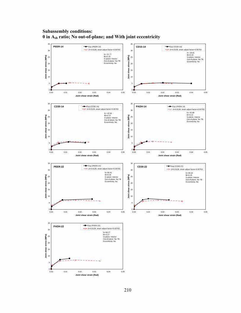
210

Subassembly conditions: 0 in Ash ratio; No out-of-plane; and With joint eccentricity

0

5

10

15

20

25

30

35

0.00 0.01 0.02 0.03 0.04 0.05

Joint shear strain (Rad)

Join

t she

ar s

tres

s (M

Pa)

Exp (PEER-14)JI=0.0128, strain adjust factor=0.00763

fc= 31.77BI=0.18In-plane: InteriorOut-of-plane: No TBEccentricity: No

PEER-14

0

5

10

15

20

25

30

35

0.00 0.01 0.02 0.03 0.04 0.05

Joint shear strain (Rad)

Join

t she

ar s

tres

s (M

Pa)

Exp (CD30-14)JI=0.0128, strain adjust factor=0.00763

fc= 29.81BI=0.19In-plane: InteriorOut-of-plane: No TBEccentricity: No

CD15-14

0

5

10

15

20

25

30

35

0.00 0.01 0.02 0.03 0.04 0.05

Joint shear strain (Rad)

Join

t she

ar s

tres

s (M

Pa)

Exp (CD30-14)JI=0.0128, strain adjust factor=0.00763

CD30-14

fc= 42.56BI=0.13In-plane: InteriorOut-of-plane: No TBEccentricity: No

0

5

10

15

20

25

30

35

0.00 0.01 0.02 0.03 0.04 0.05

Joint shear strain (Rad)

Join

t she

ar s

tres

s (M

Pa)

Exp (PADH-14)JI=0.0128, strain adjust factor=0.00763

fc= 42.88BI=0.13In-plane: InteriorOut-of-plane: No TBEccentricity: No

PADH-14

0

5

10

15

20

25

30

35

0.00 0.01 0.02 0.03 0.04 0.05

Joint shear strain (Rad)

Join

t she

ar s

tres

s (M

Pa)

Exp (PEER-22)JI=0.0128, strain adjust factor=0.00763

fc=38.41BI=0.26In-plane: InteriorOut-of-plane: No TBEccentricity: No

PEER-22

0

5

10

15

20

25

30

35

0.00 0.01 0.02 0.03 0.04 0.05

Joint shear strain (Rad)

Join

t she

ar s

tres

s (M

Pa)

Exp (CD30-22)JI=0.0128, strain adjust factor=0.00763

fc=38.16BI=0.25In-plane: InteriorOut-of-plane: No TBEccentricity: No

CD30-22

0

5

10

15

20

25

30

35

0.00 0.01 0.02 0.03 0.04 0.05

Joint shear strain (Rad)

Join

t she

ar s

tres

s (M

Pa)

Exp (PADH-22)JI=0.0128, strain adjust factor=0.00763

PADH-22

fc=36.27BI=0.27In-plane: InteriorOut-of-plane: No TBEccentricity: No

List of Recent NSEL Reports

No. Authors Title Date

004 Kwon, O-S. and Probabilistic Seismic Assessment of Structure, Foundation, Dec. 2007 Elnashai, A.S. and Soil Interacting Systems

005 Nakata, N., Multi-dimensional Mixed-mode Hybrid Simulation: Dec. 2007 Spencer, B.F., and Control and Applications Elnashai, A.S.

006 Carrion, J. and Model-based Strategies for Real-time Hybrid Testing Dec. 2007 Spencer, B.F.

007 Kim, Y.S., Seismic Loss Assessment and Mitigation for Critical Urban Jan. 2008 Spencer, B.F., and Infrastructure Systems Elnashai, A.S. 008 Gourley, B.C., Tort, C., A Synopsis of Studies of the Monotonic and Cyclic Behavior of April 2008 Denavit, M.D., Concrete-Filled Steel Tube Members, Connections, and Frames Schiller, P.H., and Hajjar, J.F. 009 Xu, D. and A New Node-to-node Approach to Contact/Impact Problems for May 2008 Hjelmstad, K.D. Two Dimensional Elastic Solids Subject to Finite Deformation 010 Zhu, J. and Non-contact NDT of Concrete Structures Using Air Coupled Sensors May 2008 Popovics, J.S. 011 Gao, Y. and Structural Health Monitoring Strategies for Smart Sensor Networks May 2008 Spencer, B.F. 012 Andrews, B., Performance-based Engineering Framework and Ductility Capacity July 2008 Fahnestock, L.A. and Models for Buckling-Restrained Braces Song, J. 013 Pallarés, L. and Headed Steel Stud Anchors in Composite Structures: Part I – Shear April 2009 Hajjar, J.F. 014 Pallarés, L. and Headed Steel Stud Anchors in Composite Structures: Part II – Tension April 2009 Hajjar, J.F. and Interaction 015 Walsh, S. and Data Processing of Laser Scans Towards Applications in June 2009 Hajjar, J.F. Structural Engineering 016 Reneckis, D. and Seismic Performance of Anchored Brick Veneer Aug. 2009 LaFave, J.M. 017 Borello, D.J., Behavior of Bolted Steel Slip-critical Connections with Fillers Aug. 2009 Denavit, M.D., and Hajjar, J.F. 018 Rice, J.A. and Flexible Smart Sensor Framework for Autonomous Full-scale Aug. 2009 Spencer, B.F. Structural Health Monitoring

019 Sim, S.-H. and Decentralized Strategies for Monitoring Structures using Nov. 2009 Spencer, B.F. Wireless Smart Sensor Networks 020 Kim, J. and Joint Shear Behavior of Reinforced Concrete Beam-Column Nov. 2009 LaFave, J.M. Connections subjected to Seismic Lateral Loading