Joint reconstruction of x-ray fluorescence andtransmission tomography

ZICHAO WENDY DI,1,2,* SI CHEN,2 YOUNG PYO HONG,3

CHRIS JACOBSEN,2,3,4 SVEN LEYFFER,1 AND STEFAN M. WILD1

1Mathematics and Computer Science Division, Argonne National Laboratory, 9700 South Cass Avenue,Lemont, IL 60439, USA2Advanced Photon Source, Argonne National Laboratory, 9700 South Cass Avenue, Lemont, IL 60439,USA3Department of Physics & Astronomy, Northwestern University, 2145 Sheridan Road, Evanston, IL60208, USA4Chemistry of Life Processes Institute, Northwestern University, 2170 Campus Drive, Evanston, IL60208, USA*wendydi@anl.gov

Abstract: X-ray fluorescence tomography is based on the detection of fluorescence x-ray pho-tons produced following x-ray absorption while a specimen is rotated; it provides informationon the 3D distribution of selected elements within a sample. One limitation in the quality ofsample recovery is the separation of elemental signals due to the finite energy resolution ofthe detector. Another limitation is the effect of self-absorption, which can lead to inaccurateresults with dense samples. To recover a higher quality elemental map, we combine x-ray flu-orescence detection with a second data modality: conventional x-ray transmission tomographyusing absorption. By using these combined signals in a nonlinear optimization-based approach,we demonstrate the benefit of our algorithm on real experimental data and obtain an improvedquantitative reconstruction of the spatial distribution of dominant elements in the sample. Com-pared with single-modality inversion based on x-ray fluorescence alone, this joint inversionapproach reduces ill-posedness and should result in improved elemental quantification and bet-ter correction of self-absorption.

c© 2017 Optical Society of America

OCIS codes: (340.7460) X-ray microscopy; (340.7440) X-ray imaging; (110.3010) Image reconstruction techniques;

(100.6950) Tomographic image processing.

References and links1. H. Moseley, “Atomic models and x-ray spectra,” Nature92, 554 (1914).2. C. J. Sparks, Jr., “X-ray fluorescence microprobe for chemical analysis,” in “Synchrotron Radiation Research,”

H. Winick and S. Doniach, eds. (Plenum Press, 1980), 459–512.3. J. Kirz, “Specimen damage considerations in biological microprobe analysis,” Scan Electron Microsc.2, 239–249

(1979).4. L. Grodzins, “Intrinsic and effective sensitivities of analysis by x-ray fluorescence induced by protons, electrons,

and photons,” Nucl. Instrum. Methods Phys. Res., Sect. A218, 203–208 (1983).5. V. Cosslett and P. Duncumb, “Micro-analysis by a flying-spot x-ray method,” Nature177, 1172–1173 (1956).6. P. Horowitz and J. A. Howell, “A scanning x-ray microscope using synchrotron radiation,” Science178, 608–611

(1972).7. C. G. Ryan, R. Kirkham, R. M. Hough, G. Moorhead, D. P. Siddons, M. D. de Jonge, D. J. Paterson, G. De Geron-

imo, D. L. Howard, and J. S. Cleverley, “Elemental x-ray imaging using the Maia detector array: The benefits andchallenges of large solid-angle,” Nucl. Instrum. Methods Phys. Res., Sect. A619, 37–43 (2010).

8. Y. Sun, S.-C. Gleber, C. Jacobsen, J. Kirz, and S. Vogt, “Optimizing detector geometry for trace element mappingby x-ray fluorescence,” Ultramicroscopy152, 44–56 (2015).

9. P. Boisseau and L. Grodzins, “Fluorescence tomography using synchrotron radiation at the NSLS,” Hyperfine Inter-act.33, 283–292 (1987).

10. R. Cesareo and S. Mascarenhas, “A new tomographic device based on the detection of fluorescent x-rays,” Nucl.Instrum. Methods Phys. Res., Sect. A277, 669–672 (1989).

11. M. D. de Jonge and S. Vogt, “Hard x-ray fluorescence tomography - an emerging tool for structural visualization,”Curr. Opin. Struct. Biol.20, 606–614 (2010).

Vol. 25, No. 12 | 12 Jun 2017 | OPTICS EXPRESS 13107

#292463 https://doi.org/10.1364/OE.25.013107 Journal © 2017 Received 19 Apr 2017; accepted 27 Apr 2017; published 30 May 2017

12. S. Vogt, “MAPS: A set of software tools for analysis and visualization of 3D x-ray fluorescence data sets,” J. Phys.IV 104, 635–638 (2003).

13. A. Muñoz-Barrutia, C. Pardo-Martin, T. Pengo, and C. Ortiz-de Solorzano, “Sparse algebraic reconstruction forfluorescence mediated tomography,” Proc. SPIE7446, 744604 (2009).

14. E. X. Miqueles and A. R. De Pierro, “Iterative reconstruction in x-ray fluorescence tomography based on Radoninversion,” IEEE Trans. Med. Imaging30, 438–450 (2011).

15. D. Gürsoy, T. Biçer, A. Lanzirotti, M. G. Newville, and F. De Carlo, “Hyperspectral image reconstruction for x-rayfluorescence tomography,” Opt. Express23, 9014–9023 (2015).

16. P. J. L. Rivière, P. Vargas, M. Newville, and S. R. Sutton, “Reduced-scan schemes for x-ray fluorescence computedtomography,” IEEE Trans. Nucl. Sci.54, 1535–1542 (2007).

17. L.-T. Chang, “A method for attenuation correction in radionuclide computed tomography,” IEEE Trans. Nucl. Sci.25, 638–643 (1978).

18. J. Nuyts, P. Dupont, S. Stroobants, R. Benninck, L. Mortelmans, and P. Suetens, “Simultaneous maximuma poste-riori reconstruction of attenuation and activity distributions from emission sinograms,” IEEE Trans. Med. Imaging18, 393–403 (1999).

19. H. Zaidi and B. Hasegawa, “Determination of the attenuation map in emission tomography,” J. Nucl. Medicine44,291–315 (2003).

20. J. P. Hogan, R. A. Gonsalves, and A. S. Krieger, “Fluorescent computer-tomography - a model for correction ofx-ray absorption,” IEEE Trans. Nucl. Sci.38, 1721–1727 (1991).

21. P. J. La Rivière, “Approximate analytic reconstruction in x-ray fluorescence computed tomography,” Phys. Med.Biol. 49, 2391–2405 (2004).

22. E. X. Miqueles and A. R. De Pierro, “Exact analytic reconstruction in x-ray fluorescence CT and approximatedversions,” Phys. Med. Biol.55, 1007–1024 (2010).

23. T. Yuasa, M. Akiba, T. Takeda, M. Kazama, A. Hoshino, Y. Watanabe, K. Hyodo, F. A. Dilmanian, T. Akatsuka, andY. Itai, “Reconstruction method for fluorescent x-ray computed tomography by least-squares method using singularvalue decomposition,” IEEE Trans. Nucl. Sci.44, 54–62 (1997).

24. Q. Yang, B. Deng, W. Lv, F. Shen, R. Chen, Y. Wang, G. Du, F. Yan, T. Xiao, and H. Xu, “Fast and accurate x-ray fluorescence computed tomography imaging with the ordered-subsets expectation maximization algorithm,” J.Synchrotron Radiat.19, 210–215 (2012).

25. C. G. Schroer, “Reconstructing x-ray fluorescence microtomograms,” Appl. Phys. Lett.79, 1912 (2001).26. P. J. La Rivière, D. Billmire, P. Vargas, M. Rivers, and S. R. Sutton, “Penalized-likelihood image reconstruction for

x-ray fluorescence computed tomography,” Opt. Eng.45, 077005 (2006).27. Q. Yang, B. Deng, G. Du, H. Xie, G. Zhou, T. Xiao, and H. Xu, “X-ray fluorescence computed tomography with

absorption correction for biomedical samples,” X-ray Spectrom.43, 278–285 (2014).28. B. Golosio, A. Simionovici, A. Somogyi, L. Lemelle, M. Chukalina, and A. Brunetti, “Internal elemental microanal-

ysis combining x-ray fluorescence, Compton and transmission tomography,” J. Appl. Phys.94, 145–156 (2003).29. B. Vekemans, L. Vincze, F. E. Brenker, and F. Adams, “Processing of three-dimensional microscopic x-ray fluores-

cence data,” J. Anal. At. Spectrom.19, 1302–1308 (2004).30. Z. Di, S. Leyffer, and S. M. Wild, “Optimization-based approach for joint x-ray fluorescence and transmission

tomographic inversion,” SIAM J. Imaging Sci.9, 1–23 (2016).31. A. C. Kak and M. Slaney,Principles of Computerized Tomographic Imaging (SIAM, 2001).32. J. Sherman, “The theoretical derivation of fluorescent x-ray intensities from mixtures,” Spectrochimica Acta7,

283–306 (1955).33. T. Schoonjans, A. Brunetti, B. Golosio, M. S. del Rio, V. A. Solé, C. Ferrero, and L. Vincze, “The xraylib library

for x-ray-matter interactions. Recent developments,” Spectrochim. Acta, Part B66, 776–784 (2011).34. W. T. Elam, B. D. Ravel, and J. R. Sieber, “A new atomic database for x-ray spectroscopic calculations,” Radiat.

Phys. Chem.63, 121–128 (2002).35. J. A. Browne and T. J. Holmes, “Developments with maximum-likelihood x-ray computed tomography: initial

testing with real data,” Appl. Opt.33, 3010–3022 (1994).36. T. J. Holmes and Y.-H. Liu, “Acceleration of maximum-likelihood image restoration for fluorescence microscopy

and other noncoherent imagery,” J. Opt. Soc. Am. A8, 893–907 (1991).37. S. G. Nash, “A survey of truncated-Newton methods,” J. Comput. Appl. Math.124, 45–59 (2000).38. F. De Carlo, D. Gürsoy, F. Marone, M. Rivers, D. Y. Parkinson, F. Khan, N. Schwarz, D. J. Vine, S. Vogt, S.-C.

Gleber, S. Narayanan, M. Newville, T. Lanzirotti, Y. Sun, Y. P. Hong, and C. Jacobsen, “Scientific Data Exchange:a schema for HDF5-based storage of raw and analyzed data,” J. Synchrotron Radiat.21, 1224–1230 (2014).

39. B. Hornberger, M. D. de Jonge, M. Feser, P. Holl, C. Holzner, C. Jacobsen, D. Legnini, D. Paterson, P. Rehak,L. Strüder, and S. Vogt, “Differential phase contrast with a segmented detector in a scanning x-ray microprobe,” J.Synchrotron Radiat.15, 355–362 (2008).

40. D. Gürsoy, F. De Carlo, X. Xiao, and C. Jacobsen, “TomoPy: a framework for the analysis of synchrotron tomo-graphic data,” J. Synchrotron Radiat.21, 1188–1193 (2014).

41. P. C. Hansen and D. P. O’Leary, “The use of the L-curve in the regularization of discrete ill-posed problems,” SIAMJ. Sci. Comput.14, 1487–1503 (1993).

42. S. G. Nash, “A multigrid approach to discretized optimization problems,” Opt. Meth. Softw.14, 99–116 (2000).

Vol. 25, No. 12 | 12 Jun 2017 | OPTICS EXPRESS 13108

1. Introduction

The use of characteristic x-ray emission lines to distinguish between different chemical ele-ments in a specimen goes back to the birth of quantum mechanics [1]. X-ray fluorescence canbe stimulated by energy transfer from electron or proton beams, but the best combination ofsensitivity and minimum radiation damage is provided by using x-ray absorption [2–4] for thispurpose. This is usually done in a scanning microscope mode, where a small x-ray beam spotis raster-scanned across the specimen while x-ray photons are collected by an energy disper-sive detector that provides a measure of the energy of each emitted photon [5]. Following earlydemonstrations [6], x-ray fluorescence microscopy is now commonplace in many laboratoriesand in particular at a wide range of synchrotron radiation light source facilities worldwide. Be-cause the x-ray beam from synchrotron light sources is usually linearly polarized in the horizon-tal direction, the energy dispersive detector is usually located at a position 90 in the horizontalfrom the incident beam so as to be centered on the direction of minimum elastic scattering asshown in Fig. 1 (other energy dispersive detector positions can be used [7], with various relativemerits [8]). Because the depth of focus of the x-ray beam is usually large compared to the spec-imen size, one can treat the incident x-ray beam as a pencil beam of constant diameter and thustranslate and rotate the specimen to obtain a set of 2D projections from each x-ray fluorescenceline for tomographic reconstruction [9,10], even for elements present at low concentration suchas trace elements in biological specimens [11].

Rotation angle θ

Incident x-ray

beam

XR

F d

ete

cto

r

(energ

y d

ispers

ive)

Pixel

XRT detector

Fig. 1. Top view of the geometry used in x-ray fluorescence microscopy. The x-ray beam is treated as a pencil beam in thez direction that is raster-scanned acrossthe specimen in 1D in thex direction, and the specimen is then rotated before an-other image is acquired (successive 2D planes are imaged by motion of the 3Dspecimen in they direction, into/out of the plane of this top view). The x-ray trans-mission signal (absorption) is recorded, and the x-ray fluorescence (XRF) signalis recorded over an angular range ofΩv by using an energy dispersive detectorlocated at 90 to the beam, in the direction of the elastic scattering minimumfor a horizontally polarized x-ray beam. The grid overlay on the specimen showsits discretization with a pixel size ofLv ; the set of pixels (in 2D; voxels in 3D)through which the XRF signal might undergo self-absorption in the specimen isindicated in orange.

A common approach is to collect the photon counts within predetermined energy windows, orto use per-pixel spectral fitting [12], so as to get immediate elemental concentration maps. Thesemaps are then used in conventional tomographic reconstruction schemes, such as filtered backprojection and iterative reconstruction techniques [13, 14]. A more recent approach has beento use a penalized maximum likelihood estimation method on the per-pixel spectra recordedby the energy dispersive detector for improved quantification and elemental separation [15];

Vol. 25, No. 12 | 12 Jun 2017 | OPTICS EXPRESS 13109

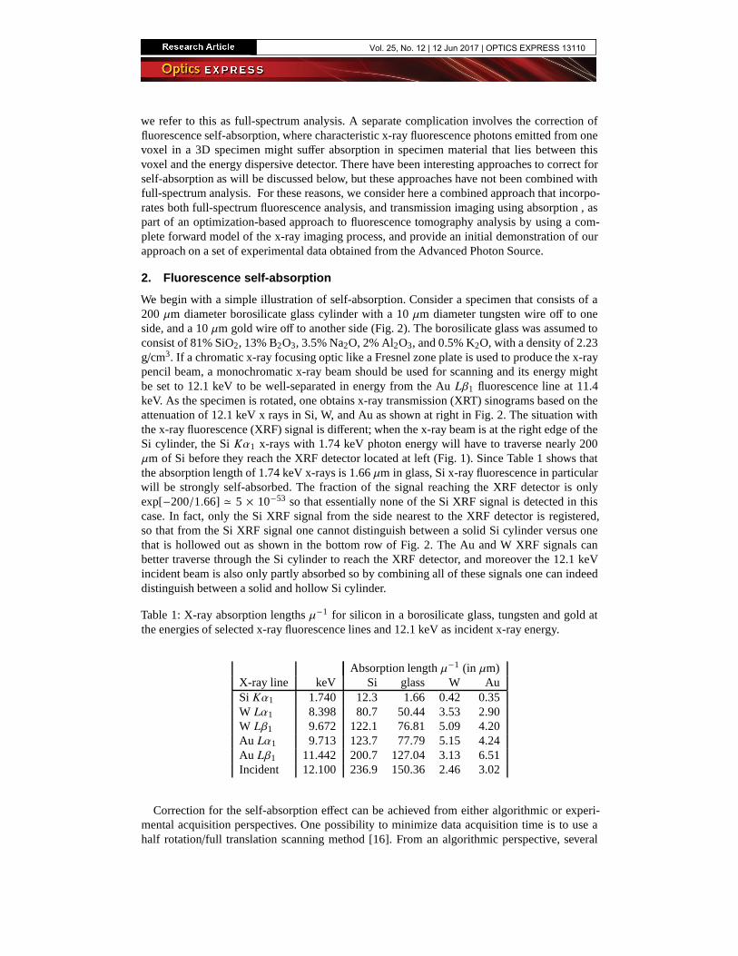
we refer to this as full-spectrum analysis. A separate complication involves the correction offluorescence self-absorption, where characteristic x-ray fluorescence photons emitted from onevoxel in a 3D specimen might suffer absorption in specimen material that lies between thisvoxel and the energy dispersive detector. There have been interesting approaches to correct forself-absorption as will be discussed below, but these approaches have not been combined withfull-spectrum analysis. For these reasons, we consider here a combined approach that incorpo-rates both full-spectrum fluorescence analysis, and transmission imaging using absorption , aspart of an optimization-based approach to fluorescence tomography analysis by using a com-plete forward model of the x-ray imaging process, and provide an initial demonstration of ourapproach on a set of experimental data obtained from the Advanced Photon Source.

2. Fluorescence self-absorption

We begin with a simple illustration of self-absorption. Consider a specimen that consists of a200 µm diameter borosilicate glass cylinder with a 10µm diameter tungsten wire off to oneside, and a 10µm gold wire off to another side (Fig. 2). The borosilicate glass was assumed toconsist of 81% SiO2, 13% B2O3, 3.5% Na2O, 2% Al2O3, and 0.5% K2O, with a density of 2.23g/cm3. If a chromatic x-ray focusing optic like a Fresnel zone plate is used to produce the x-raypencil beam, a monochromatic x-ray beam should be used for scanning and its energy mightbe set to 12.1 keV to be well-separated in energy from the AuLβ1 fluorescence line at 11.4keV. As the specimen is rotated, one obtains x-ray transmission (XRT) sinograms based on theattenuation of 12.1 keV x rays in Si, W, and Au as shown at right in Fig. 2. The situation withthe x-ray fluorescence (XRF) signal is different; when the x-ray beam is at the right edge of theSi cylinder, the SiKα1 x-rays with 1.74 keV photon energy will have to traverse nearly 200µm of Si before they reach the XRF detector located at left (Fig. 1). Since Table 1 shows thatthe absorption length of 1.74 keV x-rays is 1.66µm in glass, Si x-ray fluorescence in particularwill be strongly self-absorbed. The fraction of the signal reaching the XRF detector is onlyexp[−200/1.66] ≃ 5 × 10−53 so that essentially none of the Si XRF signal is detected in thiscase. In fact, only the Si XRF signal from the side nearest to the XRF detector is registered,so that from the Si XRF signal one cannot distinguish between a solid Si cylinder versus onethat is hollowed out as shown in the bottom row of Fig. 2. The Au and W XRF signals canbetter traverse through the Si cylinder to reach the XRF detector, and moreover the 12.1 keVincident beam is also only partly absorbed so by combining all of these signals one can indeeddistinguish between a solid and hollow Si cylinder.

Table 1: X-ray absorption lengthsµ−1 for silicon in a borosilicate glass, tungsten and gold atthe energies of selected x-ray fluorescence lines and 12.1 keV as incident x-ray energy.

Absorption lengthµ−1 (in µm)X-ray line keV Si glass W AuSi Kα1 1.740 12.3 1.66 0.42 0.35W Lα1 8.398 80.7 50.44 3.53 2.90W Lβ1 9.672 122.1 76.81 5.09 4.20Au Lα1 9.713 123.7 77.79 5.15 4.24Au Lβ1 11.442 200.7 127.04 3.13 6.51Incident 12.100 236.9 150.36 2.46 3.02

Correction for the self-absorption effect can be achieved from either algorithmic or experi-mental acquisition perspectives. One possibility to minimize data acquisition time is to use ahalf rotation/full translation scanning method [16]. From an algorithmic perspective, several

Vol. 25, No. 12 | 12 Jun 2017 | OPTICS EXPRESS 13110

methods have been used to correct for the self-absorption effect, including earlier approachesused for radionuclide emission tomography [17–19]. If one can measure the transmission sino-grams of the specimen at the energies of all x-ray fluorescence lines, it is possible to correctfor self absorption [20]. However, this approach is exceedingly difficult to realize experimen-tally, since a large number of x-ray fluorescence lines are present in many specimens and onewould need to collect a transmission tomography dataset at each of these energies. In the caseof uniform absorption and illumination at a single x-ray energy, analytical approaches havebeen developed [21, 22] and these have been shown [14] to provide a good starting point forthe iterative methods we now describe. One approach is to use algebraic (rather than filteredback projection) reconstruction methods to better handle limited rotational sampling, and least-squares fitting to better handle quantum noise [23]; other approaches have used ordered-subsetsexpectation maximization [24]. In more recent work, optimization approaches have been intro-duced where the transmission tomography data at a single x-ray energy was used to estimate theabsorption at all x-ray fluorescence energies using the fact that (in the absence of x-ray absorp-tion edges) x-ray absorption scales in a power-law relationship with x-ray energy [25–27]. Onecan also add the Compton scattered signal as another measurement of overall specimen electrondensity, and use the tabulated absorption coefficientsµEe of all elementse at each fluorescenceenergyE [28]. Other approaches classify the specimen as being composed of a finite numberof material phases for the calculation of self-absorption [29]. The optimization approaches inparticular serve as inspiration for our approach, which we believe is unique in combining bothfull-spectrum analysis and transmission imaging along with fluorescence.

We begin by briefly describing the mathematical “forward models” of XRF and XRT. Next,we detail our joint reconstruction approach and the formulation of the objective function andcorresponding optimization algorithm. We then discuss choices of scaling parameters in thenumerical implementation of the algorithm and present the performance of our joint inversioncompared with existing approaches on real datasets.

3. Mathematical model

We start from an earlier approach [30], which we extend considerably here to include a differentmodel of XRF self-absorption effect and the ability to better balance differences in variability ofacquired data. We useθ ∈ Θ andτ ∈ T to denote, respectively, the index of the x-ray beam angleand discretized beamlet from a collection of|Θ| angles and|T | beamlets. The setV denotesthe collection of|V | spatial voxels used to discretize the reconstructed sample. ByL = [Lθ ,τv ],we denote the intersection lengths (in cm) of beamlet (θ, τ) with the voxelv ∈ V . We useE todenote the collection of|E | possible elements andµEe to denote the mass attenuation coefficient(in cm2g−1) of elemente at beam incident energyE. Our goal is to recoverWWW = [Wv ,e], theconcentration (in g cm−3) of elemente in voxelv.

Vol. 25, No. 12 | 12 Jun 2017 | OPTICS EXPRESS 13111

Ro

tatio

n θ

Solid cylinder

without

self-absorption

Solid cylinder

with

self-absorption

Hollow cylinder

with

self-absorption

50 μm

Glass

AuW

Sample Sinogram from Si XRF Sinogram from XRT

Position τ Position τ

0

2

4

6

8

x10-3

3

4

x10-3

123456×1010

123456×1010

123456×1010

0

1

2

3

4

×10-3

0

1

2

Ro

tatio

n θ

Fig. 2. Illustration of the x-ray fluorescence self-absorption effect, and how x-raytransmission can be used to recognize and correct for it. We show here a specimencomposed of cylinders, or circles in this top view. The largest is of borosilicateglass (composition described in Sec. 2) with 200µm diameter, followed by tung-sten (W) with 10µm diameter, and gold (Au) with 10µm diameter. As 1D scansin beamlet positionsτ are collected at successive specimen rotation anglesθ, onebuilds up sinograms or (τ, θ) views of elemental x-ray fluorescence (XRF) signalssuch as the Si XRF signal shown in the middle, as well as 12.1 keV x-ray transmis-sion (XRT) sinograms as shown at right (based on absorption contrast). If there isno self-absorption of the fluorescence signal, one obtains a Si XRF sinogram asshown in the top row, where the incident x-ray beam is partially absorbed in thesmall W and Au wires as they rotate into positions to intercept the incident beambefore it reaches the glass cylinder. However, the 200µm diameter glass cylinderis large compared to the 1.66µm absorption lengthµ−1 of Si Kα1 x-rays in theglass as shown in Table 1, so that a fraction 1− exp[−200/1.66]≃ 1− 5 × 10−53

of the Si XRF signal will be self-absorbed in the rod. As a result, the Si XRFsignal will be detected mainly when the incident beam is at the left side of thescan; this leads to the Si XRF sinogram shown in the middle row (the sinogramalso shows absorption of the Si XRF signal in the W and Au wires as they rotatethrough positions where they partly obscure the XRF detector’s view of the Sicylinder). In the bottom row we show the case where the glass cylinder is hollow,with a wall thickness of 30µm that is nevertheless large compared to the 1.66µmabsorption length of Si XRF photons; in this case the Si XRF sinogram is almostunchanged, but the XRT sinogram is clearly different. By using the combinedinformation of the fluorescence (XRF) and transmission (XRT) sinograms, onecan in principle obtain a better reconstructed image of the specimen in the caseof strong fluorescence self-absorption.

Vol. 25, No. 12 | 12 Jun 2017 | OPTICS EXPRESS 13112

3.1. XRT imaging model

A conventional way (see, e.g., [31]) to model the XRT projectionFTθ ,τ

(in counts/sec) of asample from beamlet (θ, τ) is

FTθ ,τ(µµµE ) = I0 exp

−∑

v

Lθ ,τv µEv

, (1)

whereI0 is the incident x-ray intensity (in counts/sec) andµµµE = [ µEv ] is the linear attenuationabsorption coefficient (in cm−1) at incident energyE.

To better explore the correlation of XRF and XRT and to link these two data modalities bythe common variableWWW , we note that the coefficientsµµµE depend onWWW by way of µEv =∑

eWv ,eµ

Ee . Incorporating this fact in Eq. (1), we obtain a new XRT forward model based on

WWW

FTθ ,τ(WWW) = I0 exp

−∑

v ,e

Lθ ,τv µEeWv ,e

. (2)

To obtain a simple proportional relationship, we divide both sides of Eq. (2) byI0 and then takethe logarithm to obtain the XRT forward model used in this work:

FTθ ,τ(WWW) =

∑

v ,e

Lθ ,τv µEeWv ,e .

We similarly take the logarithm of the raw XRT sinograms used in this paper.

3.2. XRF imaging model

Our discrete model follows an elemental approach, in the sense that we model the XRF energyemitted from a single elemental atom by its corresponding elemental unit spectrum. We first ap-ply spectral blurring to each unit spectrum according to the detector’s response function. Then,justified by the fact that photon counts are additive, the total XRF spectrum detected from thegiven specimen model comes in after which is estimated as a weighted sum of the unit spectraof the elements being recovered.

First, we model the net XRF intensityIe ,ℓ ,s, which corresponds to the characteristic XRFenergyEe emitted from elemente, by Sherman’s equation [32] up to first order (i.e., neglectingeffects such as Rayleigh and Compton scattering):

Ie ,ℓ ,s = I0ceωe ,ℓ

(

1− 1re ,s

)

µEe , (3)

wherece is the total concentration of elemente (ce = 1 in the case of our unit spectra),ωe ,ℓ

is the XRF yield ofe for the spectral lineℓ, andre ,s is the probability that a shells electron(rather than other shell electrons) will be ejected.

In our calculations, the quantityωe ,ℓ

(

1− 1re ,s

)

µEe is approximated by the XRF cross sec-tions provided from xraylib [33]. Next, we convert the intensity to a spectrum by incorporatingthe practical experimental environment. Given an energy-dispersive XRF detector with energychannelsxi , i = 1, . . . , |I|, we define an indicator function

[1xEe

] i :=

1 if |xi − Ee | = minj

(|x j − Ee |) and xi , 2Ee − xi−1

0 otherwise.(4)

Then we have the ideal, delta-function peakIxe ,l ,s

= Ie ,l ,s1xEe

. In practice, because of the de-tector energy resolution [2], discrete x-ray lines get broadened by a Gaussian distribution with a

Vol. 25, No. 12 | 12 Jun 2017 | OPTICS EXPRESS 13113

standard deviationσ. The resulting unit spectrum of elemente is thus given byMe =∑

ℓ ,s

Me ,ℓ ,s,

where

Me ,ℓ ,s = F −1(

F (Ixe ,l ,s) ⊙ F

(

1√

2πσexp

−x2

2σ2

))

(5)

and where⊙ denotes pointwise (Hadamard product) multiplication andF (F −1) is the (inverse)Fourier transform. To simplify the model, we consider only theKα , Kβ , Lα , Lβ , andMα linesas tabulated [34].

We then model the total XRF spectrum of a sample with multiple elements by explicitlyconsidering the attenuation of the beam energy and the self-absorption effect of the XRF energy.We represent the attenuation experienced by beamlet (θ, τ) (at incident beam energyE) as ittravels toward voxelv by

AE ,θ ,τv (WWW) = exp

−∑

v′µEv′Lθ ,τv′

Iv′∈U

θ ,τv

= exp

−∑

v′

∑

eWv′ ,eµ

Ee L

θ ,τv′

Iv′∈U

θ ,τv

, (6)

whereIX is the indicator (Dirac delta) function for the eventX andUθ ,τv is the set of voxels

that are intersected by beamlet (θ, τ) before it enters voxelv.We let Pθ ,τ

v ,e(WWW) be the attenuation of XRF energy emitted from elemente at voxel v bybeamlet (θ, τ). To reduce the complexity of the calculation, instead of tracking all the emittedphotons isotropically, we consider only the emission from the regionΩv. This region is the partof the sample discretization that intersects the pyramid determined by the centroid of the voxelv and the XRF detector endpoints; see Fig. 1 for a 2D illustration. In a slight abuse of notation,we let v′′ ∈ Ωv indicate that the centroid of voxelv′′ is contained in the regionΩv. Then theself-absorbed XRF energy is approximated by

Pθ ,τv ,e(WWW) = exp

−∑

v′∈Ωv

∑

e′

Wv′ ,e′µEe

e′a(Ωv)

|v′′ : v′′ ∈ Ωv |

, (7)

wherea(Ω) is the volume ofΩ (or area ofΩ for a 2D sample) andµEe

e′is the linear attenuation

coefficient of elemente′ at the XRF energyEe of elemente. Accordingly, the fluorescencespectrumFR

θ ,τ (in counts/sec) of the sample resulting from beamlet (θ, τ) is the|I |-dimensionalvector

FRθ ,τ(WWW) =

∑

e

∑

v

Lθ ,τv AE ,θ ,τv (WWW)Pθ ,τ

v ,e(WWW)Wv ,e

Me .

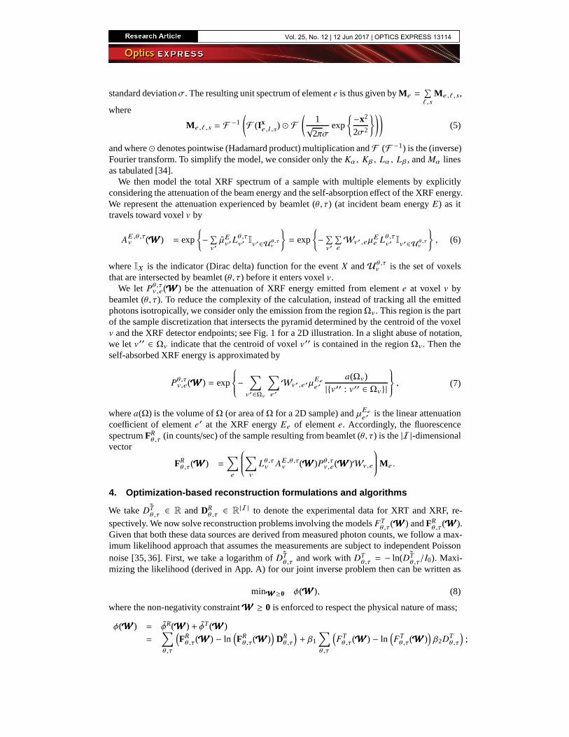
4. Optimization-based reconstruction formulations and algorithms

We take ˜DTθ ,τ∈ R andDR

θ ,τ∈ R

|I | to denote the experimental data for XRT and XRF, re-

spectively. We now solve reconstruction problems involving the modelsFTθ ,τ

(WWW) andFRθ ,τ

(WWW).Given that both these data sources are derived from measured photon counts, we follow a max-imum likelihood approach that assumes the measurements are subject to independent Poissonnoise [35, 36]. First, we take a logarithm ofDT

θ ,τand work withDT

θ ,τ= − ln( ˜DT

θ ,τ/I0). Maxi-

mizing the likelihood (derived in App. A) for our joint inverse problem then can be written as

minWWW≥0 φ(WWW), (8)

where the non-negativity constraintWWW ≥ 0 is enforced to respect the physical nature of mass;

φ(WWW) = φR(WWW) + φT (WWW)=

∑

θ ,τ

(

FRθ ,τ(WWW) − ln

(

FRθ ,τ(WWW)

)

DRθ ,τ

)

+ β1

∑

θ ,τ

(

FTθ ,τ(WWW) − ln

(

FTθ ,τ(WWW)

)

β2DTθ ,τ

)

;

Vol. 25, No. 12 | 12 Jun 2017 | OPTICS EXPRESS 13114

Algorithm 1 Algorithm for Solving Joint Inversion with Linearized XRF Term.

1: Given toleranceǫ > 0 and initialWWW0; initialize iteration counteri = 0.2: repeat3: [Ai ,PPPi ] = FR

θ ,τ(WWW i).

4: WWW i+1 = TN(φi(WWW),WWW i , 52).

5: Compute the search directionei =WWW i+1 −WWW i .6: Use backtracking line searchα = LIN_NAIVE( ei ,WWW i , φ, 1) (see Alg. 2) to obtainWWW i+1 =WWW i + αei.

7: i ← i + 1.8: until

∥

∥

∥WWW i+1 −WWW i∥

∥

∥ < ǫ

φR and φT correspond to the XRF and XRT objective terms, respectively; andβ1 ≥ 0, β2 ≥ 0are scaling parameters. The scaling parameterβ1 balances the ability of each modality to fit thedata, andβ2 detects the relative variability between the data sourcesDR

θ ,τandDT

θ ,τ.

Advances in x-ray sources, optics, and detectors mean that the datasets to be analyzed canbe large; thus, having a fast and memory-efficient algorithm to solve (8) is highly desirable.Therefore, we apply an alternating direction approach described in Alg. 1. In this approach,instead of directly minimizing Eq. (8), we first solve an “inner iteration” subproblem:

minWWW≥0 φi (WWW), (9)

withφi (WWW) =

∑

θ ,τ

∑

e ,v Lθ ,τv A

E ,θ ,τv (WWW i )Pθ ,τ

v ,e(WWW i )Wv ,eMe

−∑

θ ,τ ln(

∑

e ,v Lθ ,τv A

E ,θ ,τv (WWW i )Pθ ,τ

v ,e(WWW i )Wv ,eMe

)

DRθ ,τ

+ β1∑

θ ,τ

(

FTθ ,τ

(WWW) − ln(

FTθ ,τ

(WWW))

β2DTθ ,τ

)

,

and whereA(WWW i) andPPP(WWW i ) are fixed given the current solutionWWW i at the “outer” iterationiof Alg. 1.

To approximately solve Eq. (9), we adapt a form of the inexact truncated Newton (TN)method in [37]. We write TN as a function of the form

WWW i+1 = TN(φi(WWW),WWW i , k),

which appliesk iterations of TN to the problem in Eq. (9) with initial guessWWW i to obtainWWW i+1.In particular, we use a bound-constrained preconditioned conjugate gradient method to obtainthe search direction, followed by a backtracking line search (see Alg. 2) to obtain the next iterateWWW i+1. The process is repeated until desired stopping criteria are satisfied; in Alg. 1 we repeatuntil consecutive iterates are within a user-specified distanceǫ of one another. Since the focusof this work is to show the potential of joint inversion with multimodal data, future work willaddress convergence analysis of Alg. 1.

Algorithm 2 Backtracking Line Search

1: procedure α = lin_naive(d, x , f , αmax)2: repeat3: αmax← αmax

2 .4: until f (x + αmaxd) < f (x), thenα = αmax

5: end procedure

Vol. 25, No. 12 | 12 Jun 2017 | OPTICS EXPRESS 13115

Au

τθ

Si W

0 0.5 1

Fig. 3. Relative elemental concentrations obtained from a MAPS-based fit of theraw x-ray fluorescence data for the glass rod sample. Due to the imperfectionof fitting and background rejection (which might be able to be corrected withadditional expert input), the decomposed elemental concentrations show certainartifacts, where certain elemental sinograms pick up other elements’ signals. Forexample, according to our knowledge of the sample, we know that Si exists onlyin the rod part with a cylinder shape; but its corresponding sinogram shows thatit also exists in the two wires, which is caused by imperfect data fitting. Thosetwo extra curves in the sinogram are actually picked up from Au and W signalsbecause certain emission lines of Au and W overlap those of Si. Similar artifactshappen to Au and W sinograms as well.

5. Experimental reconstruction

We now demonstrate the benefit of the proposed joint inversion approach by using experimentaldata. We constructed a simple test sample consisting of a borosilica glass rod with a compositionas described in Sec. 2, wrapped with a W wire of 10µm diameter, and a Au wire of 10µmdiameter. This test specimen was scanned by an incident beam energy of 12.1 keV at beamline2-ID-E at the Advanced Photon Source at Argonne National Laboratory. Each projection wasacquired by raster scanning horizontally and vertically with a 200 nm scanning step size and 73scanning angles over an angular range of 360, with the data stored as HDF5 files with metadataincluded [38]. At each scanning step, the transmission signal was acquired using a four-segmentcharge-integrating silicon drift detector [39], while the fluorescence signals were collected byusing an energy-dispersive detector (Vortex ME-4) located at 90 relative to the incident beam,covering an energy range of 0–20 keV with 2,000 energy channels. We then sum the signalfrom the 4 transmission detector elements without distinguishing the fact that each elementsees a slightly different angle to obtain the final data; this results in 73 projections, with eachslice involving 1, 750× 51 pixels, and leads to a dataset of dimension 73× 1, 750× 51× 2, 000.

As expected from the attenuation lengths given in Table 1 and the simulations shown in Fig. 2,this dataset shows strong self-absorption in the Si fluorescence measurements. We compare ourreconstruction result with the output of TomoPy 0.1.15 [40], a widely used tomographic data-processing and image reconstruction library. TomoPy takes the elemental concentration mapdecomposed from the raw spectrum by the program MAPS 1.2 [12] for improved photon statis-tics compared with the raw data. The MAPS program fits the full energy spectrum recordedat each scan to a set of x-ray fluorescence peaks plus background signals, and it returns a 2Ddataset corresponding to a certain elemental concentration per scan. Figure 3 shows three el-emental XRF sinograms of interest as calculated by this approach. Within TomoPy, we useda maximum likelihood expectation maximization algorithm to reconstruct the three sinogramsseparately. All numerical experiments are performed on a platform with 1.5 TB DDR3 memoryand four Intel E7-4820 Xeon CPUs.

For the purposes of algorithm testing with reduced computational cost, we reconstructed onlya 2D middle slice (x , y) of the 3D glass rod dataset (x , y, z). For each angle, we summed together9 adjacenty slices of both XRF spectra and XRT measurements as the input experiment data.

Vol. 25, No. 12 | 12 Jun 2017 | OPTICS EXPRESS 13116

mean(DR)

τθ

0

5

10

15

DT

0

0.05

0.1

0.15

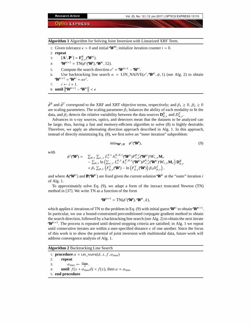
Fig. 4. Experimental sinograms. Left: mean (across energy channels) value ofXRF raw spectrum; Right: XRT optical density. Based on the different magni-tudes of these two datasets, we chooseβ2 = 100 as the scaling parameter to bal-ance the measurement variability of the two data sources, so that both measure-ments have maxima near 15 in their respective units. As a result, the relativevariability of the two detectors between the data sources is mitigated.

Furthermore, instead of using the full 2000 energy channels, we pick 40 energy channels aroundeach of the 20 emission lines provided by xraylib for each element’sKα , Kβ , Lα , Lβ , andMα

lines; this process returns a total of 800 energy channels to be considered in the reconstruction.Therefore, in our illustration,|θ | = 73, |τ | = 195, |E | = 800, and|V | = (|τ |) × (|τ |).

5.1. Selection of β values

Next, we explain one way to select values forβ1 and β2 for use in the objective in Eq. (8).We recall that the effect ofβ2 is to balance the magnitudes of the XRF and XRT measurementdata, and that its exact value is not critical. Therefore, according to the magnitude differenceof two data sources shown in Fig. 4, we chose to useβ2 = 100 to balance this difference sothat both measurements have maxima near 15 in their respective units. The selection ofβ1 isaccomplished by applying the so-called “L-curve method” [41]. In Fig. 5, we plot the L-curvedefined by the curve of XRT termsφT versus XRF termsφR obtained from solving Eq. (8)with differentβ1 values. This curve displays the tradeoffs between these two modalities andprovides an aid in choosing an appropriate balancing parameterβ1. The curvature, defined asthe curvature of a circle drawn through three successive points on the L-curve, is calculated andplotted in Fig. 6. As suggested by [41], we choose the point on the L-curve with the maximumcurvature; according to the objective values ofφR and φT shown in Fig. 5 and the curvatureshown in Fig. 6, this isβ1 = 1. Figure 10 shows the reconstructed elemental maps correspondingto differentβ1 values. For the two extreme casesβ1 = 0.001 andβ1 = 100, the reconstructionresults resemble the single-modality reconstructions. However, there is no significant differencebetween the results returned forβ1 ∈ [0.25, 10] based on our prior knowledge of the sample.This lack of sensitivity to precise balancing parameter values indicates robustness for practicalutilization.

5.2. Joint inversion results

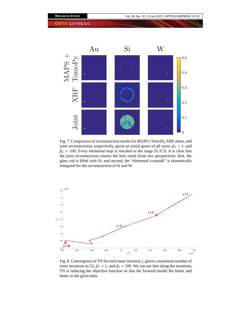
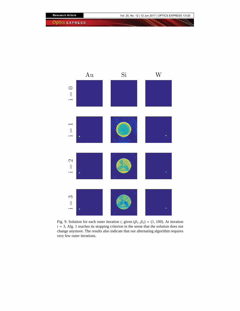
GivenWWW0 = 0 as the initial guess for the joint inversion, Fig. 7 shows the reconstruction resultfor each element by using Alg. 1 withǫ = 10−6. In particular, Fig. 8 shows the performance ofthe inner iteration by TN to reduce both the XRF and XRT objective values. Correspondingly,Fig. 9 shows the reconstructed result of each outer iteration of Alg. 1. The reconstructed elemen-tal maps show the benefits of our joint inversion mainly from two perspectives. First, becauseof the imperfections of spectral fitting and background rejection, the decomposed elementalconcentrations show certain artifacts—which we call the “elemental crosstalk ”—where certainelemental sinograms pick up other elements’ signals. For example, according to our knowledgeof the sample, we know that Si exists only in the rod part with a cylinder shape; but its corre-sponding sinogram from MAPS (Fig. 3) would suggest that it also exists in the two wires; this

Vol. 25, No. 12 | 12 Jun 2017 | OPTICS EXPRESS 13117

8.7 8.75 8.8 8.85 8.9 8.95 9

φR×10 5

-6

-5.5

-5

-4.5

-4

-3.5

φT

×10 4

β1

= 0

β1

= 0.001

β1

= 0.25

β1

= 0.5

β1

= 1

β1

= 2 β

1 = 4

β1

= 10 β

1 = 100 β

1 = ∞

Fig. 5. Method for choosing the parameterβ1 that appears in the cost function ofEq. (8): XRF objective valueφR versus XRT objective valueφT given differentvaluesβ1, with fixedβ2 = 100. The curve displays the tradeoff between these twomodalities.

0 10 20 30 40 50 60 70 80 90 100β1

0

0.2

0.4

0.6

0.8

1

1.2

1.4

Curvature

×10 -4

β1

= 1

Fig. 6. Method for choosing the parameterβ1 that appears in the cost function ofEq. (8): The curvature from successive points in Fig. 5; the point with maximumcurvature occurs atβ1 = 1.

is caused by imperfect data fitting. Those two extra curves in the sinogram are actually pickedup from Au and W signals because certain emission lines of Au and W overlap those of Si. As aresult, the reconstruction from TomoPy based on these decomposed sinograms will contain the“elemental-crosstalk points,” which are shown as two small dots around Si and a dot in the Wmap in the left bottom corner of Fig. 7. Comparing the results from XRF single inversion usingour forward model with the TomoPy output, we see that our forward model is able to betterdistinguish the different elemental signals; that is, the “elemental crosstalk” is greatly mitigated.Furthermore, by introducing the XRT modality into the reconstruction, the joint inversion notonly suppressed the artifacts from the “elemental crosstalk” introduced by the imperfect fittingand background rejection, but also more accurately recovered Si by filling the inside of thecylinder and thereby correcting the self-absorption effect. Also, we provide a quantity evalua-

Vol. 25, No. 12 | 12 Jun 2017 | OPTICS EXPRESS 13118

Au

MAPS+

Tom

oPy

Si W

XRF

Joint

0

0.1

0.2

0.3

0.4

0.5

Fig. 7. Comparison of reconstruction results for MAPS+TomoPy, XRF alone, andjoint reconstruction, respectively, given an initial guess of all zeros,β1 = 1, andβ2 = 100. Every elemental map is rescaled to the range [0, 0.5]. It is clear thatthe joint reconstruction returns the best result from two perspectives: first, theglass rod is filled with Si; and second, the “elemental crosstalk” is dramaticallymitigated for the reconstruction of Si and W.

8.2 8.4 8.6 8.8 9 9.2 9.4 9.6 9.8 10φR

×10 5

-6

-5

-4

-3

-2

-1

0

1

2

φT

×10 4

j = 52

j = 3

j = 2

j = 1

Fig. 8. Convergence of TN for each inner iterationj, given a maximum number ofinner iterations as 52,β1 = 1, andβ2 = 100. We can see that along the iterations,TN is reducing the objective function so that the forward model fits better andbetter to the given data.

Vol. 25, No. 12 | 12 Jun 2017 | OPTICS EXPRESS 13119

Aui=

0Si W

i=

1i=

2i=

3

Fig. 9. Solution for each outer iterationi, given (β1, β2) = (1, 100). At iterationi = 3, Alg. 1 reaches its stopping criterion in the sense that the solution does notchange anymore. The results also indicate that our alternating algorithm requiresvery few outer iterations.

Vol. 25, No. 12 | 12 Jun 2017 | OPTICS EXPRESS 13120

Au

β1=

0

Si W

β1=

0.00

1β

1=

1β

1=

4β

1=

10β

1=

100

β1=∞

Fig. 10. Reconstruction results (givenβ2 = 100) for differentβ1 values. Apartfrom the two extreme cases (β1 = 0.001, where XRF dominates, andβ1 = 100,where XRT dominates), the reconstructions do not show clear difference in termsof quality. Therefore, for a broad range ofβ1 values, the joint reconstruction isable to dramatically improve upon the single-modality reconstructions.

Vol. 25, No. 12 | 12 Jun 2017 | OPTICS EXPRESS 13121

tion of our reconstruction. We simulate the XRF spectrum based on the reconstructed elementalcomposition and compare it to the real experimental data as shown in Fig. 12. We can see that,except the background region that our forward model does not include to simulate, the essentialpeaks corresponding to the main elements we are interested to cover agree very well with theexperimental data. This comparison indicates that not only our joint reconstruction improvesthe solution from a visualization perspective, but also from quantification point of view. Fur-thermore, it indicates a satisfying accuracy of our XRF forward model.

One limitation of our method is the high requirement of computing resources for generatingthe forward mapping tensor incorporating the known mass attenuation coefficients. Overall,the reconstruction time spent on this particular test is 4301 seconds plus a couple of hours ongenerating the forward mapping. The main bottleneck is in the large memory requirement andthe calculation of the self-absorption term. Parallelizing our TN solver and projections/beamlets,or using multilevel schemes [42], would also accelerate the performance. This will be the focusof our future work.

6. Conclusion

Guided by the multimodal analysis methodology developed in [30], we apply a joint-inversionframework to solve XRF reconstruction problem more accurately by incorporating a seconddata modality as XRT. We investigate the correlations between XRF and XRT data, and estab-

0 2 4 6 8 10 12

Energy (keV)

10 0

10 1

10 2

10 3

10 4

10 5

Inte

nsi

ty (

cou

nts

/sec

)

Ti-Kα

Ti-Kβ

Cr-Kα

Cr-Kβ

Fe-Kα

Fe-Kβ

Ar-Kα

Ni-Kα

Compton Scattering

AuBONaAlSiKWExperimental SpectrumSimulated spectrum of Reconstructed Sample

Spectra and Emission Lines

Fig. 12. Example x-ray fluorescence spectrum. In this case, an incident beam withaphoton energy of 12.1 keV is used to excite x-ray fluorescence from a specimenconsisting of a borosilicate glass cylinder comprised mainly of SiO2 but withother elements present, and tungsten (W) and gold (Au) wires. The experimentalspectrum is averaged over all positions of a sinogram from one scan row. Thesimulated spectrum based on the reconstructed elemental map is generated by theforward model described in Sec. 3; it includes tabulated [33] x-ray fluorescencelines for all elements present in the specimen along with the Gaussian energyresponse of the fluorescence detector, plus the background spectrum from non-specimen areas. Some additional background is present in the 4–7 keV energyrange due to the materials in the experimental apparatus as indicated at specificfluorescence peaks; because this background does not change whether or not aspecimen region is illuminated, it does not affect our analysis.

Vol. 25, No. 12 | 12 Jun 2017 | OPTICS EXPRESS 13122

lish a link between datasets by reformulating their models so that they share a common set ofunknown variables. We develop an iterative algorithm by alternatively maximizing a Poissonlikelihood objective to estimate the unknown elemental distribution, and then updating the self-absorption term in the forward model. The initial demonstration presented in the paper showthat when facing strong self-absorption effects, significant improvements are achieved by per-forming joint inversion. Furthermore, because of the improved accuracy provided by our XRFforward model, the artifacts arising from the “elemental crosstalk” are greatly mitigated.

The bottleneck of the current code is in its extensive memory requirement to evaluate large-scale tensor product involving raw spectra with many energy channels. In the future, we expectthat larger-size problems will be achievable once we move beyond our prototype code. Paral-lelizing our TN solver and projections/beamlines, or using multilevel schemes [42] would alsoaccelerate the performance. On the other hand, we will explore the combination of our methodwith different type of data acquisition (e.g., suggested in [16]) to achieve better performance.

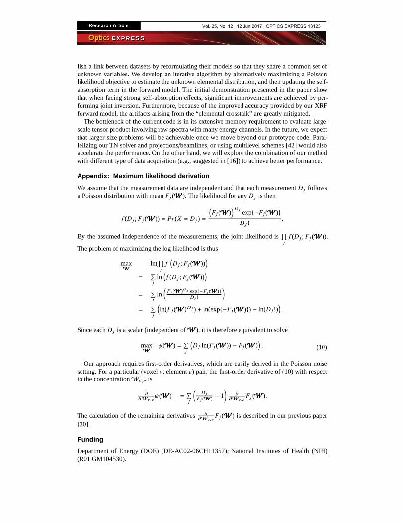
Appendix: Maximum likelihood derivation

We assume that the measurement data are independent and that each measurementD j followsa Poisson distribution with meanFj (WWW). The likelihood for anyD j is then

f (D j ; Fj (WWW)) = Pr(X = D j ) =

(

Fj (WWW))D j

exp−Fj (WWW)D j !

.

By the assumed independence of the measurements, the joint likelihood is∏

jf (D j ; Fj (WWW)).

The problem of maximizing the log likelihood is thus

maxWWW

ln(∏

j

f(

D j ; Fj (WWW)))

=∑

j

ln(

f (D j ; Fj (WWW)))

=∑

j

ln(

Fj (WWW)Dj exp−Fj (WWW)D j !

)

=∑

j

(

ln(Fj (WWW)D j ) + ln(exp−Fj (WWW)) − ln(D j !))

.

Since eachD j is a scalar (independent ofWWW), it is therefore equivalent to solve

maxWWW

ψ(WWW) =∑

j

(

D j ln(Fj (WWW)) − Fj (WWW))

. (10)

Our approach requires first-order derivatives, which are easily derived in the Poisson noisesetting. For a particular (voxelv, elemente) pair, the first-order derivative of (10) with respectto the concentrationWv ,e is

∂∂Wv ,e

ψ(WWW) =∑

j

(

D j

Fj (WWW) − 1)

∂∂Wv ,e

Fj (WWW).

The calculation of the remaining derivatives∂∂Wv ,e

Fj (WWW) is described in our previous paper[30].

Funding

Department of Energy (DOE) (DE-AC02-06CH11357); National Institutes of Health (NIH)(R01 GM104530).

Vol. 25, No. 12 | 12 Jun 2017 | OPTICS EXPRESS 13123

Acknowledgments

This material is based upon work supported by the U.S. Department of Energy, Office of Science,Offices of Advanced Scientific Computing Research and Basic Energy Sciences under ContractNo. DE-AC02-06CH11357. The work of YPH and CJ was supported in part by the NationalInstitutes of Health under grant R01 GM104530. The authors are grateful to Doga Gursoy andStefan Vogt for their help with and support of the TomoPy and MAPS codes.

Vol. 25, No. 12 | 12 Jun 2017 | OPTICS EXPRESS 13124