Joint & Progressive Learning fromHigh-Dimensional Data for Multi-Label

Classification

Danfeng Hong1,2[0000−0002−3212−9584], Naoto Yokoya3[0000−0002−7321−4590], JianXu1[0000−0003−2348−125X], and Xiaoxiang Zhu1,2[0000−0001−5530−3613]

1 Remote Sensing Technology Institute (IMF), German Aerospace Center (DLR),Wessling, Germany

{danfeng.hong,jian.xu,xiao.zhu}@dlr.de2 Signal Processing in Earth Observation (SiPEO), Technical University of Munich,

Munich, Germany3 RIKEN Center for Advanced Intelligence Project, Tokyo, Japan

{naoto.yokoya}@riken.jp

Abstract. Despite the fact that nonlinear subspace learning techniques(e.g. manifold learning) have successfully applied to data representation,there is still room for improvement in explainability (explicit mapping),generalization (out-of-samples), and cost-effectiveness (linearization). Tothis end, a novel linearized subspace learning technique is developed in ajoint and progressive way, called joint and progressive learning strategy(J-Play), with its application to multi-label classification. The J-Playlearns high-level and semantically meaningful feature representation fromhigh-dimensional data by 1) jointly performing multiple subspace learn-ing and classification to find a latent subspace where samples are ex-pected to be better classified; 2) progressively learning multi-coupledprojections to linearly approach the optimal mapping bridging the orig-inal space with the most discriminative subspace; 3) locally embeddingmanifold structure in each learnable latent subspace. Extensive experi-ments are performed to demonstrate the superiority and effectiveness ofthe proposed method in comparison with previous state-of-the-art meth-ods.

Keywords: Alternating direction method of multipliers ·High-dimensionaldata · Manifold regularization · Multi-label classification · Joint learning· Progressive learning

1 Introduction

High-dimensional data are often characterized by very rich and diverse informa-tion, which enables us to classify or recognize the targets more effectively andanalyze data attributes more easily, but inevitably introduces some drawback-s (e.g. information redundancy, complex noise effects, high storage-consuming,etc.) due to the curve of dimensionality. A general way to address this problem

2 D. Hong et al.

Original data space Label space

Subspace learning, e.g., PCA, LPP, LDA Classification

SubspaceOptimal subspace

Separately performing subspace learning and classification

Original data space Subspace Label space

Jointly conducting subspace learning and classification

Property-labeled projection PSubspace projection θ

Jointly and progressively learning with local manifold preserving

Label spaceOriginal data spaceLatent subspaces 1,...,

ll mθ

P

Local topological structure

Low HighFeature discriminative ability

Optimal classification

Enough to be represented by only single projection

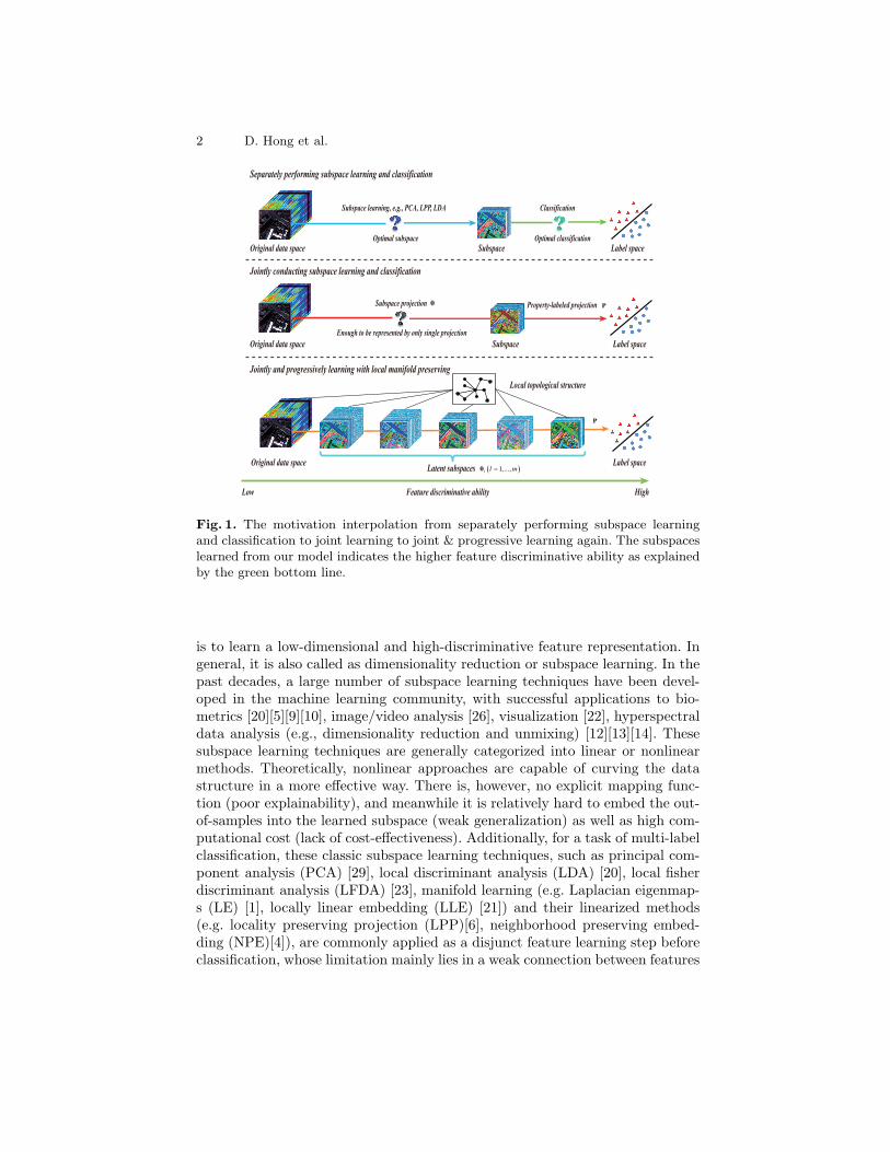
Fig. 1. The motivation interpolation from separately performing subspace learningand classification to joint learning to joint & progressive learning again. The subspaceslearned from our model indicates the higher feature discriminative ability as explainedby the green bottom line.

is to learn a low-dimensional and high-discriminative feature representation. Ingeneral, it is also called as dimensionality reduction or subspace learning. In thepast decades, a large number of subspace learning techniques have been devel-oped in the machine learning community, with successful applications to bio-metrics [20][5][9][10], image/video analysis [26], visualization [22], hyperspectraldata analysis (e.g., dimensionality reduction and unmixing) [12][13][14]. Thesesubspace learning techniques are generally categorized into linear or nonlinearmethods. Theoretically, nonlinear approaches are capable of curving the datastructure in a more effective way. There is, however, no explicit mapping func-tion (poor explainability), and meanwhile it is relatively hard to embed the out-of-samples into the learned subspace (weak generalization) as well as high com-putational cost (lack of cost-effectiveness). Additionally, for a task of multi-labelclassification, these classic subspace learning techniques, such as principal com-ponent analysis (PCA) [29], local discriminant analysis (LDA) [20], local fisherdiscriminant analysis (LFDA) [23], manifold learning (e.g. Laplacian eigenmap-s (LE) [1], locally linear embedding (LLE) [21]) and their linearized methods(e.g. locality preserving projection (LPP)[6], neighborhood preserving embed-ding (NPE)[4]), are commonly applied as a disjunct feature learning step beforeclassification, whose limitation mainly lies in a weak connection between features

Joint & Progressive Learning 3

by subspace learning and label space (see the top panel of Fig. 1). It is unknownwhich learned features (or subspace) can improve the classification.

Recently, a feasible solution to the above problems can be generalized as ajoint learning framework [17] that simultaneously considers linearized subspacelearning and classification, as illustrated in the middle panel of Fig. 1. Followingit, more advanced methods have been proposed and applied in various fields,including supervised dimensionality reduction (e.g. least-squares dimensionalityreduction (LSDR) [24] and its variants: least-squares quadratic mutual informa-tion derivative (LSQMID) [25]), multi-modal data matching and retrieval [28,27], and heterogeneous features learning for activity recognition [15, 16]. In thesework, the learned features (or subspace) and label information are effectively con-nected by regression techniques (e.g. linear regression) to adaptively estimate alatent and discriminative subspace. Despite this, they still fail to find an optimalsubspace, as single linear projection is hardly enough to represent the complextransformation from the original data space to the potential optimal subspace.

Motivated by the aforementioned studies, we propose a novel joint and progre-ssive learning strategy (J-Play) to linearly find an optimal subspace for generalmulti-label classification, illustrated in the bottom panel of Fig. 1. We practical-ly extend the existing joint learning framework by learning a series of subspacesinstead of single subspace, aiming at progressively converting the original da-ta space to a potentially optimal subspace through multi-coupled intermediatetransformations [18]. Theoretically, by increasing the number of subspaces, cou-pled subspace variations are gradually narrowed down to a very small range thatcan be represented effectively via a linear transformation. This renders us to finda good solution easier, especially when the model is complex and non-convex.We also contribute to structure learning in each latent subspace by locally em-bedding manifold structure.

The main highlights of our work can be summarized as follows:

– A linearized progressive learning strategy is proposed to describe the varia-tions from the original data space to potentially optimal subspace, tendingto find a better solution. A joint learning framework that simultaneouslyestimates subspace projections (connect the original space and the laten-t subspaces) and a property-labeled projection (connect the learned latentsubspaces and label space) is considered to find a discriminative subspacewhere samples are expected to be better classified.

– Structure learning with local manifold regularization is performed in eachlatent subspace.

– Based on the above techniques, a novel joint and progressive learning strat-egy (J-Play) is developed for multi-label classification.

– An iterative optimization algorithm based on the alternating direction methodof multipliers (ADMM) is designed to solve the proposed model.

4 D. Hong et al.

2 Joint & Progressive Learning Strategy (J-Play)

2.1 Notations

Let X = [x1, ...,xk, ...,xN ] ∈ Rd0×N be a data matrix with d0 dimensions and

N samples, and the matrix of corresponding class labels be Y ∈ {0, 1}L×N . Thekth column of Y is yk = [yk1, ...,ykt, ...,ykL]

T ∈ RL×1 whose each element can

be defined as follows:

ykt =

{

1, if yk belongs to the t-th class;

0, otherwise.(1)

In our task, we aim to learn a set of coupled projections {Θl}ml=1 ∈ R

dl×dl−1 anda property-labeled projection P ∈ R

L×dm , where m stands for the number ofsubspace projections and {dl}

ml=1 are defined as the dimensions of those latent

subspaces respectively, while d0 is specified as the dimension of X.

2.2 Basic Framework of J-Play from the View of Subspace Learning

Subspace learning is to find a low-dimensional space where we expect to maxi-mize certain properties of the original data, e.g. variance (PCA), discriminativeability (LDA), and graph structure (manifold learning). Yan et al. [30] summa-rized these subspace learning methods in a general graph embedding framework.

Given an undirected similarity graph G = {X,W} with the vertices X ∈{x1, ...,xN} and the adjacency matrix W ∈ R

N×N , we can intuitively measurethe similarities among the data. By preserving the similarities relationship, thehigh-dimensional data can be well embedded into the low-dimensional space,which can be formulated by denoting the low-dimensional data representationas Z ∈ R

d×N (d≪ d0) in the following

minZ

tr(ZLZT), s.t. ZDZT = I, (2)

where Dii =∑

j Wij is a diagonal matrix, L is a Laplacian matrix defined byL = D −W [3], and I is the identity matrix. In our case, we aim at learningmulti-coupled linear projections to find optimal mapping, therefore a linearizedsubspace learning problem can be reformulated on the basis of Eq. (2) by sub-stituting ΘX for Z

minΘ

tr(ΘXLXTΘT), s.t. ΘXDXTΘT = I, (3)

which can be solved by generalized eigenvalue decomposition.Different from the previously mentioned subspace learning methods, a re-

gression-based joint learning model [17] can explicitly bridge the learned latentsubspace and labels, which can be formulated in a general form:

minP,Θ

1

2E(P,Θ) +

β

2Φ(Θ) +

γ

2Ψ(P), (4)

Joint & Progressive Learning 5

1θ

2θ

3θ

4θ

5θ

5

Tθ

4

Tθ

3

Tθ

2

Tθ

1

Tθ

P

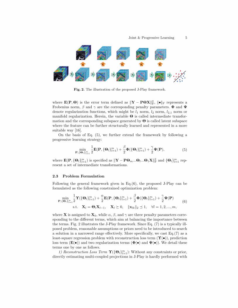
Fig. 2. The illustration of the proposed J-Play framework.

where E(P,Θ) is the error term defined as ‖Y − PΘX‖2F, ‖•‖F represents aFrobenius norm, β and γ are the corresponding penalty parameters. Φ and Ψ

denote regularization functions, which might be l1 norm, l2 norm, l2,1 norm ormanifold regularization. Herein, the variable Θ is called intermediate transfor-mation and the corresponding subspace generated by Θ is called latent subspacewhere the feature can be further structurally learned and represented in a moresuitable way [16].

On the basis of Eq. (5), we further extend the framework by following aprogressive learning strategy:

minP,{Θl}ml=1

1

2E(P, {Θl}

ml=1) +

β

2Φ({Θl}

ml=1) +

γ

2Ψ(P), (5)

where E(P, {Θl}ml=1) is specified as ‖Y−PΘm...Θl...Θ1X‖

2F and {Θl}

ml=1 rep-

resent a set of intermediate transformations.

2.3 Problem Formulation

Following the general framework given in Eq.(6), the proposed J-Play can beformulated as the following constrained optimization problem:

minP,{Θl}ml=1

1

2Υ({Θl}

ml=1) +

α

2E(P, {Θl}

ml=1) +

β

2Φ({Θl}

ml=1) +

γ

2Ψ(P)

s.t. Xl = ΘlXl−1, Xl � 0, ‖xlk‖2 � 1, ∀l = 1, 2, ...,m,

(6)

where X is assigned to X0, while α, β, and γ are three penalty parameters corre-sponding to the different terms, which aim at balancing the importance betweenthe terms. Fig. 2 illustrates the J-Play framework. Since Eq. (7) is a typically ill-posed problem, reasonable assumptions or priors need to be introduced to searcha solution in a narrowed range effectively. More specifically, we cast Eq.(7) as aleast-square regression problem with reconstruction loss term (Υ(•)), predictionloss term (E(•)) and two regularization terms (Φ(•) and Ψ(•)). We detail theseterms one by one as follows.

1) Reconstruction Loss Term Υ({Θl}ml=1): Without any constraints or prior,

directly estimating multi-coupled projections in J-Play is hardly performed with

6 D. Hong et al.

the increase of the number of estimated projections. This can be reasonablyexplained by gradient missing between the two neighboring variables estimatedin the process of optimization. That is, the variations between these neighboringprojections are made to be tiny and even zero. In particular, when the numberof projections increases to a certain extent, most of learned projections tend tobe zero and become meaningless. To this end, we adopt a kind of autoencoder-like scheme to make the learned subspace projected back to the original spaceas much as possible. The benefits of the scheme are, on one hand, to preventthe data over-fitting to some extent, especially avoiding overmuch noises frombeing considered; on the other hand, to establish an effective link between theoriginal space and the subspace, making the learned subspace more meaningful.Therefore, the resulting expression is

Υ({Θl}ml=1) =

∑m

l=1‖Xl−1 −ΘT

l ΘlXl−1‖2F. (7)

In our case, to fully utilize the advantages of this term, we consider it in eachlatent subspace as shown in Eq.(8).

2) Predication Loss Term E(P, {Θl}ml=1): This term is to minimize the empir-

ical risk between the original data and the corresponding labels through multi-coupled projections in a progressive way, which can be formulated as

E(P, {Θl}ml=1) = ‖Y −PΘm...Θl...Θ1X‖

2F. (8)

3) Local Manifold Regularization Φ({Θl}ml=1): As introduced in [27], a man-

ifold structure is an important prior for subspace learning. Superior to vector-based feature learning, such as artificial neural network (ANN), a manifold struc-ture can effectively capture the intrinsic structure between samples. To facilitatestructure learning in J-Play, we perform the local manifold regularization to eachlatent subspace. Specifically, this term can be expressed by

Φ({Θl}ml=1) =

∑m

l=1tr(ΘlXl−1LX

Tl−1Θ

Tl ). (9)

4) Regression Coefficient Regularization Ψ(P): The regularization term can pro-mote us to derive a more reasonable solution with a reliable generalization toour model, which can be written as

Ψ(P) = ‖P‖2F. (10)

Moreover, the non-negativity constraint with respect to each learned dimension-reduced feature (e.g. {Xl}

ml=1 � 0) is considered since we aim to obtain a mean-

ingful low-dimensional feature representation similar to original image data ac-quired in a non-negative unit. In addition to the non-negativity constraint, wealso impose a norm constraint 4 for sample-based of each subspace: ‖xlk‖2 �1, ∀k = 1, ..., N and l = 1, ...,m.

4 Regarding this constraint,please refer to [19] for more details.

Joint & Progressive Learning 7

Algorithm 1: Joint & Progressive Learning Strategy (J-Play)Input: Y,X,L, and parameters α, β, γ and maxIter.Output: {Θl}

ml=1.

1 Initialization Step:

2 Greedily initialize Θl corresponding to each latent subspace:3 for l = 1 : m do

4 Θ0l ← LPP (Xl−1)

5 Θl ← AutoRULe(Xl−1,Θ0l ,L)

6 Xl ← ΘlXl−1

7 end

8 Fine-tuning Step:

9 t = 0, ζ = 1e− 4;10 while not converged or t > maxIter do

11 Fix other variables to update P by solving a subproblem of P;12 for i = 1 : m do

13 Fix other variables to update Θt+1

lby solving a subproblem of Θl;

14 end

15 Compute the objective function value Objt+1 and check the convergence condition: if

|Objt+1−Objt

Objt| < ζ then

16 Stop iteration;17 else

18 t← t + 1;19 end

20 end

2.4 Model Optimization

Considering the complexity and the non-convexity of our model, we pretrain ourmodel to have an initial approximation of subspace projections {Θl}

ml=1 as this

can greatly reduce the model’s training time and also help finding an optimalsolution easier. This is a common tactic that has been successfully employed indeep autoencoders [8]. Inspired by this trick, we propose a pre-training modelwith respect to Θl, ∀l = 1, ...,m by simplifying Eq.(7) as

minΘl

1

2Υ(Θl) +

η

2Φ(Θl) s.t. Xl � 0, ‖xlk‖2 � 1, (11)

which is named as auto-reconstructing unsupervised learning (AutoRULe).Given the outputs of AutoRULe, the problem of Eq. (7) can be more effec-tively solved by an alternatively minimizing strategy that separately solves twosubproblems with respect to {Θl}

ml=1 and P. Therefore, the global algorithm of

J-Play can be summarized in Algorithm 1,where AutoRULe is initialized byLPP.

The pre-training method (AutoRULe) can be effectively solved via the ADMM-based framework. Following this, we consider an equivalent form of Eq. (12) byintroducing multiple auxiliary variables H, G, Q and S to replace Xl, Θl, X

+l

and X∼l , respectively, where ()+ denotes an operator that converts each com-ponent of the matrix to its absolute value and ()∼ is a proximal operator for

8 D. Hong et al.

solving the constraint of ‖xlk‖2 � 1 [7], written as follows

minΘl,H,G,Q,S

1

2Υ(G,H) +

η

2Φ(Θl) =

1

2‖Xl−1 −GTH‖2F +

η

2tr(XlLX

Tl )

s.t. Q � 0, ‖sk‖2 � 1, Xl = ΘlXl−1,

Xl = H, Θl = G, Xl = Q, Xl = S.

(12)

The augmented Lagrangian version of Eq. (13) is

L µ

(

Θl,H,G,Q,S, {Λn}4n=1

)

=1

2‖Xl−1 −GTH‖2F +

η

2tr(ΘlXl−1LX

Tl−1Θ

Tl ) +ΛT

1 (H−ΘlXl−1)

+ΛT2 (G−Θl) +ΛT

3 (Q−ΘlXl−1) +ΛT4 (S−ΘlXl−1) +

µ

2‖H−ΘlXl−1‖

2F

+µ

2‖G−Θl‖

2F +

µ

2‖Q−ΘlXl−1‖

2F +

µ

2‖S−ΘlXl−1‖

2F + l+R(Q) + l∼R(S),

(13)where {Λn}

4n=1 are Lagrange multipliers and µ is the penalty parameter. The two

terms l+R(•) and l∼R(•) represent two kinds of projection operators, respectively.That is, l+R(•) is defined as

max(•) =

{

• , • ≻ 0

0 , • � 0,(14)

while l∼R(•k) is a vector-based operator defined by

proxf (•k) =

{

•k‖•k‖2

, ‖•k‖2 ≻ 1

•k , ‖•k‖2 � 1,(15)

where •k is the kth column of matrix •. Algorithm 2 details the procedures ofAutoRULe.

The two subproblems in Algorithm 1 can be optimized alternatively asfollows:

Optimization with respect to P: This is a typical least square regression prob-lem, which can be written as

minP

α

2E(P) +

γ

2Ψ(P) =

α

2‖Y −PΘm...Θl...Θ1X‖

2F +

γ

2‖P‖2F, (16)

which has a closed-form solution

P← (αYVT)(αVVT + γI)−1, (17)

where V = Θm...Θl...Θ1, ∀l = 1, ...,m.

Optimization with respect to {Θl}ml=1: The variables {Θl}

ml=1 can be individ-

ually optimized, and hence the optimization problem of each Θl can be generally

Joint & Progressive Learning 9

Algorithm 2: Auto-reconstructing unsupervised learning (AutoRULe)

Input: Xl−1,Θ0l ,L, and parameters η and maxIter.

Output: Θl.1 Initialization: H0 = Θ0

l Xl−1,G0 = 0,Q0 = P0 = 0,Λ0

2 = 0,Λ01 = Λ0

3 = Λ04 = 0, µ0 =

1e− 3, µmax = 1e6, ρ = 2, ε = 1e− 6, t = 0.2 while not converged or t > maxIter do

3 Fix Ht,Gt,Qt,Pt to update Θt+1

lby

Θl =(µHXTl−1 + Λ1X

Tl−1 + µG + Λ2 + µQX

Tl−1 + Λ3X

Tl−1

+ µPXTl−1 + Λ4X

Tl−1)(η(Xl−1LX

Tl−1) + 3µ(Xl−1X

Tl−1) + µI)

−1.

4 Fix Θt+1

l,Gt,Qt,Pt to update Ht+1 by

H = (GGT

+ µI)−1

(GXl−1 + µΘlXl−1 −Λ1).

5 Fix Ht+1,Θt+1

l,Qt,Pt to update Gt+1 by

G = (HHT

+ µI)−1

(HXi + µΘl −Λ2).

6 Fix Ht+1,Gt+1,Θt+1

l,Pt to update Qt+1 by

Q = max(ΘlXl−1 −Λ3/µ, 0).

7 Fix Ht+1,Gt+1,Θt+1

l,Qt+1 to update Pt+1 by

P = proxf (ΘlXl−1 −Λ4/µ).

8 Update Lagrange multipliers by

Λt+1

1 = Λt1 + µ

t(H

t+1−Θ

t+1

i Xl−1),Λt+1

2 = Λt2 + µ

t(G

t+1−Θ

t+1

i ),

Λt+1

3 = Λt3 + µ

t(Q

t+1−Θ

t+1

i Xl−1),Λt+1

4 = Λt4 + µ

t(P

t+1−Θ

t+1

i Xl−1).

9 Update penalty parameter by

µt+1

= min(ρµt, µmax).

10 Check the convergence conditions: if ‖Ht+1 −Θt+1

lXl−1‖F < ε and

‖Gt+1 −Θt+1

l‖F < ε and ‖Qt+1 −Θ

t+1

lXl−1‖F < ε and

‖Pt+1 −Θt+1

lXl−1‖F < ε then

11 Stop iteration;12 else

13 t← t + 1;14 end

15 end

formulated by

minΘl

1

2Υ(Θl) +

α

2E(Θl) +

β

2Φ(Θl) =

1

2‖Xl−1 −ΘT

l ΘlXl−1‖2F

+α

2‖Y −PΘm...Θl...Θ1X‖

2F +

β

2tr(ΘlXl−1LX

Tl−1Θ

Tl )

s.t. Xl = ΘlXl−1, Xl � 0, ‖xlk‖2 � 1,

(18)

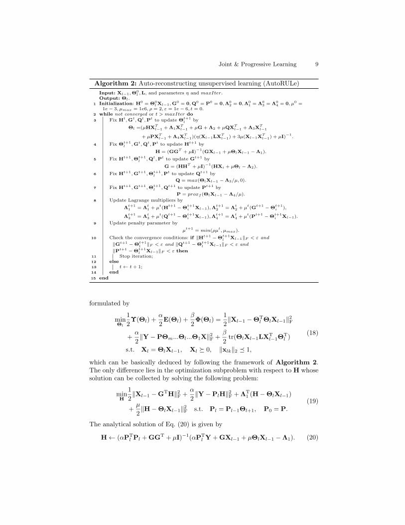
which can be basically deduced by following the framework of Algorithm 2.The only difference lies in the optimization subproblem with respect to H whosesolution can be collected by solving the following problem:

minH

1

2‖Xl−1 −GTH‖2F +

α

2‖Y −PlH‖

2F +ΛT

1 (H−ΘlXl−1)

+µ

2‖H−ΘlXl−1‖

2F s.t. Pl = Pl−1Θl+1, P0 = P.

(19)

The analytical solution of Eq. (20) is given by

H← (αPTl Pl +GGT + µI)−1(αPT

l Y +GXl−1 + µΘlXl−1 −Λ1). (20)

10 D. Hong et al.

Finally, we repeat these optimization procedures until a stopping criterion issatisfied. Please refer to Algorithm 1 and Algorithm 2 for more explicit steps.

3 Experiments

In this section, we conduct the classification to quantitatively evaluate the per-formance of the proposed method (J-Play) using three popular and advancedclassifiers, namely the nearest neighbor (NN) based on the Euclidean distance,kernel support vector machines (KSVM) and canonical correlation forest (CCF),in comparison with previous state-of-the-art methods. Overall accuracy (OA) isgiven to quantify the classification performance.

3.1 Data Description

The experiments are performed on two different types of datasets: hyperspectraldatasets and face datasets, as both of them easily suffer from the informationredundancy and need to improve the representative ability of features. We haveused the following two hyperspectral datasets and two face datasets:

1) Indian Pines AVIRIS Image: The first hyperspectral cube was acquiredby the AVIRIS sensor with the size of 145 × 145 × 220, which consists of 16class of vegetation. More specific classes and the arrangement of training andtest samples can be found in [11]. The first image of Fig. 3 shows a false colorimage of Indian Pines data.

2) University of Houston Image: The second hyperspectral cube was providedfor the 2013 IEEE GRSS data fusion contest acquired by ITRES-CASI sensorwith size of 349×1905×144. The information regarding classes and correspondingtrain and test samples can be found in [13]. A false color image of the study sceneis shown in the first image of Fig. 4.

3) Extended Yale-B Dataset: We only choose a subset of the mentioneddataset with the frontal pose and the different illuminations of 38 subjects (2414images in total), which can widely used in evaluating the performance of sub-space learning [32][2]. These images were aligned and cropped to the size of32 × 32, that is, 1024-dimensional vector-based representation. Each individualhas 64 near frontal images under different illuminations.

4) AR Dataset: Similar to [31], we choose a subset of AR under the conditionsof illumination and expressions, which comprises of 100 subjects. Each personhas 14 images with seven ones from Session 1 as training set and others fromSession 2 as testing samples. The images are resized to 60× 43.

3.2 Experimental Steup

As the fixed training and testing samples are given for the hyperspectral datasets,subspace learning techniques can directly be performed on training set to learnan optimal subspace where the testing set can be simply classified by NN, KSVM,and CCF. For the face datasets, since there is no standard training and testing

Joint & Progressive Learning 11

CornNotill CornMintill Corn GrassPature GrassTrees HayWindrow SoybeanNotil SoybeanMintill SoybeanClean Wheat Woods BuilGraTrDri StoSteTower Alfalfa GrasPastMow Oats

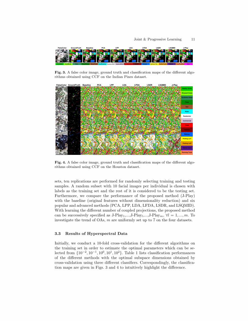
FalseColor GroundTruth Baseline PCA LPP LDA LFDA LSDR LSQMID J-Play

Fig. 3. A false color image, ground truth and classification maps of the different algo-rithms obtained using CCF on the Indian Pines dataset.

Healthy Grass

Stressed Grass

Synthetic Grass

Trees

Soil

Water

Residential

Commercial

Road

Highway

Railway

Parking Lot1

Parking Lot2

Tennis Court

Running Track

FalseColor GroundTruth Baseline PCA LPP LDA LFDA LSDR LSQMID J-Play

Fig. 4. A false color image, ground truth and classification maps of the different algo-rithms obtained using CCF on the Houston dataset.

sets, ten replications are performed for randomly selecting training and testingsamples. A random subset with 10 facial images per individual is chosen withlabels as the training set and the rest of it is considered to be the testing set.Furthermore, we compare the performance of the proposed method (J-Play)with the baseline (original features without dimensionality reduction) and sixpopular and advanced methods (PCA, LPP, LDA, LFDA, LSDR, and LSQMID).With learning the different number of coupled projections, the proposed methodcan be successively specified as J-Play1,...,J-Playl,...,J-Playm, ∀l = 1, ...,m. Toinvestigate the trend of OAs, m are uniformly set up to 7 on the four datasets.

3.3 Results of Hyperspectral Data

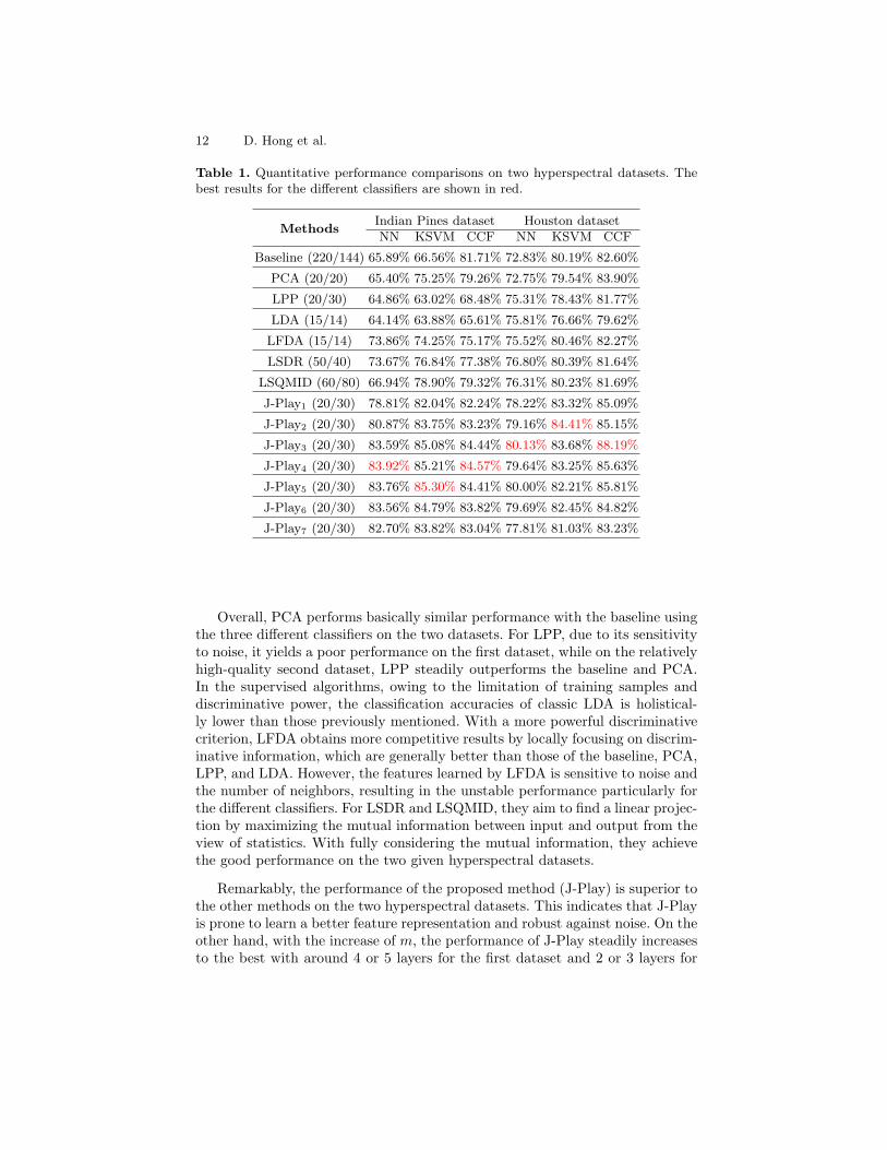
Initially, we conduct a 10-fold cross-validation for the different algorithms onthe training set in order to estimate the optimal parameters which can be se-lected from {10−2, 10−1, 100, 101, 102}. Table 1 lists classification performancesof the different methods with the optimal subspace dimensions obtained bycross-validation using three different classifiers. Correspondingly, the classifica-tion maps are given in Figs. 3 and 4 to intuitively highlight the difference.

12 D. Hong et al.

Table 1. Quantitative performance comparisons on two hyperspectral datasets. Thebest results for the different classifiers are shown in red.

MethodsIndian Pines dataset Houston datasetNN KSVM CCF NN KSVM CCF

Baseline (220/144) 65.89% 66.56% 81.71% 72.83% 80.19% 82.60%

PCA (20/20) 65.40% 75.25% 79.26% 72.75% 79.54% 83.90%

LPP (20/30) 64.86% 63.02% 68.48% 75.31% 78.43% 81.77%

LDA (15/14) 64.14% 63.88% 65.61% 75.81% 76.66% 79.62%

LFDA (15/14) 73.86% 74.25% 75.17% 75.52% 80.46% 82.27%

LSDR (50/40) 73.67% 76.84% 77.38% 76.80% 80.39% 81.64%

LSQMID (60/80) 66.94% 78.90% 79.32% 76.31% 80.23% 81.69%

J-Play1 (20/30) 78.81% 82.04% 82.24% 78.22% 83.32% 85.09%

J-Play2 (20/30) 80.87% 83.75% 83.23% 79.16% 84.41% 85.15%

J-Play3 (20/30) 83.59% 85.08% 84.44% 80.13% 83.68% 88.19%

J-Play4 (20/30) 83.92% 85.21% 84.57% 79.64% 83.25% 85.63%

J-Play5 (20/30) 83.76% 85.30% 84.41% 80.00% 82.21% 85.81%

J-Play6 (20/30) 83.56% 84.79% 83.82% 79.69% 82.45% 84.82%

J-Play7 (20/30) 82.70% 83.82% 83.04% 77.81% 81.03% 83.23%

Overall, PCA performs basically similar performance with the baseline usingthe three different classifiers on the two datasets. For LPP, due to its sensitivityto noise, it yields a poor performance on the first dataset, while on the relativelyhigh-quality second dataset, LPP steadily outperforms the baseline and PCA.In the supervised algorithms, owing to the limitation of training samples anddiscriminative power, the classification accuracies of classic LDA is holistical-ly lower than those previously mentioned. With a more powerful discriminativecriterion, LFDA obtains more competitive results by locally focusing on discrim-inative information, which are generally better than those of the baseline, PCA,LPP, and LDA. However, the features learned by LFDA is sensitive to noise andthe number of neighbors, resulting in the unstable performance particularly forthe different classifiers. For LSDR and LSQMID, they aim to find a linear projec-tion by maximizing the mutual information between input and output from theview of statistics. With fully considering the mutual information, they achievethe good performance on the two given hyperspectral datasets.

Remarkably, the performance of the proposed method (J-Play) is superior tothe other methods on the two hyperspectral datasets. This indicates that J-Playis prone to learn a better feature representation and robust against noise. On theother hand, with the increase of m, the performance of J-Play steadily increasesto the best with around 4 or 5 layers for the first dataset and 2 or 3 layers for

Joint & Progressive Learning 13

(a) Extended Yale-B dataset (b) AR dataset

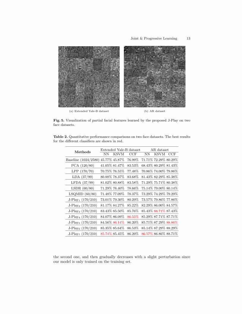
Fig. 5. Visualization of partial facial features learned by the proposed J-Play on twoface datasets.

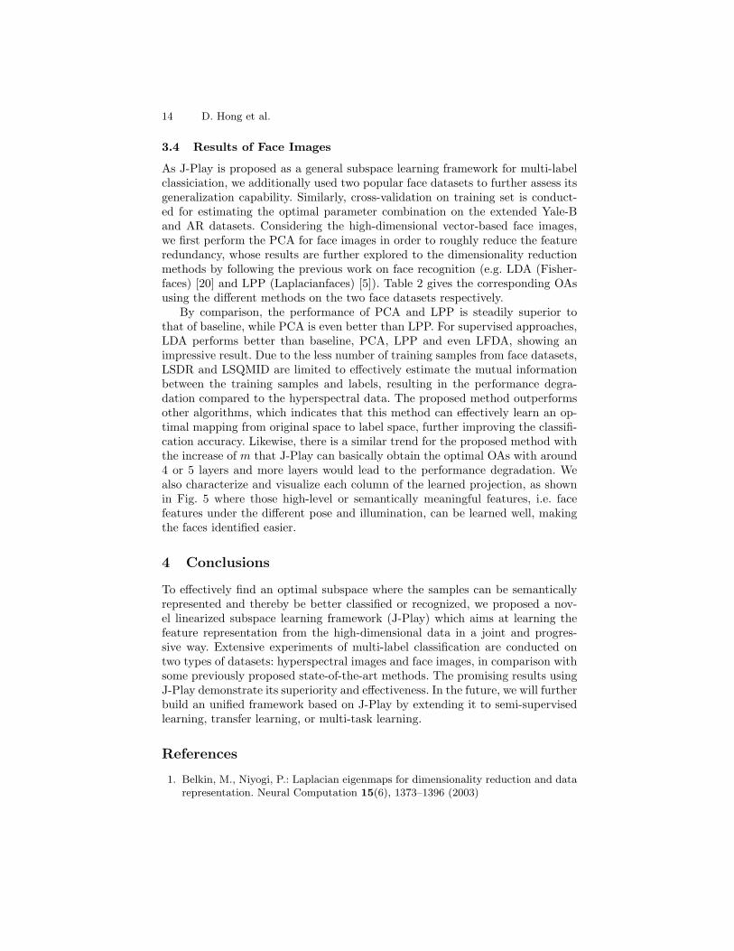
Table 2. Quantitative performance comparisons on two face datasets. The best resultsfor the different classifiers are shown in red.

MethodsExtended Yale-B dataset AR datasetNN KSVM CCF NN KSVM CCF

Baseline (1024/2580) 45.77% 45.87% 76.99% 71.71% 72.29% 80.29%

PCA (120/80) 41.05% 81.47% 83.53% 68.43% 80.29% 81.43%

LPP (170/70) 70.75% 76.55% 77.48% 70.86% 74.00% 79.86%

LDA (37/99) 80.88% 78.37% 83.68% 81.43% 82.29% 85.38%

LFDA (37/99) 81.02% 80.88% 83.58% 71.29% 75.71% 80.38%

LSDR (60/80) 71.29% 76.40% 78.66% 75.14% 79.00% 80.14%

LSQMID (60/80) 71.48% 77.09% 78.37% 73.29% 74.29% 79.29%

J-Play1 (170/210) 73.01% 79.30% 80.29% 73.57% 79.86% 77.86%

J-Play2 (170/210) 81.17% 84.27% 85.22% 82.29% 86.00% 84.57%

J-Play3 (170/210) 83.43% 85.50% 85.76% 85.43% 88.71% 87.43%

J-Play4 (170/210) 84.07% 86.09% 86.55% 85.29% 87.71% 87.71%

J-Play5 (170/210) 84.56% 86.14% 86.20% 85.71% 87.29% 88.86%

J-Play6 (170/210) 85.35% 85.64% 86.53% 85.14% 87.29% 88.29%

J-Play7 (170/210) 85.74% 85.45% 86.20% 86.57% 86.86% 88.71%

the second one, and then gradually decreases with a slight perturbation sinceour model is only trained on the training set.

14 D. Hong et al.

3.4 Results of Face Images

As J-Play is proposed as a general subspace learning framework for multi-labelclassiciation, we additionally used two popular face datasets to further assess itsgeneralization capability. Similarly, cross-validation on training set is conduct-ed for estimating the optimal parameter combination on the extended Yale-Band AR datasets. Considering the high-dimensional vector-based face images,we first perform the PCA for face images in order to roughly reduce the featureredundancy, whose results are further explored to the dimensionality reductionmethods by following the previous work on face recognition (e.g. LDA (Fisher-faces) [20] and LPP (Laplacianfaces) [5]). Table 2 gives the corresponding OAsusing the different methods on the two face datasets respectively.

By comparison, the performance of PCA and LPP is steadily superior tothat of baseline, while PCA is even better than LPP. For supervised approaches,LDA performs better than baseline, PCA, LPP and even LFDA, showing animpressive result. Due to the less number of training samples from face datasets,LSDR and LSQMID are limited to effectively estimate the mutual informationbetween the training samples and labels, resulting in the performance degra-dation compared to the hyperspectral data. The proposed method outperformsother algorithms, which indicates that this method can effectively learn an op-timal mapping from original space to label space, further improving the classifi-cation accuracy. Likewise, there is a similar trend for the proposed method withthe increase of m that J-Play can basically obtain the optimal OAs with around4 or 5 layers and more layers would lead to the performance degradation. Wealso characterize and visualize each column of the learned projection, as shownin Fig. 5 where those high-level or semantically meaningful features, i.e. facefeatures under the different pose and illumination, can be learned well, makingthe faces identified easier.

4 Conclusions

To effectively find an optimal subspace where the samples can be semanticallyrepresented and thereby be better classified or recognized, we proposed a nov-el linearized subspace learning framework (J-Play) which aims at learning thefeature representation from the high-dimensional data in a joint and progres-sive way. Extensive experiments of multi-label classification are conducted ontwo types of datasets: hyperspectral images and face images, in comparison withsome previously proposed state-of-the-art methods. The promising results usingJ-Play demonstrate its superiority and effectiveness. In the future, we will furtherbuild an unified framework based on J-Play by extending it to semi-supervisedlearning, transfer learning, or multi-task learning.

References

1. Belkin, M., Niyogi, P.: Laplacian eigenmaps for dimensionality reduction and datarepresentation. Neural Computation 15(6), 1373–1396 (2003)

Joint & Progressive Learning 15

2. Cai, D., He, X., Han, J.: Spectral regression: A unified approach for sparse subspacelearning. In: International Conference on Data Mining (ICDM). pp. 73–82 (2007)

3. Chung, F.R.K.: Spectral graph theory. American Mathematical Society (1997)

4. He, X., Cai, D., Yan, S., Zhang, H.J.: Neighborhood preserving embedding. In:International Conference on Computer Vision (ICCV). vol. 2, pp. 1208–1213 (2005)

5. He, X., Hu, S., Niyogi, P., Zhang, H.J.: Face recognition using laplacianfaces. IEEETransactions on Pattern Analysis and Machine Intelligence (TPAMI) 27(3), 328–340 (2005)

6. He, X., Niyogi, P.: Locality preserving projections. In: Advances in Neural Infor-mation Processing Systems (NIPS). pp. 153–160 (2004)

7. Heide, F., Heidrich, W., Wetzstein, G.: Fast and flexible convolutional sparse cod-ing. In: IEEE Conference on Computer Vision and Pattern Recognition (CVPR).pp. 5135–5143 (2015)

8. Hinton, G.E., Salakhutdinov, R.R.: Reducing the dimensionality of data with neu-ral networks. Science 313(5786), 504–507 (2006)

9. Hong, D., Liu, W., Su, J., Z.Pan, Wang, G.: A novel hierarchical approach formultispectral palmprint recognition. Neurocomputing 151, 511–521 (2015)

10. Hong, D., Liu, W., Wu, X., Pan, Z., Su, J.: Robust palmprint recognition basedon the fast variation vese–osher model. Neurocomputing 174, 999–1012 (2016)

11. Hong, D., Yokoya, N., Zhu, X.: The k-lle algorithm for nonlinear dimensionalityruduction of large-scale hyperspectral data. In: IEEE Workshop on HyperspectralImage and Signal Processing: Evolution in Remote Sensing (WHISPERS). pp. 1–5.IEEE (2016)

12. Hong, D., Yokoya, N., Zhu, X.: Local manifold learning with robust neighbors selec-tion for hyperspectral dimensionality reduction. In: IEEE International Conferenceon Geoscience and Remote Sensing Symposium (IGARSS). pp. 40–43. IEEE (2016)

13. Hong, D., Yokoya, N., Zhu, X.: Learning a robust local manifold representation forhyperspectral dimensionality reduction. IEEE Journal of Selected Topics in Ap-plied Earth Observations and Remote Sensing (JSTARS) 10(6), 2960–2975 (2017)

14. Hong, D., Yokoya, N., Chanussot, J., Zhu, X.X.: Learning a low-coherence dictio-nary to address spectral variability for hyperspectral unmixing. In: Image Process-ing (ICIP), 2017 IEEE International Conference on. pp. 235–239. IEEE (2017)

15. Hu, J., Zheng, W., Lai, J., Zhang, J.: Jointly learning heterogeneous features forrgb-d activity recognition. In: IEEE Conference on Computer Vision and PatternRecognition (CVPR). pp. 5344–5352 (2015)

16. Hu, J., Zheng, W., Lai, J., Zhang, J.: Jointly learning heterogeneous features forrgb-d activity recognition (2016)

17. Ji, S., Ye, J.: Linear dimensionality reduction for multi-label classification. In:International Joint Conference on Artifical Intelligence (IJCAI). vol. 9, pp. 1077–1082 (2009)

18. Kan, M., Shan, S., Chang, H., Chen, X.: Stacked progressive auto-encoders (spae)for face recognition across poses. In: IEEE Conference on Computer Vision andPattern Recognition (CVPR). pp. 1883–1890 (2014)

19. Lee, H., Battle, A., Raina, R., Ng, A.Y.: Efficient sparse coding algorithms. In:Advances in Neural Information Processing Systems (NIPS). pp. 801–808 (2007)

20. Martnez, A.M., Avinash, C.K.: Pca versus lda. IEEE Transactions on PatternAnalysis and Machine Intelligence (TPAMI) 23(2), 228–233 (2001)

21. Roweis, S.T., Lawrence, K.S.: Nonlinear dimensionality reduction by locally linearembedding. Science 290(5500), 2323–2326 (2000)

16 D. Hong et al.

22. Saul, S.L., Roweis, S.T.: Think globally, fit locally: unsupervised learning of lowdimensional manifolds. Journal of Machine Learning Research (JMLR) 4, 119–155(2003)

23. Sugiyama, M.: Dimensionality reduction of multimodal labeled data by local fisherdiscriminant analysis. Journal of Machine Learning Research (JMLR) 8, 1027–1061(2007)

24. Suzuki, T., Sugiyama, M.: Sufficient dimension reduction via squared-loss mutualinformation estimation. Neural Computation 25(3), 725–758 (2013)

25. Tangkaratt, V., Sasaki, H., Sugiyama, M.: Direct estimation of the derivative ofquadratic mutual information with application in supervised dimension reduction.Neural Computation 29(8), 2076–2122 (2017)

26. Tosato, D., Farenzena, M., Spera, M., Murino, V., Cristani, M.: Multi-class classi-fication on riemannian manifolds for video surveillance. In: Europe Conference onComputer Vision (ECCV). pp. 378–391 (2010)

27. Wang, K., He, R., Wang, L., Wang, W., Tan, T.: Joint feature selection and sub-space learning for cross-modal retrieval. IEEE Transactions on Pattern Analysisand Machine Intelligence (TPAMI) 38(10), 2010–2023 (2016)

28. Wang, K., He, R., Wang, W., Wang, L., Tan, T.: Learning coupled feature spaces forcross-modal matching. In: International Conference on Computer Vision (ICCV).pp. 2088–2095 (2013)

29. Wold, S., Esbensen, K., Geladi, P.: Principal component analysis. Chemometricsand Intelligent Laboratory Systems 2(1), 37–52 (1987)

30. Yan, S., Xu, D., Zhang, B., Zhang, H.J., Yang, Q., Lin, S.: Graph embedding andextensions: A general framework for dimensionality reduction. IEEE Transactionson Pattern Analysis and Machine Intelligence (TPAMI) 29(1), 40–51 (2007)

31. Yang, M., Zhang, L., Yang, J., Zhang, D.: Robust sparse coding for face recognition.In: IEEE Conference on Computer Vision and Pattern Recognition (CVPR). pp.625–632 (2011)

32. Zhang, L., Yang, M., Feng, X.: Sparse representation or collaborative represen-tation: which helps face recognition?. In: International Conference on ComputerVision (ICCV). pp. 471–478 (2011)