JOINT PROBABILITY ANALYSIS OF HURRICANE FLOOD

HAZARDS FOR MISSISSIPPI

Final Report

Prepared for

URS Group Tallahassee, FL

in support of the FEMA-HMTAP

flood study of the State of Mississippi

by

Gabriel R. Toro Risk Engineering, Inc.

4155 Darley Avenue, suite A Boulder, CO 80305

Revision 1 - June 23, 2008

ii

ABSTRACT

This report documents the development of a probabilistic model to represent the occurrence rate

and characteristics of future hurricanes capable of producing significant surge inundation along

the Mississippi coast, using available hurricane data and statistical tools that have been

developed for the offshore oil industry. The report also documents the generation of a suite of

synthetic storms, and associated recurrence rates, which provide an efficient representation of the

population of possible future hurricanes and their characteristics, for use as inputs to numerical

wind, wave, and surge models. These synthetic storms are generated by means of a JPM-OS

(Joint-Probability Method—Optimal Sampling) scheme, which is also described in the report.

iii

CONTENTS 1 Introduction .............................................................................................................................. 1

1.1 Project objectives ............................................................................................................ 1

1.2 Approach......................................................................................................................... 1

1.3 Organization of this report .............................................................................................. 3

2 Data .......................................................................................................................................... 5

2.1 introduction..................................................................................................................... 5

2.2 Data Sources Used .......................................................................................................... 5

2.3 Period of Record ............................................................................................................. 6

3 Probabilistic model of storm frequency and characteristics (storm climatology).................. 12

3.1 Introduction................................................................................................................... 12

3.2 Calculation of Storm Rates for the greater storms........................................................ 12

3.2.1 Methodology and Optimal Kernel Sizes................................................................... 12

3.2.2 Results for Rate and for the Distribution of Heading ............................................... 15

3.3 Calculation of storm characteristics for the greater storms .......................................... 15

3.3.1 Methodology and Optimal Kernel Sizes for ΔP ....................................................... 15

3.3.2 Results for the Probability Distribution of ΔP and its Statistical Uncertainty.......... 17

3.3.3 Radius of Maximum Winds ...................................................................................... 18

3.3.4 Forward Velocity ...................................................................................................... 18

3.4 Calculation of rate and storm characteristics for the lesser storms............................... 19

3.4.1 Rate and Distribution of Heading ............................................................................. 19

3.4.2 Probability distribution of PΔ .................................................................................. 19

3.4.3 Radius of Maximum Winds ...................................................................................... 20

3.4.4 Forward Velocity ...................................................................................................... 20

3.5 Comparison to the Corps MsCIP Project...................................................................... 21

iv

3.6 Summary ....................................................................................................................... 21

4 Development and Implementation of JPM-OS approach, including the development of synthetic storms ............................................................................................................................ 35

4.1 Introduction................................................................................................................... 35

4.2 The Joint Probability Method ....................................................................................... 35

4.3 The Quadrature JPM-OS approach............................................................................... 37

4.4 Bayesian Quadrature Approach .................................................................................... 39

4.4.1 Background............................................................................................................... 39

4.4.2 Derivation ................................................................................................................. 40

4.5 Implementation of Bayesian Quadrature for JPM-OS.................................................. 43

4.5.1 Probability distribution: choice for )(xf ................................................................. 43

4.5.2 Correlation Structure of )(xp : the choice for ),( yxk and the specification of correlation distances............................................................................................................... 44

4.5.3 Evaluation of Required Integrals .............................................................................. 46

4.5.4 Optimization Algorithm............................................................................................ 46

4.5.5 Closing Remarks....................................................................................................... 46

4.6 Application of the Quadrature JPM-OS approach ........................................................ 47

4.6.1 JPM-OS Scheme for Greater Storms ........................................................................ 47

4.6.2 JPM-OS Scheme for Lesser Storms.......................................................................... 47

4.7 Generation of Synthetic Storms .................................................................................... 48

4.8 Summary ....................................................................................................................... 49

5 Quality Control and assurance ............................................................................................... 59

6 References .............................................................................................................................. 60

v

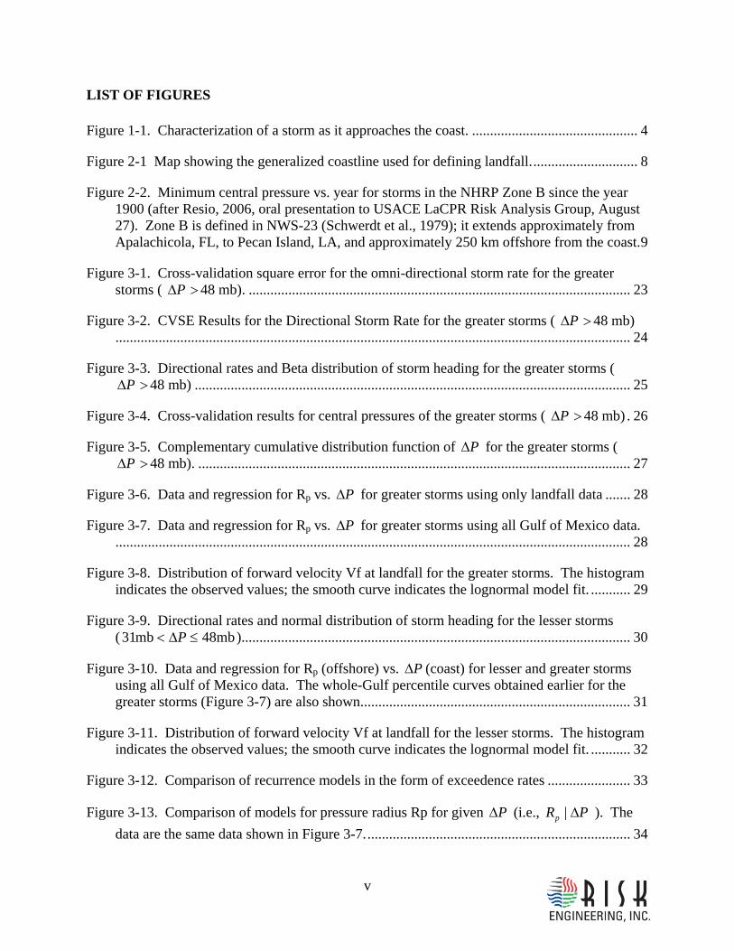
LIST OF FIGURES Figure 1-1. Characterization of a storm as it approaches the coast. .............................................. 4

Figure 2-1 Map showing the generalized coastline used for defining landfall.............................. 8

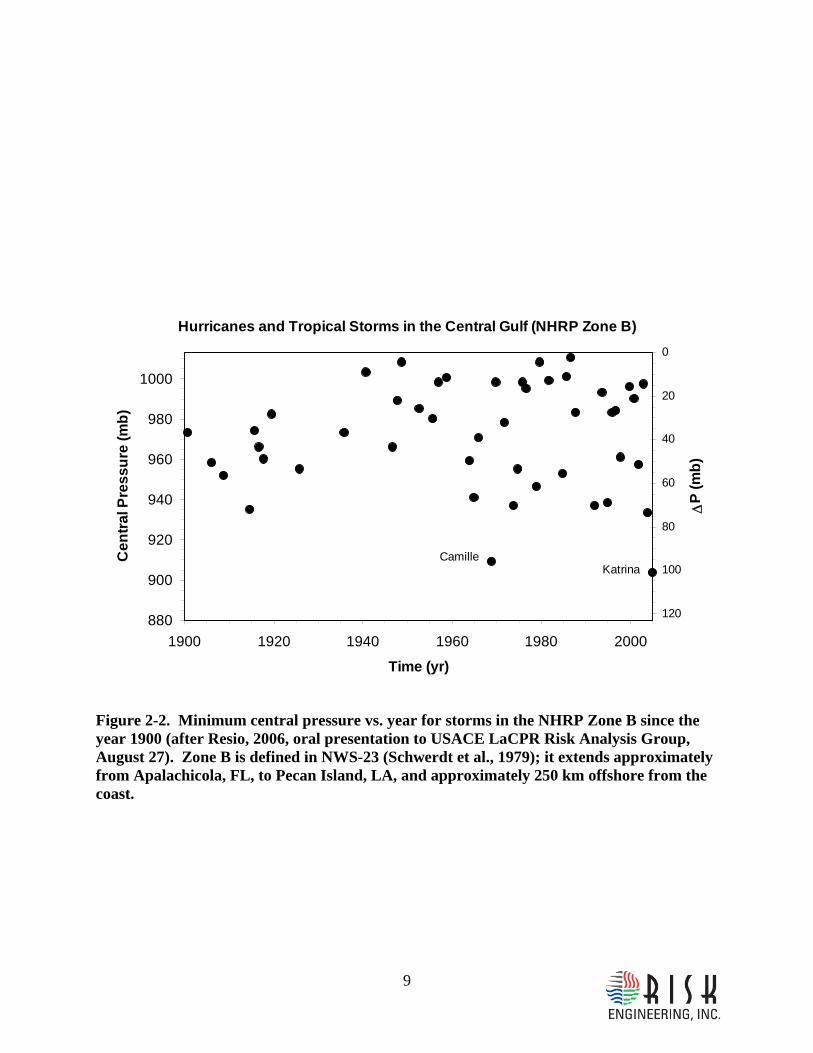
Figure 2-2. Minimum central pressure vs. year for storms in the NHRP Zone B since the year 1900 (after Resio, 2006, oral presentation to USACE LaCPR Risk Analysis Group, August 27). Zone B is defined in NWS-23 (Schwerdt et al., 1979); it extends approximately from Apalachicola, FL, to Pecan Island, LA, and approximately 250 km offshore from the coast.9

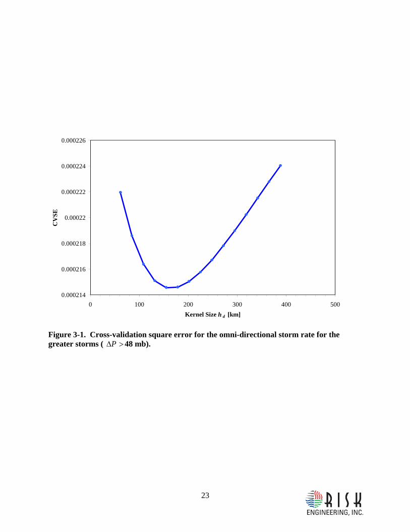
Figure 3-1. Cross-validation square error for the omni-directional storm rate for the greater storms ( >ΔP 48 mb). .......................................................................................................... 23

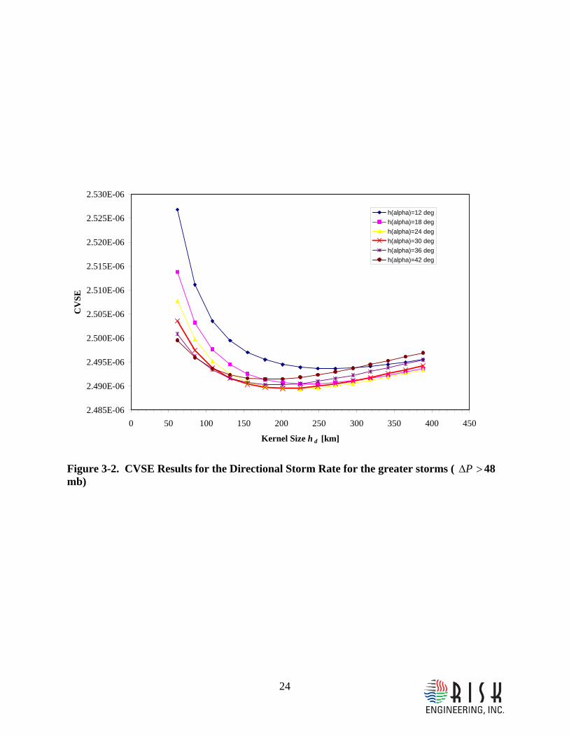
Figure 3-2. CVSE Results for the Directional Storm Rate for the greater storms ( >ΔP 48 mb)............................................................................................................................................... 24

Figure 3-3. Directional rates and Beta distribution of storm heading for the greater storms ( >ΔP 48 mb) ......................................................................................................................... 25

Figure 3-4. Cross-validation results for central pressures of the greater storms ( >ΔP 48 mb) . 26

Figure 3-5. Complementary cumulative distribution function of PΔ for the greater storms ( >ΔP 48 mb). ........................................................................................................................ 27

Figure 3-6. Data and regression for Rp vs. PΔ for greater storms using only landfall data ....... 28

Figure 3-7. Data and regression for Rp vs. PΔ for greater storms using all Gulf of Mexico data................................................................................................................................................ 28

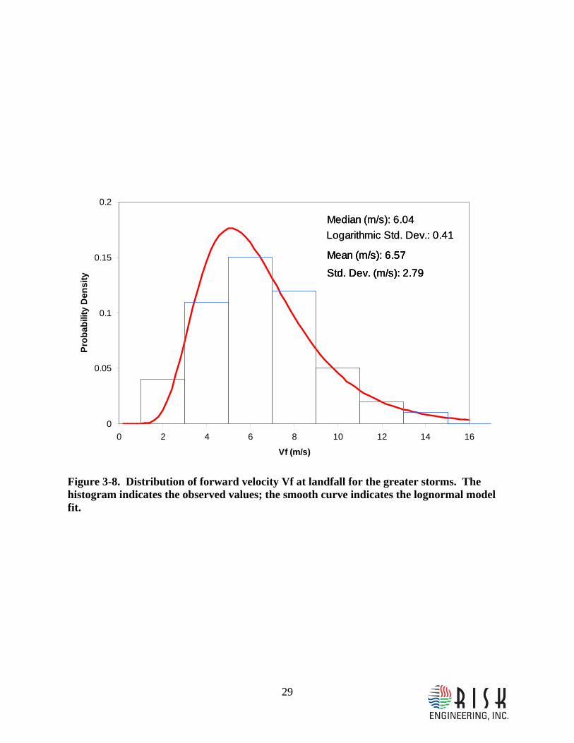
Figure 3-8. Distribution of forward velocity Vf at landfall for the greater storms. The histogram indicates the observed values; the smooth curve indicates the lognormal model fit. ........... 29

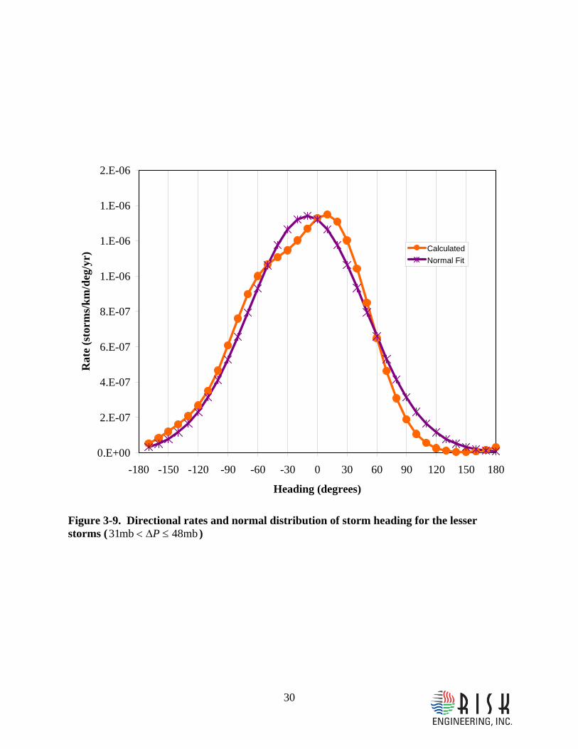
Figure 3-9. Directional rates and normal distribution of storm heading for the lesser storms ( mb48mb31 ≤Δ< P )............................................................................................................ 30

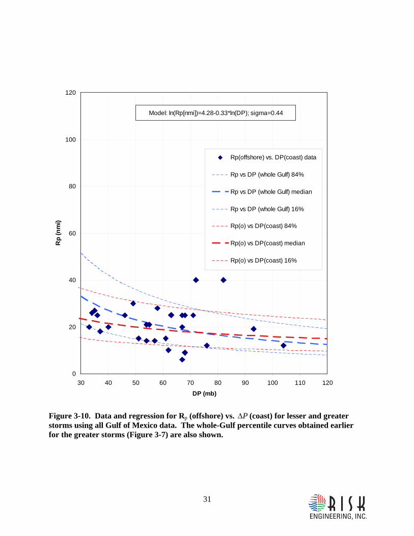
Figure 3-10. Data and regression for Rp (offshore) vs. PΔ (coast) for lesser and greater storms using all Gulf of Mexico data. The whole-Gulf percentile curves obtained earlier for the greater storms (Figure 3-7) are also shown........................................................................... 31

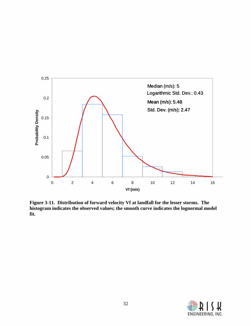
Figure 3-11. Distribution of forward velocity Vf at landfall for the lesser storms. The histogram indicates the observed values; the smooth curve indicates the lognormal model fit. ........... 32

Figure 3-12. Comparison of recurrence models in the form of exceedence rates ....................... 33

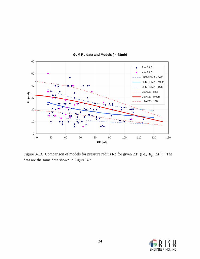
Figure 3-13. Comparison of models for pressure radius Rp for given PΔ (i.e., PRp Δ| ). The data are the same data shown in Figure 3-7.......................................................................... 34

vi

Figure 4-1. Illustration of the conditional distribution of random function )(xp at intermediate points between sampling nodes. The function )(xp has been sampled at 3 nodes 321 ,, xxx . The solid line displays the conditional mean value. The dashed lines display the conditional mean ± standard deviation range; the width of this range depends on the distance to the nodes and on the autocorrelation function ),( yxk . .............................................................. 53

Figure 4-2. Graphical representation of the JPM-OS 6 scheme for one landfall location. The areas of the circles are proportional to the associated annual rates. ..................................... 54

Figure 4-3. Validation of JPM-OS scheme for Lesser Storms. ................................................... 55

Figure 4-4. Map showing the tracks of the synthetic storms in the JPM-OS representation of the greater storms. Each small red square represents an hourly snapshot; size of the squares indicates PΔ . Note that this map shows only the master tracks (i.e., prior to offsetting their landfall locations). Note also that many of the synthetic storms follow identical or nearly identical tracks because they have identical or nearly identical values of θ (see Table 4-3)................................................................................................................................................ 56

Figure 4-5. Map showing the tracks of the synthetic storms in the JPM-OS representation of the lesser storms. Each small red square represents an hourly snapshot; size of the squares indicates PΔ . Note that this map shows only the master tracks (i.e., prior to offsetting their landfall locations).................................................................................................................. 57

Figure 4-6. Track and evolution of storm parameters for one synthetic storm. Source: OceanWeather....................................................................................................................... 58

vii

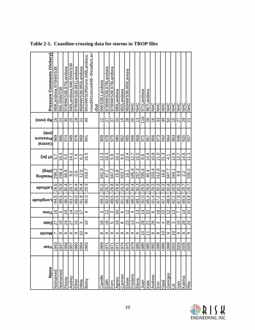
LIST OF TABLES Table 2-1. Coastline-crossing data for storms in TROP files ...................................................... 10

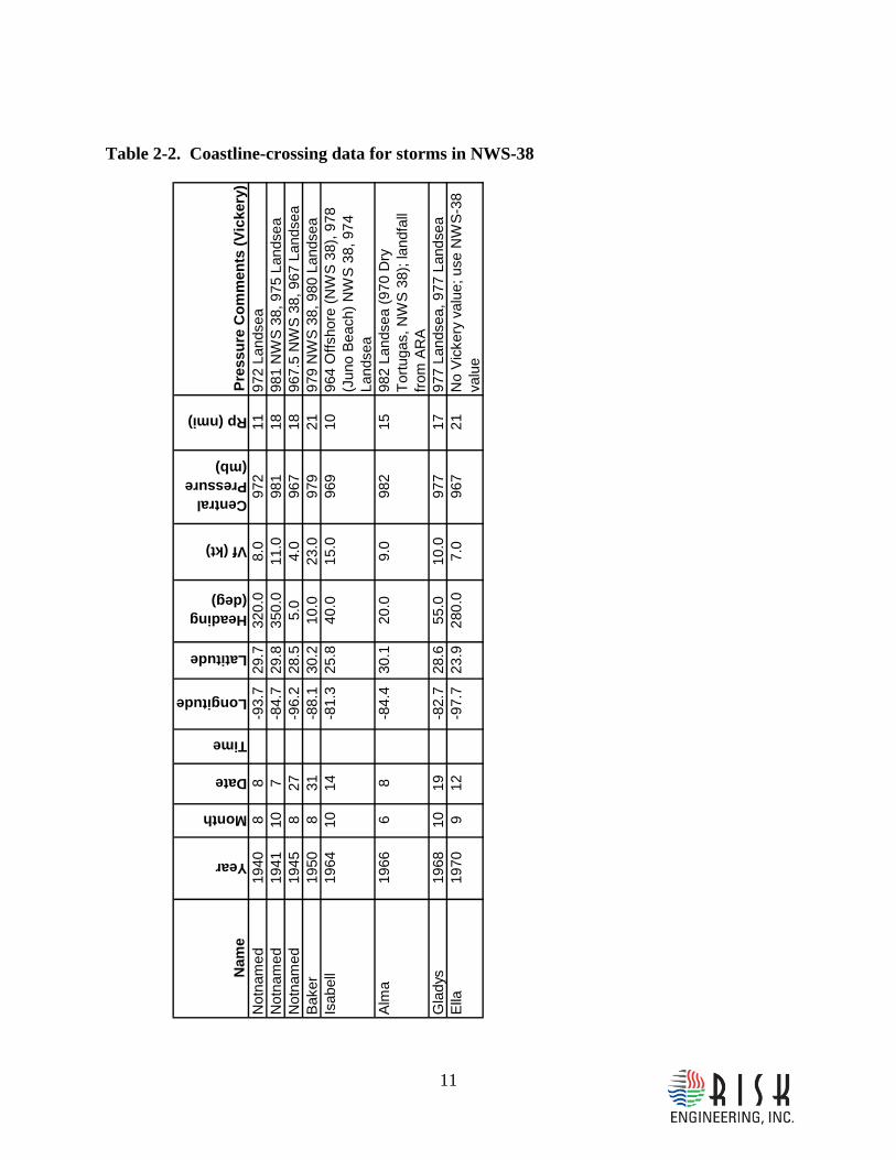
Table 2-2. Coastline-crossing data for storms in NWS-38 .......................................................... 11

Table 4-1. Discretization of PΔ into Slices in JPM-OS 6 Scheme for Greater Storms............. 50

Table 4-2. Correlation Distances in JPM-OS 6 Scheme for Greater Storms............................... 50

Table 4-3. Parameters of JPM-OS 6 scheme for the Greater Storms .......................................... 51

Table 4-4. Correlation Distances in JPM-OS Scheme for the Lesser Storms ............................. 52

Table 4-5. Parameters of JPM-OS scheme for the Lesser Storms............................................... 52

1

1 INTRODUCTION

1.1 PROJECT OBJECTIVES

The objective of this study is to provide the following two inputs for a Mississippi storm surge study being performed by the URS Group for FEMA:

1. A probabilistic characterization of the occurrence and characteristics of future1 hurricanes that may cause significant surge along the Mississippi coast.

2. A set of representative “Synthetic Storms,” and their associated recurrence rates, to be used for the numerical wind, wave, and surge calculations, and in the final probability calculations. These synthetic storms have characteristics and recurrence rates that make them representative of the entire population of possible future storms, for the purposes of surge-inundation calculations.

The numerical calculation of winds, waves, surge, and total inundation for these synthetic storms, the use of results from these calculations to compute elevations associated with exceedence probabilities of interest, and the actual results from these calculations are documented in URS (2007; we will refer to this report as the main URS report) report and in other contractor reports.

1.2 APPROACH The URS Mississippi surge study follows the Joint-Probability Method (JPM), as described by Resio (2007). This approach is analogous to the “deductive” approach utilized in the probabilistic analysis of hurricane-generated waves at offshore locations (Wen and Banon, 1991, 1988; Toro et al., 2004).

For the purposes of the JPM method, we describe the storm in terms of its characteristics as it reaches the coast in terms of the following parameters: the pressure deficit2 PΔ (representing hurricane intensity), the radius of the exponential pressure profile3 pR (representing hurricane

1 We refer to future storms, in the sense that risk analysis concerns itself with the future. On the other hand, it is important to keep in mind that we only consider the current climatological regime, as represented by the storm population considered in Section 2.

2 In this study, PΔ is calculated from the central pressure by assuming that the far-field pressure is always 1013 mb (i.e., CPP −=Δ 1013 ).

3 In this study, it is assumed that the radius of the exponential pressure profile pR and the radius to maximum winds maxR (sometimes written as RMW) are identical. This study will consider the values of pR both offshore and at the coast.

2

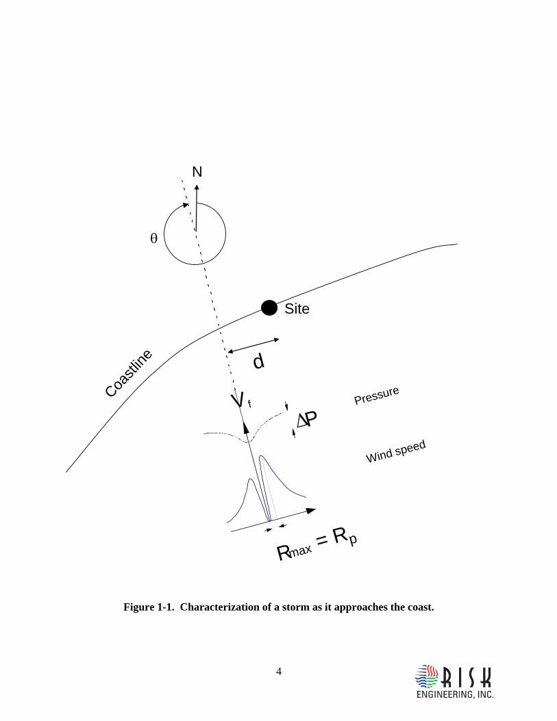
size), the forward velocity fV , the storm heading θ 4, and the landfall location (or, equivalently, the minimum distance from the track to a reference point along the coast). These parameters are illustrated in Figure 1-1. These parameters represent the main hurricane characteristics affecting storm surge; these parameters are treated as random variables in the JPM method. Other storm characteristics, including parameter B (Holland, 1980), are treated as constant at landfall or are not considered explicitly. Although hurricanes are much more complex than this parameterization allows for, and substantially more information is available for well-studied recent hurricanes, it is necessary at present to utilize this simple storm parameterization for the probabilistic characterization of future storms5.

It was decided to use the characteristics at landfall as the primary variables for the following two reasons: (1) most of the coastal surge is generated by the storm in the last 90 nautical miles prior to landfall (Resio, 2007), and (2) more and better hurricane data are available at the coast than offshore, especially for older storms.

For the statistical analyses to determine the storm recurrence rate and probability distribution of PΔ , which are the most important quantities in the storm characterization, we follow the

methodology developed by Chouinard and his co-workers (Chouinard, 1992; Chouinard and Liu, 1997; Chouinard et al., 1997). This methodology assigns weights to the historical hurricane data based on each hurricane’s distance to the site of interest, in a manner that provides an optimal compromise between statistical precision and geographical resolution. For other parameters, this study follows simpler statistical approaches.

The JPM method considers all possible combinations of storm characteristics at landfall, with their associated probabilities, calculates the surge effects for each combination, and then combines these results to obtain the annual probability of exceeding any desired storm stage. Mathematically, this calculation is represented as a multi-dimensional integral (the JPM integral).

Given the number of quantities affecting surge, and given the computational effort required to compute winds, waves, and surge for one combination of these quantities, a brute-force implementation of the JPM approach is not feasible. Two JPM-Optimal Sampling (JPM-OS) approaches have been developed to overcome this problem. The approach used in this study uses a quadrature procedure that approximates the multi-dimensional JPM integral by means of a weighted sum over a manageable number of discrete probability masses. Each of these masses may be interpreted as the characteristics at landfall of a representative synthetic storm. These characteristics, together with some simple deterministic rules, are then used to specify the entire storm history, which is then used as input to the numerical wind, wave, and surge models. Once the total inundation is computed for each synthetic storm, calculation of the associated

4 Direction to, measured clockwise from North.

5 The differences between real hurricanes and this simple parameterization are not ignored in the JPM formulation employed in this study. They are included in a statistical sense by means of the ε terms used in the JPM calculations, as will be explained in Section 4.2.

3

exceedence probabilities (or the inverse calculation of the surge associated with a certain exceedence probability) is straightforward.

The other JPM-OS approach performs wind, wave, and surge calculations for a set of carefully selected synthetic storms. The results from these calculations are then used to fit a parametric response surface, which is then used to evaluate the JPM integral numerically. See Resio (2007) for more details on this approach. A recent paper (Niedoroda et al., 2008) compares the two JPM-OS approaches and finds that the two approaches yield comparable results.

1.3 ORGANIZATION OF THIS REPORT Section 2 of this report documents the data used in this study. Section 3 documents the statistical analysis of these data to determine the storm rate and the probability distributions of PΔ , maxR ,

fV , and θ . Section 4 describes the JPM method in detail and documents the development of the quadrature procedure and the generation of synthetic storms.

4

Rmax

ΔPVf

d

Site

Coastl

ine

θ

= Rp

N

Wind speed

Pressure

Figure 1-1. Characterization of a storm as it approaches the coast.

5

2 DATA

2.1 INTRODUCTION This section documents the hurricane data to be used in Section 3 to develop the probabilistic model of hurricane occurrence and characteristics and discusses some of the key decisions that were necessary as part of the data collection and selection.

2.2 DATA SOURCES USED

This study considered only hurricanes with central pressures of 982 mb or lower (roughly corresponding in Category 2 and greater) at landfall. The hurricane data were further divided into lesser storms, with central pressures of 965 to 982 mb, and greater storms, with central pressures lower than 965 mb. Weaker hurricanes and tropical storms were deemed to make insignificant contribution to surge hazard, based on sensitivity studies.

The central pressures at landfall were obtained from a compilation provided by Dr. Peter Vickery of ARA, Inc. This compilation includes all hurricanes making landfall on the US Atlantic and Gulf of Mexico coast since 1900. For each hurricane, Vickery examined the central-pressure data from NOAA Technical Report NWS-38 (Ho et al., 1987; we will refer to this report as NWS-38 for the sake of brevity), NOAA Technical Memoranda TPC-1 and TPC-4, the NOAA HURDAT database, the “TROP” files provided by Oceanweather, Inc. (OWI), as well as other sources, and selected the most credible value. All other characteristics for the greater storms (and some of the lesser storms) were obtained from the TROP files. The characteristics obtained are the landfall central pressures, track coordinates, storm radius Rp, forward velocity of the storm center, and heading of the storm center (the latter two were derived from the coordinates and associated time stamps). These TROP files include all storms since 1940 that attained central pressures of 965 mb or less anywhere within the Gulf of Mexico.

Data for the radius, forward velocity, and heading of lesser storms not contained in the TROP files were obtained from NWS-38, which contains information for land falling hurricanes between 1900 and 1983. In addition, the HURDAT data set was scanned for data on lesser storms since 1983 which were not in the TROP files.

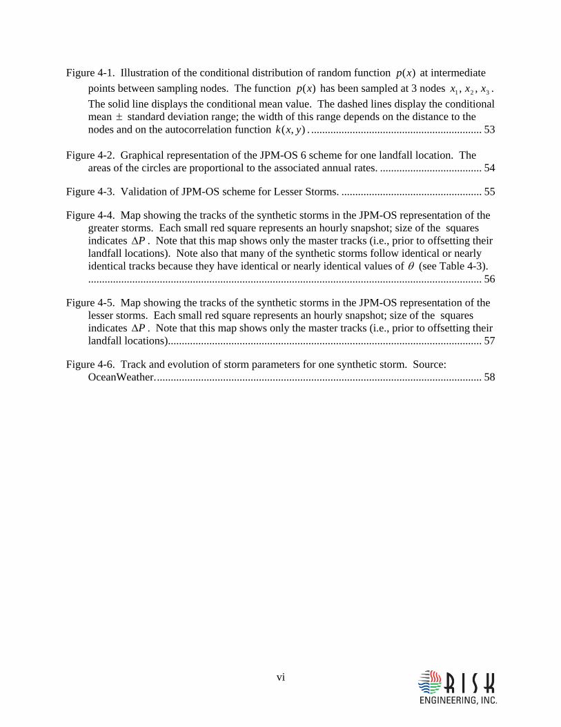
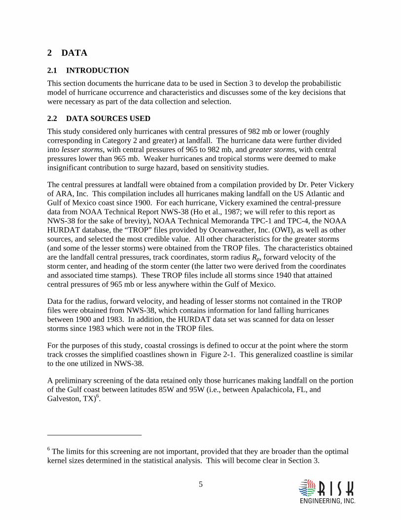
For the purposes of this study, coastal crossings is defined to occur at the point where the storm track crosses the simplified coastlines shown in Figure 2-1. This generalized coastline is similar to the one utilized in NWS-38.

A preliminary screening of the data retained only those hurricanes making landfall on the portion of the Gulf coast between latitudes 85W and 95W (i.e., between Apalachicola, FL, and Galveston, TX)6.

6 The limits for this screening are not important, provided that they are broader than the optimal kernel sizes determined in the statistical analysis. This will become clear in Section 3.

6

2.3 PERIOD OF RECORD

The selection of the time period to use as input for the statistical calculations is one of the most important decisions for an analysis of this kind. The TROP files available to this study extend back to 1940, but the NWS-38 and ARA data extend back to 1900. The HURDAT re-analysis data extend back to 1850, but they lack central-pressure data for many storms and do not contain the storm radius pR .

The problem of selecting the period of record may be stated as follows. On the one hand, we want to use as much of the available data as possible, in order to have the lowest possible statistical uncertainty in our probabilistic hurricane model of Section 3. On the other hand, we want to exclude older data that are incomplete or contain significant biases, in order to have a probabilistic model that is free of biases.

Although coastal and inland weather measurements improved steadily in quality and geographical coverage over the Twentieth Century, measurements were sparse and erratic until relatively recently. The older offshore data often depended on unplanned encounters by ships whose position relative to the storm was difficult to establish. This situation changed dramatically during World War II with the initiation of aircraft missions specifically designed to measure storm parameters. Since that time the quality of both offshore and onshore data has risen steadily. Aircraft instrumentation and navigation have increased in a more-or-less continuous fashion since World War II. Satellite observations were added during the 1960s, and these too have become increasingly more sophisticated and useful. There have been more instrument systems introduced in recent decades. Ocean data buoys with meteorological and oceanographic sensors have been deployed since the 1970s. A variety of Doppler radar installations has come online during the 1990s. Within the last few years mobile meteorological stations have been added to increase the spatial density of storm measurements.

Superimposed on this evolution in the observing system, there are natural large-scale atmospheric cycles, with periods of several years to decades, which may affect the rate and intensity of hurricanes (e.g., Gray, 1984; Webster et al., 2005; Bell and Chelliah, 2006; Resio and Orelup, 2006).

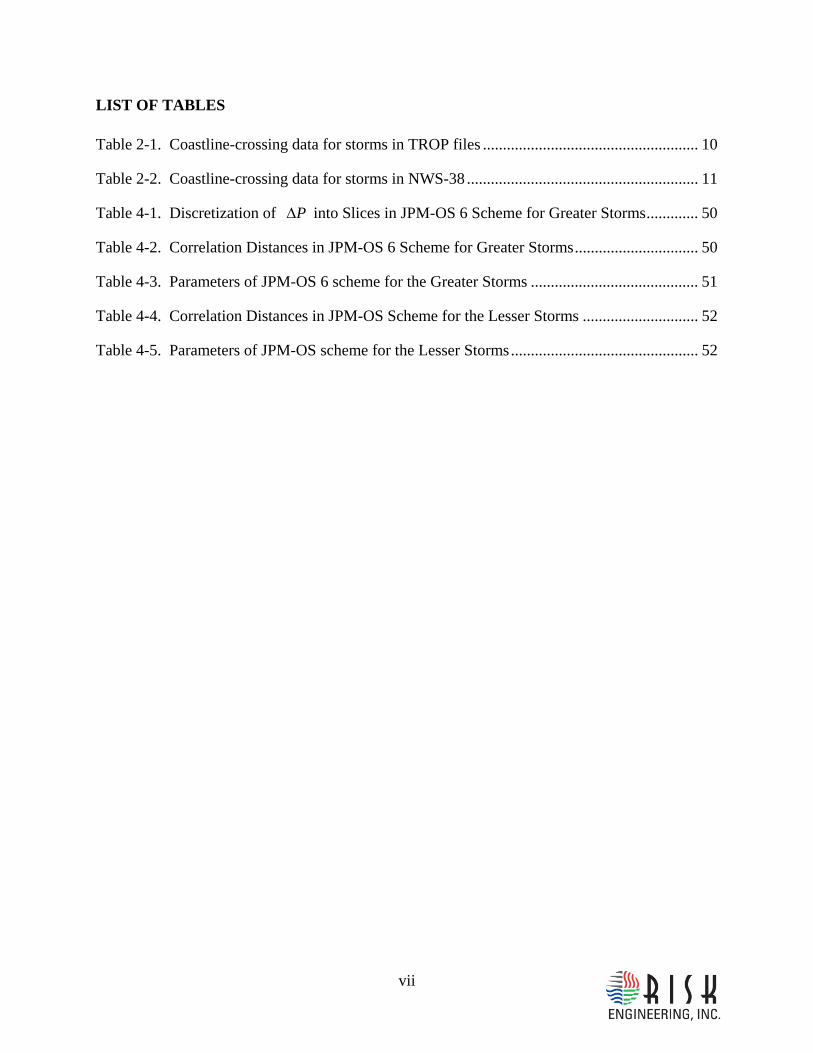
The combined effects of these two sets of factors may be seen in Figure 2-2, which shows the minimum central pressure by year for all tropical storms and hurricanes in the north-central Gulf of Mexico between the years 1900 and 2005. This figure suggests that fewer storms were detected in the first half of the 20th century. In particular, the figure suggests that some weak storms were not detected and that the intensity of some strong storms was underestimated. Cooper and Stear (2006) have also investigated this question and found significant differences between the first and second half oh the 20th century. Based on these considerations, it was decided to use the time period between 1940 and 2006 as the period of record for this study. Table 2-1 and Table 2-2 list the 1940-2006 coast-crossing data used.

Climate change and global warming are not considered in this study, largely because FEMA flood maps have a five-year shelf life and no significant effects are anticipated during this short time period. In addition, there is still considerable uncertainty about the effects of global warming on hurricane frequency and intensity (e.g., Holland and Webster, 2007; Gualdi et al.,

7

2008). The climate fluctuations and observed trends discussed above may also contain climate-change effects, but it is difficult to identify these effects at present.

8

100:W

100:W

95:W

95:W

90:W

90:W

85:W

85:W

80:W

80:W

20:N 20:N

25:N 25:N

30:N 30:N

Generalized Coastline

Figure 2-1 Map showing the generalized coastline used for defining landfall.

9

Hurricanes and Tropical Storms in the Central Gulf (NHRP Zone B)

880

900

920

940

960

980

1000

1900 1920 1940 1960 1980 2000

Time (yr)

Cen

tral P

ress

ure

(mb)

0

20

40

60

80

100

120

ΔP

(mb)

KatrinaCamille

Figure 2-2. Minimum central pressure vs. year for storms in the NHRP Zone B since the year 1900 (after Resio, 2006, oral presentation to USACE LaCPR Risk Analysis Group, August 27). Zone B is defined in NWS-23 (Schwerdt et al., 1979); it extends approximately from Apalachicola, FL, to Pecan Island, LA, and approximately 250 km offshore from the coast.

10

Table 2-1. Coastline-crossing data for storms in TROP files N

ame

Year

Month

Date

Time

Longitude

Latitude

Heading (deg)

Vf (kt)

Central Pressure (mb)

Rp (nmi)

Pres

sure

Com

men

ts (V

icke

ry)

Not

nam

ed19

437

2716

-94.

529

.529

6.2

5.7

969

1696

9Lan

dsea

,975

NW

S38

Not

nam

ed19

479

196

-89.

529

.929

8.4

16.4

966

2396

6.5N

WS3

8Fl

ossy

1956

924

24-8

6.5

30.4

66.8

9.0

974

3097

4NW

S38,

975L

ands

eaAu

drey

1957

627

14-9

3.7

29.7

9.0

14.1

945

2594

5Lan

dsea

,946

.5N

WS3

8Et

hel

1960

915

21-8

9.0

30.4

0.0

7.4

976

1897

6NW

S38,

981L

ands

eaH

ilda

1964

103

17-9

1.6

29.4

12.6

6.2

959

2195

9NW

S38,

950L

ands

eaBe

tsy

1965

910

4-9

0.3

29.3

316.

716

.594

140

941N

WSO

ffsho

re,9

48La

ndse

a,U

sed9

41si

nce9

48~3

hrsa

fterL

andf

all

Cam

ille19

698

183

-89.

330

.234

1.9

13.3

909

12N

WS3

8,La

ndse

aEd

ith19

719

1612

-92.

929

.747

.116

.397

827

978N

WS3

8,97

8Lan

dsea

Fern

1971

95

3-8

9.5

29.8

347.

25.

997

937

979N

WS3

8,97

9Lan

dsea

Agne

s19

726

1920

-85.

529

.915

.810

.198

020

980L

ands

eaC

arm

en19

749

86

-91.

229

.332

3.7

9.3

952

1595

2Lan

dsea

Eloi

se19

759

2312

-86.

230

.316

.123

.495

528

955N

WS3

8,95

5Lan

sea

Fred

eric

1979

913

4-8

8.3

30.4

345.

412

.794

625

NH

CEl

ena

1985

92

13-8

9.1

30.3

297.

315

.095

913

NH

CJu

an19

8510

2814

-92.

029

.529

5.6

8.6

971

116

971L

ands

eaKa

te19

8511

2122

-85.

429

.940

.414

.496

728

967L

ands

eaAn

drew

1992

826

8-9

1.4

29.3

333.

410

.995

616

NH

CEr

in19

958

316

-87.

230

.331

2.8

11.0

973

33N

HC

Opa

l19

9510

422

-87.

130

.318

.621

.394

239

NH

CG

eorg

es19

989

2812

-88.

930

.434

7.7

4.1

964

50N

HC

Lili

2002

103

13-9

2.2

29.5

344.

112

.996

315

NH

CIv

an20

049

167

-87.

930

.39.

812

.794

627

NH

CKa

trina

2005

829

14-8

9.6

29.7

2.2

14.6

920

29N

HC

Rita

2005

924

10-9

3.8

29.7

335.

211

.393

721

NH

C

11

Table 2-2. Coastline-crossing data for storms in NWS-38

Nam

e

Year

Month

Date

Time

Longitude

Latitude

Heading (deg)

Vf (kt)

Central Pressure (mb)

Rp (nmi)

Pres

sure

Com

men

ts (V

icke

ry)

Not

nam

ed19

408

8-9

3.7

29.7

320.

08.

097

211

972

Land

sea

Not

nam

ed19

4110

7-8

4.7

29.8

350.

011

.098

118

981

NW

S 38

, 975

Lan

dsea

Not

nam

ed19

458

27-9

6.2

28.5

5.0

4.0

967

1896

7.5

NW

S 38

, 967

Lan

dsea

Bake

r19

508

31-8

8.1

30.2

10.0

23.0

979

2197

9 N

WS

38, 9

80 L

ands

eaIs

abel

l19

6410

14-8

1.3

25.8

40.0

15.0

969

1096

4 O

ffsho

re (N

WS

38)

, 978

(J

uno

Beac

h) N

WS

38,

974

La

ndse

aAl

ma

1966

68

-84.

430

.120

.09.

098

215

982

Land

sea

(970

Dry

To

rtuga

s, N

WS

38);

land

fall

from

AR

AG

lady

s19

6810

19-8

2.7

28.6

55.0

10.0

977

1797

7 La

ndse

a, 9

77 L

ands

eaEl

la19

709

12-9

7.7

23.9

280.

07.

096

721

No

Vick

ery

valu

e; u

se N

WS-

38

valu

e

12

3 PROBABILISTIC MODEL OF STORM FREQUENCY AND CHARACTERISTICS (STORM CLIMATOLOGY)

3.1 INTRODUCTION This section documents the development of a probabilistic model for the occurrence and storm characteristics of hurricanes affecting the Mississippi Coast.

The occurrence of hurricanes in the neighborhood of a specific point is characterized by terms of the omni-directional rate )(xλ or the directional rate ),( θλ x using a Poisson line-process model (see Chouinard and Liu, 1997, for details).

The storm characteristics of interest are pressure deficit ( PΔ ), radius of maximum winds ( pR ), forward velocity ( fV ), distance to the point of interest x , and heading θ at landfall.

Because the East-West extent of the Mississippi Coast is only 120 km, it is reasonable to assume that the rate and probably distributions of the storm characteristics are constant within that length of coast and adjacent portions of the Louisiana coast. Therefore, the rate and probability distributions of the storm characteristics are defined for a single site (the Coastal Reference Point or CRP), with coordinates 30.20 N and 89.30 W. The CSR is located approximately 30 km (i.e., approximately one radius of maximum winds) west of the coastline midpoint, which is located approximately 30 km southwest of Gulfport, Mississippi.

For reasons related to project schedule and scope, we calculate separate rates and probabilistic models for the greater storms ( mbP 48>Δ ) and for the lesser storms ( mbPmb 4831 ≤Δ< ). Results for these two storm populations are described below.

3.2 CALCULATION OF STORM RATES FOR THE GREATER STORMS

3.2.1 Methodology and Optimal Kernel Sizes This study utilizes the methodology of Chouinard and Liu (1997; see also Chouinard, 1992) to calculate the rate of storms in the vicinity of the Coastal Reference Point. The geometry of storm tracks as they pass near a specific site is idealized as a Poisson line process. The key parameter of this model is the directional rate )(θλ 7. If direction is neglected, the key parameter is the omni-directional rate λ , which has units of storms/year/km.

The passage of each storm near a given site is characterized by the associated minimum distance d and storm heading θ of the storm relative to the site (see Figure 1-1). To calculate the rate at a site, Chouinard and Liu (1997) propose a kernel estimate, where the rate is proportional to a

7 Because we are considering a single site, namely the Coastal Reference Point, we will drop the argument x used earlier.

13

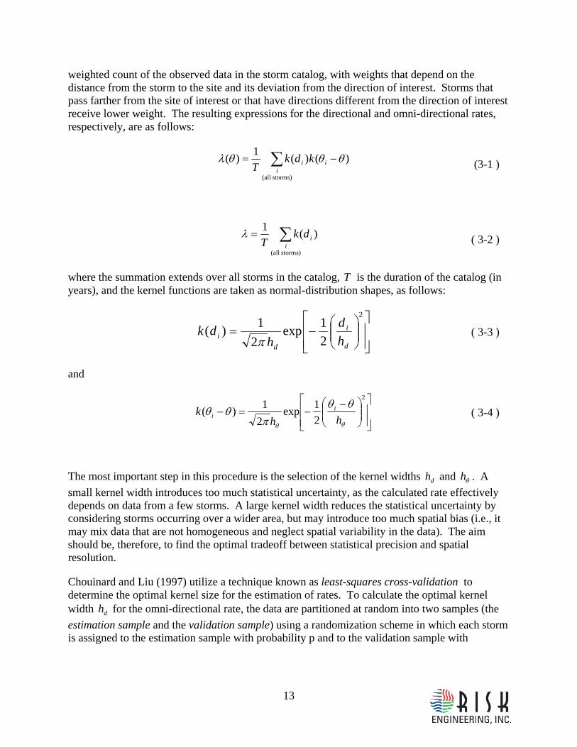
weighted count of the observed data in the storm catalog, with weights that depend on the distance from the storm to the site and its deviation from the direction of interest. Storms that pass farther from the site of interest or that have directions different from the direction of interest receive lower weight. The resulting expressions for the directional and omni-directional rates, respectively, are as follows:

∑ −=

storms)(all

)()(1)(i

ii kdkT

θθθλ (3-1 )

∑=

storms)(all

)(1i

idkT

λ ( 3-2 )

where the summation extends over all storms in the catalog, T is the duration of the catalog (in years), and the kernel functions are taken as normal-distribution shapes, as follows:

⎥⎥⎦

⎤

⎢⎢⎣

⎡⎟⎟⎠

⎞⎜⎜⎝

⎛−=

2

21exp

21)(

d

i

di h

dh

dkπ ( 3-3 )

and

⎥⎥⎦

⎤

⎢⎢⎣

⎡⎟⎟⎠

⎞⎜⎜⎝

⎛ −−=−

2

21exp

21)(

θθ

θθπ

θθhh

k ii ( 3-4 )

The most important step in this procedure is the selection of the kernel widths dh and θh . A small kernel width introduces too much statistical uncertainty, as the calculated rate effectively depends on data from a few storms. A large kernel width reduces the statistical uncertainty by considering storms occurring over a wider area, but may introduce too much spatial bias (i.e., it may mix data that are not homogeneous and neglect spatial variability in the data). The aim should be, therefore, to find the optimal tradeoff between statistical precision and spatial resolution.

Chouinard and Liu (1997) utilize a technique known as least-squares cross-validation to determine the optimal kernel size for the estimation of rates. To calculate the optimal kernel width dh for the omni-directional rate, the data are partitioned at random into two samples (the estimation sample and the validation sample) using a randomization scheme in which each storm is assigned to the estimation sample with probability p and to the validation sample with

14

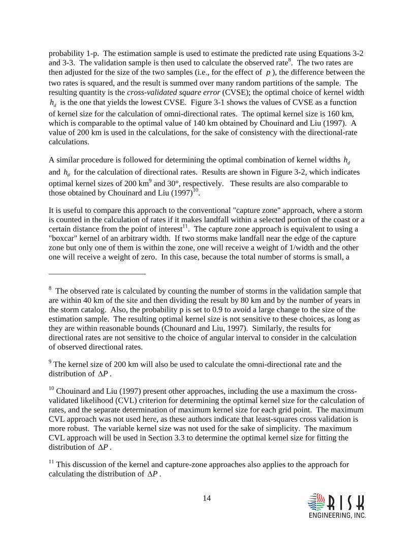
probability 1-p. The estimation sample is used to estimate the predicted rate using Equations 3-2 and 3-3. The validation sample is then used to calculate the observed rate8. The two rates are then adjusted for the size of the two samples (i.e., for the effect of p ), the difference between the two rates is squared, and the result is summed over many random partitions of the sample. The resulting quantity is the cross-validated square error (CVSE); the optimal choice of kernel width

dh is the one that yields the lowest CVSE. Figure 3-1 shows the values of CVSE as a function of kernel size for the calculation of omni-directional rates. The optimal kernel size is 160 km, which is comparable to the optimal value of 140 km obtained by Chouinard and Liu (1997). A value of 200 km is used in the calculations, for the sake of consistency with the directional-rate calculations.

A similar procedure is followed for determining the optimal combination of kernel widths dh and θh for the calculation of directional rates. Results are shown in Figure 3-2, which indicates optimal kernel sizes of 200 km9 and 30°, respectively. These results are also comparable to those obtained by Chouinard and Liu (1997)10.

It is useful to compare this approach to the conventional "capture zone" approach, where a storm is counted in the calculation of rates if it makes landfall within a selected portion of the coast or a certain distance from the point of interest11. The capture zone approach is equivalent to using a "boxcar" kernel of an arbitrary width. If two storms make landfall near the edge of the capture zone but only one of them is within the zone, one will receive a weight of 1/width and the other one will receive a weight of zero. In this case, because the total number of storms is small, a

8 The observed rate is calculated by counting the number of storms in the validation sample that are within 40 km of the site and then dividing the result by 80 km and by the number of years in the storm catalog. Also, the probability p is set to 0.9 to avoid a large change to the size of the estimation sample. The resulting optimal kernel size is not sensitive to these choices, as long as they are within reasonable bounds (Chounard and Liu, 1997). Similarly, the results for directional rates are not sensitive to the choice of angular interval to consider in the calculation of observed directional rates.

9 The kernel size of 200 km will also be used to calculate the omni-directional rate and the distribution of PΔ .

10 Chouinard and Liu (1997) present other approaches, including the use a maximum the cross-validated likelihood (CVL) criterion for determining the optimal kernel size for the calculation of rates, and the separate determination of maximum kernel size for each grid point. The maximum CVL approach was not used here, as these authors indicate that least-squares cross validation is more robust. The variable kernel size was not used for the sake of simplicity. The maximum CVL approach will be used in Section 3.3 to determine the optimal kernel size for fitting the distribution of PΔ .

11 This discussion of the kernel and capture-zone approaches also applies to the approach for calculating the distribution of PΔ .

15

small change in the size of the capture zone will lead to a large change in the calculated rate. In contrast, the Chouinard and Liu (1997) approach will give these two storms nearly identical weights. The two main differences between the Chouinard and Liu (1997) approach and the capture zone approach are as follows: (1) the smooth versus boxcar kernels, and (2) the objective versus arbitrary procedures to determine kernel size.

Another subtle issue relates to the definition of rates in terms of distance to the site of interest versus crossing of a line with a certain orientation. This study follows the former definition; recent US Army Corps of Engineers studies (e.g., Resio, 2007) follow the latter.

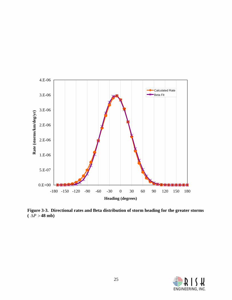
3.2.2 Results for Rate and for the Distribution of Heading Calculation of the omni-directional rate, using a kernel size of 200 km, yields a value of 2.88E-4 storms per year per kilometer, with a coefficient of variation of approximately 30%. Calculation of the directional rate, using kernel sizes of 200 km and 30°, yields the values shown in Figure 3-3.

Dividing the directional rate by the omni-directional rate, we obtain the probability distribution of the storm heading θ . This distribution is well approximated by a Beta distribution (also shown in Figure 3-3) with probability density function proportional to 11 )1( −− − tr xx , where

360/)180( += θx , 229.10=r , and 747.11=t . The associated mean and standard deviation are -12.4 degrees and 37.5 degrees, respectively.

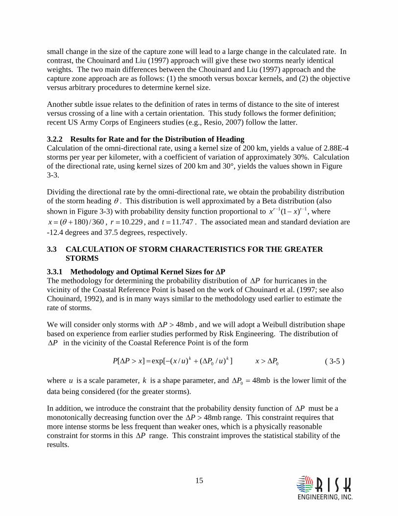
3.3 CALCULATION OF STORM CHARACTERISTICS FOR THE GREATER STORMS

3.3.1 Methodology and Optimal Kernel Sizes for ΔP The methodology for determining the probability distribution of PΔ for hurricanes in the vicinity of the Coastal Reference Point is based on the work of Chouinard et al. (1997; see also Chouinard, 1992), and is in many ways similar to the methodology used earlier to estimate the rate of storms.

We will consider only storms with mb48>ΔP , and we will adopt a Weibull distribution shape based on experience from earlier studies performed by Risk Engineering. The distribution of

PΔ in the vicinity of the Coastal Reference Point is of the form

00 ])/()/(exp[][ PxuPuxxPP kk Δ>Δ+−=>Δ ( 3-5 )

where u is a scale parameter, k is a shape parameter, and mb480 =ΔP is the lower limit of the data being considered (for the greater storms).

In addition, we introduce the constraint that the probability density function of PΔ must be a monotonically decreasing function over the mb48>ΔP range. This constraint requires that more intense storms be less frequent than weaker ones, which is a physically reasonable constraint for storms in this PΔ range. This constraint improves the statistical stability of the results.

16

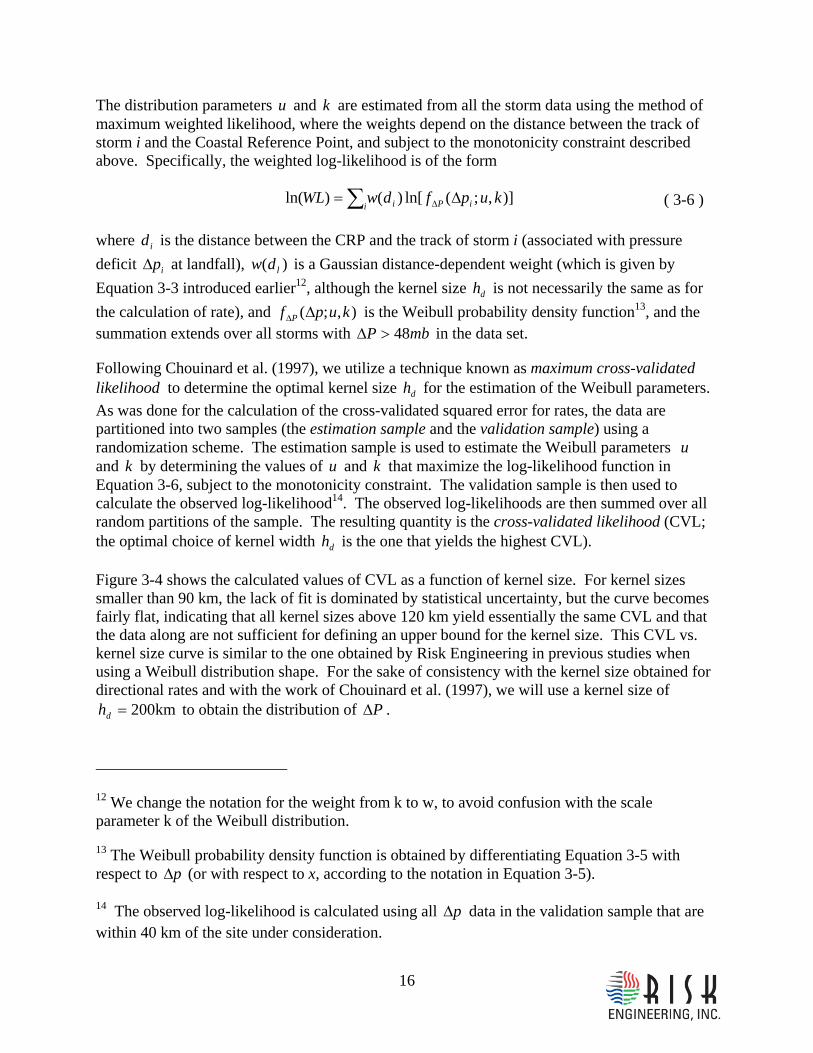
The distribution parameters u and k are estimated from all the storm data using the method of maximum weighted likelihood, where the weights depend on the distance between the track of storm i and the Coastal Reference Point, and subject to the monotonicity constraint described above. Specifically, the weighted log-likelihood is of the form

∑ Δ= Δi iPi kupfdwWL )],;(ln[)()ln( ( 3-6 )

where id is the distance between the CRP and the track of storm i (associated with pressure deficit ipΔ at landfall), )( ldw is a Gaussian distance-dependent weight (which is given by Equation 3-3 introduced earlier12, although the kernel size dh is not necessarily the same as for the calculation of rate), and ),;( kupf P ΔΔ is the Weibull probability density function13, and the summation extends over all storms with mbP 48>Δ in the data set.

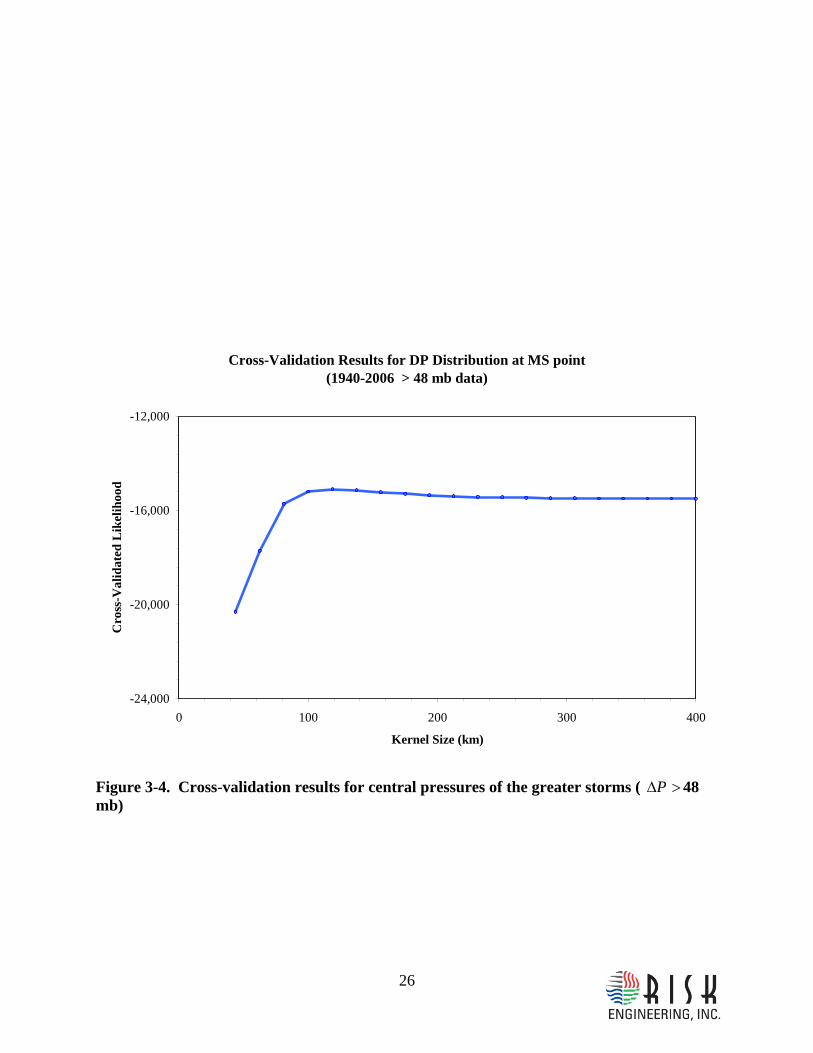
Following Chouinard et al. (1997), we utilize a technique known as maximum cross-validated likelihood to determine the optimal kernel size dh for the estimation of the Weibull parameters. As was done for the calculation of the cross-validated squared error for rates, the data are partitioned into two samples (the estimation sample and the validation sample) using a randomization scheme. The estimation sample is used to estimate the Weibull parameters u and k by determining the values of u and k that maximize the log-likelihood function in Equation 3-6, subject to the monotonicity constraint. The validation sample is then used to calculate the observed log-likelihood14. The observed log-likelihoods are then summed over all random partitions of the sample. The resulting quantity is the cross-validated likelihood (CVL; the optimal choice of kernel width dh is the one that yields the highest CVL).

Figure 3-4 shows the calculated values of CVL as a function of kernel size. For kernel sizes smaller than 90 km, the lack of fit is dominated by statistical uncertainty, but the curve becomes fairly flat, indicating that all kernel sizes above 120 km yield essentially the same CVL and that the data along are not sufficient for defining an upper bound for the kernel size. This CVL vs. kernel size curve is similar to the one obtained by Risk Engineering in previous studies when using a Weibull distribution shape. For the sake of consistency with the kernel size obtained for directional rates and with the work of Chouinard et al. (1997), we will use a kernel size of

km200=dh to obtain the distribution of PΔ .

12 We change the notation for the weight from k to w, to avoid confusion with the scale parameter k of the Weibull distribution.

13 The Weibull probability density function is obtained by differentiating Equation 3-5 with respect to pΔ (or with respect to x, according to the notation in Equation 3-5).

14 The observed log-likelihood is calculated using all pΔ data in the validation sample that are within 40 km of the site under consideration.

17

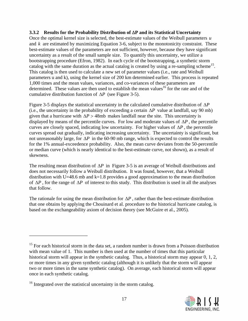
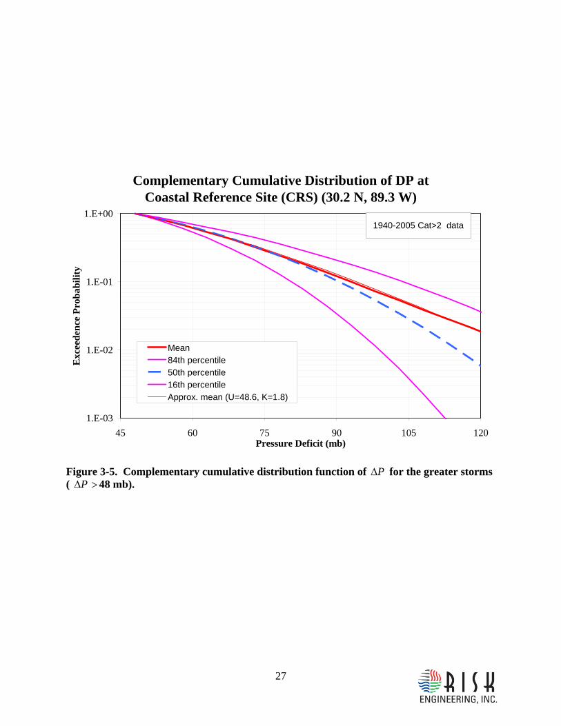
3.3.2 Results for the Probability Distribution of ΔP and its Statistical Uncertainty Once the optimal kernel size is selected, the best-estimate values of the Weibull parameters u and k are estimated by maximizing Equation 3-6, subject to the monotonicity constraint. These best-estimate values of the parameters are not sufficient, however, because they have significant uncertainty as a result of the small sample size. To quantify this uncertainty, we utilize a bootstrapping procedure (Efron, 1982). In each cycle of the bootstrapping, a synthetic storm catalog with the same duration as the actual catalog is created by using a re-sampling scheme15. This catalog is then used to calculate a new set of parameter values (i.e., rate and Weibull parameters u and k), using the kernel size of 200 km determined earlier. This process is repeated 1,000 times and the mean values, variances, and co-variances of these parameters are determined. These values are then used to establish the mean values16 for the rate and of the cumulative distribution function of PΔ (see Figure 3-5).

Figure 3-5 displays the statistical uncertainty in the calculated cumulative distribution of PΔ (i.e., the uncertainty in the probability of exceeding a certain PΔ value at landfall, say 90 mb) given that a hurricane with mb48>ΔP makes landfall near the site. This uncertainty is displayed by means of the percentile curves. For low and moderate values of PΔ , the percentile curves are closely spaced, indicating low uncertainty. For higher values of PΔ , the percentile curves spread out gradually, indicating increasing uncertainty. The uncertainty is significant, but not unreasonably large, for PΔ in the 60-90 mb range, which is expected to control the results for the 1% annual-exceedence probability. Also, the mean curve deviates from the 50-percentile or median curve (which is nearly identical to the best-estimate curve, not shown), as a result of skewness.

The resulting mean distribution of PΔ in Figure 3-5 is an average of Weibull distributions and does not necessarily follow a Weibull distribution. It was found, however, that a Weibull distribution with U=48.6 mb and k=1.8 provides a good approximation to the mean distribution of PΔ , for the range of PΔ of interest to this study. This distribution is used in all the analyses that follow.

The rationale for using the mean distribution for PΔ , rather than the best-estimate distribution that one obtains by applying the Chouinard et al. procedure to the historical hurricane catalog, is based on the exchangeability axiom of decision theory (see McGuire et al., 2005).

15 For each historical storm in the data set, a random number is drawn from a Poisson distribution with mean value of 1. This number is then used at the number of times that this particular historical storm will appear in the synthetic catalog. Thus, a historical storm may appear 0, 1, 2, or more times in any given synthetic catalog (although it is unlikely that the storm will appear two or more times in the same synthetic catalog). On average, each historical storm will appear once in each synthetic catalog.

16 Integrated over the statistical uncertainty in the storm catalog.

18

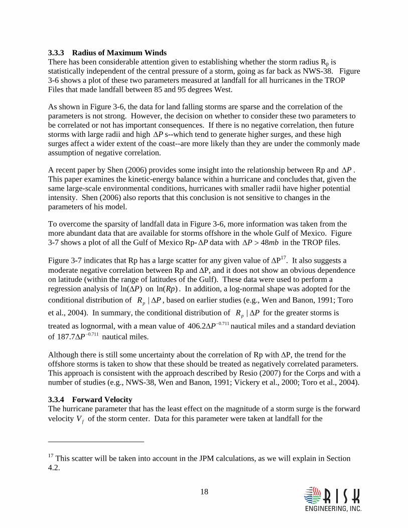
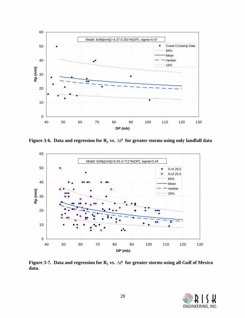
3.3.3 Radius of Maximum Winds There has been considerable attention given to establishing whether the storm radius Rp is statistically independent of the central pressure of a storm, going as far back as NWS-38. Figure 3-6 shows a plot of these two parameters measured at landfall for all hurricanes in the TROP Files that made landfall between 85 and 95 degrees West.

As shown in Figure 3-6, the data for land falling storms are sparse and the correlation of the parameters is not strong. However, the decision on whether to consider these two parameters to be correlated or not has important consequences. If there is no negative correlation, then future storms with large radii and high PΔ s--which tend to generate higher surges, and these high surges affect a wider extent of the coast--are more likely than they are under the commonly made assumption of negative correlation.

A recent paper by Shen (2006) provides some insight into the relationship between Rp and PΔ . This paper examines the kinetic-energy balance within a hurricane and concludes that, given the same large-scale environmental conditions, hurricanes with smaller radii have higher potential intensity. Shen (2006) also reports that this conclusion is not sensitive to changes in the parameters of his model.

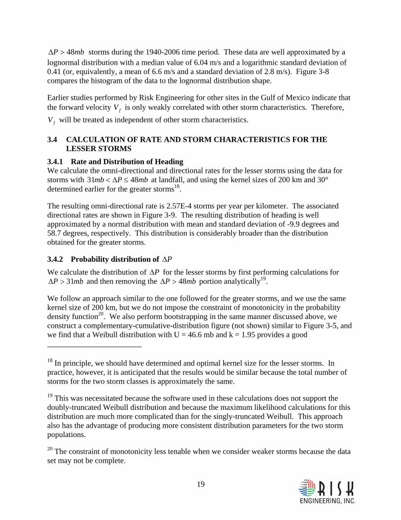
To overcome the sparsity of landfall data in Figure 3-6, more information was taken from the more abundant data that are available for storms offshore in the whole Gulf of Mexico. Figure 3-7 shows a plot of all the Gulf of Mexico Rp- PΔ data with mbP 48>Δ in the TROP files.

Figure 3-7 indicates that Rp has a large scatter for any given value of ΔP17. It also suggests a moderate negative correlation between Rp and ΔP, and it does not show an obvious dependence on latitude (within the range of latitudes of the Gulf). These data were used to perform a regression analysis of )ln( PΔ on )ln(Rp . In addition, a log-normal shape was adopted for the conditional distribution of PRp Δ| , based on earlier studies (e.g., Wen and Banon, 1991; Toro et al., 2004). In summary, the conditional distribution of PRp Δ| for the greater storms is

treated as lognormal, with a mean value of 711.02.406 −ΔP nautical miles and a standard deviation of 711.07.187 −ΔP nautical miles.

Although there is still some uncertainty about the correlation of Rp with ΔP, the trend for the offshore storms is taken to show that these should be treated as negatively correlated parameters. This approach is consistent with the approach described by Resio (2007) for the Corps and with a number of studies (e.g., NWS-38, Wen and Banon, 1991; Vickery et al., 2000; Toro et al., 2004).

3.3.4 Forward Velocity The hurricane parameter that has the least effect on the magnitude of a storm surge is the forward velocity fV of the storm center. Data for this parameter were taken at landfall for the

17 This scatter will be taken into account in the JPM calculations, as we will explain in Section 4.2.

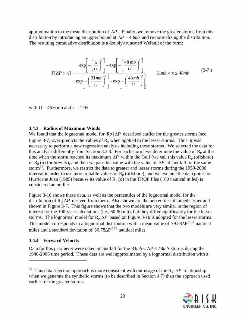
19

mbP 48>Δ storms during the 1940-2006 time period. These data are well approximated by a lognormal distribution with a median value of 6.04 m/s and a logarithmic standard deviation of 0.41 (or, equivalently, a mean of 6.6 m/s and a standard deviation of 2.8 m/s). Figure 3-8 compares the histogram of the data to the lognormal distribution shape.

Earlier studies performed by Risk Engineering for other sites in the Gulf of Mexico indicate that the forward velocity fV is only weakly correlated with other storm characteristics. Therefore,

fV will be treated as independent of other storm characteristics.

3.4 CALCULATION OF RATE AND STORM CHARACTERISTICS FOR THE LESSER STORMS

3.4.1 Rate and Distribution of Heading We calculate the omni-directional and directional rates for the lesser storms using the data for storms with mbPmb 4831 ≤Δ< at landfall, and using the kernel sizes of 200 km and 30° determined earlier for the greater storms18.

The resulting omni-directional rate is 2.57E-4 storms per year per kilometer. The associated directional rates are shown in Figure 3-9. The resulting distribution of heading is well approximated by a normal distribution with mean and standard deviation of -9.9 degrees and 58.7 degrees, respectively. This distribution is considerably broader than the distribution obtained for the greater storms.

3.4.2 Probability distribution of PΔ We calculate the distribution of PΔ for the lesser storms by first performing calculations for

mbP 31>Δ and then removing the mbP 48>Δ portion analytically19.

We follow an approach similar to the one followed for the greater storms, and we use the same kernel size of 200 km, but we do not impose the constraint of monotonicity in the probability density function20. We also perform bootstrapping in the same manner discussed above, we construct a complementary-cumulative-distribution figure (not shown) similar to Figure 3-5, and we find that a Weibull distribution with U = 46.6 mb and k = 1.95 provides a good

18 In principle, we should have determined and optimal kernel size for the lesser storms. In practice, however, it is anticipated that the results would be similar because the total number of storms for the two storm classes is approximately the same.

19 This was necessitated because the software used in these calculations does not support the doubly-truncated Weibull distribution and because the maximum likelihood calculations for this distribution are much more complicated than for the singly-truncated Weibull. This approach also has the advantage of producing more consistent distribution parameters for the two storm populations.

20 The constraint of monotonicity less tenable when we consider weaker storms because the data set may not be complete.

20

approximation to the mean distribution of PΔ . Finally, we remove the greater storms from this distribution by introducing an upper bound at mbP 48=Δ and re-normalizing the distribution. The resulting cumulative distribution is a doubly-truncated Weibull of the form:

mbxmb

Umb

Umb

Umb

Ux

xPPkk

kk

483148exp31exp

48expexp

][ ≤<

⎥⎥⎦

⎤

⎢⎢⎣

⎡⎟⎠⎞

⎜⎝⎛−−

⎥⎥⎦

⎤

⎢⎢⎣

⎡⎟⎠⎞

⎜⎝⎛−

⎥⎥⎦

⎤

⎢⎢⎣

⎡⎟⎠⎞

⎜⎝⎛−−

⎥⎥⎦

⎤

⎢⎢⎣

⎡⎟⎠⎞

⎜⎝⎛−

=>Δ (3-7 )

with U = 46.6 mb and k = 1.95.

3.4.3 Radius of Maximum Winds We found that the lognormal model for PRp Δ| described earlier for the greater storms (see Figure 3-7) over-predicts the values of Rp when applied to the lesser storms. Thus, it was necessary to perform a new regression analysis including these storms. We selected the data for this analysis differently from Section 3.3.3. For each storm, we determine the value of Rp at the time when the storm reached its maximum PΔ within the Gulf (we call this value Rp (offshore) or Rp (o) for brevity), and then we pair this value with the value of PΔ at landfall for the same storm21. Furthermore, we restrict the data to greater and lesser storms during the 1950-2006 interval in order to use more reliable values of Rp (offshore), and we exclude the data point for Hurricane Juan (1985) because its value of Rp (o) in the TROP files (100 nautical miles) is considered an outlier.

Figure 3-10 shows these data, as well as the percentiles of the lognormal model for the distribution of Rp| PΔ derived from them. Also shown are the percentiles obtained earlier and shown in Figure 3-7. This figure shows that the two models are very similar in the region of interest for the 100-year calculations (i.e., 60-90 mb), but they differ significantly for the lesser storms. The lognormal model for Rp| PΔ based on Figure 3-10 is adopted for the lesser storms. This model corresponds to a lognormal distribution with a mean value of -0.33P79.58Δ nautical miles and a standard deviation of -0.33P36.78Δ nautical miles.

3.4.4 Forward Velocity

Data for this parameter were taken at landfall for the mbPmb 4831 ≤Δ< storms during the 1940-2006 time period. These data are well approximated by a lognormal distribution with a

21 This data selection approach is more consistent with our usage of the Rp- PΔ relationship when we generate the synthetic storms (to be described in Section 4.7) than the approach used earlier for the greater storms.

21

median value of 5.0 m/s and a logarithmic standard deviation of 0.43 (or, equivalently, a mean of 5.5 m/s and a standard deviation of 2.5 m/s; i.e., slightly slower than the greater storms). Figure 3-11 compares the histogram of the data to the lognormal distribution shape.

3.5 COMPARISON TO THE CORPS MSCIP PROJECT It is useful to compare the probabilistic model of hurricane occurrence and characteristics developed in this section to the one developed by the Army Corps of Engineers ERDC for the same region as part of the Mississippi Coastal Improvement Project (MsCIP). Because the

PΔ exceedence rates (i.e., the product of the rate and the distribution function of PΔ ) and the distribution of pressure radius Rp (more precisely, the conditional distribution of PRp Δ| ) constitute the most important elements of the probabilistic model, this comparison will be restricted to these two quantities.

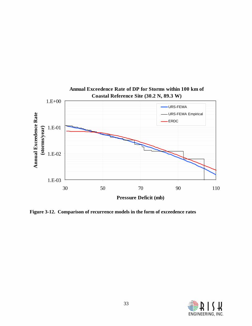
Figure 3-12 compares the results in the form of annual exceedence rates. All the rates are multiplied by a length of 200 km to obtain the exceedence rates for storms passing within 100 km of the site (on either side). The results from this study (labeled URS-FEMA) contain both the lesser and greater storms. The results from the Corps of Engineers (labeled ERDC) are computed on the basis of parameters provided by Resio (personal communication, 2007). Also shown is the empirical distribution (labeled URS-FEMA Empirical),which is computed from the 1940-2006 data, after applying distance-dependent weights based on a 200-km kernel size. This comparison shows a good agreement.

Figure 3-13 compares the mean and percentile curves of the distributions of PRp Δ| . There are some differences between the curves at intermediate values of PΔ , with the ERDC model having a tendency for larger storms. These differences are mainly the result of different choices for functional-forms and distribution shapes, and are difficult to resolve with existing data.

3.6 SUMMARY This section documents the development of the probabilistic model for the occurrence and characteristics of future hurricanes that may generate significant storm surge along the Mississippi coast. Because the rate and model parameters vary little over the 100 km of Mississippi coast, it is appropriate to neglect this variation and perform the analysis for a single point.

The storm population is partitioned into greater and lesser storms, and separate models are computed for both. For each storm population, the following parameters were estimated: annual occurrence rate, probability distribution of pressure deficit PΔ , conditional probability distribution of storm size (as measured by Rp) given PΔ , probability distribution of forward velocity, and probability distribution of storm heading θ . The observation that the storm rate does not vary along the coast and adjacent portions of Louisiana, implies a uniform distribution of (perpendicular) distance to any site of interest.

22

Other characteristics of hurricanes are not included explicitly in this parameterization. The effect of these characteristics on the exceedence probabilities will be included in an approximate manner by means of a random error term.

The following is a summary of the distributions and parameter values obtained.

a. Rate( PΔ >48 mb) = 2.88E-4E-4 storms/km/yr Rate ( PΔ 31-48 mb) = 2.57E-4 storms/km/yr

Can treat distance as uniformly distributed b. Heading:

i. PΔ >48 mb, Beta ( 229.10=r , and 747.11=t ) ii. PΔ 31-48 mb, normal (mean= -9.9 deg, σ =58.7 deg; truncate at 90± degrees)

c. PΔ : three-parameter Weibull i. PΔ >48 mb, U = 48.6 mb, k = 1.8 (see Equation ( 3-5 ))

ii. PΔ 31-48 mb, U = 46.6 mb, k = 1.95 (see Equation (3-7 )) d. Rp given PΔ : lognormal

i. Greater storms 1. mean (nmi): 711.02.406 −ΔP 2. sigma (nmi): 711.07.187 −ΔP

ii. Lesser storms 1. mean (nmi): -0.33P79.58Δ 2. sigma (nmi): -0.33P36.78Δ

e. Vf: lognormal i. Greater storms

1. mean (m/s); 6.6 2. sigma (m/s): 2.8

ii. Lesser storms 1. mean (m/s); 5.5 2. sigma (m/s): 2.5

These parameters will be utilized in Section 4 to generate a set of representative synthetic storms, using a JPM-OS formulation.

23

0.000214

0.000216

0.000218

0.00022

0.000222

0.000224

0.000226

0 100 200 300 400 500Kernel Size h d [km]

CV

SE

Figure 3-1. Cross-validation square error for the omni-directional storm rate for the greater storms ( >ΔP 48 mb).

24

2.485E-06

2.490E-06

2.495E-06

2.500E-06

2.505E-06

2.510E-06

2.515E-06

2.520E-06

2.525E-06

2.530E-06

0 50 100 150 200 250 300 350 400 450

Kernel Size h d [km]

CV

SE

h(alpha)=12 degh(alpha)=18 degh(alpha)=24 degh(alpha)=30 degh(alpha)=36 degh(alpha)=42 deg

Figure 3-2. CVSE Results for the Directional Storm Rate for the greater storms ( >ΔP 48 mb)

25

0.E+00

5.E-07

1.E-06

2.E-06

2.E-06

3.E-06

3.E-06

4.E-06

-180 -150 -120 -90 -60 -30 0 30 60 90 120 150 180

Heading (degrees)

Rat

e (s

torm

s/km

/deg

/yr)

Calculated RateBeta Fit

Figure 3-3. Directional rates and Beta distribution of storm heading for the greater storms ( >ΔP 48 mb)

26

Cross-Validation Results for DP Distribution at MS point (1940-2006 > 48 mb data)

-24,000

-20,000

-16,000

-12,000

0 100 200 300 400

Kernel Size (km)

Cro

ss-V

alid

ated

Lik

elih

ood

Figure 3-4. Cross-validation results for central pressures of the greater storms ( >ΔP 48 mb)

27

Complementary Cumulative Distribution of DP at Coastal Reference Site (CRS) (30.2 N, 89.3 W)

1.E-03

1.E-02

1.E-01

1.E+00

45 60 75 90 105 120Pressure Deficit (mb)

Exc

eede

nce

Prob

abili

ty

Mean84th percentile50th percentile16th percentileApprox. mean (U=48.6, K=1.8)

1940-2005 Cat>2 data

Figure 3-5. Complementary cumulative distribution function of PΔ for the greater storms ( >ΔP 48 mb).

28

0

10

20

30

40

50

60

40 50 60 70 80 90 100 110 120 130

DP (mb)

Rp

(nm

i)

Coast-Crossing Data84%Meanmedian16%

Model: ln(Rp[nmi])=4.37-0.291*ln(DP); sigma=0.47

Figure 3-6. Data and regression for Rp vs. PΔ for greater storms using only landfall data

0

10

20

30

40

50

60

40 50 60 70 80 90 100 110 120 130

DP (mb)

Rp

(nm

i)

S of 29.5N of 29.584%Meanmedian16%

Model: ln(Rp[nmi])=5.91-0.711*ln(DP); sigma=0.44

Figure 3-7. Data and regression for Rp vs. PΔ for greater storms using all Gulf of Mexico data.

29

0

0.05

0.1

0.15

0.2

0 2 4 6 8 10 12 14 16

Vf (m/s)

Prob

abili

ty D

ensi

ty

Median (m/s): 6.04Logarithmic Std. Dev.: 0.41

Mean (m/s): 6.57

Std. Dev. (m/s): 2.79

Mean (m/s): 6.57

Std. Dev. (m/s): 2.79

Median (m/s): 6.04Logarithmic Std. Dev.: 0.41

Mean (m/s): 6.57

Std. Dev. (m/s): 2.79

Figure 3-8. Distribution of forward velocity Vf at landfall for the greater storms. The histogram indicates the observed values; the smooth curve indicates the lognormal model fit.

30

0.E+00

2.E-07

4.E-07

6.E-07

8.E-07

1.E-06

1.E-06

1.E-06

2.E-06

-180 -150 -120 -90 -60 -30 0 30 60 90 120 150 180

Heading (degrees)

Rat

e (s

torm

s/km

/deg

/yr)

CalculatedNormal Fit

Figure 3-9. Directional rates and normal distribution of storm heading for the lesser storms ( mb48mb31 ≤Δ< P )

31

0

20

40

60

80

100

120

30 40 50 60 70 80 90 100 110 120

DP (mb)

Rp

(nm

i)

Rp(offshore) vs. DP(coast) data

Rp vs DP (whole Gulf) 84%

Rp vs DP (whole Gulf) median

Rp vs DP (whole Gulf) 16%

Rp(o) vs DP(coast) 84%

Rp(o) vs DP(coast) median

Rp(o) vs DP(coast) 16%

Model: ln(Rp[nmi])=4.28-0.33*ln(DP); sigma=0.44

M

Figure 3-10. Data and regression for Rp (offshore) vs. PΔ (coast) for lesser and greater storms using all Gulf of Mexico data. The whole-Gulf percentile curves obtained earlier for the greater storms (Figure 3-7) are also shown.

32

0

0.05

0.1

0.15

0.2

0.25

0 2 4 6 8 10 12 14 16

Vf (m/s)

Prob

abili

ty D

ensi

ty

Median (m/s): 5Logarithmic Std. Dev.: 0.43

Mean (m/s): 5.48

Std. Dev. (m/s): 2.47

Mean (m/s): 5.48

Std. Dev. (m/s): 2.47

Median (m/s): 5Logarithmic Std. Dev.: 0.43

Mean (m/s): 5.48

Std. Dev. (m/s): 2.47

Figure 3-11. Distribution of forward velocity Vf at landfall for the lesser storms. The histogram indicates the observed values; the smooth curve indicates the lognormal model fit.

33

Annual Exceedence Rate of DP for Storms within 100 km of Coastal Reference Site (30.2 N, 89.3 W)

1.E-03

1.E-02

1.E-01

1.E+00

30 50 70 90 110

Pressure Deficit (mb)

Ann

ual E

xcee

denc

e R

ate

(sto

rms/y

ear)

URS-FEMA

URS-FEMA Empirical

ERDC

Figure 3-12. Comparison of recurrence models in the form of exceedence rates

34

GoM Rp data and Models (>=48mb)

0

10

20

30

40

50

60

40 50 60 70 80 90 100 110 120 130

DP (mb)

Rp

(nm

i)

S of 29.5

N of 29.5

URS-FEMA - 84%

URS-FEMA - Mean

URS-FEMA - 16%

USACE - 84%

USACE - Mean

USACE - 16%

Figure 3-13. Comparison of models for pressure radius Rp for given PΔ (i.e., PRp Δ| ). The data are the same data shown in Figure 3-7.

35

4 DEVELOPMENT AND IMPLEMENTATION OF JPM-OS APPROACH, INCLUDING THE DEVELOPMENT OF SYNTHETIC STORMS

4.1 INTRODUCTION This section documents the development of a set of representative synthetic storms and their associated annual recurrence rates. These storms, together with their rates, provide a condensed representation of the population of possible future synthetic storms, for use in the calculation of surge inundation probabilities.

The section begins by describing the JPM method, including the rationale for the error terms that account for un-modeled parameters and effects. This is followed by a general description of the Quadrature JPM-OS approach adopted in this study, a detailed description of the Bayesian Quadrature method, and implementation details. The section concludes with a description of the procedure followed to generate synthetic storms from the storm characteristics at landfall.

4.2 THE JOINT PROBABILITY METHOD The Joint Probability Method or JPM was developed for coastal storm surge studies by Myers (Myers, 1975; Ho and Meyers, 1975). JPM provides a mathematical framework for the calculation of surge exceedence probabilities in terms of the hurricane climatology and hurricane surge effects. In particular, the JPM approach combines the following inputs:

• The annual rate of storms of interest λ . For this study, storms of interest are defined as hurricanes with mbP 31>Δ making landfall on or within approximately 30 km of the Mississippi coast. Typically, it is also assumed that the occurrences of these storms in time represents a Poisson random process (Parzen, 1962)23.

• The joint probability distribution )(xfX of the storm characteristics for storms of interest. These characteristics are defined very broadly at first, but they are narrowed later to make the approach practical.

• The storm-generated surge24 )(Xη at the site of interest, given the storm characteristics.

The combined effect of these three inputs is expressed by the multiple integral

23 In practice, the Poisson assumption is not necessary. Weaker assumptions are sufficient when calculating the probabilities of rare events, as will be discussed below.

24 In this definition, the term surge represents the peak total inundation, including the surge itself, wave setup, astronomical tide, etc.

36

∫∫ >=>x Xyr xdxPxfP ])([)(...][ )1max( ηηληη (4-1 )

where ])([ ηη >xP is the conditional probability that a storm of certain characteristics x will generate a flood elevation in excess of an arbitrary value η . This probability would be a Heaviside step function )]([ XH ηη − if vector X contained a complete characterization of the storm and if the numerical models for the calculation of surge given x were perfect, but these conditions cannot be satisfied in practice. The integral above considers all possible storm characteristics from the population of storms of interest and calculates the fraction of these storms that produce surges in excess of the value of interest η , using the total probability theorem (Benjamin and Cornell, 1970).

The right hand side in Equation 4-1 actually represents the mean annual rate of storms that exceed η at the site, but it also provides a good approximation to the annual exceedence probability25.

Equation 4-1 defines a smooth function of η that can be used to determine the flood levels associated with any annual probability of exceedence. Those of interest in this study are the 10%, 2%, 1% and 0.2 % annual probabilities. These are often referred to as the 10-, 50-, 100- and 500-yr annual exceedence levels, respectively. Unfortunately, the concept of return periods is often misunderstood.

As noted by Resio (2007), some approximations are necessary in practice for the evaluation of Equation 4-1. Firstly, it would be impossible to calculate the peak surge exactly, even if the storm’s wind field as a function of time was known exactly. To this effect, we write the actual elevation )(Xη in terms of the model-calculated elevation )(Xmη as mm XX εηη += )()( , where mε is a modeling-error term, which will be treated as a random quantity independent of X . If the model is unbiased, mε has a mean value of zero. Using the above representation, one can write the actual conditional probability as ])([ ηη >xP as

])([])([ ηεηηη >+=> mm XPXP (4-2 )

25 The derivation to show that the annual probability for a rare event is approximately equal to annual rate is usually made by assuming that event occurrences represent a Poisson process and then linearizing the resulting exponential. The same result may be obtained under weaker assumptions; it is sufficient to assume that the probability of two or more of these rare events in one year is much lower than the probability of one event. This condition is satisfied for hurricane-generated surges and for the exceedence probabilities of interest in this study (e.g, 0.01 per year).

37

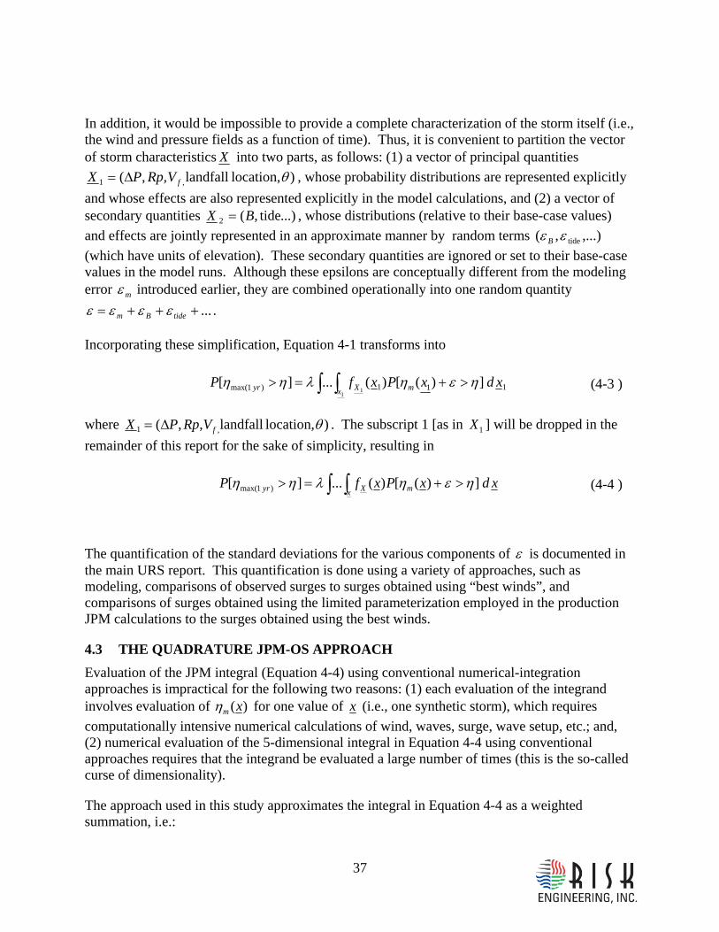
In addition, it would be impossible to provide a complete characterization of the storm itself (i.e., the wind and pressure fields as a function of time). Thus, it is convenient to partition the vector of storm characteristics X into two parts, as follows: (1) a vector of principal quantities

),locationlandfall,,( ,1 θfVRpPX Δ= , whose probability distributions are represented explicitly and whose effects are also represented explicitly in the model calculations, and (2) a vector of secondary quantities ...)tide,(2 BX = , whose distributions (relative to their base-case values) and effects are jointly represented in an approximate manner by random terms ,...),( tideεε B (which have units of elevation). These secondary quantities are ignored or set to their base-case values in the model runs. Although these epsilons are conceptually different from the modeling error mε introduced earlier, they are combined operationally into one random quantity

...+++= tideBm εεεε .

Incorporating these simplification, Equation 4-1 transforms into

∫∫ >+=>1

1 111)1max( ])([)(...][x mXyr xdxPxfP ηεηληη (4-3 )

where ),locationlandfall,,( ,1 θfVRpPX Δ= . The subscript 1 [as in 1X ] will be dropped in the remainder of this report for the sake of simplicity, resulting in

∫∫ >+=>x mXyr xdxPxfP ])([)(...][ )1max( ηεηληη (4-4 )

The quantification of the standard deviations for the various components of ε is documented in the main URS report. This quantification is done using a variety of approaches, such as modeling, comparisons of observed surges to surges obtained using “best winds”, and comparisons of surges obtained using the limited parameterization employed in the production JPM calculations to the surges obtained using the best winds.

4.3 THE QUADRATURE JPM-OS APPROACH Evaluation of the JPM integral (Equation 4-4) using conventional numerical-integration approaches is impractical for the following two reasons: (1) each evaluation of the integrand involves evaluation of )(xmη for one value of x (i.e., one synthetic storm), which requires computationally intensive numerical calculations of wind, waves, surge, wave setup, etc.; and, (2) numerical evaluation of the 5-dimensional integral in Equation 4-4 using conventional approaches requires that the integrand be evaluated a large number of times (this is the so-called curse of dimensionality).

The approach used in this study approximates the integral in Equation 4-4 as a weighted summation, i.e.:

38

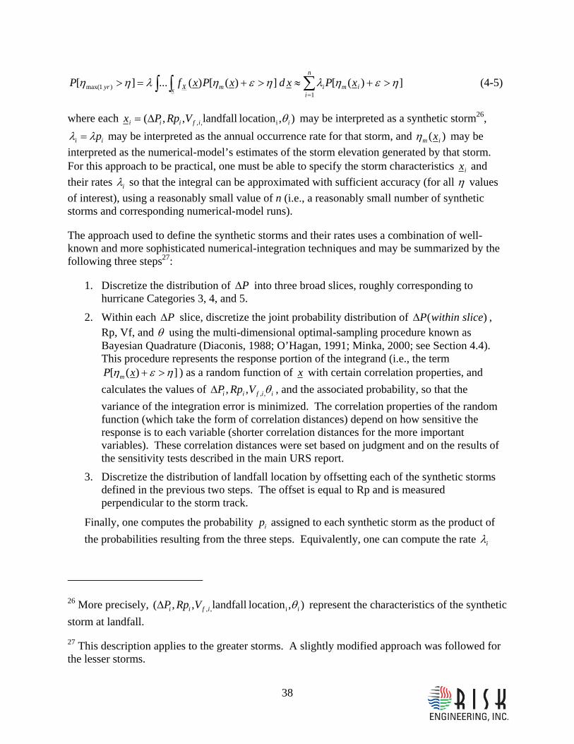
])([])([)(...][1

)1max( ∑∫∫=

>+≈>+=>n

iimix mXyr xPxdxPxfP ηεηληεηληη (4-5)

where each ),locationlandfall,,( i,, iifiii VRpPx θΔ= may be interpreted as a synthetic storm26,

ii pλλ = may be interpreted as the annual occurrence rate for that storm, and )( im xη may be interpreted as the numerical-model’s estimates of the storm elevation generated by that storm. For this approach to be practical, one must be able to specify the storm characteristics ix and their rates iλ so that the integral can be approximated with sufficient accuracy (for all η values of interest), using a reasonably small value of n (i.e., a reasonably small number of synthetic storms and corresponding numerical-model runs).

The approach used to define the synthetic storms and their rates uses a combination of well-known and more sophisticated numerical-integration techniques and may be summarized by the following three steps27:

1. Discretize the distribution of PΔ into three broad slices, roughly corresponding to hurricane Categories 3, 4, and 5.

2. Within each PΔ slice, discretize the joint probability distribution of )( slicewithinPΔ , Rp, Vf, and θ using the multi-dimensional optimal-sampling procedure known as Bayesian Quadrature (Diaconis, 1988; O’Hagan, 1991; Minka, 2000; see Section 4.4). This procedure represents the response portion of the integrand (i.e., the term

])([ ηεη >+xP m ) as a random function of x with certain correlation properties, and calculates the values of iifii VRpP θ,,,,Δ , and the associated probability, so that the variance of the integration error is minimized. The correlation properties of the random function (which take the form of correlation distances) depend on how sensitive the response is to each variable (shorter correlation distances for the more important variables). These correlation distances were set based on judgment and on the results of the sensitivity tests described in the main URS report.

3. Discretize the distribution of landfall location by offsetting each of the synthetic storms defined in the previous two steps. The offset is equal to Rp and is measured perpendicular to the storm track.

Finally, one computes the probability ip assigned to each synthetic storm as the product of the probabilities resulting from the three steps. Equivalently, one can compute the rate iλ

26 More precisely, ),locationlandfall,,( i,, iifii VRpP θΔ represent the characteristics of the synthetic storm at landfall.

27 This description applies to the greater storms. A slightly modified approach was followed for the lesser storms.

39

assigned to each synthetic storm as the product of the probabilities from the first two steps times the rate per unit length from Section 3 times the storm spacing.

4.4 BAYESIAN QUADRATURE APPROACH

4.4.1 Background The word Quadrature is often used to denote numerical techniques to approximate an integral of the form

∫= AdxxpxfI )()( ( 4-6 )

over some domain A, as a weighted sum of the form

)(

1i

n

ii xpwI ∑

=

≈ ( 4-7 )

where )(xf is typically a probability density function (i.e., it is positive and it integrates to unity) and )(xp represents a function belonging to a certain family of functions.

In our case, A represents a four-dimensional domain, )(xf represents the joint probability distribution of storm characteristics, and ])([)( ηεη >+= xPxp m represents the “surge effects” portion of the JPM integral (for many possible locations and for many possible values of η ).

The design of the quadrature involves specification of the number of nodes n, and selection of the node values ix and associated weights iw . These quantities depend on the functional form of )(xf and of the family of )(xp , and on the desired characteristics (e.g., accuracy) of the approximation. In our case, each node becomes one synthetic storm.

Classical (Gaussian) quadrature chooses the number of nodes, node values, and weights so that the summation will integrate the function exactly if )(xp is a polynomial of a certain degree and

)(xf is a particular function (e.g., a standard normal probability density). This technique is used frequently in one dimension (see Miller and Rice, 1983 for details and for results for a variety of probability distributions). Classical Quadrature is used in the main URS report for the reference-case or “JPM-Heavy (Gold Standard)” approach to represent the probability distribution of each individual storm characteristic. Extension of these zero-error rules to more than one dimension is problematic. The number of required nodes increases rapidly with the number of dimensions (see Minka, 2000). Furthermore, some of the weights often become negative (see Genz and Keister, 1996), which leads to less stable results and makes it impossible to interpret the weights as probabilities.

Bayesian quadrature, in contrast, considers a much broader probabilistically defined family of functions )(xp (namely, all possible realizations of a random function with a certain correlation structure), and chooses the node values and weights so that the integration error is minimized in a mean-squared sense. Conceptually, it is straightforward to extend Bayesian quadrature to

40

multiple dimensions, although it becomes computationally demanding for more than six or seven dimensions. According to Diaconis (1988), the approach dates back to the work of Poincare in 1896. It is also closely related to the technique known as Kriging (e.g., Journel and Huijbregts, 1978), and even to least-squares regression.

4.4.2 Derivation The derivation that follows for the Bayesian Quadrature approach borrows significantly from Minka (2000), although we have modified some of the notation, and we add a constraint on the sum of the weights (which we borrow from Kriging). The random-function theory and random-vector algebra used in this section may be unfamiliar to many readers. Readers may choose to skip this section, and rely on the more qualitative description provided above.

We begin by idealizing the function )(xp in Equation 4-4 as a random function in m-dimensional space with mean zero and with autocovariance function )]()([),( ypxpEyxk = 28 29 30, where ][⋅E denotes mathematical expectation (i.e., ][zE the average value of quantity z over all possible realizations of )(xp ), and x and y are any two arbitrary values of x. The autocovariance function contains information about the degree of continuity of realizations of

)(xp , at both small and large scales (e.g., Vanmarcke, 1983).

Let ],...,,[ 21 nxxxD = denote n nodes31 for which )(xp has been evaluated, so that we know the values of )](),...,(),([)( 21 nxpxpxpDp = . Because we know the value of )(xp at these n points and )(xp has some correlation structure, we also have some information about the value of )(xp at other x values (particularly at x values in the vicinity of a node where the function has been sampled). This situation is illustrated in Figure 4-1.

28 m is the number of dimensions for the integral in Equation 4-6. In this derivation, x and y are m-dimensional vectors, but we will not use underline or boldface for them for the sake of simplicity

29 Details on the functional form of ),( yxk will be considered in the next sub-section. The only requirement at this stage is that the required integrals involving ),( yxk and )(xf do not diverge.

30 Minka (2000) assumes that )(xp is a Gaussian random process (or random field, if the number of dimensions is greater than two). Actually, the Gaussian assumption is not required, because all the results needed may be obtained using first and second moments, for which the following two assumptions are sufficient: (1) )](|)([ DpxpE is a linear function of )(Dp , and (2)

)](|)([ DpxpVar does not dependent on )(Dp .

31 In our m-dimensional integration space, each node location ix denotes m nodal coordinates.

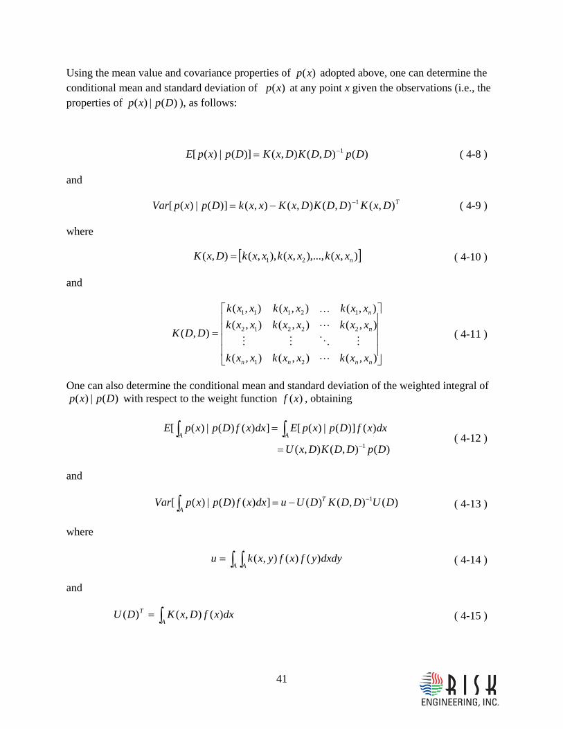
41

Using the mean value and covariance properties of )(xp adopted above, one can determine the conditional mean and standard deviation of )(xp at any point x given the observations (i.e., the properties of )(|)( Dpxp ), as follows:

)(),(),()](|)([ 1 DpDDKDxKDpxpE −= ( 4-8 )

and

TDxKDDKDxKxxkDpxpVar ),(),(),(),()](|)([ 1−−= ( 4-9 )

where

[ ]),(),...,,(),,(),( 21 nxxkxxkxxkDxK = ( 4-10 )

and

⎥⎥⎥⎥

⎦

⎤

⎢⎢⎢⎢

⎣

⎡

=

),(),(),(

),(),(),(),(),(),(

),(

21

22212

12111

nnnn

n

n

xxkxxkxxk

xxkxxkxxkxxkxxkxxk

DDK

L

MOMM

L

K

( 4-11 )

One can also determine the conditional mean and standard deviation of the weighted integral of )(|)( Dpxp with respect to the weight function )(xf , obtaining

)(),(),(

)(])(|)([])()(|)([1 DpDDKDxU

dxxfDpxpEdxxfDpxpEAA

−=

= ∫∫ ( 4-12 )

and

)(),()(])()(|)([ 1 DUDDKDUudxxfDpxpVar T

A

−−=∫ ( 4-13 )

where

∫ ∫=A A

dxdyyfxfyxku )()(),( ( 4-14 )

and

∫= A

T dxxfDxKDU )(),()( ( 4-15 )

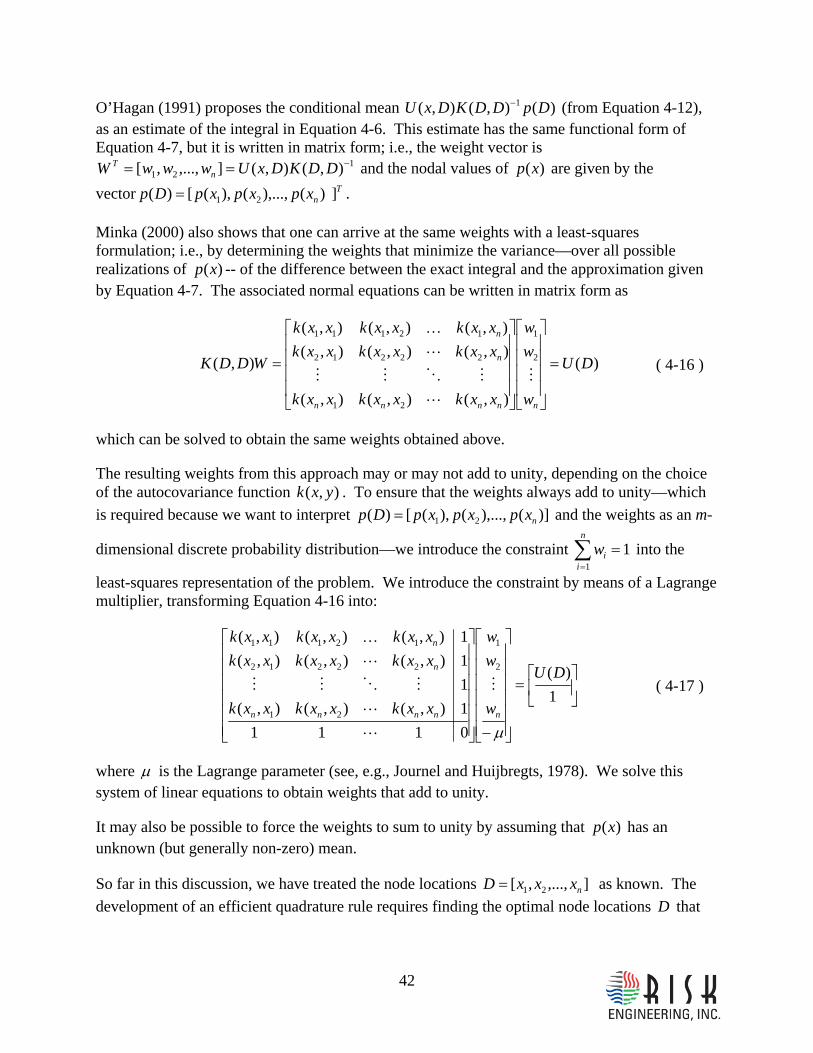
42

O’Hagan (1991) proposes the conditional mean )(),(),( 1 DpDDKDxU − (from Equation 4-12), as an estimate of the integral in Equation 4-6. This estimate has the same functional form of Equation 4-7, but it is written in matrix form; i.e., the weight vector is

121 ),(),(],...,,[ −== DDKDxUwwwW n

T and the nodal values of )(xp are given by the vector T

nxpxpxpDp ])(),...,(),([)( 21= .

Minka (2000) also shows that one can arrive at the same weights with a least-squares formulation; i.e., by determining the weights that minimize the variance—over all possible realizations of )(xp -- of the difference between the exact integral and the approximation given by Equation 4-7. The associated normal equations can be written in matrix form as

)(

),(),(),(

),(),(),(),(),(),(

),( 2

1

21

22212

12111

DU

w

ww

xxkxxkxxk

xxkxxkxxkxxkxxkxxk

WDDK

nnnnn

n

n

=

⎥⎥⎥⎥

⎦

⎤

⎢⎢⎢⎢

⎣

⎡

⎥⎥⎥⎥

⎦

⎤

⎢⎢⎢⎢

⎣

⎡

=M

L

MOMM

L

K

( 4-16 )

which can be solved to obtain the same weights obtained above.

The resulting weights from this approach may or may not add to unity, depending on the choice of the autocovariance function ),( yxk . To ensure that the weights always add to unity—which is required because we want to interpret )](),...,(),([)( 21 nxpxpxpDp = and the weights as an m-

dimensional discrete probability distribution—we introduce the constraint 11

=∑=

n

iiw into the

least-squares representation of the problem. We introduce the constraint by means of a Lagrange multiplier, transforming Equation 4-16 into:

⎥⎦

⎤⎢⎣

⎡=

⎥⎥⎥⎥⎥⎥

⎦

⎤

⎢⎢⎢⎢⎢⎢

⎣

⎡

−⎥⎥⎥⎥⎥⎥

⎦

⎤

⎢⎢⎢⎢⎢⎢

⎣

⎡

1)(

01111),(),(),(11),(),(),(1),(),(),(

2

1

21

22212

12111

DU

w

ww

xxkxxkxxk

xxkxxkxxkxxkxxkxxk

nnnnn

n

n

μ

M

L

L

MOMM

L

K

( 4-17 )

where μ is the Lagrange parameter (see, e.g., Journel and Huijbregts, 1978). We solve this system of linear equations to obtain weights that add to unity.

It may also be possible to force the weights to sum to unity by assuming that )(xp has an unknown (but generally non-zero) mean.

So far in this discussion, we have treated the node locations ],...,,[ 21 nxxxD = as known. The development of an efficient quadrature rule requires finding the optimal node locations D that

43

minimizes the variance in Equation 4-13 32, for a pre-specified value of n. Note that each ix in D represents the coordinates of a node in m-dimensional space. Thus, determination of the optimal D is an ( nm× )-dimensional optimization problem. We provide details on the algorithm used in Section 4.5.4

We have not shown that all the weights are non-negative, and in fact negative weights do arise when the nodal vector ],...,,[ 21 nxxxD = is specified arbitrarily (i.e., without optimization)33. On the other hand, it is reasonable to expect (and one may be able to prove) that optimization of

],...,,[ 21 nxxxD = so as to minimize the variance in Equation 4-13, forces all the weights to be positive. This argument is related to the concept of quadrature stability (i.e., the sum of the absolute values of the weights) employed by Genz and Keister (1996). In our practical applications, the approach introduced here has always led to positive weights when D is optimized. Negative weights, if they happen to arise, may be eliminated by employing a numerical optimization scheme with inequality constraints on the weights.

4.5 IMPLEMENTATION OF BAYESIAN QUADRATURE FOR JPM-OS This sub-section provides a number of details on how Bayesian Quadrature procedure is implemented as part of the Quadrature JPM-OS formulation used in this study. These details were left out of the derivation above, for the sake of generality and simplicity.

4.5.1 Probability distribution: choice for )(xf

The Quadrature JPM-OS formulation must be flexible enough to accommodate the probability distributions employed in Section 3. On the other hand, implementation of the Bayesian Quadrature formulation described above using a general form for )(xf would require the repeated evaluation of the integrals in Equations 4-14 and 4-15, which are likely more complex than the JPM integrals we are trying to solve in the first place.

Instead, we formulate the problem in m-dimensional standard normal-distribution space, determine the coordinates of the integration nodes in that space, and then convert these nodal

32 Note that now we have two nested optimizations, both of which seek to minimize the variance of the integration error. At the inner level of nesting, there is the optimization to determine the best weights (for given nodal locations D). This is done analytically, obtaining the weights given by the solution of Equation 4-17. At the outer level, there is the search for the set of nodal values D that minimize the variance given by Equaion 4-13 . This is done numerically (more details on the optimization algorithm will be provided in the next section).

33 Consider the case where two nodes (call them nodes j and 'j ) have identical coordinates. In this case, their weights can take any pair of values that satisfy the condition jjj www =+ ' (one

of which can be made negative), where j

w is the weight that one would obtain for node j if

node 'j were removed.

44

coordinates to the “physical” space of ,, pRPΔ etc., in a manner that takes into account their joint probability distribution.

This transformation of each nodal value from normal space (represented by T

mXXXX ],,,[ 21 L= ) to “physical” space (represented by TmZZZZ ],,,[ 21 L= ) 34 consists of

two steps. First, we write the joint cumulative distribution of the physical quantities as a product of conditional cumulative distributions, i.e.,

12121312121 |,|| −

×××=mmm ZZZZZZZZZZZZZ FFFFF LL L ( 4-18 )

Then, we sequentially transform each normally distributed jX into the corresponding physical quantity jZ , using their corresponding conditional cumulative distributions to ensure that jZ has the proper conditional distribution, i.e.,

)]([1| 11 jZZZj XFZ

jjΦ= −

−L ( 4-19 )

where )(⋅Φ represents the standard normal cumulative distribution function and ][1| 11

⋅−

−jj ZZZF L

represents the inverse of the cumulative distribution function of jZ given 121 ..., −jZZZ . This transformation is performed only once for each sampling node, after the optimization in normal space has been completed.

This approach for the transformation of multivariate probability distributions is the so-called Rosenblatt transformation (see Madsen et al., 1986). It is commonly used in structural reliability theory and is built into structural reliability software (e.g., Gollwitzer et al., 2006; Risk Engineering, 1996). The approach allows the practical implementation of Bayesian Quadrature for virtually any choice of joint probability distributions, as required for JPM-OS.

One can also achieve the distribution transformations by altering the weights, or by using a combination of both approaches. This is not done in this study.

4.5.2 Correlation Structure of )(xp : the choice for ),( yxk and the specification of correlation distances

We use the correlation structure of )(xp , as represented by the covariance function ),( yxk , to specify the importance of the corresponding physical quantity in the surge calculations. If the

34 In this section and the section that follows, the subscripts denote the coordinates of one point in m-dimensional space (j=1,…m). This is different from Section 4.4.2, where the subscripts denote different sampling nodes (i=1,…,n) in m-dimensional space.

45

physical quantity corresponding to the j-th component of x is important, correlation decays faster in that direction than in the direction corresponding to a less important quantity.

One of the consequences of formulating and solving the Bayesian Quadrature problem in normal space is that we must also define ),( yxk in normal space. Also, we must choose a functional form that facilitates analytical evaluation of the integrals in Equations 4-14 and 4-15.

We choose the double-exponential functional form for the covariance function, i.e.,

∏= ⎥

⎥

⎦

⎤

⎢⎢

⎣

⎡

⎟⎟⎠

⎞⎜⎜⎝

⎛ −−==

m

j j

jj

cyx

ypxpEyxk1

2

2 exp)]()([),( σ ( 4-20 )

where jc controls how quickly the correlation decays in the direction of a particular component 35 36 37. jc is related to the corresponding correlation distance or scale of fluctuation jd

(Vanmarcke, 1983) by the relation jj cd π= . Because the algorithm operates in standard normal space, jc and jd have no physical units.

One of the critical steps in the Quadrature JPM-OS analysis is the specification of the correlation distances jd associated with the various hurricane characteristics. This is made more difficult because these correlation distances are specified in normal space, not in physical space. The following discussion provides some guidance to facilitate this step.

In a relative sense, the Quadrature JPM-OS algorithm tends to spread the sampling nodes more faithfully along those directions for which )(xp has lower correlation distances, providing a closer match to the marginal probability distributions in those directions. Thus, it is important to specify correlation distances that relate to the importance of the various physical quantities, in order to obtain an optimal allocation of effort among the various directions.

In an absolute sense, numerical experiments in one dimension show that low values of the correlation distance cause the algorithm to be more cautious and tend towards equal weights, while high values provide a wide range of weights, approaching those obtained by Gaussian quadrature. The ideal choice is somewhere in between.

35 In this section, the subscripts denote the coordinates of one point in m-dimensional space (j=1,…m); x and y denote two points in that m-dimensional space.

36 This correlation model implies that the random field is homogeneous and twice differentiable (in a second-order sense).

37 The variance 2σ cancels out in the results of section 4.4.2 and will be omitted in the material that follows.

46

The following values provide preliminary guidance for the choice of correlation distances:

• Sensitive (important): jd =1 to 3

• Insensitive (unimportant): jd = 4 to 6

4.5.3 Evaluation of Required Integrals

The choice of a normal distribution for )(xf and a double-exponential correlation function (Equation 4-20) make it possible to evaluate the required integrals analytically; this provides significant computational advantages for the optimization of the node locations. The integral required for Equation 4-14 takes the form

∏∫ ∫=

−

⎥⎥⎦

⎤

⎢⎢⎣

⎡+==

m

j jA A c

dxdyyfxfyxku1

2/1

2

41)()(),( ( 4-21 )

where jc is the scaling parameter in Equation 4-20.

The integral required for the i-th element of the vector TDU )( in Equation 4-15 is given by

∏∫=

−

⎪⎭

⎪⎬⎫

⎪⎩

⎪⎨⎧

⎥⎥⎦

⎤

⎢⎢⎣

⎡

+−

⎥⎥⎦

⎤

⎢⎢⎣

⎡+=

m

j j

ji

jA i c

x

cdxxfxxk

12

2,

2/1

2 2exp21)(),( ( 4-22 )

where ix is the vector with the coordinates of the i-th node and jix , is its component in the j-th direction.

4.5.4 Optimization Algorithm As was indicated earlier, determination of n optimal sampling points in m dimensions constitutes an ( nm× )-dimensional optimization problem. We perform this optimization using an algorithm developed by Powell (2004), which does not require derivatives. Convergence is fast for the number of dimensions and nodes used in this study.

4.5.5 Closing Remarks Because we make a number of assumptions regarding the functional form and parameters of the autocovariance function ),( yxk of ])([)( ηεη >+= xPxp m , it is important to validate the Quadrature JPM-OS scheme (i.e., the number of nodes and the correlation distances).

In this study, we validate the JPM-OS scheme for the larger storms by comparing the cumulative distributions of surge obtained using the JPM-OS scheme and a reference case JPM scheme (denoted JPM-Heavy (Gold Standard)), using the SLOSH software to compute the surge in both schemes. These comparisons are documented in the main URS report.

One can also perform this validation using a parametric surge model (e.g., Irish et al., 2007).

47

4.6 APPLICATION OF THE QUADRATURE JPM-OS APPROACH This section documents the application of the Quadrature JPM-OS approach to hurricanes affecting the Mississippi coast. We present separate results for the greater and lesser storms.

4.6.1 JPM-OS Scheme for Greater Storms The following is a description of the JPM-OS 6 scheme, which is the scheme adopted for the final calculations, after experimenting with a number of other schemes having different numbers of nodes and correlation distances. This scheme incorporate the rates and probability distributions for the greater storms, as developed in Section 3. Table 4-1 shows the various slices of the PΔ distribution, their probabilities, and the number of nodes used in the Bayesian-Quadrature discretization for each slice. Table 4-2 shows the correlation distances used in the Bayesian-Quadrature procedure. These values were chosen based on the extensive sensitivity results presented in the main URS report, and then refined so that they preserve the marginal moments of the most important quantities.

Figure 4-2 provides an illustration of the resulting synthetic storms (for one landfall location; i.e., prior to the distance-offsetting step in Section 4.3). Each chart on the main diagonal shows the probability distribution of the corresponding quantity (in the form of a histogram), as represented in the JPM-OS 6 discretization. Each off-diagonal scatter diagram shows how each pair of quantities (e.g., PΔ and Rp) are jointly distributed in the JPM-OS 6 scheme, with the areas of the circles being proportional to the associated annual rates. Table 4-3 lists the corresponding parameter values, probabilities, and rates.

As indicated earlier, we validate the JPM-OS 6 scheme by comparing the cumulative distributions of surge obtained using the JPM-OS scheme and a reference-case JPM scheme (denoted JPM-Heavy (Gold Standard)), using the SLOSH software to compute the surge in both schemes. These comparisons were performed for a large number of locations and are documented in the main URS report. This validation was performed prior to integration over ε . The match would have been even closer if the comparison had been performed after integration over ε because this step makes )(xp smoother.

4.6.2 JPM-OS Scheme for Lesser Storms We followed a simpler approach for the lesser storms ( PΔ =31 to 48 mb). In particular, we did not divide the distribution of PΔ into slices because these storms span a narrower range of PΔ and because the associated probability distribution is less skewed. The number of nodes employed is 13. Table 4-4 lists the correlation distances used.

We initially developed the JPM-OS scheme using the PRp Δ| distribution shown in Figure 3-7. The resulting parameter values were then used to generate the synthetic storms and perform the wind, wave, and surge calculations. Later in the project, we changed the PRp Δ| for the lesser storms to that in Figure 3-10. We were able to adjust the weights to reflect the new distribution, without a significant loss of accuracy in the JPM-OS scheme. Table 4-5 lists the corresponding parameter values, probabilities, and rates.

48

We also validated this JPM-OS scheme (with the adjusted weights). The validation approach was simpler than that used for the greater storms. It used a parametric surge model somewhat simpler than the model of Irish et al. (2008) instead of SLOSH, it considered only one location and one storm track, and it used a 36-node JPM-OS scheme as the standard for comparison. Results are shown in Figure 4-3. Checks on statistical moments were also performed.

4.7 GENERATION OF SYNTHETIC STORMS The numerical wind and wave calculations require as inputs the entire history of the synthetic storm, since the moment in enters the Gulf. This history consists of hourly values of the coordinates of the storm center, PΔ (or central pressure) , Rp, and forward velocity. We generate this sequence of values from the storm parameters associated with each Quadrature JPM-OS node, as described below. All the storms generated here make landfall at the Coastal Reference Point defined in Section 3. OWI then offsets these storms laterally, as discussed earlier.

The approach we use to generate the storm tracks--given coastfVP ),,( θΔ and )(offshorepR -- is a purely deterministic approach and is largely based on the approach developed by USACE in their probabilistic surge studies for Mississippi and Louisiana (Resio, 2007), and is described below.

• The geometry of the tracks is similar to the USACE tracks (Figures 12-14 in Resio, 2007), although we use a different algorithm to generate the track geometries. Also, our algorithm can generate tracks with any arbitrary heading between -90 and 90 degrees, instead of being restricted to three possible headings.

• Storms with )(offshorepR > 10 nmi vary in intensity, radius, and Holland B linearly over the last 90 nm prior to landfall, according to the following rules:

• Rp (landfall) = 1.3*Rp (offshore)

• B (offshore) = 1.27

• B (landfall) = 1.0

• B (3 hrs after landfall) = 0.9

• Decrease in PΔ ( mb) = Rp (offshore, nmi) - 6 (maximum increase is 18 mb, minimum is 5 mb)

• Storms with )(offshorepR < 10 nmi do not undergo any weakening or other changes prior to landfall.

• After landfall, linear variation continues for 2 hours, with the same slopes they had prior to landfall. Weakening of PΔ continues after this point, following the exponential-decay model of Vickery and Twisdale (1995).

Figure 4-4 and Figure 4-5 show the tracks for the greater and lesser synthetic storms, respectively. Tracks that make landfall with a NNW heading are similar in appearance to the RICK-fan tracks in Figure 12 of Resio (2007). More oblique tracks are similar to the + 45-degree tracks of Resio (2007). All these storms make landfall at the Coastal Reference Point. We will refer to them as the master or reference tracks. OceanWeather then offset each of these

49

master synthetic storms by pR , creating multiple offset synthetic tracks that cover the entire Mississippi coast. The latter synthetic storms are the ones actually used for the numerical wind, wave, and surge calculations.

Figure 4-6 shows the track and the variation in time of the key storm parameters for one master synthetic storm. This figure, and similar figures for all other synthetic storms, was generated by OceanWeather

The top panel of Figure 4-6 shows the track of the storm we generate here (in color; the master track), as well as the offset tracks generated by OceanWeather. The offset tracks have a spacing of Rp and a uniformly-distributed random offset from the master track.

The three bottom panels of Figure 4-6 show the variation in time of the key storm parameters for the master track. The time of landfall is represented by a short vertical stroke.

4.8 SUMMARY This section documents the development of a set of synthetic storms, and associated annual rates, based on the probabilistic hurricane model developed in Section 3. These storms, and their rates, are representative of future hurricanes that may generate significant storm surge to the inhabitants and infrastructure along the Mississippi coast.

The section also describes the Quadrature JPM-OS methodology employed to generate these synthetic storms, and provides details on the application of this methodology. Results from validation calculations confirm that the accuracy of the Quadrature JPM-OS scheme employed.

The synthetic storms generated here were used by OceanWeather to generate a complete set of synthetic storms, by offsetting them so that they cover the entire Mississippi coast and portions of adjacent states. These storms were then used by URS and other URS contractors to calculate the wind, waves, and surge generated by each storm at a number of grid points, and these were used to compute surge-exceedence statistics. These steps are documented in the main URS report.

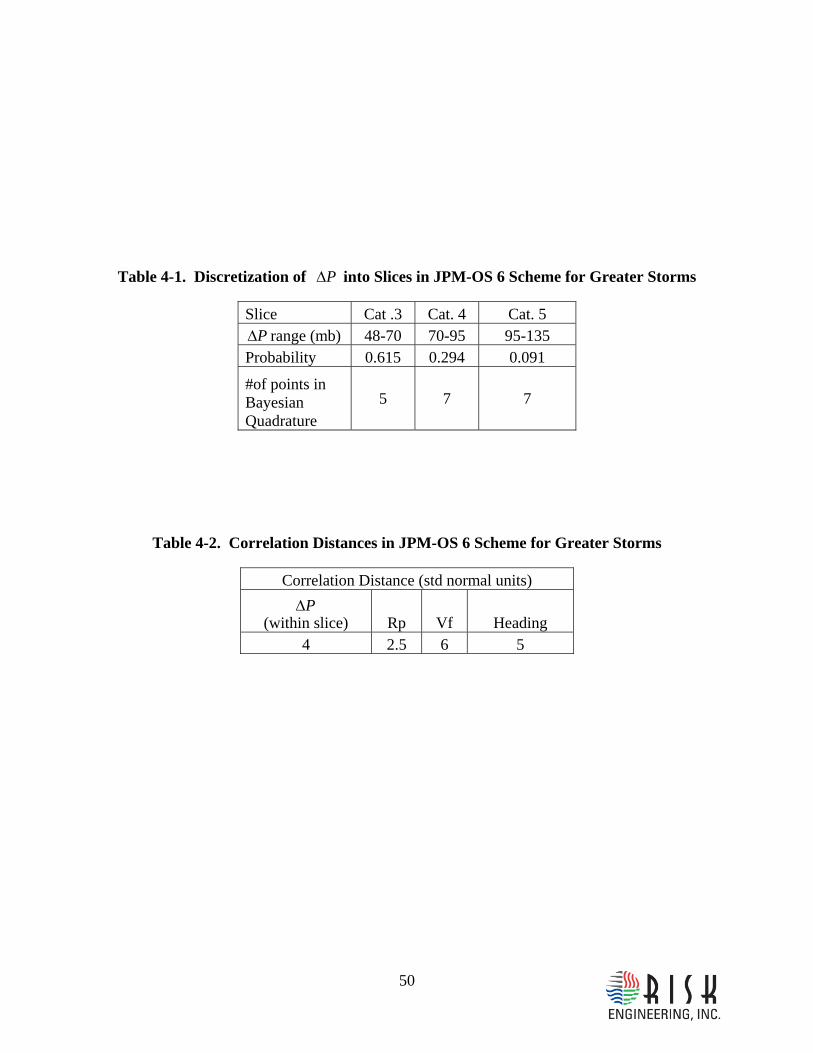
50

Table 4-1. Discretization of PΔ into Slices in JPM-OS 6 Scheme for Greater Storms

Slice Cat .3 Cat. 4 Cat. 5 PΔ range (mb) 48-70 70-95 95-135

Probability 0.615 0.294 0.091

#of points in Bayesian Quadrature

5 7 7

Table 4-2. Correlation Distances in JPM-OS 6 Scheme for Greater Storms

Correlation Distance (std normal units) PΔ

(within slice) Rp Vf Heading 4 2.5 6 5

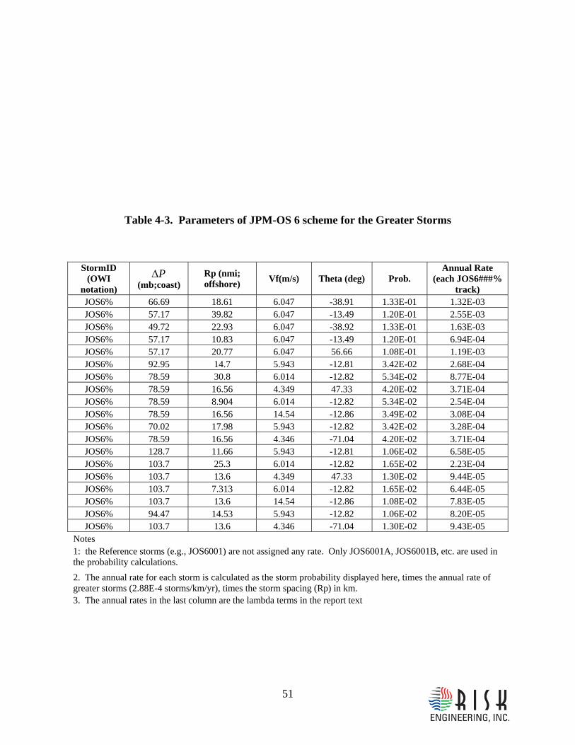
51

Table 4-3. Parameters of JPM-OS 6 scheme for the Greater Storms

StormID (OWI

notation) PΔ

(mb;coast) Rp (nmi; offshore) Vf(m/s) Theta (deg) Prob.

Annual Rate (each JOS6###%

track) JOS6% 66.69 18.61 6.047 -38.91 1.33E-01 1.32E-03 JOS6% 57.17 39.82 6.047 -13.49 1.20E-01 2.55E-03 JOS6% 49.72 22.93 6.047 -38.92 1.33E-01 1.63E-03 JOS6% 57.17 10.83 6.047 -13.49 1.20E-01 6.94E-04 JOS6% 57.17 20.77 6.047 56.66 1.08E-01 1.19E-03 JOS6% 92.95 14.7 5.943 -12.81 3.42E-02 2.68E-04 JOS6% 78.59 30.8 6.014 -12.82 5.34E-02 8.77E-04 JOS6% 78.59 16.56 4.349 47.33 4.20E-02 3.71E-04 JOS6% 78.59 8.904 6.014 -12.82 5.34E-02 2.54E-04 JOS6% 78.59 16.56 14.54 -12.86 3.49E-02 3.08E-04 JOS6% 70.02 17.98 5.943 -12.82 3.42E-02 3.28E-04 JOS6% 78.59 16.56 4.346 -71.04 4.20E-02 3.71E-04 JOS6% 128.7 11.66 5.943 -12.81 1.06E-02 6.58E-05 JOS6% 103.7 25.3 6.014 -12.82 1.65E-02 2.23E-04 JOS6% 103.7 13.6 4.349 47.33 1.30E-02 9.44E-05 JOS6% 103.7 7.313 6.014 -12.82 1.65E-02 6.44E-05 JOS6% 103.7 13.6 14.54 -12.86 1.08E-02 7.83E-05 JOS6% 94.47 14.53 5.943 -12.82 1.06E-02 8.20E-05 JOS6% 103.7 13.6 4.346 -71.04 1.30E-02 9.43E-05

Notes 1: the Reference storms (e.g., JOS6001) are not assigned any rate. Only JOS6001A, JOS6001B, etc. are used in the probability calculations. 2. The annual rate for each storm is calculated as the storm probability displayed here, times the annual rate of greater storms (2.88E-4 storms/km/yr), times the storm spacing (Rp) in km. 3. The annual rates in the last column are the lambda terms in the report text

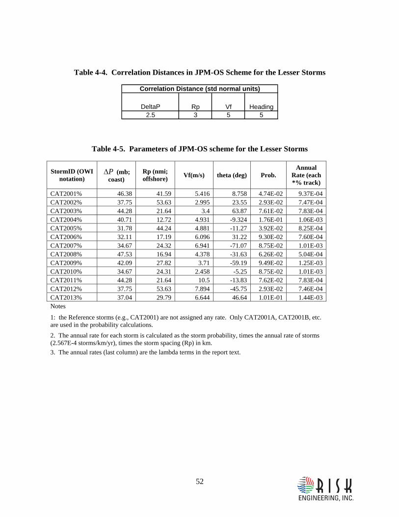
52

Table 4-4. Correlation Distances in JPM-OS Scheme for the Lesser Storms

DeltaP Rp Vf Heading2.5 3 5 5

Correlation Distance (std normal units)

Table 4-5. Parameters of JPM-OS scheme for the Lesser Storms

StormID (OWI notation)

PΔ (mb; coast)

Rp (nmi; offshore) Vf(m/s) theta (deg) Prob.

Annual Rate (each *% track)

CAT2001% 46.38 41.59 5.416 8.758 4.74E-02 9.37E-04 CAT2002% 37.75 53.63 2.995 23.55 2.93E-02 7.47E-04 CAT2003% 44.28 21.64 3.4 63.87 7.61E-02 7.83E-04 CAT2004% 40.71 12.72 4.931 -9.324 1.76E-01 1.06E-03 CAT2005% 31.78 44.24 4.881 -11.27 3.92E-02 8.25E-04 CAT2006% 32.11 17.19 6.096 31.22 9.30E-02 7.60E-04 CAT2007% 34.67 24.32 6.941 -71.07 8.75E-02 1.01E-03 CAT2008% 47.53 16.94 4.378 -31.63 6.26E-02 5.04E-04 CAT2009% 42.09 27.82 3.71 -59.19 9.49E-02 1.25E-03 CAT2010% 34.67 24.31 2.458 -5.25 8.75E-02 1.01E-03 CAT2011% 44.28 21.64 10.5 -13.83 7.62E-02 7.83E-04 CAT2012% 37.75 53.63 7.894 -45.75 2.93E-02 7.46E-04 CAT2013% 37.04 29.79 6.644 46.64 1.01E-01 1.44E-03 Notes

1: the Reference storms (e.g., CAT2001) are not assigned any rate. Only CAT2001A, CAT2001B, etc. are used in the probability calculations. 2. The annual rate for each storm is calculated as the storm probability, times the annual rate of storms (2.567E-4 storms/km/yr), times the storm spacing (Rp) in km. 3. The annual rates (last column) are the lambda terms in the report text.

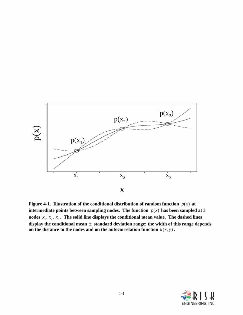
53

x1 x2 x3

p(x1)

p(x2)p(x3)

p(x)

x

Figure 4-1. Illustration of the conditional distribution of random function )(xp at intermediate points between sampling nodes. The function )(xp has been sampled at 3 nodes 321 ,, xxx . The solid line displays the conditional mean value. The dashed lines display the conditional mean ± standard deviation range; the width of this range depends on the distance to the nodes and on the autocorrelation function ),( yxk .

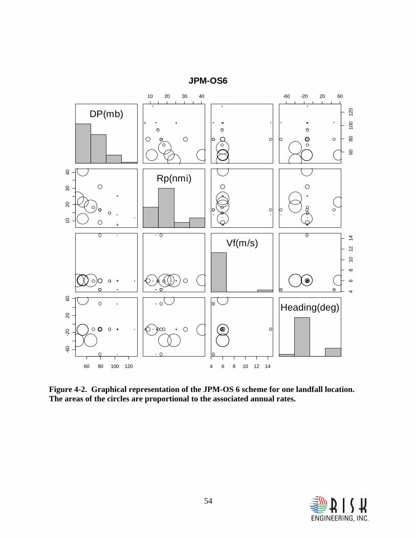
54

DP(mb)

10 20 30 40 -60 -20 20 60

6080

100

120

1020

3040

Rp(nmi)

Vf(m/s)

46

810

1214

60 80 100 120

-60

-20

2060

4 6 8 10 12 14

Heading(deg)

JPM-OS6

Figure 4-2. Graphical representation of the JPM-OS 6 scheme for one landfall location. The areas of the circles are proportional to the associated annual rates.

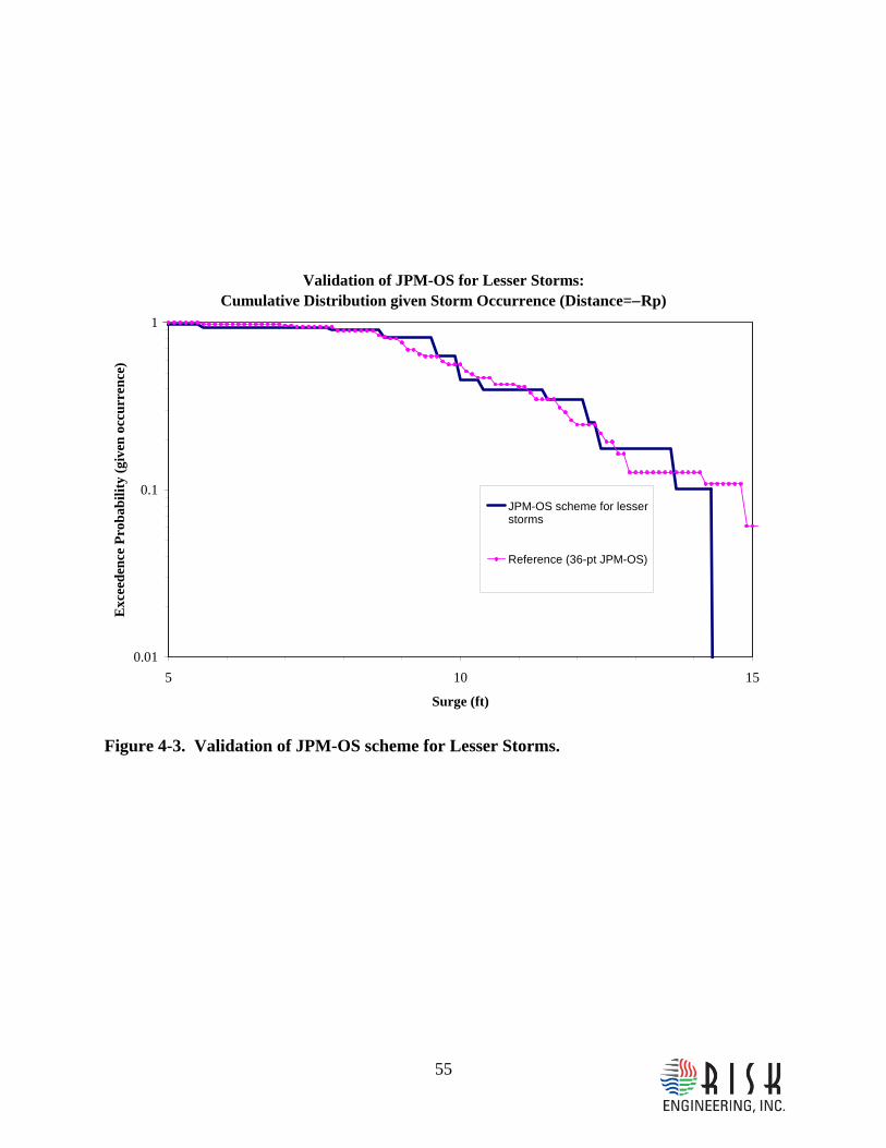
55

Validation of JPM-OS for Lesser Storms:Cumulative Distribution given Storm Occurrence (Distance=−Rp)

0.01

0.1

1

5 10 15

Surge (ft)

Exc

eede

nce

Prob

abili

ty (g

iven

occ

urre

nce)

JPM-OS scheme for lesserstorms

Reference (36-pt JPM-OS)

Figure 4-3. Validation of JPM-OS scheme for Lesser Storms.

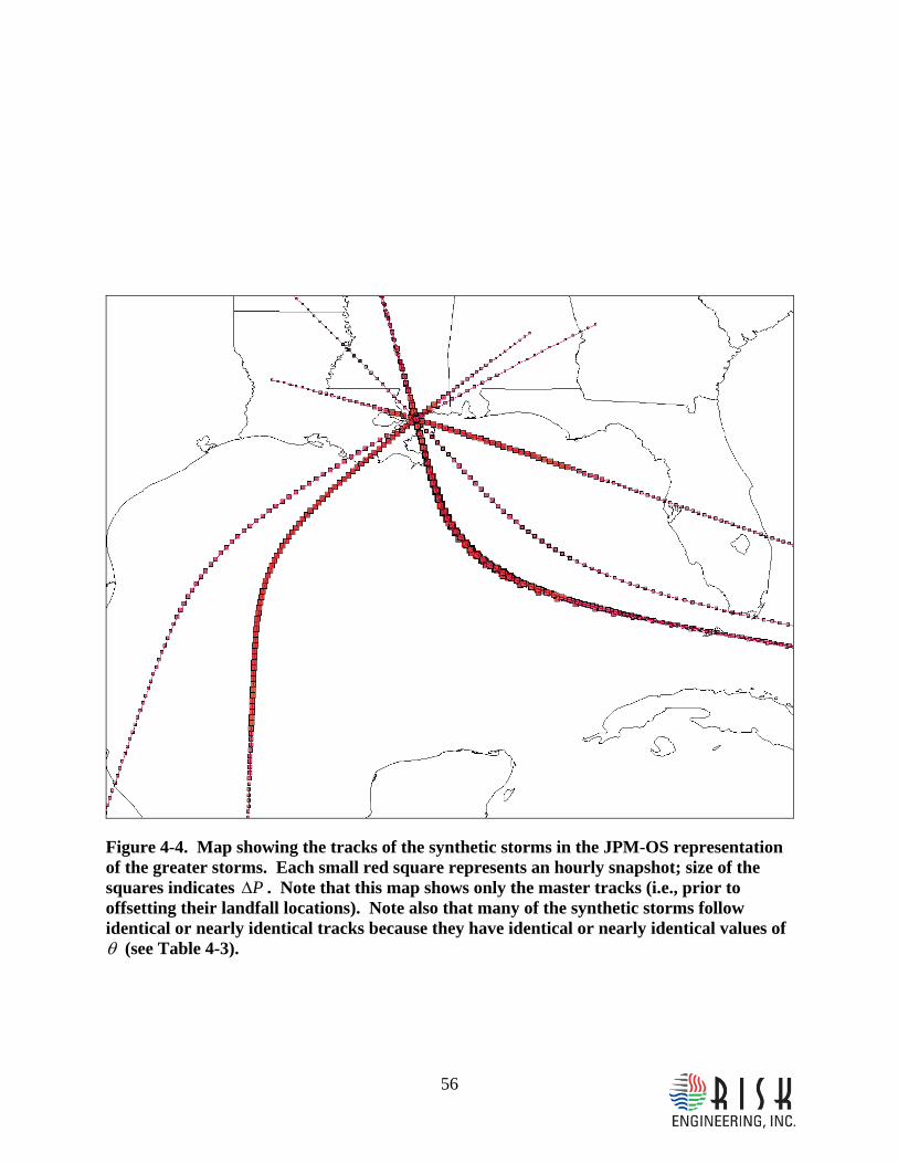
56

Figure 4-4. Map showing the tracks of the synthetic storms in the JPM-OS representation of the greater storms. Each small red square represents an hourly snapshot; size of the squares indicates PΔ . Note that this map shows only the master tracks (i.e., prior to offsetting their landfall locations). Note also that many of the synthetic storms follow identical or nearly identical tracks because they have identical or nearly identical values of θ (see Table 4-3).

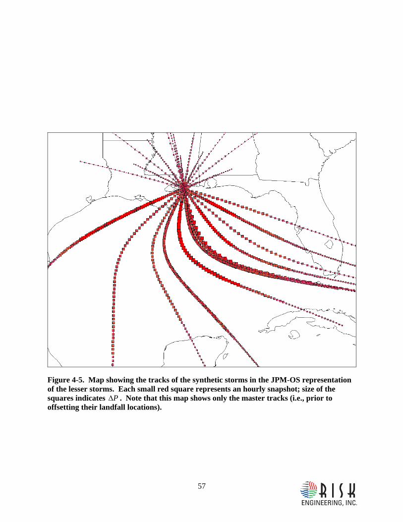
57

Figure 4-5. Map showing the tracks of the synthetic storms in the JPM-OS representation of the lesser storms. Each small red square represents an hourly snapshot; size of the squares indicates PΔ . Note that this map shows only the master tracks (i.e., prior to offsetting their landfall locations).

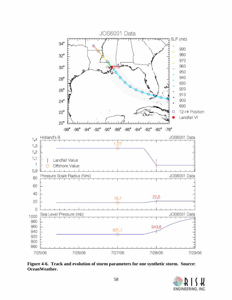
58

Figure 4-6. Track and evolution of storm parameters for one synthetic storm. Source: OceanWeather.

59

5 QUALITY CONTROL AND ASSURANCE

The work presented here was subject to extensive Peer Review during the JPM Group meeting of October 31, 2006 (Boston), and the Senior Review Team meetings of January 30 and31, 2007 (Tallahassee) and May 8 and 9, 2007 (Tallahassee). In addition, extensive comparisons have been performed between the JPM model parameters developed by Risk Engineering and the Corps of Engineers MSCIP Study. Section 3.5 of this report contains comparisons for the most important model parameters, namely PΔ exceedence rates, and distribution of PRp Δ| . Furthermore, Section 5.4 of URS (2008) contains comparisons in terms of 100-year surges.

The Risk Engineering principal investigator also reviewed his calculations and results more than once, performed internal consistency checks (e.g., checks of distribution moments), and compared results to those obtained by him in proprietary studies for the Gulf of Mexico.

60

6 REFERENCES

Bell, G. D., and M. Chelliah (2006). Leading tropical modes associated with interannual and multi-decadal fluctuations in North Atlantic hurricane activity. J. Climate. 19, 590-612.

Benjamin, J.R. and Cornell, C.A. 1970. Probability, Statistics, and Decision for Civil Engineers. New York, New York: McGraw-Hill.

Chouinard, L. E. (1992), “A Statistical Method for Regional Design Wave Heights in the Gulf of Mexico,” OTC 6832, Proceedings of the Offshore Technology Conference, Houston, TX.

Chouinard, L.M., and C. Liu (1997). “Model for Recurrence Rate of Hurricanes in Gulf of Mexico,” Journal of Waterway, Port, Coastal and Ocean Engineering, Vol. 123, No. 3, pp. 113-119.

Chouinard, L.M., C. Liu, and C. K. Cooper (1997). “Model for Severity Rate of Hurricanes in Gulf of Mexico,” Journal of Waterway, Port, Coastal and Ocean Engineering, Vol. 123, No. 3, pp. 120-129.

Cooper, C., and J. Stear (2006). Hurricane Climate in the Gulf of Mexico. Offshore Technology Conference, OTC 18418.

Diaconis, P. (1988). Bayesian numerical analysis. Statistical Decision Theory and Related Topics IV (pp. 163--175).

Efron, B. (1982). The Jacknife, the Bootstrap, and other Resampling Plans. Society for Industrial and Applied Mathematics, Philadelphia.

Genz, A., and B. Keister (1996). Fully Symmetric Interpolatory Rules for Multiple Integrals over Infinite Regions with Gaussian Weight. J. Comp. Appl. Math. 71 (1996), pp. 299-309

Gollwitzer, S., B. Kirchgaßner, R. Fischer, and R. Rackwitz (2006). PERMAS-RA/STRUREL system of programs for probabilistic reliability analysis. Structural Safety 28 (2006) 108–129.

Gray, W.M., (1984) Atlantic seasonal hurricane frequency. Part II: Forecasting its variability, Mon. Wea. Rev., 112, 1649-1668.

Gualdi, S., E. Scoccimarro, A. Navarra (2008). Changes in Tropical Cyclone Activity due to Global Warming: Results from a High-Resolution Coupled General Circulation Model. Journal of Climate: In Press.

Ho, F.P and V.A. Myers, 1975: Joint Probability Method of Tide Frequency Analysis applied to Apalachicola Bay and St. George Sound, Florida, NOAA Tech. Rep. WS 18, 43p.

61

Ho, F.P., Su, J.C., Hanevich, K.L., Smith, R.J. and F.P. Richards (1987). Hurricane Climatology for the Atlantic and Gulf Coasts of the United States, NOAA Technical Report NWS 38, Washington, D.C., April.

Holland, G.J. (1980). “An Analytic Model of the Wind and Pressure Profiles in Hurricanes.” Monthly Weather Review: Vol. 108, No. 8, pp. 1212–1218.

Holland, G.J. and P.J. Webster, 2007: Heightened tropical cyclone activity in the North Atlantic: natural variability or climate trend? Philosophical Transactions of the Royal Society A, 365(1860), 2695-2716.

Journel, A.G., and Ch. J. Huijbregts (1978). Minimg Geostatistics. Academic Press, London.

Madsen, H.O., S. Krenk and N.C. Lind (1986). Methods of Structural Safety, Prentice-Hall, Inc., Englewood Cliffs, NJ.

McGuire, R.K., C.A. Cornell, and G.R. Toro (2005). “The Case for Using Mean Seismic Hazard,” Earthquake Spectra, v. 21, no. 2, p. 879-886.

Miller, A.C., and T.R. Rice (1983). “Discrete approximations of probability distributions,” Management Science, 29, 3, 352-361.

Minka, T. P. (2000) Deriving quadrature rules from Gaussian processes, Technical Report, Statistics Department, Carnegie Mellon University. Available on-line at http://research.microsoft.com/~minka/papers/minka-quadrature.ps.gz

Myers, V.A., 1975: Storm Tide Frequencies on the South Carolina Coast, NOAA Tech. Rep. NWS-16, 79 p.

National Oceanic and Atmospheric Administration (1996). The deadliest, costliest, and most intense united states hurricanes of this century (and other frequently requested hurricane facts). NOAA Technical Memorandum NWS TPC-1.

National Oceanic and Atmospheric Administration (2005). The deadliest, costliest, and most intense united states tropical cyclones from 1851 to 2005 (and other frequently requested hurricane facts). NOAA Technical Memorandum NWS TPC-4. Appendix A updated in 2006.

National Oceanic and Atmospheric Administration (1979). Meteorological Criteria for Standard Project Hurricane and Probable Maximum Hurricane Wind Fields, Gulf and East Coasts of the United States, NOAA Technical Report NWS 23, Washington, D.C., September.

National Oceanic and Atmospheric Administration (2007). The Atlantic Hurricane Database (HURDAT). http://www.aoml.noaa.gov/hrd/hurdat/

O'Hagan, A. (1991). Bayes-Hermite quadrature. J Statistical Planning and Inference, 29, 245--260.

62

Parzen, E. 1962. Stochastic Processes. San Francisco, California: Holden Day.

Powell, M.J.D.(2004). The NEWUOA software for unconstrained optimization without derivatives. Proc., 40th Workshop on Large Scale Nonlinear Optimization, Erice, Italy.

Resio, D.T. (2007). White Paper on Estimating Hurricane Inundation Probabilities ( with contributions from S.J. Boc, L. Borgman, V. Cardone, A. Cox, W.R. Dally, R.G. Dean, D. Divoky, E. Hirsh, J.L. Irish, D. Levinson, A. Niedoroda, M.D. Powell, J.J. Ratcliff, V. Stutts, J. Suhada, G.R. Toro, and P.J. Vickery). Appendix 8-2 (R2007) of US Army Corps of Engineers (2007), Interagency Performance Evaluation Taskforce (IPET) Final Report (Interim). https://ipet.wes.army.mil/NOHPP/_Post-Katrina/(IPET)%20Interagency%20Performance%20Evaluation%20TaskForce/Reports/IPET%20Final%20Report/Volume%20VIII/Technical%20Appendices.pdf

Resio, D.T., and L. Orelup (2006). Climatic Variations in Hurricane Characteristics And their Potential Effects on Waves and Surges in the Gulf of Mexico. Proc. 9th International Workshop On Wave Hindcasting And Forecasting, September.

Risk Engineering, Inc. (1996). RELACS Users’ Manual. Proprietary Document.

Schwerdt, R.W., Ho, F.P., and R.R. Watkins (1979). Meteorological criteria for Standard Project Hurricane and Probable Maximum Hurricane Windfields, Gulf and East Coasts of the United States, Tech. Rep. NOAA-TR-NWS-23, National Oceanic and Atmospheric Administration.

Shen, W., 2006: Does the size of hurricane eye matter with its intensity?, Geophys. Res. Let., 33, L18813.

Toro, G.R., C.A. Cornell, V.J. Cardone, and D.B. Driver (2004). “Comparison of historical and deductive methods for the calculation of low-probability seastates in the Gulf of Mexico,” Proc. OMAE-04 Conference, ASME.

URS (2007). Coastal Documentation Report (Technical Overview). Final Report of FEMA Task Order 018, Mississippi Coastal Flood Study, unpublished consulting report.

URS (2008). Mississippi Coastal Analysis Project; Coastal Documentation and Main Engineering Report. Draft Report: HMTAP Task Order 18, April.

Vanmarcke, E.H. (1983). Random Fields: Analysis and Synthesis. MIT Press.

Vickery, P. J., and Twisdale, L. A. (1995). ‘‘Wind-field and filling models for hurricane wind-speed predictions.’’ J. Struct. Engrg., ASCE, 121(11), 1700–1709.

Vickery, P. J., P. F. Skerlj, and L. A. Twisdale (2000). Simulation Of Hurricane Risk In The U.S. Using Empirical Track Model. Journal Of Structural Engineering, vol. 126, no. 10, October.

63

Webster, P.J., G. J. Holland, J. A. Curry, and H.-R. Chang (2005). “Changes in Tropical Cyclone Number, Duration, and Intensity in a Warming Environment.” Science Vol. 309, no. 16, September.

Wen, Y.K. and H. Banon. “Development of Environmental Combination Design Criteria for Fixed Platforms in the Gulf of Mexico,” OTC 6540, Offshore Technology Conference, Houston, Texas, May 1991.