Joint Inversion of Body-Wave Arrival Times and Surface...
10
Joint Inversion of Body-Wave Arrival Times and Surface-Wave Dispersion for Three- Dimensional Seismic Structure Around SAFOD HAIJIANG ZHANG, 1 MONICA MACEIRA, 2 PHILIPPE ROUX, 3 and CLIFFORD THURBER 4 Abstract—We incorporate body-wave arrival time and surface- wave dispersion data into a joint inversion for three-dimensional P-wave and S-wave velocity structure of the crust surrounding the site of the San Andreas Fault Observatory at Depth. The contri- butions of the two data types to the inversion are controlled by the relative weighting of the respective equations. We find that the trade-off between fitting the two data types, controlled by the weighting, defines a clear optimal solution. Varying the weighting away from the optimal point leads to sharp increases in misfit for one data type with only modest reduction in misfit for the other data type. All the acceptable solutions yield structures with similar primary features, but the smaller-scale features change substan- tially. When there is a lower relative weight on the surface-wave data, it appears that the solution over-fits the body-wave data, leading to a relatively rough V s model, whereas for the optimal weighting, we obtain a relatively smooth model that is able to fit both the body-wave and surface-wave observations adequately. 1. Introduction The crust around the San Andreas Fault Obser- vatory at Depth (SAFOD) has been the subject of many geophysical studies aimed at characterizing in detail the fault zone structure and elucidating the lithologies and physical properties of the surrounding rocks. Seismic methods in particular have revealed the complex two-dimensional (2D) and three- dimensional (3D) structure of the crustal volume around SAFOD (LEES and MALIN, 1990;MICHELINI and MCEVILLY, 1991; EBERHART-PHILLIPS and MICHAEL, 1993;THURBER et al., 2003, 2004;HOLE et al., 2006;ROECKER et al., 2006;BLEIBINHAUS et al., 2007;ZHANG et al., 2005, 2009;BENNINGTON et al., 2008), and the strong velocity reduction in the fault damage zone (LI et al., 1990, 1997, 2004;BEN ZION and MALIN, 1991;KORNEEV et al., 2003;LI and MALIN, 2008;LEWIS and BEN ZION, 2010;WU et al., 2010). Important additional insights have been obtained from magnetotelluric (MT) studies (UNSWORTH et al., 1997, 2000;UNSWORTH and BEDROSIAN, 2004;BECKEN et al., 2008), and some studies have carried out dif- ferent types of joint geophysical inversion (ROECKER et al., 2004;BENNINGTON et al. in revision). Here, we experiment with a different type of joint inversion, using body-wave arrival time and surface- wave dispersion data to image the P-wave and S-wave velocity structure of the upper crust sur- rounding SAFOD. The two data types have complementary strengths—the body-wave data have good resolution at depth, albeit only where there are crossing rays between sources and receivers, whereas the short-period surface waves have very good near- surface resolution and are not dependent on the earthquake source distribution because they are derived from ambient noise. The body-wave data are from local earthquakes and explosions, comprising the dataset analyzed by ZHANG et al. (2009). The surface-wave data are for Love waves from ambient noise correlations, and are from ROUX et al. (2011). We examine how the S-wave model varies as we vary the relative weighting of the fit to the two data sets and in comparison to the previous separate inversion results, and assess whether the ‘‘optimal’’ model, based on the weight corresponding to the corner of a 1 Laboratory of Seismology and Earth’s Interior, School of Earth and Space Sciences, University of Science and Technology of China, 96 Jinzhai Road, Hefei 230026, Anhui, China. E-mail: [email protected] 2 Earth and Environmental Sciences, Los Alamos National Laboratory, Los Alamos, New Mexico 87545, USA. 3 ISTerre, CNRS, IRD, Universite ´ Joseph Fourier, Saint- Martin-d’He `res, France. 4 Department of Geoscience, University of Wisconsin-Mad- ison, Madison, Wisconsin 53706, USA. Pure Appl. Geophys. Ó 2014 Springer Basel DOI 10.1007/s00024-014-0806-y Pure and Applied Geophysics
Transcript of Joint Inversion of Body-Wave Arrival Times and Surface...

Joint Inversion of Body-Wave Arrival Times and Surface-Wave Dispersion for Three-
Dimensional Seismic Structure Around SAFOD
HAIJIANG ZHANG,1 MONICA MACEIRA,2 PHILIPPE ROUX,3 and CLIFFORD THURBER4
Abstract—We incorporate body-wave arrival time and surface-
wave dispersion data into a joint inversion for three-dimensional
P-wave and S-wave velocity structure of the crust surrounding the
site of the San Andreas Fault Observatory at Depth. The contri-
butions of the two data types to the inversion are controlled by the
relative weighting of the respective equations. We find that the
trade-off between fitting the two data types, controlled by the
weighting, defines a clear optimal solution. Varying the weighting
away from the optimal point leads to sharp increases in misfit for
one data type with only modest reduction in misfit for the other
data type. All the acceptable solutions yield structures with similar
primary features, but the smaller-scale features change substan-
tially. When there is a lower relative weight on the surface-wave
data, it appears that the solution over-fits the body-wave data,
leading to a relatively rough Vs model, whereas for the optimal
weighting, we obtain a relatively smooth model that is able to fit
both the body-wave and surface-wave observations adequately.
1. Introduction
The crust around the San Andreas Fault Obser-
vatory at Depth (SAFOD) has been the subject of
many geophysical studies aimed at characterizing in
detail the fault zone structure and elucidating the
lithologies and physical properties of the surrounding
rocks. Seismic methods in particular have revealed
the complex two-dimensional (2D) and three-
dimensional (3D) structure of the crustal volume
around SAFOD (LEES and MALIN, 1990; MICHELINI
and MCEVILLY, 1991; EBERHART-PHILLIPS and
MICHAEL, 1993; THURBER et al., 2003, 2004; HOLE
et al., 2006; ROECKER et al., 2006; BLEIBINHAUS et al.,
2007; ZHANG et al., 2005, 2009; BENNINGTON et al.,
2008), and the strong velocity reduction in the fault
damage zone (LI et al., 1990, 1997, 2004; BEN ZION
and MALIN, 1991; KORNEEV et al., 2003; LI and MALIN,
2008; LEWIS and BEN ZION, 2010; WU et al., 2010).
Important additional insights have been obtained
from magnetotelluric (MT) studies (UNSWORTH et al.,
1997, 2000; UNSWORTH and BEDROSIAN, 2004; BECKEN
et al., 2008), and some studies have carried out dif-
ferent types of joint geophysical inversion (ROECKER
et al., 2004; BENNINGTON et al. in revision).
Here, we experiment with a different type of joint
inversion, using body-wave arrival time and surface-
wave dispersion data to image the P-wave and
S-wave velocity structure of the upper crust sur-
rounding SAFOD. The two data types have
complementary strengths—the body-wave data have
good resolution at depth, albeit only where there are
crossing rays between sources and receivers, whereas
the short-period surface waves have very good near-
surface resolution and are not dependent on the
earthquake source distribution because they are
derived from ambient noise. The body-wave data are
from local earthquakes and explosions, comprising
the dataset analyzed by ZHANG et al. (2009). The
surface-wave data are for Love waves from ambient
noise correlations, and are from ROUX et al. (2011).
We examine how the S-wave model varies as we vary
the relative weighting of the fit to the two data sets
and in comparison to the previous separate inversion
results, and assess whether the ‘‘optimal’’ model,
based on the weight corresponding to the corner of a
1 Laboratory of Seismology and Earth’s Interior, School of
Earth and Space Sciences, University of Science and Technology
of China, 96 Jinzhai Road, Hefei 230026, Anhui, China. E-mail:
[email protected] Earth and Environmental Sciences, Los Alamos National
Laboratory, Los Alamos, New Mexico 87545, USA.3 ISTerre, CNRS, IRD, Universite Joseph Fourier, Saint-
Martin-d’Heres, France.4 Department of Geoscience, University of Wisconsin-Mad-
ison, Madison, Wisconsin 53706, USA.
Pure Appl. Geophys.
� 2014 Springer Basel
DOI 10.1007/s00024-014-0806-y Pure and Applied Geophysics
trade-off curve, indeed appears to be optimal or not.
We note that due to the indirect coupling of the
S-wave and P-wave models only through the hypo-
center parameters, the P-wave models obtained with
the different weights are virtually indistinguishable
from each other and from the original model of
ZHANG et al. (2009).
2. Datasets and Processing
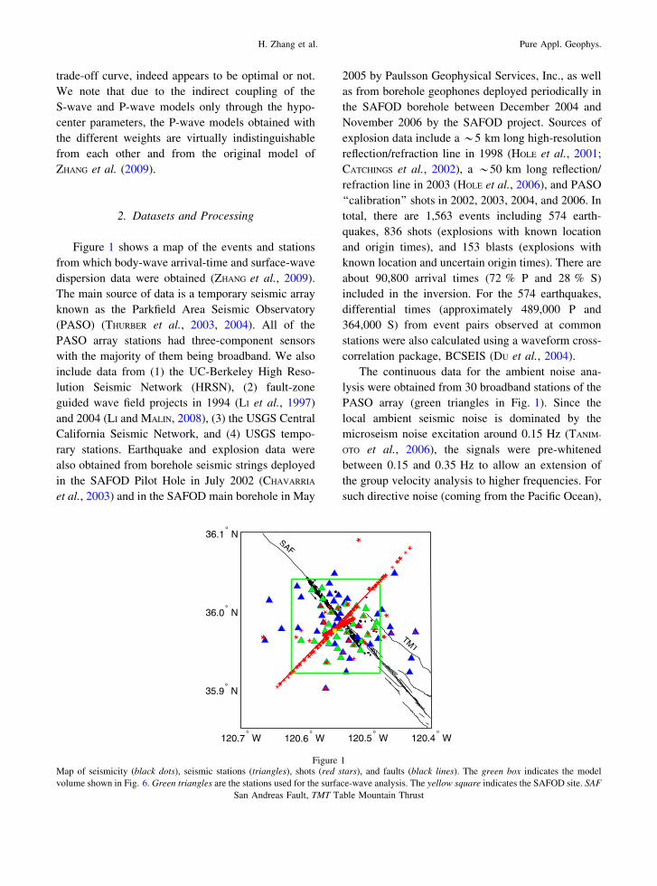
Figure 1 shows a map of the events and stations
from which body-wave arrival-time and surface-wave
dispersion data were obtained (ZHANG et al., 2009).
The main source of data is a temporary seismic array
known as the Parkfield Area Seismic Observatory
(PASO) (THURBER et al., 2003, 2004). All of the
PASO array stations had three-component sensors
with the majority of them being broadband. We also
include data from (1) the UC-Berkeley High Reso-
lution Seismic Network (HRSN), (2) fault-zone
guided wave field projects in 1994 (LI et al., 1997)
and 2004 (LI and MALIN, 2008), (3) the USGS Central
California Seismic Network, and (4) USGS tempo-
rary stations. Earthquake and explosion data were
also obtained from borehole seismic strings deployed
in the SAFOD Pilot Hole in July 2002 (CHAVARRIA
et al., 2003) and in the SAFOD main borehole in May
2005 by Paulsson Geophysical Services, Inc., as well
as from borehole geophones deployed periodically in
the SAFOD borehole between December 2004 and
November 2006 by the SAFOD project. Sources of
explosion data include a *5 km long high-resolution
reflection/refraction line in 1998 (HOLE et al., 2001;
CATCHINGS et al., 2002), a *50 km long reflection/
refraction line in 2003 (HOLE et al., 2006), and PASO
‘‘calibration’’ shots in 2002, 2003, 2004, and 2006. In
total, there are 1,563 events including 574 earth-
quakes, 836 shots (explosions with known location
and origin times), and 153 blasts (explosions with
known location and uncertain origin times). There are
about 90,800 arrival times (72 % P and 28 % S)
included in the inversion. For the 574 earthquakes,
differential times (approximately 489,000 P and
364,000 S) from event pairs observed at common
stations were also calculated using a waveform cross-
correlation package, BCSEIS (DU et al., 2004).
The continuous data for the ambient noise ana-
lysis were obtained from 30 broadband stations of the
PASO array (green triangles in Fig. 1). Since the
local ambient seismic noise is dominated by the
microseism noise excitation around 0.15 Hz (TANIM-
OTO et al., 2006), the signals were pre-whitened
between 0.15 and 0.35 Hz to allow an extension of
the group velocity analysis to higher frequencies. For
such directive noise (coming from the Pacific Ocean),
120.7 W 120.6 W 120.5 W 120.4 W
35.9 N
36.0 N
36.1 N
Figure 1Map of seismicity (black dots), seismic stations (triangles), shots (red stars), and faults (black lines). The green box indicates the model
volume shown in Fig. 6. Green triangles are the stations used for the surface-wave analysis. The yellow square indicates the SAFOD site. SAF
San Andreas Fault, TMT Table Mountain Thrust
H. Zhang et al. Pure Appl. Geophys.

the concept of passive seismic-noise tomography was
explored on three-component sensors (ROUX et al.,
2011). An optimal rotation algorithm (ORA) was
applied to the nine-component correlation tensor
measured from each pair of three-component seis-
mometers among the array, that forced each station
pair to re-align in the noise direction, a necessary
condition to extract unbiased travel-times from pas-
sive seismic processing (ROUX, 2009; ROUEFF et al.,
2009). Taking advantage of the short distances
between the sensors, only a relatively short time
period of data (15 days) was needed to obtain ade-
quate correlation results.
Note that no near-field contributions of the sur-
face-wave’s tensor were retrieved from the noise
correlation, as the dominant noise source was in the
far field. This confirmed that noise correlation on
long time records simply behaves as a time-domain
interferometer that magnifies phase coherence
between station pairs in the frequency bandwidth of
interest. As a consequence, the small size of the
seismic network is both an advantage and a disad-
vantage regarding tomography inversion: an
advantage as the coherence is high for many station
pairs, which makes travel time measurements very
accurate; a disadvantage since travel times extracted
from the noise-correlation tensor are close to zero,
which could make residual uncertainty of great
importance in velocity measurement errors. In prac-
tice, an average signal-to-noise ratio of 60 was
obtained at the peak maximum of the 15-day-aver-
aged correlation function for each station pair. With
such a high value of the signal-to-noise ratio, the
accuracy of the travel-time measurement could, in
theory, be close to infinity and, at least in practice,
sufficiently high to provide reliable estimations.
Finally, after the rotation was performed, an
optimal surface-wave tensor is obtained from which
Rayleigh and Love waves were separately extracted
for tomography inversion [see Fig. 2 and further
details about the Love-wave inversion in ROUX et al.
(2011)]. The choice of Love waves for the inversion
was motivated by (1) their high sensitivity to shallow
geophysical structure and (2) the residual pollution of
P-waves on the vertical and radial components (ROUX
et al., 2005) of the correlation tensor that may bias the
dispersion curve of Rayleigh waves. The tomography
inversion resulted from the combination of 360
selected dispersion curves for Love waves. Straight
rays were assumed as propagation paths and a 2.5-km
spatial smoothing was applied. The latter was based
on the point of minimum misfit as a function of spatial
smoothing length (Fig. 2). This shows that the sur-
face-wave group velocity maps were not heavily
smoothed. Examples of group velocity maps from
ROUX et al. (2011) are shown in Fig. 3. The northeast-
southwest velocity gradient across the San Andreas
Fault (SAF) is clearly visible in the ROUX et al. (2011)
Vs model, as well as the low-velocity region down to
*2.5 km below the surface between the SAFOD
borehole and the SAF surface trace.
3. Joint Inversion
First, we describe the basic elements of the (sep-
arate) body-wave and surface-wave inversions that
are incorporated into our joint inversion and then we
explain how the joint inversion is set up.
For this work, we make use of the regional-scale
version of the double-difference (DD) tomography
algorithm tomoDD (ZHANG and THURBER, 2003, 2006).
DD tomography is a generalization of DD location
(WALDHAUSER and ELLSWORTH, 2000), simultaneously
solving for the 3D velocity structure and seismic event
0 1 2 3 4 5 6 7 80.45
0.5
0.55
0.6
0.65
Spatial Smoothing Length (km)
Sur
face
Wav
e M
isfit
(s
2)
Figure 2Example misfit curve, for the 0.3 Hz band, for the determination of
the optimal spatial smoothing length for the Love wave group
velocity maps of ROUX et al. (2011) that are used in our joint
inversion. The plot indicates the minimum falls between 2.0 and
3.0 km, so a value of 2.5 km was adopted
Joint Inversion of Body-Wave Arrival Times and Surface-Wave Dispersion

locations. The P-wave and S-wave velocity models are
inverted for as separate models, although they are
mathematically coupled through the hypocenter
parameters. DD tomography uses a combination of
absolute and more accurate differential arrival times
and hierarchically determines the velocity structure
from larger scale to smaller scale. LSQR (PAIGE and
SAUNDERS, 1982) is used to invert for model pertur-
bations, and regularization of the inversion is
accomplished with a first-difference smoothing oper-
ator. The regional-scale version, tomoFDD (ZHANG
et al., 2004), employs a finite-difference solver [either
PODVIN and LECOMTE (1991), or HOLE and ZELT (1995),
the latter based on VIDALE (1988)] to calculate travel
times in a spherical Earth geometry that is converted to
a Cartesian system (so-called ‘‘sphere in a box’’).
The surface-wave inversion code that is integrated
into the joint inversion algorithm is from MACEIRA
and AMMON (2009) and follows JULIA et al. (2000).
The propagator matrix solver in the algorithm DIS-
PER80 (SAITO, 1988) is used for the forward
calculation of dispersion curves from layered velocity
models. Theoretically, the dispersion curve is a
function of shear wave velocity, compressional wave
velocity, and density of the media (BUCHER and
SMITH, 1971). However, the sensitivity to P-wave
velocity and density is significantly smaller than the
sensitivity to S-wave velocity (TAKEUCHI and SAITO,
1972; AKI and RICHARDS, 1980; BACHE et al., 1978;
TANIMOTO, 1991). Therefore, only shear velocity
variations are considered for modeling the Love wave
dispersion observations.
-120.6 -120.56 -120.52 -120.4835.92
35.94
35.96
35.98
36
36.02
36.04Love Wave - 0.15 Hz
1.0
1.5
2.0
2.5
-120.6 -120.56 -120.52 -120.4835.92
35.94
35.96
35.98
36
36.02
36.04Love Wave - 0.2 Hz
1.2
1.4
1.6
1.8
2.0
2.2
2.4
-120.6 -120.56 -120.52 -120.4835.92
35.94
35.96
35.98
36
36.02
36.04Love Wave - 0.25 Hz
1.0
1.2
1.4
1.6
1.8
2.0
2.2
-120.6 -120.56 -120.52 -120.4835.92
35.94
35.96
35.98
36
36.02
36.04Love Wave - 0.3 Hz
1.0
1.2
1.4
1.6
1.8
2.0
2.2
group velocity group velocity
group velocity group velocity
longitude longitude
latit
ude
latit
ude
Figure 3Example Love wave group velocity maps from ROUX et al. (2011) used in our joint inversion. Velocities are in m/s
H. Zhang et al. Pure Appl. Geophys.

To accomplish the joint inversion, the body-wave
and surface-wave equations are combined in a single
system with weighting factors controlling the relative
contributions of the two data types to the solution for
model perturbations. We note that, in general, the
body-wave equations involve the P-wave and S-wave
velocity structure and the source locations and/or
origin times (for earthquakes and explosions with
unknown origin time), whereas the surface-wave
equations only involve the S-wave velocity. Thus, the
joint inversion equations can be expressed as
l1GTp
H l1GTp
Vp0
l2GTs
H 0 l2GTs
Vs
0 0 l3GSWVs
0 wpLVp0
0 0 wsLVs
kHI 0 00 kpI 00 0 ksI
2666666666664
3777777777775
DHDmp
Dms
24
35 ¼
l1dTp
l2dTs
l3dSW
00000
266666666664
377777777775
;
ð1Þ
where GTp
H , GTs
H , GTp
Vpand GTs
Vsare the sensitivity
matrices of first P-arrival and S-arrival times with
respect to hypocenter parameters, Vp, and Vs,
respectively; GSWVs
is the sensitivity matrix of surface
wave dispersion data with respect to Vs; LVpand LVs
are the first-order smoothing matrices for the Vp and
Vs models with weights of wp and ws, respectively;
kH, kp, and ks are the damping parameters for hypo-
center parameters, Vp, and Vs model parameters,
respectively; DH, Dmp, and Dms are perturbations to
hypocenter parameters, Vp, and Vs model parameters,
respectively; and l1, l2 and l3 are relative weights
for body wave P-arrival and S-arrival times and
surface wave dispersion data, respectively. For sim-
plicity in our study we set data weights l1 and l2 for
P and S arrival time data to be equal. The damping
parameters, smoothing weight parameters, and data
weighting parameters are chosen by a combination of
requiring a reasonable condition number (mainly
controlled by the damping) and a trade-off analysis
(examining the data weighting). We retain the same
smoothing weight that was found to be optimal by
ZHANG et al. (2009). LSQR (PAIGE and SAUNDERS,
1982) is used to solve the system of Eq. (1).
We note that there is a difference in the way the
velocity structure is parameterized in the underlying
body-wave versus surface-wave components of the
joint inversion. For body-wave arrival times, the
velocity structure is represented by the value at grid
nodes, and interpolation is used to obtain the velocity
value at any point. Thus, velocity is treated as a
continuous function of position. In contrast, for the
surface waves, velocities are defined in latitude-lon-
gitude cells and vertical layers such that the velocity
is constant within each cell. To accommodate two
different model parameterizations, we put the node in
the center of each cell. For this study, the grid
intervals are 0.0048� in latitude and 0.0044� in lon-
gitude, and vary from 0.5 to 3 km in depth (at Z =
-0.5, 0, 0.5, 1.0, 2.0, 4.0, 7.0, and 10.0 km).
4. Trade-off Curve and Inversion Results
To explore specifically the effect of the joint
inversion on the structural model, we keep all data
and parameters constant except for the weighting of
the body-wave equations, which we vary over several
orders of magnitude, with the surface-wave weight
kept fixed at 1. We note that the damping and
smoothing we apply to stabilize LSQR and regularize
the inversion is the same as that used by ZHANG et al.
(2009) in their body-wave only tomography study.
We find that for weights below a value of 1 (i.e.,
equal weighting of body-wave and surface-wave
equations), the misfit to both the body-wave and
surface-wave data ceases to change, and above 100,
the body-wave misfit remains constant. Thus, we
consider the trade-off in data fit between body waves
and surface waves in the range 1–100 for the body-
wave weight (Fig. 4; Table 1). What we find is that
there is a strong, smooth variation in data fit as we
move from a weight of 1 to a weight of 100, with a
‘‘knee’’ in the curve near a weight of 20. Near this
point, a small increase in the body-wave weight leads
to a large increase in surface-wave misfit with little
decrease in body-wave misfit. Conversely, a small
decrease in the body-wave weight leads to a large
increase in body-wave misfit with little decrease in
surface-wave misfit. Thus, on this basis we tenta-
tively identify a body-wave weight of 20 as optimal.
An independent way to estimate the proper rela-
tive weighting of the body-wave and surface-wave
Joint Inversion of Body-Wave Arrival Times and Surface-Wave Dispersion

data is in terms of their relative data uncertainties.
For the body-wave data, the average pick uncertainty
is on the order of 0.02 s, based on the pick quality as
estimated directly from the waveform data, which
agrees well with the level of RMS misfit we obtain in
the trade-off analysis (Fig. 3). Similarly, the surface-
wave data uncertainty estimate of 10 % (ROUX et al.,
2011) is consistent with the RMS misfit on the order
of 0.2 km/s, given that the model velocities are
mainly in the range of 1.5–3 km/s. The ratio of 10
between these two uncertainties is of the same order
as the optimal weighting ratio of 20–1 from the trade-
off curve in Fig. 4. This is analogous to the stochastic
inverse (e.g., AKI et al., 1977), for which the ratio of
the a priori data variance to model variance is used as
the damping factor in the least squares inversion.
Next, we compare the inversion model results for
the nominal optimal body-wave weight (Fig. 5c) to
those for low (Fig. 5a), moderately low (Fig. 5b),
moderately high (Fig. 5d), and high (Fig. 5e) body-
wave weights. Horizontal slices through the Vs models
for the various cases are shown in Fig. 5 from 500 m
above to 2 km below sea level, where the changes are
greatest. Moving from the optimal (Fig. 5c) to the
moderately low (Fig. 5b) and low (Fig. 5a) body-
wave weight cases, the primary features remain
present but the model amplitude variations are slightly
reduced and smaller-scale features, especially those
near the SAF, shrink or disappear. This indicates the
lateral smoothing effect of the surface-wave data.
Moving from the optimal (Fig. 5c) to the moderately
high (Fig. 5d) and high (Fig. 5e) body-wave weight
cases, the primary features still remain, but there is a
substantial increase in the number and amplitude of
the smaller-scale features. Given that the body-wave
data misfit is reduced by only 4 % at the cost of a
*35–80 % increase in the surface-wave data misfit,
we interpret the higher-weight cases to indicate over-
fitting the noise in the body-wave data.
ROUX et al. (2011) highlighted a ‘‘U-shaped’’
feature containing a low-velocity zone in their
ambient noise model. We compare an iso-surface at
the same Vs value of 2.5 km/s in our new model
(Fig. 6a) to their original result (Fig. 6b). This steep-
sided wedge of slow material corresponds to the
sedimentary packages penetrated by the main SA-
FOD borehole. The joint inversion results reveal a
greater depth and along-fault extent of this feature
than the previous ambient noise only model.
We also note an area of strongly varying group
velocity with frequency in the southeast part of our
study area, near 35.97�, -120.50�, northeast of the
SAF (Fig. 3). Here, group velocity drops from
*2 km/s at 0.15 and 0.2 Hz to *1.2 km/s at 0.3 Hz.
This is an area that has been observed to be anoma-
lous in some previous studies. ZHANG et al. (2009)
found relatively high Vp here extending from *2 to
7 km depth from body-wave tomography, and ZHANG
et al. (2007) found the same area to be highly
anisotropic (*4 %) from a tomographic inversion of
shear wave splitting delays. Thus, it is not surprising
to find it to be anomalous in terms of Love wave
group velocity behavior as well.
Table 1
Variance reduction for body-wave and surface-wave data as a
function of the body-wave weight
Body-wave
weight
Body-wave variance
reduction (%)
Surface-wave variance
reduction (%)
1 77.5 74.0
2 77.7 73.9
5 78.4 73.0
20 79.7 61.6
50 80.4 28.7
100 81.1 1.15
Figure 4Plot of surface-wave data misfit (in km/s) versus body-wave data
misfit (in s) in the joint inversion as a function of the body-wave
weight (the surface-wave weight was kept fixed at 1). A body-wave
weight of 20 is adopted as optimal
H. Zhang et al. Pure Appl. Geophys.

−120.6−120.55
−120.5 35.92 35.94 35.96 35.98 36 36.02
−2
−1.5
−1
−0.5
0
0.5
Dep
th (
km)
LatitudeLongitude
1
1.5
2
2.5
3
3.5
4
−120.6−120.55
−120.5 35.92 35.94 35.96 35.98 36 36.02
−2
−1.5
−1
−0.5
0
0.5
Dep
th (
km)
LatitudeLongitude
1
1.5
2
2.5
3
3.5
4
−120.6−120.55
−120.5 35.92 35.94 35.96 35.98 36 36.02
−2
−1.5
−1
−0.5
0
0.5
Dep
th (
km)
LatitudeLongitude
1
1.5
2
2.5
3
3.5
4
−120.6−120.55
−120.5 35.92 35.94 35.96 35.98 36 36.02
−2
−1.5
−1
−0.5
0
0.5
Dep
th (
km)
LatitudeLongitude
1
1.5
2
2.5
3
3.5
4
−120.6−120.55
−120.5 35.92 35.94 35.96 35.98 36 36.02
−2
−1.5
−1
−0.5
0
0.5
Dep
th (
km)
LatitudeLongitude
1
1.5
2
2.5
3
3.5
4
(a) (b)
(c) (d)
(e)
Figure 5Comparison of velocity model results for different body-wave weights, showing horizontal slices at the depths of the shallow grid nodes
(-0.5, 0, 0.5, 1, and 2 km depth relative to mean sea level). The weights used for the models that are shown: (a) 2, (b) 5, (c) 20, (d) 50,
(e) 100. The black line is the SAF trace. The view is from the southeast
Joint Inversion of Body-Wave Arrival Times and Surface-Wave Dispersion

5. Discussion and Conclusions
The joint inversion algorithm expressed by Eq. (1)
has advantages compared to separate body-wave
arrival time inversion and surface-wave dispersion
inversion. Compared to the separate arrival-time
inversion, the joint inversion Vs model is more strongly
constrained by the combination of body-wave data and
surface-wave data. Even though traditional surface-
wave inversion typically only derives a Vs model, an
updated Vp model is required at each iteration in order
to compute the surface wave responses. In traditional
Figure 6Iso-surface view of the 2.5 km/s Vs surface for (a) the weight of 20 model in Fig. 5 compared to (b) the same view from ROUX et al. (2011).
The view is from the northwest. Notice the deeper expression and longer extent of the ‘‘U-shaped’’ feature in the joint inversion model in (a)
H. Zhang et al. Pure Appl. Geophys.

surface-wave inversions, this is generally accom-
plished by assuming a constant Vp/Vs ratio provided by
the a priori model. In comparison, the joint inversion
determines a more reliable Vp model from P-wave
arrival times. As a result, the surface-wave responses
are more accurate and the surface-wave data can be
better used to invert for the Vs model.
The joint inversion results do not make significant
changes to the main features found previously in the
crust surrounding SAFOD. Rather, the joint inversion
suppresses oscillatory features in the Vs model that do
not make a significant change in the fit to the body-
wave data. Adding the surface-wave constraints to
the body-wave inversion leads to a simpler
(smoother) Vs model that is able to fit both the body-
wave and surface-wave data adequately.
Acknowledgments
We thank Yehuda Ben-Zion and Antonio Rovelli for
organizing the 40th Workshop of the International
School of Geophysics on ‘‘Properties and Processes
of Crustal Fault Zones’’ in Erice, Sicily, which
motivated the present work. We are grateful to two
anonymous reviewers for their constructive com-
ments, which we hope have led to substantial
improvement of the manuscript. This research pre-
sented here was partly supported by the Chinese
government’s executive program for exploring the
deep interior beneath the Chinese continent (SinoP-
robe-02), Natural Science Foundation of China under
Grant No. 41274055, and Fundamental Research
Funds for the Central Universities (WK2080000053).
This research was also supported by DE-NA0001523
from the US Department of Energy.
REFERENCES
AKI, K., A. CHRISTOFFERSSON, and E.S. HUSEBYE (1977). Determi-
nation of the three-dimensional structure of the lithosphere, J.
Geophys. Res., 82, 277–296.
AKI, K., and P. G. RICHARDS (1980). Quantitative Seismology:
Theory and Methods, W. H. Freeman, San Francisco, CA, USA.
BACHE, T. C., W. L. RODI, and D. G. HARKRIDER (1978). Crustal
structures inferred from Rayleigh-wave signatures of NTS
explosions, Bull. Seismol. Soc. Am., 68, 1399–1413.
BECKEN, M., O. RITTER, S. K. PARK, P. A. BEDROSIAN, U. WECKMANN,
and M. WEBER (2008), A deep crustal fluid channel into the San
Andreas Fault system near Parkfield, California, Geophys. J. Int.
173, 718–732.
BENNINGTON, N., C. THURBER, and S. ROECKER (2008), Three-dimen-
sional seismic attenuation structure around the SAFOD site,
Parkfield, California, Bull. Seismol. Soc. Am. 98, 2934–2947.
BENNINGTON, N., H. ZHANG, C. H. Thurber, and PAUL A. BEDROSIAN
(in revision), Joint inversion of seismic and magnetotelluric data
in the Parkfield region of California using the normalized cross-
gradient constraint, Pure App. Geophys.
BEN-ZION, Y., and P. MALIN (1991), San Andreas fault zone head
waves near Parkfield, California. Science 251, 1592–1594.
BLEIBINHAUS, F., J. A. HOLE, T. RYBERG, and G. S. FUIS (2007),
Structure of the California Coast Ranges and San Andreas Fault
at SAFOD from seismic waveform inversion and reflection
imaging, J. Geophys. Res. 112, B06315, doi:10.1029/
2006JB004611.
BUCHER, R. L., and R. B. SMITH (1971). Crustal structure of the
eastern Basin and Range Province and the northern Colorado
Plateau from phase velocities of Rayleigh waves, in The Struc-
ture and Physical Properties of the Earth’s Crust, Geophys.
Monogr. Ser., vol. 14, edited by J. G. Heacock, pp. 59–70, AGU,
Washington, D.C.
CATCHINGS, R. D., M. J. RYMER, M. R. GOLDMAN, J. A. HOLE, R.
HUGGINS and C. LIPPUS (2002), High-resolution seismic velocities
and shallow structure of the San Andreas Fault Zone at Middle
Mountain, Parkfield, California, Bull. Seismol. Soc. Am. 92,
2493–2503.
CHAVARRIA, J. A., P. MALIN, R. D. CATCHINGS, and E. SHALEV
(2003), A look inside the San Andreas fault at Parkfield through
vertical seismic profiling, Science 302, 1746–1748.
DU, W.-X., C. H. THURBER, and D. EBERHART-PHILLIPS (2004),
Earthquake relocation using cross-correlation time delay esti-
mates verified with the bispectrum method, Bull. Seismol. Soc.
Am. 94, 856–866.
EBERHART-PHILLIPS, D., and A. J. MICHAEL (1993), Three-dimen-
sional velocity structure, seismicity, and fault structure in the
Parkfield region, central CA, J. Geophys. Res. 98,
15,737–15,758.
HOLE, J. A., R. D. CATCHINGS, K. C. St. CLAIR, M. J. RYMER, D. A.
OKAYA, and B. J. CARNEY (2001), Steep-dip imaging of the
shallow San Andreas fault near Parkfield, Science 294,
1513–1515.
HOLE, J., T. RYBERG, G. FUIS, F. BLEIBINHAUS, and A. SHARMA
(2006), Structure of the San Andreas fault zone at SAFOD from a
seismic refraction survey, Geophys. Res. Lett. 33, L07312.
HOLE, J. A., and ZELT, B. C. (1995), 3-D finite-difference reflection
traveltimes, Geophys. J. Int. 121, 427–434.
JULIA, J., C. J. AMMON, R. B. HERRMANN, and A. M. CORREIG (2000),
Joint inversion of receiver function and surface wave dispersion
observations, Geophys. J. Int. 143, 99–112.
KORNEEV, V. A., R. M. NADEAU, and T. V. MCEVILLY (2003),
Seismological studies at Parkfield IX: Fault-zone imaging using
guided wave attenuation, Bull. Seismol. Soc. Am. 93,
1415–1426.
LEES, J. M., and P. E. MALIN (1990), Tomographic images of P
wave velocity variation at Parkfield, California, J. Geophys. Res.
95, 21,793–21,804.
LEWIS, M. A., and Y. BEN ZION (2010), Diversity of fault zone
damage and trapping structures in the Parkfield section of the
San Andreas Fault from comprehensive analysis of near fault
seismograms, Geophys. J. Int. 183, 1579–1595.
Joint Inversion of Body-Wave Arrival Times and Surface-Wave Dispersion

LI, Y.-G., W. L. ELLSWORTH, C. H. THURBER, P. MALIN, and K. AKI
(1997), Fault zone guided waves from explosions in the San
Andreas fault at Parkfield and Cienega Valley, California, Bull.
Seism. Soc. Am. 87, 210–221.
LI, Y.-G., and P.E. MALIN (2008), San Andreas Fault damage at
SAFOD viewed with fault-guided waves, Geophys. Res. Lett. 35,
L08304, doi:10.1029/2007GL032924.
LI, Y. G., P. C. LEARY, K. AKI, and P. E. MALIN (1990), Seismic
trapped modes in Oroville and San Andreas fault zones, Science
249, 763–766.
LI, Y.-G., J. E. VIDALE, and E. S. COCHRAN (2004), Low-velocity
damaged structure of the San Andreas Fault at Parkfield from
fault zone trapped waves, Geophys. Res. Lett. 31, L12S06,
doi:10.1029/2003GL019044.
MICHELINI, A., and T.V. MCEVILLY (1991), Seismological studies at
Parkfield: I, Simultaneous inversion for velocity structure and
hypocenters using cubic B-splines parameterization, Bull. Seism.
Soc. Am. 81, 524–552.
MACEIRA, M. and C. J. AMMON (2009). Joint inversion of surface
wave velocity and gravity observations and its application to
Central Asian basins shear velocity structure, J. Geophys. Res.
114, B02314, doi:10.1029/2007JB005157.
PAIGE, C. C., and M. A. SAUNDERS (1982), LSQR: An algorithm for
sparse linear equations and sparse least squares, ACM Trans.
Math. Software 8, 43–71.
PODVIN, P. and I. LECOMTE (1991), Finite difference computation of
traveltimes in very contrasted velocity models: a massively
parallel approach and its associated tools., Geophys. J. Int. 105,
271–284.
ROECKER, S., C. THURBER, and D. MCPHEE (2004), Joint inversion of
gravity and arrival time data from Parkfield: New constraints on
structure and hypocenter locations near the SAFOD drill site,
Geophys. Res. Lett. 31, L12S04.
ROECKER, S., C. THURBER, K. ROBERTS, and L. POWELL (2006),
Refining the image of the San Andreas Fault near Parkfield,
California using a finite difference travel time computation
technique, Tectonophysics 426, doi:10.1016/j.tecto.2006.02.026.
ROUX, P., K.G. SABRA, P. GERSTOFT and W.A. KUPERMAN (2005), P-
waves from cross-correlation of seismic ambient noise, Geophys.
Res. Lett. 32, L19303.
ROUEFF A., P. ROUX and P. REFREGIER (2009), Wave separation in
ambient seismic noise using intrinsic coherence and polarization
filtering, Signal Process. 89, 410–421.
ROUX, P. (2009), Passive seismic imaging with directive ambient
noise: Application to surface waves on the San Andreas Fault
(SAF) in Parkfield, Geophys. J. Int. 179, 367–373.
ROUX, P., A. ROUEFF and M. WATHELET (2011), The San Andreas
Fault revisited through seismic noise and surface-wave tomog-
raphy, Geophys. Res. Lett., 38, L13319.
SAITO, M. (1988), DISPER80: A subroutine package for the cal-
culation of seismic normal mode solutions, in D. J. Doornbos
(ed.), Seismological Algorithms: Computational Methods and
Computer Programs, Academic Press, New York, pp. 293–319.
TAKEUCHI, H., and M. SAITO (1972), Seismic surface waves, in
Methods of Computational Physics, edited by B. A. Bolt,
pp. 217–295, Academic, New York.
TANIMOTO, T. (1991), Waveform inversion for three-dimensional
density and S-wave structure, J. Geophys. Res., 96, 8167–8189.
TANIMOTO, T., S. ISHIMARU, and C. ALVIZURI (2006), Seasonality of
particle motion of microseisms, Geophys. J. Int. 166, 253–266,
doi:10.1111/j.1365-246X.2006.02931.x.
Thurber, C., S. Roecker, K. Roberts, M. Gold, L. Powell, and K.
Rittger (2003), Earthquake locations and three-dimensional fault
zone structure along the creeping section of the San Andreas
fault near Parkfield, CA: Preparing for SAFOD, Geophys. Res.
Lett. 30.
THURBER, C., S. ROECKER, H. ZHANG, S. BAHER, and W. ELLSWORTH
(2004), Fine-scale structure of the San Andreas fault zone and
location of the SAFOD target earthquakes, Geophys. Res. Lett.
31, L12S02.
UNSWORTH M, and P. BEDROSIAN (2004) Electrical resistivity at the
SAFOD site from magnetotelluric exploration, Geophys. Res.
Lett. 31, L12S05, doi:10.1029/2003GL019405.
UNSWORTH M, P. BEDROSIAN, M. EISEL, G. EGBERT, and W. SIRI-
PUNVARAPORN (2000) Along strike variations in the electrical
structure of the San Andreas Fault at Parkfield, California,
Geophys. Res. Lett. 27, 3021–2024.
UNSWORTH, M. J., P. E. MALIN, G. D. EGBERT, and J. R. BOOKER
(1997), Internal structure of the San Andreas fault zone at
Parkfield, California, Geology 25, 359–362.
VIDALE, J. (1988), Finite-difference calculation of travel times,
Bull. Seis. Soc. Am. 78, 2062–2076.
WALDHAUSER, F., and W. L. ELLSWORTH (2000). A double-difference
earthquake location algorithm: method and application to the
northern Hayward Fault, California, Bull. Seism. Soc. Am. 90,
1353–1368.
WU, J., J. A. HOLE, and J. A. SNOKE (2010), Fault zone structure at
depth from differential dispersion of seismic guided waves:
evidence for a deep waveguide on the San Andreas Fault, Geo-
phys. J. Int. 182, 343–354.
ZHANG, H., and C. H. THURBER (2003), Double-difference tomog-
raphy: The method and its application to the Hayward Fault,
California, Bull. Seism. Soc. Am. 93, 1875–1889.
ZHANG, H., and C. THURBER (2005). Adaptive mesh seismic
tomography based on tetrahedral and Voronoi diagrams: Appli-
cation to Parkfield, California, J. Geophys. Res. 110, B04303.
ZHANG, H., and C. THURBER (2006). Development and applications
of double-difference tomography, Pure App. Geophys. 163,
373–403, doi:10.1007/s00024-005-0021-y.
ZHANG, H., Y. LIU, C. THURBER, and S. ROECKER (2007), Three-
dimensional shear-wave splitting tomography in the Parkfield,
California Region, Geophys. Res. Lett. 34, L24308. doi:10.1029/
2007GL03195.
ZHANG, H., C. THURBER, and P. BEDROSIAN (2009), Joint inversion
for Vp, Vs, and Vp/Vs at SAFOD, Parkfield, California, Geochem.
Geophys. Geosyst. 10, Q11002, doi:10.1029/2009GC002709.
ZHANG, H., C. THURBER, D. SHELLY, S. IDE, G. BEROZA, and A.
HASEGAWA (2004), High-resolution subducting slab structure
beneath Northern Honshu, Japan, revealed by double-difference
tomography, Geology 32, 361–364.
(Received September 14, 2013, revised February 17, 2014, accepted February 19, 2014)
H. Zhang et al. Pure Appl. Geophys.