Joint Identification of Multiple Tracked...

CAN UNCLASSIFIED

Defence Research and Development Canada External Literature (P) DRDC-RDDC-2017-P073 September 2017

CAN UNCLASSIFIED

Joint Identification of Multiple Tracked Targets

Dominic E. Schaub DRDC – Atlantic Research Centre Journal of Advances in Information Fusion Volume 12 Issue number 1 pp. 20–40 Date of Publication from Ext Publisher: June 2017

Terms of Release: This document is approved for Public release.

CAN UNCLASSIFIED

Template in use: P14-0708-1207 - cover.dotm

© Her Majesty the Queen in Right of Canada (Department of National Defence), 2017

© Sa Majesté la Reine en droit du Canada (Ministère de la Défense nationale), 2017

CAN UNCLASSIFIED

IMPORTANT INFORMATIVE STATEMENTS

Disclaimer: This document is not published by the Editorial Office of Defence Research and Development Canada, an agency of the Department of National Defence of Canada, but is to be catalogued in the Canadian Defence Information System (CANDIS), the national repository for Defence S&T documents. Her Majesty the Queen in Right of Canada (Department of National Defence) makes no representations or warranties, express or implied, of any kind whatsoever, and assumes no liability for the accuracy, reliability, completeness, currency or usefulness of any information, product, process or material included in this document. Nothing in this document should be interpreted as an endorsement for the specific use of any tool, technique or process examined in it. Any reliance on, or use of, any information, product, process or material included in this document is at the sole risk of the person so using it or relying on it. Canada does not assume any liability in respect of any damages or losses arising out of or in connection with the use of, or reliance on, any information, product, process or material included in this document.

This document was reviewed for Controlled Goods by Defence Research and Development Canada (DRDC) using the Schedule to the Defence Production Act.

Joint Identification of Multiple

Tracked Targets

DOMINIC E. SCHAUB

This paper derives a rigorously Bayesian technique for estimat-

ing the identities of a plurality of targets that are well separated or

tracked using the (joint) probabilistic data association filter. In con-

trast to the single-target classification problem, the joint identifica-

tion of multiple targets is characterized by statistical dependencies

between track-to-identity assignments that render track-level esti-

mation of identity suboptimal. The present method rigorously ac-

counts for these dependencies and allows arbitrary feature and kine-

matic measurements generated by individual targets to be used in

finding the statistically-optimal track-to-identity assignment proba-

bilities. The problem is decomposed into global combinatorial iden-

tity deconfliction and local target tracking and classification that is

based on a unified measure-theoretic filtering framework. The com-

putational complexity of this technique is shown to be dominated by

calculation of the permanent of a non-negative matrix, which may

be found exactly in exponential time or approximated in polyno-

mial time using Markov chain Monte Carlo methods. Strategies for

improving numerical performance are given for cases where certain

subsets of targets are indistinguishable or unobservable. This work

is relevant to applications in tactical settings, surveillance, including

video tracking, air/land/maritime situational awareness, and auto-

mated intelligence collection.

Manuscript received February 25, 2015; revised February 7, 2016;

released for publication June 21, 2016.

Refereeing of this contribution was handled by Dr. Paolo Braca.

Author’s address: Defence Research and Development Canada, At-

lantic Research Centre, 9 Grove St., P.O. Box 1012, Dartmouth NS

B2Y 3Z7 Canada (E-mail: [email protected]).

This work was supported by DRDC Applied Research Project 06eo,

Situational Information for Enabling Development of Northern Aware-

ness (SEDNA).

1557-6418/17/$17.00 c° 2017 JAIF

1. INTRODUCTION

Multisensor tracking is a branch of information fu-

sion that appears in many domains that require sit-

uational awareness, such as air traffic control, video

surveillance, and missile defence. The fundamental task

in tracking involves estimating target kinematic states

(such as position and/or velocity of an aircraft) from a

time series of measurements generated by a suite of one

or more sensors (e.g. radar). While several approaches

have been developed for fusing measurement data, those

based on (or approximating) Bayesian filtering [1]—[3]

have enjoyed the widest adoption owing to their rig-

orous treatment of sensor error and target dynamics.

In the Bayesian framework, a probability distribution

over target state space is maintained and updated with

new measurements using Bayes’ theorem. In particular,

where sensor noise and target dynamics admit a priori

statistical characterizations, Bayesian methods offer a

rigorously mathematical framework for computing op-

timal statistical estimates.

Over the course of several decades, enormous ad-

vances in sensors, communications systems, and com-

puting power have enabled the development of a con-

siderable number of tracking methods, from the simple,

linear Kalman filter [4], [5] (which solves the single-

target state-estimation problem under Gaussian condi-

tions) to the sophisticated multi-hypothesis tracker [6]

(which performs the task of associating multiple ob-

servations to multiple tracks and is used in conjunction

with a collection of individual filters) and the probability

hypothesis density (PHD) filter [7], [8] (which tightly

integrates data association and filtering). Research has

also broadened to include the related problems of target

identification and classification, which naturally extend

the mathematics of target tracking. In principle, these

undertakings may be regarded as specializations of the

same fundamental problem, as identification amounts to

a constrained form of classification that assigns a given

class to at most a single target.

As with tracking, identification and classification are

marked by significant differences between their single-

and multiple-target specializations. Single-target joint

tracking and classification (JTC) has been extensively

studied as a rigorously Bayesian problem, with detailed

theoretical derivations provided in [9]—[11]. Particular

attention has been given to exploiting kinematic data to

assist classification, including [12], which demonstrated

improvements in classification performance by apply-

ing a second-order uncertainty model to the mapping

between the feature and target class spaces. Similarly,

[13] developed a framework of multiple-model particle

and mixture Kalman filters subject to kinematic con-

straints and subsequently considered its application to

discriminating between commercial and military aircraft

20 JOURNAL OF ADVANCES IN INFORMATION FUSION VOL. 12, NO. 1 JUNE 2017

using radar contacts. In [14], it was shown that maxi-

mum entropy techniques can significantly improve ac-

curacy in Bayesian classification characterized by epis-

temic uncertainty in the prior (which, when unknown, is

typically taken as uniform). Specific applications have

also been considered, including a decision-theoretical

problem of identifying aircraft using radar measure-

ments [15] and a joint tracking and classification frame-

work for radar and electronic-support-measure obser-

vations [16]. It is worth highlighting that Bayesian

single-target joint tracking and classification is typi-

cally computationally feasible for modest-dimensional

problems, where the ‘curse of dimensionality’ (in the

non-parametric case) is usually mild and may be over-

come through particle filtering or carefully implemented

fixed-grid discretizations.

In the multitarget context, identification has been

theoretically analyzed as an extension to Finite Set

Statistics (FISST) using the framework of labelled ran-

dom sets [17]. Several approximation schemes have

also been developed (albeit lacking in rigorous track-

ing formalism), including methods based on informa-

tion theory [18], [19] and Sinkhorn rescaling [20]—

[22]. Accounts of relating specific tracking implemen-

tations with the higher-level identification problem have

been given in [23], which developed (using a series

of approximations) a multitarget Kalman filter that uti-

lizes target identity information. In particular, a group-

theoretical Fourier method [24]—[26] has emerged as

a general framework for approximate reasoning over

combinatorial matchings. In this approach, distribu-

tions defined over the set of permutations are replaced

with equivalent (Fourier-transformed) distributions over

the irreducible representations of the related symmet-

ric group. Under favourable conditions, the transformed

quantities may be approximated with a small number

of terms, thereby avoiding the factorial space and time

complexities ordinarily encountered in combinatorial

problems.

The foregoing methods of multitarget identification

are either intractable (implementation of the random-set

formulation entails further numerical simplifications) or

dependent on complex approximations that impede the

analysis of error in computed estimates. These limita-

tions are a consequence not only of the inherent com-

plexity of multitarget tracking, but of the fact that mul-

titarget identification and constrained classification–

where at most a fixed number of targets may belong to

a given class1–, is itself non-local and combinatorial,

as estimating the class of a target depends partly on ob-

servations made at distant tracks (e.g. a target at a given

track is unlikely to be a particular identity when there

is strong evidence for its presence elsewhere). Interest-

ingly, the underlying mathematical structure–known as

1For example, a given task group may include a known number of

UAVs and helicopters. In this case, the fixed number of each aircraft

imposes a global constraint on the multitarget classification problem.

the assignment problem [27], [28]–is of considerable

generality, appearing in several diverse contexts such

as economics [29], [30], operations research [31], [32],

and the joint probabilistic data association (JPDA) fil-

ter [33].

The present work develops a special case of rigor-

ously Bayesian multitarget identification and classifi-

cation wherein it becomes computationally feasible to

calculate nearly exact estimates of identity and kine-

matic states. The necessary conditions are met when-

ever measurement-to-track associations are unambigu-

ous, i.e., where tracks are well separated or, alterna-

tively, where (J)PDA is used to resolve the data asso-

ciation problem. The primary objectives motivating this

work lie with computing the marginal track-to-identity

assignments in the form of posterior probabilities that a

given identity–such as a vessel with a particular regis-

tration number–is present at a track of interest (Fig. 1)

and, in addition, finding the optimal posterior target-

state-space densities from which kinematic estimates

may be calculated. It is shown that the algorithmic bot-

tleneck stems from calculation of the matrix permanent,

a standard function in combinatorics and one that may

be efficiently computed using rapidly-mixing Markov

chain Monte Carlo (MCMC) methods [34]—[36]. As

these techniques yield approximations whose residual

errors decrease exponentially with iteration number, op-

timal Bayesian estimates of any quantity may therefore

be found to machine precision in polynomial time. It

is further shown that the Ryser method [37], [38] (an

analytical permanent algorithm) can be extended to ex-

ploit the mathematical structure present when targets

form classes of indistinguishable members, a result that

enables the exact constrained classification of very large

numbers of targets to be performed efficiently.

The remainder of this paper is organized as fol-

lows. Section 2-A derives a general Bayesian frame-

work that unifies the problems of tracking, classifica-

tion, and identification under a single statistical system

that fully accounts for their complex mathematical inter-

dependence and makes optimal use of arbitrary feature

and kinematic observations originating from individual

tracks. In §2-B, the framework is equipped with sim-

plifying conditions, including the requirement for un-

ambiguous measurement-to-track associations, which in

turn give way to an efficient factorization of the joint

target density. This factorization naturally partitions the

framework into the connected problems of local track-

ing and classification and global combinatorial decon-

fliction of identity, thereby significantly improving the

associated time and space complexities. Section 2-C

proceeds to show that the central task of deconflic-

tion amounts to computing the permanent of a non-

negative matrix, and in §2-D, the framework is extended

to applications where data association is performed with

(J)PDA. Section 3 then discusses algorithms for com-

puting the matrix permanent, including a Ryser method

that is modified to exploit the presence of unobservable

JOINT IDENTIFICATION OF MULTIPLE TRACKED TARGETS 21

Fig. 1. Simplified overview of the problem studied in this paper.

Given a set T of tracks with associated observations (a) and a

second set I of unique identities, it is desired to find the matrix of

posterior marginal track-to-identity assignment probabilities (b).

or indistinguishable targets to improve runtime (§3-A

and §3-B) and various approximation methods, includ-

ing Markov chain Monte Carlo techniques and loopy

belief propagation (§3-C). Finally, a series of numerical

examples are considered in §4, demonstrating how this

work may be applied to benefit situational awareness.

2. BAYESIAN FORMULATION

A. Overview

This section derives a measure-theoretic Bayesian

framework for multitarget filtering and classification in

cases where target dynamics and measurements satisfy

standard Markov conditions. Development proceeds by

augmenting the conventional analytical representation

of Bayesian multitarget tracking [8] with a singular-

measure extension that allows seamless integration of

classification based on static attributes. In what follows,

an ‘identity’ refers to a physical entity of uncertain lo-

cation that possesses a known signature, which can be

represented by a combination of dynamic and static fea-

tures.2 Consistent with conventional tracking nomencla-

ture, ‘target’ denotes the entity present at a given track,

which is localized to a particular region in space but is of

2For example, each registered vessel on a lake would constitute a

unique identity. Note that for a given suite of sensors, identities may

not necessarily be distinguishable by way of their observed signatures,

as occurs when identical models of watercraft are tracked with radar.

In practical applications, the set of identities may be realized as a

comprehensive database of physical assets (and their signatures) that

could be encountered by the tracking system.

uncertain identity. The sets of all tracks and identities in

existence are designated T and I, respectively (Fig. 1).

Furthermore, these sets are well ordered, allowing each

of their members to be referenced by a unique integer

index.

The present framework is simplified when each

identity is assignable to a distinct track. To accommo-

date circumstances where observed tracks are produced

by a series of false alarms (or where there are fewer

observed tracks than identities), it may be mathemat-

ically convenient to enlarge T by including additional

tracks whose targets are never observed. Without loss

of generality, the total set of tracks may thus be defined

by the union

T = TO [TH (1)

where TO are those tracks with observed targets (to

which one or more measurements are associated), and

TH is a (possibly empty) set of hidden tracks lacking

measurements. The set TH can be made identical in size

to I to allow for the possibility that every track in TOwas generated by false alarms.

Each identity i 2 I assumes values in its associatedstate space (Si). For mathematical simplicity, an arbi-trary identity state xi 2 Si is made to encapsulate bothdynamic attributes (e.g. velocity) and static properties

(e.g. length) in a manner that allows the state space to

be decomposed as the Cartesian product

Si = Si,d£Si,s (2)

where Si,d and Si,s are the dynamic and static compo-nents, respectively. Both Si,d and Si,s must be equippedwith ¾-algebras, allowing Si to be assigned the measure

¹i(W) = ¸i(prdW)£ ±i(prsW) (3)

where W μ Si is an arbitrary measurable set, pr(¢) areprojection operators, and ¸i(¢) and ±i(¢) are measureson Si,d and Si,s, respectively. The latter is the (singular)Dirac measure that encodes the given identity’s static at-

tribute information. For example, where there exist two

identities of length 1 m and 2 m, their respective Dirac

measures on their ‘length’ spaces would be ±1 m(¢) and±2 m(¢). For an observation of target length given by3N (¹= 1 m,¾2 = 1 m2), the likelihoods associated witheach of the identities may be found by applying their

Dirac measures to the measurement’s pdf, and are thus

(2¼)¡1=2 and e¡1(2¼)¡1=2 for the 1-m and 2-m identi-

ties, respectively. However, rather than extracting fea-

ture information directly from individual observations,

it may be convenient to maintain a running product

of static-feature measurements from previous updates–

these products are simply individual measurements pdfs

(pmfs) that are combined by successive applications of

3Obviously, the normal distribution implies that lengths could assume

negative (non-physical) values.


Bayes’ rule.4 Invocation of the identity-specific Dirac

measures may then be deferred to the time at which the

posterior probabilities are computed. By transferring the

classification operations to the measure, static features

are placed on equal footing as the dynamic components,

allowing Bayesian feature measurement updates to be

performed in manner identical to their kinematic coun-

terparts. Note that this formulation simplifies the subse-

quent presentation but is theoretically equivalent to that

derived with intermediate feature spaces.

Multitarget tracking and classification may be for-

mulated with Cartesian products of individual identity

spaces that are constructed as

SJ =Yi2JSi, J μ I, (4)

where the product order is given by the total order on

I, and the subscripts are suppressed when J = I. The

SJ of (4) are similarly assigned the family of productmeasures

¹J (W) =Yi2J¹i(priW): (5)

Uncertainty in the system’s dynamic state may be rep-

resented with a random variable X on S whose proba-bility density function pX(x) is uniquely defined up toan equivalence class determined by the measures of (3).

In particular, each equivalence class contains a member

that assumes strictly constant values on each of the static

attribute spaces and thus satisfies

pXi(xi) = pXi(x0i),

8xi,x0i 2 S : prdfxig= prdfx0ig (6)

which uses the fact that all functions on the ith static

attribute space that evaluate to the same quantity for

the argument selected by ±i(¢) are equivalent under theassociated measure (e.g. f1(x) = 1=

p2, f2(x) = jsin(x)j,

and f3(x) = jcos(x)j are equivalent under ±¼=4(¢)). Priorson static attribute spaces may therefore be specified as

constant functions. Marginalization of this density with

respect to J ½ I may be defined as

pXInJ (xInJ ) =ZSJpX(x)d¹J (xJ ): (7)

The system state is updated with a sequence of

discrete-time measurements Zk, which are samples of

4Philosophically, this approach treats fixed features (such as length)

as time-indexed probability distributions (akin to the distributions de-

scribing kinematics) subject to standard Bayesian recursive filtering.

By choosing the prior feature density to be the Dirac delta function (or

Kronecker delta function where the prior is a pmf) and defining the

associated Markov transitions to have no effect, the feature posterior

will remain the Dirac delta function indefinitely, as no measurement

function can increase its information further. However, the delta func-

tion’s magnitude will be scaled in accordance with how ‘close’ the

feature measurements are to the feature encoded in the delta function.

The Dirac measure is substituted for the Dirac delta function to avoid

the mathematical sophistication required to use the latter.

the time series of random variables Zk 2 SZ that describethe measurement processes. The collection of measure-

ments up to and including the kth time step is given by

Z1:k = fZk0 gkk0=1: (8)

For each time step there exists a likelihood function

f : (SZ ,S)! [0,1) that carries information on the mea-sured static and/or dynamic attributes. When condi-

tioned on the multitarget state and evaluated for a given

measurement Zk = Zk, this function may be written as

fZk jXk (Zk j x): (9)

Between measurements, the dynamic components of

the state are projected forward in time by a Markov tran-

sition density f : (S,S)! [0,1) that encodes the knownaspects of the identities’ dynamics (e.g. acceleration,

etc.). It is similarly conditioned on the kth state and

is denoted byfXk+1jXk (x j x0): (10)

Bayesian filtering consists of alternately updating the

state with new measurements using Bayes’ rule (usu-

ally increasing the Fisher information) and transitioning

the state forward in time (usually decreasing the infor-

mation). The measurement and transition steps may be

written as

pXk jZ1:k (x j Z1:k) =fZk jXk (Z

k j x)pXk jZ1:k¡1 (x j Z1:k¡1)RSfZk jXk (Z

k j x0)pXk jZ1:k¡1 (x0 j Z1:k¡1)d¹(x0)(BF.1)

and

pXk+1jZ1:k (x j Z1:k) =ZSfXk+1jXk (x j x0)pXk jZ1:k (x0 j Z1:k)d¹(x0)

(BF.2)

respectively. By virtue of the product measures of (3),

these equations simultaneously subsume both tracking

and classification (two specializations that occur in the

absence of Ss,i and Sd,i, respectively).

B. Tracking and Identification of Well-SeparatedTargets

The general framework of the previous section is

challenging to implement numerically. For example, a

fixed-grid discretization of a probability density func-

tion exhibits time and space (storage) complexities5 that

scale exponentially with the dimension of S (which isproportional to cardinality of I), precluding even ap-

proximate evaluation in all but the most elementary

cases. The present work exploits the fact that in many

instances, targets are far apart and non interacting. In

5An overview of computational complexity theory may be found

in [39].


this case, measurement-to-track associations are unam-

biguous, and the problem inherits several simplifying

characteristics ordinarily associated with single-target

tracking. Those simplifications form the basis the re-

maining analysis and are described below.

1) Individual identity state spaces are derived from a

single common space. That is,

Si = S 8i 2 I: (11)

In practice, a sufficiently large S can be defined toencompass any set of original identity state spaces.

2) To enforce a clear separation of targets, the prob-

ability density functions maintained at each track6

are confined to a unique set rkt ½ S indexed by trackand time. These target regions need not be explic-

itly defined, provided that a disjoint construction

(rkt \ rkt0 =Ø for all t 6= t0) is guaranteed to exist–an assumption that is reasonable when targets are

well separated. For example, where the tth target is

tracked in two dimensions using Kalman filtering,

the positional component of rkt may be defined as

the area circumscribed by a few standard deviations

from the means of the normally-distributed posteri-

ors.7 In what follows, the collection of all disjoint

regions at the kth time step is given as

Rk = frkt gt2T, (12)

from which it may be seen that each rkt corresponds

to a distinct t, and jRkj= jTj. As each identity maybe found in one of the regions, the following holds

Pr

(Xki 2

[t2Trkt

)= 1, 8i 2 I, (13)

where Xki (shorthand for Xkfig) is the ith-identitymarginalization of Xk. In the present work, each

track (region) is restricted to contain at most one

target, yielding

0·XJμI

jJ j fixed

PrfXkJ 2 (rkt )jJ j ^XkInJ 2 C(rkt )jInJ jg

·½1 jJ j= 10 jJ j> 1

¾8rkt 2 Rk, (14)

where C, j ¢ j, and (rkt )j¢j denote set complementa-tion, cardinality, and Cartesian products of rkt , re-

spectively. As an immediate consequence of (13) and

(14), each i-indexed component of any random sam-

ple of Xk must always fall upon a distinct rkt . Thus,

as foreshadowed in §2-A, the number of disjoint re-

6These are explicitly defined in condition 3. For the moment, they

may be regarded as probability density functions produced by single-

target trackers.7In actual fact, the normal distribution has unbounded support, and the

separation condition therefore fails to hold. This is may be overcome

by treating the Kalman filter as an approximation that operates on

truncated Gaussian functions.

gions (and hence the number of tracks) must match

or exceed the number of identities. When the right-

most inequality in (14) is strict, the affected region

may not actually contain a target, and the probability

of existence of the corresponding track is therefore

less than one.

The restrictions imposed by (13) and (14) may be

expressed in terms of a time-indexed union of ad-

missible subsets Ak¾ of the multitarget state space S.Each subset corresponds to a single injective func-

tion ¾ between I and T and is defined as the Carte-

sian productAk¾ =

Yi2Irk¾(i): (15)

The collection of ¾ forms the set of all identity-track

permutations P(I,T). Thus, the admissible subset of

Ak ½ S is given by the unionAk =

[¾2P(I,T)

Ak¾: (16)

In turn, the Ak¾ may be used to construct the indicator

functions 1Ak¾ (x) and 1Ak (x) defined on S. Moreover,every 1Ak¾ (x) can be factored into identity-specificcomponents as

1Ak¾ (x) =Yi2I1rk

¾(i)(xi): (17)

By virtue of the fact that Ak¾1 \Ak¾2 = Ø for ¾1 6= ¾2,the indicator functions also satisfy

1Ak (x) =X

¾2P(I,T)1Ak¾ (x): (18)

3) The joint density function admits a quasi statistically

independent factorization as the product of a scaled

indicator function and a set of normalized i-indexed

probability density functions pki (xi) on S aspXk (x) = C

k1Ak (x)Yi2Ipki (xi) (19)

where 1Ak (x) zeroes regions of the joint probability

density that violate (14), and Ck is a positive con-

stant that renormalizes the product, which is par-

tially zeroed by the indicator function. Note that

pki (xi) is distinct from pXki(xi), which is the I n fig-

marginalization found with (7). The pi(xi) may them-

selves be decomposed as sums of region (track)-

specific normalized density functions to yield

pXk (x) = CkDk1Ak (x)

Yi2I

Xt2T(bkt )

¡1akt,ipkt,i(xi)

supp(pkt,i)μ rkt (20)

where supp(¢) denotes function support, and the akt,i,bkt , and D

k are non-negative coefficients that are

consistent with Ck and pki (xi) in (19). To ensure theexistence of (bkt )

¡1, the bkt are further required tobe positive. The Ck, Dk, and bkt are extraneous (they

may be subsumed in the akt,i) but simplify subsequent


analysis. Also note the relation

1rkt(xi)p

kt0,i(xi) =

½pkt0,i(xi), t= t0

0, t 6= t0: (21)

The factorizations of (19) and (20) allow the full

joint distribution to be efficiently represented by

series of constants that grows only linearly with

the number identities and tracks, thereby immensely

reducing the problem’s computational complexity.

4) Target motion is assumed independent, allowing the

Markov transition densities to be factored as

fXk+1jXk (x j x0) =Yi2IfXk+1

ijXki(xi j x0i)

=Yi2I

Xt2Tft,Xk+1

ijXki(xi j x0i) (22)

where supp(ft,Xk+1ijXki) is a subset of the Cartesian

product rk+1t £ rkt .5) Observations are assumed to be of type produced in

single-target Bayesian filtering. Each successive time

step therefore corresponds to only a single observa-

tion at one track, where the history of observation-

to-track associations is given by the time-indexed

observation vector o(k) that maps each time step kto a single track t. To update the multitarget prior,

a global measurement likelihood function must be

constructed from a single-target, single-track obser-

vation function fZk jXkS (Zk j x 2 S) as follows

fZk jXk (Zk j x) = 1Ak (x)

ÃXi2Ipkd,ifZk jXkS (Z

k j xi)+pkf!,

supp(fZk jXkS )μ ro(k), (23)

where t= o(k) is the track that produced the obser-vation, pkf ¸ 0 is the sensor false-alarm probability,

pkd,i ¸ 0 is the identity detection probability, and theleading indicator term is included for mathemati-

cal convenience (it is idempotent, and owing to its

appearance in the prior, has no effect when used

in the Bayesian update). Expressed as a sum, the

measurement function does not obviously preserve

the quasi statistical independence in (19). However,

when pkf > 0, the properties of the indicator function

may be used to rewrite (23) as

fZk jXk (Zk j x) =

(pkf )1¡jIj1Ak (x)

Yi2I(pkd,ifZk jXkS (Z

k j xi) +pkf ),

(24)

which is easily shown to leave the structure of

(19) intact. While this reformulation introduces an

(jIj ¡ 1)th-order singularity with respect to pkf , it isremovable in the regions of S that are not zeroed bythe indicator function, as it cancels with a powers of

pkf greater than or equal to jIj ¡ 1. Thus, while (24)

is undefined for pkf = 0, the right-hand sides of (23)

and (24) share the same pointwise limit pkf ! 0+, a

property that may be used in cases where false-alarm

probabilities are zero (a formal limiting procedure is

derived in Appendix B). Finally, (24) may be alge-

braically recast as

fZk jXk (Zk j x) = pkf1Ak (x)

¢Yi2I(1rkt (xi)(p

kf )¡1gi,Zk (xi)+ 1Crkt (xi)), (25)

where

gi,Zk (xi) = pkd,ifZk jXkS (Z

k j xi) +pkf : (26)

By induction, conditions 4—5 may be proved consis-

tent with condition 3 for all time instants, provided that

(19) holds at k = 0. Of particular significance is the fact

that, while the Xki are not statistically independent, their

joint probability density function pXk (x) nonetheless ad-

mits an efficient factorization that is readily updated

with new information from local tracks. The Bayesian

filtering problem therefore amounts to iteratively com-

puting akt,i, bkt , D

k, and pkt,i(xi) from previous values. In

accordance with the derivation in Appendix A, the kth

time-step quantities may be related to those at k¡ 1 bypkt,i(xi) = (K

ki )¡1gi,Zk (xi)

¢Zrkt

fXkijXk¡1i(xi j x0i)pk¡1t,i (x

0i)d¹(x

0i)

akt,i =Kki ak¡1t,i

bkt = pkfbk¡1t (27)

for t= o(k), and

pkt,i(xi) =

Zrkt

fXkijXk¡1i(xi j x0i)pk¡1t,i (x

0i)d¹(x

0i)

akt,i = ak¡1t,i

bkt = bk¡1t (28)

for t 6= o(k), with Ki and Dk given by

Kki =

Zrkt £rk¡1t

gi,Zk (x00i )fXk

ijXk¡1i(x00i j x0i)

¢pk¡1t,i (x0i)d¹(x

00i )d¹(x

0i)

Dk = pkfDk¡1 =

Yt2Tbkt : (29)

Equations 27 and 28 illustrate that updating the co-

efficients may be carried out on a per-track basis. Thus,

the problem may be formulated as a collection of indi-

vidual single-target tracking problems whose identity

information exhibit inter-track statistical dependence.

Each track t is associated with a single region rkt , and

a separate Bayesian filter is run for each observed

track/identity pair for a total of jTOj ¢ jIj individual filters.


For a given track, this entails selecting a prior compris-

ing a1t,i, b1t , D

1, and p1t,i(x) and then recursively com-puting the filtering equations of (27) and (28) for each

i 2 I. Note that calculation of the normalization constantCk is not required at each time step and may therefore

be deferred to the final evaluation of the posterior.

Where observations occur simultaneously, measure-

ments may be assigned consecutive time indexes by

defining the zero-time-difference Markov transitions

as identity maps. Alternatively, simultaneous measure-

ments may be folded into a single time step. When con-

current observations originate from the same track, a

composite function may be constructed as the product of

individual measurement functions. In the general case–

where observations originate from multiple tracks–o(k)

becomes multivalued, and Zk, pkd,i, pkf , and K

ki must be

relabeled as Zkt , pkd,t,i, p

kf,t, and K

kt,i, respectively.

C. Combinatorial Evaluation of Target Identity (IdentityDeconfliction)

Information about the track-to-identity assignment

probabilities may be summarized by the matrix Pk,whose elements Pkt,i are the marginal probabilities that

identity i is located at track t. The kth time-step Pkt,i are

calculated from the akt,i and bkt coefficients (maintained

by the individual trackers), which may be collected in

the jTj £ jTj-dimensional matrix8

Mkt,j =

½akt,i, j · jIjbkt , j > jIj

¾, (30)

where the possible inclusion and repetition of bkt ensures

that Mk is square. In accordance with Appendix B-

A, each Pkt,i may then be recovered from ith-identity

marginalization of the multitarget joint density function

Pkt,i =

Zrkt

pXkijZ1:k (x

0i j Z1:k)d¹(x0i)

=Mkt,i

Per(Mk(t; i))

Per(Mk), (31)

where Mk(t, i) is the matrix formed by deleting the tth

row and ith column fromMk and Per(¢) denotes the ma-trix permanent [37], [38] (a combinatorial sum indexed

by the jTjth-order symmetric group SjTj) defined as

Per(Mk) =X¾2SjTj

jTjYj=1

Mk¾(j),j : (32)

Note that the updates to akt,i, bkt , D

k, and pkt,i(x) areentirely independent of (31), whose evaluation may be

deferred to an arbitrary time step, and furthermore, only

those Pkt,i of interest need be computed. As a result of the

limiting procedure described in Appendix B-B, the pkf

8The t and i that index the elements of Mk are shorthand for the

integer indices (over f1, : : : , jTjg and f1, : : : , jIjg) induced by the totalorders on T and I, respectively.

associated with zero false-alarm measurements may be

set to zero when computing gi,Zk and bkt . Consequently,

those tracks for which at least one measurement was

completely certain (zero false alarm probability) will

possess a bkt equal to zero.

The integration of identification into tracking also

yields improvements to track-level estimates. In partic-

ular, the coefficients of Pk (which contain the marginaltrack-to-identity assignment probabilities) can be used

to scale the individual density functions of (20) in the

expansion

pkt (x) =Xi2IPkt,ip

kt,i(x), (33)

where the resulting probability density function pkt (x) isthe weighted average of the i-indexed posteriors gener-

ated by the trackers of the filter bank at track t. Esti-

mation may be performed on pkt (x) to compute track-level quantities of dynamic (e.g. kinematic) or static

attributes. Interestingly, while the use of multiple mod-

els for transition and measurements functions clearly

benefits tracking in a range of applications, the global

combinatorial deconfliction step (which generates Pk)improves the performance of local tracking–and any

associated estimates–still further by incorporating non-

local information into the track-level posterior (e.g. if a

unique, fast-moving entity i is observed with high cer-

tainty at a remote track t0 6= t, the weight Pkt,i in the sumof (33) will be reduced, and pkt (x) will be commensu-rately improved).

Finally, groups of identities that possess indistin-

guishable feature measures ±(¢) and Markov transitiondensities (in (3) and (10), respectively) form equiva-

lence classes that give rise the problem of constrained

classification.9 The foregoing analytical framework re-

mains unchanged, though it should be noted that assign-

ing a common prior to members of a group of indis-

tinguishable identities will result in identical marginal

track-to-identity probabilities (Pkt,¢) across members ofthat class.

D. Tracking and Identification using (J)PDAF

The preceding framework readily extends to circum-

stances where tracking is performed using the (joint)

probabilistic data association filter [40], [41], albeit at

the loss of mathematical optimality.10 In this case, con-

dition 2 of §2-B no longer holds (the marginalized prob-

ability density functions of different targets may over-

lap), and consequently, the joint state cannot be written

as (19) or (20), which rely on indicator functions to

zero the inadmissible regions of the multitarget space.

This may be remedied by rewriting the joint density

9Identification is the trivial case that occurs when a given class con-

tains only a single member.10Note that while JPDA employs similar combinatorial framework

for determining measurement-to-track associations, the calculations in-

volved are distinct from the those of the identification problem, which

seek to find the track-to-identity assignments.


function as an explicit summation over identity-track

permutations given by

pXk (x) = CkDk

X¾2P(I,T)

Yi2I(bkt )

¡1ak¾(i),ipk¾(i),i(xi) (34)

With this modification, the track-level processing and

global identity deconfliction of the previous sections

may be retained without further change. However, while

the measurement updates may proceed as before, deter-

mination of the updates themselves (e.g. by nearest neigh-

bour or maximum likelihood in PDA–or combinatorial

methods in JPDA) should be performed using the previ-

ous timestep’s posterior weights to the scale the track-

level density functions (i.e., by using Pkt,ipkt,i(xi) rather

than (bkt )¡1akt,ip

kt,i(xi)). Thus, an optimally-implemented

(J)PDA filter requires that the identity deconfliction step

be carried out prior to each new measurement.

3. EVALUATION OF THE MATRIX PERMANENT

A. Exact Methods

Although the direct evaluation of (32) is readily im-

plemented and numerically stable, its time complexity

(for an n-dimensional matrix) of O(n ¢n!) is prohibitivein most practical applications. An improvement in run-

ning time is realized by evaluating the sum by way of

an inclusion-exclusion decomposition

Per(Mk) = (¡1)nX

Y2P(Nn)(¡1)jYj

nYq=1

Xy2YMkq,y, (35)

where P(Nn) is the power set of the first n positive inte-gers. Known as the Ryser formula [37], [38], equation

(35) is the most efficient known exact method for find-

ing the permanent of an arbitrary matrix. Its time com-

plexity is O(n22n), which may be improved to O(n2n)by evaluating the trailing sum using a Gray-code or-

der [38].

The running time is further reduced when Mk pos-

sesses groups of repeated columns and/or rows. The

permanent may then be computed from a smaller n£ m-dimensional matrix Mk that comprises only the unique

columns and rows of Mk. As shown in Appendix C,

(35) may be recast as

Per(Mk) =

Xd2Qn

j=1Nnj

(¡1)n+kdk124 nYj=1

μdjnj

¶35 mYq=1

(d ¢ Mkq)mq :

(36)

where k ¢ k1 is the L1 norm,¡djnj

¢are binomial coeffi-

cients,Qnj=1Nnj is a Cartesian product of sets of posi-

tive integers, and nj and mq are the number of identical

members in the jth repeated-column and qth repeated-

row groups, respectively. The corresponding time com-

plexity is given by

O0@min

0@m nYj=1

(nj +1), n

mYq=1

(mq+1)

1A1A , (37)

where the minimization operation results from the per-

manent’s invariance under matrix transposition.

Repeated columns will be present in Mk when-

ever identities aggregate into equivalence classes and/or

there are repeated bkt (i.e., jTj> jIj). Similarly, Mk will

possess repeated rows in applications where there are

two or more hidden tracks. For certain observability/

equivalence-class conditions, the optimized Ryser for-

mula of (36) may therefore render computable an oth-

erwise intractable identity-deconfliction step. In partic-

ular, (37) demonstrates that the computability of the

modified Ryser method is quite favourable when either

the number of observed targets or the number of target

classes is moderate in size. In this regime, the computa-

tion time exhibits little dependence on the absolute num-

ber of identities. Finally, note that computation of (36)

and (35) may be readily (and efficiently) parallelized in

a manner that preserves the Gray-code evaluation se-

quence.

B. Numerical Considerations Concerning ExactMethods

Although the Ryser formula and its derivatives yield

exact results for infinite-precision arithmetic, they entail

computing the sum of terms of alternating sign, some

of which may be of considerable magnitude. Therefore,

implementation of these methods demands careful se-

lection of numerical libraries and their parameters to en-

sure that the minimum requirements for arithmetic pre-

cision (e.g., the number of bits in the mantissas of float-

ing point numbers) are satisfied. In many cases, data

types based on native floating point implementations

are inadequate, requiring the use of variable-precision

libraries such as the GNU Multiple Precision (GMP)

Arithmetic Library [42].

The smallest floating-point mantissa that safeguards

numerical accuracy follows directly from the maximum

possible ratio between intermediate summation terms

and the permanent itself. Although the former is easily

bounded from above by inspection of (35) and (36),

non-trivial lower bounds for arbitrary positive matrices

are generally not available. However, in view of the fact

that a tight lower bound of e¡n exists for the permanentof doubly stochastic11 matrices [43], it is beneficial

analyze the factorization

MkDS =D

k1M

kDk2, (38)

where MkDS is doubly stochastic, and D1 and D2 are in-

vertible diagonal matrices possessing only non-negative

11A doubly stochastic matrix possesses unit row and column sums.


entries. When each element ofMk is greater12 than some

® > 0, the existence of this decomposition is guaranteed

by the Sinkhorn theorem13 [46]. Using elementary prop-

erties of the matrix permanent, (38) is easily shown to

yield

Per(MkDS) =

nYj=1

(Dk1)j,j

nYj=1

(Dk2)j,jPer(Mk), (39)

allowing calculation of PerMk to be replaced with that

of PerMkDS. As the row sums of a doubly stochastic

matrix are necessarily unity, an upper bound for the

intermediate terms in both (35) and (36) may be taken

as 2n. The resulting ratio is thus (2e)n, and the required

size of the mantissa is given by

NM = n(1+ log2 e)+N+, (40)

where N+ denotes the number of additional bits deter-

mined by the number of significant digits required in the

final result and the anticipated accumulation of round-

off error.

The variable cost of floating-point operations will

affect the computational requirements of the (modified)

Ryser algorithm. Provided that the binomial coefficients

and their inverses are precomputed, the sum of (36)

may be calculated in a generalized Gray-code sequence

using only additions, subtractions, and multiplications,

the last of which dominates the asymptotic complexity

(the same holds unmodified Ryser algorithm). Thus,

(37) may be revised by scaling it with the prefactor

NM logNM2O(log¤NM), which is the asymptotic complexity

of integer multiplication using the Furer algorithm14

[47]. As it is unlikely that the original data or the

rescaling step will outstrip the limitations of native data

types, enhanced precision should only be necessary

when computing the permanent itself.

Computing the factorization of (38) may itself add

to the total computational complexity of the (modified)

Ryser method. For a residual L1 error of ² (over the rowand column sums in Mk

DS), the diagonal matrices may

be computed approximately in O(n4 log(n=²) log(1=®))time using the RAS algorithm [48] or, alternatively, by

iterative Sinkhorn scaling [46] at the cost of a slightly

less favourable runtime. When ² < ®, the permanent

will deviate from that of its fully doubly-stochastic

counterpart by at most a factor of j(®¡ ²)=®jn. To ensurethat the commensurate change of accuracy requirements

does not exceed one bit, the relation 0:5< j(®§ ²)=®jn <2 must be satisfied. By solving for ² at the extreme

12In accordance with Cromwell’s rule [44], never allowing the

Bayesian update step to produce a zero element in Mk is generally

good practice, and consequently, elements of Mk are assumed to be

positive.13Actually, the strict positivity requirement can be relaxed for matrices

that satisfy certain indecomposability conditions [45] [46].14This is the fastest known integer multiplication algorithm and may

be easily extended to floating point arithmetic.

points, expanding the solutions using a pair of Taylor

series with respect to 1=n, and bounding from above

the sums with those of the associated infinite geometric

series, it may be found that ² < (® ln2)=n must hold

asymptotically. The complexity of the RAS algorithm

therefore becomes, O(n4 log(n=®) log(1=®)), which maybe improved by processing the matrix that comprises

only the unique columns and rows of Mk.

Finally, it is observed that MkDS may itself be used

as an approximation to the matrix of marginal track-

to-identity assignment probabilities Pk (§2-C). Like Pk,

MkDS possess unit row and column sums and may thus be

regarded as a collection of quasi probabilities (though

at the cost of an error that is difficult to characterize).

This approach was used the basis of approximating the

multitarget identification problem in [20]—[22].

C. Methods of Approximation

The challenge of the matrix permanent calculation

rests with its membership in the #P-hard complex-

ity class [49], whose problems are at least as com-

putationally demanding as those of NP-hard. While

the development of exact, polynomial-time algorithms

thus seems unlikely, random-approximation methods

for non-negative matrices appear considerably more

promising and have drawn significant research interest.

In particular, a fully polynomial-time randomized ap-

proximation scheme (FPRAS) for 0-1 and non-negative

matrices was developed in [34]. This work, which con-

structed a Markov chain Monte-Carlo algorithm for

sampling perfect matchings from the associated bipartite

graph, exhibits a complexity15 of O¤(n26), a result thatwas subsequently improved to O¤(n10) [35] and thenO¤(n7) [50], [51]. Several other methods have been de-veloped for matrices with additional properties. In par-

ticular, [52] uses the self-reducibility of the permanent

to derive an algorithm whose complexity is O(n4log4n)for matrices satisfying certain density requirements.

Loopy belief propagation has served as another basis

for approximating the permanent of non-negative matri-

ces [53]—[57]. This approach appears to exhibit encour-

aging accuracy and computational efficiency in real-

world applications, but is presently understood in terms

of heuristics that lack the theoretical performance guar-

antees enjoyed by the Monte-Carlo methods. Nonethe-

less, belief propagation remains a promising area of

research, and significant ongoing attention has been

directed towards establishing the theoretical underpin-

nings necessary for conducting rigorous analysis of ac-

curacy and running time.

Finally, it should be noted that latent structure in the

coefficients ofMkDS (such as sparsity) may afford further

savings in computation time. The manner in which the

aforementioned algorithms may be optimized under this

condition is expected to depend significantly on the data

15O¤(¢) denotes a complexity wherein logarithmic factors have beensuppressed.


itself (and therefore the specific application). For this

reason, investigations using empirical data from various

problem domains may be valuable avenues of further

research.

4. EXAMPLE PROBLEMS

The mathematical framework developed in the pre-

vious sections is illustrated by way of three examples

(each a single run) that track and identify (or classify)

a group of well-separated simulated identities moving

independently in two dimensions.

A. Simulation Setup

1) Preliminaries:Each identity’s actual (time-indexed) state (Xki ) com-

prises position and velocity (prdXki 2 Si,d =R2£R2) and

a single, unchanging attribute (prsXki 2 Si,s = R) as dy-

namic and static components, respectively. The static

attribute may be regarded as a feature that is observed

in some of the example problems. The single-identity

state space is therefore S = S¢,d£S¢,s =R4£R, which isequipped with the product measure ¸£ ±Ai defined bythe ordinary Lebesgue measure ¸ and the Dirac measure

±Ai , where Ai 2R is the value of the identity’s static at-tribute.

To simplify the remaining analysis, the detection and

false alarm probabilities are set to 1 and 0, respectively,

and a common number of tracks and identities is used.

Thus, jTO [THj= jIj, and each observed track will cor-respond to a single identity (and vice versa). The actual

mapping between identities and observed targets is de-

scribed by the permutation matrix

Ut,i =

½1 If identity i is actually at track t

0 Otherwise

¾, (41)

which, along with the collection of time-indexed iden-

tity states Xki , forms the reference ‘ground truth’ over

the course of the simulations. Note that U remains fixed

over the course of each simulation.

2) Simulation of Observations and Target Motion:Observations of the system, during which the posi-

tions and features (but not velocity) of all targets are

simultaneously measured, are made at intervals of one

second (where the relabeling given at the end of §2-

B is used). Targets are assumed to be well separated,

and each observed track t 2 TO is unambiguously associ-ated with a time series of measurements Zkt (indexed by

k = f1,2, : : :g) that were chosen to carry noisy positionand feature information as

Zkt =HXki +

·Mp

Mf

¸, (42)

where

H=

·I 0 0

0 0 1

¸, (43)

i is the actual identity at track t satisfying the ‘ground-

truth’ mapping Ut,i = 1, I is the 2£ 2 identity matrix,and the random samplesMp andMf are drawn from the

normally distributed bivariate position- and univariate

feature-measurement noises Mp and Mf, respectively.

For a given identity i, transitions between an succes-

sive states (i.e., Xki to Xk+1i ) were based on the white-

noise acceleration model [58]. For a unit time step, con-

secutive state vectors are related by

Xk+1i = FXki +

264Pi=2

Pi

0

375 , (44)

where

F=

264 I I 0

0 I 0

0 0 1

375 , (45)

and Pi is a random sample of the bivariate normally

distributed process noise Pi that is characteristic to the

ith-identity (Pi is also stationary with respect to k). In

general, the process noise (i.e., kinematics) is made to

vary among identities such that Pi 6» Pi0 for i 6= i0, withthe exception that Pi » Pi0 when i and i0 are members ofa common class of indistinguishable identities.

3) Implementation of Single-Target Filters:Filtering at each observed track t 2 TO is carried out

in accordance with §2-B using a bank of jIj filters thatare perfectly matched to the actual measurement and

transition processes given in (42) and (44). The Markov

transition and measurement steps for the ith identity in

a given track’s filter bank are therefore modeled as

Xk+1i = FXki +

264Pi=2Pi0

375 (46)

and

Zki =HXki +

·Mp

Mf

¸, (47)

respectively.

Owing to the fact that Pi, Mp, and Mf are normal, the

normality of any prior X1i will be preserved in subse-

quent Xki , allowing the tracking to be implemented us-

ing linear Kalman filters. The density function defined

in (20), which corresponds to the ith identity at the tth

track, is thus given by

pkt,i(xi) =

1q(2¼)5Det(§kt,i)

e¡12(xi¡¹kt,i)T(§kt,i)¡1(xi¡¹kt,i), (48)

where ¹kt,i and §kt,i are the density function’s mean vector

and covariance matrix, respectively. A collection of

pkt,i(xi) spanning every i 2 I is maintained by a separatefilter bank for each observed track t 2 TO (Fig. 2). The


Fig. 2. Illustration of a filter bank’s density functions (pkt,i(xi)),

shown over three identities (i= 1,2,3) at some observed track t 2 TOand timesteps (a) k = 0 (which is the prior and taken to be uniform)

and (b) some k > 0. Note that the actual functions span additional

kinematic dimensions not shown. The dashed lines represent the

Dirac measures of (3) that are unique to each identity space and

‘select’ the probability associated with a particular identity

(i= 1,2,3). Therefore, ID 2 represents the most probable identity in

the filter bank of (b). As in JTC, there exist variations between the

filter bank’s individual densities that result from employing different

Markov and measurement models with distinct identities (classes).

identity-specific, track-level transition and likelihood

functions (defined in (22) and (26)) are realized as

ft,Xk+1ijXki(xi j x0i) =

1q(2¼)5Det(§kPi )

e¡12(xi¡Fx0i)T(§Pi )¡1(xi¡Fx0i) (49)

and

gi,Zkt(xi) = p

kf,t+

pkd,t,iq(2¼)3Det(§kMi)

e¡12(Zkt¡Hxi)T(§Mi )¡1(Zkt¡Hxi),

(50)

with covariance matrices §kPi and §kMi, respectively (re-

call that pkf,t is zero). As each term in the first equation

of (29) is Gaussian, the Kkt,i may be found analytically as

Kkt,i = E

¢ e12(¹0T§0¡1¹0¡¹k

t,i

T((F§k

t,iFT)¡1+§¡1

Pi)¹kt,i¡Zkt

T§¡1MiZkt )

(51)

Fig. 3. Example relationship between the density functions (pkt,i(xi),

shown in red) of the filter bank at observed track t 2 TO and a givenGaussian measurement likelihood function (g

i,Zkt(xi), shown in

green), where the latter contains (a) only kinematic information and

(b) both kinematic and identity information. In this example, those

measurement functions also carrying identity information correspond

to a noisy feature observation centred near ID 2. The update steps of

pkt,i(xi) in (27) and (28) are equivalent to marching the p

kt,i(xi)

forward in time (in accordance with (49)) and, if the observation

was associated to the filter bank’s track, multiplying the results with

the gi,Zk+1

t(xi). The updated densities are renormalized alongside the

computation of the bk+1t and ak+1t,i

coefficients. Once again, the

dashed lines represent the identity-specific Dirac measures, and the

actual functions span additional kinematic dimensions not shown.

where

E =

sDet(§0)

(2¼)3Det(§Mi )Det((§kt,i)¡1 +FT§¡1Pi F)

§0 = ((§kt,i)¡1 +FT§¡1Pi F+H

T§¡1Mi H)¡1

¹0 =§0[((§kt,i)¡1F¡1 +FT§¡1Pi )¹

kt,i+H

T§¡1Mi Zki ]:

(52)

Bayesian updates (which involve computing the k+

1 counterparts to the pkt,i(xi), bkt , and a

kt,i) are performed

in accordance with (27) and (28) and are shown graph-

ically in Fig. 3. At a given timestep k, the relationships

between Xki (actual state of identity i), pkt,i(xi) (ith iden-

tity density at track t), gi,zkt(xi) (ith identity measurement

likelihood function at track t), and U (‘ground-truth’

matrix that encodes the actual track-to-identity config-

uration) are illustrated in Fig. 4.

As a separate filter bank was maintained at each

observed track, and a total of jTOj ¢ jIj individual filters


Fig. 4. Illustration of the relationship between the actual identity

positions (crosses), projected position densities (solid ellipses), and

measurement densities (dashed ellipses), which are labelled as Xki,

pkt , and gkt , respectively, for the (arbitrarily chosen) timesteps

k = 7,8,9. The latter are shorthand for the sets of functions pkt,i(xi)

(equation 48) and gi,zkt(xi) (equation 50), respectively. Similarly,

each of their associated ellipses represents a set of ellipses indexed

over I (recall that a bank of jIj filters is run at every track, whereeach filter is programmed with the kinematic/static feature

information of single i 2 I). Remaining unknown to the estimationalgorithms, the matrix U (equation 41)–shown here as the

realization induced by an arbitrary order on I and TO–contains the

‘ground-truth’ associations between identities and tracks that define

a given simulation. Note that the velocity and static attribute

components of pkt and Xkiare not shown.

were employed. In every example, targets were assigned

a zero initial velocity, and a uniform prior was used in

the remaining dimensions by setting p1t,i(x) = 1rt(x) and

M1t,i = 1 for all t and i. The P

kt,i were calculated with

a parallel implementation of the speed-improved Ryser

formula of §3-A using the GMP Arithmetic Library.

In accordance with §3-B, the minimum significand size

was found to be n(1+ log2 e)¼ 244, to which another56 bits was added to furnish a working precision of ap-

proximately 16 significant digits.16 Prior to calculating

the permanent, small values of akt,i were rounded up to

10¡100, and the Mk were converted to doubly stochas-

16Repeating the simulations with 10,000-bit mantissas yielded no sig-

nificant change in the final results.

tic form using Sinkhorn scaling. The maximum-weight

matchings were found with an O(n3) implementationof the Hungarian method [59], and all processing was

performed on an HP Z820 workstation.

When each identity is uniquely resolvable, the ma-

trix of track-to-identity assignment probabilities Pk will

asymptotically converge to U over the subset of ob-

served tracks (i.e., Pkt,i!Ut,i with increasing k for t 2TO), given adequate measurements and an initial prior

that satisfies Cromwell’s rule. However, when groups

of targets are indistinguishable (e.g. common attributes

and/or motion models), this is no longer holds. As-

suming that identities of a given equivalence class are

assigned equal initial values in each row of M1, the

asymptotic matrix of track-to-identity assignment prob-

abilities becomes

Vt,i =

½1=jI(i)j If any i0 2 I(i) is at t0 Otherwise

¾, (53)

where I(i)μ I is the set of identities17 that are indis-tinguishable from i. In cases where jI(i)j= 1, adequatemeasurements will perfectly locate i, with the special

case V=U when this holds for all i 2 I.

4) Comparisons to Approximate Methods:The Bayesian algorithm developed in the previous

sections was evaluated by computing the true poste-

rior track-to-identity assignment probabilities Pkt,i and

comparing the results with the asymptotically-optimal

assignments encoded in Vk. Further comparisons were

carried out against the track-to-identity assignments

computed by approximation methods discussed in §1.

The corresponding approximate assignment matrices

(containing quasi posterior probabilities) are:

1) The local (track-level) weights given by

PkTL =DkMk, (54)

where the diagonal matrix Dk normalizes the rows of

Mk (i.e., (Dkt,t)¡1 =

Pi2IM

kt,i). The elements in the tth

row of Mk are identity/class coefficients maintained

by the filter bank running at the tth track, and the

scaling effected by Dkt,t is the post-Bayesian-update

normalization that arises by treating the tth track as a

single-target JTC problem. The elements of PkTL are

thus the track-to-identity assignment probabilities

computed by separate instances of single-target JTC

(e.g. [9]—[11]) applied to each track.

2) The diagonally-scaled track-level weights given by

PkDS =Dk1M

kDk2, (55)

where, as discussed in §3-B, Dk1 and Dk2 are positive

diagonal matrices that yield a doubly-stochastic PkDS.

This approximation was used in [20]—[22].

17Note that i 2 I(i) and I(i0) = I(i) for all i0 2 I(i).


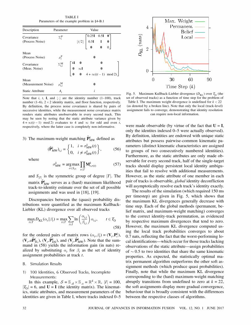
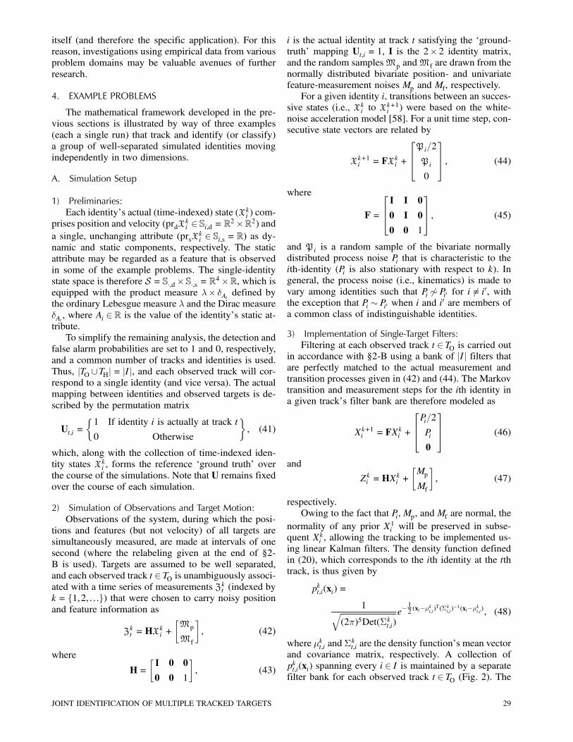
TABLE I

Parameters of the example problem in §4-B.1

Description Parameter Value

Covariance

(Process Noise)

§Pi

bi=2c

240:25I 0:5I 0

0:5I I 0

0 0 0

35Mean

(Process Noise) ¹Pi

0

Covariance

(Meas. Noise)

§Mt,i

244I 0 0

0 1I 0

0 0 4+1((t¡ 1) mod 2)

35Mean

(Measurement Noise) ¹Mt,i 0

Static Attribute Ai i

Note that i, t, I, and b¢c are the identity number (1—100), tracknumber (1—6), 2£ 2 identity matrix, and floor function, respectively.By definition, the process noise covariance is shared by pairs of

successive identities, while the measurement noise covariance matrix

renders static attributes unobservable in every second track. This

may be seen by noting that the static attribute variance given by

4+1((t¡ 1) mod 2) evaluates to 4 and 1 for odd and even t,

respectively, where the latter case is completely non-informative.

3) The maximum-weight matching PkMW defined as

(PkMW)t,i =

½1, i= ¾kMW(t)

0, i 6= ¾kMW(t)

¾, (56)

where¾kMW = argmax

¾2SjTj

Yt2TMkt,¾(t) (57)

and SjTj is the symmetric group of degree jTj. Thematrix PkMW serves as a (hard) maximum likelihood

track-to-identity estimate over the set of all possible

assignments and was used in [18], [19].

Discrepancies between the (quasi) probability dis-

tributions were quantified as the maximum Kullback-

Liebler (KL) divergence over all observed tracks

maxt2T

DKL(®tk¯t) = maxt2T

Xi2Iln

μ®t,i

¯t,i

¶®t,i, t 2 TO

(58)

for the ordered pairs of matrix rows (®t,¯t) = (Vt,Pkt ),

(Vt,aPkTL), (Vt, P

kDS), and (Vt, P

kMW). Note that the sum-

mand in (58) yields the information gain (in nats) re-

alized by substituting ®t for ¯t as the set of identity

assignment probabilities at track t.

B. Simulation Results

1) 100 Identities, 6 Observed Tracks, IncompleteMeasurements:In this example, S = S¢,d£S¢,s = R4£R, jIj= 100,

jTOj= 6, and U= I (the identity matrix). The kinemat-ics, static attributes, and measurement parameters of the

identities are given in Table I, where tracks indexed 0—5

Fig. 5. Maximum Kullback-Liebler divergence (DKL) over TO (the

set of observed tracks) as a function of time step for the problem of

Table I. The maximum weight divergence is undefined for k < 22

(as denoted by a broken line). Note that only the local (track-level)

assignment fails to converge, demonstrating that identity resolution

can require non-local information.

were made observable (by virtue of the fact that U= I,

only the identites indexed 0—5 were actually observed).

By definition, identities are endowed with unique static

attributes but possess pairwise-common kinematic pa-

rameters (distinct kinematic characteristics are assigned

to groups of two consecutively numbered identities).

Furthermore, as the static attributes are only made ob-

servable for every second track, half of the single-target

tracks should display persistent local identity ambigu-

ities that fail to resolve with additional measurements.

However, as the static attribute of one member in each

pair of tracks is observable, global identity deconfliction

will asymptotically resolve each track’s identity exactly.

The results of the simulation (which required 150 ms

per timestep) are given in Fig. 5, which shows that

the maximum KL divergences generally decrease with

time step. Each of the global methods (permanent, be-

lief matrix, and maximum-weight matching) converges

to the correct identity-track permutation, as evidenced

by respective maximum divergences that tend to zero.

However, the maximum KL divergence computed us-

ing the local track probabilities converges to about

0.7 nats, reflecting the fact that the worst-performing lo-

cal identifications–which occur for those tracks lacking

observations of the static attribute–assign probabilities

of » 0:5 to two identities that share the same kinematicproperties. As expected, the statistically optimal ma-

trix permanent algorithm outperforms the other soft as-

signment methods (which produce quasi probabilities).

Finally, note that while the maximum KL divergence

corresponding to the (hard) maximum-weight matching

abruptly transitions from undefined to zero at k = 22,

the soft assignments display more gradual convergence,

behaviour that is broadly consistent with the differences

between the respective classes of algorithms.


TABLE II



Covariance (Process Noise) §Pi

bi=2c

240:25I 0:5I 0

0:5I I 0

0 0 0

35Mean (Process Noise) ¹P

i0

Covariance (Measurement Noise) §Mt,i

244I 0 0

0 1I 0

0 0 4

35Mean (Measurement Noise) ¹M

t,i 0

Static Attribute Ai i

With the exception of the measurement noise covariance, which is

defined in a manner that makes static attribute information visible in

every track, these parameters are identical to those of the first example

(Table I).

2) 100 Identities, 6 Observed Tracks, CompleteMeasurements:This problem is a variation on the previous exam-

ple, differing only by the measurement noise covariance

(Table II), which now extends static attribute visibility

to all observed tracks. In this case, both the local and

global track-to-identity assignments should asymptot-

ically converge to the actual track-to-identity config-

urations. Nonetheless, the global assignments are ex-

pected to exhibit improved pre-asymptotic characteris-

tics, which may be germane to applications that require

interim track-to-identity estimates (or simply do not run

to convergence).

The KL divergences of this simulation (which also

required 150 ms per timestep) are shown in Fig. 6. As

expected, each of the maximumKL divergences tends to

zero with increasing time step. However, between k = 0

and k = 30, there is significant discrepancy between the

local and global identity assignments, supporting the as-

sertion that global identity deconfliction improves target

identification, even when identities are locally resolv-

able. As in the previous example, the permanent-based

algorithm exhibits the fastest soft convergence, and the

maximum-weight matching finds the correct assignment

(in this case for k ¸ 9). Finally, note the significant im-provement in convergence rates as compared to that

of §4-B.1, which may be ascribed to the information

gained from doubling attribute measurements.

3) 100 Identities, 3 Identity Equivalence Classes:In this example, S = S¢,d =R4, jIj= 100, jTOj= 100,

and U= I. No static properties are visible, and iden-

tity dynamics are divided into three equivalence classes

given in Table III (each identity’s Markov process is

described by one of three motion models). The results

of this simulation (which required 270 ms per timestep)

are given in Fig. 7, which shows that global deconflic-

tion significantly improves the resolution of equivalence

TABLE III



Covariance (Process Noise) §Pi i

·0:25I 0:5I

0:5I I

¸Mean (Process Noise) ¹P

i0

Covariance (Measurement Noise) §Mt,i

·4I 0

0 1I

¸Mean (Measurement Noise) ¹M

t,i 0

No. identities in

Equivalence Class 1 n(i = 1) 60

No. identities in


No. identities in


The subscript i indexes the equivalence class. Note the absence of

static attribute information in this example.

Fig. 6. Maximum Kullback-Liebler divergence (DKL) over TO as a

function of time step for the problem of Table II. Once again, the

maximum weight divergence is undefined for k < 9 (as denoted by a

broken line).

class after k » 40. Interestingly, the matrix-permanentalgorithm performs only modestly better than the belief-

matrix method, although both methods significantly

outperform local assignment. Finally, in this example,

convergence of the maximum-weight method appears

substantially more uneven, finding the correct identity-

track assignment at k = 44, then reverting to incorrect

assignments at k = 52 and k = 65 before finally settling

on correct assignment for k ¸ 66.

5. CONCLUSION

This paper derived a rigorously Bayesian method for

finding the optimal track-to-identity assignments for a

group of targets that are well-separated or tracked us-

ing (J)PDA. Identification of targets is performed jointly

across tracks to correctly account for the complex sta-


Fig. 7. Maximum Kullback-Liebler divergence (DKL) over TO as a

function of time step for the problem of Table III. The maximum

weight divergence is undefined for k < 44 and again for k = 52 and

k = 65 (as denoted by broken lines).

tistical dependencies between track-to-identity assign-

ments. The number of tracks need not equal the num-

ber of identities, and arbitrary feature and kinematic

measurements may be used, provided that their cor-

responding sensor models can be characterized statis-

tically. The problem naturally decomposes into local

single-target tracking and classification and global com-

binatorial identity deconfliction, where the former is

based on a unified measure-theoretic framework that

treats tracking and classification on equal footing, and

the latter reduces to computing the permanent of a non-

negative matrix. While the computational complexity

of the matrix permanent poses challenging implemen-

tation issues, Markov chain Monte Carlo methods may

be used to find approximations in polynomial time. Fur-

thermore, the existence of groups of targets that are in-

distinguishable, unobservable, or both allows the Ryser

formula to be modified in a manner that improves com-

putation speed. Reducing the complexity of approximat-

ing non-negative matrix permanents is an area of signif-

icant contemporary research, and advances in this field

will directly benefit the performance of the algorithm

described in this work.

ACKNOWLEDGEMENTS

The author expresses gratitude to D. J. Peters,

G. R. Mellema, A. W. Isenor, and M. Farrell (DRDC,

Atlantic Research Centre) for constructive comments

and discussions during the preparation of this manu-

script.

APPENDIX A MARKOV TRANSITION AND BAYESIANUPDATE

Under conditions 1—5 of §2-B, the Markov transition

step of the general filtering problem (BF.2) may be

expanded as

pXk jZk¡1:1 (x j Zk¡1:1)

=

ZSfXk jXk¡1 (x j x0)pXk¡1jZk¡1:1 (x0 j Zk¡1:1)d¹(x0)

=

ZS

"Yi2I

Xt2Tft,Xk

ijXk¡1i(xi j x0i)

#hCk¡1Dk¡1

¢1Ak¡1 (x)Yi2I

Xt2T(bk¡1t )¡1ak¡1t,i p

k¡1t,i (x

0i)

#d¹(x0):

(59)

Collecting product terms and noting the support of the

ft,XkijXk¡1i(xi j x0i) and pk¡1t,i (xi)–given in (22) and (20),

respectively–yields the simplification

pXk jZk¡1:1 (x j Zk¡1:1) = Ck¡1Dk¡1

¢ 1Ak (x)Yi2I

Xt2T(bk¡1t )¡1ak¡1t,i p

k¡0:5t,i (xi), (60)

where

pk¡0:5t,i (xi) =

Zrk¡1t

fXkijXki(xi j x0i)pk¡1t,i (x

0i)d¹(x

0i) (61)

is the forward-in-time projection of pkt,i(xi). The Bayes-

ian update step may be similarly found by substituting

(20) and (25) into the right-hand side of (BF.1) to

produce

pXk jZk:1 (x j Zk:1)/ fZk jXk (Zk j x)pXk jZk¡1:1 (x j Zk¡1:1)

=

"pkf1Ak (x)

Yi2I(1rkt (xi)(p

kf )¡1gi,Zk (xi)

+1Crkt(xi))

i¢"Ck¡1Dk¡11Ak (x)

Yi2I

Xt2T(bk¡1t )¡1

¢ak¡1t,i pk¡0:5t,i (xi)

i: (62)

Using (21), equation (62) may be rewritten as

pXk jZ1:k (x j Z1:k) =Ck¡1(Dk¡1pkf )1Ak (x)

¢Yi2I

240@ Xt2Tnfo(k)g

(bk¡1t )¡1ak¡1t,i pk¡1t,i (xi)

1A+(bk¡1o(k)p

kf )¡1Ãak¡1o(k),i

Zrko(k)

pk¡0:5o(k),i (x0i)gi,Zk (xi)d¹(x

0i)

!

¢0@ pk¡0:5o(k),i (xi)gi,Zk (xi)R

rko(k)

pk¡0:5o(k),i (x0i)gi,Zk (x

0i)d¹(x

0i)

1A35 : (63)


The terms pkt,i(xi), bkt , and a

kt,i are thus related to their

counterparts at the previous time step by (27) and (28)

for t= o(k) and t 6= o(k), respectively. In particular, notethat only the coefficients associated with the measured

track t= o(k) are updated.

APPENDIX B EVALUATION OF POSTERIORASSIGNMENT PROBABILITIES

A. Track-to-Identity Probabilities as a Ratio ofPermanents

The posterior track-to-identity assignment proba-

bilities Pkt,i are found by integrating the ith-identity

marginalization of state’s joint density function over

over the region of S associated with the tth track. Thismay be expanded with (20) as

Pkt,i =

Zrkt

pXki(x0i)d¹(x

0i)

=

Zrkt

ZSInfig

pXk (x0)d¹(x0i)d¹(x

0SInfig)

=

Zrkt

ZSInfig

CkDk1Ak (x0)

¢Yi02I

Xt02T(bkt0)

¡1akt0,i0pkt0,i0(x

0i0)d¹(x

0): (64)

Noting the decompositions of the indicator function

given in (17) and (18), equation (64) becomes

Pkt,i = CkDk

Zrkt

ZSInfig

X¾2P(I,T)

Yi002I1¾(i00)(x

0i00)

¢Yi02I

Xt02T(bkt0)

¡1akt0,i0pkt,i(x

0i0)d¹(x

0)

= CkDkZrkt

ZSInfig

X¾2P(I,T)

Yi02I

Xt02T(bkt0)

¡1

¢ akt0,i01¾(i0)(x0i)pkt0,i0(x0i0)d¹(x0): (65)

Using (21), this simplifies to

Pkt,i = CkDk

Zrkt

ZSInfig

X¾2P(I,T)

Yi02I(bk¾(i0))

¡1

¢ ak¾(i0),i0pk¾(i0),i0(x0i0)d¹(x0): (66)

As the probability densities in (66) have unit-valued

integrals, integration with respect to xSInfig yields

Pkt,i = CkDk

Zrkt

X¾2P(I,T)

pk¾(i),i(x0i)Yi02I(bk¾(i0))

¡1

¢ ak¾(i0),i0d¹(x0i): (67)

The final integral zeros all terms not indexed by ¾(i) = t,

giving

Pkt,i = CkDk

X¾2P(I,T)¾(i)=t

Yi02I(bk¾(i0))

¡1ak¾(i0),i0 : (68)

The constant Ck may be found by solving

1 =

ZSpX(x

0)d¹(x0)

=

ZSCkDk1Ak (x

0)

¢Yi02I

Xt02T(bkt0)

¡1akt0,i0pkt0,i0(x

0i0)d¹(x

0) (69)

for (Ck)¡1. With the exception of the final integral, thisprocess mirrors the steps of (64)—(68), giving

Ck =DkX

¾2P(I,T)

Yi02I(bk¾(i0))

¡1ak¾(i0),i0 : (70)

Noting that T and I are endowed with total orders,

t 2 T and i 2 I may be used to index the elements ofa jTj £ jIj-dimensional matrix defined as

Akt,i = akt,i: (71)

Similarly, a jTj £ jTj diagonal matrix may be defined as

Bkt,j = diag(bkt ) =

½bkt , t= j

0, t 6= j

¾, (72)

where j has been used in lieu of i, given that i· jIj · jTj(as described in §2-A). Equation (68) thus becomes

Pkt,i = CkDk

X¾2P(I,T)¾(i)=t

Yi02I((Bk)¡1Ak)¾(i0),i0 : (73)

A new jTj £ jTj-dimensional augmented matrix may beconstructed as

[(Bk)¡1Ak j J], (74)

where J is an jTj £ (jTj ¡ jIj)-dimensional matrix ofones. Note that this matrix is empty when jTj ¡ jIj= 0.Reformulated with respect to [(Bk)¡1Ak j J], equation(73) becomes

Pkt,i =CkDk

(jTj ¡ jIj)!X¾2SjTj¾(i)=t

jTjYj=1

[(Bk)¡1Ak j J]¾(j),j , (75)

where SjTj = P(NjTj,NjTj) is the symmetric group of de-gree jTj, and (jTj ¡ jIj)! is the number of terms in SjTjthat are associated with a single term in (the smaller)

P(I,T). Using the second equation in (29) and noting

that Dk may be brought under the sum product by scal-

ing the rows of [BkAk j J] by Bk, equation (69) may berewritten as

Pkt,i =Ck


jTjYj=1

[Ak j BkJ]¾(j),j

=Ck


jTjYj=1

Mk¾(j),j , (76)


where Mk is defined as

Mk = [Ak j BkJ]: (77)

Finally, (76) may be simplified to

Pkt,i =Ck

(jTj ¡ jIj)!Mkt,i

X¾2SjTj¡1

jTj¡1Yj=1

Mk¾(j),j(t; i), (78)

whereMk(t; i) is the matrix formed fromMk by deleting

the tth row and ith column. Equation (70) may be

similarly expressed as

Ck =1

(jTj ¡ jIj)!X¾2SjTj

jTjYj=1

Mk¾(j),j : (79)

Each of the combinatorial sums in (78) and (79) con-

forms to a matrix permanent defined in (32), and

marginal probability in (78) thus becomes the ratio

Pkt,i =Mkt,i

Per(Mk(t; i))

Per(Mk): (80)

While the resulting matrix of marginal probabilities

Pk is at least left stochastic, it becomes doubly stochasticwhen every track is certain to exist, a condition that

results when each identity can be found at some track

and vice versa. In this case, jTj= jIj, J is empty (the btcoefficients are consequently irrelevant), and each track

must therefore exist and correspond to some identity–

regardless of the system’s false alarm probabilities.

When this is undesired, a set of hidden tracks may

be defined in accordance with (1) of §2-A. Finally,

note that groups of identities that are indistinguishable

with respect to the suite of sensors form equivalence

classes, the presence of which is manifested by repeated

columns in Mk.

B. Limiting Process for Zero False-Alarm Probabilities

The zero false-alarm probabilities that were tem-

porarily reassigned non-zero values (Condition 5 in §2-

B) may now be taken to zero in the limit. In what fol-

lows, the pk0·kf inMk of (78) are sequentially brought to

zero for each pk0f for which a limit is required. This pro-

cess commences by recursively expanding (BF.1) and

(BF.2) over all k00 · k with the measurement functiondefined in (24). For any pk

0f undergoing the limiting step,

this yields

limpk0f!0+

pXk jZ1:k (xk0 j Z1:k) =

limpk0f!0+

¢ ¢ ¢ZS1Ak (x

k0)Yi2I

(1rk0t(xk

0i )(p

k0f )¡1gi,Zk0 (x

k0i ) + 1Crk0t

(xk0i ))

¢ ¢ ¢d¹(x1:k¡1), (81)

where 1· k0 · k and the ellipses contain the measure-ment functions for k00 6= k0 and the Markov transitiondensities and their associated integrals for all k00 · k.

Employing the equivalence between (23) and (24) re-

sults in the reformulation

limpk0f!0+

pXk jZ1:k (x j Z1:k) = limpk0f!0+

μ¢ ¢ ¢ZS1Ak0 (x

k0)

¢ÃXi2Ipk

0d,ifZk0 jXk0S (Z

k0 j xk0i )+pk0f

!¢ ¢ ¢d¹(x1:k¡1)

!:

(82)

Noting that the summand in (82) has no dependence on

pk0f , the dominated convergence theorem [60] may be

trivially applied to the constant pk0f term to give

limpk0f!0+

pXk jZ1:k (x j Z1:k) =Ã¢ ¢ ¢ZS1Ak0 (x)

ÃXi2Ipk

0d,ifZk0 jXk0S (Z

k0 j xk0i )

+ limpk0f!0+

pk0f

!¢ ¢ ¢d¹(x1:k¡1)

!

=

Ã¢ ¢ ¢ZS1Ak0 (x)

ÃXi2Ipk

0d,ifZk0 jXk0S (Z

k0 j xk0i )

+0

!¢ ¢ ¢d¹(x1:k¡1)

!, (83)

and the relation

limpk0f!0+

pXk jZ1:k (x j Z1:k) = pXk jZ1:k (x j Z1:k)jpk0f=0 (84)

thus holds. Equation (64) may now be written as

Pkt,ijpk0f=0 =

Zrkt

pXkijZ1:k (xi j Z1:k)jpk0

f=0d¹(xi)

=

Zrkt

limpk0f!0+

pXkijZ1:k (xi j Z1:k)d¹(xi): (85)

As the pXkijZ1:k (xi j Z1:k) may be assumed bounded, and

because the limit in (84) is satisfied pointwise, the dom-

inated convergence theorem may be applied a second

time to yield

Pkt,ijpk0f=0 = lim

pk0f!0+

Zrkt

pXkijZ1:k (xi j Z1:k)d¹(xi): (86)

By way of the algebraic and integration steps between

(64) and (78), the permanent ratio becomes

Pkt,ijpk0f=0 = lim

pk0f!0+

Mkt,i

Per(Mk(t; i))

Per(Mk): (87)

Provided that limpk0f!0+M

k possesses at least one non-

zero permutation, the denominator is positive, and the

limit of (87) may distributed under the permanent oper-

ations through successive applications of the algebraic

limit theorem [61]

Pkt,ijpk0f=0 = ( lim

pk0f!0+

Mkt,i)Per(limpk0

f!0+M

k(t; i))

Per(limpk0f!0+M

k): (88)


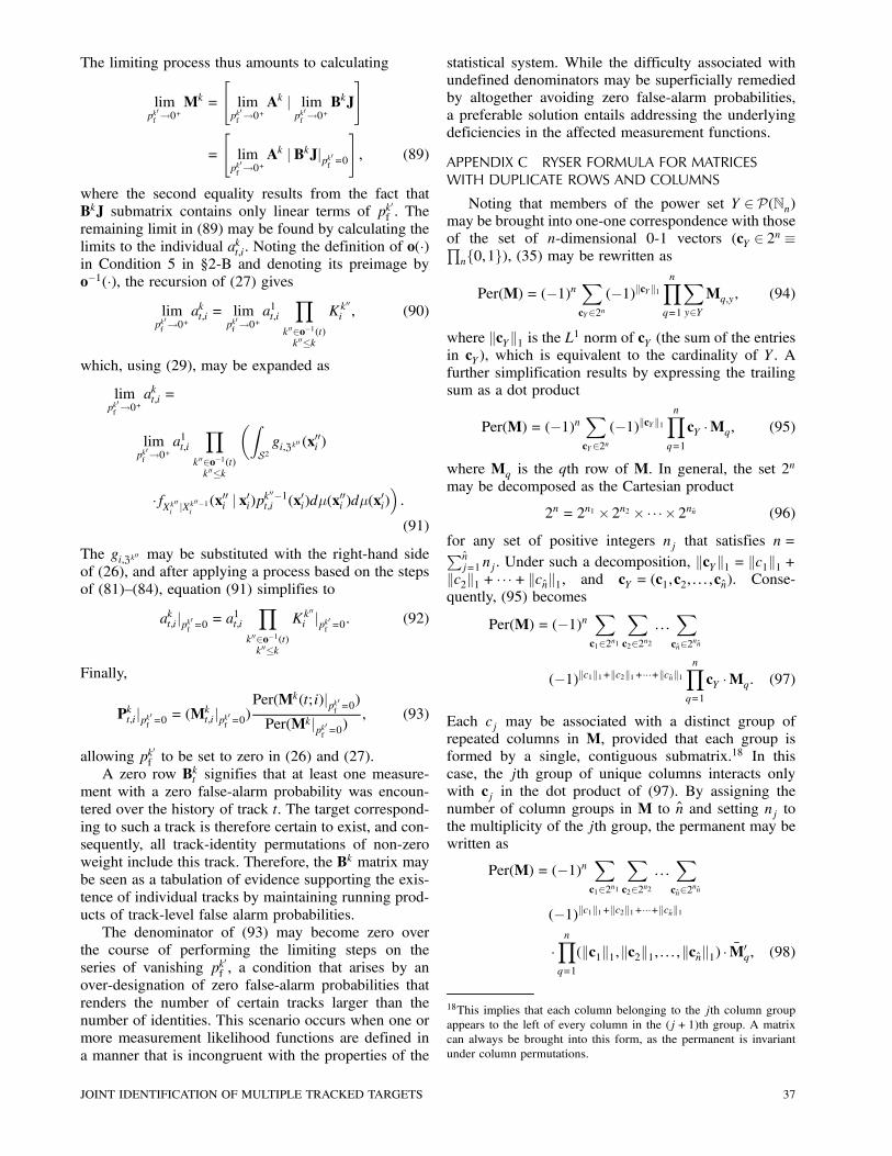
The limiting process thus amounts to calculating

limpk0f!0+

Mk =

"limpk0f!0+

Ak j limpk0f!0+

BkJ

#

=

"limpk0f!0+

Ak j BkJjpk0f=0

#, (89)

where the second equality results from the fact that

BkJ submatrix contains only linear terms of pk0f . The

remaining limit in (89) may be found by calculating the

limits to the individual akt,i. Noting the definition of o(¢)in Condition 5 in §2-B and denoting its preimage by

o¡1(¢), the recursion of (27) giveslimpk0f!0+

akt,i = limpk0f!0+

a1t,i

Yk002o¡1(t)k00·k

Kk00i , (90)

which, using (29), may be expanded as

limpk0f!0+

akt,i =

limpk0f!0+

a1t,i

Yk002o¡1(t)k00·k

μZS2gi,Zk00 (x

00i )

¢fXk

00ijXk00¡1i

(x00i j x0i)pk00¡1t,i (x0i)d¹(x

00i )d¹(x

0i)´:

(91)

The gi,Zk00 may be substituted with the right-hand side

of (26), and after applying a process based on the steps

of (81)—(84), equation (91) simplifies to

akt,ijpk0f=0 = a

1t,i

Yk002o¡1(t)k00·k

Kk00i jpk0

f=0: (92)

Finally,

Pkt,ijpk0f=0 = (M

kt,ijpk0

f=0)Per(Mk(t; i)jpk0

f=0)

Per(Mkjpk0f=0)

, (93)

allowing pk0f to be set to zero in (26) and (27).

A zero row Bkt signifies that at least one measure-

ment with a zero false-alarm probability was encoun-

tered over the history of track t. The target correspond-

ing to such a track is therefore certain to exist, and con-

sequently, all track-identity permutations of non-zero

weight include this track. Therefore, the Bk matrix may

be seen as a tabulation of evidence supporting the exis-

tence of individual tracks by maintaining running prod-

ucts of track-level false alarm probabilities.

The denominator of (93) may become zero over

the course of performing the limiting steps on the

series of vanishing pk0f , a condition that arises by an

over-designation of zero false-alarm probabilities that

renders the number of certain tracks larger than the

number of identities. This scenario occurs when one or

more measurement likelihood functions are defined in

a manner that is incongruent with the properties of the

statistical system. While the difficulty associated with

undefined denominators may be superficially remedied

by altogether avoiding zero false-alarm probabilities,

a preferable solution entails addressing the underlying

deficiencies in the affected measurement functions.

APPENDIX C RYSER FORMULA FOR MATRICESWITH DUPLICATE ROWS AND COLUMNS

Noting that members of the power set Y 2 P(Nn)may be brought into one-one correspondence with those

of the set of n-dimensional 0-1 vectors (cY 2 2n ´Qnf0,1g), (35) may be rewritten as

Per(M) = (¡1)nXcY22n

(¡1)kcYk1nYq=1

Xy2YMq,y, (94)

where kcYk1 is the L1 norm of cY (the sum of the entriesin cY), which is equivalent to the cardinality of Y. A

further simplification results by expressing the trailing

sum as a dot product

Per(M) = (¡1)nXcY22n

(¡1)kcYk1nYq=1

cY ¢Mq, (95)

where Mq is the qth row of M. In general, the set 2n

may be decomposed as the Cartesian product

2n = 2n1 £ 2n2 £ ¢¢ ¢£2nn (96)

for any set of positive integers nj that satisfies n=Pnj=1 nj . Under such a decomposition, kcYk1 = kc1k1 +

kc2k1 + ¢ ¢ ¢+ kcnk1, and cY = (c1,c2, : : : ,cn). Conse-

quently, (95) becomes

Per(M) = (¡1)nXc122n1

Xc222n2

: : :Xcn22nn

(¡1)kc1k1+kc2k1+¢¢¢+kcnk1nYq=1

cY ¢Mq: (97)

Each cj may be associated with a distinct group of

repeated columns in M, provided that each group isformed by a single, contiguous submatrix.18 In this

case, the jth group of unique columns interacts only

with cj in the dot product of (97). By assigning the

number of column groups in M to n and setting nj to

the multiplicity of the jth group, the permanent may be

written as

Per(M) = (¡1)nXc122n1

Xc222n2

: : :Xcn22nn

(¡1)kc1k1+kc2k1+¢¢¢+kcnk1

¢nYq=1

(kc1k1,kc2k1, : : : ,kcnk1) ¢ M0q, (98)

18This implies that each column belonging to the jth column group

appears to the left of every column in the (j+1)th group. A matrix

can always be brought into this form, as the permanent is invariant

under column permutations.


where M0q is the qth row of the smaller matrix M

0, whichcomprises the unique columns of M. As the summands

in (98) depend only on the L1 norm of the cj , the sum

may be rewritten as

Per(M) = (¡1)nn1Xc1=1

μc1n1

¶ n2Xc2=1

μc2n2

¶: : :

nnXc3=1

μcnnn

¶

¢ (¡1)c1+c2+¢¢¢+cnnYq=1

(c1,c2, : : : ,cn) ¢ M0q,

(99)

where the binomial coefficient¡cjnj

¢gives the number

of cj vectors with an L1 norm of cj . Finally, the sums

and binomial coefficients may be collected by defining

d= (c1,c2, : : : ,cn) to give

Per(M) =X

d2QNnj

(¡1)n+kdk124 nYj=1

μdjnj

¶35 nYq=1

d ¢ M0q:

(100)

Inspection of (99)–which is functionally equivalent

to (100)–reveals this reduced form to have a more

favourable complexity of O(nQnj=1(nj +1)) when the

sum are evaluated using a generalized Gray code (i.e.,

consecutive summation terms differ by only a single

dj in d such that (dj +1 mod nj) yields the dj of the

subsequent term).

Finally, when the matrix possess repeated rows, the

dot products d ¢ M0q1and d ¢ M0

q2are equal when q1

and q2 belong to a common row group. The identical

terms may be collected and replaced with a single term

exponentiated to the size of the row group. Equation

(100) then becomes

Per(M) =X

d2QNnj

(¡1)n+kdk1

¢24 nYj=1

μdjnj

¶35 mYq=1

(d ¢ Mq)mq : (101)

where m is the number of unique rows, mq is the size

of the qth group of duplicate rows, and Mq is the qth

row of matrix M comprising only unique rows (and

columns). The time complexity of this simplification is

O(mQj(nj +1)). Finally, as the permanent is invariant

under matrix transposition, the minimum complexity

becomes equation (37).

REFERENCES

[1] S. Challa, M. R. Morelande, D. Mu²sicki, and R. J. Evans

Fundamentals of Object Tracking.

Cambridge: Cambridge University Press, 2011.

[2] S. Challa, R. J. Evans, and D. Musicki

Target Tracking–A Bayesian Perspective,

in Fourteenth International Conference on Digital Signal

Processing, vol. 1. IEEE, 2002, pp. 437—440.

[3] I. R. Goodman, R. P. Mahler, and H. T. Nguyen

Mathematics of Data Fusion.

Dordrecht, The Netherlands: Kluwer Academic Publishers,

1997.

[4] R. E. Kalman

A New Approach to Linear Filtering and Prediction Prob-

lems,

Transactions of the ASME–Journal of Basic Engineering,

vol. 82, no. Series D, pp. 35—45, 1960.

[5] C. K. Chui and G. Chen

Kalman Filtering: With Real-Time Applications.

Springer, 2009.

[6] S. S. Blackman

Multiple-Target Tracking with Radar Applications.

Dedham, MA: Artech House, 1986.

[7] M. Mallick, V. Krishnamurthy, and B.-N. Vo

Integrated Tracking, Classification, and Sensor Management:

Theory and Applications.

Wiley-IEEE Press, 2012.

[8] R. P. Mahler

Statistical Multisource-Multitarget Information Fusion.

Norwood, MA: Artech House, 2007.

[9] B. Ristic, N. Gordon, and A. Bessell

On Target Classification using Kinematic Data,

Information Fusion, vol. 5, no. 1, pp. 15—21, 2004.

[10] M. L. Krieg

Joint Multi-Sensor Kinematic and Attribute Tracking using

Bayesian Belief Networks,

in Proceedings of the 2003 International Conference on

Information Fusion, 2003, pp. 17—24.

[11] –––

“Kinematic and Attribute Fusion Using a Bayesian Belief

Network Framework,”

Defence Science and Technology Organisation, PO Box

1500 Edinburgh, South Australia 5111, Australia, Tech.

Rep., 2006.

[12] W. Mei, G.-l. Shan, and Y.-f. Wang

A second-order uncertainty model for target classification

using kinematic data,

Information Fusion, vol. 12, no. 2, pp. 105—110, 2011.

[13] D. Angelova and L. Mihaylova

Joint Target Tracking and Classification with Particle Filter-

ing and Mixture Kalman Filtering using Kinematic Radar

Information,

Digital Signal Processing, vol. 16, no. 2, pp. 180—204, 2006.

[14] F. Palmieri and D. Ciuonzo

Data Fusion with Entropic Priors,

Proceedings of 20th Workshop on Neural Networks, WIRN,

Frontiers in Artificial Intelligence and Applications, vol. 226,

pp. 107—114, 2011.

[15] J. Teti Jr, R. Gorman, and W. Berger

A Multifeature Decision Space Approach to Radar Target

Identification,

Aerospace and Electronic Systems, IEEE Transactions on,

vol. 32, no. 1, pp. 480—487, 1996.

[16] S. Challa and G. W. Pulford

Joint Target Tracking and Classification Using Radar and

ESM Sensors,

IEEE Transactions on Aerospace and Electronic Systems,

vol. 37, no. 3, pp. 1039—1055, 2001.

[17] B. T. Vo and B. N. Vo

Tracking, Identification, and Classification with Random

Finite Sets,

in SPIE Defense, Security, and Sensing. International Society

for Optics and Photonics, 2013, pp. 87 450D—87 450D.


[18] J. Shin, N. Lee, S. Thrun, and L. Guibas

Lazy Inference on Object Identities in Wireless Sensor

Networks,

in Proceedings of the 4th international symposium on Infor-

mation processing in sensor networks. IEEE Press, 2005,

p. 23.

[19] B. Schumitsch, S. Thrun, G. Bradski, and K. Olukotun

The Information-Form Data Association Filter,

in Advances in Neural Information Processing Systems, 2005,

pp. 1193—1200.

[20] J. Shin, L. J. Guibas, and F. Zhao

A Distributed Algorithm for Managing Multi-Target Iden-

tities in Wireless Ad-Hoc Sensor Networks,

in Information Processing in Sensor Networks. Springer,

2003, pp. 223—238.

[21] H. Balakrishnan, I. Hwang, and C. J. Tomlin

Polynomial Approximation Algorithms for Belief Matrix

Maintenance in Identity Management,

in 43rd IEEE Conference on Decision and Control, vol. 5.

IEEE, 2004, pp. 4874—4879.

[22] I. Hwang, K. Roy, H. Balakrishnan, and C. Tomlin

A Distributed Multiple-Target Identity Management Algo-

rithm in Sensor Networks,

in 43rd IEEE Conference on Decision and Control, vol. 1.

IEEE, 2004, pp. 728—734.

[23] B. Schumitsch, S. Thrun, L. J. Guibas, and K. Olukotun

The Identity Management Kalman Filter (IMKF),

in Robotics: Science and Systems. Citeseer, 2006.

[24] J. Huang, C. Guestrin, and L. Guibas

Fourier theoretic probabilistic inference over permutations,

Journal of Machine Learning Research, vol. 10, pp. 997—

1070, 2009.

[25] –––

Efficient Inference for Distributions on Permutations,

in Advances in Neural Information Processing Systems, 2007,

pp. 697—704.

[26] R. Kondor, A. Howard, and T. Jebara

Multi-Object Tracking with Representations of the Sym-

metric Group,

in International Conference on Artificial Intelligence and

Statistics, 2007, pp. 211—218.

[27] A. S. Asratian

Bipartite Graphs and their Applications.

Cambridge University Press, 1998, no. 131.

[28] R. E. Burkard, M. Dell’Amico, and S. Martello

Assignment Problems, Revised Reprint.

Philadelphia: Society for Industrial and Applied Mathemat-

ics, 2009.

[29] A. B. Badiru and O. A. Omitaomu

Computational Economic Analysis for Engineering and In-

dustry.

Boca Raton, FL: CRC Press, 2010.

[30] M. Fujita and J.-F. Thisse

Economics of Agglomeration: Cities, Industrial Location, and

Globalization.

New York: Cambridge University Press, 2013.

[31] C. K. Mustafi

Operations Research methods and practice.

New Age International, 1996.

[32] H. S. Kasana and K. D. Kumar

Introductory Operations Research: Theory and Applications.

Berlin Heidelberg: Springer-Verlag, 2004.

[33] J. Collins and J. Uhlmann

Efficient Gating in Data Association with Multivariate

Gaussian Distributed States,

IEEE Transactions on Aerospace and Electronic Systems,

vol. 28, no. 3, pp. 909—916, July 1992.

[34] M. Jerrum, A. Sinclair, and E. Vigoda

A Polynomial-Time Approximation Algorithm for the Per-

manent of a Matrix with Non-Negative Entries,

in Proceedings of the Thirty-Third Annual ACM Symposium

on Theory of Computing. ACM, 2001, pp. 712—721.

[35] –––

A Polynomial-Time Approximation Algorithm for the Per-

manent of a Matrix with Nonnegative Entries,

Journal of the ACM (JACM), vol. 51, no. 4, pp. 671—697,

2004.

[36] I. Bezakova, D. ²Stefankovic, V. V. Vazirani, and E. Vigoda

“Approximating the Permanent in O (n7) Time,”

2004.

[37] E. W. Weisstein

CRC Concise Encyclopedia of Mathematics.

Boca Raton, FL: CRC Press, 2003.

[38] L. Hogben

Handbook of Linear Algebra.

Boca Raton, FL: Chapman and Hall/CRC, 2006.

[39] O. Goldreich

Computational Complexity: A Conceptual Perspective.

New York: Cambridge University Press, 2008.

[40] T. Fortmann and Y. Bar-Shalom

Tracking and Data Association.

San Diego: Academic Press, 1988.

[41] L. D. Stone, R. L. Streit, T. L. Corwin, and K. L. Bell

Bayesian Multiple Target Tracking.

Norwood, MA: Artech House, 2013.

[42] T. Granlund

GNU MP, 5th ed., Free Software Foundation, 2013.

[Online]. Available: https://gmplib.org/manual/.

[43] S. Friedland

A Lower Bound for the Permanent of a Doubly Stochastic

Matrix,

Annals of Mathematics, pp. 167—176, 1979.

[44] Lindley, Dennis V

Understanding Uncertainty.

Hoboken, NJ: John Wiley & Sons, 2006.

[45] A. W. Marshall and I. Olkin

Scaling of Matrices to Achieve Specified Row and Column

Sums,

Numerische Mathematik, vol. 12, no. 1, pp. 83—90, 1968.

[46] R. Sinkhorn

A Relationship Between Arbitrary Positive Matrices and

Doubly Stochastic Matrices,

The Annals of Mathematical Statistics, vol. 35, no. 2, pp.

876—879, 1964.

[47] M. Furer

Faster Integer Multiplication,

SIAM Journal on Computing, vol. 39, no. 3, pp. 979—1005,

2009.

[48] B. Kalantari and L. Khachiyan

On the Complexity of Nonnegative-Matrix Scaling,

Linear Algebra and its Applications, vol. 240, pp. 87—103,

1996.

[49] L. G. Valiant

The Complexity of Computing the Permanent,

Theoretical Computer Science, vol. 8, no. 2, pp. 189—201,

1979.

[50] I. Bezakova, D. ²Stefankovi²c, V. V. Vazirani, and E. Vigoda

Accelerating Simulated Annealing for the Permanent and

Combinatorial Counting Problems,

in Proceedings of the Seventeenth Annual ACM-SIAM Sym-

posium on Discrete Algorithms. ACM, 2006, pp. 900—907.

[51] I. Bezakova, D. ²Stefankovic, V. V. Vazirani, and E. Vigoda

Accelerating Simulated Annealing for the Permanent and

Combinatorial Counting Problems,

SIAM Journal on Computing, vol. 37, no. 5, pp. 1429—1454,

2008.


[52] M. Huber and J. Law

Fast Approximation of the Permanent for Very Dense Prob-

lems,

in Proceedings of the Nineteenth Annual ACM-SIAM Sym-

posium on Discrete Algorithms. Society for Industrial and

Applied Mathematics, 2008, pp. 681—689.

[53] B. Huang and T. Jebara

“Approximating the Permanent with Belief Propagation,”

arXiv preprint arXiv:0908.1769, 2009.

[54] P. O. Vontobel

The Bethe Permanent of a Non-Negative Matrix,

in 48th Annual Allerton Conference on Communication, Con-

trol, and Computing. IEEE, 2010, pp. 341—346.

[55] Y. Watanabe and M. Chertkov

Belief Propagation and Loop Calculus for the Permanent

of a Non-Negative Matrix,

Journal of Physics A: Mathematical and Theoretical, vol. 43,

no. 24, p. 242002, 2010.

[56] J. L. Williams and R. A. Lau

“Approximate Evaluation of Marginal Association Proba-

bilities with Belief Propagation,”


Dominic Schaub received his B.Sc. in Computer Engineering and Ph.D. in ElectricalEngineering from the University of Manitoba in 2004 and 2011, respectively. In

2011 he joined Defence Research and Development Canada, Atlantic Research

Centre.

[57] M. Chertkov and A. B. Yedidia

“Computing the Permanent with Belief Propagation,”


[58] Y. Bar-Shalom and X. R. Li

Estimation and Tracking: Principles, Techniques, and Soft-

ware.

Boston: Artech House, 1993.

[59] K. L. Stern

“Hungarian Method C++ Source Code,”

Online, 2012. [Online]. Available: https://github.com/

KevinStern/software-and-algorithms-cpp/blob/master/src/

hungarian.h.

[60] M. Capinski and P. E. Kopp

Measure, Integral and Probability.

London: Springer, 2004.

[61] F. Larusson

Lectures on Real Analysis.

New York: Cambridge University Press, 2012, vol. 21.


CAN UNCLASSIFIED

CAN UNCLASSIFIED

DOCUMENT CONTROL DATA (Security markings for the title, abstract and indexing annotation must be entered when the document is Classified or Designated)

1. ORIGINATOR (The name and address of the organization preparing the document.

Organizations for whom the document was prepared, e.g., Centre sponsoring a

contractor's report, or tasking agency, are entered in Section 8.)

DRDC – Atlantic Research Centre Defence Research and Development Canada 9 Grove Street P.O. Box 1012 Dartmouth, Nova Scotia B2Y 3Z7 Canada

2a. SECURITY MARKING (Overall security marking of the document including

special supplemental markings if applicable.)

CAN UNCLASSIFIED

2b. CONTROLLED GOODS

NON-CONTROLLED GOODS DMC A

3. TITLE (The complete document title as indicated on the title page. Its classification should be indicated by the appropriate abbreviation (S, C or U) in

parentheses after the title.)

Joint Identification of Multiple Tracked Targets

4. AUTHORS (last name, followed by initials – ranks, titles, etc., not to be used)

Schaub, D.E.

5. DATE OF PUBLICATION (Month and year of publication of document.)

September 2017

6a. NO. OF PAGES

(Total containing information,

including Annexes, Appendices,

etc.)

21

6b. NO. OF REFS

(Total cited in document.)

61

7. DESCRIPTIVE NOTES (The category of the document, e.g., technical report, technical note or memorandum. If appropriate, enter the type of report,

e.g., interim, progress, summary, annual or final. Give the inclusive dates when a specific reporting period is covered.)

External Literature (P)

8. SPONSORING ACTIVITY (The name of the department project office or laboratory sponsoring the research and development – include address.)

DRDC – Atlantic Research Centre Defence Research and Development Canada 9 Grove Street P.O. Box 1012 Dartmouth, Nova Scotia B2Y 3Z7 Canada

9a. PROJECT OR GRANT NO. (If appropriate, the applicable research

and development project or grant number under which the document

was written. Please specify whether project or grant.)

9b. CONTRACT NO. (If appropriate, the applicable number under

which the document was written.)

10a. ORIGINATOR’S DOCUMENT NUMBER (The official document

number by which the document is identified by the originating

activity. This number must be unique to this document.)

DRDC-RDDC-2017-P073

10b. OTHER DOCUMENT NO(s). (Any other numbers which may be

assigned this document either by the originator or by the sponsor.)

11a. FUTURE DISTRIBUTION (Any limitations on further dissemination of the document, other than those imposed by security classification.)

Public release

11b. FUTURE DISTRIBUTION OUTSIDE CANADA (Any limitations on further dissemination of the document, other than those imposed by security

classification.)

CAN UNCLASSIFIED

CAN UNCLASSIFIED

12. ABSTRACT (A brief and factual summary of the document. It may also appear elsewhere in the body of the document itself. It is highly desirable that

the abstract of classified documents be unclassified. Each paragraph of the abstract shall begin with an indication of the security classification of the

information in the paragraph (unless the document itself is unclassified) represented as (S), (C), (R), or (U). It is not necessary to include here abstracts in

both official languages unless the text is bilingual.)

This paper derives a rigorously Bayesian technique for estimating the identities of a plurality of

targets that are well separated or tracked using the (joint) probabilistic data association filter. In

contrast to the single-target classification problem, the joint identification of multiple targets is

characterized by statistical dependencies between track-to-identity assignments that render

track-level estimation of identity suboptimal. The present method rigorously accounts for these

dependencies and allows arbitrary feature and kinematic measurements generated by individual

targets to be used in finding the statistically-optimal track-to-identity assignment probabilities.

The problem is decomposed into global combinatorial identity deconfliction and local target

tracking and classification that is based on a unified measure-theoretic filtering framework. The

computational complexity of this technique is shown to be dominated by calculation of the

permanent of a non-negative matrix, which may be found exactly in exponential time or

approximated in polynomial time using Markov chain Monte Carlo methods. Strategies for

improving numerical performance are given for cases where certain subsets of targets are

indistinguishable or unobservable. This work is relevant to applications in tactical settings,

surveillance, including video tracking, air/land/maritime situational awareness, and automated

intelligence collection.

___________________________________________________________________________

13. KEYWORDS, DESCRIPTORS or IDENTIFIERS (Technically meaningful terms or short phrases that characterize a document and could be helpful

in cataloguing the document. They should be selected so that no security classification is required. Identifiers, such as equipment model designation,

trade name, military project code name, geographic location may also be included. If possible keywords should be selected from a published thesaurus,

e.g., Thesaurus of Engineering and Scientific Terms (TEST) and that thesaurus identified. If it is not possible to select indexing terms which are

Unclassified, the classification of each should be indicated as with the title.)

Surveillance; Identity; Tracking; Bayesian; Permanent

Joint Identification of Multiple Tracked...

Documents

Transcript of Joint Identification of Multiple Tracked...