HAL Id: hal-00142629https://hal.archives-ouvertes.fr/hal-00142629

Submitted on 20 Apr 2007

HAL is a multi-disciplinary open accessarchive for the deposit and dissemination of sci-entific research documents, whether they are pub-lished or not. The documents may come fromteaching and research institutions in France orabroad, or from public or private research centers.

L’archive ouverte pluridisciplinaire HAL, estdestinée au dépôt et à la diffusion de documentsscientifiques de niveau recherche, publiés ou non,émanant des établissements d’enseignement et derecherche français ou étrangers, des laboratoirespublics ou privés.

Joint faults detection in LV switchboard and its globaldiagnosis, through a Temperature Monitoring System.

Kahan N’Gouan N’Guessan, Jean-Pierre Rognon, Eric Jouseau, GillesRostaing, Florence François

To cite this version:Kahan N’Gouan N’Guessan, Jean-Pierre Rognon, Eric Jouseau, Gilles Rostaing, Florence François.Joint faults detection in LV switchboard and its global diagnosis, through a Temperature MonitoringSystem.. POWERENG2007, Apr 2007, Setubal, France. pp.736-741. �hal-00142629�

Joint faults detection in LV switchboard and its global diagnosis,

through a Temperature Monitoring System.

Kahan N’guessan (1, 2), Eric Jouseau (2), Jean-Pierre Rognon (1), Gilles Rostaing (1), Florence François (1)

Laboratoire d’Electrotechnique de Grenoble, France (1), Schneider-Electric Services division (2)

E-mail: kahan.n-guessan@schneider-electric.com

Abstract-

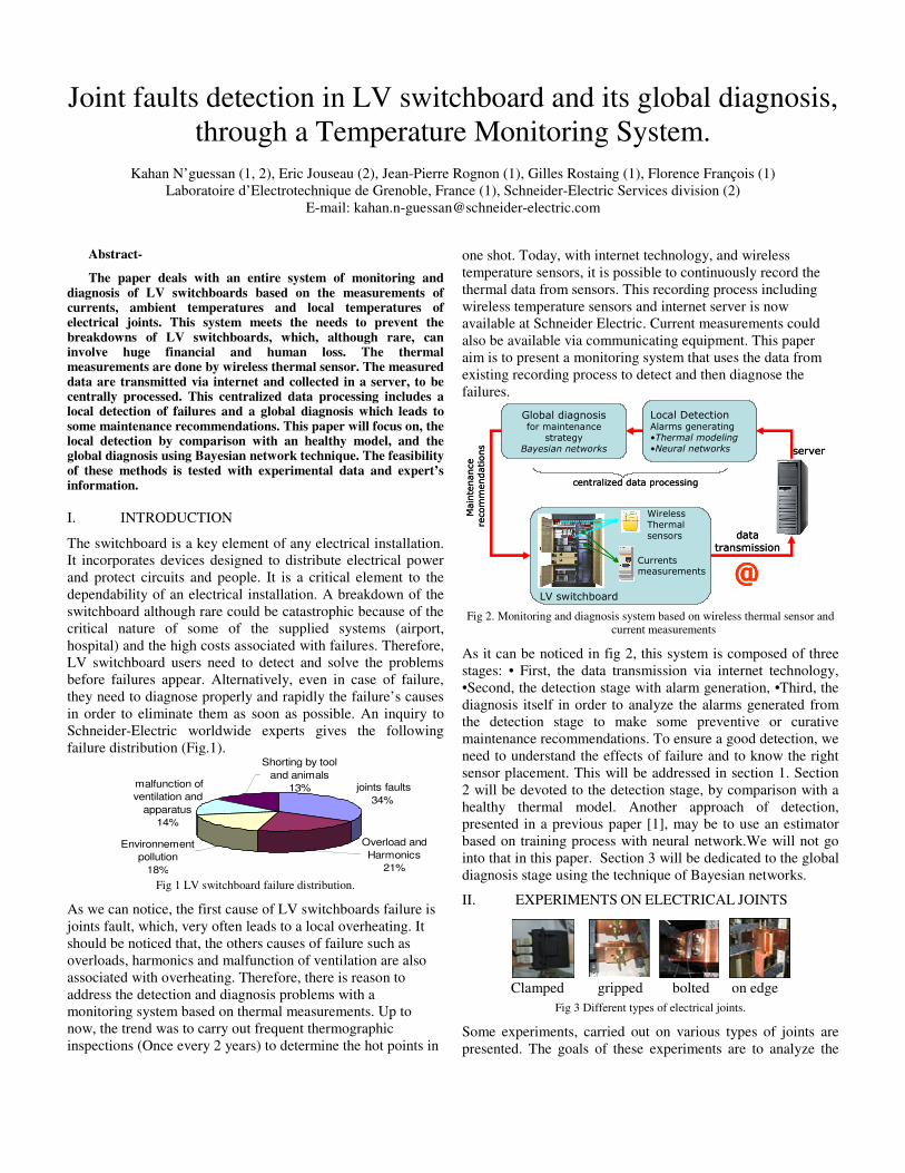
The paper deals with an entire system of monitoring and diagnosis of LV switchboards based on the measurements of currents, ambient temperatures and local temperatures of electrical joints. This system meets the needs to prevent the breakdowns of LV switchboards, which, although rare, can involve huge financial and human loss. The thermal measurements are done by wireless thermal sensor. The measured data are transmitted via internet and collected in a server, to be centrally processed. This centralized data processing includes a local detection of failures and a global diagnosis which leads to some maintenance recommendations. This paper will focus on, the local detection by comparison with an healthy model, and the global diagnosis using Bayesian network technique. The feasibility of these methods is tested with experimental data and expert’s information.

I. INTRODUCTION

The switchboard is a key element of any electrical installation.

It incorporates devices designed to distribute electrical power

and protect circuits and people. It is a critical element to the

dependability of an electrical installation. A breakdown of the

switchboard although rare could be catastrophic because of the

critical nature of some of the supplied systems (airport,

hospital) and the high costs associated with failures. Therefore,

LV switchboard users need to detect and solve the problems

before failures appear. Alternatively, even in case of failure,

they need to diagnose properly and rapidly the failure’s causes

in order to eliminate them as soon as possible. An inquiry to

Schneider-Electric worldwide experts gives the following

failure distribution (Fig.1).

Fig 1 LV switchboard failure distribution.

As we can notice, the first cause of LV switchboards failure is

joints fault, which, very often leads to a local overheating. It

should be noticed that, the others causes of failure such as

overloads, harmonics and malfunction of ventilation are also

associated with overheating. Therefore, there is reason to

address the detection and diagnosis problems with a

monitoring system based on thermal measurements. Up to

now, the trend was to carry out frequent thermographic

inspections (Once every 2 years) to determine the hot points in

one shot. Today, with internet technology, and wireless

temperature sensors, it is possible to continuously record the

thermal data from sensors. This recording process including

wireless temperature sensors and internet server is now

available at Schneider Electric. Current measurements could

also be available via communicating equipment. This paper

aim is to present a monitoring system that uses the data from

existing recording process to detect and then diagnose the

failures.

Fig 2. Monitoring and diagnosis system based on wireless thermal sensor and

current measurements

As it can be noticed in fig 2, this system is composed of three

stages: • First, the data transmission via internet technology,

•Second, the detection stage with alarm generation, •Third, the

diagnosis itself in order to analyze the alarms generated from

the detection stage to make some preventive or curative

maintenance recommendations. To ensure a good detection, we

need to understand the effects of failure and to know the right

sensor placement. This will be addressed in section 1. Section

2 will be devoted to the detection stage, by comparison with a

healthy thermal model. Another approach of detection,

presented in a previous paper [1], may be to use an estimator

based on training process with neural network.We will not go

into that in this paper. Section 3 will be dedicated to the global

diagnosis stage using the technique of Bayesian networks.

II. EXPERIMENTS ON ELECTRICAL JOINTS

Clamped gripped bolted on edge

Fig 3 Different types of electrical joints.

Some experiments, carried out on various types of joints are

presented. The goals of these experiments are to analyze the

data transmission

Wireless Thermal sensors

@

centralized data processing

Currents measurements

Maintenance

recommendations

LV switchboard

Global diagnosisfor maintenance

strategyBayesian networks

Local DetectionAlarms generating •Thermal modeling•Neural networks server

data transmission

Wireless Thermal sensors

@

centralized data processing

Currents measurements

Maintenance

recommendations

LV switchboard

Global diagnosisfor maintenance

strategyBayesian networks

Local DetectionAlarms generating •Thermal modeling•Neural networks server

Shorting by tool

and animals

13%

Environnement

pollution

18%

malfunction of

ventilation and

apparatus

14%

Overload and

Harmonics

21%

joints faults

34%

thermal changes due to joint failures and to find the right

sensors placement. They are related to clamped joint failure

effects, joint progressive loosening, joint aging.

A. Effect of Clamped joint failure.

More and more seen in LV switchboards, clamped joints are

used to connect withdrawable apparatuses, which permit to

drastically reduce the dismantling time during maintenance

operation. The following test has been carried out to illustrate

what happens when a clamped joint fails. The test assembly is

composed of a Schneider Electric three-phase circuit breaker

NS630 installed in a cubicle. We distinguish on fig4 a

clamped joint (with 3 clamps) used to connect each phase of

the circuit breaker. The test will consist of supplying the circuit

breaker with the rated current (520A) in different

configurations, with clamped joints composed of 3 , 2, and 1

clamp respectively. Thermocouples are used to measure the

temperature of selected point numbered from 1 to 13.We can

notice that thermocouples are also placed inside the circuit

breaker. Fig4 gives the resulting profile of temperature in

which we can see that the reduction of the number of clamp

leads to rise the profile of temperature.

Fig 4 Effets of clamped joints failure

This observation could be explained by the increase of the

electrical resistance when reducing the number of clamps (of

each joint). Thus, according to Joule Effect when the current

passes through, the contact becomes the seat of a stronger

creation of heat. The reduction of the number of clamps not

only increases the electrical resistance but the thermal

resistance too[3]. Thus the heat produced by the circuit breaker

has more difficulties to be propagated through the joints. That

results in the noticeable difference in temperature at point 2

and 3 or 11 and 12 in both sides of the “1 clamp” curve. The

conclusion of this experiment for sensor placement is that in

such a configuration, it is preferable to put the sensor on the

side near the circuit breaker. Today, the switchboard

architecture does not always permit this placement. Some

studies are being carried out at Schneider Electric to integrate

the wireless sensor in the clamped joint.

B. Joint progressive loosening

This experiment has been carried out to analyze the

temperature changes generated by a progressive loosening on

three common technologies of electrical joints (gripped joint,

bolted joint, on edge joint).This test consists in supplying a

busbar leading to a joint (gripped, bolted or on edge) with

about the rated current. After the stabilization of the

temperature, progressive loosening of ½, ¼... of the rated

tightening torque is made. The profile of temperature is

measured using thermocouples placed along the busbar (fig5)

Fig 5 Progressive loosening test assembly and results for the gripped joint.

Point 1: Thermocouple placed at 60cm ,Point3; Thermocouple placed at 20cm

Point5:Thermocouple placed on the contac;, Ambient: approximately 50 cm

far from the busbar

The results of the test, for the gripped joint (fig 5), show that it

is necessary to loosen down to less than 1/8 of its rated torque,

(28Nm) to be able to see a significant overheating. This shows

that the electrical resistance of the gripped joint does not vary

enormously during loosening until 4 Nm (around 1/8 of the

rated torque), from which it increases exponentially. Since the

heating results from Joule Effect, heating increases with

electrical resistance[4]. With regard to the other types of joints,

this experiment gives similar results. The on edge joint

distinguishes itself somewhat by greater joint electrical

resistance, more overheating being generated on it (fig 6). The

overheating attenuation can be calculated as the ratio of

overheating on the joint (point 5) to the overheating 200 mm

far from the joint (point 3). Gripped Bolted On edge

Rated torque (RT) 28Nm 50Nm 28Nm

Busbar cross-section(mm²) 80*10 60*10 60*10

Current 1800A 1500A 1500A

Time constant (minutes) 45 40 42

Overheating with 1/4 RT 4°C 3°C 12°C

Attenuation at 20cm 47% 53% 55% Fig 6 Result of progressive loosening test, on the three types of joints.

There is 52% attenuation on average of the overheating on the

three types of joints (gripped, bolted, On edge) at 200 mm

from the joint (point 3).Through the observations made during

this experiment, we can assume that:

To observe a considerable rise in temperature the joint has to

be loosened down 1/8 of the rated torque. Moreover, to detect

the heating effect of the loosening of a joint the sensor has to

be placed less than 200 mm from the joint.

20°C

40°C

60°C

80°C

100°C

120°C

140°C

00:00

00:40

01:20

02:00

02:40

03:20

04:00

04:40

05:20

06:00

06:40

07:20

08:00

Time(h:mn)

Ambiant [°C]

Point 1 [°C]

Point3 [°C]

Point5 [°C]

1/2 1/4 1/8With

hands

31 5

1500

20°C

40°C

60°C

80°C

100°C

120°C

140°C

00:00

00:40

01:20

02:00

02:40

03:20

04:00

04:40

05:20

06:00

06:40

07:20

08:00

Time(h:mn)

Ambiant [°C]

Point 1 [°C]

Point3 [°C]

Point5 [°C]

1/2 1/4 1/8With

hands

20°C

40°C

60°C

80°C

100°C

120°C

140°C

00:00

00:40

01:20

02:00

02:40

03:20

04:00

04:40

05:20

06:00

06:40

07:20

08:00

Time(h:mn)

Ambiant [°C]

Point 1 [°C]

Point3 [°C]

Point5 [°C]

1/2 1/4 1/8With

hands1/21/2 1/41/4 1/81/8

With

hands

With

hands

31 5

150031 531 531 5

1500

80°C

100°C

120°C

140°C

160°C

180°C

200°C

220°C

1 2 3 4 5 6 7 8 9 10 11 12 13

1 clamp

2 clamps

3 clamps

1 2 3 11 134

12

80°C

100°C

120°C

140°C

160°C

180°C

200°C

220°C

1 2 3 4 5 6 7 8 9 10 11 12 13

1 clamp

2 clamps

3 clamps

80°C

100°C

120°C

140°C

160°C

180°C

200°C

220°C

1 2 3 4 5 6 7 8 9 10 11 12 13

1 clamp

2 clamps

3 clamps

1 2 3 11 134

12

inner

5

6 7

8

9 10

5

6 7

8

9 10

C. Joint Aging

In this test, the aging process of the joints is investigated and

then analysis is made of the influence of the current level on

this aging. The test is made on the gripped joint tightened

beforehand at 1/8 of its rated torque to accelerate the aging

process. The experiment consists of supplying the busbar with

cycles of currents. Each cycle consisted of two hours of current

supply followed by a cool-off period of about two and a half

hours. The e-hour duration was chosen to allow the busbar to

reach a stable temperature, after which the busbar was allowed

to cool down to ambient temperature. For the first 12 cycles,

the busbar was supplied with a current of 1800 A, after which

it was supplied with a current of 2200A until cycle 32. Fig 7

gives the temperature rise calculated as the difference of

temperature between point 5 (on the contact) and point 2 (400

mm far from the contact). This curve shows that the number of

cycles affects the joint contact by the rise of the local heating.

Fig 7 Aging test on gripped joint

From cycle 1 to cycle 12, the contact has not aged significantly

From cycle 12 to cycle 32 with a supply current of 2200A

(about 1.5 time of the rated current), a steady increase of the

overheating can be observed. Therefore, the joint indeed ages

in time with the number of cycles. This ageing process is

accelerated by overloads. The ageing process could be

explained by two reasons: The oxidation of the joint interface

metal, which contributes to increase the joint resistance, with

an oxidation speed accelerated by temperature rise due to

overloads. The thermo-mechanical effects involving stress-

relaxation phenomena associated with cycles, which reduces

contact force and consequently increases contact resistance [2].

Through the previous experiments, it is apparent that an

electrical joint holds onto its failure state once the failure

appears, and could get worse under certain conditions. In the

following section, a technique of detection of failures using a

comparison with a healthy model is tested.

III. AUTOMATIC DETECTION OF ABNORMAL

HEATING BY COMPARISON WITH A HEALTHY

THERMAL MODEL.

A. Principle of modeling and automatic detection.

At Schneider Electric, there is an in-house, thermal

computation software based on a representation of the LV

switchboard as a network of nodes connected to each other by

thermal conductance (convective, conductive, and irradiative).

The principle of modeling is a nodal method and the

calculations are done by finite difference. The software takes

into account the electric aspect of the problem through

electrical resistance. This model is suitable for modeling

conduction phenomena, which represents 60 to 70% of heat

exchange phenomena in the switchboard.

Fig 8 Electrical joints’s states estimator.

This software can be used to have a thermal modeling of the

switchboard (Schneider Electric model library). The inputs of

the model are the currents and the ambient temperature of the

switchboard. The output of the model is the temperature on

several selected electrical joints. It should not be forgotten that

most of the time the model result is a bit different from the

experimental results. For reducing the disparity between the

model and the real system, something important to do after

modeling is to make the model in line with an experimental

measurement from a healthy switchboard. This is done by

tuning some parameters as joint electrical resistance, thermal

resistance and heat exchange coefficient. This tuning has to be

done on the operating currents range. Then the fitted model is

used as a reference of a healthy switchboard. Over time, the

drift of the difference from the temperature measured in

comparison with the corresponding temperature from the

model is an estimator of the joints state (fig8). In the following

paragraph we will test this method on a switchboard in real-life

situation.

B. Example of a real switchboard tested and modeled..

: Points of measurement of compartment ambient temperature.

: Busbar with bolted joint. : Clamped joint.

: Compartment. : Points of measurement of joint temperature.

Fig 9 Real LV switchboard in experiment, with associated busbar circuit and measured points.

Currents measurements Thermal image of

the switchboard

ComparisonElectrical joints's state estimator

Temperature Measurements on electrical joints

Ambient temperature measurements

LVSwitchboard

Thermal Modeling•Nodal method•finite difference

Currents measurements Thermal image of

the switchboard

ComparisonElectrical joints's state estimator

Temperature Measurements on electrical joints

Ambient temperature measurements

LVSwitchboard

Thermal Modeling•Nodal method•finite difference

10°C

15°C

20°C25°C

30°C

35°C

40°C

cycle

2

cycle

5

cycle

8

cycle

11

cycle

14

cycle

17

cycle 2

0

cycle

23

cycle

28

cycle 3

1

1800A 2200A

10°C

15°C

20°C25°C

30°C

35°C

40°C

cycle

2

cycle

5

cycle

8

cycle

11

cycle

14

cycle

17

cycle 2

0

cycle

23

cycle

28

cycle 3

1

1800A 2200A

Apparatuses with nominal currents of

3200A and 1600A respectively

Fig 9 shows a real switchboard in the experiment (left), with

one of the three associated busbar circuit phases (right).

Thermocouples have been put on some joints (including bolted

and clamped). Ambient temperatures of selected compartments

have been measured via thermocouples too. First, the

switchboard has been supplied by a current of 1000A the

thermal stabilization occurred after a time period of about four

and a half hours. Fig 10 gives the comparison between

temperatures performed by the modeling software after tuning,

and the real values measured on the joints. It can be noticed on

fig 10 that the temperatures resulting from modeling are very

close to the experimental ones. The average relative error

between the model and the experiment is 1% with a maximum

of 2% on points 2, 4, 6 and 7. To verify the validity of the

model, we choose to supply the switchboard with another

range of current (1600A) in order to make the same

comparison.

35°C

45°C

55°C

65°C

75°C

85°C

95°C

105°C

1 2 3 4 5 6 7 8 9

measured points

Model ExperimentModel Experiment

1600A - checking of the validity

of the model

1000A

Fig 10 Comparison between the model and the experiment after tuning with a

test at 1000A, and validation of the model with a test at 1600A.

The model has been run without changing anything on the

modeling parameters apart from the input current of 1600A.

The graph also gives the comparison between the model and

the experiment with 1600A of supplied current. The average

relative’ error between the model and the experiment is 2%

with a maximum of 4% reached on the point 5. According to

these results, the model can be qualified as valid. Now this

model can be used as a valid reference. In order to check that

the model can detect an abnormal heating, an experiment has

been done with joint 9 loosened at 1/8 of its rated torque. The

supplied current was 1000A. We can see on fig 11 that the

faulty point 9 is abnormally hot, compared to the healthy

model. And the others faultless points are close to the model,

apart from the point 8 a bit affected by the hot temperature on

point 9 through heat exchange.

35°C

40°C

45°C

50°C

55°C

60°C

65°C

1 2 3 4 5 6 7 8 9measured points

Experiment with joint 9 at fault

Healthy Model

Fig 11 Comparison between the model and a test with failure of the joint 9.

IV. DIAGNOSIS OF FAILURES BASED ON

BAYESIAN NETWORKS.

Once the failure has been detected, the following stage should

be the diagnosis itself, that is to know the cause of the failure.

In the present methodology, when a failure occurs, the experts

go on site to seek some indications guiding them to find the

causes of failure. More specifically, knowing the failure, they

seek the indications in a probable family of indications, and

work by an elimination process to find the most likely cause.

Since experts have a probabilistic and inference based

reasoning, one of the natural ways to represent and to automate

this reasoning is by a Bayesian Networks (BN) approach. BN

also allows predictive diagnosis, ie knowledge of consequences

to LV switchboard working conditions, early drift detection.

The second reason in support of the BN choice is that in

numerous industrial diagnosis problems, BN showed

encouraging results [14].

A. Bayesian Network.

It is to the Bayes rule that we owe the term “Bayesian”. BN is

the research results of J.Pearl and a Danish team of Aalbord

University [5]. BN is a causal graph making it possible to bind

a set of effects to their causes. BN combines tables of

conditional probabilities with the causal graph that enables a

probabilistic reasoning on the graph to be accomplished. With

BN it is possible reason in the two directions: the calculations

of the probability of causes knowing the effects but also the

probabilities of the effect knowing the causes. The

implementation of a BN is done in two stages:

• Knowledge acquisition and graph creation.

• Conditional probabilities table (CTP) filling.

Several internal documents in Schneider Electric deal with LV

switchboard failure causes. The reading of these documents

[6]-[7]-[8]-[9] enables us to get an idea of the parameters

acting on the operation of LV switchboard and which could be

useful for its diagnosis. This information has been

supplemented with various discussions with experts. Indeed six

experts were questioned on the possible causes of degradations

of LV switchboards and three among these experts intervened

in the construction and the final validation of the BN. With

regard to BN implementation, we use MATLAB Toolbox,

FullBNT-1.0.2 developed by Kervin Murphy at Berkeley [10].

B. Case of application: Example extracted from the whole graph.

In this section a concrete example of BN is given. This

example is drawn from a complete BN of the LV switchboard.

The choice of this part of the graph was guided by a

preoccupation with simplification. Thus, a part of the graph

with variables that have a reduced number of states was taken.

These variables have been considered as binary. By

considering binary variables, we place ourselves on a level of

diagnosis, which can be interpreted as a "roughing" step in

diagnosis.

1) Information coming from the experts:

• An increase in the external temperature (ET) automatically

involves an increase in the LV switchboard ambient

temperature.• A ventilation obstruction (VO) makes the

circulation of fresh air difficult. Hence, with a VO additional

heating of the internal air of the switchboard is observed. • The

rated current is distributed in the different circuits of the LV

switchboard by taking into account a multiplying factor called

the diversity factor (DF), given by the manufacturer. The

failure to respect this requirement leads to a rise in the internal

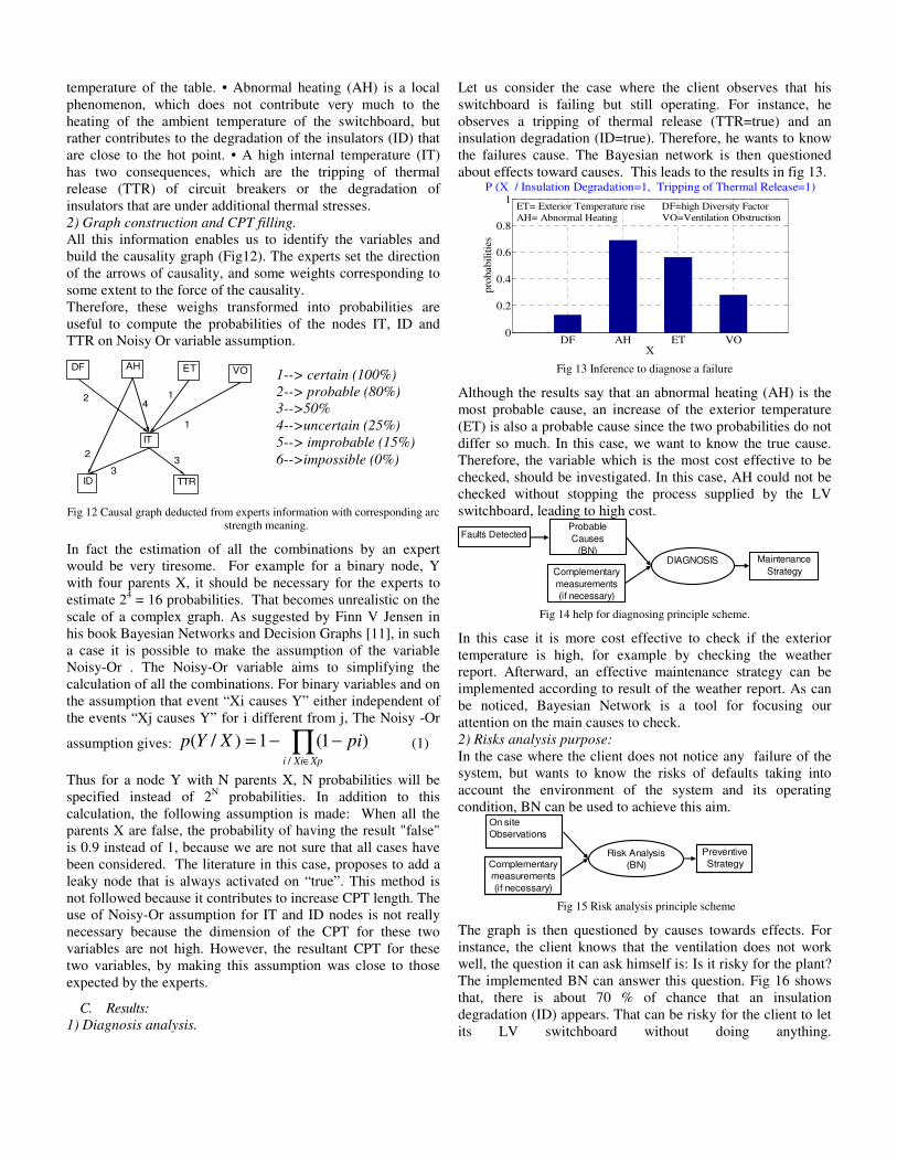
temperature of the table. • Abnormal heating (AH) is a local

phenomenon, which does not contribute very much to the

heating of the ambient temperature of the switchboard, but

rather contributes to the degradation of the insulators (ID) that

are close to the hot point. • A high internal temperature (IT)

has two consequences, which are the tripping of thermal

release (TTR) of circuit breakers or the degradation of

insulators that are under additional thermal stresses.

2) Graph construction and CPT filling.

All this information enables us to identify the variables and

build the causality graph (Fig12). The experts set the direction

of the arrows of causality, and some weights corresponding to

some extent to the force of the causality.

Therefore, these weighs transformed into probabilities are

useful to compute the probabilities of the nodes IT, ID and

TTR on Noisy Or variable assumption.

Fig 12 Causal graph deducted from experts information with corresponding arc strength meaning.

In fact the estimation of all the combinations by an expert

would be very tiresome. For example for a binary node, Y

with four parents X, it should be necessary for the experts to

estimate 24 = 16 probabilities. That becomes unrealistic on the

scale of a complex graph. As suggested by Finn V Jensen in

his book Bayesian Networks and Decision Graphs [11], in such

a case it is possible to make the assumption of the variable

Noisy-Or . The Noisy-Or variable aims to simplifying the

calculation of all the combinations. For binary variables and on

the assumption that event “Xi causes Y” either independent of

the events “Xj causes Y” for i different from j, The Noisy -Or

assumption gives: ∏∈

−−=XpXii

piXYp/

)1(1)/( (1)

Thus for a node Y with N parents X, N probabilities will be

specified instead of 2N probabilities. In addition to this

calculation, the following assumption is made: When all the

parents X are false, the probability of having the result "false"

is 0.9 instead of 1, because we are not sure that all cases have

been considered. The literature in this case, proposes to add a

leaky node that is always activated on “true”. This method is

not followed because it contributes to increase CPT length. The

use of Noisy-Or assumption for IT and ID nodes is not really

necessary because the dimension of the CPT for these two

variables are not high. However, the resultant CPT for these

two variables, by making this assumption was close to those

expected by the experts.

C. Results:

1) Diagnosis analysis.

Let us consider the case where the client observes that his

switchboard is failing but still operating. For instance, he

observes a tripping of thermal release (TTR=true) and an

insulation degradation (ID=true). Therefore, he wants to know

the failures cause. The Bayesian network is then questioned

about effects toward causes. This leads to the results in fig 13.

DF AH ET VO0

0.2

0.4

0.6

0.8

1P (X / Insulation Degradation=1, Tripping of Thermal Release=1)

X

pro

babil

itie

s

ET= Exterior Temperature rise DF=high Diversity Factor

AH= Abnormal Heating VO=Ventilation Obstruction

Fig 13 Inference to diagnose a failure

Although the results say that an abnormal heating (AH) is the

most probable cause, an increase of the exterior temperature

(ET) is also a probable cause since the two probabilities do not

differ so much. In this case, we want to know the true cause.

Therefore, the variable which is the most cost effective to be

checked, should be investigated. In this case, AH could not be

checked without stopping the process supplied by the LV

switchboard, leading to high cost.

Fig 14 help for diagnosing principle scheme.

In this case it is more cost effective to check if the exterior

temperature is high, for example by checking the weather

report. Afterward, an effective maintenance strategy can be

implemented according to result of the weather report. As can

be noticed, Bayesian Network is a tool for focusing our

attention on the main causes to check.

2) Risks analysis purpose:

In the case where the client does not notice any failure of the

system, but wants to know the risks of defaults taking into

account the environment of the system and its operating

condition, BN can be used to achieve this aim.

Fig 15 Risk analysis principle scheme

The graph is then questioned by causes towards effects. For

instance, the client knows that the ventilation does not work

well, the question it can ask himself is: Is it risky for the plant?

The implemented BN can answer this question. Fig 16 shows

that, there is about 70 % of chance that an insulation

degradation (ID) appears. That can be risky for the client to let

its LV switchboard without doing anything.

On site

Observations

Complementary

measurements

(if necessary)

Risk Analysis

(BN)

Preventive

Strategy

Probable

Causes

(BN)

Complementary

measurements

(if necessary)

DIAGNOSIS Maintenance

Strategy

Faults Detected

DF ETAH VO

IT

ID TTR

1

14

2

2

33

1--> certain (100%)

2--> probable (80%)

3-->50%

4-->uncertain (25%)

5--> improbable (15%)

6-->impossible (0%)

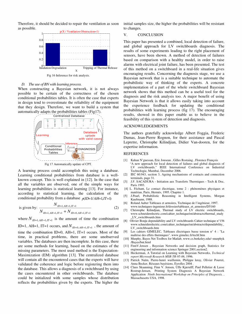
Therefore, it should be decided to repair the ventilation as soon

as possible.

Insulation Degradation Tripping of Thermal Release0

0.2

0.4

0.6

0.8

1p(X / Ventilation Obstruction=1)

X Fig 16 Inference for risk analysis.

D. The use of BN with learning process.

When constructing a Bayesian network, it is not always

possible to be certain of the correctness of the chosen

conditional probabilities tables. It is often the case that experts

in design tend to overestimate the reliability of the equipment

that they design. Therefore, we want to build a system that

automatically adapts the probabilities tables (Fig17).

Fig 17 Automatically update of CPT.

A learning process could accomplish this using a database.

Learning conditional probabilities from database is a well-

known concept. This is well explained in [12]. In the case that

all the variables are observed, one of the simple ways for

learning probabilities is statistical learning [13]. For instance,

according to statistical learning, the calculation of the

conditional probability from a database )1,1/1( === ITAHIDp

is given by:

1,1,01,1,1

1,1,1

======

===

+ ITAHIDITAHID

ITAHID

NN

N (2)

where 1,1,1 === ITAHIDN is the amount of time the combination

ID=1, AH=1, IT=1 occurs, and1,1,0 === ITAHIDN , the amount of

time the combination ID=0, AH=1, IT=1 occurs. Most of the

time, in practical problems, there are some unobserved

variables. The databases are then incomplete. In this case, there

are some methods for learning, based on the estimates of the

missing parameters. The most used method is the Expectation-

Maximization (EM) algorithm [13]. The centralized database

will contain all the encountered cases that the experts will have

validated the coherence and logic before registering them into

the database. This allows a diagnosis of a switchboard by using

the cases encountered in other switchboards. The database

could be initialized with some samples whose distribution

reflects the probabilities given by the experts. The higher the

initial samples size, the higher the probabilities will be resistant

to changes.

V. CONCLUSION

This paper has presented a combined, local detection of failure,

and global approach for LV switchboards diagnosis. The

results of some experiments leading to the right placement of

sensors, have been shown. A method of detection of failures

based on comparison with a healthy model, in order to raise

alarms with electrical joint failure, has been presented. The test

of this method on a switchboard in a real-life situation gives

encouraging results. Concerning the diagnosis stage, we use a

Bayesian network that is a suitable technique to automate the

probabilistic way of thinking of the experts. A concrete

implementation of a part of the whole switchboard Bayesian

network shows that this method can be a useful tool for the

diagnosis and the risk analysis too. A major benefit of using

Bayesian Network is that it allows easily taking into account

the experience feedback for updating the conditional

probabilities with learning process (fig 17). The encouraging

results, showed in this paper enable us to believe in the

feasibility of this system of detection and diagnosis.

ACKNOWLEDGEMENTS

The authors gratefully acknowledge Albert Foggia, Frederic

Dumas, Jean-Pierre Rognon, for their assistance and Pascal

Lepretre, Christophe Kilindjian, Didier Van-dooren, for the

expertise information.

REFERENCES

[1] Kahan N’guessan, Eric Jouseau , Gilles Rostaing , Florence François “A new approach for local detection of failures and global diagnosis of

LV switchboards.” IEEE International Conference on Industrial Technologie, Mumbai, December 2006.

[2] IEC 60.943, section 3, Ageing mechanisms of contacts and connection terminals, page 31.

[3] J.F. SACADURA - Initiation aux Transferts Thermiques - Tech & Doc, Paris 1993.

[4] L. Féchant, Le contact électrique, tome 2 : phénomènes physiques et matériau, Paris, Hermès, 1995. Chapitre 1.

[5] J.Pearl, Probabilistic Reasoning in Intelligent Systems, Morgan Kaufmann, 1988.

[6] Roland Auber Tableaux et armoires, Technique de l’ingénieur, 1997. www.techniques-ingenieur.fr/dossier/tableaux_et_armoires/D5160 [7] Christophe Kilindjian, Thermal study of LV electric switchboards,

www.schneiderelectric.com/cahier_technique/en/abstracts/thermal_study_LV_switchboards.htm

[8] Olivier Bouju dependability and LV switchboards Cahier technique n°156 www.schneiderelectric.com/cahier_technique/en/abstracts/dependability_LV_switchboards.htm

[9] Les cahiers GIMELEC, Tableaux électriques basse tension n° 4 : "La maîtrise des effets thermiques". www.gimelec.fr/techf.htm

[10] Murphy, Bayes Net Toolbox for Matlab, www.cs.berkeley.edu/~murphyk /Bayes/bnt.html [11] FinnV.Jensen , Bayesian Networks and decision graph, Statistics for

engineering and information science Springer 2001,section2. [12] Heckerman, A Tutorial on Learning with Bayesian Networks, Technical

report Microsoft Research MSR-TR-95-06, 1996. [13] Patrick Naïm, Pierre-henri wuillemin, Philippe leray, Olivier Pourret,

Anna Becker, Réseaux bayésiens, Eyrolles 2004 . [14] Claus Skaanning, Finn V. Jensen, Uffe Kjærulff, Paul Pelletier & Lasse

Rostrup-Jensen, Printing System Diagnosis A Bayesian Network Application Ninth International Workshop on Principles of Diagnosis, , Massachusetts USA, 1998.

Conditional

Probabilities

Tables

DIAGNOSIS

LearningDatabase

uptade

with valid cases

Inference

Centralized Database