AVO analysis

CREWES Research Report — Volume 9 (1997) 34-1

Joint AVO analysis of PP and PS seismic data

Yong Xu and John C. Bancroft

ABSTRACT

This paper makes efforts to explore joint-analyzing the amplitude versus offsetphenomena in the PP and PS data with expectation to reduce the ambiguity of AVOanalysis by utilizing the redundancy of multi-component AVO measurements. Theconvenient approximations of P-P and P-S reflection coefficient are obtained, whichlink the seismic data with the elastic parameters that are sensitive to the hydrocarbonexisting in the rock. A great deal of model and real data is used to test the methods.

In this paper, we derive the approximation of PS reflection coefficient fromZoeppritz equation, correct Aki and Richards’s approximation, and derive someequations of PS reflection coefficient possibly easy to be used in PS AVO analysis.

We study the laboratory and well logging results, and show the difference betweenbulk modulus (κ) and rigidity or shear modulus (µ) is influenced by fluid-fill morepurely, and it is a sensitive and quantitative indicator of gas existing.

P-P and P-S reflection coefficient equations are expressed with the elasticparameters (λ and µ, or κ and µ) in the paper. And it is shown by the well log thatthis kind of expression magnify the changes embedded in the Vp and is advantageousto extract the anomaly caused by fluid-fill.

The method to extract the zero offset section or approximate normal incidencesection is present in the paper. The method in this paper is based on the PP reflectioncoefficient with only care on constant term independent of incident angles.

Wells and 10 Hz vertical component seismic data from Blackfoot, Alberta areused to test our methods and theory. We amplitude-preserved process verticalcomponent data, and extract the elastic parameters and zero offset. We are workingon the radial component data set and hope the elastic parameter extraction from radialcomponent may support the extraction from vertical component data set.

INTRODUCTION

Amplitude versus offset relationships can be considered from a theoretical orpractical standpoint. In theory, as the AVO phenomena translates the sharing of theenergy of the incident compressible wave between the compressible and convertedreflections, the observation of the converted mode AVO would be redundant. Inpractice, a few years of experience in P-mode AVO observation may lead to differentconclusions. In some privileged areas, the AVO of compressible waves effectivelyprovides the expected information. In most cases, single fold data are not pureenough to provide reliable amplitude measurements, and finally the result is doubtful.In such cases, study of the AVO of the converted mode can be advantageous: when

Xu and Bancroft

34-2 CREWES Research Report — Volume 9 (1997)

compatible with the P-P AVO, it confirms it, and when not, it denounces unreliableinformation.

The Zoeppritz equations describe the reflections of incident, reflected, andtransmitted P waves and S waves on both sides of an interface. For analysis of wavereflection we need an equation which relates reflected wave amplitudes to incidentwave amplitudes as a function of angles of incidence. In the past decade, many formsof simplifications of Zoeppritz equation of P-P reflection coefficient appeared in theliterature and industrial practice (Aki and Richards, 1980, Shuey, 1985, Parson, 1986,Smith and Gidlow, 1989, Verm and Hilterman, 1994). Each of these simplificationsin a degree links reflection amplitude with variations of rock properties. Aki andRichard (1980) give the approximation of P-S reflection coefficient. There is also arough approximation linking P-S reflection coefficient with pure SH reflectioncoefficient (Frasier and Winterstein, 1993, Stewart, 1995). Because of the challengesin the processing of the real radial data which are mainly P-S reflections, applicationsof P-S reflection coefficient and AVO analysis rarely appear in the literatures andpractice. We would like to have a PS reflection coefficient equation accurate and easyto link seismic with rock property changes. In this paper, we derive theapproximation of PS reflection coefficient from Zoeppritz equation, corrected Akiand Richards’s approximation for great S wave property changes, and derive someforms of PS reflection coefficient equations possibly easy to be used in P-S AVOanalysis.

In AVO analysis, practices mainly focus on looking for more sensitive indicator ofhydrocarbon and extracting and exploiting anomalous variations between seismic andthese sensitive parameters. Some authors (Goodway et al 1997) showed theadvantages of converting velocity measurements to Lame’s moduli parameters (λ andµ) to improve identification indicator of reservoir zones. Castagna et al (1985)observed a few relationships of compressible wave and shear wave in the clasticsilicate rocks. These give us good empirical guidance to study the rock property fromseismic data. We study these relationships and well logging data, and show thedifference between bulk modulus and rigidity is a sensitive and quantitative indicatorof gas existing.

Least square regression analysis and inversion are the common approaches in theAVO analysis. Parson (1986) obtained contrasts of three elastic parameters (λ, µ, andρ) by pre-stack inversion. Goodway et al (1997) obtained the Vp and Vs frominversion and converted them to the λ/µ to detect the reservoirs. However, thenonuniqueness is always the problem in the seismic inversion. The backgroundvelocity error causes the ratio to change greatly or eliminates the high frequencycontrast. Appropriate selection of parameters, background velocity, waveletestimation, application of a priori information are still important issues which remainto be resolved. Here we choose the least square regression analysis to extract elasticparameters from pre-stack data. The extraction provides band-limited information onwhich we attempt to discover anomaly caused by hydrocarbon reservoirs. And wealso invert the band-limited result by recursive inversion and model-based inversion.In the regression analysis, we express the P-P and P-S reflection coefficient equations

AVO analysis

CREWES Research Report — Volume 9 (1997) 34-3

with the elastic parameters (λ and µ, or κ and µ) and extract these parameters directlywithout conversion from velocity.

Because of drawbacks in seismic methods such as the band-limited feature andnoise level, we are always trying to obtain information from different approaches andinterpret it comprehensively. The zero offset section obtained by linear regression ofpre-stack data provides a better approximation to the normal incidence P-wavereflection coefficient and broader bandwidth and higher resolution. The values oftriangular functions of incident and reflected angles are usually necessary in AVOparameter extraction from seismic data. However, the big errors of obtaining intervalvelocity from rms velocity and computation costs of ray tracing are raised. Themethod in this paper is based on the P-P reflection coefficient with only care onconstant term independent of incident angles. The analysis can be done in t-x or f-xdomains without computation of ray parameters or incident angles.

Multi-component data were acquired from Blackfoot, Alberta. In this paper, wellsand 10 Hz vertical component seismic data are used to test our methods. In thispaper, the difficulties in the P-S data processing are discussed. We are working on theradial component data processing. The results will hopefully be shown soon.

APPROXIMATION OF P-S REFLECTION COEFFICIENT

Approximations of the Zoeppritz equations

In c id e n t P

r e f le c t e d P

r e f le c t e d S

t r a n s m it t e d Pt r a n s m it t e d S

i 1

i 2

j 1

j 2

i 1

ρ1 α 1 β1

ρ2 α 2 β2

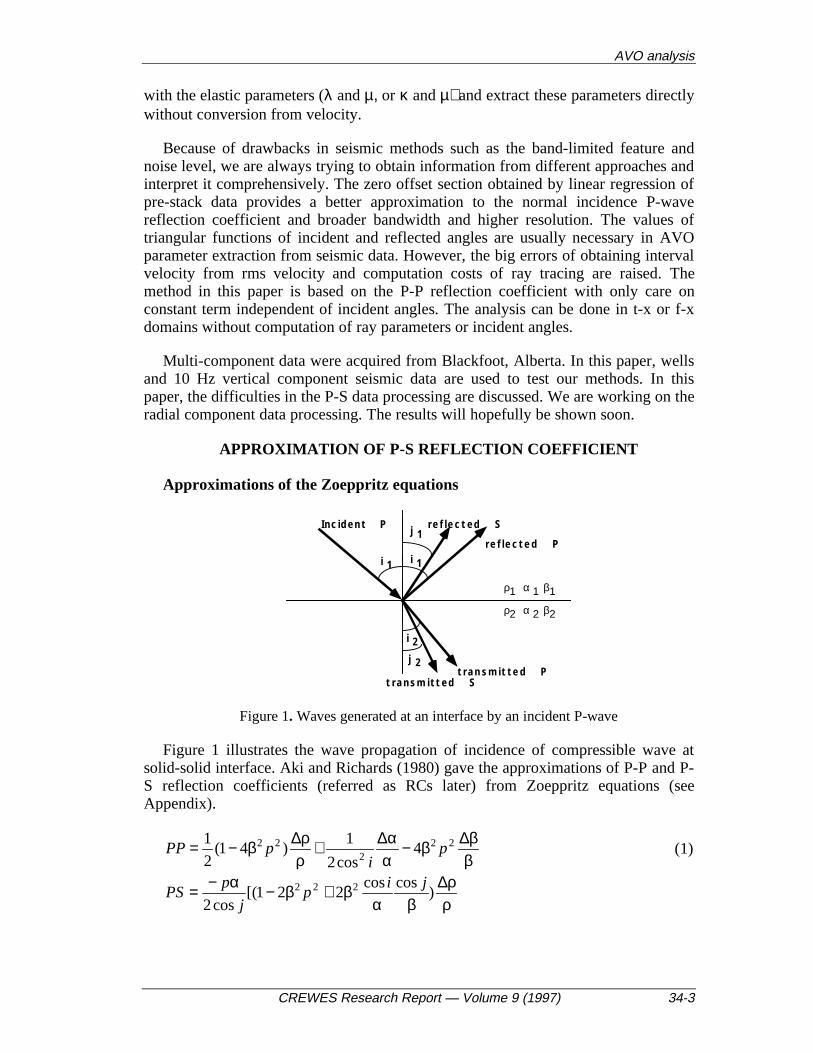
Figure 1. Waves generated at an interface by an incident P-wave

Figure 1 illustrates the wave propagation of incidence of compressible wave atsolid-solid interface. Aki and Richards (1980) gave the approximations of P-P and P-S reflection coefficients (referred as RCs later) from Zoeppritz equations (seeAppendix).

ββ∆β−

αα∆+

ρρ∆β−= 22

222 4

cos2

1)41(

2

1p

ipPP (1)

ρρ∆

βαβ+β−α−= )

coscos221[(

cos2222 ji

pj

pPS

Xu and Bancroft

34-4 CREWES Research Report — Volume 9 (1997)

])coscos

44( 222

ββ∆

βαβ−β− ji

p (2)

The elastic properties in above equations are related as follows to those on eachside of the interface:

)( 12 α−α=α∆ , 2/)( 12 α+α=α , (3)

)( 12 β−β=β∆ , 2/)( 12 β+β=β , (4)

and

)( 12 ρ−ρ=ρ∆ , 2/)( 12 ρ+ρ=ρ . (5)

The angle i is the average of incident and transmitted P-wave angles while j is theaverage of reflected and transmitted S-wave angles:

2/)( 21 iii += and 2/)( 21 jjj += . (6)

Accuracy of P-S RC approximations

Ostrander (1984) devised a hypothetical gas sand model to analyze plane-wavereflection coefficients as a function of angle of incidence. Figure 2 shows Ostrander’smodel, a three layer gas sand model with parameters which might be typical for ashallow, young geologic section. Here, gas sand with a Poisson’s ratio of 0.1 isembedded in shale having a Poisson’s ratio of 0.4. There is a 20 percent P-wavevelocity reduction going into the sand, from 10,000 ft/s to 8,000 ft/s, and a 10 percentdensity reduction from 2.40 g/cm3 to 2.14 g/cm3. The Poisson’s ratio is changed to0.4 if there is no gas in the sand layer. This would simulate the case of low-velocitybrine-saturated young sandstone embedded in shale.

S H A L E

S H A L E

G A SS A N D

V p 1 = 1 0 , 0 0 0ρ 1=2.40σ 1 = 0 .4

V p 3 = 1 0 , 0 0 0ρ3 =2.40σ 3 = 0 .4

V p 2 = 8 , 0 0 0ρ2 =2.14σ 2 = 0 .1

Figure 2. Three-layer hypothetical gas sand model (Ostrander, 1984)

AVO analysis

CREWES Research Report — Volume 9 (1997) 34-5

(a) (b)

Figure 3. The exact and approximated reflection coefficients in the media with elasticproperties specified in Figure 2.

In Figure 3, the exact and approximated reflection coefficients are compared in themedia with elastic properties specified in Figure 2. The solid lines are for the exactand the dash lines are for Aki-Richards approximations. Here, the cases without gasin the sand of second layer in Figure 2 are shown also, in which the Poisson ratio isof 0.4. Panel (a) shows P-P reflection coefficients for the two interfaces in Figure 2and for two cases--with and without gas in the sand. Panel (b) shows P-S reflectioncoefficients for the two interfaces in Figure 2 and for two cases--with and without gasin the sand. After comparing panel (a) and panel (b), we observe three points:

• At normal incidence on the interface with elastic property variation, P-Sreflection coefficient is zero and P-P reflection coefficient is not zero.

• In the small incident angle case, the magnitude of P-P reflection coefficient isbigger than magnitude of P-S reflection coefficient.

• Aki-Richards approximation of P-S reflection coefficient, equation (2) hasbigger relative error than the approximation of P-P reflection coefficient,equation (1) in the model cases in Figure 2, especially the gas-filled sandcases. It is necessary to correct the Aki-Richards approximation of P-Sreflection coefficient.

Under the definitions (3), (4), (5) and (6) with truncation after

,,,,)(,)( 22

ρρ∆

ββ∆

ρρ∆

αα∆

ββ∆

αα∆

ββ∆

αα∆

and 2)( ρρ∆

, after expanding the exact

reflection coefficient from Zoeppritz equations (see Appendix), the higher orderapproximations for P-S reflection coefficient should be:

Xu and Bancroft

34-6 CREWES Research Report — Volume 9 (1997)

])()()(

)()([

2543

22

121

ββ∆+

ββ∆

αα∆+

ββ∆

ρρ∆+

αα∆

ρρ∆+

ρρ∆+

ββ∆+

ρρ∆=

DDD

DDCCAPS

(7)

where

j

iA

cos

sin

2

1−= ,

jijC coscos2sin21 21 α

β+−= ,

)coscos4sin4( 22 jijC

αβ−−= ,

)cos(sin4coscossin32

1 221 jijjijD −

αβ−

αβ−−= ,

jijiD coscos2costan2

1 22 α

β−= ,

jjj

ijijD 222

3 sin7)cos1(cos

cos)cos(sin16

2

1 −+αβ−−

αβ+= ,

jijiD coscos2sintan2 224 α

β−−= ,

and

D5 = 5sin2 j .

The accuracy of equation (7) are compared with the accuracies of Zoeppritzequation, and Aki-Richards approximation--equation (2) in Figure 4, in which thereflection coefficients and relative errors of approximations versus incident angle areplotted. In Figure 4, the later equation (12) and equation (13) are also plotted.

Aki-Richards approximation--equation (2) can be rewritten as polynomial ofcos(i+j) or sin2j as equation (8) and equation (9).

PS = A[P0 + P1 cos(i + j)] (8)

where

AVO analysis

CREWES Research Report — Volume 9 (1997) 34-7

jj

iA tan

2

1

cos2

sin

βα−=−= ,

P0 =

∆ρρ

, BPαβ= 21 , and

ββ∆+

ρρ∆= 2 B .

With Snell’s law and truncation after sin6j, equation (8) is expanded as:

PS = A[C0 + C1 sin2 j + C2 sin 4 j] (9)

where

BCαβ+

ρρ∆= 20 , 2

1 )1( +βα

αβ−= BC , and 2

2

2

2 )1(4

1 +βα

αβ−= BC .

Further approximation of equation (9) by dropping the sin4j term is the followingequation (10), and its accuracy is as good as that of equation (9) for the small andintermediate incident angles.

PS = A(C0 + C1 sin2 j) (10)

Expand A in term of sinj, then we have:

PS = D1 sin j + D2 sin3 j (11)

where

01 2

1CD

βα−= , and )

2

1(

2

1102 CCD +

βα−= .

From comparisons of the curves in Figure 4, we find that the Aki-Richardsapproximations of P-S reflection coefficient as equation (2) or equation (8) are notaccurate enough. Figure 5 compares equation (2), equation (7) after divided by tanj,and we find the error of Aki-Richards approximation is great in the near normalincidence. Using equation (7), we can correct equation (8) and equation (9). If only P0

in equation (8) and C0 in equation (9) are corrected, the approximations could bemore accurate than equation (2)--the Aki-Richards approximation. Equation (12) andequation (13) as follows are the corrected formulas:

PS = A[P0 + P1 cos(i + j)] (12)

where

jj

iA tan

2

1

cos2

sin

βα−=−= ,

ppss BRRPαβ−+

ρρ∆= 2)1(0 ,

Xu and Bancroft

34-8 CREWES Research Report — Volume 9 (1997)

BPαβ= 21 ,

)(2

1

ββ∆+

ρρ∆=ssR ,

Rpp =

1

2(∆ρρ

+∆αα

) ,

and

.22 ββ∆+=

ββ∆+

ρρ∆= ssRB

PS = A[C0 + C1 sin2 j + C2 sin 4 j] (13)

where

)1(2)1(0 ppss RBRC −αβ++

ρρ∆= ,

21 )1( +

βα

αβ−= BC , and 2

2

2

2 )1(4

1 +βα

αβ−= BC .

In Figure 4 and Figure 5, equation (12) and equation (13) are compared with Aki-Richards approximation, equation (7) and the exact.

(a) (b)

AVO analysis

CREWES Research Report — Volume 9 (1997) 34-9

(c) (d)

(e) (f)

(g) (h)

Figure 4. Comparisons of the exact P-S reflection coefficients, Aki-Richardsapproximation (2), equation (7), equation (12) and equation (13) for the three-layer sandmodel in Figure 2. (a), (b), (c), and (d) are the reflection coefficients versus incident angles.(e), (f), (g), and (h) are the relative errors versus incident angles.

Xu and Bancroft

34-10 CREWES Research Report — Volume 9 (1997)

(a) (b)

(c) (d)

Figure 5. Plots of equations (2), (7), (12) and (13) after divided by tanj versus incidentangle.

The model used in Figure 2 is a young gas sand model with big S wave propertychange at the interface. Now investigate another gas sand model with properties ofoverburden shale and gas sand in Table 1. This model is common case to generate theP-P AVO anomaly and may be classified as Class III (Rutherford and Williams,1989).

Table 1 Property of second gas sand model.

Vp Vs Density

Shale 3811 2263 2.40

Gas sand 3453 2302 2.10

Figure 6 shows the comparison of approximations and exact reflection coefficientsfor this model in Table 1. The Aki-Richards’ approximation is good enough for thismodel in which shear wave velocities have smaller changes.

AVO analysis

CREWES Research Report — Volume 9 (1997) 34-11

(a) P-S reflection coefficients (b) enlargement of part of (a)

Figure 6. Comparison of approximation and exact reflection coefficients for gas sandmodel in Table 1.

The average relative errors of Aki-Richards’ approximation for P-S reflectioncoefficients on the interfaces of the macro layers extracted from 08-08 well inBlackfoot survey (Figure 7) are calculated. The incident angle range is 1-40 degrees.Except the top of Mississippian, most of the relative error is less than 10% (Thebiggest is 7.5%).

After tested by different models, the Aki-Richards approximation of P-S reflectioncoefficient can be regarded good for the small incident angles and small S waveproperty changes. The error of this approximation would be tolerant for a great partof cases in the real world.

Figure 7. The average relative error of macro layers from well logs (Blackfoot 0808 well).

Xu and Bancroft

34-12 CREWES Research Report — Volume 9 (1997)

Relationship between PS and SS

Stewart (1995) showed an approximate relationship between converted-wavereflectivity PS and pure SH reflectivity SS. The equation that approximates the pureSH reflectivity is given (Aki and Richards, 1980) as:

ββ∆β−−

ρρ∆β−−= )4

cos2

1()41(

2

1 222

22 pj

pSS (14)

The relationship between converted-wave reflectivity PS and pure S reflectivity SSis as:

])21(8[cos2 ρ

ρ∆αβ−+

αβ−α−= SS

j

pPS (15)

Now as 2

1~

αβ

, the second term in the equation (15) is very small. Thus

PS ~ 4sinj SS0 (16)

Where

)(2

10 β

β∆+ρρ∆−=SS

With the hypothetical model in Figure 2, the exact P-S reflection coefficients,Aki-Richards approximations, and higher order approximation--equation (7) andequation (15) are compared. Figure 8 shows comparisons of the P-S reflectioncoefficients of equation (2), (7), and (15) as a function of incident angle. And the gassand model in Table 1 is also used to test the equation (15) and the comparison isshown in Figure 9.

(a) (b)

AVO analysis

CREWES Research Report — Volume 9 (1997) 34-13

(c) (d)

Figure 8. Comparisons of P-S reflection coefficients in equation (7), Aki-Richardsapproximation—equation (2), equation (7), and equation (15) --relationship between PS andSS. The four panels are the P-S reflection coefficients versus angle of incidence for the three-layer sand model in Figure 2.

(a) Reflection coefficients (b) enlargement of part of (a)

Figure 9. Comparison of approximation and exact reflection coefficients for gas sandmodel in Table 1.

κ−µ AS DIRECT HYDROCARBON INDICATOR

Stewart (1995) advised that λ/µ might have less influence of lithology andhighlight pore-fill changes. Goodway et al. (1997) observed the conversion fromvelocity measurements to Lame’s moduli parameters of rigidity (µ) andincompressibility (λ) improves identification of reservoir zones. And cases show themoduli ratio of λ/µ is a sensitive hydrocarbon indicator. In the following, we alsodiscuss the hydrocarbon indication of elastic parameters—κ,λ, and µ, and observesome interesting points.

Xu and Bancroft

34-14 CREWES Research Report — Volume 9 (1997)

Dry rock line

Castagna et al. (1985) showed the relationships between compressible-wave andshear-wave velocities in clastic silicate rocks. Here some points are quoted:

(1) Gassmann’s equations are

Q

Q

S

DSW +κ

+κκ=κ , (17a)

)(

)(

FS

DSFQκ−κφκ−κκ

= , (17b)

DW µ=µ , (17c)

and

SFW ρφ−+φρ=ρ )1( , (17d)

where κW is the bulk modulus of the wet rock, κS is the bulk modulus of the grains,κD is the bulk modulus of the dry frame, κF is the bulk modulus of the fluid, µW is theshear modulus of the wet rock, µD is the shear modulus of the dry rock, ρW is thedensity of the wet rock, ρF is the density of the fluid, ρS is the density of the grains,and φ is the porosity.

(2) As in Figure 10 (a), the dry line established with laboratory data (Vp/Vs > 1.5)means that dry bulk modulus (κD) is approximately equal to dry rigidity (µD)

DD κ≈µ (18)

These are exactly equal when

53.1/ =DS

DP VV (19)

From equation (17c) it follows that

WDD µ=µ≈κ (20)

The Poisson’s ratio is close to 0.1 in the dry rock and independent of P wavevelocity (see Figure 10 b).

(3) Water saturation causes the bulk modulus to increase. This effect is mostpronounced at higher porosities (lower moduli). Water-saturated bulk modulusnormalized by density is linearly related to compressible velocity (see Figure 10 (c)).

AVO analysis

CREWES Research Report — Volume 9 (1997) 34-15

(a) (b)

(c) (d)

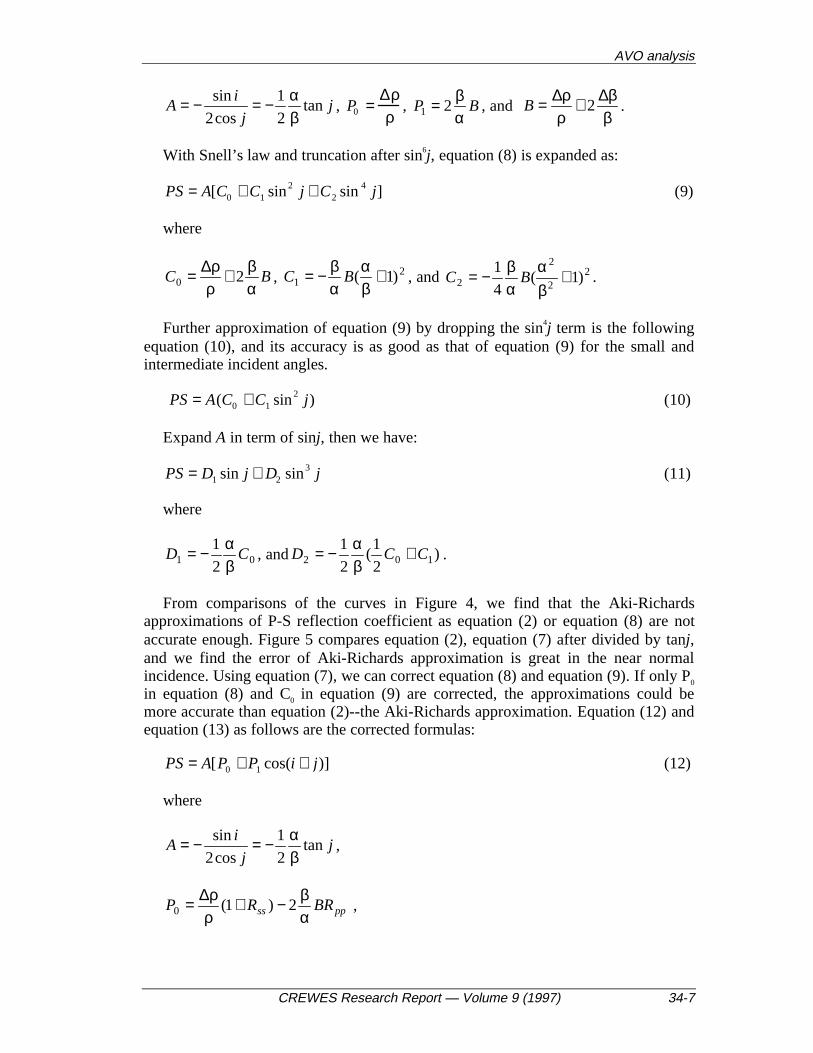
Figure 10. Relationships of clastic rocks (Castagna, 1985). (a) The computedrelationships between the bulk and shear moduli (normalized by density) based on theobserved Vs and Vp trends. (b) The computed relationships between Poisson’s ratio and Vpbased on the observed Vs and Vp trends. (c) The computed relationships between the bulkmodulus (normalized by density) and Vp based on the observed Vs and Vp trends. (d)Gassmann’s equation prediction and observed Vp and Vs.

κ−µ as direct hydrocarbon indicator

Compared with the grain bulk modulus and frame bulk modulus, the bulk modulusof gas is small enough to be ignored, the Q in equation (17b) is approximated to zero.That means the gas-saturated rock behaves as dry rock. So (κ−µ) is close to zero forgas sand. In Figure 10 (a), there are always big differences between bulk moduli ofwater-saturated rock and dry rock when Vp < 6km/s. Therefore (κ−µ) should be verysensitive to the gas existing. In addition, the partially water-saturated rocks behave asdry rocks. The Gassmann equation and laboratory results in Figure 10 (d) support thispoint.

Figure 11, Figure 12 and Figure 13 are crossplots of elastic parameters for somerock samples, which are used by Goodway et al (1997). Figure 11 shows thecrossplot of incompressibility (λρ) and shear modulus (µρ), and it is the result from

Xu and Bancroft

34-16 CREWES Research Report — Volume 9 (1997)

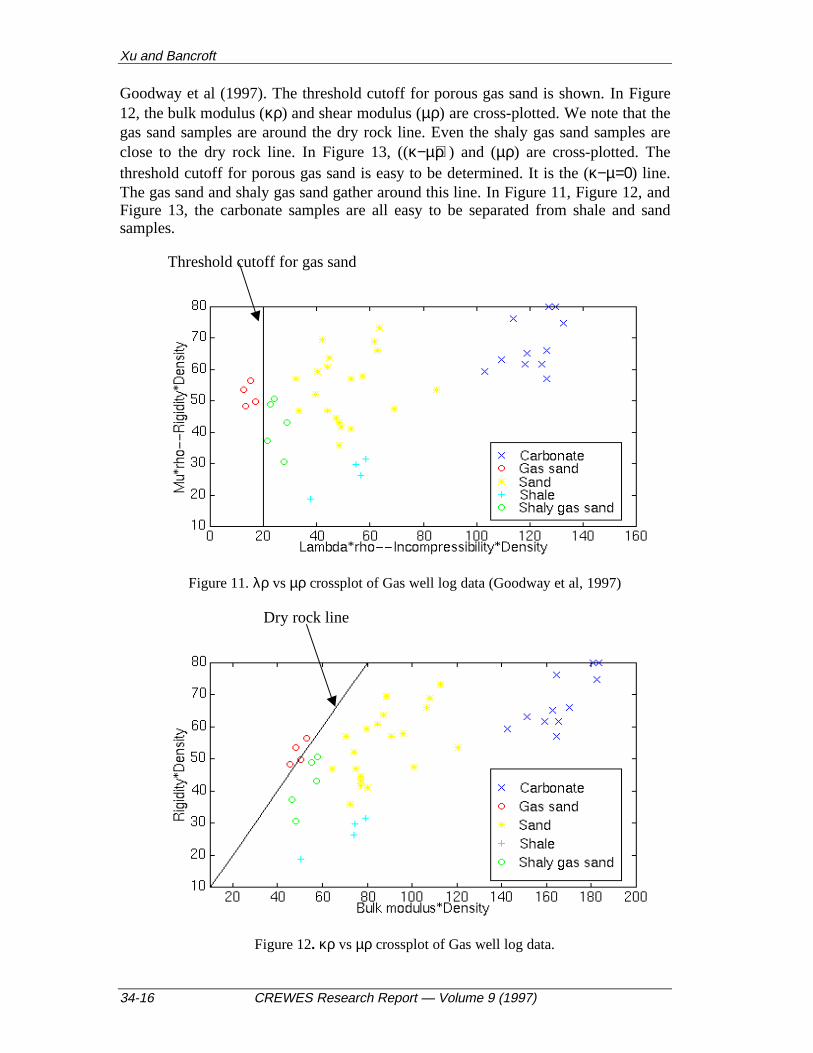
Goodway et al (1997). The threshold cutoff for porous gas sand is shown. In Figure12, the bulk modulus (κρ) and shear modulus (µρ) are cross-plotted. We note that thegas sand samples are around the dry rock line. Even the shaly gas sand samples areclose to the dry rock line. In Figure 13, ((κ−µ)ρ) and (µρ) are cross-plotted. Thethreshold cutoff for porous gas sand is easy to be determined. It is the (κ−µ=0) line.The gas sand and shaly gas sand gather around this line. In Figure 11, Figure 12, andFigure 13, the carbonate samples are all easy to be separated from shale and sandsamples.

Threshold cutoff for gas sand

Figure 11. λρ vs µρ crossplot of Gas well log data (Goodway et al, 1997)

Dry rock line

Figure 12. κρ vs µρ crossplot of Gas well log data.

AVO analysis

CREWES Research Report — Volume 9 (1997) 34-17

As gas causes κ in wet rock to change significantly, and µ does not change as gasfills the dry rock frame, we consider the sensitivity of (κ−µ) to detect the gas existingin rocks. The Table 2 gives various rock property values, from the young gas log dataused by Goodway et al (1997), and average % change i.e. contrast at the interface fordetectability As κ=λ+2/3µ, κ is not as sensitive to detect fluid as λ because thesensitivity is diluted by 2/3µ (i.e. non-pore fluid). However, the (κ−µ)=(λ−1/3µ) ismore sensitive than λ to detect the gas existing. And quantitatively, (κ−µ) is roundzero with gas in the rock. In Table 2 actual Vp, Vs, and ρ values from a shallow wellhave been combined to give various rock property values. Exceptκ, κ−µ, (κ−µ)/µ (bold), all other values are quoted from Goodway’s paper. Bycomparing the average percentage changes of λ and κ−µ, we note κ−µ is moresensitive than λ to variations in rock properties going from capping shale to gas sand.And the average % change of (κ−µ)/µ ratio is greater than the average % change ofλ/µ.

Threshold cutoff for gas sand

Figure 13. (κ−µ)ρ vs µρ crossplot of Gas well log data.

Vs Vp ρ

Shale 1290 2898 2.425

Gas Sand 1666 2857 2.275

∆Vs/Vs=0.25 ∆Vp/Vp=-0.014 ∆ρ/ρ= -0.064

Xu and Bancroft

34-18 CREWES Research Report — Volume 9 (1997)

Vp/Vs (Vp/Vs)2 σ λ+2µ λ µ κ λ/µ κ−µ (κ−µ)/µ

Shale 2.25 5.1 0.38 20.37 12.3 4.035 15.0 3.1 11.0 2.73

Gas sand 1.71 2.9 0.24 18.53 5.9 6.314 10.1 0.9 3.8 0.60

Avg. %change 27 55 45 9.2 70 44 39 110 97 128

Table 2. Shallow Gas Sand Log Measurements (Goodway et al, 1997)

Crossplots of elastic parameters in Blackfoot

Figure 14 shows cross-plots of the attributes of well 08-08 in Blackfoot survey. (a)shows p velocity, s velocity and density. (b) is the crossplot of p-velocity andvelocity. The linear regression is made and the line in (b) shows the fitting results.The Vp and Vs statistical relationship is Vp=1151+1.33Vs. (c) is the crossplot of p-velocity and density. The relationship between p-velocity and density is obtained byfitting: ρ=0.25Vp0.27. (d) is the crossplot of s-velocity and p-velocity showing thechannel sand in the circle. (e) is the crossplot of shear modulus (µ) and bulkmodulus.(κ). (f) is the crossplot of incompressibility (λ) and shear modulus (µ). (g) isthe crossplot of shear modulus (µ) and (λ+2µ). (h) is the crossplot of shear modulus(µ) and (κ−µ). The channel sand samples are in the circles. We note that in (e) thechannel sand samples are close to the dry line and in (f) and (h) the samples outsidethe channel are more scattered, and in (h), the (κ−µ) of channel sand samples areclose to threshold cutoff for gas existing.

(a) (b)

AVO analysis

CREWES Research Report — Volume 9 (1997) 34-19

(c) (d)

(e) (f)

(g) (h)

Figure 14. Cross-plots of well 08-08 in Blackfoot

(a) (b)

Xu and Bancroft

34-20 CREWES Research Report — Volume 9 (1997)

(c) (d)

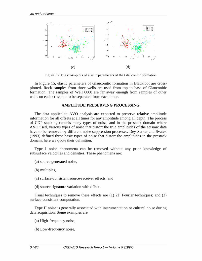
Figure 15. The cross-plots of elastic parameters of the Glauconitic formation

In Figure 15, elastic parameters of Glauconitic formation in Blackfoot are cross-plotted. Rock samples from three wells are used from top to base of Glauconiticformation. The samples of Well 0808 are far away enough from samples of otherwells on each crossplot to be separated from each other.

AMPLITUDE PRESERVING PROCESSING

The data applied to AVO analysis are expected to preserve relative amplitudeinformation for all offsets at all times for any amplitude among all depth. The processof CDP stacking cancels many types of noise, and in the prestack domain whereAVO used, various types of noise that distort the true amplitudes of the seismic datahave to be removed by different noise suppression processes. Dey-Sarkar and Svatek(1993) defined three basic types of noise that distort the amplitudes in the prestackdomain; here we quote their definition.

Type I noise phenomena can be removed without any prior knowledge ofsubsurface velocities and densities. These phenomena are:

(a) source generated noise,

(b) multiples,

(c) surface-consistent source-receiver effects, and

(d) source signature variation with offset.

Usual techniques to remove these effects are (1) 2D Fourier techniques; and (2)surface-consistent computation.

Type II noise is generally associated with instrumentation or cultural noise duringdata acquisition. Some examples are

(a) High-frequency noise,

(b) Low-frequency noise,

AVO analysis

CREWES Research Report — Volume 9 (1997) 34-21

(c) Drilling noise, and

(d) Channel imbalance problems.

Type III noises are entirely due to wave propagation effects in a visco-elasticmedium. They are

(a) 2D spherical divergence,

(b) thin bed attenuation,

(c) array attenuation,

(d) inelastic attenuation,

(e) curvature effects, and

(f) overburden transmission effects.

In general, wave propagation phenomena have a tendency to reduce the amplitudein the far offsets relative to near offsets. The trouble with this type of deterministiccorrection is two-fold:

(1) The knowledge of subsurface parameters necessary to compute the amplitudecorrections is often inadequate and sometimes nonexistent.

(2) The 2D inhomogeneity causes rapid variation of these parameters, thus makingthe deterministic corrections unreliable outside the point of control.

An approach advocated by Dey-Sarkar and Svatek (1993) is to calibrate theamplitudes using some statistical procedure. After the Type I and Type II noises areremoved from the prestack data, there are two components of the amplitude. The firstcomponent is associated with the amplitude variation due to Type III noise. Thesecond component is associated with the reflection coefficient variation with offset.We would like to extract the second component and remove the first component. Thiscannot be achieved by analyzing an event of interest, which is contaminated by thereflection coefficient variation. We estimate the first component (Type III noise)from a window of events above the target event. The rms amplitudes are computedfor each offset and an exponential decay function is fitted through the data points.The coefficient of this decay function is the amplitude correction factor for the event.The coefficient is spatially averaged to obtain a smoothly varying function. Theadvantages of this technique are, (1) the robustness, (2) no subsurface parameters areassumed, and (3) no distortion is produced in the data because of the slowly varyingfunction. In this paper, we choose difference time window and CDP location tocalculate the correction factors and interpolate these sparse factors to obtaincorrection factor for each time and CDP location. The final correction factors aretime and laterally various. Figure 17 is an example using above technique. Panel (b)is the amplitude preserved processing result from panel (a). Panel (c) is the syntheticgather from the well log nearby. The left most trace in each panel is the stack trace

Xu and Bancroft

34-22 CREWES Research Report — Volume 9 (1997)

from panel (a). Compared with gather on Panel (a), the gather on Panel (b) isimproved.

(a) (b) (c)

Figure 17. (a) the gather before amplitude calibration. (b) the gather after amplitudecalibration. (c) the synthetic gather.

EXTRACTIONS OF ELASTIC PARAMETERS FROM

BLACKFOOT 10 HZ VERTICAL DATA

Least square regression analysis and inversion are the common approaches in theAVO analysis. Parson (1986) obtained contrasts of three elastic parameters (λ, µ, andρ) by pre-stack inversion. Goodway et al (1997) obtained the Vp and Vs frominversion and converted them to the λ/µ to detect the reservoirs. However, thenonuniqueness is always the problem in the seismic inversion. The backgroundvelocity error causes the ratio change greatly or eliminates the high frequencycontrast. Appropriate selection of parameters, background velocity, waveletestimation, application of a priori information are still important issues which remainto be resolved. Here we choose the least square regression analysis to extract elasticparameters from pre-stack data. The extraction provides band-limited information.And we also invert the band-limited result by recursive inversion and model-basedinversion. In the regression analysis, we express the P-P and P-S reflectioncoefficient equations with the elastic parameters (λ and µ, or κ and µ) and extractthese parameters directly without conversion from velocity.

Expressing reflection coefficients with elastic parameters

Some authors pointed out the need for a more physical insight afforded by elasticparameters (Castagna et al. 1993, Stewart 1995, Goodway et al 1997) in theapproximation of reflection coefficients. Castagna (1993) also indicated the bulkmodulus that is embedded in Vp links velocity with rock properties for pore fluiddetection. So we may benefit from the conversion from velocity measurements tomodulus parameters of rigidity (µ), bulk modulus (κ), incompressibility (λ).

Aki-Richards’ reflection coefficient formula for P-P reflection can be rewritten asthe combination of contrasts of incompressibility (λ), shear modulus (µ), and density(ρ) (Parson 1986, Goodway et al. 1997) as follows:

AVO analysis

CREWES Research Report — Volume 9 (1997) 34-23

ρρ∆−+

µµ∆−

µ+λµ+λ∆+= )2tan1(

4

12sin2)(2)2(

)2()2tan1(

4

1ii

Vp

VsiPP (21)

Goodway et al. (1997) thought this equation not practical for AVO analysis andmodified it as the impedance contrasts as equation (22). The third term in equation(22) can be cancelled with the approximations of Vp/Vs>2 and tani~sini. Afterinverting the seismic data to Vp and Vs information and using the moduli toimpedance relationships to obtain the λρ and µρ, the ratio of λ/µ may be obtained.The advantages of this scheme used by Goodway et al (1997) are less unknowns andmore robustness in the AVO analysis, but the low frequency information ofimpedance is usually not accurate from inversions which influences ratio of λ/µ thedetectability of anomalies.

ρρ∆−−∆−∆+= ]2sin2)(22tan

2

1[2sin2)(8)2tan1( i

Vp

Vsi

Is

Isi

Vp

Vs

Ip

IpiPP (22)

(a) (b) (c)

(d) (e) (f)

Xu and Bancroft

34-24 CREWES Research Report — Volume 9 (1997)

(g) (h) (i)

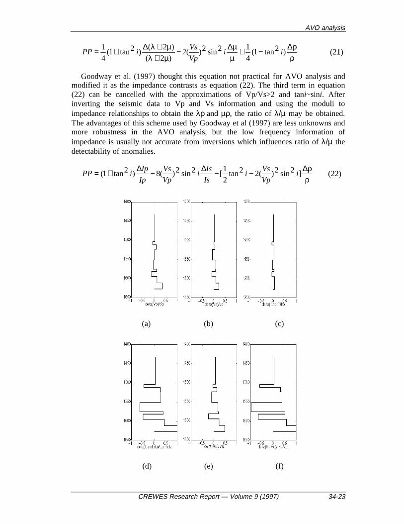
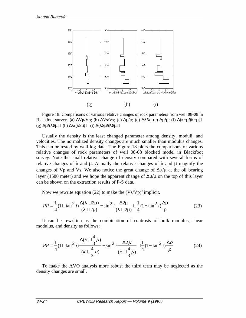
Figure 18. Comparisons of various relative changes of rock parameters from well 08-08 inBlackfoot survey. (a) ∆Vp/Vp; (b) ∆Vs/Vs; (c) ∆ρ/ρ; (d) ∆λ/λ; (e) ∆µ/µ; (f) ∆(κ−µ)/(κ−µ);(g) ∆µ/(λ+2µ);(h) ∆λ/(λ+2µ); (i) ∆(λ+2µ)/(λ+2µ).

Usually the density is the least changed parameter among density, moduli, andvelocities. The normalized density changes are much smaller than modulus changes.This can be tested by well log data. The Figure 18 plots the comparisons of variousrelative changes of rock parameters of well 08-08 blocked model in Blackfootsurvey. Note the small relative change of density compared with several forms ofrelative changes of λ and µ. Actually the relative changes of λ and µ magnify thechanges of Vp and Vs. We also notice the great change of ∆µ/µ at the oil bearinglayer (1580 meter) and we hope the apparent change of ∆µ/µ on the top of this layercan be shown on the extraction results of P-S data.

Now we rewrite equation (22) to make the (Vs/Vp)2 implicit.

ρρ∆−+

µ+λµ∆−

µ+λµ+λ∆+= )2tan1(

4

1

)2(

22sin)2(

)2()2tan1(

4

1iiiPP (23)

It can be rewritten as the combination of contrasts of bulk modulus, shearmodulus, and density as follows:

ρρ

µκ

µ

µκ

µκ ∆−++

∆−+

+∆+= )2tan1(

4

1

)3

4(

22sin)

3

4(

)3

4(

)2tan1(4

1iiiPP (24)

To make the AVO analysis more robust the third term may be neglected as thedensity changes are small.

AVO analysis

CREWES Research Report — Volume 9 (1997) 34-25

)2(

22sin)2(

)2()2tan1(

4

1

µ+λµ∆−

µ+λµ+λ∆+≈ iiPP (25)

Another way to make equation (24) two-term expression is to incorporate the thirdterm into the first term. Gardner’s relationship is fit to a very wide range of velocitiesand porosities. Gardner’s relationship between density and P wave velocity is

bPaV=ρ (b=0.25), (26)

And the relationship between moduli, density and P wave velocity is

ρµ+λ= 2

PV , (27)

From equation (26) and equation (27), an approximation of equation (24) isobtained as:

)2(

22sin)2(

)2()2tan

9

8

9

10(

4

1

µ+λµ∆−

µ+λµ+λ∆+≈ iiPP (28)

or

)2()2sin42tan

9

8

9

10(

2

1

)2()2tan

9

8

9

10(

4

1

µ+λµ∆−++

µ+λλ∆+≈ iiiPP (28)’

P-S reflection coefficient can also be simplified and associated with rockproperties. Aki-Richards approximation for P-S reflection coefficient can bereformulated in terms of rigidity and density as:

)]cos(2[tan2

1jijPS +

µµ∆

αβ+

ρρ∆

βα−= (29)

]sin)1()2[(tan2

1 22 jjPS +βα

µµ∆

αβ−

µµ∆

αβ+

ρρ∆

βα−= (30)

In fact the equation (29) reveals the AVO variation for shear modulus and ρ term.The slope of P-S wave AVO is primarily dependent on the shear modulus.

As 2

1~

αβ

,

)]cos([tan jijPS +µµ∆+

ρρ∆−≈ (31)

Xu and Bancroft

34-26 CREWES Research Report — Volume 9 (1997)

]sin2

94[tan 2 jRjPS SS µ

µ∆−−−≈ (32)

where )(2

1

ββ∆+

ρρ∆−=ssR is the reflectivity of the normal incidence of the SH

wave.

AVO analysis of P-S data

In theory, equation (31) and equation (32) can be applied to AVO analysis to getthe density and rigidity relative differences if the incident angles and reflection anglesare known. However, the incident P wave path and converted S wave path even in thehorizontal homogeneous media are not symmetrical like the incident P wave path andreflected P wave path. It is not easy to obtain the incident angles or reflection anglesfor the P-S reflection and the Vp/Vs ratio is necessary even for the single interfacecase. In addition, the seismic data are usually sorted in common mid-point (CMP)gather form, and the conversion from CMP gather to common converted point (CCP)gather is the usual process in the P-S seismic data processing.

Figure 19. Illustration of propagation of incidence and converted wave.

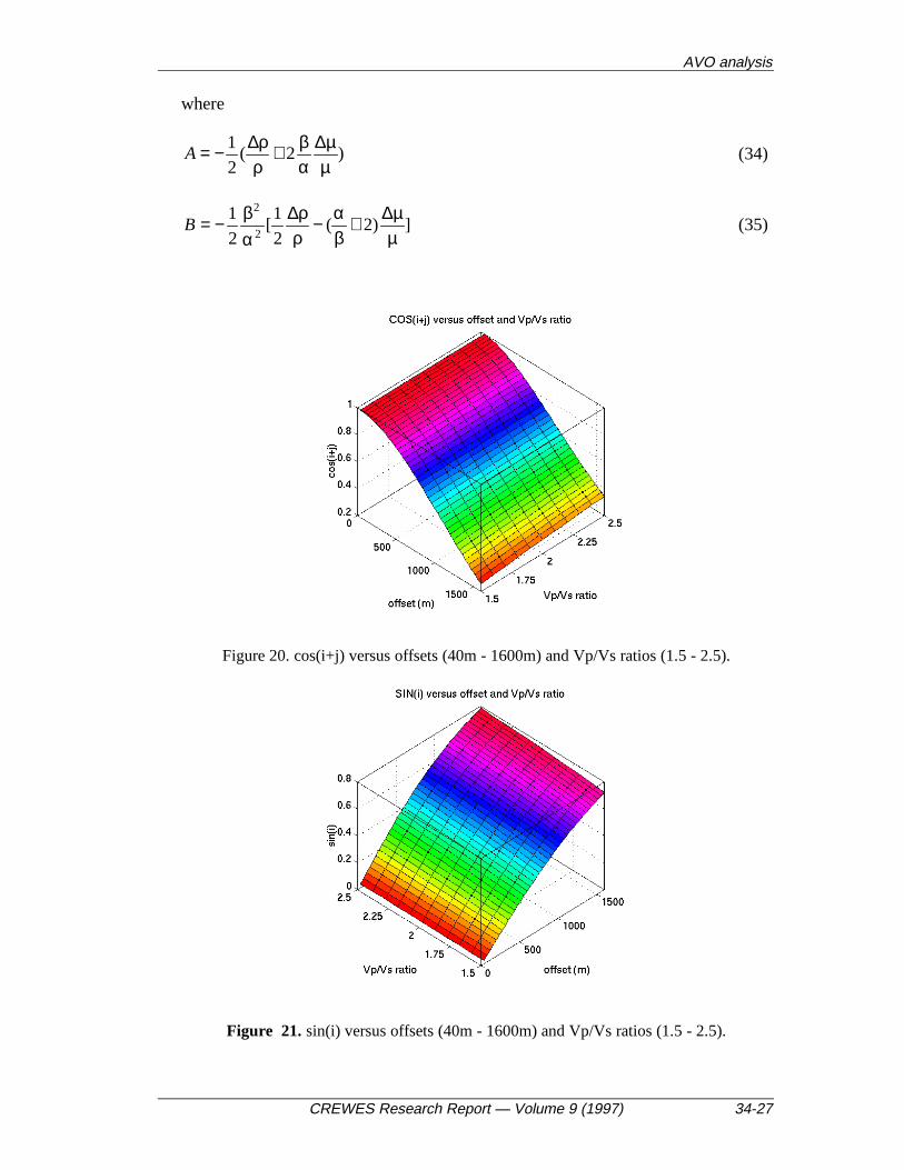
Figure 19 illustrates the moving of converted point as the Vp/Vs ratio changesgiven fixed source and receiver positions. In the extraction of AVO, Vp/Vs ratio isusually approximated to a constant such as 2.0 . Now we check the influence ofvarying Vp/Vs ratio on the incident and converted angles. In Figure 20 the cos(i+j) inequation (31) is plotted with variation versus offsets and Vp/Vs ratios. And in Figure21 the sin(i) is plotted with variation versus offsets and Vp/Vs ratios. And also inFigure 22 the sin(j) is plotted with variation versus offsets and Vp/Vs ratios. Twopoints are observed on these three figures.

sin(i) slowly varies as Vp/Vs ratio varies; and sin(j) varies as Vp/Vs ratio varies;These two kinds of changes cancel each other to make the cos(i+j) change slowlywith variation of Vp/Vs ratio.

There should be smaller error to use the cos(i+j) than sin2j under the assumption ofconstant Vp/Vs. Therefore it is better to use sin(i) or cos(i+j) to AVO analysis insteadof sin(j). The equation (32) can be expressed as the function of sin(i) as follow.

iBiAPS 3sinsin +≈ (33)

AVO analysis

CREWES Research Report — Volume 9 (1997) 34-27

where

)2(2

1

µµ∆

αβ+

ρρ∆−=A (34)

])2(2

1[

2

12

2

µµ∆+

βα−

ρρ∆

αβ−=B (35)

Figure 20. cos(i+j) versus offsets (40m - 1600m) and Vp/Vs ratios (1.5 - 2.5).

Figure 21. sin(i) versus offsets (40m - 1600m) and Vp/Vs ratios (1.5 - 2.5).

Xu and Bancroft

34-28 CREWES Research Report — Volume 9 (1997)

Figure 22. sin(j) versus offsets (40m - 1600m) and Vp/Vs ratios (1.5 - 2.5).

The AVO weighted stack was first mentioned by Smith and Gidlow (1987) It is infact the least squared linear regression analysis. Ferguson (1996) inverted theBlackfoot 3C data by the weighted stack technique. The P velocity and S velocitywere obtained by band-limited inversion and the Vp/Vs ratio was obtained from theinverted P and S velocity information. Here we hope to apply another scheme toextract the elastic parameter from the P-S data. From equation (31), the least squareregression can be employed to extract the contrasts of density and shear modulus. Wehope to get the relative reliable density contrast from the extraction. And also thecontrast of shear modulus can test the extraction result from P-P data. Because of themore difficulties to process radial component data set to obtain the preservedamplitude, good aligned events, and corrected incident and reflected angles, effortsare still making on the Blackfoot data sets and reasonable results will be shown innear future.

Elastic parameter extraction from Blackfoot 10 Hz vertical

Pre-stack seismic data were acquired from 10 Hz Blackfoot seismic data set, withpreliminary processing and amplitude-preserving processing applied.

(a) (b)

AVO analysis

CREWES Research Report — Volume 9 (1997) 34-29

(c)

Figure 23 Well 0808 and synthetic gather from the well

Figure 23 are the well logs of well 0808 and the synthetic gather (Margrave et al,1995, Potter et al, 1996). The Glauconitic channel formation is shown on the welllogs. From the P-wave velocity and density contrasts, the channel sand is Class IIIsand (Rutherford and Williams, 1989) with low P impedance in sand. However theimpedance changes is not much, and on the synthetic gather the AVO anomaly is notsignificant.

Using equation (28), the relative contrasts, µ+λµ+λ∆

2

)2( and

µ+λµ∆2

are obtained by

linear regression. By combining these contrasts, the contrasts of µ+λ

λ∆2

,µ+λµ−κ∆

2

)(

and γγ∆

are also derived,

where βα=γ / is the Vp/Vs ratio and

)2

2

2(

2

1)

2

)2(

2(

2

1 2

µ+λµ∆−

µ+λλ∆≈

µ+λµ∆−γ−

µ+λλ∆=

γγ∆

Figure 24 shows the above five contrasts within the seismic frequency bandwidth(5-10-60-70 Hz).

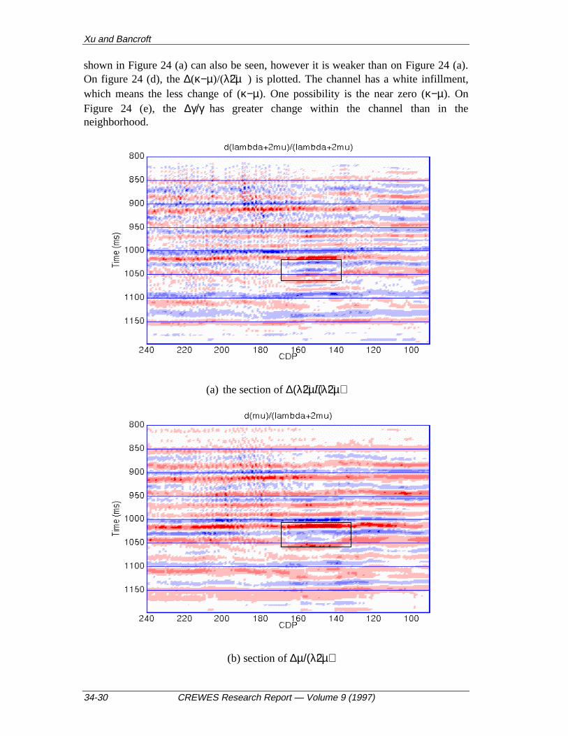
In Figure 24 (a) the contrast of ∆(λ+2µ)/(λ+2µ) shows anomaly in the box (cdp130-170, time 1000ms-1100ms) which is the approximated location of Glauconiticchannel. The box shows the zone with difference from neighborhood. The extracted∆µ/(λ+2µ) section is displayed in Figure 24 (b). In the box on Figure 24 (b), theGlauconitic channel shape can be been. But on the top and bottom and in between the∆µ/(λ+2µ) changes continuously from the neighbor zones. Figure 24 (c) is obtainedby subtraction of two times (b) from (a). It approximates ∆λ/(λ+2µ).The anomaly

Xu and Bancroft

34-30 CREWES Research Report — Volume 9 (1997)

shown in Figure 24 (a) can also be seen, however it is weaker than on Figure 24 (a).On figure 24 (d), the ∆(κ−µ)/(λ+2µ) is plotted. The channel has a white infillment,which means the less change of (κ−µ). One possibility is the near zero (κ−µ). OnFigure 24 (e), the ∆γ/γ has greater change within the channel than in theneighborhood.

(a) the section of ∆(λ+2µ)/(λ+2µ)

(b) section of ∆µ/(λ+2µ)

AVO analysis

CREWES Research Report — Volume 9 (1997) 34-31

(c) the section of ∆λ/(λ+2µ)

(d) the section of ∆(κ−µ)/(λ+2µ)

Xu and Bancroft

34-32 CREWES Research Report — Volume 9 (1997)

(e) the section of ∆γ/γ (γ is the Vp/Vs ratio).

Figure 24. the analysis results of Blackfoot vertical seismic data.

Figure 25 shows the inversion results from the extraction sections in figure 24.The low frequency components are obtained from the wells. The recursive integrationof the AVO extraction sections in Figure 24 is merged with the low frequencycomponents.

(a) λ

AVO analysis

CREWES Research Report — Volume 9 (1997) 34-33

(b) λ+2µ

(c) µ

Figure 25. The inversion results from Figure 24.

ZERO OFFSET STACK

It is well recognized that amplitude and phase variation versus offset may causeCDP stacking to degrade reflection data quality. The extraction of the intercepts byleast squares regression produces a “zero offset” stack (Denhem et al, 1985, coruhand Demirbag, 1989). On the other hand, we hope to obtain reservoir information byvarious approaches to overcome the limits of seismic data. The zero offset sectionprovides (1) a better approximation to the normal incidence P-wave reflectioncoefficient, (2) broader bandwidth and higher frequencies, and (3) high resolution.Seismic impedance traces inverted from zero offset stack traces should be superior tofrom conventional seismic stack sections.

Approximation of P-P reflectivity in term of offsets

Xu and Bancroft

34-34 CREWES Research Report — Volume 9 (1997)

Aki-Richards approximation of P-P reflectivity can be written as

iCiBAPP 42 tantan ++= (36)

where

)(2

1

αα∆+

ρρ∆=A

ββ∆−

ρρ∆−

αα∆= 42

2

1B

)(2ββ∆+

ρρ∆−=C

Figure 26 Reflection of compressional wave at the interface of media.

If the wave propagation path is shown as Figure 26, the P-P reflectivity canexpressed as function of offsets as

42 ’’ xCxBAPP ++= (37)

where

)(2

1

αα∆+

ρρ∆=A

)4/()422

1(’ 2zB

ββ∆−

ρρ∆−

αα∆=

)8/()(2’ 4zCββ∆+

ρρ∆−=

Therefore, the AVO analysis can be done by curve fitting of the offsets. And the Ain the above equation is independent on the changes of variables of x or sini. And thenormal incidence reflectivity is easy to be obtained in the AVO analysis.

AVO analysis

CREWES Research Report — Volume 9 (1997) 34-35

Even with an incident angle of 45 degrees recovery of the third term is less robustthan second term recovery. Therefore another further approximation is commonlyused.

2’xBAPP += (37)’

AVO in F-X domain

Consider the convolutional earth model. The seismic trace is expressed as theconvolution of reflectivity and wavelet as (38)

T(t,x) = R(t,x) * W(t) (38)

Where T(t) is the seismic trace, R(t) is the reflectivity, and W(t) is the wavelet.

R(t,x) = A(t) + B(t) x2 + C(t) x4

T(t,x) = A(t)*W(t) + B(t)*W(t) x2 + C(t)*W(t) x4

T(t,x) = P(t) + Q(t) x2 + S(t) x4

T(f,x) = P(f) + Q(f) x2 + S(f) x4 (39)

T(f,x) = P(f) + Q(f) x2 (39’)

where T = P, Q ,and S are the spectra of P, Q, and S.

Figure 27 Comparison of normal incidence trace, stack trace, and fitting traces in timedomain and frequency domain.

In Figure 27, the first 16 traces in the left are of the same CDP gather. Trace 19labeled as ‘A’ is normal incidence trace coming from convolution of zero offsetreflectivity and wavelet. Trace 22 labeled as ‘B’ is the stack trace, and trace 23(labeled as ‘C’) is the error of stack trace. Trace 26 with label ‘D’ is the fitting tracein time domain and trace 27 with label ‘E’ is the error of trace 26. Trace 30 labeled as

Xu and Bancroft

34-36 CREWES Research Report — Volume 9 (1997)

‘F’ is the fitting trace in frequency domain and trace 31 labeled as ‘G’ is the error oftrace 30. Here the fitting traces are using the second order approximation. The fittingtraces are closer to the normal incidence trace both for the t-x domain and f-xdomain.

Figure 28. Comparison of errors of traces from different methods.

In Figure 28, the errors of traces from different methods are compared. Trace 1 isthe error of stack trace. Trace 2 is the error of fitting trace in t-x domain by equation(37’). Trace 3 is the error of fitting trace in f-x domain by equation (39’). Trace 4 andtrace 5 are the errors of fitting traces in t-x domain and f-x domain with by equation(37) and equation (39). From the comparison, three points are concluded: first, thefitting trace has smaller error than stack trace; second, the higher order approximationfitting trace has smaller error than the low higher order approximation fitting trace;and last, the results in the t-x domain and f-x domain are equivalent.

Figure 29 displays real parts (left panel) and imaginary parts (right panel) of thespectra of each trace in the CDP gather used to curve fitting. The spectrum value forfrequency greater than 125 Hz is zero in this case. Therefore, the curve fitting for thebig frequency band is not necessary, and the calculation is saved. That compensatesthe cost of fast Fourier transform. The following values compare the running times oft-x and f-x domain curving fitting.

The CDP gather has 12 traces, 128 samples, and time sample rate 0.1s. Therunning time in t-x domain is 0.331s and in f-x domain 0.229s.

AVO analysis

CREWES Research Report — Volume 9 (1997) 34-37

Figure 29. The real parts (left) and the imaginary parts (right) of spectra of the CDP gather.

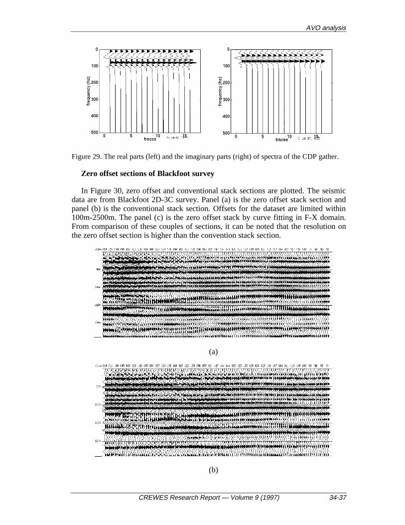
Zero offset sections of Blackfoot survey

In Figure 30, zero offset and conventional stack sections are plotted. The seismicdata are from Blackfoot 2D-3C survey. Panel (a) is the zero offset stack section andpanel (b) is the conventional stack section. Offsets for the dataset are limited within100m-2500m. The panel (c) is the zero offset stack by curve fitting in F-X domain.From comparison of these couples of sections, it can be noted that the resolution onthe zero offset section is higher than the convention stack section.

(a)

(b)

Xu and Bancroft

34-38 CREWES Research Report — Volume 9 (1997)

(c)

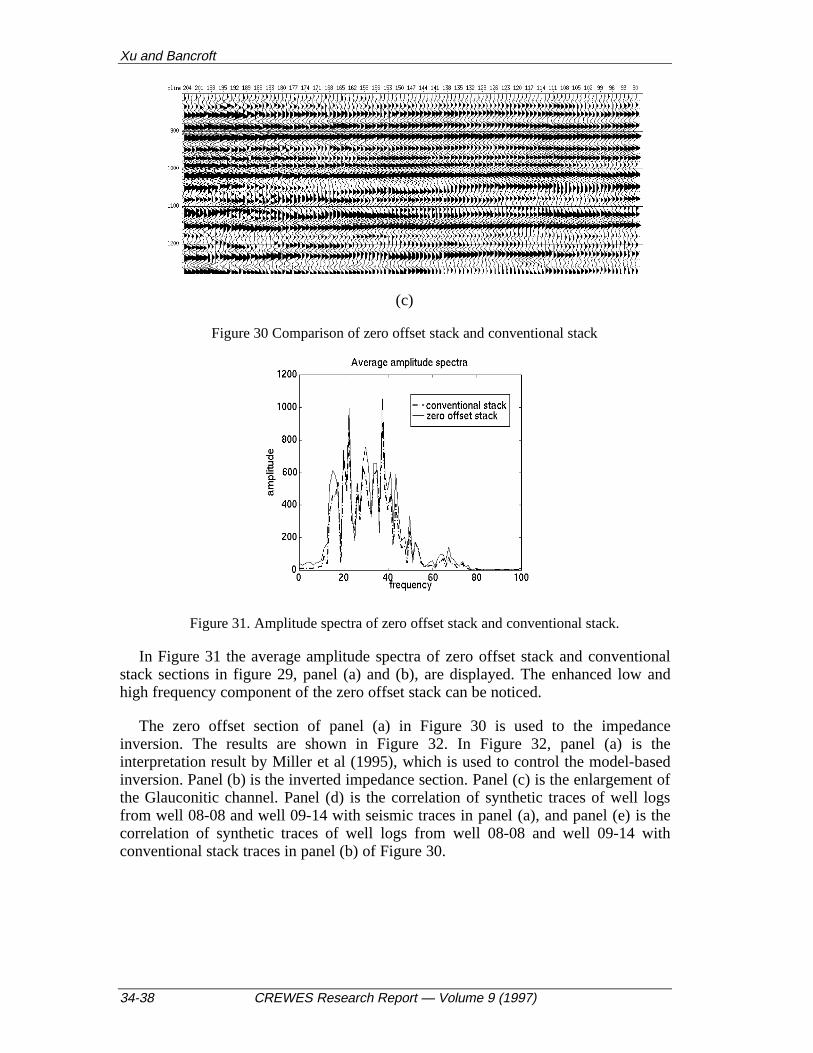
Figure 30 Comparison of zero offset stack and conventional stack

Figure 31. Amplitude spectra of zero offset stack and conventional stack.

In Figure 31 the average amplitude spectra of zero offset stack and conventionalstack sections in figure 29, panel (a) and (b), are displayed. The enhanced low andhigh frequency component of the zero offset stack can be noticed.

The zero offset section of panel (a) in Figure 30 is used to the impedanceinversion. The results are shown in Figure 32. In Figure 32, panel (a) is theinterpretation result by Miller et al (1995), which is used to control the model-basedinversion. Panel (b) is the inverted impedance section. Panel (c) is the enlargement ofthe Glauconitic channel. Panel (d) is the correlation of synthetic traces of well logsfrom well 08-08 and well 09-14 with seismic traces in panel (a), and panel (e) is thecorrelation of synthetic traces of well logs from well 08-08 and well 09-14 withconventional stack traces in panel (b) of Figure 30.

AVO analysis

CREWES Research Report — Volume 9 (1997) 34-39

(a)

(b)

(c)

(d)

Xu and Bancroft

34-40 CREWES Research Report — Volume 9 (1997)

(e)

Figure 32. the inversion of zero offset stack section.

The inversion in Figure 32 is done by Hampson-Russell Strata. Although on panel(c) and panel (d) of Figure 32 the channel sand can be traced clearly, we must keep inmind the inversion results depend on wide band model building. However thecorrelation between seismic traces and synthetic traces on the zero offset stack aremuch superior to on the conversion stack.

CONCLUSIONS

Aki-Richards’ approximation of P-S reflection coefficient has greater error thanAki-Richards’ approximation of P-P reflection coefficient in the great propertycontrast cases, especially when S wave property changes a lot.

Aki-Richards’ approximation of P-S coefficient is good for intermediate incidentangle range and less changing S wave property.

The bulk modulus and shear modulus of dry rock are approximately equal and thegas bearing rock behaves as dry rock. The water saturation cause the bulk modulusincreases rapidly. This determines the difference between the bulk modulus and shearmodulus is very sensitive to the gas existing in the rocks.

P-S AVO extraction has more difficulties to be done than the P-P extractionbecause of the gather binning, statics, and noise levels.

Zero offset stack section has better resolution than conventional stack section. Andthe inversion of zero offset section shows good correlation between well logs andseismic traces in the Blackfoot.

P-P and P-S reflection coefficients can be expressed as the contrasts of elasticparameters and be applied in the linear regression analysis. The extraction of elasticparameter from Blackfoot 10 Hz vertical shows the reasonable results.

AVO analysis

CREWES Research Report — Volume 9 (1997) 34-41

FUTURE WORK

Because of the relative lower S/N ratio of radial data, the analysis is tougher. Thestatics on the radial component are greater than on the vertical component. Thecareful processing is necessary. Now the authors are making efforts to process theBlackfoot data to obtain the high quality data to be used to AVO extraction.

In the meantime, the AVO inversion is considering to be employed as anotherapproach. We would like the elastic earth model reconstruction by inversion. Theconverted wave information may help to constrain the inversion.

ACKNOWLEDGMENTS

We would like to thank sponsors of CREWES Project.

Thank Henry Bland and Darren Foltinek for their technical assistant in completingthe project.

REFERENCES

Aki, K. I. and Richards, P. G., 1980, Quantitative seismology: W.H. Freeman and CO.Behle, A. and Dohr, G. 1985, Converted waves in exploration seismic in Seismic Shear Waves, G.

Dohr (ed.), 178-220. Handbook of Geophysical Exploration, Vol. 15b. Geophysical Press.Bortfeld, R., 1961, Approximation to the reflection and transmission coefficients of plane

longitudinal and transverse waves: Geophys. Prosp., 9, 485 - 502.Castagna, J. P., Batzle, M. L. and Eastwood, R. L., 1985, Relationship between compressional wave

and shear wave velocities in clastic silicate rocks: Geophysics, V. 50, 571 - 581.Castagna, J. P., 1993, Petrophysical imaging using AVO: The Leading Edge, March, 1993, 172-178.Castagna, J. P., Batzle, M. L. and Kan, T. K., 1993, Rock physics: the link between rock properties

and AVO response in Castagna, J. P., and Backus, M. M., Eds., Offset-dependentreflectivity--Theory and practice of AVO analysis, Soc. Expl. Geophys., 135-171.

Chiburis, E., F., 1993, AVO applications in Saudi Arabia in Castagna, J. P., and Backus, M. M.,Eds., Offset-dependent reflectivity--Theory and practice of AVO analysis, Soc. Expl.Geophys., 211-229.

Chung, W. Y., and Corrigan, D., 1985, Gathering mode-converted shear waves: a model study: 55thSEG meeting, Washington, Expanded Abstracts, 602-604.

Dahl, T., and Ursin, B., 1991, Parameter estimation in a one-dimensional anelastic medium, Journalof Geophysical Research, V 96, 20,217 - 20, 233.

Dey-Sarkar, S. K., and Svatek, S. V., Prestack analysis – An integrated approach for seismicinterpretation in Clastic basins in Castagna, J. P., and Backus, M. M., Eds., Offset-dependent reflectivity--Theory and practice of AVO analysis, Soc. Expl. Geophys., 57-77.

Ferguson, R. J., P-P and P-S inversion of 3-C seismic data: Blackfoot, Alberta: CREWES ResearchReport 1995, Chapter 41.

Goodway, B., Chen, T., and Downton, J., 1997, Improved AVO fluid detection and lithologydiscrimination using Lame petrophysical parameters; “λρ”, “ µρ”, and “λ/µ fluid stack”,from P and S inversions: CSEG national convention, Expanded Abstracts, 148-151.

Goodway, B., Chen, T., and Downton, J., 1997, Improved AVO fluid detection and lithologydiscrimination using Lame petrophysical parameters; “λρ”, “ µρ”, and “λ/µ fluid stack”,from P and S inversions: 67th Ann. Internat. Mtg., Soc. Expl. Geophys., ExpandedAbstracts.

Garotta, R., 1988, Amplitude-versus-offset measurements involving converted waves: 58th Ann.Internat. Mtg., Soc. Expl. Geophys., Expanded Abstracts, 1357.

Xu and Bancroft

34-42 CREWES Research Report — Volume 9 (1997)

Hampson, D., and Russell, B., 1990, AVO inversion: theory and practice: 60th Ann. Internat. Mtg.,Soc. Expl. Geophys., Expanded Abstracts, 1456-1458.

Koefoed, O., 1955, On the effect of Poisson’s ratio of rock strata on the reflection coefficients ofplane waves: Geophs. Prosp., 3, 381-387.

Lindseth, R. O., 1979, Synthetic sonic logs -- a processing for stratigraphic interpretation:Geophysics, V. 44, No 1, 3 -26.

Margrave, G. F., Foltinek, D. S., 1995, P-P and P-SV cross sections: CREWES Research Report1995, Chapter 5.

Miller, S. L. M., Aydemir, E. O., and Margrave, G. F., 1995, Preliminary interpretation of P-P and P-S seismic data from the Blackfoot broad-band survey: CREWES Research Report 1995,Chapter 42.

Parson, R., 1986, Estimating reservoir mechanical properties using constant offset images ofreflection coefficients and incident angles: 56th Ann. Internat. Mtg., Expanded Abstracts,617-620.

Pigott, J. D., Shrestha, R. K., and Warwick, R. A., 1990, Direct determination of Carbonate reservoirporosity and pressure from AVO inversion: 60th Ann. Internat. Mtg., Soc. Expl. Geophys.,Expanded Abstracts, 1533-1536.

Potter, C. C., Miller, S. L. M., and Margrave, G. F., 1995, Formation elastic parameters andsynthetic P-P and P-S seismograms for the Blackfoot field: CREWES Research Report1995, Chapter 37.

Rutherford, S. R. and Williams, R. H., 1989, Amplitude-versus-offset variation in gas sands:Geophysics, 54, 680-688.

Simin, V., Margrave, G. F., and Yang G. Y. C., AVO measurements for P-P and P-S data inBlackfoot 3C-3D dataset: CREWES Research Report 1995, Chapter 42.

Smith, G. C., and Gidlow, P. M., 1987, Weighted stacking from rock property estimation anddetection of gas: Geophys. Prosp. 35, 993-1014.

Spratt, R. S., Goins, N. R., and Fitch, T. J., 1993, Pseudo-shear: The analysis of AVO in Castagna, J.P., and Backus, M. M., Eds., Offset-dependent reflectivity--Theory and practice of AVOanalysis, Soc. Expl. Geophys., 37-56.

Shuey, R. T. 1985, A simplification of the Zoeppritz equations: Geophysics, V 50, 609 - 614.Stewart, R. R., Zhang, Q., and Guthoff, F., 1995, Relationships among elastic-wave values (Rpp, Rps,

Rss, Vp, Vs, ρ, σ, κ): CREWES Research Report 1995, Chapter 10.Swan, H. W., 1991, Amplitude-versus-offset measurement errors in a finely layered medium:

Geophysics, 56, 41-49.Taylor, G., The point of P-S mode-converted reflection: An exact determination: Geophysics, 54,

1060-1063.Tessmer, G., and Behle, A., 1988, Common reflection point data-stacking technique for converted

waves: Geophys. Prosp., V 36, 671-688.Verm, R. W., and Hilterman, F. J., 1994, Lithologic color-coded sections by AVO cross plots: The

Leading Edge, August, 847 - 853.Yu, G., 1985, Offset-amplitude variation and controlled-amplitude processing: Geophysics, 50,

2697-2708.Zheng, X., 1992, United formulas for reflection and transmission in potential: Presented at the 62nd

Annual International SEG Meeting, New Orleans, abstr. book, 1282-1284.Zhong, B., Zhou, X., Liu, X., and Jiang, Y., A new strategy for CCP stacking: Geophysics, 60, 517-

521.

AVO analysis

CREWES Research Report — Volume 9 (1997) 34-43

APPENDIX

Zoeppritz equations of P-P and P-S reflection coefficients

Aki and Richards (1980) give the Knot-Zoeppritz equations in convenient forms.For completeness the reflection coefficients of the incident P wave and reflected Pwave and S wave are shown as follows:

D/])coscos

()coscos

[( 2

1

1

1

1

2

2

1

1 Hpji

daFi

ci

bPPβα

+−α

−α

=

)D/()coscos

(cos

2 112

2

2

2

1

1 βαβα

+α

−= pji

cdabi

PS

where

βρ−β−αρβρβ−αρ−β−βρβρβ−βρβρ

β−β−α−α

2222

222221

211

22111

222222

222

221111

211

2211

2211

cos2)21(cos2)21(

)21(cos2)21(cos2

coscos

coscos-

=M

jppjpp

pippip

pipi

jpjp

)21()21( 2211

2222 ppa β−ρ−β−ρ= , 22

1122

22 2)21( ppb βρ+β−ρ= ,

2222

2211 2)21( ppc βρ+β−ρ= , )(2 2

11222 βρ−βρ=d ,

2

2

1

1 coscos

α+

α= i

ci

bE , 2

2

1

1 coscos

β+

β= j

cj

bF ,

2

2

1

1 coscos

βα−= ji

daG , 1

1

2

2 coscos

βα−= ji

daH ,

and

)/()M(detD 21212 ββαα=+= GHpEF .

The angles of i1, i2, j1, andj2 are shown on Figure A-1.

Xu and Bancroft

34-44 CREWES Research Report — Volume 9 (1997)

In c id e n t P

r e f le c t e d P

r e f le c t e d S

t r a n s m it t e d Pt r a n s m it t e d S

i 1

i 2

j 1

j 2

i 1

ρ1 α 1 β1

ρ2 α 2 β2

Figure A-1. Waves generated at an interface by an incident P-wave