JOHN N. FLEMING - University of New Brunswick · design of a semi-automatic algorithm for shoreline...
163
DESIGN OF A SEMI-AUTOMATIC ALGORITHM FOR SHORELINE EXTRACTION USING SYNTHETIC APERTURE RADAR (SAR) IMAGES JOHN N. FLEMING June 2005 TECHNICAL REPORT NO. 231
Transcript of JOHN N. FLEMING - University of New Brunswick · design of a semi-automatic algorithm for shoreline...

DESIGN OF A SEMI-AUTOMATIC ALGORITHM FOR
SHORELINE EXTRACTION USING SYNTHETIC
APERTURE RADAR (SAR) IMAGES
JOHN N. FLEMING
June 2005
TECHNICAL REPORT NO. 217
TECHNICAL REPORT NO. 231

DESIGN OF A SEMI-AUTOMATIC ALGORITHM FOR SHORELINE
EXTRACTION USING SYNTHETIC APERTURE RADAR (SAR) IMAGES
John N. Fleming
Department of Geodesy and Geomatics Engineering University of New Brunswick
P.O. Box 4400 Fredericton, N.B.
Canada E3B 5A3
June 2005
© John Fleming 2004

PREFACE
This technical report is an unedited reproduction of a thesis submitted in partial
fulfillment of the requirements for the degree of Master of Science in Engineering in the
Department of Geodesy and Geomatics Engineering, September 2004. The research was
supervised by Dr. Yun Zhang and Dr. David E. Wells.
As with any copyrighted material, permission to reprint or quote extensively from this
report must be received from the author. The citation to this work should appear as
follows:
Fleming, John N. (2005). Design of a Semi-Automatic Algorithm for Shoreline
Extraction using Synthetic Aperture Radar (SAR) Images. M.Sc.E. thesis, Department of Geodesy and Geomatics Engineering Technical Report No. 231, University of New Brunswick, Fredericton, New Brunswick, Canada, 149 pp.

ii
ABSTRACT
The coastal zones are one of the most rapidly changing environments in the world.
The coast takes up a big portion of the Chilean territory, which results in one of the
highest ratios of coastal kilometres to territory per km2 in the world.
The capability for all-weather, day/night-imaging acquisition, short revisit periods
and global coverage of Synthetic Aperture Radar (SAR) makes them a powerful remote
sensing tool for mapping or maps updating.
Over coastal areas, the nautical chart is one of the most usable sources of information
for navigational, military, planning and coastal management purposes. One of the most
important features in nautical charts is the coastline, which constitutes the physical
boundaries of oceans, seas, straits and canals, etc.
Digitizing a feature such as the coastline is a very tedious and time-consuming
operation. The development of a semi-automatic algorithm to detect shoreline is a
required task that has to be implemented in the process of nautical chart production in the
Chilean Hydrographic and Oceanographic Service. Doing so would save a large amount
of time in the process of coastline digitizing, which currently is achieved manually.
Previous works have achieved good results in shoreline extraction. But, these works
are less appropriate when applied to areas with high local environmental noise caused by
the rough sea surface.
After identifying the general steps governing the detection of shorelines in SAR
images, this thesis develops a new technique to enhance land-water boundaries called the
Multitemporal Segmentation Method. Also, the iterative application of windows to get
rid of the noise over the sea surface is developed to achieve land-water separation.
After detecting the coastline, the bias in the delineation is acceptable, reducing the
offsets towards the sea that can result from the application of common filters.
Depending on the application and the scale of the final product, analysis by the
operator is still very important in this semiautomatic method. The extracted coastline
requires a final examination. Also, the extracted coastline is referred to the in-situ water
line; consequently it must be referred to the desired tidal datum.
iii
ABSTRACTO
Las zonas costeras constituyen unos de los ambientes más cambiantes en el mundo.
La franja costera corresponde a una gran porción del territorio chileno, el cual posee una
las más altas proporciones costa por kilómetros cuadrados de territorio en el mundo.
La capacidad de adquisición en cualquier condición día-noche o clima, cortos
periodos de visita y cubierta global hacen de las imágenes SAR una poderosa
herramienta de sensoreo remoto para producir o actualizar existentes mapas.
En zonas costeras, la carta náutica es la fuente de información mas usada para
propósitos como navegación, actividades militares, planificación y manejo costero. Uno
de los elementos más importantes en la carta náutica es la línea de costa, que constituye
la frontera física de océanos, mares, estrechos y canales.
La digitalización es un proceso que consume gran parte del tiempo. El desarrollo de
un algoritmo semiautomático para la detección de línea de costa ahorrara una gran
cantidad de tiempo en el proceso cartografico, actividad que actualmente es realizada en
forma manual en el Servicio Hidrográfico y Oceanográfico de la Armada de Chile.
Trabajos anteriores han logrado muy buenos resultados en extracción de línea de
costa. Pero, estos pueden fallar en áreas con gran ruido ambiental causado por la
rugosidad de la superficie marina.
Luego de identificar los pasos que gobiernan la detección de línea de costa en
imágenes SAR, esta tesis propone una nueva técnica llamada Método de Segmentación
Multitemporal para resaltar la franja tierra-agua. Además, la aplicación iterativa de
ventanas para remover el ruido en la superficie del mar es propuesta para obtener una
separación entre agua y tierra.
Una vez que la línea de costa es detectada y vectorizada, el error en su delineación es
aceptable, reduciendo su desplazamiento hacia el mar si se usan filtros tradicionales.
Dependiendo de la aplicación y la escala final del producto, el análisis del operador
es aun muy importante en este método semiautomático. La nueva línea de costa requiere
una revisión final. Ademas, la linea de costa detectada corresponde a la linea de costa al
momento de la adquisicion de la imagen, por lo que debe ser referenciada al datum de
marea deseado.

iv
ACKNOWLEDGEMENTS
This work couldn’t be achieved without the support of people and institutions I really
want to thanks.
First of all, I wish to thank the Chilean Navy, especially the Hydrographic and
Oceanographic Service for having given me this opportunity for this academic and
personal growth. More than an academic experience it really was an experience of life,
which carried out my family to live for two years in this wonderful country.
More than two years after arriving to Fredericton, I can see my growth and how was my
academic improvement during this program. Because that I would like to thank my
supervisor Dr. Yun Zhang and Dr. Dave Wells for giving me all their support and guiding
me in the accomplishment of this project as well as the entire support during my Master’s
program.
I would also like to express my gratitude to the Geodesy and Geomatics Faculty at the
University of New Brunswick for giving me the opportunity to share with great and
wonderful people and for opening my eyes in this wonderful world of science. Especially
thanks to my friend David Mayunga for his support when I really needed and for those
nice conversations while drinking coffee.
Thanks my wife Ingrid for her comprehension and love, my lovely daughter Christine
and my gorgeous two weeks old son Patrick for giving me the most amazing gift and
making me the happiest father in the world.
Especially I also want to give my thanks and love to my parents for their continuous
support and affection that they always have given to me.
v
TABLE OF CONTENTS
ABSTRACT…..………………………………………………………………………….. ii
ABSTRACTO……………………………………………………………………………. iii
ACKNOWLEDGEMENTS………………………………………………………………. . iv
TABLE OF CONTENTS……………………………….………………………………… v
LIST OF TABLES.…………………………………………………………………….… ix
LIST OF FIGURES……………………………………………………………………… ix
1. INTRODUCTION…………………………………………………………………… . 01
1.1 Background…………………………………………………………………… 01
1.1.1 The Necessity of Maintaining and Updating Satellite Images Databases in Chile……………………………………………... 02
1.1.2 Remote Sensing in the Chilean Navy Hydrographic and Oceanographic Service..……………………………………..…… 04
1.1.3 The aim of Coastline Extraction for Nautical Cartography………….. . 06 1.1.4 Semi-Automatic Extraction of Coastline…………………………….. . 06 1.1.5 Opportunities and Advantages using Radar Images………………….. 08
1.2 Problem Addressed ………………………………………………...……….. . 11
1.3 Objectives of this Thesis….………………………………………………….. 12
1.4 Methodology used in this Thesis..…………………………………………... 13
1.5 Contribution of this Thesis………………………………………………….. 15
1.6 Thesis Outline……………………….……………………………………….. 16
2. EXISTING WORK ON COASTLINE DETECTION WITH RADAR IMAGES….………….. 17
2.1 Background………………………………………………………………….. 17
2.2 Different Representation of Data in SAR Images…………………………. 18
2.2.1 SAR Interferometry…………………………………………………… 18
2.2.2 Single Amplitude Images………………………..……………..…...… 19
2.2.3 Polarimetric Images……………………………………..……..….…… 19
2.3 Shoreline Detection in the Spatial Domain………………………....…….. .. 20
2.3.1 Single Channel SAR Images………………………………….…..…… 20
2.3.1.1 The use of Spatial Filters…………………………………….....… 21
2.3.1.2 Texture Analysis in Edge Detection……………………….…...… 24

vi
2.3.2 Shoreline Extraction using Polarimetric SAR Images……………..….. 27
2.3.3 Shoreline Detection in the Frequency domain………………………… 28
2.4 Summary……………………………………………………………………… 30
3. INHERENT PROBLEMS ENCOUNTERED USING AMPLITUDE IMAGES……………. 32
3.1 Background…………………………………………………………………… 32
3.2 Radar Geometry….…….….…………………………………………………. 32
3.2.1 Radar Distortions in Amplitude Images……………………….……… 36
3.2.1.1 Foreshortening…………..……………………………………….. 37
3.2.1.2 Layover…………………………………………………………… 37
3.2.1.3 Shadowing…………..……………………………………………. 38
3.3 Geographic Characteristics and the Incidence Angle.……………………. 39
3.4 Spatial Resolution…………………...………………………….…….……... 39
3.5 Summary…………………………………………………………………….. 40
4. TESTING BASIC OPERATIONS FOR LAND-WATER SEPARATION IN SAR IMAGES.. 42
4.1 Introduction………………………………………………………………….. 42
4.2 Existing Filters usable for Land-Water Separation.………………….….. .. 42
4.2.1 Noise Reduction in SAR Images……………………………………… 44
4.2.2 Enhancement of Land-Water Boundary…………………………….… 46
4.2.2.1 Most used Edge Detection and Enhancement Techniques…….. 47
4.2.2.1.1 Edge Detection…………………………………………... 47
4.2.2.1.1.1 Derivative Operators……………………………….. 48
4.2.2.1.1.2 The Roberts Edge Detector……………………….… 49
4.2.2.1.1.3 The Sobel Operator……………………………….… 50
4.2.2.1.1.4 Edge Detecting Templates……………………….…. 50
4.2.2.1.1.5 Linear Edge Detecting Templates……………….….. 51
4.2.2.1.1.6 Sobel Template……………………………………… 52
4.2.2.1.2 Edge Enhancement………………………………………. 53
4.2.3 Testing Existing Techniques for Shoreline Enhancement…………….. 53
4.2.3.1 Edge Detection Focusing on the Shoreline……………………… 54
4.2.3.2 Texture Analysis Focusing on the Shoreline.…..…..………….... 56
4.2.3.2.1 Texture………………………….………….………….…. 57

vii
4.2.3.2.1.1 Statistics……………………………..……………… 57
4.2.3.2.1.1.1 Mean Windows………………...….…….…. 57
4.2.3.2.1.1.2 Standard Deviation Windows…………….… 58
4.2.3.2.1.2 Gray-level Coocurrence Matrices (GLCM)............. 59
4.2.3.2.1.2.1 Edge Detection using GLCM
Variance windows………………………….. 59
4.2.4 Existing Techniques used to Reduce the Unnecessary Edges…………. 62
4.2.4.1 The use of Smoothing Filters………………………………….… 62
4.2.4.2 The use of Digital Morphology.………………….…………….. 62
4.2.4.2.1 Binary Dilation…………..………………………………. 63
4.2.4.2.2 Binary Erosion………..…….………..…….…………….. 64
4.2.4.2.3 Opening and Closing………….……….………………… 65
4.2.4.2.4 Application of Opening Filter to Reduce the
Undesirable Edges……………………………………….. 65
4.2.5 Land-Water Separation…………………………………..……………. 66
4.2.5.1 Gray-level Segmentation or Threshold…………………………… 67
4.2.5.2 Application of Land-Water Segmentation………………………… 68
4.3 Summary……………………………………………………………………... .. 70
5. DEVELOPMENT OF A NEW METHOD FOR LAND-WATER SEPARATION.…………… 71
5.1 Introduction………………….…………….……………………………….. . 71
5.2 Data Used and Methodology Selected in this Research…………………… 72
5.3 The Multitemporal Analysis for Noise Reduction……………………….… 72
5.3.1 Averaging the Images………………………………………………….. 73
5.3.2 Principal Components Analysis (PCA)………………………..………. 75
5.3.3 Multiplying the Images………………………………..……………….. 78
5.3.4 The Modified Algorithm using Multitemporal Images.…….….……… 79
5.4 Results in Coastline Detection after the Multitemporal Analysis…………. 80
5.5 Multitemporal Segmentation for Island-Noise Discrimination..………….. 82
5.5.1 Removing Noise and Refining the Coastline Detection………………. 83
5.5.1.1 Analyzing and Removing Noise………………..………………. 86
5.5.1.1.1 Island-Noise Discrimination..…………………………… 86

viii
5.6 A Window-based Algorithm to Eliminate the Noise…………….……….. .. 94
5.6.1 An Iterative Method to Delete Noise and to Fill Gaps……………….. 96
5.7 Results in Coastline Detection After the
Multitemporal Segmentation Method…………..…………………...……… 100
5.7.1 Testing the Refined Algorithm in Different Areas………………….… 102
5.8 Summary…………………………………………………………………….. 105
6. RESULTS AND DISCUSSION………………………………………………………….. 106
6.1 Introduction…………………………………………………………………. 106
6.2 Quantitative Analysis in Coastline Detection……………………………… 107
6.3 Qualitative Analysis in Coastline Detection.………………………………. 109
6.4 Summary…………………………………………………………………….. 115
7. APPLICATION OF THE DETECTED COASTLINE FOR GIS……………………… 116
7.1 Introduction……………………………………………………..…………… 116
7.2 Vectorization of the Detected Coastline using CARIS SAMI…………….. 116
7.2.1 Procedure to Export the Image as CARIS SAMI File………….……. . 117
7.3 The Needs to Adjust the Shoreline with a Tidal Model…..……………….. 125
7.4 Summary……………………………………………………………………… 128
8. CONCLUSIONS AND RECOMMENDATIONS…………………………….………… 129
8.1 Conclusions…………………………………………………………………… 129
8.1.1 Regarding the Algorithm…………………………………………….. . 129
8.1.2 Regarding the Data Used…………………………………………….. . 131
8.1.3 Identification of Main Concepts the Proposed Method………………. 131
8.2 Recommendations……………………………………………………………. 133
8.3 Further Work and Development……………………………………………. 133
8. REFERENCES……………………………………………………………………..….….. 136
APPENDIX I……..………………………………….…………………..……….……. 139
APPENDIX II……..………………………………….…………………..……….…… 143

ix
LIST OF TABLES
Table Page
6.1 Comparison Between the use of Most Common Filters After Multitemporal
Analysis and the M.S.M……………………………………………………..…….. 109
LIST OF FIGURES
Figure Page
2.1 Erteza Method for Coastline Extraction………………………………………….…. 22
2.2 Lee and Jurkevich Method for Coastline Extraction……………………………….. 24
2.3 Mason and Davenport Method for Coastline Extraction………………..………….. 26
2.4 Yu and Acton Method for Coastline Extraction………………………………….… 28
2.5 Niedermeier Method for Coastline Extraction………………….………………….. 29
3.1 Geometric Configuration of SAR Images………………………………………….. 34
3.2 Slant and Ground Range Geometry during the Image Acquisition..……………….. 35
3.3 Radar Distortions caused by the Slant Range Geometry and the Terrain Elevation.. 38
4.1 Coastline Detection Methodology using Most Common Filters.…………………... 43
4.2 Different Filters used for Speckle Reduction..……………………………………... 46
4.3 Linear Edge Detecting Templates..………………………………………………… 51
4.4 Sobel Templates…………………………………………………………………….. 53
4.5 Histograms of the Original Image and its Respective Sobel Image.………………... 55
4.6 Enhanced Image and its Respective Histogram………………….…………………. 56
4.7 Sobel and Texture (Variance) Images…………………………………………….... 61
4.8 Effects of Dilation over the Original Image using a 3x3 Structuring Element……... 64
4.9 Application of a 5x5 Mean Filter followed by Gray Level Opening…………..…… 66
4.10 Thresholding Operation used to Separate Object from Background……………… 67

x
4.11 Application of a Single Threshold Operation to the Radar Image.……………….. 68
4.12 Results on Segmentation using Single SAR Images……….……….…………….. 70
5.1 Multitemporal Images..…………………………………………………………….. 74
5.2 Result in Averaging two Images…………………………………………...………. 75
5.3 Results on Principal Components Analysis………………………………………… 78
5.4 Multitemporal Analysis in the use of Most Common Filters to Detect Edges……… 80
5.5 Final Edge Detection over the Averaged Image……………………….…………… 82
5.6 Visual Analysis of the Remaining Noise after the Multitemporal Analysis…….….. 83
5.7 Final Proposed Method to Detect the Coastline using
the Multitemporal Segmentation Method……………………………………………. 85
5.8 Effect of Multitemporal Analysis between two 16-bits Images………………….…. 87
5.9 Island and Noise Discrimination after the Multitemporal Analysis
between two 16-bits Images…..…………………………..………………………… 88
5.10 The Resulting Image after Applying Multi-image Segmentation……………..….. 90
5.11 The Effect after Enhancing the Land Pixels.………………………………………. 91
5.12 Numeric Values of Pixels over Land and Noise..…………………………………. 92
5.13 The Enhanced Image after the Multitemporal Segmentation Method…………….. 93
5.14 The Window used to Remove the Noise and to Fill the Gaps……..………………. 94
5.15 Application of Basic Star-shape Window…………………………………………. 95
5.16 Application of a Small 3x3 Window………….……………………………………. 95
5.17 A 5x5 Dilation Operation……………………..…………………………………... 96
5.18 A 3x3 Closing Operation…………………………..……………………………… 96
5.19 Iterative use of Windows to Delete the Noise and to Fill the Gaps………………... 98
5.20 The Image after Most of the Gaps are Closed..………………………………….… 99
5.21 The Image after Closing Operation using Digital Morphology…….……..………. 99
5.22 The Resulting Image after Contrasting with the Original Image…………………. 100
5.23 The Detected Coastline after using the M.S.M. Developed in this research…..…. 101
5.24 Four Different Areas where the Algorithm was Tested...………………………… 104
6.1 Nautical Chart of the Analyzed Area used to Analyze the Coastline………………. 107
6.2 The Effect of Shadow Caused by Step Relieves Such as Hills or Trenches.……… . 110
6.3 The Effect of Low Backscatter of Flood Areas or Wetlands………..……………… 111
xi
6.4 Information used to Visually Analyze the Coastline in Areas with Problems……… 111
6.5 The Effect of Shoreline Delineation in Cases where the Islands
are Close to the Main Shoreline………………………………………..…………… 112
6.6 The Effect of Shoreline Delineation in Cases of Narrow and Indented Canals…….. 113
6.7 The Effect of False Edges in Water and How the Algorithm can Discriminate
False from Real Edges……………………………………………..……………….. 114
7.1 Shoreline Vectorization of Area 1 after using the Contour Following Algorithm
with CARIS SAMI…………………………………………………………………. 120
7.2 Shoreline Vectorization of Area 2 after using the Contour Following Algorithm
with CARIS SAMI…………………………………………………………………. 121
7.3 Shoreline Vectorization of Area 3 after using the Contour Following Algorithm
with CARIS SAMI…………………………………………………………………. 122
7.4 Shoreline Vectorization of Area 4 after using the Contour Following Algorithm
with CARIS SAMI…………………………………………………………………. 123
7.5 Shoreline Vectorization of Area 5 after Using the Contour Following Algorithm
with CARIS SAMI…………………………………………………………………. 124
7.6 Geometric Model to Reference the Extracted Shoreline into a Tidal Datum……… 127


1
Chapter 1
INTRODUCTION
This thesis is focused on the development of a semi-automatic coastline extraction
method using radar images over areas subject to notable environmental parameters such
as wind, which produce large amounts of textural noise over the sea surface. The
reduction of that noise and an adequate technique to discriminate land from that noise is
developed in this project, solving one of the most important problems in feature
detection using radar images over coastal areas.
The extracted coastline has a wide range of application, especially in areas of fjords
and channels such as the south of Chile.
1.1. Background
A large percentage of the global population lives in coastal regions. Consequently,
these areas are under intense pressure from urban growth, industry and tourism. A
prerequisite for sustainable management of these environmentally sensitive areas is the
availability of accurate and up-to-date information on their extent, state, and rate of
change.

2
For those countries with large coastal extensions, the nautical chart product is one of
the most usable sources of information either for navigational, military, planning and
coastal management purposes.
1.1.1. The Necessity of Maintaining and Updating Satellite Image Databases in
Chile
Chile is a long and narrow country with more than 83,850 km. of linear coast
including continental coast and southern islands, fjords and channels. The Chilean
coastal zone is a long strip, above 38° latitude, with great geomorphologic, climatic and
oceanographic diversity. The coast takes up a big portion of the Chilean territory, given
the narrow and long shape of the country, which results in one of the highest ratios of
coastal kilometres to territory per km2 in the world [Alvial and Recule, 1999].
The northern zone’s exposed and rugged coast becomes less craggy farther south and
then turns rugged again in the higher latitudes, ending in a zone of about 10,000 islands,
islets and channels that form a complex system, of glacial origin [Alvial and Recule,
1999]. In this southern part of Chile, the heavy continental influence on the channel
zones inland waters generates different situations that also break the homogeneity of the
water masses.
Together with these basic environmental characteristics, various natural phenomena
frequently occur in the coastal zone, which presents risks that must be evaluated when
considering a coastal development. These include earthquakes, tidal waves, floods and
irregular oceanographic events, such as El Niño. A set of processes associated with

3
environmental changes also occur, which cannot be predicted now but which must be
taken into account, such as the processes of deforestation, especially in hydrologic
basins, desertification, the thinning ozone layer, and the increasing intensity and
frequency of harmful phytoplankton proliferations [Alvial and Recule, 1999].
As can be seen this is not only a very diverse coastal zone, but also a tremendously
variable one, with hard to predict phenomena, which demand great flexibility from the
management models to be implemented.
Besides its natural and geographical aspects, the fast growth of economic activities
in the south of Chile is demanding an urgent and adequate management of coastal zones
that requires the use of current technology to obtain information over this large territory.
Chile has experienced remarkable growth in salmon farming. In a few short years,
Chile has become the second largest exporter of farmed salmon in the world [APSTC,
2000; Barret et al., 2002]. Because of the fast growth of this zone in commercial,
tourism and transportation activities, the creation and maintenance of databases using
remote sensing techniques such as aerial photography or satellite images is highly
necessary. However, the maintenance and updating of a photographic database in the
Chilean territory is a difficult task. This is due to the difficulties in some remote and
very sparsely populated areas in the far south of Chile, where detailed surveying and
photogrammetric flights are difficult because of the weather conditions and the lack of
aircraft facilities.

4
1.1.2. Remote Sensing in the Chilean Navy Hydrographic and Oceanographic Service
Remote sensing information is becoming widely important for the Hydrographic and
Oceanographic Service of the Chilean Navy (S.H.O.A. in spanish). S.H.O.A. has a
photogrammetric section to process aerial photographs focusing on the extraction of
information for the nautical chart.
As stated before, the wild geography of the south of Chile makes the use of this
technology indispensable for the extraction of information and their corresponding use
for management, monitoring and creation of digital mapping of a given area.
These areas are mostly used as navigational routes and they are quickly becoming
important due to the development of aquaculture and tourism activities. Therefore, both
paper nautical charts and electronic navigational charts have great importance and
increasing demand in the mentioned area.
Aerial photography is the current remote sensing information used in SHOA to
extract the coastline and height contours for further use as the main layer in the nautical
chart.
To extract the information from the aerial photography, the actual procedures used in
SHOA are:
Digital Analogue Procedure: Using aerial photography and ground control points to
perform triangulation. The cartographic base is constructed using optical-digital
equipment.

5
Digital Procedure: Using aerial photography and ground control points to perform
the triangulation. The cartographic base is performed using digital equipment after the
photography has been scanned.
After the photographs have been processed and corrected, both procedures use
manual digitizing of the features to get the restitution.
However there is a lack of information regarding aerial photographs along the
Chilean coast, especially in those remote areas where high-cloud conditions persist.
Also, some remote areas are difficult to cover by flight plans because of weather
conditions and the lack of airports or land installations for logistical purposes. For these
reasons, many remote areas should be more effectively analyzed using space borne
images.
Furthermore, in the case of remote areas, analysis of satellite images is a powerful
tool to provide information for mapping purposes. Satellite images play an important
role, because the images are available without logistic operations, except to obtain the
corresponding ground information used to correct the image geometrically. Therefore,
and considering its advances regarding spatial resolution, satellite images have an
increasing value for cartographic purposes.
However, optical satellite images still have a problem regarding the presence of
clouds in the study area, which is the principal limitation in the south of Chile. This
problem can be solved using radar images, because of their inherent property of
acquiring the information at all times and weather conditions.

6
1.1.3. The Aim of Coastline Extraction for Nautical Cartography
One of the most important features in nautical charts is the coastline. Coastline areas
constitute the physical boundaries of oceans, seas, straits and channels. Also, it is the
principal point of reference to be used by all the navigational methods for safely sailing
near to coast.
Nautical charts provide detailed and reliable information to sailors about the real
configuration of the coast where they are sailing. The principal preoccupation of sailors
is to avoid shoals, which implies keeping a safe distance from the shoreline while
sailing. Of course, it also depends of bathymetric information and coast configuration.
Then, it is possible to infer that coastline and soundings are the primary physical features
present in the nautical chart.
1.1.4. Semi-Automatic Extraction of Coastline
Digitizing is a very tedious and time-consuming operation still present in most of the
cartographic and hydrographic agencies in the world. Also, the human element is still
required in the process of image interpretation [Zelek, 1990]. Photo interpretation is the
process of extracting enough information from an image to create meaningful map
representations. The following factors determine the amount of information that can be
extracted from an image:
a) The degree of detail available in an image, which depends on the following factors:

7
- The scale or resolution of the image.
- The contrast amongst distinct features in the image.
- The spectral range of the imagery.
b) The data extraction method.
c) The skill of the operator.
d) The characteristics of the features of interest. Those characteristics can either be
spatial such as pattern texture, size, and shape, spectral such as intensity (single image)
or color (multiple channels image).
e) Also in radar images, the reduction of noise due to environmental parameters is
important to achieve a successful features extraction [Zelek, 1990].
Coastline information is usually the strongest edge present in an image, either in
optical or radar images. Edge information provides clues for the locations of boundary
features such as shorelines. An edge is a point that indicates the presence of an intensity
change in certain conditions. A boundary is a collection of connected edge points [Zelek,
1990].
Currently, many edge detectors have been developed and used depending on whether
edges are obtained from optical images or radar images.
Because optical images receive energy coming from the sun reflected from the earth
in various channels of the electromagnetic spectrum, the procedures to extract shapes
and edges is more straightforward than using a single channel active remote sensing
image (radar images).

8
1.1.5. Opportunities and Advantages using Radar Images
Optical images have better spectral and spatial resolution than radar images, which is
a big advantage. However, as stated before, optical images have problems when
acquiring the information over cloudy areas. Those problems can be solved using radar
images.
The real opportunities that radar images offer to mapping are:
• Coastline mapping for unmapped areas.
Radar images are well suited for coastline mapping for unmapped areas, allowing the
use of shoreline information, which is widely used and is one of the most important
features in the nautical chart.
• Coastline map updating.
Because the coastline is frequently highly sensitive to erosion and sea level rises
resulting from climate warming, the updating of coastline using radar images is widely
used to update old surveys and monitor change due to erosion or accretion.
• Digital coastline generation and update for Electronic Chart Display and Information
Systems (ECDIS).
The system displays in real time the location of the ship in relative or absolute
orientation, giving the sailor a reference parameter about the location of the ship with
respect to the coastline.
• National sovereignty to map the offshore extent of the Exclusive Economic Zone
(EEZ) as defined by the United Nations Convention on the Law of the Sea (UNCLOS).

9
• Coastal physical characteristics (depending on the image resolution and the feature
size).
- Anthropogenic shoreline features (e.g. piers, breakwaters).
- Offshore features (e.g. breakers, reef areas).
- Terrestrial features (e.g. roads, land use).
The above opportunities for radar images are important keys to design and develop
marine and coastal information systems for coastal management, improving coastline
maps and features for GIS applications, especially when this information is used for
mapping the intertidal zone.
The advantages of using radar images to extract coastline are the following:
• Reliable, rapid access to current, usable images at any time of the year. Its capability
for all weather, day/night-imaging acquisition gives excellent time resolution.
• Frequent global coverage expedites single image and stereo data collection for large
national or regional mapping projects.
• Short revisit periods permit frequent observation of cultural features for change
detection activities.
• Topographic information provides new perspective on structure, landforms, drainage
patterns and water bodies.
• Because it is sensitive to surface roughness, soil moisture and terrain, it can get clear
and concise delineation of land/water boundaries. It facilitates coastal mapping and
map updating.
• Radar images can complement and enhance data from other sensors.
• Synoptic spatial coverage:

10
- Image acquisition faster than tidal-wave phase speed.
• HH polarization is optimal for land-water discrimination.
• Variable incidence angle:
- Flexible image acquisition times correlated with high tides.
- Image acquisition at large incidence angle, which is optimal for land water
discrimination.
• Variable resolution.
• Absolute geometric accuracy (nominal): +/- 200 metre (sea level with no Ground
Control Points).
Specifically for coastline mapping, large incidence angles provide a larger radar
backscatter contrast, which improves the discrimination of the water-land boundary. The
smooth surface of a water body acts as a specular reflector in contrast to the diffuse
scattering, which occurs over land. Open water surfaces will appear dark in comparison
to the brighter returns from land. However, this is only true when acceptable
environmental conditions occur at the time of image acquisition. If the water surface is
too rough due to the effect of the wind, a large incidence angle will act as a detrimental
factor in discriminating the coastline.
Also, shoreline detection and the identification of areas of erosion or sedimentation
can be improved by acquiring multi-temporal data with different look directions (e.g.,
ascending or descending).
Even though the resolution of radar imagery is gradually getting better, it is still poor
for producing a cartographic product at large scales. Currently, radar images can be used
for mapping at maximum 1:50.000 if using RADARSAT-1 with 8-metre resolution.

11
Scheduled for launch in 2005, RADARSAT-2 will be the most advanced
commercial Synthetic Aperture Radar (SAR) satellite in the world. With RADARSAT2
improved object detection and recognition, it will enable a variety of new applications
including mapping at scales of 1:20,000 [Radarsat International, 2004].
1.2. Problem Addressed
The extraction of coastline is not so straightforward using radar images because of
the inherent noise called “speckle noise” and the environmental conditions at the time of
the image acquisition. Besides noise reduction, the main goal is to solve the problem of
the strong backscatter caused by the effect of strong wind over the sea surface. That
“wind forced noise” is a very common problem in the extraction of coastlines over
fiords and channel areas; especially when the water surface is rough close to the
shoreline.
Hence, the use of an adequate algorithm to eliminate speckle and to detect the
shoreline is fundamental in achieving a semi-automatic extraction of reliable and
consistent coastline over indented and navigationally hazardous areas.
Even when previous works in coastline detection have achieved good results, the
application of those existing algorithms is often not appropriate for noisy areas,
especially when the noise and islands have similar gray-level value.
Regarding the resolution, in this thesis, the use of satellite radar images ERS-1
precision georeferenced image (PRI) will be used to extract the coastline. Considering

12
that the resolution of these images is 12.5 metres, the aim of coastline detection is the
further use in nautical cartography with a scale of 1:70,000 or smaller.
1.3. Objectives of this Thesis
The implementation and the use of radar images to extract features of interest over
the coastal areas (i.e. coastline) is a real challenge for S.H.O.A, and is currently part of a
recent project destined to elaborate nautical cartography of some areas in Antarctica
using radar images.
The main objective of this thesis is to develop a semi-automatic method to detect
planimetric features (coastlines) using single radar images containing a high backscatter
coming from the sea surface, which is a very common problem in coastal images.
First, the establishment of a general procedure to roughly achieve land-water
separation using the most common methodology is tested. Because using essential filters
does not solve the noise problem, this thesis is focused on the procedure to minimize the
backscatter coming from rough sea surfaces to achieve better results in the separation
between land and water.
This procedure is based in the multitemporal analysis between two images. Hence,
performing image-image operations to smooth the roughness over sea surface, the land-
water boundary is better enhanced.
A novel procedure called the Multitemporal Segmentation Method (M.S.M.) is
proposed to achieve land-noise discrimination. After improving the input image using

13
the M.S.M., an iterative application of windows designed to delete the noise on the sea
surface and to fill some of the gaps in land caused by shadows, is applied to enhance the
land-water boundary for later coastline detection.
The extracted and vectorized coastline can be used to upgrade existing electronic or
paper charts or for being used as the base of new nautical charts over remote areas.
1.4. Methodology used in this Thesis
Different procedures used to extract the shoreline in the spatial domain roughly
include [Chen and Shyu, 1998]:
- Obtaining a rough separation between the land and water, and
- Refinement the rough land-water boundaries by edge detection and edge tracing
algorithms to extract the accurate shoreline position.
In this research, a rough land-water separation is achieved using basic operations
with some modifications to avoid large offset in coastline delineation, ensuring better
results.
After testing those filters, the first consideration of coastline extraction is to solve the
problem of random noise coming from the sea surface due the wind conditions. As
stated before, that roughness is random because it depends on environmental conditions.
Then, the location of the strong sea backscatter should change between two different
images, providing an efficient key to eliminate that wind-forced noise.
14
To solve this problem, this thesis proposes a segmentation method based in the use
of two previously registered images acquired at different times.
The methodology used to achieve the goal of coastline extraction consists of two
steps. First, a rough land–water separation using essential filters is obtained. This step is
based in a series of operations in the spatial domain to reduce noise while smoothing the
image preserving the main edge, which in this case is the shoreline. This process
consists in getting rid of all the edges except the shoreline. After successive operations,
the land-water segmentation is achieved, giving acceptable results.
After that rough land-water separation, a novel procedure focused in the reduction of
environmental noise is developed with the proposed Multitemporal Segmentation
Method. The output image after the M.S.M. is used to achieve the final land-water
separation using windows designed to eliminate the noise over the sea surface without
deleting the islands.
This research is based in the use of neighborhood operations to enhance the image in
the boundary zones between land and sea, using ENVI software from Research System
to apply the basic filters and Microsoft Visual C++ to run the designed functions in C
language to apply the M.S.M. and the applications of windows.
The extracted coastline is vectorized using CARIS SAMI, a module of CARIS GIS.
The desired shoreline vector product for this thesis does not represent tidal information,
because it is referred to the in-situ water line. Consequently, tidal models must be
applied after the shoreline detection. Therefore, with sufficient tide and shore
topography information, an image extracted waterline estimate can be improved to any
tidal references. Tidal models are not covered in this thesis.

15
The proposed methodology is a semi-automated method, and of course it considers
that the operator’s experience is essential to achieve good results.
1.5. Contribution of this Thesis
This thesis reviews existing procedures for coastline detection in the spatial domain
and proposes a method to enhance and to achieve the semi-automatic extraction of
planimetric features such as the coastline.
Previous work has achieved very good results in the shoreline extraction using
different data sets of SAR images. However those analyses have been done in areas
relatively noise-free (which is not the usual case in radar images).
The real contribution of this thesis is the shoreline extraction in images that contains
a high amount of noise caused by wind over the sea surface.
Because noise is an important problem in radar images, a new technique to get rid of
the noise coming from the sea surface is proposed, giving very good results for further
shoreline extraction.
Because this technique avoids the use of filters that dilate the object boundaries, the
offset achieved in the detected coastline is better if compared with the application of the
most common filters tested in this thesis. Also, the detected coastline doesn’t have to be
refined using thinning techniques or another accurate algorithm.
This semi-automatic algorithm can be applied to larger areas, saving a large amount
of time compared with the traditional methods of digitalization of the coastline.

16
1.6. Thesis Outline
Chapter two outlines some previous work achieved in coastline extraction.
Chapter three describes the inherent problems encountered in SAR amplitude images
to successfully detect the shoreline.
Chapter four describes the procedure used for land-water separation following the
most common procedure using existing filters in image processing.
Chapter five describes the proposed method to enhance the image in the way that
land-noise discrimination is achieved, and the further detection of the shoreline after the
noise was eliminated.
Chapter six analyzes the detected coastline and the uncertainties present in the
results.
Chapter seven describes the extraction and vectorization of the shoreline using
CARIS SAMI and how this information could be used for GIS purposes.
Finally, the conclusions and recommendations are presented in chapter eight.

17
Chapter 2
EXISTING WORK ON COASTLINE DETECTION WITH RADAR IMAGES
2.1 Background
Synthetic Aperture Radar (SAR) is an active system. It sends energy in the
microwave range to the Earth’s surface and measures the reflected signal. Therefore,
images can be acquired during the day and night, completely independent of solar
illumination, which is particularly important in high latitudes (polar night) and is the
main reason for choosing these kinds of images.
The microwaves emitted and received by ERS SAR are at much longer wavelengths
(5.6 cm) than optical or infrared waves. Microwaves easily penetrate clouds, and images
can be acquired independently of weather conditions.
The basic principle of radar is the transmission and reception of pulses. Short time
duration (microsecond) high-energy pulses are emitted and the returning echoes
recorded, providing information on magnitude, phase, time interval between pulse
emission and return from the object, polarization and Doppler frequency. The same
antenna is often used for transmission and reception.
Because radar imaging is an active system, the properties of the transmitted and received
electromagnetic radiation (power, frequency, polarization) can be optimized according to
mission specification goals.

18
2.2 Different Representation of Data in SAR Images
2.2.1 SAR Interferometry
In general from radar images it is possible to extract two kinds of information
depending of the application required. These informations are referred to phase and
amplitude.
SAR interferometry makes use of the phase information by subtracting the phase
value in one image from that of the other, for the same point on the ground. This is, in
effect, generating the interference between the two-phase signals and is the basis of
interferometry.
SAR Interferometry (INSAR) is currently a hot topic, which is rapidly evolving
thanks to the spectacular results achieved in various fields such as the monitoring of
earthquakes, volcanoes, land subsidence and glacier dynamics. It is also used in the
construction of Digital Elevation Models (DEM's) of the Earth's surface and the
classification of different land types.
Coastline detection using InSAR images usually has some limitations, especially
regarding the temporal correlation, if data of larger ERS repeat cycles (e.g. 35 days) are
used [Schwäbisch et al, 2004].
Commonly, coastline detection using InSAR techniques are used just to support the
interpretation of the amplitude information [Schwäbisch et al, 2004].
This thesis is focused on the extraction of shoreline using single amplitude images,
which are currently available for this research.

19
2.2.2 Single Amplitude Images
The electromagnetic radiation involved can be imagined as a sine wave.
Conventional SAR images are made up (as a raster) of the amplitude or ‘strength’ of the
sine wave - shown in images as grey level intensity values, represented in one channel.
The strength or amplitude on the backscatter of the signal is directly proportional to
the surface roughness and the dielectric constant of the material. Depending on the
incidence angle and the surface roughness, the backscatter may occur in different ways
(specular, diffuse, corner reflection).
2.2.3 Polarimetric Images
Polarimetric radar measures the complex scattering matrix of a target with quad
polarizations. The scattering matrix measured in the linear {H,V} basis consists of Ehh,
Ehv, Evh and Evv complex signals, where H and V represent horizontal and vertical
polarization, respectively. Ehv indicates the signal of horizontal transmits polarization
and vertical receive polarization, and the other three signals are defined similarly [Yu
and Acton, 2004].
In the reciprocal backscatter case, since Ehv = Evh, the complex scattering matrix can
be represented by a complex scattering vector:
u = [Ehh Ehv Evv]T Equation 2.1
Where the superscript T denotes the transpose of the matrix.

20
One-look polarimetric SAR data for each image pixel can be represented using
equation 2.2, or equivalently, as the covariance matrix (CM):
C = u(u)+ Equation 2.2
Where (+) denotes the Hermitian (transpose and complex conjugate) of the matrix.
SAR data are often multilook processed for speckle reduction and data compression by
averaging neighboring single-look data:
∑=
+=n
kkuku
nZ
1)]()[(1 Equation 2.3
Where n is the number of looks, and u(k) is the kth 1-look sample.
Using polarimetric data classification algorithms it is possible to classify it into three
classes of dominant scattering mechanism: odd bounce, even bounce and diffusive
scattering, and a class that cannot be grouped into any of the three [Yu and Acton,
2004].
2.3 Shoreline Detection in the Spatial Domain
2.3.1 Single Channel SAR Images
Shorelines are usually well defined in most image types as an edge between two
contrasting regions, near the land-water interface [Yeremy et al., 2001].
In general, the different procedures used to extract the shoreline in the spatial
domain include [Chen and Shyu, 1998]:

21
- Obtaining a rough separation between the land and water, and;
- Refinement of the rough land-water boundaries by edge detection and edge tracing
algorithms to extract a more accurate shoreline position.
In the spatial domain the automatic extraction of coastlines includes the following
steps:
- Filtering the image to eliminate noise.
- Enhancement of land-water boundary.
- Detection of shoreline using edge detection techniques.
- Use of an algorithm to trace the coastline.
- Refinement of coastline.
Most of the research in coastline extraction has been done in the spatial domain
using amplitude images. This chapter briefly describes the previous work done in the
extraction of this important feature.
2.3.1.1 The use of Spatial Filters
Using amplitude SAR images and processing the image to get rid of all the
undesirable edges, while keeping the coastline, is the most widely used concept to
successfully extract non-linear edges such as the shoreline.
Erteza [1998] begins by 1) using speckle reduction by median filter and 2) histogram
equalization to accentuate the land-water boundary. Immediately after, 3) thresholding is
applied and the final processing step for the land-water boundary enhancement consists

22
in 4) two passes of a maximum filter. In this case, a window is scanned over the entire
image and the center pixel of the window is replaced by the maximum value of all the
pixels in the window. The maximum filtering is performed using two passes of a 7x7
window. Once the enhancement of land-water boundary step has been performed, the
next step is 5) to form and mark a one pixel wide boundary between land and water
using a contour tracing algorithm directly over the image.
Figure 2.1. Erteza [1998] Method for Coastline Extraction
Due to the size of maximum filter applied twice, before refinement, this procedure
will move the coastline far from the original position (about 14 pixels). That situation is
not applicable for nautical chart mapping over a navigational route in fiords or channels.
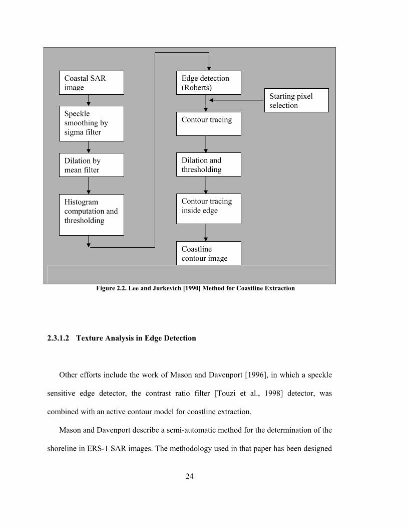
Another approach made by Lee and Jurkevich [1990], presents a coastline detection
method based in a series of operations described in general terms as follows:
Land/Water Boundary Enhancement
3x3 Median Filtering
Histogram Equalization
Thresholding
Contour following algorithm
7x7 Maximum Filter (dilation)

23
After performing 1) the speckle smoothing and filtering using an adaptative Lee
filter, 2) Sobel edge detection is applied. Once all the edges present in the image (land,
water and coastline) are obtained, 3) a 5x5 mean filter is applied more than one time,
dilating the edges to fill the gaps. The smoothed image is then 4) thresholded. Hence,
water-land separation is achieved. For this binary image, 5) Roberts edge detection is
computed, producing a thinner contour image ready to be traced with a clockwise
contour following algorithm.
The reason for applying Robert’s operator is that the edges generated are 1-pixel
wide, making the edge tracing more precise [Lee and Jurkevich, 1990].
Because the mean filter is applied twice, the detected coastline pixels are, on
average, six to eight pixels away from the original image coastline pixels.
To refine the coastline, a (5x5) mean filter is applied twice over the edge, followed
by a thresholding operation. Then, the coastline is retraced using the same algorithm, but
now only the inside edges are traced. After refinement, the new coastline matches that of
the original image to within a pixel or two.
Because the mean filter is applied more than once, before refinement, the land-water
boundary is also affected producing an offset of approximately six to eight pixels away
from the original image coastline pixels [Lee and Jurkevich, 1990].
They achieved reasonable positional accuracy using their method, but state that
refinements are necessary to achieve the accuracy required for geographical mapping.
However, this methodology cannot solve the problem regarding environmental noise.
So, in the application of the contour-following algorithm, the operator must achieve
image interpretation to avoid the delineation of contours over noisy areas.
24
Figure 2.2. Lee and Jurkevich [1990] Method for Coastline Extraction
2.3.1.2 Texture Analysis in Edge Detection
Other efforts include the work of Mason and Davenport [1996], in which a speckle
sensitive edge detector, the contrast ratio filter [Touzi et al., 1998] detector, was
combined with an active contour model for coastline extraction.
Mason and Davenport describe a semi-automatic method for the determination of the
shoreline in ERS-1 SAR images. The methodology used in that paper has been designed
Coastal SAR image
Speckle smoothing by sigma filter
Dilation by mean filter
Histogram computation and thresholding
Edge detection (Roberts)
Contour tracing
Dilation and thresholding
Contour tracing inside edge
Starting pixel selection
Coastline contour image

25
for the use in the construction of a digital elevation model (DEM) of an intertidal zone
using a combination of remote sensing and hydrodynamic modeling techniques.
The Mason and Davenport method is a coarse-to fine processing approach, in which
sea regions are first detected as regions of low edge density in a low resolution image.
They use a sequence of image processing algorithms. The procedure starts by finding a
rough division between land and sea (note the concept of land-water enhancement) in a
coarse resolution processing stage. This rough sea-land segmentation is shown in the left
part of the workflow in Figure 2.4. After that, the SAR sub-image areas near the
shoreline are processed at high resolution using an active contour model algorithm. This
procedure is shown in the right part of Figure 2.4.
This procedure also achieves good results over areas without excessive noise. More
than 90% of the shoreline detected by this methodology appears visually correct [Mason
and Davenport, 1996]. However, this method fails when texture in sea backscatter is
similar to some portions of land.

26
Figure 2.3. Mason and Davenport [1996] Method for Coastline Extraction
SAR image
Reduce image by averaging
Construct edge density image
Determine thresholded texture edges
Segment regions in texture image
Select sea regions
Merge small regions
Generate rectangles along land-sea boundaries
SAR sub-image
Threshold edges
Segment sea region using active contour modeling
Find land-sea boundary segments
Refine boundary segments positions in full image
Detect edges

27
2.3.2 Shoreline Extraction using Polarimetric SAR Images
Polarimetric images have been recognized as having stronger power to discriminate
between different terrain covers than is possible with a single polarization SAR image.
Besides the shoreline detection in polarimetric SAR images using traditional
classification techniques, Yu and Acton [2004] presented another approach (see Figure
2.4).
They apply first a polarimetric filter to yield a single, speckle reduced base image.
Primary edge information is then derived by Instantaneous Coefficient of Variation
(ICOV) operator from a Speckle Reducing Ansiotropic Diffusion (SRAD) processed
base image. SRAD is used to enhance edges in the base image and further reduce
speckle noise in the image. Next, the resulting edge image is parsed by a watershed
segmentation algorithm, which partitions the image scene into a set of disjoint segments.
Region merging is performed to eliminate subscale segments. By adopting a region
adjacency graph (RAG) representation for segments and calculating a similarity metric
from the radar brightness (not texture) for each pair of adjacent regions, the region pairs
with high similarity are merged iteratively until a desired result is achieved, eliminating
the undesired boundary segments while delineating the coastlines correctly [Yu and
Acton, 2004].
This procedure gives better results than Lee and Jurkevich or Mason and Davenport
methods [Yu and Acton, 2004]. However, because this procedure is based in segments,
it fails in the identification of small islands, especially when noisy images are used.

28
Figure 2.4. Yu and Acton Method [2004] for Coastline Extraction
2.3.3 Shoreline Detection in the Frequency Domain
The edge detector achieved by Niedermeier et al. [1999] consists of three parts. A first
guess part leads to a coarse land-water determination, based on the fact that wavelet
based edge detector enhances strong edges over land areas and only weak edges over
sea. From this, a thresholding and a so-called blocktracing are performed yielding a
Edge detection by the ICOV
Pre-filtering speckle by polarimetric filtering
Edge image enhancement by SRAD
Pre-filtering speckle
Watershed transform of the ICOV image
Solving over segmentation by region merging
Coastline Extraction
Similarity metric for region merging

29
rough segmentation into water, land and small coastal area in between. Figure 2.5
outlines the principal steps.
Figure 2.5. Niedermeier [1999] Method for Coastline Extraction
SAR image
Wavelet decomposition
Thresholding
Blocktracing
Edge selection
Scale propagation
Active contour
Continuous coastline

30
In a refinement step the full resolution edge is detected in the coastal region. Due to
wavelet theory its localization gets better using scale propagation. As a final step,
individual edge segments are connected to a continuous shoreline using a snake
algorithm.
The wavelet-based edge detector algorithm seems to be a suitable choice for
extracting coastlines from SAR images. The separation of edges from noise is achieved
by thresholding the resulting image after filtered with wavelet. However, this threshold
operation fails when it is applied to edges detected over strong and local rough surface
areas.
2.4 Summary
After introducing brief concepts regarding the different representations for a SAR
image, this chapter described some of the previous works achieved in coastline detection
using amplitude images, which generally are based in land-water separation procedures
with the further application of a contour following algorithm.
Previous work describes the extraction of coastline using algorithms in the spatial
domain. Also, some work has been done in the frequency domain using wavelet
transform to detect the edges and the use of active contours method to extract the
shoreline. However, the main problem regarding the rough sea surface caused by strong
wind cannot be easily solved because “wind-forced” noise is local and its gray level
value can be easily higher than pixel values in some areas in land.
31
The techniques described here give good results in the extraction of shorelines over
relatively environmental noise-free areas. In that way, most of these previous works
have been achieved in areas where the texture of the sea pixels are homogeneous and
well differentiated from land pixels. Consequently, they still present some problems if
applied in areas with local sea roughness. This problem is solved in this thesis by the use
of the Multitemporal Segmentation Method.

32
Chapter 3
INHERENT PROBLEMS ENCOUNTERED USING AMPLITUDE IMAGES
3.1 Background
Because this research is based in the extraction of coastline using single amplitude
SAR images, a brief description regarding SAR images is outlined in this chapter.
Radar concepts differ from optical theory both in geometry and in the kind of
information received. Images provided by optical sensors contain information about the
surface layer of the imaged objects (i.e., color), while microwave images provide
information about the geometric and dielectric properties of the surface or volume
studied (i.e., roughness)[European Space Agency, 2004].
When seeking the land-water separation, inherent distortions and noise present in
radar images are responsible for most problems in the automatic or semi-automatic
features detection. Hence, accurate shoreline position is hard to achieve by extracting
land-water boundaries by edge detection and edge-tracing algorithms.
3.2 Radar Geometry

33
Remote sensing image data in the microwave range of wavelengths is generally
gathered using the technique of side-looking radar. A pulse of electrical energy at the
microwave frequency (or wavelength) of interest is radiated to the side of the aircraft (or
spaceborne) at an incidence angle [Richards and Jia, 1999].
The platform is flying in its orbit and carries a SAR sensor, which points
perpendicular to the flight direction. The projection of the orbit down to Earth is known
as the ground track or subsatellite track. The area continuously imaged from the radar
beam is called radar swath. In the case of ERS, due to the look angle of about 23
degrees, the imaged area is located some 250 km to the right of the subsatellite track.
The radar swath itself is divided in a near range (i.e. the part closer to the ground track)
and a far range [European Space Agency, 2004]. Figure 3.1 shows the general diagram
of the image acquisition in radar geometry.
In SAR images, the direction of the satellite's movement is called azimuth direction,
while the imaging direction is called range direction. The SAR measures the power of
the reflected signal, which determines the brightness of each picture element (pixel) in
the image.

34
Figure 3.1. Geometric Configuration of SAR Images [European Space Agency, 2004]
The returning signal is based in the backscatter properties of the material where the
signal is reflected. Different surface features exhibit different scattering characteristics:
- Urban areas: very strong backscatter.
- Forest: medium backscatter.
- Calm water: smooth surface, low backscatter.
- Rough sea: increased backscatter caused by wind and current effects. This effect is
very important for hydrographic applications and coastal mapping. This problem is the
main issue in this thesis and it is solved with the method proposed.

35
Also, there are two kinds of data display, as shown in Figure 3.2:
- Slant range image, in which distances are measured between the antenna and the
target.
- Ground range image, in which distances are measured between the platform ground
track and the target, and placed in the correct position on the chosen reference plane.
From an image production viewpoint, the slant range resolution is not of interest. Rather
it is the projection of this onto the horizontal plane as ground range resolution that is of
value for the user. Slant range data is the natural result of radar range measurements.
Figure 3.2. Slant and Ground Range Geometry during the Image Acquisition [European Space Agency, 2004]

36
Transformation to ground range requires correction at each data point for local
terrain slope and elevation. Geometric distortions are one of the most important
constrains in radar images and they must be corrected to achieve the final product.
3.2.1 Radar Distortions in Amplitude Images
The geometric distortions present on a radar image can be divided into:
- Range distortions: Radar measures slant ranges but, for an image to represent the
surface correctly, it must be ground range corrected.
- Elevation distortions: This occurs in those cases where points have an elevation
different from the mean terrain elevation.
Both kinds of distortions produce different kinds of effects in the image. These
effects are shown in Figure 3.3.
Probably the most striking feature in SAR images is the "strange" geometry in range
direction. The SAR imaging principle causes this effect: measuring signal travel time
and not angles as optical systems do. The time delay between the radar echoes received
from two different points determines their relative distance in the image. Because of this
signal travel time measurement, different distortions can happen to the radar images in
the range direction, depending also on the terrain elevation.

37
3.2.1.1 Foreshortening
Foreshortening is a dominant effect in SAR images of mountainous areas. Especially
in the case of steep-looking spaceborne sensors, the across-track slant-range differences
between two points located on foreslopes of mountains are smaller than they would be in
flat areas. This effect results in an across-track compression of the radiometric
information backscattered from foreslope areas. To solve this, the image must be
compensated during the geocoding process if a terrain model is available.
Foreshortening is obvious in mountainous areas, where the mountains seem to "lean"
towards the sensor. It is worth noting that foreshortening effects are still present on
ellipsoid corrected data.
3.2.1.2 Layover
If, in the case of a very steep slope, targets in the valley have a larger slant range
than related mountaintops, then the foreslope is "reversed" in the slant range image.
This phenomenon is called layover: the ordering of surface elements on the radar image
is the reverse of the ordering on the ground. Generally, these layover zones, facing radar
illumination, appear as bright features on the image due to the low incidence angle.
Ambiguity occurs between targets hidden in the valley and in the foreland of the
mountain, in cases where they have the same slant-range distance. For steep incidence
angles this might also include targets on the back slope.

38
Geocoding can not resolve the ambiguities due to the representation of several points
on the ground by one single point on the image; these zones also appear bright on the
geocoded image.
3.2.1.3 Shadowing
A slope away from the radar illumination with an angle that is steeper than the
sensor depression angle provokes radar shadows.
Figure 3.3. Radar Distortions caused by the Slant Range Geometry and the Terrain Elevation [The Alaska Satellite Facility, 2004]

39
It should be also noted that the radar shadows of two objects of the same height are
longer in the far range than in the near range. Shadow regions appear as dark (zero signal
or pixel value) with any changes due solely to system noise, sidelobes, and other effects
normally of small importance.
3.3 Geographic Characteristics and the Incidence Angle
Based upon the previous considerations on SAR image geometry, the following
remarks can be formulated in order to assist the interpreter (from ESA webpage):
- For regions of low relief, larger incidence angles give a slight enhancement to
topographic features. So does a very small incidence angle.
- For regions of high relief, layover is minimized and shadowing exaggerated by
larger incidence angles. Smaller incidence angles are preferable to avoid shadowing.
- Intermediate incidence angles correspond to low relief distortion and good detection
of land (but not water) features.
- Small incidence angles are necessary to give acceptable levels of backscattering
from ocean surfaces.
- Planimetric applications need the use of ground range data, which usually requires
the use of digital elevation data and image transformation.
3.4 Spatial Resolution

40
In images, the spatial resolution is described by the pixel size [Richards and Jia, 1999].
Even more fundamental, at least two pixels are required to represent each resolution cell,
which is a consequence of spatial sampling rules.
Spatial resolution is the most important parameter to discriminate features like
objects or edges. In the case of coastal mapping, the discrimination between land and
water in coastal zones is an important problem to solve, and it is directly related to
spatial resolution as well as radiometric resolution or intensity levels in the case of radar
images.
By convention, pixel size in SAR imagery is chosen to conform to standard map
scales hence, it must be a discrete multiple (or divisor) of 100 metres. For example,
ERS-1 data, having nominal resolution of 28 metres in range and azimuth, is delivered
with 12.5 metre pixel spacing.
This means that rocks smaller than 12.5 metres cannot be detected using these kinds
of images. Consequently, this consideration must be taken into account regarding the
application of the generated coastline.
2.5 Summary
Radar images have inherent problems due their special configuration, which will
cause differences in backscatter or shadowing effects. These detrimental effects will
affect the achievement of an efficient procedure to achieve land-water separation. The

41
low-level pixel value from shadow areas can be usually less than the pixel values from
the sea surface.

42
Chapter 4
TESTING BASIC OPERATIONS FOR LAND-WATER SEPARATION IN SAR
IMAGES
4.1 Introduction
This chapter presents a combination of linear filters and morphological operations used
to enhance the land-water boundary, getting rid of the edges present over land, while
preserving the main edge consisting in the shoreline.
The general procedure most widely used to detect the shoreline is tested to obtain a
rough land-water separation in the analyzed areas. The application of morphological
operations will help to solve the offset caused by the application of large smoothing
filters.
The area analyzed has a high backscatter on the sea surface; therefore, this chapter tests
the results after using common filters for land-water separation.
4.2 Existing Filters usable for Land-Water Separation
From previous works done in coastline detection it was possible to identify the main
concepts applied that achieved acceptable results. These concepts are: reduction of

43
noise, land-water enhancement and edge detection. Also, the use of a contour-following
algorithm is widely applied in most of them. The same main concepts are applied in this
chapter. In general terms, land water enhancement is achieved using basic operations.
As shown in Figure 4.1, to extract information from radar images, first, an adequate
process of filtering the image to eliminate speckle must be achieved without losing
spatial resolution. Then, the procedure for the enhancement of water-land boundary is
very important to roughly determine the shoreline.
Figure 4.1. Coastline Detection Methodology using Most Common Filters
EDGE DETECTION
3X3 LEE (SIGMA) FILTER (TWICE)
HISTOGRAM SCALING 16-BIT TO 8-BIT
EDGE ENHANCEMENT IN THE IMAGE
SMOOTHING FILTER AND GRAY LEVEL OPENING
LAND-WATER ENHANCEMENT
NOISE REDUCTION
3X3 MEDIAN FILTER
SEGMENTATION
CONTOUR FOLLOWING ALGORITHM AND REFINEMENT
ROBERTS FILTER
SOBEL EDGE DETECTOR

44
4.2.1 Noise Reduction in SAR Images
Speckle noise is a multiplicative process that is the primary source of corruption in
coherently illuminated imaging modalities including synthetic aperture radar [Schultze
and Wu, 1995]. This is caused by the random constructive and destructive interference
of the de-phased, but coherent return waves scattered by the elementary scatterers within
each resolution cell [Xiao et al, 2003]. A complete description of speckle is in
Henderson and Lewis [1998].
Most commonly used speckle filters have good speckle-smoothing capabilities.
However, the resulting images are subject to degradation of spatial and radiometric
resolution, which can result in the loss of image information. The amount of speckle
reduction desired must be balanced with the amount of detail required for the spatial
scale and the nature of the particular application [Xiao et al, 2003].
Most of these algorithms are based on smoothing the image while preserving the
features present in it. Particularly, SAR images assume a multiplicative noise. Described
by Lee and Jurkevich [1990], the basic relation of this model is given by the equation
4.1.
zi,j = xi,j vi,j and vi,j ~ (1,σ 2) Equation 4.1
Where zi,j is the gray level of the observed SAR pixel, xi,j is its ideal or noise-free
counterpart, and vi,j is the noise characterized by a distribution with mean equal to one
and variance σ 2. This assumed statistical model for noise could vary according to the

45
different existing approaches to smooth the speckle noise without degrading the
sharpness of the major edges in the image.
Much work has been done on speckle filtering of SAR imagery. Filtering techniques
can be grouped into multi-look processing and posterior speckle filtering techniques
[Xiao et al, 2003].
Multi-look techniques have the disadvantage that the greater the number of views
used to filter the image, the smoother the processed image while losing spatial
resolution. To avoid that, many posterior techniques have been developed to further
reduce speckle. They are based on either the spatial or the frequency domain. Adaptive
filters based on the spatial domain are more widely used than frequency domain filters.
Most frequently used adaptive filters including Lee and Frost assume a Gaussian
distribution for the speckle noise, while the Gamma filter assumes a gamma distribution.
Good results over SAR images can be achieved using the Frost Filter or Lee filter,
using a number of looks equal to four and using a 5x5 window.
Others less frequently used filters are the mean filter (to smooth the image) and the
median filter. The last one has the advantage that smoothes the image while preserving
the edges [Richards and Jia, 1999].
In general, there were no big differences between the set of speckle reduction filters.
However, because of the problem of backscatter over sea surface, a good approach was
using the selected filter more than once to minimize the speckle associated and the
bright return from rough water or other matters in a predominantly dark part of the
image [Erteza, 1998]. Using median filter, a 3x3 or 5x5 windows is good enough to
remove those single points whose values are out of line with neighboring pixels. Figures

46
4.2a) to 4.2d) show some results after applying existing SAR speckle filters. From all the
tested filters, the Lee filter was selected to smooth the speckle over the analyzed images.
a) The study area before applying filters.
b) Median filter 5 x 5.
c) Gamma filter 5 x 5, looks 4, combined with
edge sharpening filter. d) Lee filter 3x3 applied twice.
Figure 4.2. Different Filters used for Speckle Reduction
4.2.2 Enhancement of Land-Water Boundary
Separation between land and water is the most important step in the coastline
extraction procedure. The first step, reduction of noise, is intended to minimize variation

47
within pixels of land and within pixels of water, while maintaining the distinct
characteristics for each.
Edge enhancement is a way of increasing geometric detail in an image, considering
that an edge is the boundary between an object and the background [Parker, 1997]. In
this case, land and water are considered objects and background respectively. All lines
or edges have a direction such that one side is always brighter than the other [Zelek,
1990].
Because the coastline is the most important feature in this image, enhancement of the
land-water boundary is a necessary task. The most commonly used procedure is
histogram equalization to increase the contrast throughout the image. Another method to
modify and spread the histogram of gray level values is transforming the image from
unsigned 16-bit to 8-bit. Then the old 65,536 different gray values image is now
transformed to 256 gray levels. Even when this elemental operation changes the digital
number of pixels, it is well suited to enhance the contrast between land and water. The
histogram scaling produces a lack of radiometric resolution that is detrimental to detect
features in land. That effect has no importance because the main purpose is the coastline
enhancement and no land analysis is being performed.
4.2.2.1 Most used Edge Detection and Enhancement Techniques
4.2.2.1.1 Edge Detection

48
Edge detection is the process of locating the edge pixels. An edge enhancement will
increase the contrast between the edges and the background in such a way that edges
become more visible [Parker, 1997]. In addition, edge tracing is the process of following
the edges, usually collecting the edge pixels into a list [Martin and Tosunoglu, n.d.].
Usually an edge can be modeled as a step or as a ramp. In the “real world” edges
change gradually over the images, so the ramp is the best one to fit. There are three
economically different techniques to detect edges over an image [Richards and Jia,
1999]. The most commonly used algorithms from these techniques are used in this
research.
4.2.2.1.1.1 Derivative Operators
The rate of change of a function, and the rate of change of grey levels in an image is
large near an edge and small in relatively constant areas [Parker, 1997]. The gradient
vector can be applied (partial derivative in x and y direction) in a discrete way,
calculating the differences in grey levels over some local region.
Λx1 A(x ,y) = A(x + 1,y) – A(x - 1, y)
Λy1 A(x,y) = A(x,y + 1) – A(x, y - 1) Equation 4.2
Then, the magnitude is calculated, that will give the strength of the edge:

49
∂∂
+
∂∂
=22
yA
xAGmag = ( )yx 22 ∇+∇ Equation 4.3
Direction of the edge:
∇∇
= −
yxGdir 1tan Equation. 4.4
Then, if the resulting gradient exceeds threshold, the edge is detected, otherwise will
not be detected.
4.2.2.1.1.2 The Roberts Edge Detector
For digital image data in which x and y are “discretized”, the continuous derivatives
are replaced by differences [Richards and Jia, 1999].
Λ1 = A(x ,y)- A(x + 1,y + 1)
Λ2 = A(x + 1,y) – A(x, y + 1) Equation 4.5
They constitute the discrete components of the vector derivative at the point x + ½, y +
½, in the diagonal directions. Hence both horizontal and vertical edges are detected, as
will be diagonal edges. Since this procedure computes a local gradient it is necessary to
choose a threshold value above which edge gradients are said to occur.

50
4.2.2.1.1.3 The Sobel Operator
Sobel computes discrete gradient in the horizontal and vertical directions at the pixel
location x,y.
It is more costly to evaluate than the Roberts filter. The orthogonal components of
the gradient are:
Equation 4.6
Λ1 = {A(x-1 ,y+1) - 2A(x-1,y) + A(x–1, y–1)}- {A(x+1 ,y+1) - 2A(x+1,y) + A(x+1, y–1)}
Λ2 = {A(x-1 ,y+1) - 2A(x, y+1) + A(x+1 ,y+1)}- {A(x-1 ,y-1) - 2A(x,y-1) + A(x+1, y–1)}
Hence, horizontal and vertical as well diagonal edges are detected. As before, a
threshold on the responses is generally chosen to allow an edge map to be produced in
which small responses, resulting from noise or minor gradients, are suppressed.
4.2.2.1.1.4 Edge Detecting Templates
Template operators are used not only for smoothing and enhancement, but also for
line and edge detection. A template is a box or window previously defined and moved
over the image row-by-row and column-by-column. In general terms, the product of the
pixel brightness values, covered by the template at a particular position and the template
entries are summed to give the template response. This response is then used to define a
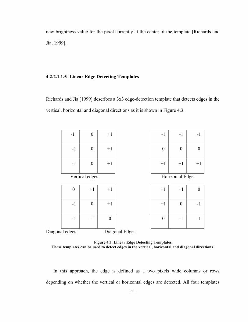
51
new brightness value for the pixel currently at the center of the template [Richards and
Jia, 1999].
4.2.2.1.1.5 Linear Edge Detecting Templates
Richards and Jia [1999] describes a 3x3 edge-detection template that detects edges in the
vertical, horizontal and diagonal directions as it is shown in Figure 4.3.
-1 0 +1 -1 -1 -1
-1 0 +1 0 0 0
-1 0 +1 +1 +1 +1
Vertical edges Horizontal Edges
0 +1 +1 +1 +1 0
-1 0 +1 +1 0 -1
-1 -1 0 0 -1 -1
Diagonal edges Diagonal Edges
Figure 4.3. Linear Edge Detecting Templates These templates can be used to detect edges in the vertical, horizontal and diagonal directions.
In this approach, the edge is defined as a two pixels wide columns or rows
depending on whether the vertical or horizontal edges are detected. All four templates

52
must be applied to obtain edges in all orientations, using a threshold to determine the
edge map. If the threshold is too low it will lead to many false edge counts. On the other
hand, if the threshold is too high, little discontinuities will appear on the detected edge.
4.2.2.1.1.6 Sobel Template
As specified before, the Sobel edge detector is a derivative-based operator that is
used in templates form for computational purposes. The purpose is to use a small
discrete template as a model instead of using a derivative operator [Parker, 1997]. In
other words, it is a spatial derivative technique but reduced to templates. Here, the
following templates are used in the form of convolution mask, locating the resulting
pixel value in the center of the template in the output image.
Kernels in Figure 4.4 are designed to respond maximally to edges running vertically
and horizontally related to the pixel grid. After calculation, the resulting image is
thresholded. All pixels will have some responses to templates but the very large
responses will correspond to an edge.

53
Sx Sy
1 0 1 1 2 1
-2 0 2 0 0 0
-1 0 1 -1 -2 -1
Vertical Edges Horizontal Edges
Figure 4.4. Sobel Templates These templates can be used to detect edges in the vertical and horizontal directions.
4.2.2.1.2 Edge Enhancement
Edge enhancement is a particularly simple and effective means for increasing
geometric detail in an image. First edges are detected and then they are either added
back into the original image to increase contrast in the vicinity of an edge, or the edges
are highlighted using saturated (black, white or colour) overlays on borders [Richards
and Jia, 1999]. If the edges are added back into the original image in varying
proportions, the boundaries are enhanced.
Land-water enhancement is one of the most important steps to achieve a good
segmentation between them, and further coastline delineation.
4.2.3 Testing Existing Techniques for Shoreline Enhancement

54
After histogram scaling, the next step is to eliminate edges in land, keeping the
coastline edge with minimum changes. In the spatial domain, another important step is
focused on getting rid of the edges present in land, while preserving the main edge,
which consists of the shoreline.
Previous works in coastline detection use similar techniques that focus on the
enhancement of land-water boundary.
4.2.3.1 Edge Detection Focusing on the Shoreline
This chapter presents a combination of linear filters and morphological operations
used to enhance the land-water boundary, getting rid of the edges present in land, while
preserving the main edge consisting in the shoreline.
After scaling the image from 16 bits to 8-bits, some pixels have high gray-level values if
compared with its neighbors. Because that, a median filter 3x3 window is applied to
smooth the image while enhancing the edges.
Although all the edges present in the image can be detected using any edge detector
method, using the Sobel filter to detect all the edges gives good results, because using a
3x3 window the detected edges are strong and consistent.
Because the new pixel values in the Sobel image correspond to the rate of change
between neighboring pixel values in the original image, the resulting histogram from
Sobel shows low gray level values in the areas with a low rate of change (most of the
image data), and high gray level values in the edges, being even higher in those
55
prominent edges (i.e. shoreline). Figure 4.5 shows the corresponding histograms with
gray-level values obtained from the original image (left) and the histogram obtained
from the resulting image after Sobel edge detector is applied (right).
Figure 4.5. Histograms of the Original Image and its Respective Sobel Image
After the edge detection stage, edge enhancement is applied using different proportions. From
testing different combinations, it was found that 30% of the pixel value obtained using Sobel
added to 70% of the pixel value from the original image produced the best results. Figure 4.6
shows the effect of this operation focusing on the enhancement of the land-water boundary
while avoiding the influences of other edges present in land. The resulting image once 30% of
the pixel value obtained using Sobel is added to the 70% of the pixel value from the original
image. The left image shows the resulting image and the right image shows the corresponding
grey-level values histogram.

56
Figure 4.6. Enhanced Image and its Respective Histogram
Using this technique, the grey-level value of the pixels on land is decreased and
made more homogeneous. The application of this technique produces a steeper land-
water separation.
4.2.3.2 Texture Analysis Focusing on Shoreline
In another approach, the Sobel edge detector applied in the land-water enhancement
step was replaced by texture analysis using different parameters. A set of texture
measurements is calculated for all pixels in an input image.

57
4.2.3.2.1 Texture
Texture can be defined as a repetition of a pattern over a region. Texture is an
important issue to be analyzed in radar images. Texture is studied to perform
segmentation, where the result could be an image in which texture has been replaced by
a unique grey level or color. The following sections describe different approaches to
measure texture [Parker, 1997].
4.2.3.2.1.1 Statistics
A region can be identified using its particular texture. This method is based in the
use of small windows W x W pixels to capture samples of the particular properties over
an area. The window moves over the image calculating the following parameters for
each case separately.
4.2.3.2.1.1.1 Mean Windows
The use of average grey level is not recommended to distinguish between textures
[Parker, 1997]. Average windows are usually used to blurr the image. As a result of the
moving window, the boundary between textured regions can only be determined within

58
a distance of about W pixels, where W is the width of the window. Each pixel in the
image is replaced by the average of the levels seen in a region W x W pixels in size
centered at that pixel. Then, thresholding the image into two regions using the new
average levels proceeds. Boundary regions (exact location) depend on the threshold that
is applied to the mean-level image.
4.2.3.2.1.1.2 Standard Deviation Windows
Standard Deviation Windows work better than mean windows [Parker, 1997]. It is
more consistent in the changes in levels than is in the levels themselves. After
calculating the mean of each window, the standard deviation of each pixel is calculated
with respect to the mean. The resulting value is displayed in the center of the window.
The formula is shown in Equation 4.7.
( )N
xxMn
n∑ −= Equation 4.7
4.2.3.2.1.2 Gray – Level Co-occurrence Matrices (GLCM)
Statistical windows are easy to calculate but it do not provide any information about
the repeating nature of texture. Gray Level Co-occurrence Matrices (GLCM) contains

59
information about the positions of pixels having similar grey level values. They attempt
to capture directionality of patterns. The idea is to scan the image and keep track of how
often pixels that differ by a specified amount in value are separated by a fixed distance
in “d” position.
Directionality is determined by using multiple matrices, each one for each direction
of interest. Then, the matrix, associating them to texture, captures distance and direction.
Therefore, for every value of “d”, we have 4 images (horizontal, vertical and two
diagonal) each of which is 256 x 256 for an original image with 256 levels of gray.
However, this procedure produces an enormous amount of data. To minimize data, a few
simple numerical values called descriptors are calculated to encapsulate the information.
In other words, the grey –level difference between pixels in a given direction is recorded
in a small window of the original image. Those descriptors could be represented by
statistical moments defined before and others descriptors such as maximum probability,
contrast, homogeneity and entropy. After the descriptor is calculated, it is placed at
current pixel’s position in the output image.
4.2.3.2.1.2.1 Edge Detection using GLCM Variance Windows
The measurements are based on second-order statistics computed from the grey level
co-occurrence matrices. Either texture measures for a specific direction or directional
invariant measures can be computed. After testing different parameters for texture

60
analysis, it was found that variance acted better to detect edges. Therefore, this
parameter was used to analyze the texure in the image.
Figure 4.7 shows the effects of applying texture analysis during the enhancement of
land-water boundary and a comparison between Sobel (left) and texture analysis using
variance (right) in the detection of all the edges present in the image. Below each
picture, its respective histogram shows the grey level distribution. Grey level pixels in
the texture image are too high, causing problems for further operations.
Visually, the resulting image after texture using variance windows acted similar to
the images treated with the Sobel edge detector, however the implementation of this
procedure implies more computational cost. Therefore, Sobel operator was finally
chosen to detect the edges in the land-water enhancement process.
However, after using Sobel and adding the 70% of image back to contrast coastline
boundary (Figure 4.6), there are still some undesirable edges in land close to the
coastline that should be eliminated without modifying the shoreline.

61
Figure 4.7. Sobel and Texture (Variance) Images

62
4.2.4 Existing Techniques used to Reduce the Unnecessary Edges
4.2.4.1 The use of Smoothing Filters
To get rid of the undesirable edges, the image is smoothed using a 5x5 mean
window. Larger windows will be detrimental, and will produce large offsets in the
shorelines. To avoid this effect, this smoothing window is applied just once. After the
application of the smoothing window, digital morphology can be used to reduce the
unnecessary edges.
4.2.4.2 The use of Digital Morphology
After smoothing the image, a gray level opening operation is performed using a 3x3
window. In gray level images, the opening operation (gray-scale erosion followed by
gray-scale dilation) is a smoothing operation that decreases the average pixels value.
Digital morphology is a way to describe or analyze the shape (the form and structure
of an object) of a digital (raster) object. In an image, pixels are organized into groups
having a two-dimensional structure called shape. A group of mathematical operations
can be applied to the set of pixels to enhance or highlight specific aspects of the shape so
that they can be counted or recognized [Martin and Tosunoglu, n.d.].
These different properties are inherent to morphological operations:
Being A and B a set of pixels,

63
- Translation: (A)x = {c | c = a + x, a ε A}
- Reflection: Â = {c | c = -a, a ε A}
- Union: A U B = {c| ((c ε A) or (c ε B))}
- Intersection: A ∩ B = {c | (c ε A) & (c ε B)
- Complement : Ac = {c | c ε A}
- Difference: A – B = A ∩ Bc
In this chapter, dilation and erosion, which are basics operations based in these
fundamental properties, are described as binary (bi-level) operations. In general, an
operator is defined as a set of black pixels with a specific location for each of its pixels
given by the pixel row and column indices [Parker, 1997].
4.2.4.2.1 Binary Dilation
Binary dilation can be defined as:
A +B = {c/c = a + b, a 0 A, b 0 A}
Where A represents the image to be transformed and B is a second set of pixels
called structure element, with a particular shape that acts on the pixels of A producing an
expected result. In Figure 4.8, the pixel marked with an x corresponds to the origin of
the image. Then, the structuring element is a template moving over the image, producing
the dilation. In general terms, dilation is a morphological operation to make the object
wider by adding neighboring pixels at the boundaries in the directions specified by the

64
structuring element. In binary images, it can be implemented by marking all white pixels
having at least one black neighbor, and then setting all of the marked pixels to black
[Parker, 1997].
Structuring element
2nd dilation
3rd dilation
Figure 4.8. Effects of Dilation over the Original Image using a 3x3 Structuring Element
4.2.4.2.2 Binary Erosion
Binary erosion produces the inverse results obtained by the dilation operation, but
the procedure is slightly different from the inverse procedure of dilation. Erosion
corresponds to the set of pixels “c” such that the structuring element B translated by “c”
corresponds to a set of black pixels in A. As the result, any pixel that does not match the
pattern defined by the black pixel in the structuring element will not belong to the result.
Hence, erosion makes the object image smaller by removing the outer layer of pixels
from an object. This can be implemented by marking all black pixels having at least one
A
B

65
white neighbor, and then setting to white all of the marked pixels. Mathematical
operations differ between dilation and erosion, and those concepts can be applied either
to binary or gray level images.
4.2.4.2.3 Opening and Closing
The application of erosion followed immediately by dilation using the same
structuring elements is called opening. This binary operation attempts to open small gaps
between touching objects in an image [Martin and Tosunoglu, n.d.]. Also, it can be
explained as a process that destroys edges. This concept is directly applied to the
analyzed coastal image to get rid of the edges present in land while preserving the
coastline.
Also, the application of a dilation procedure immediately followed by erosion using
the same structuring element is called closing. As its name indicates, it closes or fills the
gaps between objects. Practically, closing is a process that joins edges. More information
regarding morphological operations can be found in Parker, 1997.
4.2.4.2.4 Application of Opening Filter to Reduce the Undesirable Edges
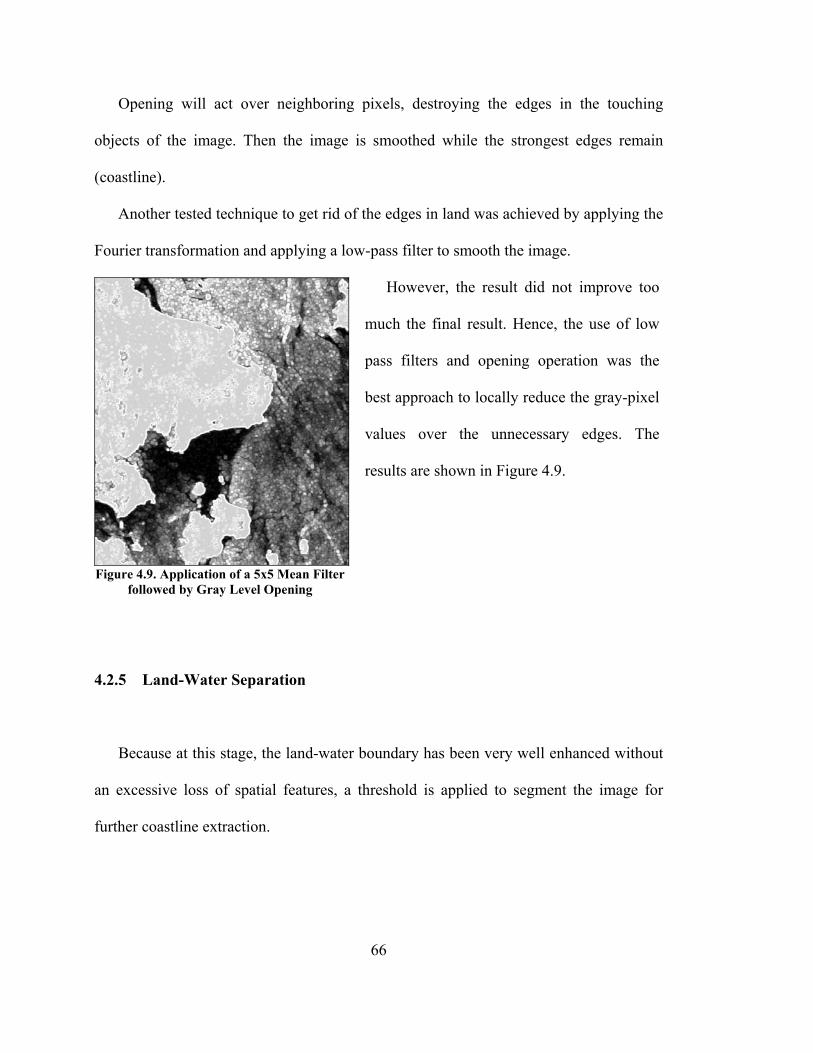
66
Opening will act over neighboring pixels, destroying the edges in the touching
objects of the image. Then the image is smoothed while the strongest edges remain
(coastline).
Another tested technique to get rid of the edges in land was achieved by applying the
Fourier transformation and applying a low-pass filter to smooth the image.
Figure 4.9. Application of a 5x5 Mean Filter
followed by Gray Level Opening
However, the result did not improve too
much the final result. Hence, the use of low
pass filters and opening operation was the
best approach to locally reduce the gray-pixel
values over the unnecessary edges. The
results are shown in Figure 4.9.
4.2.5 Land-Water Separation
Because at this stage, the land-water boundary has been very well enhanced without
an excessive loss of spatial features, a threshold is applied to segment the image for
further coastline extraction.

67
4.2.5.1 Grey-Level Segmentation or Threshold
Gray Level Segmentation is a conversion between a gray-level image and a bi-level
image. Bi-level image is a monochrome image only composed of black and white pixels.
It should contain the most essential information of the image (i.e. number, position and
shape of objects), but is not comparable with the information offered by the grey-level
image [Martin and Tosunoglu, n.d.]. Pixels with similar gray levels in a nearby region
usually belong to the same object. By gray level segmentation we simplify many
recognition and classification procedures [Parker, 1997]. The most common procedure is
done by thresholding.
Thresholding is the procedure where all gray-level below this value will be classified
as black (0), and those above will be white (1).
Figure 4.10. Thresholding Operation used to Separate Object from Background
The most common way to choose the
threshold is by using the mean gray value in
the image, but it is not always useful,
especially when is used in a radar image
where the gray level values have a great
variability. However, in this case, because
the image is already processed, thresholding
by the mean value is well suited.

68
4.2.5.2 Application of Land-Water Segmentation
In real data, and especially in radar images, the object and background pixels have
overlapping gray level values.
In coastline extraction, is important to discriminate land from water. Because the
speckle and environmental noise, the simple use of segmentation techniques does not
work too well over radar images as is shown in Figure 4.11, where segmentation is
applied.
Figure 4.11. Application of a Single Threshold Operation to the Radar Image Even when the image was filtered to remove the speckle, there is no good land-water
discrimination.

69
The single use of segmentation is a bad approach, but combined with different
spatial procedures it should give acceptable results in land-water separation and finally
in coastline extraction.
The threshold must be carefully selected by the operator in order to remove
backscatter coming from the sea surface and to avoid missing land. In this case, the
critical areas in the image were examined.
The threshold used was the mean value of land pixels after the histogram was
computed (in this case was 179). Of course, the operator’s analysis is important here to
determine the value of threshold to be implemented. Figure 4.13a) shows the results of
the segmentation using that threshold. To eliminate noise from sea surface, four adjacent
pixels are considered for the connectivity. Each connected region, or segment, is given a
unique DN value in the output image.
After the whole process, the result of segmentation is poor. The noise over sea
surface is too high to achieve a proper land-water separation, and further coastline
detection. The problem is that there is still too much environmental noise close to the
shoreline in the original image, which will be misinterpreted with the shoreline itself.
Also in Figure 4.13b), the same problem is present over an image of the same area but
acquired at a different date.
Because of the noise problem, the coastline detection step cannot be achieved well
enough to obtain acceptable results.

70
a) Segmentation of image using a connectivity of
4 pixel neighbors. b) Segmentation of a second image using a
connectivity of 4 pixel neighbors. Figure 4.12. Results on Segmentation using Single SAR Images
4.3 Summary
In this chapter, rough land-water segmentation was achieved using the most common
procedure based in essential operations focused on the enhancement of the land-water
boundary and the reduction of grey-level value in the unnecessary edges, while keeping
the most important edge: the shoreline.
However, the results were not good. Hence, the high backscatter of rough sea surface
proved to be a problem that needs to be solved using a different approach.
71
Chapter 5
DEVELOPMENT OF A NEW METHOD FOR LAND-WATER SEPARATION
5.1 Introduction
The principal problem encountered in chapter four was caused by the presence of
rough sea surface due to wind conditions at the time of image acquisition. The
backscatter from that rough sea surface can usually equal or exceed the backscatter from
a portion of land close to the coastline, resulting in a detrimental factor to achieve land-
water separation.
To solve this problem this research uses two images from the same areas, but
acquired in different time. Certainly, one of those two images will present better sea
surface conditions than the other.
This chapter presents a novel methodology based on operations between
multitemporal images to enhance the input image to the point that backscatter over sea is
reduced to a point where it is so far below that from land that the differences are useful
in discriminating shoreline.
After that, the application of an iterative use of windows designed both to delete the
noise and to fill some undesirable gaps caused by shadowing is presented.

72
5.2 Data Used and Methodology Selected in this Research
The data used was The ERS - SAR Precision Image product, which is well suited for
quantitative analysis, photo-interpreting and image processing. Also, multitemporal
series are well suited using this product.
ERS-1 SAR looks at the Earth surface with a 23° incidence angle. Due to this,
images contain almost no shadow but may contain a large amount of layover and
foreshortening. The reduction of shadows is fundamental if the coastline to be extracted
is part of a high relief area, such as the area analyzed. Appendix II shows the main
characteristics of this product.
The developed methodology is based in two stages:
- A rough land water segmentation stage, which was presented in the previous
chapter. However, the use of multitemporal images now improves the land-water
segmentation.
- A refinement stage using the Multitemporal Segmentation Method and the
iterative use of windows to delete the noise, which is proposed in this chapter.
5.3 The Multitemporal Analysis for Noise Reduction
The multitemporal analysis consists in making image-image mathematical or
statistical operations to reduce the pixel values of those areas with high backscatter on
sea surface, especially when it is close to the shoreline. Hence, the problem is solved in

73
some locations of the first image and other locations for the second image. Most
researchers could think that just choosing the better image will solve the problem of
shoreline extraction, but because the noise coming over the sea surface is random and it
presents different characteristics in shape and location, this method certainly helps to
eliminate part of the high backscatter coming from sea surface.
To do image-image operations, both images must have the same reference system.
First, image-image registration is achieved, using the geocoded reference image or
entering manually the coordinates. The RMS has to be low, to ensure a good
registration, and care must be taken in the resampling mode (usually cubic convolution
used) and the channel used in the input and output. The user has to avoid making
changes in the digital value of the original pixels after this operation.
To avoid displacement over analyzed areas, both images must be subseted in a way
with both of them starting at the same pixel.
5.3.1 Averaging the Images
Averaging both images reduces the random noise over the sea surface; especially
when that noise is high close the coastline. To obtain the average of those images this
project uses the program called “8bits_imgavg.dsw”, modified from an existing C source
code to open and display LAN images1. To do that, Microsoft Visual C++ was used.
1 The original code to display images was provided by my supervisor, Dr. Yun Zhang

74
Figure 5.1 shows the original images where the images acquired on different time
present problems in some areas close to the shoreline, due the effect of wind. The left
image was obtained on 03 Nov 1995, and the right on 25 Nov 1992. Figure 5.2 shows
the effect of averaging the pixel value between two images, where the corresponding
averaged image solves the problem of random noise close to the shoreline over sea
surface. The averaging operation was performed after image scaling to 8bit.
Figure 5.1. Multitemporal Images
The same procedure was made over different areas, obtaining good results in the
land water boundary separation. The random noise over sea surface is solved using this
image-image operation. After doing this operation between multitemporal images, the

75
algorithm described in this chapter can be applied over the image, improving the
operations for land-water enhancement.
Figure 5.2. Result in Averaging two Images
5.3.2 Principal Components Analysis (PCA)

76
The multispectral or vector character of most remote sensing image data renders it
amenable to spectral transformations that generate new sets of image components or
bands [Richards and Jia, 1999]. These components then represent an alternative
description of the data, in which the new components of a pixel vector are related to its
old brightness values in the original set of spectral bands via linear operation [Richards
and Jia, 1999].
The most common way to use multispectral transformation is using satellite images
containing multiple channels to acquire the data in different wavelengths each one. The
multispectral or multidimensional nature of remote sensing image data can be
accommodated by constructing a vector space with as many axes or dimensions as there
are spectral components associated with each pixel [Richards and Jia, 1999].
Each channel provides different dimension in the vector space, in which each pixel
can be associated. Vectors, whose components are the individual spectral responses in
each band, describe the position of pixel points in multispectral space [Richards and Jia,
1999].
The mean position of pixels in the space is defined by the expected value of the pixel
vector x, according to equation 5.1:
∑=
==K
kkx
kxm
1
1}{ξ Equation 5.1
Where m is the mean pixel vector and xk corresponds to the individual pixels vectors
of total number K; ξ is the expectation operator.

77
The main steps in a Principle Component Transformation are:
- Assembling the covariance matrix of the image to be transformed, using the following
formula in equation 5.2:
( )( )∑=
−−−
=ΣK
k
tkkx mxmx
K 111 Equation 5.2
- Determining the eigenvalues and eigenvectors of the covariance matrix. At this stage
the eigenvalues are used simply to assess the distribution of data variance over the
respective components.
- Forming the components using the eigenvectors of the covariance matrix as the
weighting coefficients.
By examining the covariance matrix between the output eigenchannels, we observe
that the most consistent data of the transformed image from the original bands is in the
first principal component PC1. Then PC2 and the rest are in the remaining PCs. In this
case, the last PC contains the data, which is not correlated (see Figure 5.3).
The practical benefits of this application are:
- User can analyze any of the principal components individually or in combination as
a false color composite.
- Relationships between groups of pixels representing different land cover types might
become clearer if they are viewed in the principal axis reference system rather than in
terms of the original spectral bands.
- Can be used in the analysis of multitemporal images in order to identify areas of
change.

78
In this research PCA can be used to keep the homogeneity of the image, removing
the random noise coming from sea surface.
PC1 PC2 PC3
Figure 5.3. Results on Principal Components Analysis From left to right the PC1, PC2 and PC3 respectively, where PC1 contains the most redundant
data and PC3 contains noise.
5.3.3 Multiplying the Images
Another tested image-image operation that gave good results was the multiplication
of both images. Because of the effect of multiplication, the image is transformed from 8
bits to 32 real bits to support the resulting grey-level values. The final result looks better
than the averaged image, because there is a bigger enhancement between land and water
or stretching of the range of grey level values. In this case most of the noise over the sea
surface is reduced compared with the high grey-level values of the resulting pixels in
land due to the effect of multiplication. While in land the multiplication is similar to the
effect of squaring the pixel value, in water the high grey-level value of the first image

79
(noise) is multiplied by a low grey-level value of the second image. However, even
when the images seem looking better, the great amount of information stored in 32r bits
is too large to perform the operations of getting rid of the edges in the land (gray level
morphological operations). Hence, the image multiplication was not used in the general
procedure.
5.3.4 The Modified Algorithm using Multitemporal Images
Because there was an improvement using multitemporal images, then this procedure
was included in the general algorithm as shown in Figure 5.4.
In this case, averaging the images was used to avoid too much cost in computation
process. Then, these new images will be used in the process of getting rid of the edges in
land while preserving the coastline.
After the multitemporal analysis consisting in averaging the pixel values between
two images of the same area but acquired at different dates, or using the principal
components analysis procedure, the procedure used before can be applied, obtaining
better results.

80
Figure 5.4. Multitemporal Analysis in the use of Most Common Filters to Detect Edges
5.4 Results in Coastline Detection after the Multitemporal Analysis
3X3 LEE (SIGMA) FILTER (TWICE)
HISTOGRAM SCALING 16-BIT TO 8-BIT
SOBEL EDGE DETECTOR
SMOOTHING FILTER AND GRAY LEVEL OPENING
LAND-WATER ENHANCEMEN
3X3 MEDIAN FILTER
SEGMENTATION
EDGE DETECTION
CONTOUR FOLLOWING ALGORITHM AND REFINEMENT
ROBERTS FILTER
IMAGE 1
3X3 LEE (SIGMA) FILTER (TWICE)
HISTOGRAM SCALING 16-BIT TO 8-BIT
IMAGE 2
MULTITEMPORAL ANALYSIS
EDGE ENHANCEMENT IN THE IMAGE

81
After improving the general procedure with the use of multitemporal images to
reduce the noise, the final step is the detection of the edges. This step provides the
coastline generation from the enhanced image.
Analyzing the previous work, Lee and Jurkevich [1990] apply the Roberts edge
detection to produce a thinner contour image of the land-water boundary. The reason for
applying Robert’s operator is that the edges generated are 1-pixel wide, making the edge
tracing more precise. Because of the effect of the mean filter applied in the enhancement
stage, they need to refine the coastline position due to the resulting offset. To refine the
coastline, mean filter is applied twice after the Roberts filter, followed by threshold.
Then, the coastline is retraced using a contour following algorithm on the inside edges of
the dilated coastline. After refinement, the new coastline matches that of the original
image to within a pixel or two.
In this research, the Roberts operator is applied to the binary image, detecting all the
edges present in the processed image. Because the image enhancement in the previous
chapter focused the image processing in getting rid of the edges in land, the coastline is
well defined if there is not rough surface water close to the shoreline.
Figure 5.5 shows the effect of using multitemporal images, improving the shoreline
detection. After this edge detection process, the new coastline using the procedure
described in chapter four has an average offset of two pixels comparing the position of
the coastline with the original image.
If applying the refinement made by Lee and Jurkevich [1990], this offset was
reduced to 1 pixel.

82
Figure 5.5. Final Edge Detection over the Averaged Image
The procedure used until now to detect
coastline gives good results except over few
areas, where the backscatter in land is too
low. However, some noise still remains in
the sea surface. Also, some
misinterpretations of the shoreline occur
due to a lack of land-noise discrimination
procedure. Therefore, there is a need to
upgrade this methodology in order to
eliminate that undesirable remaining noise.
5.5 Multitemporal Segmentation for Island-Noise Discrimination
The Multitemporal Segmentation proposed in this research is the main improvement
achieved. The Multitemporal Segmentation Method consists in a series of operations
using two images at different processing level. This section aims to solve the visually
observed discrepancies between the detected coastline and the coastline in the original
image.
After the application of the basic operations presented in chapter 4, the first problem
encountered is the detection of false islands caused by the remaining noise even after the
noise reduction using multitemporal images (see Figure 5.6). The left image shows the
detected coastline with undesirable false edges. The right image shows the aerial

83
photography of the study area clearly showing that some islands detected in the left
image are misinterpreted because of the high backscatter on the sea surface due to the
wind and surface roughness caused by the strong current in the area.
Figure 5.6. Visual Analysis of the Remaining Noise After the Multitemporal Analysis
The second problem encountered is regarding the offset in the detected coastline if
compared with the original image. This offset is caused by the characteristics of the
filters and the operations described in chapter 4.
5.5.1 Removing Noise and Refining the Coastline Detection

84
A simple and widely used method to link broken lines and remove noise refers to the
mathematical morphological operations. Broken lines can be linked with dilation and
noise can be removed with erosion [Sternberg and Serra, 1986; James, 1987; Serra and
Vicent, 1992; Noble, 1996; Zhang, 2000]
However, if applying morphological operations directly to the image, the coastline
boundary to be linked must be close to each other. Because the gaps to be closed in land
and the noise to be removed over the sea surface are often too large, the direct
application of morphological operations is not recommended [Zhang, 2000].
Because those noises are locally distributed over the image, the application of
general transformation such as the Fourier doesn’t give good results. Also because the
shoreline consists of many different and complicated curves, techniques such as Hough
transformation don’t give acceptable results [Zhang, 2000].
Hence, the approach used to get rid of that noise consists of two stages:
The first consideration is the improvement of the input image using the pixel
information that the original 16-bit image gives, especially over the sea surface.
Secondly, after the improvement of the input image, the application of windows to
remove the noise depends on the gray-level value of the pixel and their neighborhood.
So, to solve these problems, the algorithm was modified as it is shown in Figure 5.7.

85
Figure 5.7. Final Proposed Method to Detect Coastline using the Multitemporal-Segmentation Method
3X3 LEE (SIGMA) FILTER (TWICE)
IMAGE 2
3X3 LEE (SIGMA) FILTER (TWICE)
HISTOGRAM SCALING 16-BIT TO 8-BIT
SOBEL EDGE DETECTOR
SMOOTHING FILTER AND GRAY LEVEL OPENING
LAND-WATER ENHANCEMENT
3X3 MEDIAN FILTER
SEGMENTATION
CONTOUR FOLLOWING ALGORITHM AND VECTORIZATION
IMAGE 1
3X3 LEE (SIGMA) FILTER (TWICE)
HISTOGRAM SCALING 16-BIT TO 8-BIT
IMAGE 2
MULTITEMPORAL ANALYSIS
EDGE ENHANCEMENT IN THE IMAGE
3X3 LEE (SIGMA) FILTER (TWICE)
IMAGE 1
MULTITEMPORAL ANALYSIS
MULTI-IMAGE SEGMENTATION
5x5 GRAY LEVEL OPENING
ENHANCEMENT OF LAND PIXELS
MULTI-IMAGE SEGMENTATION
WINDOW OPERATIONS

86
5.5.1.1 Analyzing and Removing Noise
To analyze and solve the problem regarding the remaining noise in the images, the
approach consists of comparing the 8-bit image after land-water enhancement with the
16-bit original image, achieving grey-level segmentation.
5.5.1.1.1 Island-Noise Discrimination
During the experiment with the images, it was noticed that the operation of scaling
from 16-bit to 8-bit produced an enhancement in land pixels, making land more
homogeneous. Hence, the multitemporal analysis was made using two 8-bits images.
The multitemporal analysis using the 16-bit image did not give good results because of
the high range of gray-level values, especially for those pixels corresponding to the land.
This high variability produces some induced noise, even when the island-noise
discrimination is good enough. Then, scaling the image from 16-bit to 8-bit was highly
recommended to achieve land-water enhancement. The effect of multitemporal analysis
within two 16-bit images is shown in Figure 5.8.
Even when, the multitemporal analysis using the original 16-bit images did not give
good results in land pixels, the radiometric characteristics of the pixel values gave
important information if comparing gray-level value in island with gray-level value over
the rough sea surface. As shown in Figure 5.9, the gray-level value over land (island) is

87
always greater compared with the noise caused by rough surface. Hence there is better
discrimination between noise and real islands.
Figure 5.8. Effect of Multitemporal Analysis between two 16-bit Images
These special characteristics of 8-bit image (land homogeneity) and 16-bit image
(island and noise discrimination) are valuable information, which were used to solve the
problem detected after running the procedure described in chapter 4.
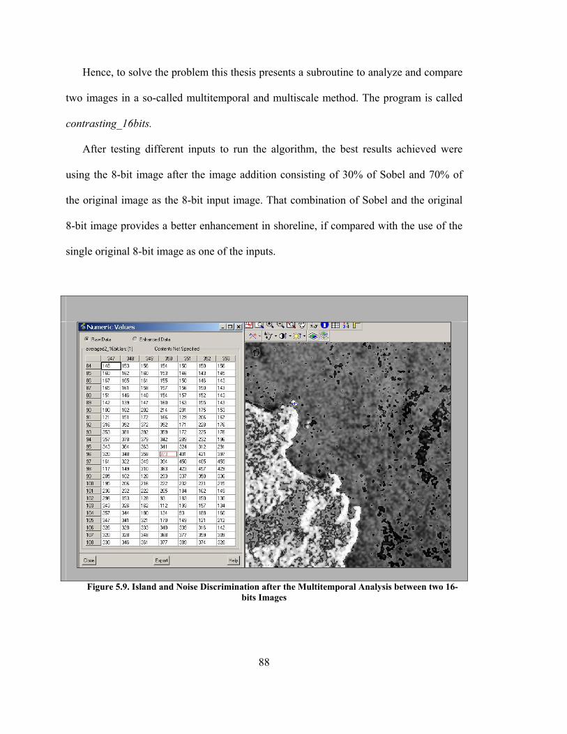
88
Hence, to solve the problem this thesis presents a subroutine to analyze and compare
two images in a so-called multitemporal and multiscale method. The program is called
contrasting_16bits.
After testing different inputs to run the algorithm, the best results achieved were
using the 8-bit image after the image addition consisting of 30% of Sobel and 70% of
the original image as the 8-bit input image. That combination of Sobel and the original
8-bit image provides a better enhancement in shoreline, if compared with the use of the
single original 8-bit image as one of the inputs.
Figure 5.9. Island and Noise Discrimination after the Multitemporal Analysis between two 16-bits Images
89
The operator must analyze the critical areas and chose a threshold in the 8-bit image
and the 16-bit image. The program first reads the enhanced Sobel 8-bit image, and then
if the pixel value is above the threshold, it analyzes the second image. Otherwise, it sets
the pixel to zero (rough land-water segmentation). Then, in the second image, if the
pixel value is above the threshold, the pixel value in the output is set as the pixel value in
the 8-bit image (keeping most of the land radiometric characteristics), otherwise, a mean
window is applied over the center and its neighboring pixels in the 8-bit image
(smoothing the noise over the sea surface).
The effect of comparing an 8-bit Sobel enhanced image and a 16-bit image is shown
in Figure 5.10. This procedure performs a kind of segmentation, setting most of water
pixels to zero while smoothing the pixel corresponding to noise in water and maintaining
the enhancement of most of the pixels corresponding to land. The ideal threshold should
not affect the pixel values corresponding to shadow or wetland areas (practically an
impossible task because the radiometric and geometric characteristics of radar images).
This time, the threshold was chosen according to the mean value for both 8-bit and
16-bit images. It gives a desirable separation between land and water.
After this procedure, opening operation (digital morphology) is applied to the image
to destroy and smooth most of the edges in water (noise), giving acceptable results.
Once the opening operation has been done, the resulting image is contrasted again
with the 8-bit image, but this time the effect of this operation is to enhance most of the
land pixels with respect to the noise pixels over the water. This new subroutine is called
“island enhancement”.

90
Figure 5.10. The Resulting Image after Applying Multi-Image Segmentation
In this case, the output from the opening operation is used together with the original
8-bit image in the new module called island enhancement. This sub-routine enhances the
values over land while keeping the gray-level value of the noise after the opening
operation.
The enhancement of pixels having 255-value is done according to the values of the
pixels in its neighborhood. If the pixel corresponding to land is connected at least with
three pixels with value corresponding to 255, then the center pixel and the complete 3x3

91
surrounded window is set to 255 unless the neighbor pixels correspond to water (pixels
with value equal to zero). The results of this operation were good because it made the
island-noise discrimination better. Also, pixels having zero gray-level values are not
affected by this operation. Consequently there is no offset in the shoreline
The result of this operation is shown in Figure 5.11. Most of the land pixels have
again 255 gray-level values, while the gray-level value in the pixels corresponding to
noise remains smoothed and with lower value if compare with islands.
Figure 5.12 shows also a zoom and numeric values to display the effect of this
operation that increases most of the gray level pixel values of land and islands.
Figure 5.11. The Effect after Enhancing Land Pixels
The pixels in the image after opening operation (left) are enhanced as shown in the right image.

92
Figure 5.12. Numeric Values of Pixels in Land and Noise
However, there is still too much noise present in the sea, which could be
misinterpreted as false islands. In the process of reducing that noise, again the image
after being enhanced is compared with the segmented (binary) image obtained after the
application of common filters.
Using the subroutine called “contrasting bitmap”, if zero-values are found in any of
the input images, the output is set to zero. This operation ensures the reduction of the
noise when it is excessively large in the image. If the noise is not too big, this stage could
be jumped and the direct application of windows to delete noise proceeds.
The effect of this operation is displayed in Figure 5.13. The most important
achievement of this operation is that the noise now has a gray level value different from
the gray-level value of islands in the image.

93
Figure 5.13. The Enhanced Image after the Multitemporal Segmentation Method
After the operations described in this section, the input image is improved and now it
is ready for the application of windows designed to delete the remaining noise over the
sea surface.

94
5.6 A Window-based Algorithm to Eliminate the Noise
After the enhancement of the input image, the next task was to improve a procedure
to remove the noise while keeping the pixel values in land.
Because that noise is local and it could be easily confused with islands, this approach
was achieved using a basic “star–shape” (Figure 5.14) window analyzing the presence of
zero-values in the neighborhood of the center pixel, considering vertical horizontal and
diagonal directions. The size of the window depends of the size of the noise to be
removed. The size of the window is usually large (15x15 and up) to remove large
extensions of noise.
Figure 5.14. The Window used to Remove Noise and to Fill the Gaps
This window is based on the analysis of pixel values in the vertical, horizontal and diagonal directions.

95
As a result of the analysis in eight directions, a great amount of noise has been
removed, but as seen in Figure 5.15, some portion of the coastal zone is deleted too. To
refine the window, now sixteen directions were analyzed. Hence, the noise is removed
just when the analyzed pixel is different to zero (of course water) or 255 (enhanced
islands and most of land pixels).
The window analyzes in the first direction, if zero value is not found the pixel
remains with the same value and the next pixel is analyzed. If zero value is found in the
first direction, it initiates a counter and the second direction is analyzed. If the counter
reaches sixteen, then the central pixel is set to zero, otherwise no changes are made to
the analyzed pixel.
Especially, close to the land, some remaining spots will still remain in the output
image. That noise can be deleted using a small window as shown in Figure 5.16.
Figure 5.15. Application of Basic Star-shaped Window
Figure 5.16. Application of Small 3x3 Window

96
After the noise is deleted, morphological operations (dilation and closing) can be
used to fill the gaps and join the broken segments in the bitmap image as shown in
Figures 5.17 and 5.18.
At this stage, the results are more acceptable in shoreline detection. However, while
testing the results in different areas, the excessive amount of gaps caused by this
operation was detrimental in the final results. Therefore, it was necessary to refine the
window used to delete noise and to find the way to fill most of the undesirable gaps in
land.
Figure 5.17. A 5x5 Dilation Operation Figure 5.18. A 3x3 Closing Operation
5.6.1 An Iterative Method to Delete Noise and to Fill Gaps

97
As described by Zhang (2000), methods for connecting broken linear segments and
eliminating noise are important. Especially in the case of radar images in which the pixel
values depend of land or water roughness, that noise should be eliminated to achieve
continuous feature extraction.
Zhang (2000) describes a method to extract urban rivers. The continuous extraction
of linear objects, such as rivers, roads or boundaries, from digital images can hardly be
achieved using automatic methods. Line extraction algorithms usually break down linear
objects into segments with significant noise.
The same problem is present in shoreline extraction. After processing the image,
there is some noise in water as well as some gaps in land due to shadows in the image or
simply wetlands or lakes. Hence, the application of an algorithm to fill those gaps in
coastline segments and to remove the noise in the sea surface is applied to the image.
Therefore the process of segmentation and connection has to be carried out
iteratively. Noise is removed step by step and coastline segments are also restored step
by step. This procedure is based in windows designed to operate over the image deleting
the noise and filling some holes in land.
The key to achieve this window operation was the enhancement of input image
described early in this chapter. After that enhancement, the reduction of noise in water
and the process to fill the gaps in land are made iteratively until the noise is gone. After
that, the continuous application of the function to fill the gaps could be applied to the
image combined with closing operations if necessary.
The result of this operation will produce a new image without noise and with most of
the gaps closed.

98
The whole process of this window operation is described in Figure 5.19 and the
result of the application of the windows is shown in Figure 5.20.
Figure 5.19. Iterative use of Windows to Delete the Noise and to Fill the Gaps
Because the size of the window is sometimes not enough to close completely the
largest gaps, usually there are some remaining gaps after this processing stage. These
remaining gaps could be undesired, especially if they are still close to the shoreline. To
fill those rectangles, a simple closing window (morphological operation) could be used.
The result of this closing operation is shown in Figure 5.21.
REMOVING NOISE FILLING GAPS
Yes
FILLING GAPS
No
Yes
No
CONTRASTING WITH THE ORIGINAL IMAGE TO RE-OPEN
CLOSED BAYS
Still noise?
Gaps filled?

99
Figure 5.20. The Image after Most of the Gaps are Closed.
Figure 5.21. The Image after Closing Operation using Digital Morphology.
Because filling gaps or closing operation could affect little indented bays, rivers or
deltas, the image is contrasted again with the original image to open those areas with a
pixel value that approximately corresponds to the mean pixel value in water areas
(enclosed bays).
The original image usually has no problem of noise in enclosed bays (less wind) as it
has in the open sea areas. Because some gaps filled in the image correspond to real
lakes, bays or rivers, they are restored again using the original image.
After this procedure, it is possible to segment the image to finally detect the
shoreline without the problem of noise. Also, most of the problems in shoreline
detection are solved with the exception of some little problems because the presence of
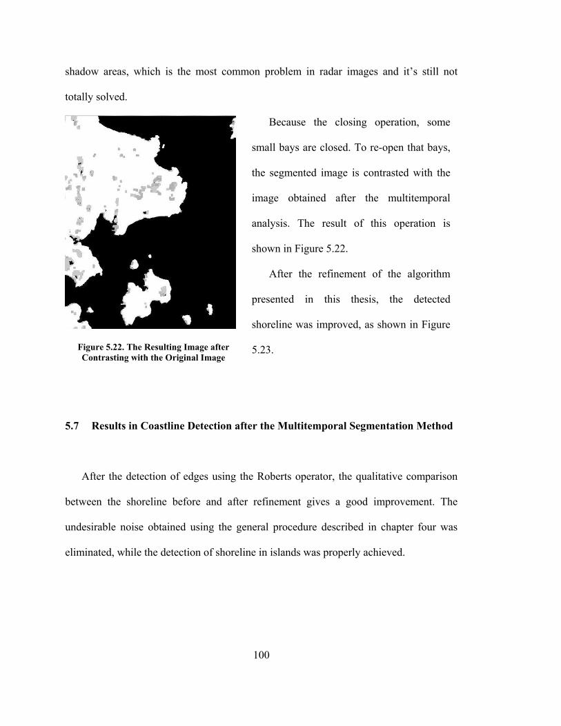
100
shadow areas, which is the most common problem in radar images and it’s still not
totally solved.
Figure 5.22. The Resulting Image after Contrasting with the Original Image
Because the closing operation, some
small bays are closed. To re-open that bays,
the segmented image is contrasted with the
image obtained after the multitemporal
analysis. The result of this operation is
shown in Figure 5.22.
After the refinement of the algorithm
presented in this thesis, the detected
shoreline was improved, as shown in Figure
5.23.
5.7 Results in Coastline Detection after the Multitemporal Segmentation Method
After the detection of edges using the Roberts operator, the qualitative comparison
between the shoreline before and after refinement gives a good improvement. The
undesirable noise obtained using the general procedure described in chapter four was
eliminated, while the detection of shoreline in islands was properly achieved.

101
Figure 5.23. The Detected Coastline after using the M.S.M. Developed in this Research
•
• c
• • • •
102
5.7.1 Testing the Refined Algorithm in Different Areas
Except a little problem caused by the inevitable shadow caused by a steeper hill, the
algorithm seems to work properly in the area tested during the previous section.
However, to ratify the efficiency of the algorithm it is absolutely necessary to test other
areas with different geographic characteristics.
The same procedure described in this chapter was applied to other areas with
different environmental and geographic characteristics. Areas with indented fiords and
bays, mountains causing undesirable shadows and wetlands, which produce low
backscatter in the returning signal, were tested.
After the refinement performed in this chapter, the noise in the sea surface has been
solved, but there are still gaps in the land areas because the radiometric characteristic of
radar images related to geographical relieves.
Also, because this procedure attempts to find a solution for coastline detection, those
gaps present in land are not totally solved but improved using this algorithm.
It is important to mention that this algorithm is based in the land-water enhancement.
Hence, this algorithm is enhancing the shore areas using a technique based in the
destruction off most of the land edges, while preserving the most important: the
coastline.
During the analysis of the other areas, the results were not perfect if compared with
the result achieved in the study area presented before in this chapter. Because their size,
some gaps could not be closed; however they rarely affect the correct delineation of the

103
shoreline. To avoid that, closing operations can be performed if necessary, unless the
area is indented, and it presents high backscatter of the sea surface close to the land.
As shown in Figure 5.24, the results observed in those four different areas are quite
good output to delineate the coastline because the edge corresponding to the shoreline
has been isolated from other edges of the image. The unsolved gaps encountered in
landward directions are just visually negative because they are not affecting the final
shoreline extraction. The coastline has been well defined, without the influence of
undesirable noise that could produce misinterpretation of that required edge. Even in the
top-left image (Area 1), which is the most difficult scenario to detect the shoreline
because the amount of small fiords and the fuzzy shoreline definition in another areas,
however, the coastline is continuous over its extension.
The last step in this method is the extraction and vectorization of the detected
shoreline in the raster image, as described in chapter 7.

104
Area 1
Area 2
Area 3
Area 4
Figure 5.24. Four Different Areas where the Algorithm was Tested

105
5.8 Summary
The Multitemporal Segmentation Method was successfully used to achieve a proper
land-water separation in critical areas subject enormous influence of environmental
conditions such as wind.
The success achieved in land-water segmentation was fundamental for further
delineation of the coastline in the analyzed images.
Even when, other small edges were detected in land areas, those edges do not affect
the delineation of the coastline, because of the enhancement applied to the shore areas.
After the enhancement using the Multitemporal Segmentation Method, the use of
windows to get rid of the noise caused by the strong backscatter in the sea surface,
achieved the main objective stated in this thesis.

106
Chapter 6
RESULTS AND DISCUSSION
6.1 Introduction
Like any scientific measurement, some inherent errors are associated with shoreline
position data. Quantifying shoreline position and change requires a thorough
understanding of coastal processes, mapping fundamentals, and measurement theory.
The challenge for quantifying change is that researchers must not only know the most
modern methodologies, but they also should have a thorough understanding of how
historical shoreline data were captured.
All maps and digital geospatial data are abstractions of reality and, therefore, they
have inherent uncertainties.
In order to apply the detected coastline for GIS purposes, in this chapter the average
error in coastline detection using M.S.M. is analyzed and compared with the average
error obtained if the coastline is detected after the application of common filters and the
reduction of noise using multitemporal analysis described in section 5.3.4, showing the
improvement achieved in coastline detection.
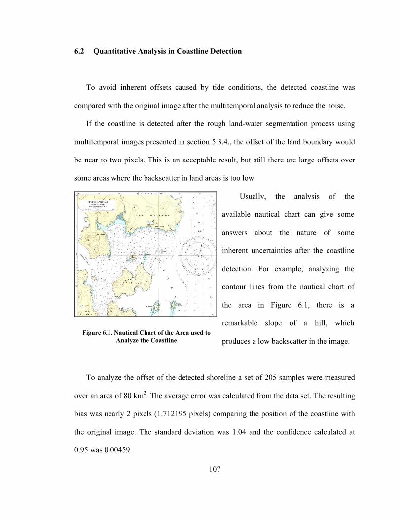
107
6.2 Quantitative Analysis in Coastline Detection
To avoid inherent offsets caused by tide conditions, the detected coastline was
compared with the original image after the multitemporal analysis to reduce the noise.
If the coastline is detected after the rough land-water segmentation process using
multitemporal images presented in section 5.3.4., the offset of the land boundary would
be near to two pixels. This is an acceptable result, but still there are large offsets over
some areas where the backscatter in land areas is too low.
Figure 6.1. Nautical Chart of the Area used to Analyze the Coastline
Usually, the analysis of the
available nautical chart can give some
answers about the nature of some
inherent uncertainties after the coastline
detection. For example, analyzing the
contour lines from the nautical chart of
the area in Figure 6.1, there is a
remarkable slope of a hill, which
produces a low backscatter in the image.
To analyze the offset of the detected shoreline a set of 205 samples were measured
over an area of 80 km2. The average error was calculated from the data set. The resulting
bias was nearly 2 pixels (1.712195 pixels) comparing the position of the coastline with
the original image. The standard deviation was 1.04 and the confidence calculated at
0.95 was 0.00459.

108
There were several outliers caused by the strong sea backscatter close to the
shoreline and the failure of the rough method using common filters to detect the
shoreline. This situation is incremented over sinuous coastline configuration, especially
when rough sea surface is close to the shoreline.
Without considering the outliers, and after the application of dilation procedure
presented in section 5.4 [Lee and Jurkevich, 1990], the same 205 pixels used to calculate
the average error were again analyzed. This time, the bias over that “wind-forced” noisy
image was nearly one pixel offset (1.009), the standard deviation was 0.99 and the
confidence calculated at 0.95 was 0.0043. However, the outliers are still present in the
detected shoreline.
After refining the coastline detection with the algorithm proposed in this thesis, the
same analysis over the 205 pixels was done, minimizing the average error and
consequently giving more precision in the coastline extraction.
The achieved one-pixel offset means a shifting of 12.5 metres in reality. If it is
represented in a nautical chart with a scale of 1:60,000, this offset represents a shifting
of 0.2 mm.
The following table gives the bias in coastline before and after the algorithm
proposed in this thesis. The samples were analyzed every 5 pixels in the coastline. The
average error or bias using the M.S.M. in the images was considerably lower than the
resulting coastline using common filters and the refinement used by Lee and Jurkevich
[1990].

109
Table 6.1. Comparison between the use of Most Common filters and the M.S.M
ANALYZED AREA Average error after using common filters
Average error after the M.S.M. and the iterative use of
windows Area 1 1.073 0.909
Area 2 1.009 0.825
Area 3 0.834 0.775
Area 4 0.790 0.741
Area 5 1.892 0.985
6.3 Qualitative Analysis in Coastline Detection
After the analysis of the images it was possible to identify some critical situations
regarding the configuration of the coast and environmental parameters, which affect the
automatic delineation of the coastline. The most critical topographic features and
environmental processes in the detection of shoreline can be described as follow:
- Shadows areas caused by hills close to the shoreline
The main problem of radar images (shadowing caused by relief) is present here and
it is the most difficult problem to solve in automatic delineation of shoreline when it is
close to the land-water boundary.

110
Figure 6.2. The Effect of Shadow Caused by Step Relieves such as Hills or Trenches Left: The detection of shoreline using the most common procedure. Right: The detection of shoreline using the M.S.M.
After the coastline detection using the M.S.M. this problem is partially solved.
However the operator still must pay attention to this kind of problem.
- Wetlands, which produce low backscatter
Another unsolved problem is the low backscatter coming from flooded areas or
wetland. In fact, the coastline is in the place where water ends. If the wetland is close to
the shoreline, that shoreline will be placed where the land starts. The operator must
analyze quite well the areas with an optical image or analyzing the old map to verify the
presence of beaches, salty and shallow lagoons, deltas etc. Figure 6.3 shows the effect of
coastline delineation considering a flooded area with the connection with a small river.
Figure 6.4 shows the map and photography of the area with problems.

111
Figure 6.3. The Low Backscatter of Flood Areas or Wetland Produces a Misinterpretation of the Shoreline
Left: The detection of shoreline using the most common procedure. Right: The detection of shoreline using the M.S.M.
Figure 6.4. Information used to Visually Analyze the Coastline in Areas with Problems Bottom Left: The area illustrated in the nautical chart. Bottom Right: The same area from the aerial photo.
- Islands close to the main shoreline

112
Due to the spatial resolution of the image, while the enhancement of land-water
boundary is taken effect, the shoreline is displaced seaward in most of the spatial
methods used to delineate the shoreline. This is the case of Erteza [1998] method or Lee
and Jurkevich [1992] method (1 pixel or two). Figure 6.5 shows the improvement made
over areas where islands are too close to land, if using the M.S.M.
Figure 6.5. The Effect of Shoreline Delineation in Cases where the Islands are Close to the Main Shoreline
Left: The detection of shoreline using the most common procedure. Right: The detection of shoreline using the M.S.M.
Using the proposed method to detect the shoreline, the offset is reduced. Hence,
most of the islands close to the land are detected without merging them. Also if the
resolution of the image to be used is better, this problem could be further solved.
- Narrow channels or straits, with indented shape

113
As the same situation of the islands close to the land, narrow channels could be
closed and misinterpreted. With the M.S.M the offset of the shoreline is solved in most
of the cases. Figure 6.6 shows how a narrow channel is correctly delineated. Hence, the
shoreline can be automatically vectorized successfully.
Figure 6.6. The Effect of Shoreline Delineation in Cases of Narrow and Indented Channels Left: The detection of shoreline using the most common procedure. Right: The detection of shoreline using the M.S.M.
- False edges on the sea surface caused by wind
Noise over the sea surface can be presented in ways such as small dots, large spots
with regular or irregular shape, etc. However, one of the most complicated types of noise
is the one that produces a well-defined edge in water surface caused by local stream
wind. If one of the images used in the multitemporal analysis has too much noise, that
noise is just smoothed a little bit and the resulting image will still have this “false edge”.
After the refinement using the M.S.M. this problem is solved.

114
Figure 6.7. The Effect of False Edges in Water Areas and how the Algorithm can Discriminate False from Real Edges
Left: The detection of shoreline using the most common procedure. Right: The detection of shoreline using the M.S.M.
This effect can be observed in Figure 6.7. If using traditional filters, there is still an
excessive noise in the middle of the canal and an undesirable edge caused by the contrast
of rough surface (wind) and calm water. Hence, the main shoreline was delineated with
a large offset. However, applying the M.S.M., the gray-level value of that noise is lower
than the gray-level value of land in the canal.
After the refinement, and because this thesis uses the radiometric characteristic of
images in 8-bits and 16-bits, this problem was solved.
The principal problems in the detection of shoreline after the application of common
filters are the use of relatively large windows (5x5 smoothing and closing principally).

115
After the segmentation and 5x5 binary closing coarse land-water segmentation was
achieved. That segmented image is further used just to eliminate most of the wind-
forced noise in the M.S.M presented in chapter 5.
Besides the better results in the bias obtained in shoreline extraction, most of the
shoreline delineation over those critical areas was solved with the refined algorithm,
solving a great amount of the outliers detected during the first approach.
Also, it is obvious but necessary to mention that the land-water enhancement and
discrimination produces the elimination of all the image features except the shoreline.
Hence, after histogram scaling, most of the land features are gone and land analysis
could not be performed.
6.4 Summary
In all the areas tested, the problem of excessive noise over the sea surface was solved
using the Multitemporal Segmentation Method. Also the offset of the detected shoreline
was improved.
Because the algorithm fails in few cases mentioned above and some coastlines are
misinterpreted causing some offset in few areas, the analysis of the operator in this semi-
automatic algorithm is very important to correct those errors during the vectorization
procedure.

116
Chapter 7
APPLICATION OF THE DETECTED COASTLINE FOR GIS PURPOSES
7.1 Introduction
The detected coastline now can be extracted using a contour following algorithm. In
this project, the shoreline was exported to a GIS environment and vectorized using
CARIS SAMI.
However, the vectorized coastline must be referenced to a tidal level. This concept is
just outlined in this chapter, but must be taken in account when using the shoreline to
update nautical charts.
7.2 Vectorization of the Coastline using CARIS SAMI
CARIS SAMI is an interactive program designed to create and edit digital maps. A
digital map is a computerized version of a traditional map. CARIS (Computer Aided
Resource Information System) stores a digital map as a CARIS file.
An efficient method of converting large volumes of paper maps into a digital vector
format is to scan the map sheets and convert the resulting raster data to vector

117
Raster data consists of rows and columns of pixels (rectangular cells with a single
grey level value between 0 and 255 with 0 being black and 255 white). CARIS SAMI
requires a single bit file where the pixel value is either 0 or 1.
Vector data consists of lines, points and text. The vector format is used in most
Geographic Information Systems (GIS) and computer aided drafting (CAD) systems.
CARIS SAMI has integrated the two formats to efficiently handle the conversion of
large volumes of data.
The vectorization of the coastline information is fundamental to insert the extracted
coastline in a vectorized environment such as the Digital Nautical Chart (DNC).
One of the purposes of extracting the coastline from a satellite image is the updating
of this important feature in existing nautical charts. Hence, the vectorization of the
coastline using CARIS SAMI gives an important solution to update the coastline
information in the same software used to compile the DNC.
7.2.1 Procedure to Export the Image as CARIS SAMI File
CARIS SAMI is a Microsoft Windows based application. The software is user-
friendly and it has a wide range of options and functions to work with raster data.
After the detection of the shoreline and the other few remaining edges, there are two
alternatives to do with the data:

118
The first one consists in transforming the data to DXF vector format. A DXF file is a
drawing interchange format file developed by Autodesk. This is a file type used for
facilitating data exchange between CAD systems.
Just as CARIS has visibility parameters, DXF has layers to allow users to define
what is displayed on screen. Because AutoCAD is primarily a drafting tool and CARIS
is meant for information management, there are differences in the approach to separating
data. AutoCAD uses a similar approach to clear acetates, overlaid one on top of the
other. CARIS can group data in a similar manner (using themes) but, because it is a GIS,
it also has the capability to group features by other means, such as geographic data type
(contours, coastlines, etc) [CARIS GIS manual].
The second alternative is exporting the data as TIFF (GeoTIFF) file, and using that
raster file to vectorize the data in SAMI. "GeoTIFF" refers to TIFF files, which have
geographic (or cartographic) data embedded as tags within the TIFF file. The geographic
data can then be used to position the image in the correct location and geometry on the
screen of a geographic information display.
I used the second option because instead of having all the edges transformed to
vectors, the aim is to vectorize just the usable edge, which is the shoreline. Therefore,
once in SAMI environment, the coastline is selected and the contour following algorithm
is applied as follow.
After the shoreline detection using the algorithm presented in chapters 5, the
resulting raster image is transformed into TIFF format. However, it is necessary to
manipulate the pixel values using image processing software such as Photoshop
applying contrast and converting the image into bitmap image (0 and 1).
119
After that, using the tools mode of CARIS SAMI, the image is exported into *.DES
file, which is the standard file format for CARIS. Once converted to *.DES, it is possible
to use CARIS SAMI to open the raster file and to start using the line following or
contour following function in case of island or linear shoreline respectively.
Thinning operation in CARIS SAMI is not necessary because the edges detected are
1-pixel wide after the application of Roberts algorithm.
The procedure is very easy to implement and the operator should concentrate just in
the vectorization of the required edges in the image.
After the vectorization of each completed line, it is important to assign the
corresponding user number to the feature to be vectorized. In this case, the feature code
used for coastline of the coastline was entered as CLSL when required.
Since the coastline was well defined after the application of the algorithm described
in this thesis, the vectorization using the contour following algorithm was done very fast
and straightforward. The generated coastlines after the vectorization are displayed in
Figures 7.1 to 7.5.
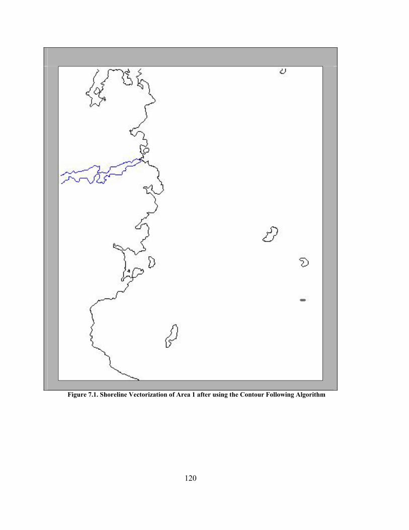
120
Figure 7.1. Shoreline Vectorization of Area 1 after using the Contour Following Algorithm

121
Figure 7.2 Shoreline Vectorization of Area 2 after using the Contour Following Algorithm

122
Figure 7.3. Shoreline Vectorization of Area 3 after using the Contour Following Algorithm
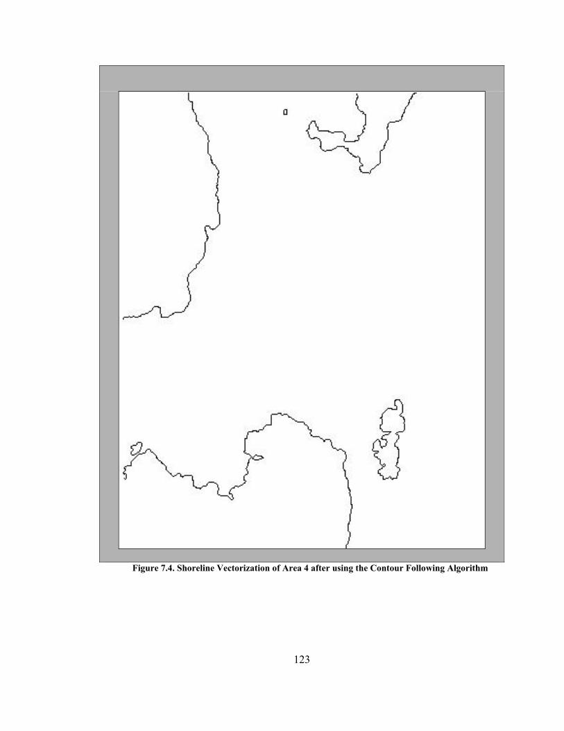
123
Figure 7.4. Shoreline Vectorization of Area 4 after using the Contour Following Algorithm

124
Figure 7.5. Shoreline Vectorization of Area 5 after using the Contour Following Algorithm

125
7.3 The Needs to Adjust the Shoreline with a Tidal Model
For nautical cartography, the desired product is to develop a method for extracting a
Mean Low Low Water (MLLW) vector estimate from imagery. By definition [NOAA,
2004], MLLW is the horizontal vector shoreline determined at an elevation, which is
average of the lower low water height of each tidal day observed over the National Tidal
Datum Epoch (NTDE).
The distance between MLLW and in situ waterline is dependent on the tidal stage
and the daily tidal variability. At high tide, the distance is small (large) for steep
(shallow) shore slopes. Capturing an image near low tide usually reduces this error.
However, low tide elevations are seasonal and can be quite variable. Also, perturbations
from tidal models occur regularly due to environmental conditions [Yeremy et al.,
2001].
For a project like shoreline mapping the logistics of acquiring satellite images at the
local low tide could also be very difficult. Instead, if more accurate shorelines are
required, a waterline estimate can be improved to an MLLW estimate, provided the
appropriate information is available. In particular, the shore slope and a tidal model,
which is geo-referenced (with accurate elevation information), are required. If possible,
local tidal elevations at the acquisition time would also improve the estimate and remove
errors caused by temporal variability [Yeremy et al., 2001].
The requirements to achieve a shoreline extraction referred to the required datum are
summarized as follow [Yeremy et al., 2001]:

126
- Image data.
- Ground truth (extracted waterline could be compared with in-situ measurement).
- Contrast enhancement methods for accentuating the land-water edge in the imagery
(achieved in this thesis).
- A procedure developed for extracting shorelines from this enhanced image data
(achieved in this thesis).
- A method to extract shore slope information.
- Shore slope data potentially can improve a shoreline estimate to MLLW estimate.
- Tidal models referenced to chart datum must be included.
- The addition of in situ tidal elevation data at the image time would also improve the
results.
As shown in Figure 7.6, a simple geometric model can be applied to reference the
extracted shoreline to the desired datum (in this case, the MLLW).
If a shore slope estimate can be determined, then with a sufficient tidal knowledge
the elevation difference (z) between the elevation of the MLLW and in-situ waterlines
provides a distance, which can be projected onto the shoreline.
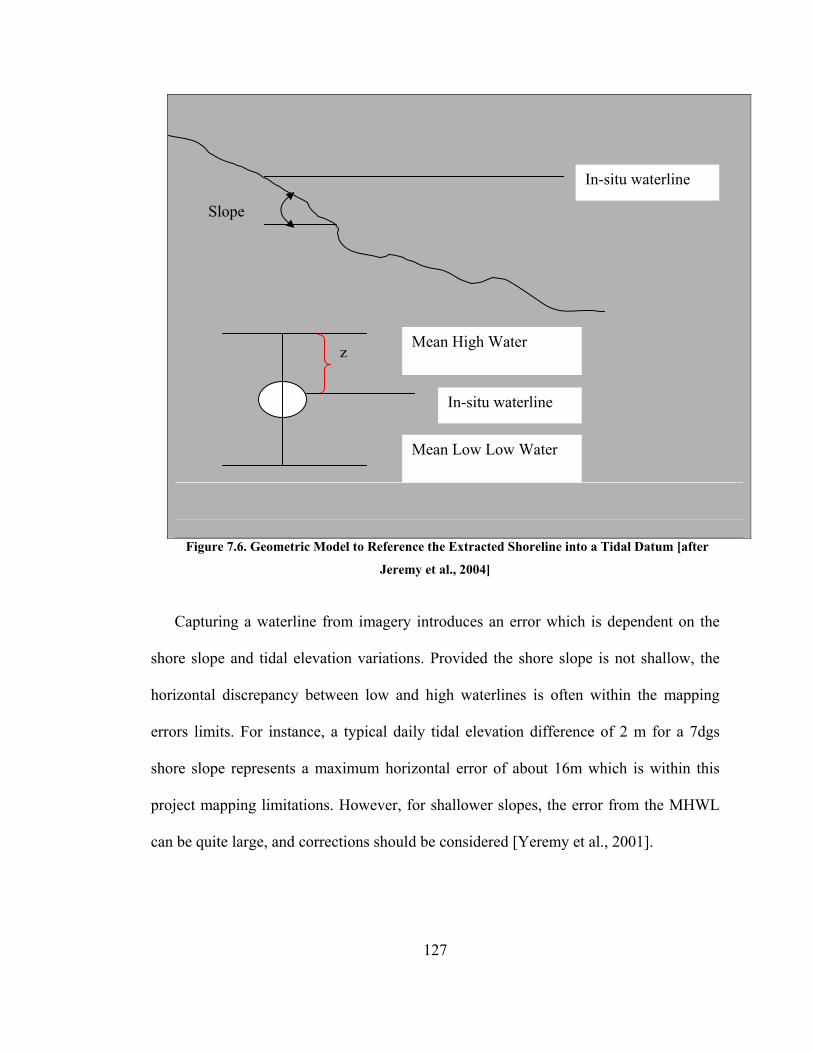
127
Figure 7.6. Geometric Model to Reference the Extracted Shoreline into a Tidal Datum [after
Jeremy et al., 2004]
Capturing a waterline from imagery introduces an error which is dependent on the
shore slope and tidal elevation variations. Provided the shore slope is not shallow, the
horizontal discrepancy between low and high waterlines is often within the mapping
errors limits. For instance, a typical daily tidal elevation difference of 2 m for a 7dgs
shore slope represents a maximum horizontal error of about 16m which is within this
project mapping limitations. However, for shallower slopes, the error from the MHWL
can be quite large, and corrections should be considered [Yeremy et al., 2001].
In-situ waterline
z Mean High Water
In-situ waterline
Mean Low Low Water
Slope

128
In this project, the study area presents high topographic variations. Also the slope of
the beach is very step. After the application of a tidal model, this situstion should
provide small offset between the in-situ waterline and the desired product.
7.4 Summary
In order to use the detected shoreline in a GIS environment, some requirements are
necessary. First, the appropriate extraction of the detected shoreline must be achieved.
Once the shoreline is vectorized, the application of a tidal model is highly necessary
to connect the shoreline to a reference system.

129
Chapter 8
CONCLUSIONS AND RECOMMENDATIONS
8.1 Conclusions
Previous research had been done in shoreline detection. Certainly, the detection of
those important features depends on the quality of the image together with the
environmental parameters at the time of the data acquisition.
Most of the previous works in shoreline extraction using SAR images use
complicated algorithms based in a series of mathematical and statistical procedures to
detect the shoreline, obtaining very good results. However, the studied previous works
do not show results over areas with high environmental conditions such as the area
analyzed in this research.
8.1.1 Regarding the Algorithm
After analyzing the most common procedures used to detect the shoreline, the
general approach to detect the coastline is based on:
- Obtaining a rough separation between the land and water, and

130
- Refining the rough land-water boundaries by edge detection and edge tracing
algorithms to extract the accurate shoreline position.
This thesis has followed these two principal stages. The rough land-water separation
has been achieved using the most common filters after applying the multitemporal
analysis to reduce the noise caused by the strong backscatter over the sea surface.
The second stage was achieved using the Multitemporal Segmentation Method
proposed in this thesis, with excellent results and solving the most common problem in
SAR images: noise on the sea surface. After the successfully shoreline detection, the
edge was extracted using CARIS SAMI.
The M.S.M. is a simple method based in the enhancement of the input image using a
series of operations between two images acquired at different dates.
The traditional method described in chapter 4 corresponds to a coarse procedure to
detect the coastline. Using this coarse method, in section 5.3.4, after the application of
multitemporal analysis to reduce the noise, the shoreline has been roughly detected and
there are still some problems to solve.
However, the segmented image resulting from this rough method is still useful in the
proposed Multitemporal Segmentation Method. So, the rough and the refined shoreline
detection methods are connected and form one single methodology.
The use of windows after the M.S.M., were fundamental to achieve good results.
After the enhancement of the input image, noise and land pixels have their own pattern
in pixel value and distribution. Therefore, a local window that analyzes the pixel having
values different to zero and 255 and their respective neighborhood is used to delete the
noise with very good results.

131
To, fill the gaps in land, the same concept is applied, but in reverse way: detecting
pixel-value equal to zero and analyzing their neighboring pixels.
The process of filling undesirable gaps in land is a little more complex and it still
requires more improvement. The problem comes when the area is indented and contains
small bays and narrow canals. Some gaps cannot be closed and sometimes is necessary
to perform morphological operations (closing) to fill gaps close to the shoreline.
8.1.2 Regarding the Data Used
Regarding the data used for feature extraction, amplitude images are the most used.
Today the use of polarimetric images gives a very good approach to detect the coastline
and it is becoming widely used.
The algorithm applied to the data used in this research can be applied to better
dataset, such as polarimetric images or better images in resolution. The spatial resolution
of radar images is becoming better and consequently, the applications of using those
images for cartography are more and more widely used.
8.1.3 Identification of Main Concepts the Proposed Method
Certainly, the application of the proposed method to detect the shoreline would not
be successful without some very important concepts.

132
The use of multitemporal images was essential to solve the problem regarding the
roughness in the sea surface. Statistical correlation or averaging two images has been
used to reduce the noise on water while keeping the high pixel value in land, with very
similar results. If the available images are more than two, the correlation analysis or
PCA gives better result. However the more images are available, the more expensive is
the cartographic production.
Doing the multitemporal analysis, most of the original noise has been smoothed.
After the noise reduction the sequential application of spatial filters, morphological
operations and edge detection filters were applied to the image to roughly detect the
shoreline. However, the remaining noise in the sea surface still caused some problems in
the shoreline delineation and island detection. That noise usually was misinterpreted as
islands producing undesirable detection of false edges.
The stated question was: how to get rid of that noise without deleting islands or low-
pixels values features in land areas? Instead of using complicated algorithms to solve
that problem and with the fact that usually the pixel-value of that undesirable noise is
higher than some of the pixel values in land (shadows, wetland, etc), this research was
focused in the use of a simple and straightforward procedure based in the inherent
properties of the image and the use of local windows to delete that noise without
affecting the land pixels.
The time saved using this procedure if compared with the traditional methods of
digitization of the contours constitutes a great improvement in the cartographic
production and updates of existing maps.

133
Even when automatic coastline detection methods give very good results to save
time during the tedious process of digitalization, the analysis of the operator in the final
revision is very important to avoid wrong interpretation of critical areas.
8.2 Recommendations
A simple and effective algorithm to detect the coastline has been described in this
thesis. After the coastline detection, the extraction of that coastline has been achieved
using CARIS SAMI, in a fast and reliable procedure to vectorize the shoreline
information.
The shoreline that has been extracted should be related to the tide information at the
time of image acquisition. So, this shoreline information corresponds to the in-situ
waterline.
For nautical cartography requirements, the desired product is the Mean Low Low
Water (MLLW) vector estimate from imagery.
To achieve that desired result, one solution is trying to acquire the image in low
during low tide condition. The other way is by estimating the shore slope.
8.3 Further work and development

134
Once integrating tidal information together with the shoreline, an important, but
often overlooked issue is: how is the data going to be used? What will be the scale of the
map to be updated and the different uses (military, navigational, tourism, environmental
studies, etc). Is the area a commercial navigational route? What risks involve the
existence of uncertainties in the coastline delineation?
In this case the shoreline can be used to improve existing shorelines or to have
shoreline information from unmapped areas. Because of the resolution of the image used
(12.5 m) the detected shoreline could be used in charts with a scale of 1:70.000 or less
(intermediate to small scale nautical charts).
The development of a semiautomatic methodology to detect the shoreline using
single ERS-1 SAR images gives a powerful to extract coastline from remote areas for
mapping purposes. This application of coastline detection can be extended also to the
Antarctic Continent. SHOA is producing nautical cartography over the areas in the
Antarctic. Some portions of the Antarctic Coast have never been accurately mapped, and
other portions have experimented dramatic changes in position and shapes since they
were mapped. Information about geographic position, orientation, and geometric shape
of the Antarctic coastline is essential for geographic exploration, and nautical and aerial
navigation.
Constructing an accurate coastline map is an important step toward establishing a
baseline for the Nautical Chart and also for future change detection studies in order to
understand the response of remote and southern areas such as the Antarctic Ice sheet to
climate change.

135
The different subroutines were designed to work with images limited by size 800 x
650 pixels. Further work must be done to work with large amount of data with lower
spatial resolution.

136
REFERENCES
Alegria L. (2003). “The Military Geographic Institute of Chile as a Tool For National Development.” Ordnance Survey. Paper presented in Cambridge Conference. [On-line] 03 February 2004. http://www.cambridgeconference2003.com/camconf/papers/3-5.pdf
Alvial A. and D. Recule (1999) “Foundation Chile and the integrated management of the
coastal zone.” Ocean & Coastal Management, Vol.42, Num. 5, pp. 143-154. Asociacion de Productores de Salmon y Trucha de Chile APSTC (2000). “La
salmonicultura en Chile.” Unpublished pamphlet. Santiago, Chile: APSTC (AG). [On-line] 03 February 2004. http://www.globefish.org/publications/commodityupdate/200201/200201.htm
Barret G., M. Caniggia and L. Read (2002). “There are more vets than doctors in Chiloe: Social and Community impact of the globalization of Aquaculture in Chile.” World Development, Vol. 30, Num.11, pp. 1951-1955.
Caris GIS V.4.4a.4.0 (2004) CARIS Universal System Limited. Fredericton, N.B.,
Canada. Caris SAMI Tutorial. Caris GIS V.4.4a.4.0 (2004) CARIS Universal System Limited. Fredericton, N.B.,
Canada. Caris SAMI User’s Guide. Chen, L.C. and C.C. Shyu (1998). “Automated Extraction of Shorelines from Optical
and SAR Image.” [On-line] 10 March 2004. http://www.gisdevelopment.net/aars/acrs/1998/ps3/ps3013.shtml
Erteza, I (1998) “An Automatic Coastline Detector for Use with SAR Images”. Signal
Processing and Research Department. Sandia National Laboratories [On-Line] 13 September 2003. http://www.osti.gov/dublincore/gpo/servlets/purl/1322-XIfWqu/webviewable/1322.pdf
European Space Agency (2004). Earth Observation. Radar Course [On line] 12 August
2004. http://earth.esa.int/applications/data_util/SARDOCS/spaceborne/Radar_Courses/Radar_Course_I/image_geometry.htm
Henderson, F.M., and A.J. Lewis (1998). Vol. II of Principles and Applications of
Imaging Radar. Third ed., Wiley & Sons, USA. Hydrographic and Oceanographic Service of the Chilean Navy (S.H.O.A.). [On-line] 04
February 2004. http://www.shoa.cl

137
James, M. (1987). Pattern Recognition. BSP Professional Books, Oxford, London,
Edinburgh, Boston, Melbourne, 144p. Lee, J-S and I. Jurkevich (1990) “Coastline Detection and Tracing in SAR Images.”
IEEE Transactions of Geoscience and Remote Sensing, Vol.28, Num.4, pp. 662-668.
Liu, H. and C. Jezek (2004). “A Complete High-Resolution Coastline of Antarctica from
Orthorectified Radarsat SAR Imagery.” Photogrammetric Engineering and remote Sensing, Vol. 70, Num. 5, pp. 605-616.
Manfredini J.S. (n.d.). “Aportes del Servicio Aerofotogrametrico en la Produccion y
actualizacion de Cartografia.” [On-line] 12 March 2004. http://www.saf.cl/ Martin, A. and S. Tosunoglu (n.d.) “Image Processing Techniques for Machine Vision.”
Florida International University. Department of Mechanical Engineering [On-line] 20 May 2004.
http://www.eng.fiu.edu/me/robotics/elib/am_st_fiu_ppr_2000.pdf Mason D. and J. Davenport (1996). “Accurate and Efficient Determination of the
Shoreline in ERS-1 SAR Images.” IEEE Transactions on Geoscience and Remote Sensing, Vol.34, Num.5, pp. 1243-1253.
Military Geographic Institute Of Chile (IGM) (2003). “Report On Cartography In The
Republic Of Chile 1999 – 2003”. [On-line] 10 February 2004. http://www.igm.cl/Images/ICAreport.PDF
National Oceanic and Atmospheric Administration (2004). [On-Line] 20 July 2004. http://co-ops.nos.noaa.gov/mapfinder/mllw.html Noble, J.A., (1996). “The effect of Morphological Filters on Texture Boundary
localization.” IEEE Transactions of Pattern Analysis and Machine Intelligence. Vol 18, Num.5, pp. 554-561.
Parker, J.R. (1997). Algorithms for Image Processing and Computer Vision. First ed.,
Wiley & Sons, USA. RADARSAT International (2004). [Online] 04 April 2004. www.rsi.ca Richards, J.A., and X. Jia (1999). Remote Sensing Digital Image Analysis, an
Introduction. Third ed., Springer, Berlin.

138
Schultze, M and Q. Wu (1995) “Noise Reduction in Synthetic Aperture Radar Imagery using a Morphology-Based Nonlinear Filter.” Proceedings of DICTA95. Digital Image Computing: Techniques and Applications, pp 661-666. [On-Line] September 13th 2003. http://www.markschulze.net/docs/pdf/dicta95.pdf
Schwäbisch, M., S. Lehner and W. Norbert, 1998. “Coastline Extraction Using ERS
SAR Interferometry”. [On-Line] 14 September 2004. http://earth.esa.int/symposia/papers/schwaebisc
Serra, J., and L. Vincent (1992). “An overview of morphological filtering.” IEEE
Transaction on Circuits, Systems and Signal Processing. Vol 11, pp. 357-393. Sternberg, S.R., and J. Serra, (1986). “Special Section on Mathematical Morphology”.
Computer Vision, Graphics and Image Processing. Vol 3. pp. 279. The Alaska Satellite Facility (2004). Radar Distortions [On-Line] 20 July 2004.
www.asf.alaska.edu Touzi, A., A. Lopes and P. Bousquet (1988). “A Statistical and Geometrical Edge
Detector for SAR Images”. IEEE Transactions on Geoscience and Remote Sensing, Vol.26, pp. 764-773.
Yeremi M., A. Beaudoin, J. Beaudoin and G. Walter ([2004). “Global Shoreline
Mapping from an Airborne Polarimetric SAR: Assessment for RADARSAT 2 polarimetric modes.” Defence R&D Canada. Technical Report. DREO TR 2001-056.
Yu, Y. and S.T. Acton, (2004). “Automated Delineation of Coastline from Polarimetric SAR Imagery”. Int. Journal of Remote Sensing, Vol. 25 Num.17, pp. 3423-3438. Wolf, P. and B. Dewitt (2000). Elements of Photogrammetry with applications in GIS.
Third ed., Mc. Graw Hill, USA. Xiao, J., J. Li and A. Moody (2002). “A Detail-Preserving and Flexible Adaptive Filter
for Speckle Suppression in SAR Imagery”. International Journal of Remote Sensing, Vol. 24, Num. 12, pp. 2451-2455.
Zelek J. (1990). “Computer-aided linear Planimetric Feature Extraction” IEEE
transactions on Geoscience and Remote Sensing. Vol.28, Num.4, pp. 567-572. Zhang, Y. (2000). “A method for Continuous Extraction of Multispectraly Classified
Urban Rivers”. Photogrammetric Engineeering & Remote Sensing. Vol.66, Num.8, August 2000, pp. 991-999.

139
Appendix I
STEPS TO PERFORM COASTLINE EXTRACTION USING THE
MULTITEMPORAL SEGMENTATION METHOD
The proposed algorithm is based in sequential operations using ENVI 4.0 software
and a series of developed subroutines stored in attached CD. The procedure is
straightforward and easy to implement in any computer having ENVI and Microsoft
Visual C++ software.
To run all the programs in the CD, the input images must be 800x650 pixel and *.lan
files. The following outline is writing here for easy use of this method:
I. Rough Noise Reduction and Land-water Segmentation
1. Preprocessing of the entire image using speckle reduction (3x3 lee filter
recommended).
2. Subseting the image according to the area analyzed. The new image must be 800 x
650 pixels and exported as *.lan file (image1.lan).
3. Repeat steps 1 and 2 with a second image corresponding to the same area.
4. Image-Image registration between image1 and image2 (image2.lan).
5. Histogram scaling in image1 and image2 from 16 bits to 8 bits.
6. Smoothing and enhancement of edges by 3x3 median filter using ENVI.

140
7. Multitemporal analysis of two scaled 8-bit images (image 1 & 2) using the
workspace: D:\chapter5\8bits_imgavg\8bits_imgavg.dsw
This program is designed to work with two 8-bit images
8. Sobel edge detection using ENVI
9. Edges enhancement, adding back the detected edges over the image.
D:\chapter5\Percent\Percent.dsw
This program is designed to work with Sobel and the image after step 7.
10. 5x5 Gaussian filter and 3x3 gray level closing using ENVI.
11. Binary segmentation and 5x5 binary closing using ENVI.
II. Refinement, Land-noise Discrimination and Windows Operations to Delete
Noise
II. a) Input enhancement
12. Multitemporal analysis using the two original 16 bits images using the workspace:
D:\chapter6\16bits_img_avg\percent_16bit.dsw
This program is designed to work with two 16-bit images.
13. Multi-scale image segmentation between the image after step 9 and the image after
step 12 using the workspace:
D:\chapter6\enhancing input\contrasting_16bit\contrasting16bit.dsw
Note: before doing this operation must ensure that the edges-enhanced image is 8-bit.
14. Perform 5x5 gray-level opening using ENVI.

141
15. Island-noise discrimination using the image after step 7 and the image after step 14
using the workspace:
D:\chapter6\enhancing input\island_enhancement\ island_enhancement.dsw
16. Get rid of the noise contrasting the image after step 15 with the land-water
segmentation image after step 11.
D:\chapter6\enhancing input\contrasting_bitmap\ contrasting_bitmap.dsw
II. b) Use Of Iterative Windows to Locally Delete the Remaining Noise in Water
and to Fill Most of the Gaps in Land
17. Deleting noise in the sea surface in the single image after step 16 using the
workspace:
D:\chapter6\deleting noise\removing_noise\removingnoise.dsw
18. Filling the gaps present in land areas the single image after step 17 using the
workspace:
D:\chapter6\deleting noise\filling_gaps\filling_gaps.dsw
19. Iteratively repeat steps 17 and 18 using the previous image as input. Once there is no
more noise in the image, repeat step 18 until no more gaps are refilled.
20. Opening the closed bays in the image after step 19 using the workspace:
D:\chapter6\deleting noise\opening_bays\opening_bays.dsw
21. Roberts edge detection using ENVI.
22. Binary segmentation of the detected edges using the workspace:
D:\chapter6\segmentation\segmentation.dsw

142
23. The resulting segmented edges must be saved as geo-tiff for further vectorization
using CARIS SAMI.

143
Appendix II
THE ERS - SAR PRECISION IMAGE PRODUCT
The SAR Precision Image product is generated on CCT, exabyte or CD in CEOS
format and contains image data (16 bits, amplitude) related to a full scene (100 Km x
100 Km) and all the required annotations. This product can be provided also on
photographic print.
The ERS-x.SAR.PRI product will be generated with image compensation for
antenna elevation gain pattern and range spreading loss and will be addressed to a large
spectrum of users.
The ERS-x.SAR.PRI product is characterized by a set of parameters listed here;
moreover, in order to check the spacecraft parameters during data generation and to test
the quality of the data, a set of flags and parameters are computed and attached in
product annotations. The convention for QA flags setting is that 0 value indicates
nominal condition (no change in parameter or I-PAF QA thresholds not crossed).
The ERS1/2.SAR.PRI product is characterized by:

144
1. Azimuth output = 8200 pixels
2. Range output = 8000 pixels
3. Data representation = integer (Amplitude)
4. Bits per sample = 16
5. Calibration = internal plus image compensation
6. Output medium = CCT, EXABYTE, CD-ROM, photographic print
7. Output format = CEOS
8. Image coordinate system = ground range / zero Doppler
9. Range pixel spacing = 12.5 m
10. Azimuth pixel spacing = 12.5 m
11. Total processed azimuth bandwidth = 60 Hz
12. Number of temporal look = 3
13. Range spectral weighting function = Hamming window (coeff. 0.75)
14. Azimuth spectral weighting function = Hamming window (coeff. 0.75) centred
on estimated Doppler centroid frequency
The ERS1/2.SAR.PRI product contains in the annotations the following flags and
parameters:

145
1. UTC time of the first line
2. The most precise orbit information available
3. Longitudes of the scene centre and four corners
4. Latitudes of the scene centre and four corners
5. PRF code change flag (0 or 1) 1
6. SWST code change flag (0 or 1)
7. Calibration system and receiver gain change flag (0 or 1)
8. Chirp replica quality flag (0 or 1)
9. Input data statistic flag (0 or 1)
10. OGRC/OBRC flag (flag = 0 for OGRC)
11. Number of PRF code changes
12. Number of SWST code changes
13. Number of calibration system and receiver gain changes
14. Number of missing lines
15. Number of duplicated lines
16. 3-db pulse width of replica ACF
17. PSLR of replica ACF
18. ISLR of replica ACF
19. Estimated mean of I input data
20. Estimated mean of Q input data
21. Estimated standard deviation of I input data
22. Estimated standard deviation of Q input data
23. I-Q channels gain imbalance

146
24. I-Q channels phase imbalance
25. PRF code
26. SWST code
27. Calibration system gain
28. Receiver gain
29. Internal calibration data time tag (UTC)
30. Number of valid calibration pulses
31. Number of valid noise pulses
32. Number of valid replica pulses
33. First sample in replica
34. Calibration pulse power
35. First valid replica pulse power
36. Noise signal power density
37. Range compression normalization factor
38. Doppler centroid confidence measure flag (0 or 1)
39. Doppler centroid value flag (0 or 1)
40. Doppler ambiguity confidence measure flag (0 or 1)
41. Output data mean flag (0 or 1)
42. Overall QA summary index (value 0-9)
43. Doppler Centroid confidence measure (processor specification)
44. Doppler Ambiguity confidence measure (processor specification)
45. Estimated Doppler centroid coefficients
46. Estimated Doppler FM rate coefficients

147
47. Estimated Doppler ambiguity number
48. Zero Doppler range time of first range pixel
49. Zero Doppler range time of centre range pixel
50. Zero Doppler range time of last range pixel
51. Zero Doppler azimuth time of first azimuth pixel
52. Zero Doppler azimuth time of centre azimuth pixel
53. Zero Doppler azimuth time of last azimuth pixel
54. Incidence angle at first range pixel
55. Incidence angle at centre range pixel
56. Incidence angle at last range pixel
57. Processor net multiplicative scaling factors
58. Normalization reference range Ro Km (if available)
59. Antenna elevation gain pattern (if available)
60. Absolute calibration constant K (if available)
61. Upper bound K (+3 Std dev) (if available)
62. Lower bound K (-3 Std dev) (if available)
63. Processor Noise Scaling Factor (if available)
64. Date in which K generated (if available)
65. K version number X.Y (if available)
Product Quality Requirements
The ERS1/2.SAR.PRI product satisfies the following quality performances:

148
1. Ground range resolution of IRF < 30 m
2. Azimuth resolution of IRF < 30 m
3. ISLR of IRF < - 8 dB
4. PSLR of IRF < - 18 dB
5. Point target range geometric misregistration 60 m
6. Point target azimuth geometric misregistration 60 m
7. Processor point target linearity > 0.95 over the linear dynamic range
8. Processor point target linear dynamic range = 30 dB
9. Processor gain = fixed at all times

149
VITA Candidate’s full name: John Neville Fleming Baeza Place and date of birth: Valparaíso, Chile August, 08, 1971 Permanent address: Errázuriz 254, Playa Ancha Valparaíso, Chile Schools attended: Liceo Eduardo de la Barra,
Valparaíso, Chile 1985-1988 Naval Academy “Arturo Prat”
Chilean Navy Bachelor in Naval and Maritime Sciences 1989-1992
Universities attended: Naval Polytechnic Academy, Chilean Navy
- Bachelor in Naval and Maritime Sciences with major in Hydrography and Oceanography
1996-1998 - Hydrographic Engineering Course
Certified with Category “A” from the International Hydrographic Organization 1997-1998
University of New Brunswick, Fredericton, N.B., Canada. Department of Geodesy and Geomatics Engineering Master of Science in Engineering Candidate 2002-2004
PUBLICATIONS Fleming, J., 2nd Lieutenant, Chilean Navy (1998). “Aplicación de un Modelo de Dispersión para Accidentes de Contaminación a lo largo de la Costa de Chile”. (“Application of a Dispersion Model for Contamination Hazards along the Chilean Coast”) B.Sc. thesis, Naval Polytechnic Academy, Chilean Navy.