1

FRP Emissions

Johannes W. KaiserEuropean Centre for Medium‐range Weather Forecasts, King’s College London, Max‐Planck‐Institute for Chemistry

Thanks to Niels Andela, Angelika Heil, Ronan Paugam, Martin G. Schultz, Guido R. van der Werf, Martin J. Wooster and Samuel Remy!

GOFC‐Gold Fire ITWageningen, April 2013

2

burnt biomass

Bottom-Up Estimation of Fire Emissions

Ei = FRE x CF x EFi (Wooster et al. 2003/5)

Ei = BA x AFL x CC x EFi (Seiler & Crutzen 1980)

sat. obs.

(dynamic) vegetation model

Ei = emission of species i [kg(species i)]BA = burnt area [m2]AFL = available fuel load [kg(biomass) / m2]CC = combustion completeness [kg(burnt fuel) / kg

(available fuel)]EFi = emission factor for species i [kg(species i) /

kg(biomass)]FRP = fire radiative power [W]FRE = fire radiative energy [J] = ∫ FRP(t) dtCF = conversion factor [kg(biomass) / W(FRE)]

land cover map~ const.

“key uncertainty”(e.g. Reid et al. 2009)

promising best accuracy: MACC real time

most established, in particular GFED (van der Werf et al. 2010): MACC retrospective

grap

hics

by

M. W

oost

er

Unclassif.TropicalForest

Savanna andGrassland

Agricultural ResidueExtra-Trop. F.

0.00

0.03

0.06

0.09

0.12

0.15

Braz_C

erS

outhAm

erW

estAfr

Zambia

Borneo

Braz_For

Celebes-M

oluccasC

ongo

Alaska

Canada

Quebec

Siberia

Moscow

S_R

ussiaS

t-Peterburg

Europe

E_K

azakhstanM

ongoliaP

hilippines

Regions or Zones

MO

DIS

em

issi

on c

oeff.

(kg/

MJ)

0

5

10

15

20

Lite

ratu

re E

mis

sion

Fac

tors

(g/k

g)Ce_(850mb winds)Ce_(925mb winds)Ce_(700mb winds)

Qualitative Comparison of MODIS-derived Emission Coefficients and Literature Emission Factors from Andreae and Merlet, 2001

Ichoku and Kaufman (2005), TGARS

4

Why Fire Radiative Power (FRP)?

Advantages of FRP– real time availability, low detection threshold   (compared to burnt area)– use quantitative observations, avoid assumptions on

• available fuel load• combustion completeness                                 (compared to fire counts)

– proven suitability for Air Quality applications

Atmospheric CO Concentration and Fire Observations in Northeast India[Vadrevu et al. Atmospheric Environment 2012]

5

Emissions calculated from Fire Radiative Power observed by SEVIRI on Meteosat.

Emission factors from Andreae & Merlet 2001 and Ichoku & Kaufman 2005.

Run at 25km global resolution, which is typical for regional models.

2007-08-25 12:05

obse

rved

FR

Pm

odel

led

AO

D

Modelled AOD of Greek Fire Plumes, August 2007

MODIS26 August 10:00

6Alberta, Canada, May 2010 (edmontonjournal.com)

Global Fire Assimilation System (GFASv1.0)

1. FRP observation input:• MODIS Aqua/Terra

2. gridding on global 0.5/0.1 deg grid• including FRP ≥ 0 corrects partial cloud cover

3. merging in 1‐day slots4. removal of spurious observations, e.g. gas flares5. quality control6. observation gap filling with Kalman filter, assuming

• variance according to representativity error• errors spatially uncorrelated• fire persistence

7. fire type‐dependent conversion to combustion rate

8. emission calculation• 40 gaseous & particulate species

7

1

10

100

1,000

10,000

100,000

1,000,000

0.01

0.21

0.41

0.61

0.81

1.01

1.21

1.41

MODIS-FRP [W m-2]

Freq

uenc

y [N

grid

s]

KīlaueaVolcanoHawai

GasFlaringKazakh‐stan

NyiragongoVolcanoKongo

GasFlaringIraq

GasFlaringRussia

World’sTop100gridcellsbyFRE.Range:0.01to1.48Wm‐2

Top100 FRP: Source CategoriesContribution to total dry matter burned 2003-2009 equivalent

(Sum Top100 FRP grid cells: 172 Tg)

30%

13%

5%

8%

44%

VOLCANO

GASFLARE

INDUSTRY

UNCLEAR

FIRES

World’s Top 100 Grid Cells by FRE: ~1.3% of Totalmasked in GFASv1

8

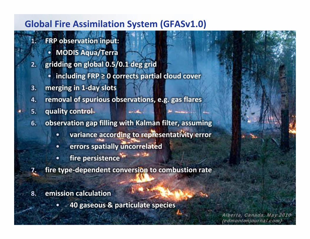
Quality Control: Threshold for Daily FRP Fields

9

MODIS FRP Assimilationobservational coverage proxy FRP

night‐timeobservations

daytimeobservations

24‐houranalysis

10

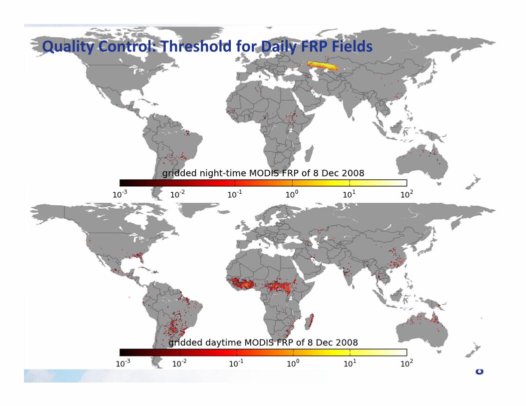
Conversion factor depends on dominant fire type!

FRP conversion factor analysis against GFEDv3

(adapted from Heil et al., ECMWF TM628, 2010)

SA: savannah fires SAOM: SA with potential OM burningAG: agricultural fires AGOM: AG with potential OM burningDF: tropical fires PEAT: peat burningEF: extra-tropical firesEFOM: EF with potential OM burning

SA SAOM AG AGOM DF PEAT EF EFOM

SAOMSA

AGOMAG

PE TF

EFOMEF

MODIS-FRE (PJ month-1)

GFE

D3

DM

(Tg

DM

mon

th-1

)

0

5

10

15

20

25

30

0 5 10 15 20 25 30

0

100

200

300

400

500

0 100

200

300

400

500

0

5

10

15

20

25

30

0 5 10 15 20 25 30

0

5

10

15

20

25

30

0 5 10 15 20 25 30

0

100

200

300

0 100

200

300

0

100

200

300

0 100

200

300

0

100

200

300

0 100

200

300

0

10

20

30

40

0 10 20 30 40

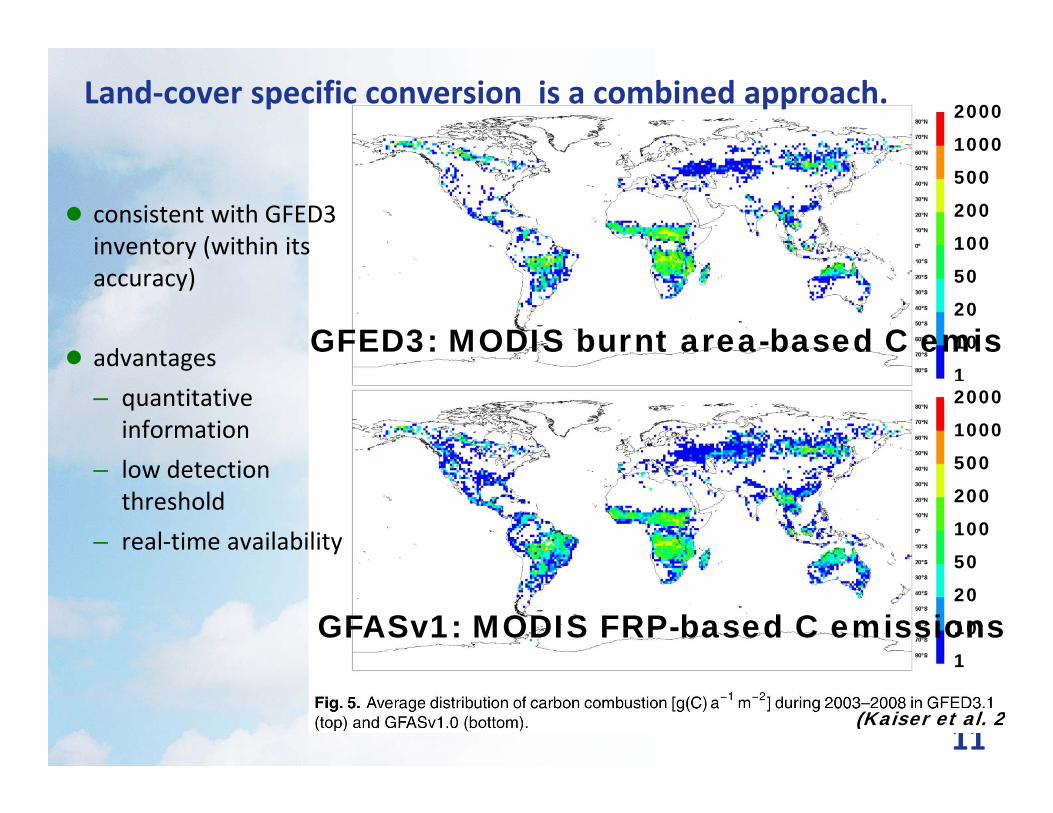
11

2000

1000

500

200

100

50

20

10

12000

1000

500

200

100

50

20

10

1

(Kaiser et al. 2

GFED3: MODIS burnt area-based C emiss

GFASv1: MODIS FRP-based C emissions

consistent with GFED3 inventory (within its accuracy)

advantages– quantitative 

information– low detection 

threshold– real‐time availability

Land‐cover specific conversion  is a combined approach.

12

Comparison to other inventories: Monthly CO emissions

by Niels Andela

13

Black Carbon Cross‐validation

GFASv1.0 (with aerosol enhancement) compares well with NASA’s QFEDv2.2.

(courtesy A. da Silva)

14

Two approaches, with consistent results:Ichoku, da Silva, Sofiev

scale FRP empirically to emissions as observed in plumes

geographical dependence

possibly extend to other species with relative emission factors

Wooster, Kaiser

scale FRP to DM as prescribed in GFED

fire type dependence

adjust single species emission factors to atmospheric observations

Without CO2 observations, the parameters remain underdetermined 

15

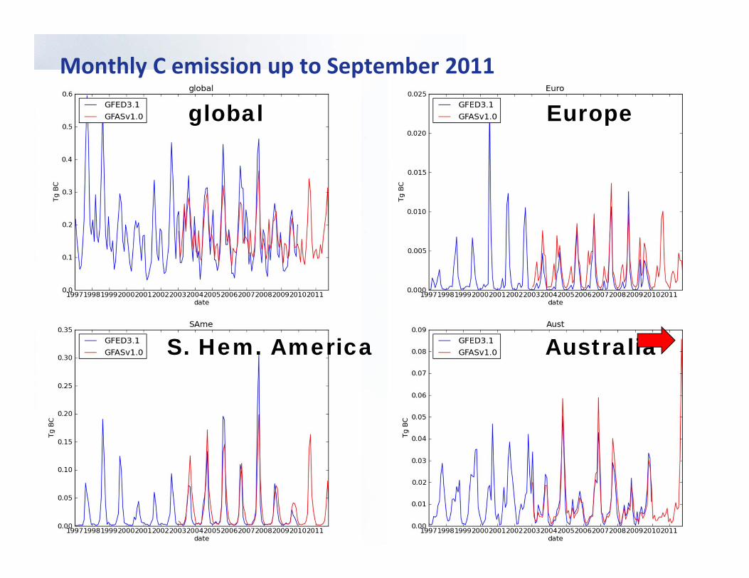
Monthly C emission up to September 2011

global Europe

AustraliaS. Hem. America

16

Monitoring of ECV Fire 

Disturbance

Annual fire anomalies in NOAA’s State of the Climate reports.[Kaiser & van der Werf. BAMS 2010, 2011, 2012, 2013]

anomaly 2009

anomaly 2010

anomaly 2011

anomaly 2012

reduced deforestation

El Nino in late 2010,wet Jan‐Mar 2011/12

SST anomaly in tropical N Atlantic

hot/dry

climate 2003‐2011

17

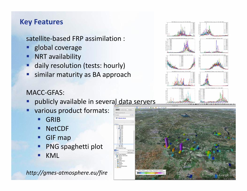
Key Features

satellite‐based FRP assimilation : global coverage NRT availability daily resolution (tests: hourly) similar maturity as BA approach

MACC‐GFAS: publicly available in several data servers various product formats: GRIB NetCDF GIF map PNG spaghetti plot KML

http://gmes‐atmosphere.eu/fire

18

Real‐time Supply Chain

Data providers: (acquired by OBS) NASA: MODIS FRP EUMETSAT LSASAF: SEVIRI FRP

UCAR: GOES‐E/‐W rad. ECMWF: met. forecasts

MACC FRP processing: KCL (IM): GOES‐E/‐W FRP

MACC GFAS processing: GFAS @ ECMWF assimilated FRP combustion rate emissions (injection heights)

archives@ ECMWF: ECFS MARS

archive@ FZJ: OGC web server

GEIA archive: OGC web server

USE

RS

19

Conclusions MACC GFAS is producing

daily biomass burning estimates– for 40 smoke constituents– in real time– publicly available

All global MACC systems consistently use GFAS emissions. More and more regional air quality systems use GFAS. GFAS compares well with other inventories. Feedback from atmospheric validation is becoming more widely available. Many uncertainties remain. Current developments focus on

– plume rise model– merging of geostationary FRP observations– 5‐day fire evolution prediction– improved emission factor formulation

http://gmes‐atmosphere.eu/fire

20

FRP production in MACC

GOES-East Imager

GOES-West Imager

Observational FRP Coverage average number of observations

– damped for large VA of any area in 0.5 deg grid cell during 1 day

Meteosat-9/10 SEVIRIFRP production by EUMETSAT LSA SAF

Terra MODIS

Aqua MODISFRP production by NASA

24096

2462

10.5

[Kaiser et al. 2011]

21

GEO-basedGBBEP-Geo (2010)[Zhang et al. JGR 2012]

LEO-basedGFASv1.0 (2010)[Kaiser et al. BG 2012]

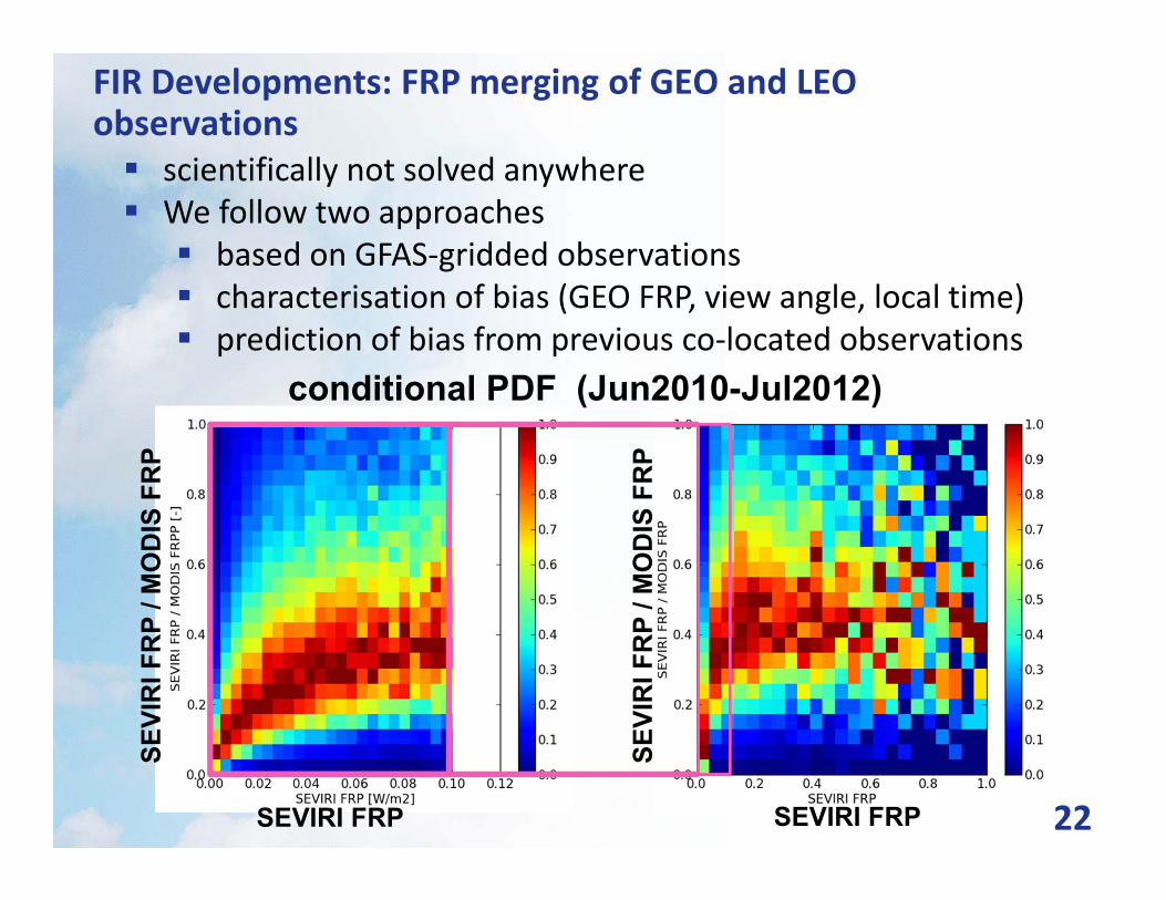
22

conditional PDF (Jun2010-Jul2012)

SEVIRI FRP

SEVI

RI F

RP

/ MO

DIS

FR

P

FIR Developments: FRP merging of GEO and LEO observations scientifically not solved anywhere We follow two approaches based on GFAS‐gridded observations characterisation of bias (GEO FRP, view angle, local time) prediction of bias from previous co‐located observations

SEVIRI FRP

SEVI

RI F

RP

/ MO

DIS

FR

P

23

GFAS Emissions in MACC Systems

– global production

• aerosols

• reactive gases

• greenhouse gases

– reanalysis (2009‐10)

– CO‐tracer forecasts

– EURAD regional forecasts

24

25

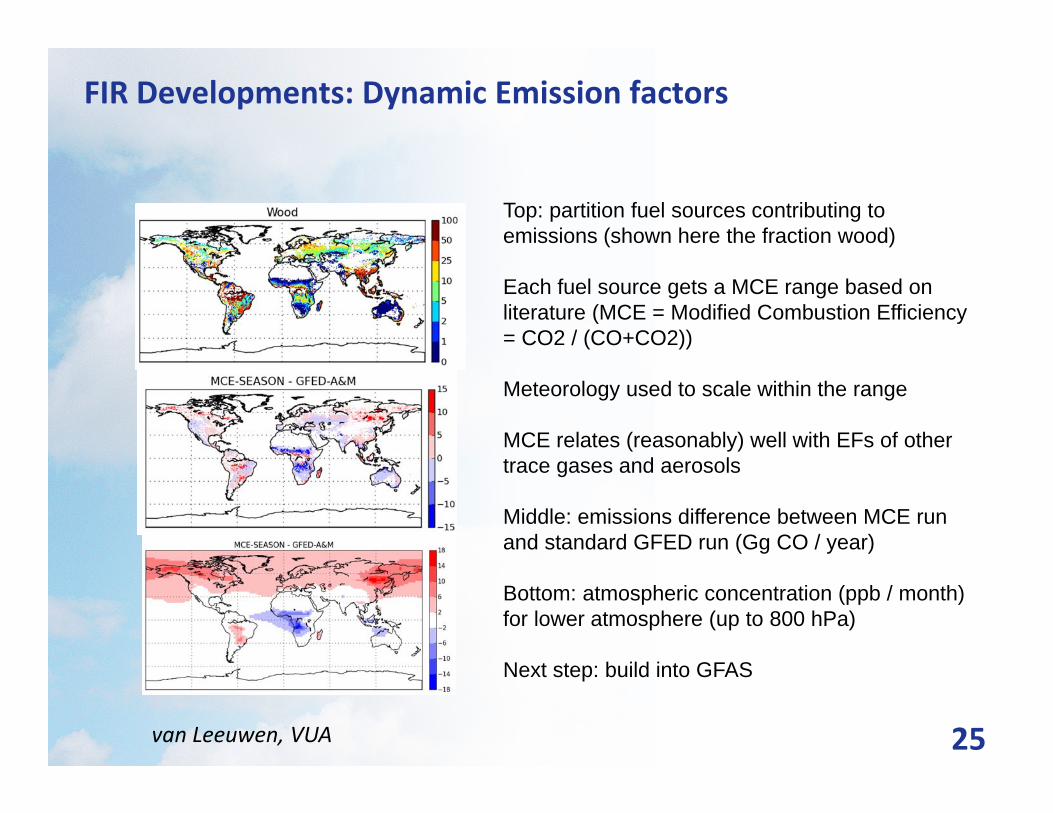
FIR Developments: Dynamic Emission factors

Top: partition fuel sources contributing to emissions (shown here the fraction wood)

Each fuel source gets a MCE range based on literature (MCE = Modified Combustion Efficiency = CO2 / (CO+CO2))

Meteorology used to scale within the range

MCE relates (reasonably) well with EFs of other trace gases and aerosols

Middle: emissions difference between MCE run and standard GFED run (Gg CO / year)

Bottom: atmospheric concentration (ppb / month) for lower atmosphere (up to 800 hPa)

Next step: build into GFAS

van Leeuwen, VUA

26training dataset

Plume Rise Model Development

• MISR reference dataset of observed FRP and plume top height created (N America)

• PRM by Freitas et al. 2007 implemented and optimised

• input data stream from ECMWF operational forecasts

• Sofiev et al. 2012 implemented

• PRMv1 delivered to ECMWF

• for implementation in GFAS

Ronan Paugam, KCL

27

GFAS test version with 1 hour time resolution implemented

assimilation of GOES FRP products 1‐hour forecast based on corresponding 5 hour window of past 24 hours provided for SAMBBA campaign in real time evaluation to follow

28

Key Features

satellite‐based FRP assimilation : global coverage NRT availability daily resolution (tests: hourly)

well documented publicly available in several data servers various product formats: GRIB NetCDF GIF map PNG spaghetti plot KML

http://gmes‐atmosphere.eu/fire

29

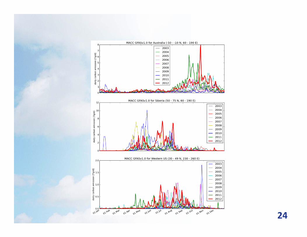
2012 is most interesting: Siberia, Western US & Australia!

30

FRP Example: Russia 2010

July August

carbon combustion rateon 4 August (g d-1 m-2)

31

2010 fires over Russia

Jul-Aug 2010

2007-2010

Fire radiative power from MODIS, east of Moscow (50-60N, 35-

Large night-time values are

indicative of peat fires

Modelled emissions were those appropriate to

woodland fires

Day (04-16UTC)Night (16-04UTC)

32

User statistics: GEIA ECCAD

1. Patricia Oliva, Universidad de Alcala, Spain

2. Giuseppe Baldassarre, Istanbul Technical University, Turkey

3. Taichu Tanaka, Meteorological Research Institute, Japan Meteorological Agency, Japan

4. Koizumi Satoru,,Meteorological Research Institute, Japan Meteorological Agency, Japan

5. Kristofer Lasko,University of Maryland ‐ Department of Geography, Laboratory of Global Remote Sensing Studies, United States

6. Piyush Bhardwaj , Aryabhatta Research Institute of Observational Sciences, India

7. Rodriguez Armando, Fundacion Amigos de la Naturaleza, Bolivia

32