Johannes Spinnewijn

Unemployed but optimistic: optimal insurance design with biased beliefs Article (Accepted version) (Refereed)

Original citation: Spinnewijn, Johannes (2015) Unemployed but optimistic: optimal insurance design with biased beliefs. Journal of the European Economic Association, 13 (1). pp. 130-167. ISSN 1542-4766 DOI: 10.1111/jeea.12099 © 2014 European Economic Association This version available at: http://eprints.lse.ac.uk/59165/ Available in LSE Research Online: April 2016 LSE has developed LSE Research Online so that users may access research output of the School. Copyright © and Moral Rights for the papers on this site are retained by the individual authors and/or other copyright owners. Users may download and/or print one copy of any article(s) in LSE Research Online to facilitate their private study or for non-commercial research. You may not engage in further distribution of the material or use it for any profit-making activities or any commercial gain. You may freely distribute the URL (http://eprints.lse.ac.uk) of the LSE Research Online website. This document is the author’s final accepted version of the journal article. There may be differences between this version and the published version. You are advised to consult the publisher’s version if you wish to cite from it.

Unemployed but Optimistic:

Optimal Insurance Design with Biased Beliefs

Johannes Spinnewijn∗, †

London School of Economics and CEPR

January 20, 2014

Abstract

This paper analyzes how biased beliefs about employment prospects affect the optimal design

of unemployment insurance. Empirically, I find that the unemployed greatly overestimate how

quickly they will find work. As a consequence, they would search too little for work, save

too little for unemployment and deplete their savings too rapidly when unemployed. I analyze

the use of “suffi cient-statistics”formula to characterize the optimal unemployment policy when

beliefs are biased and revisit the desirability of providing liquidity to the unemployed. I also find

that the optimal unemployment policy may involve increasing benefits during the unemployment

spell.

Keywords: Biased Beliefs, Unemployment, Optimal Insurance, Moral HazardJEL Classification Numbers: D83, G22, H30

∗Department of Economics, STICERD 32LIF 3.24, LSE, Houghton Street, London WC2A 2AE, United Kingdom(email: j.spinnewijn@lse.ac.uk, web: http://personal.lse.ac.uk/spinnewi/)†I would like to thank the editor George-Marios Angeletos and three referees for their valuable comments and

suggestions. I also thank David Autor, Douglas Bernheim, Tim Besley, Arthur Campbell, Raj Chetty, StefanoDellaVigna, Mathias Dewatripont, Geert Dhaene, Peter Diamond, Florian Ederer, Jesse Edgerton, Laura Feiveson,Tal Gross, Jonathan Gruber, Bengt Holmstrom, Henrik Kleven, Camille Landais, Robert Shimer, Frans Spinnewyn,Jean Tirole, Ivan Werning, Maurizio Zanardi, and seminar participants at MIT, Toulouse School of Economics, TilburgUniversity, Stanford University, Wharton School , Harvard KSG, Chicago Booth, University College London, LondonSchool of Economics, INSEAD, UCLouvain, Maastricht University, Tinbergen Institute, Harvard University, BonnUniversity, Oxford University, Paris School of Economics, UC Berkeley, UC Davis, ECARES, Hebrew University, TelAviv University, IIES, the CEPR PP Sypmosium, the SITE summer workshop, the CESifo and EEA-ESEM meetingsfor helpful comments and discussions.

1 Introduction

Policy makers and insurers face the trade-off between providing insurance against risks and provid-

ing incentives to avoid these risks. This trade-off is central in the design of unemployment policies

(Baily 1978, Chetty 2006). Unemployment insurance aims to protect workers against the loss of

their earnings when unemployed, but also to preserve their incentives to leave unemployment again.

The workers’perceptions regarding their employment prospects should play a crucial role for this

trade-off. They determine how much workers are willing to protect themselves against unemploy-

ment and how much effort displaced workers are willing to invest to find new employment. However,

comparing the reported expectations of unemployed job seekers to the actual outcomes of their job

search reveals a striking optimistic bias. Based on a survey by Price et al. (1998), I find that on

average unemployed job seekers expect to remain unemployed for an additional 6.8 weeks.1 Only

one out of ten job seekers expect that he or she will need more than three additional months to

find employment. In follow-up interviews, subjects are asked when they actually started working.

Accounting for censored unemployment spells, the average remaining duration for the same sample

of job seekers exceeded 23.0 weeks. This is more than three times longer than expected. One out

of two job seekers needed more than three additional months to find employment. This remarkable

optimistic bias is also illustrated in Figure 1 showing the distribution of the difference between the

actual and expected remaining duration of unemployment for the different job seekers: more than

80% of the job seekers have underestimated rather than overestimated the length of their unem-

ployment spell and their forecast errors are much more pronounced. This evidence complements a

large empirical literature in psychology and economics documenting systematic biases in risk per-

ceptions and motivates analyzing the role of biased beliefs for the optimal design of unemployment

insurance. The analysis in this paper shows that the presence of biased beliefs affects the conclu-

sions regarding two prominent topics in the recent literature: the first regards the identification of

"suffi cient statistics" capturing the optimal trade-off between insurance and incentives, the second

regards the optimal timing of unemployment benefits and the optimal provision of liquidity.

I first consider a stylized model of unemployment (Baily 1978, Chetty 2006) in which an em-

ployed agent decides how much to save for unemployment and how much to search when unem-

ployed. In contrast with previous work, I allow the agent to have biased beliefs about her em-

ployment prospects and to maximize her perceived expected utility. A paternalistic social planner,

however, designs the unemployment policy to maximize the agent’s true expected utility. When

determining the optimal generosity of the unemployment policy, the social planner trades off the

value of additional insurance and the cost of reduced incentives. This trade-off depends critically

on how beliefs are biased in two particular dimensions. The baseline beliefs - the beliefs about the

baseline job finding probability for given search efforts - affect the perceived value of insurance and

1The results are based on a sample of 1,487 job seekers in Michigan and Maryland surveyed repeatedly between1996 and 1998 by Price et al. (1998). Subjects were asked about their baseline expectations in the question: "Howmany weeks do you estimate it will actually be before you will be working more than 20 hours as week." I providemore details about the survey, the empirical results and the robustness of the optimistic bias in the appendix.

2

Figure 1: Histogram of differences between actual and expected unemployment durations. Calculations arebased on a survey by Price et al. (1998).

thus the agent’s willingness to save for unemployment. The control beliefs - the beliefs about the in-

crease in the job finding probability when searching more intensively - affect the agent’s willingness

to exert search effort in order to leave unemployment.

I characterize the impact of these biases on the optimal unemployment policy by building on a

canonical result known as the Baily formula. In its standard formulation, this formula states that

at the optimum the consumption smoothing benefit from an increase in unemployment benefits

should be equal to the incentive (or moral hazard) cost. The consumption smoothing benefit

depends on the wedge between employment and unemployment consumption, while the incentive

cost is captured by the elasticity of the unemployment probability. Several recent studies have

analyzed the implementation of the Baily formula as it identifies two simple suffi cient statistics for

unemployment policy that can be estimated using reduced-form methods (see Gruber 1997, Chetty

2006, 2008, 2009, Shimer and Werning 2007, Landais 2013). A key insight of the suffi cient-statistics

analysis is that the agent’s behavioral responses to policy only matter to the extent that they affect

the policy maker’s budget. This is no longer true when an agent’s behavior is distorted due to

biased beliefs. Biased beliefs do not only change the consumption wedge and the elasticity of the

unemployment probability that we would estimate empirically, but also make that corrections of

these respective statistics are required to characterize the optimal policy. While the moral hazard

cost needs to be corrected for the distortion in search efforts, the consumption smoothing benefit

needs to be corrected for the distortion in precautionary savings. The analysis reveals the potential

value of active labor market policies affecting search efforts directly and the potential cost of policies

relying on the individuals’own savings to protect themselves against unemployment (e.g., Altman

and Feldstein 2006).

I then consider a standard dynamic model of the unemployment spell (Shavell and Weiss 1979,

Hopenhayn and Nicolini 1997) to analyze the dynamics of the unemployment policy. I explicitly

allow for unobservable savings and focus on CARA preferences like in Werning (2002) and Shimer

and Werning (2008). I first use the model to show that the Baily decomposition into consumption

3

smoothing benefits and incentive costs again leads to an intuitive characterization of the optimal

static unemployment policy and the corrections required for biased beliefs in this dynamic model.

I then use the model to analyze the optimal timing of benefits and the desirability of allowing

borrowing and savings. In particular, I revisit the powerful result in Shimer and Werning (2008)

that the optimal unemployment policy can be implemented with a simple policy that keeps un-

employment benefits and taxes constant and gives the unemployed access to savings. This result

assumes unbiased beliefs. A baseline-optimistic agent, however, underestimates how long she will

remain unemployed and will deplete her assets too rapidly given the expected duration of her un-

employment spell. In theory, this increases the value of controlling the unemployed’s savings and

puts into question the (uncontrolled) provision of liquidity to the unemployed. A calibration of

the dynamic model suggests that access to savings substantially increases the value of the static

unemployment policy. This increase hardly depends on whether the access to savings is controlled

or not provided that the static policy is optimally adjusted. Finally, by underestimating the prob-

ability to be long-term unemployed a baseline-optimistic job seeker is also less responsive to future

incentives. As a consequence, the social planner can provide more insurance to the long-term un-

employed at a low incentive cost for the short-term unemployed. I show how this can result in

increasing unemployment benefits during the unemployment spell.

Related Literature A vast literature in psychology starting with the seminal work by Tverskyand Kahneman (1974) and a growing literature in economics find that risk perceptions are subject to

systematic biases. By now there is broad evidence that people tend to overestimate the probability

of positive events and underestimate the probability of negative events.2 This has also lead to a

theoretical literature proposing explanations for the biases in beliefs and finding that optimistic

beliefs are more likely to arise and persist.3 In the context of unemployment, some previous work

has analyzed perceptions about employment prospects, but without linking the perceptions and

outcomes of the same individuals (see Manski 2004). A recent poll by Gallup in the US finds that 4

in 10 unemployed job seekers expect to find employment within a month. The average job finding

rate in the US is, however, much lower, which is again suggestive of a substantial optimistic bias.4

In ongoing work, Mueller and Spinnewijn analyze how perceptions evolve during the unemployment

spell using a survey of job seekers in New Jersey during the most recent recession. They find an

optimistic bias that is as extreme in magnitude and persists during the unemployment spell.

The analysis in this paper fits well in the behavioral public economics literature, studying

optimal policies with non-standard decision makers.5 First, behavioral biases like biases in beliefs2Moore and Healy (2008) provide an excellent overview. For seminal contributions, see for example Weinstein

(1980) and Slovic (2000). De Bondt and Thaler (1995) conclude: "Perhaps the most robust finding in the psychologyof judgment is that people are overconfident." In this literature, overconfidence is often interpreted as over-estimationof a probability relative to the true probability, which relates to my definition of baseline-optimism. However, it canalso refer to over-placement (i.e., the belief that one performs better than others) and over-precision (i.e., the beliefthat one’s information is more precise than it actually is).

3Examples are Gervais and Odean (2001), Bénabou and Tirole (2002 and 2006), Compte and Postlewaite (2004),Van den Steen (2004), Brunnermeier and Parker (2005), Gollier (2005) and Köszegi (2006).

4See http://www.gallup.com/poll/145817/Unemployed-Americans-Face-Challenging-Job-Search.aspx.5For reviews, see Kanbur et al. (2006), Bernheim and Rangel (2007) and Mullainathan et al. (2012).

4

distort behavior and thus affect the need for public policies and their impact. In the context

of unemployment, DellaVigna and Paserman (2005) have analyzed theoretically how impatience

distorts job search behavior. Paserman (2008) has estimated the discounting process to evaluate

particular policy interventions numerically. Second, behavioral biases affect how observed behavior

needs to be interpreted when designing policies. The characterization of the Baily formula adjusted

for biased beliefs adds to the recent literature, reviewed by Chetty (2009), analyzing conditions

under which suffi cient statistic formulas for taxation and social insurance apply or need to be

adjusted. The empirical estimation of the bias in beliefs helps to identify agents’true preferences

from their observed choices, as argued by Köszegi and Rabin (2007 and 2008). Finally, behavioral

biases may justify government intervention in insurance markets. Cutler and Zeckhauser (2004)

have argued that people’s poor understanding of risk and insurance choices is one of the reasons

for the divergence between insurance theory and insurance practice. In other contexts, previous

work has focused on the response by private firms to behavioral biases and the potential welfare

consequences (see Ellison 2006, DellaVigna 2009). In particular, Santos-Pinto (2008) and De la

Rosa (2011) analyze the change in incentive contracts proposed by a profit-maximizing principal

in response to specific optimistic biases.6

The paper is organized as follows. Section 2 sets up a stylized two-period model and defines the

baseline and control beliefs. Section 3 derives an adjustment of the Baily formula characterizing

the optimal policy in the presence of biased beliefs. Section 4 introduces a dynamic model of the

unemployment spell and analyzes the features of the optimal policy in a dynamic context. Section

5 calibrates this dynamic model and provides some numerical explorations of the optimal policy

features and its welfare consequences. Section 6 concludes. All proofs are presented in appendix.

2 Stylized Model

I first consider a two-period model that closely follows the seminal model of unemployment by Baily

(1978). A risk-averse agent is employed in the first period, but faces the risk to be unemployed in

the second period. In the first period, the agent decides how much to save to protect herself against

the loss of earnings when unemployed. In the second period, the agent decides how hard to search

for employment.

In each period, the agent earns a wage w when employed and 0 when unemployed. In the first

period, the agent can save s ∈ [0, w] to increase her consumption in the second period by (1 + r) s,

regardless of her employment status. In the second period, the agent finds work with probability

π (e) ∈ [0, 1] when exerting search effort at utility utility cost e ≥ 0. The job finding probability

is increasing, but concave in the search cost, π′ (e) ≥ 0, π′′ (e) < 0. For notational convenience, I

assume that the agent is certain to lose her job after the first period and is thus obliged to search

6A different set of papers focuses on the impact of heterogeneity in risk perceptions on the design of insuranceor other contracts. See for example Sandroni and Squintani (2007), Eliaz and Spiegler (2008), Grubb (2009) andSpinnewijn (2012, 2013).

5

for a new job in the second period.7

The social planner provides mandatory insurance against the unemployment risk. The agent

receives a benefit b when unemployed, but pays a tax τ when employed. The insurance reduces

the wedge between employment and unemployment consumption. The policy cannot be made

conditional on the agent’s behavior, but affects how much she saves when employed in the first

period and how much search effort she exerts after being displaced in the second period. The

expected utility of an unemployment policy (b, τ) for an agent with Bernouilli-utility function u (·)and discount factor β who saves s and exerts effort e equals

u(w − τ − s) + β [π (e)u(w − τ + (1 + r) s) + (1− π (e))u(b+ (1 + r) s)− e] .

I will use c0, ce and cu as short-hands of the consumption levels in the first period of employment,

the second period when employed and the second period when unemployed respectively.

2.1 Biased Beliefs

The agent’s behavior depends on her perceived employment prospects. I allow the agent’s be-

lief regarding her job finding probability to be different from the true probability. I denote by

π (e) ∈ [0, 1] the agent’s belief when exerting effort e. Like the true probability π (e), the perceived

probability π (e) is increasing and concave in e. I deliberately put no other restrictions on how the

true and perceived probability are related. The analysis, however, will show that the difference is

essential in two dimensions; the difference in levels π (e)−π (e), the baseline bias, and the difference

in margins π′ (e)− π′ (e), the control bias.

Definition 1 An agent is baseline-optimistic (-pessimistic) if π (e) ≥ (≤) π (e)for all e ≥ 0.

Definition 2 An agent is control-optimistic (-pessimistic) if π′ (e) ≥ (≤) π′ (e) for all e ≥ 0.

Baseline and control beliefs are interdependent. Whether baseline-optimistic agents are also

more optimistic about their control may depend on the context, as illustrated by the following two

examples constructed by using an increasing, but concave function ρ (e).8

Example 1: π (e) = θ × ρ (e) and π (e) = θ × ρ (e); the probability of finding work is comple-

mentary in the job seeker’s ability θ and effort e. A job seeker who overestimates her ability (i.e.,

θ > θ) is at the same time baseline-optimistic and control-optimistic.

Example 2: 1 − π (e) = φ × [1− ρ (e)] and 1 − π (e) = φ × [1− ρ (e)]; a job seeker who

underestimates the probability to remain unemployed when exerting no search effort (i.e., φ < φ)

will be baseline-optimistic, but will also underestimate the return to reducing this probability by

searching and thus be control-pessimistic.7For notational convenience, I do not consider the possibility that the worker retains her job, which would introduce

an additional state. Still, an alternative interpretation of the model is that the agent exerts effort to keep her job inorder to capture moral hazard on-the-job.

8Note that the theoretical results apply for any baseline and control bias. For expositional purposes, I do restrictattention to biases in beliefs that are the same for all effort levels, although only the bias in beliefs evaluated at thechosen effort level will matter.

6

2.2 Agent’s Problem

The agent chooses an effort level e and savings level s to maximize her perceived expected utility

taking the unemployment policy (b, τ) as given,

U (b, τ) = maxe,s

u(w − τ − s) + β [π (e)u(w − τ + (1 + r) s) + (1− π (e))u(b+ (1 + r) s)− e] .

At an interior solution, the levels equalize the respective perceived individual benefit and cost at

the margin,

π′ (e) [u(ce)− u(cu)]− 1 = 0, (ICe)

−u′ (c0) + β (1 + r){π (e)

[u′(ce)− u′(cu)

]+ u′(cu)

}= 0. (ICs)

From ICe, it follows that the agent exerts more effort the higher she perceives the marginal

return to effort to be. As a consequence, her effort and thus her probability of finding work is

higher when she is control-optimistic than when she is control-pessimistic. This is true as long as

the consumption wedge ce− cu is positive. The more insurance the unemployment policy provides,the smaller the consumption wedge. The agent responds by decreasing her search effort and more

so if she is control-optimistic.

From ICs, it follows that the agent saves less the higher she perceives the job finding probability

to be. This is true as long as the consumption wedge ce−cu is positive by concavity of the Bernouilliutility. In contrast with the effort choice, the consumption choice depends on the baseline beliefs. A

baseline-optimistic agent underestimates the value of unemployment insurance and protects herself

less against the unemployment risk through precautionary savings. The less the unemployment

policy insures the agent against the loss of earnings, the larger her incentive to save.9

3 Optimal Unemployment Policy

The social planner faces the trade-off between providing insurance and maintaining incentives for

search. The agent’s perception of her employment prospects is central to this trade-off.

3.1 Social Planner’s Problem

The expected expenditures and revenues for the social planner depend on the agent’s true em-

ployment probabilities. I assume that the social planner is paternalistic and also uses these true

probabilities to weight the different states when calculating the agent’s expected utility.10 While

9Since the earnings distribution in the second period is first-order stochastically dominated by the earnings inthe first period, u′′′ > 0 is not necessary to explain precautionary savings for the unemployment risk. By implicitdifferentation of ICs, it follows that the savings level increases in response to a decrease in b (i.e., dsdb < 0) regardlessof the sign of u′′′. For the savings level to increase in response to a decrease in τ , u′′′ > 0 is not necessary either, butsuffi cient.10The insights generalize for welfare concepts putting some positive weight on the agent’s perceived expected utility.

In the web-appendix, I contrast the optimal policy under this extreme welfare criterion with the policy implemented

7

only the true probabilities enter the social planner’s problem directly, they still depend on the

agent’s behavior and thus on the agent’s beliefs. I assume that the social planner knows the agent’s

beliefs, which cannot be manipulated, nor changed in response to the unemployment policy.11

Hence, the social planner solves

maxb,τ

u(w − τ − s) + β [π (e)u(w − τ + (1 + r) s) + (1−π (e))u(b+ (1 + r) s)− e]

subject to ICe, ICs and

τ +1

1 + r[π (e) τ − (1− π (e)) b] = 0. (BC)

I denote the agent’s true expected utility by U (b, τ) and the social planner’s profit by P (b, τ). For

any unemployment benefit level b, the incentive compatibility constraints and the budget constraint

implicitly determine a tax level τ (b), an effort choice e (b) and a savings choice s (b). I assume that

these functions are well-behaved for the relevant range of values for b with τ ′ (b) > 0, e′ (b) ≤ 0 and

s′ (b) ≤ 0 and drop the argument when it is clear.

For the unemployment policy to be optimal, a budget-balanced increase in the unemployment

benefit b cannot increase the agent’s welfare,

dU

db= 0 ⇔ ∂U

∂b+∂U

∂ττ ′ (b) +

∂U

∂ee′ (b) +

∂U

∂ss′ (b) = 0. (1)

An increase in the unemployment benefit b has three types of effects. First, it directly increases

the agent’s utility when unemployed. Second, it requires an increase in the tax to keep the budget

balanced and thus affects the agent’s utility when employed. Third, it changes the agent’s behavior:

the agent reduces her search effort e and her savings s. With unbiased beliefs, these behavioral

responses have only a second-order impact on the agent’s expected utility by the envelope condition.

That is, if the agent were to maximize her true expected utility, the last two terms in equation

(1) would drop and the social planner could ignore the utility impact of any behavioral response.

This is a key force in the analysis by Baily (1978) and the suffi cient statistic literature in public

economics (see Chetty 2006, 2009). However, this no longer applies when an agent has biased

beliefs and maximizes her perceived rather than her true expected utility.

I relate the first-order utility impact of these behavioral responses when beliefs are biased to the

standard moral hazard cost and consumption smoothing benefit from an increase in unemployment

benefits.

Moral Hazard: Perceived Returns to Search Higher unemployment benefits lower the in-

centives for an unemployed agent to search for work. Moral hazard arises as the agent does not

internalize the impact of her effort on the social planner’s expected revenues and expenditures.

by a populist government catering to its voters’beliefs. Such government would propose the same policy as profit-maximizing insurers in a competitive equilibrium. I briefly discuss this in Section 3.3.11These assumptions correspond to a setting with different priors where the social planner and the agent ‘agree to

disagree’.

8

The tax increase required to balance the budget is larger the more responsive the agent’s search

effort. The impact of this behavioral response on the social planner’s budget is fully captured by

the elasticity of the unemployment probability with respect to a budget-balanced increase in the

unemployment benefit. That is, the required tax increase equals

τ ′ (b) =τ (b)

b

[1 + ε1−π(e),b

], with ε1−π(e),b ≡

d (1− π (e (b)))

db

b

1− π (e (b)). (2)

The higher the elasticity, the worse the rate at which the social planner can transfer consumption

from employment to unemployment and thus the more costly it is to provide insurance against

unemployment.

The agent’s biased beliefs introduce a second externality related to her effort choice, which I

refer to as a search internality. If the perceived and true marginal return to search differ, the agent

does not correctly internalize the effect of her search effort on her true expected utility. The social

planner affects this search internality when changing the unemployment policy. Using ICe, I find

∂U

∂ee′ (b) = β

[π′ (e)− π′ (e)

][u(ce)− u(cu)] e′ (b) . (3)

With unbiased control beliefs, this effect is of second order. However, when the agent is control-

pessimistic, π′ (·) > π′ (·), she underestimates the marginal return to effort and exerts too little effortgiven the true return. A decrease in her effort choice in response to an increase in unemployment

benefits now causes a first-order decrease in welfare. When the agent is control-optimistic, the

opposite happens. In fact, the positive search internality due to her control-optimistic beliefs may

offset the negative externality due to moral hazard and thus reduce the incentive cost from providing

unemployment insurance.

Consumption Smoothing: Perceived Value of Insurance Unemployment benefits provide

insurance by reducing the wedge between employment and unemployment consumption. The wel-

fare gain from a budget-balanced increase in the unemployment benefit is increasing in the wedge

between the marginal utility of consumption when employed and unemployed. Ignoring behavioral

responses, the normalized utility gain equals

[∂U

∂b+∂U

∂τ

τ (b)

b]/[−∂U

∂τ

τ (b)

b] =

u′ (cu)− u′ (ce)u′ (ce)

, (4)

for β (1 + r) = 1 and u′ (ce) ≡ [u′ (c0) + βπ (e)u′ (ce)] / [1 + βπ (e)] denoting the average (dis-

counted) marginal utility when employed. The relative difference in marginal utilities and thus the

consumption smoothing benefit of the unemployment policy is decreasing in the benefit b and tax

τ .

Higher unemployment benefits also reduce the gains from self-protection against the unem-

ployment risk. The social planner’s unemployment policy crowds out the agent’s precautionary

savings. The welfare impact of the crowd-out response when considering a marginal change in the

9

unemployment policy is again of second order if agents have unbiased beliefs. Using ICx, I find

∂U

∂ss′ (b) = β (1 + r) [π (e)− π (e)]

[u′(cu)− u′(ce)

]s′ (b) . (5)

When the agent is baseline-optimistic about her employment prospects, π (e) > π (e), she saves

too little to protect herself against unemployment. A further decrease in her precautionary savings

in response to an increase in the unemployment benefit thus causes a first-order decrease in her

expected utility.

3.2 Adjusted Baily Formula

Using the above expressions, the optimality condition (1) can be rewritten to find a Baily formula

adjusted for biased beliefs. The formula states that when setting unemployment benefits the gain

from providing insurance and the cost from reducing the search incentives have to be equalized at

the margin.

Proposition 1 The optimal unemployment policy is characterized by

u′(cu)− u′ (ce)u′ (ce)

[1− π (e)− π (e)

1− π (e)I (b)

]= ε1−π(e),b

[1− π′ (e)− π′ (e)

π′ (e)J (b)

], (6)

for I (b) = −u′(cu)−u′(ce)u′(cu)−u′(ce)

s′(b)β ≥ 0, J (b) = u(ce)−u(cu)

bu′(ce)≥ 0 and β (1 + r) = 1.

When beliefs are unbiased, condition (6) simplifies to the standard Baily formula12,

u′ (cu)− u′ (ce)u′ (ce)

= ε1−π(e),b. (7)

This formulation by Baily (1978) is central in the recent literature in public finance developing and

implementing “suffi cient statistic formulas”for social insurance (Chetty 2009). The Baily formula

suggests that the identification of two moments is suffi cient to guide policy design. If the relative

difference in marginal utilities exceeds the elasticity ε1−π(e),b, an increase in the unemployment

benefit increases welfare. The larger the difference in marginal utilities or the smaller the elasticity,

the higher the expected welfare gain. Identifying the primitives underlying the agent’s search and

savings decision is not necessary. The appeal of this approach is thus that policy recommendations

can be based on a small set of high-level empirical moments, which have been credibly estimated in

the empirical literature.13 However, when biased beliefs distort a job seeker’s behavior, the Baily

formula prescribes an unemployment benefit level that is generally suboptimal. The direction

12Note that the second order condition of the social planner’s maximization problem requires that u′(cu)−u′(ce)u′(ce)

decreases more in b than ε1−π(e),b.13A large literature has analyzed the unemployment responses to unemployment benefits (see Krueger and Meyer

(2002) for a review). Gruber (1997) estimates the relative difference in consumption when employed and unemployedto approximate the relative difference in marginal utilities, i.e., [u′ (cu)− u′ (ce)] /u

′ (ce) ∼= γ∆ccfor relative risk

aversion parameter γ. See Shimer and Werning (2007) and Chetty (2008) for alternative implementations.

10

in which the benefit level should be adjusted depends only on the belief biases as illustrated in

Corollary 1 and 2.

Corollary 1 The elasticity ε1−π(e),b overestimates (underestimates) the cost from reducing incen-

tives when agent’s have control-optimistic (-pessimistic) beliefs.

The cost from reduced incentives depends on both the moral hazard cost and the search inter-

nality. The search internality appears as a correction of the elasticity in the adjusted Baily formula

(6), which depends on the control bias. Ignoring this correction would lead the social planner to set

the unemployment benefit suboptimally high for control-pessimistic agents and suboptimally low

for control-optimistic agents. Note that the social planner can correct the search internality only to

the extent that the agent is responsive to its policy. In case of a zero elasticity, for example when

the job seeker believes she has no control over her situation, she will not respond to changes in the

unemployment benefits. This indicates the potential importance of other unemployment policies

to encourage search directly, like job search monitoring and job search assistance. The impact of

biased control beliefs on the optimal benefit level itself is also ambiguous despite the unambiguous

correction in the formula. The reason is that control beliefs also affect the standard moral hazard

cost (by changing the responsiveness and thus the elasticity ε1−π(e),b) and consumption smoothing

benefits (by changing effort and thus the required tax τ (b)) with potentially opposite effects on

the optimal benefit level. This can be easily seen when the control beliefs are either extremely

pessimistic or optimistic, since in both cases the optimal policy converges to full insurance (i.e.,

ce − cu → 0).14

Corollary 2 The relative difference [u′ (cu)− u′ (ce)] /u′ (ce) overestimates (underestimates) thegain from providing insurance when agents have baseline-optimistic (-pessimistic) beliefs.

The gain from providing additional insurance depends on the relative difference in marginal

utilities, but needs to be corrected for the crowd-out of savings when beliefs are biased. The

correction depends on the baseline bias. Note that baseline-optimistic agents save less to protect

themselves against the unemployment risk and thus gain more from higher unemployment benefits.

This is reflected by the higher relative difference in marginal utilities due to the lower savings.

However, this relative difference overstates the welfare gain from increasing unemployment benefits.

This is due to the reduction in savings in response to the benefit increase, although the savings are

already insuffi cient. Similarly, baseline-pessimistic agent smooth their consumption more and thus

gain less from higher unemployment benefits, but this gain is larger than indicated by the relative

difference in marginal utilities.

14When the agent is extremely pessimistic about her control, the increase in search efforts when introducing a(costly) wedge between employment and unemployment consumption is too low. When the agent is extremelyoptimistic about her control, a small wedge would suffi ce to induce her to exert the effi cient level of search.

11

3.3 Self-Protection against Unemployment

The analysis highlights that workers who overestimate their job finding probability (or underesti-

mate their job loss probability) are expected to save too little and to be unprepared for the loss of

earnings when unemployed. The optimism about employment prospects might explain why many

unemployed individuals have limited liquidity (Chetty 2008) and raises doubts regarding the desir-

ability of individual unemployment savings accounts to provide protection against unemployment

as proposed by Altman and Feldstein (2006). The under-investment and its consequences for opti-

mal policy extend to any type of self-insurance against the unemployment risk that workers could

invest in. As such, the optimistic bias may provide an alternative explanation for the puzzle why

unemployment insurance is almost always publicly provided (Acemoglu and Shimer 2000). This

can be illustrated in an extended model with private insurance. The desirability of social insurance

depends on whether or not the equilibrium coverage provided by private insurers is socially optimal.

Like a social planner, private insurers are constrained by the true employment probabilities when

designing their policies. However, in order to attract agents with biased beliefs, they would offer

policies that maximize the agents’perceived rather than true expected utility. In particular, private

insurers would offer less insurance than is socially optimal in response to the low valuation implied

by baseline-optimistic beliefs. In addition, they would not adjust the coverage to correct for the

distortions in the agent’s search behavior driven by her biased control beliefs. Both effects illustrate

why the well-known result that moral hazard, in contrast with adverse selection, does not raise the

need for government intervention (e.g., Chetty and Saez 2010) holds only if the agent’s beliefs are

unbiased. In the web-appendix to this paper, I show these insights formally by characterizing the

insurance policy provided by private insurers in a competitive equilibrium, which would coincide

with the optimal policy when beliefs are unbiased.15

4 Dynamic Model of the Unemployment Spell

The previous section characterized the optimal generosity of the unemployment policy focusing on

the role of biased beliefs for the incentives for workers to save for unemployment and for displaced

workers to leave unemployment. This section provides a complementary analysis of the role of

biased beliefs for the search and consumption choices of unemployed job seekers during the unem-

ployment spell and also studies the consequence for the optimal dynamics of the unemployment

policy. I consider a standard dynamic model of the unemployment spell in which a job seeker starts

unemployed and decides how much to search for employment as long as she has not found employ-

ment (see Shavell and Weiss 1979, Hopenhayn and Nicolini 1997, Shimer and Werning 2008, etc.).

The job seeker has also access to assets which can be used to increase unemployment consumption

at the expense of future consumption and thus make consumption levels dependent on the length

of the unemployment spell.

15Note that this is also the policy that a non-paternalistic policy maker would propose when trying to gain theagent’s vote in elections.

12

I consider the case of CARA preferences for which Werning (2002) and Shimer and Werning

(2008) show that the social optimum is achieved with constant unemployment benefits and taxes

when job seekers are not liquidity constrained. First, I show how the optimal characterization of

this constant policy generalizes the previous insights of the adjusted Baily formula to this dynamic

setting. Note that both the effort and savings decision will now depend on the perceived length

of the unemployment spell. Baseline-optimistic job seekers search too little and draw down their

assets too quickly given the true expected duration. The latter implies that access to liquidity

is no longer suffi cient to achieve the social optimum. Finally, I also show how the social planner

could increase the welfare of baseline-optimistic agents by increasing the unemployment benefits

and taxes with the length of the unemployment spell.

4.1 Setup

The agent now starts unemployed and exerts effort at cost e to find work. She finds a job with

probability π (e) in a given period, but she believes this probability to be equal to π (e). If the agent

does not find work in a given period, she has to search again in the next period. Once she finds a

job, she remains employed forever.16,17 I assume CARA preferences with the cost of effort expressed

in monetary terms, u (c− e) = − exp (−σ (c− e)). Next to the unemployment benefits and taxes,the agent has also access to a risk-free asset a with interest rate r to smooth her consumption. The

agent’s discount factor equals β with β (1 + r) = 1.

I consider the constant policy (b, τ) specifying the constant benefit b received when unemployed

and the constant tax τ paid when re-employed. An agent with CARA preferences makes her search

and consumption decision based only on differences in income levels. With a constant policy, these

differences remain the same throughout the unemployment spell.

Lemma 1 An agent with CARA preferences facing a constant policy (b, τ) exerts a stationary

effort level e and depletes her asset holdings by a stationary amount x. The perceived continuation

value in unemployment equals

U (b, τ |a) =u (cu (a)− e) + β

1−β π (e)u (ce (a)− rx)

1− β (e, x), (8)

with β (e, x) ≡ β (1− π (e)) exp (σrx).

The stationarity makes the problem particularly tractable and allows for a closed-form expres-

sion for the continuation value in unemployment with a simple interpretation: each period that

16 It is possible to introduce a spell of employment at the start in the spirit of the stylized two-period model. Thiswould confirm the earlier insights and not affect the dynamic results. Note that in the dynamic model effort exertedin a given period of unemployment affects employment in the next period, which is different from the stylized model.17 I assume that job seekers do not learn about their bias during unemployment; both the true probability function

of effort π (e) and the perceived probability function of effort π (e) remain unchanged during unemployment. Inthe web-appendix, I discuss empirical evidence suggesting that the optimistic baseline bias does not decrease duringunemployment.

13

the job seeker starts unemployed she receives a utility flow that depends on her unemployment

utility and the expected utility from potentially becoming employed. This utility flow is discounted

by β (e, x) which in addition to the discount factor β depends on the perceived probability of

unemployment and the rate at which the utility flow decreases through asset depletion.

The agent’s effort level solves

βπ′ (e) exp (σrx)

[u (ce (a))

1− β − U (b, τ |a)

]= u′ (cu (a)− e) . (IC ′e)

Her effort now depends on her baseline beliefs as well. A baseline-optimistic job seeker overesti-

mates the probability of leaving unemployment and thus the continuation value in unemployment

U (b, τ |a). As a consequence, she exerts less effort to leave unemployment. The agent’s consumption

levels during unemployment and upon re-employment equal respectively,

cu (a) =r

1 + ra+ b+ x,

ce (a) =r

1 + ra+ (w − τ) .

The static wedge between employment and unemployment consumption is decreasing in the unem-

ployment benefit and the tax as in the two-period model. A job seeker can now decrease this static

wedge by running down her savings at the expense of future consumption. That is, when increasing

today’s unemployment consumption by x, it is optimal to reduce all future consumption levels by

rx, whether employed or unemployed. The reduction of the static wedge by x thus introduces a

dynamic wedge rx measuring the slope of the decreasing profile of unemployment consumption.

The job seeker trades off this static and dynamic wedge and sets x to solve

u′ (cu − e)− u′ (ce)u′ (cu − e)

=1

π (e)

(1− 1

exp (σrx)

), (ICx)

where 1/π (e) equals the job seeker’s belief regarding the expected duration of her unemployment

spell. The left-hand side captures the value of a reduction in the static wedge, while the right-hand

side captures the cost from an increase in the dynamic wedge. The shorter a job seeker expects to

remain unemployed, the more willing she is to run down her savings during unemployment in order

to reduce the static wedge.

4.2 Adjusted Baily Formula

The social planner again sets the benefit level of a budget-balanced policy to maximize the agent’s

true expected utility, constrained by the agent’s effort and consumption choices. Budget balance

for a constant policy simplifies to τ = rb/π (e). The required tax to balance the budget is higher

the longer the true expected duration of the unemployment spell 1/π (e). Like in the two-period

model, the constraints implicitly define three functions τ (b) , e (b) and x (b) and the optimal benefit

14

level b satisfiesdU

db= 0 ⇔ ∂U

∂b+∂U

∂ττ ′ (b) +

∂U

∂ee′ (b) +

∂U

∂xx′ (b) = 0. (9)

This condition allows for a Baily-type characterization of the optimal constant policy in this dy-

namic setting. Note that at the optimum both the search effort and the depletion level are de-

creasing in response to a budget-balanced increase in the unemployment benefit, i.e. e′ (b) ≤ 0 and

x′ (b) ≤ 0.

Proposition 2 With CARA preferences, the optimal constant policy is characterized by

u′ (cu − e)− u′ (ce − rx)

u′ (ce − rx)

{1 +

π (e)− π (e)

1− π (e)K (b)

}= ε1/π(e),b

{1− (1− π′ (e)

π′ (e)

1− β (e, x)

1− β (e, x))L (b)

},

where K (b) = −x′(b)1−β(e,x)

≥ 0 and L (b) = u′(cu−e)u′(ce)b

π(e)π′(e) ≥ 0.

The Proposition shows how the Baily formula and the adjustment for biased beliefs generalize in

this dynamic setting. The insurance gain is simply captured by the drop in the marginal utility of

consumption for an agent exiting unemployment, i.e., [u′ (cu − e)− u′ (ce − rx)] /u′ (ce − rx). Note

that this drop depends on both the static and dynamic consumption wedge, which are related

through the job seeker’s savings choice in ICx. The incentive cost is simply captured by the

elasticity of the expected unemployment duration with respect to a budget-balanced increase in

the benefit, ε1/π(e),b ≡ d ln (1/π (e)) /d ln b.

Both sides of the Baily-type expression are again corrected for the first-order welfare impact of

the job seeker’s behavioral responses to the policy change. The correction for the search internality

now depends on both the baseline and control bias. If the job seeker is either control-pessimistic

or baseline-optimistic such that the ratio π′ (e) [1 − β (e, x)]/{π′ (e) [1− β (e, x)]} > 1, the job

seeker’s reduced search effort in response to an increase in unemployment benefits has a negative

first-order impact on welfare. The elasticity ε1/π(e),b would underestimate the incentive cost like

in Corollary 1. The correction for the job seeker’s savings response depends on the bias in the

baseline beliefs. A baseline-optimistic job seeker depletes her assets too quickly to increase her

unemployment consumption. By slowing down this rate, an increase in the unemployment benefits

now implies a positive, first-order effect on welfare. This contrasts with the effect on precautionary

savings during employment in the two-period model. A baseline-optimistic worker saves too little

for unemployment. An increase in unemployment benefits further reduces her precautionary savings

and thus decreases welfare in the two-period model.18

4.3 Insurance vs. Liquidity

The distortion in the consumption choice during the unemployment spell when beliefs are biased

raises questions concerning the use of unemployment policies that rely on an agent’s discretionary

18More formally, in the respective models s′ (b) ≤ 0 and x′ (b) ≤ 0, but ∂U∂s≥ 0 in the two-period stylized model

and ∂U∂x≤ 0 in the dynamic unemployment model for baseline-optimistic agents.

15

use of her assets to protect herself against unemployment. In the spirit of individual unemployment

savings accounts, Shimer and Werning (2008) argue that when workers have access to liquidity to

smooth their consumption during the unemployment spell, the unemployment policy should pri-

marily focus on the provision of insurance. In particular, they show that in a McCall (1970) search

model with CARA preferences, the optimal unemployment policy is implemented with constant

benefits and taxes as long as job seekers can freely borrow and save. The dynamic wedge im-

plied by a job seeker’s asset depletion is thus exactly optimal from the social planner’s perspective.

This, however, does no longer hold when a job seeker underestimates the expected duration of her

unemployment spell.

I study this issue in a model with costly search. I contrast the job seeker’s depletion rate with

the rate the social planner would set when controlling the job seeker’s savings at zero cost. For

the asset depletion to be socially optimal, a budget-balanced increase in x should not increase

welfare accounting for the agent’s behavioral responses. In particular, if x increases, the job seeker

will search harder which relaxes the planner’s budget constraint so that the unemployment benefit

could be increased. Denoting by b (x) and e (x) the benefit and effort level implied by IC ′e and the

budget constraint at x, I find

dU

dx= 0 ⇔ ∂U

∂x+∂U

∂bb′ (x) +

∂U

∂ee′ (x) = 0, (10)

with e′ (x) ≥ 0 and b′ (x) ≥ 0. The condition allows for a Baily-type characterization of the optimal

dynamics.

Proposition 3 With CARA preferences and controlled savings, the unemployment policy satisfies

u′ (cu − e)− u′ (ce)u′ (cu − e)

=1

π (e)

(1− 1

exp (σrx)

)−{b− (1− π′ (e)

π′ (e)

1− β (e, x)

1− β (e, x))π (e)

π′ (e)

}1− β (e, x)

π (e)x exp (σrx)ε1/π(e),x.

Like the agent, the social planner trades off the static and dynamic wedge when determining

the asset depletion rate x. The trade-off in the Proposition is directly comparable to the agent’s

trade-off expressed in ICx. In contrast with the agent, the social planner uses the true rather

than the perceived expected unemployment duration in the first term on the right-hand side to

evaluate this trade-off. This would lead the social planner to set x lower than a baseline-optimistic

job seeker. Hence, reducing the job seeker’s excessive asset depletion for example by restricting

her access to savings or by taxing her withdrawals during unemployment would increase welfare.19

However, the social planner must also account for the positive effect on search when increasing x,

as captured by the second term on the right-hand side. Higher x yields higher welfare by making

19Note that decreasing the unemployment benefits and increasing taxes upon re-employment at the same rate withthe length of the unemployment spell like in Hopenhayn and Nicolini (1997) would not be effective in changing theconsumption profile since job seekers would adjust their savings to undo such policy.

16

an increase in unemployment benefits feasible and by correcting a negative search internality (if

π′ (e) [1 − β (e, x)]/{π′ (e) [1− β (e, x)]} > 1). The two latter effects would lead the social planner

to set x higher than the job seeker. The welfare gain from restricting the access to savings might

thus disappear in a costly search model due to its negative effect on search.20

4.4 Timing of Incentives

An important aspect for the design of unemployment policies is that the treatment of the long-

term unemployed affects the incentives for the short-term unemployed: both the search incentives

in order to avoid being long-term unemployed and the saving incentives in order to prepare for long-

term unemployment. In particular, the threat to receive low benefits when long-term unemployed

increases the incentives to search already when short-term unemployed. The effectiveness of this

threat, however, depends on the perceived probability to be long-term unemployed. The above

analysis considered a policy which keeps the subsidy to unemployment b+ τ constant and provides

the same incentives throughout the unemployment spell. This constant subsidy provides a lower

bound on the attainable welfare of unemployment policies, which is tight in case of a McCall search

model with CARA preferences and unbiased beliefs (Shimer and Werning 2008). This is no longer

true when job seekers have biased beliefs. The reason is exactly that biased beliefs cause policies

for the long-term unemployed to have a differential impact on the true and perceived continuation

value of unemployment. However, only the impact of the future policy on the perceived continuation

value affects an unemployed job seeker’s behavior today.

Consider the same budget-balanced increase in the constant benefit and tax considered in section

4.2, but only implemented after one period of unemployment, which I denote by db1. This affects

the true and perceived continuation of unemployment after one period of unemployment denoted

by U1 and U1 respectively. If the perceived continuation value changes, this policy change also

affects behavior at the start of the unemployment spell, which I denoted by e0 and x0. The impact

on welfare at the start of the spell therefore equals

dU

db1=

[[∂U

∂e0+∂U

∂P

∂P

∂e0

]∂e0

∂U1

+∂U0

∂x0

∂x0

∂U1

]dU1

db1+ β (1− π (e0))

dU1

db1. (11)

Starting from the optimal constant policy, the marginal change has no first-order impact on the

continuation value of unemployment after one period of unemployment (i.e., dU1/db1 = 0). Since

the baseline-optimistic agent tends to prefer an unemployment policy with lower benefits and taxes,

the budget-balanced increase lowers her perceived utility (i.e., dU1/db1 < 0). This holds, unless the

social planner sets the unemployment benefit very low relative to the standard Baily formula to

correct for a negative search internality.21 Hence, the decrease in perceived utility induces the job

20Note that the positive effect of x on search and thus the exit rate out of unemployment is not present in a McCallsearch model considered by Shimer and Werning (2008). In that model, agents who overestimate the arrival rate ofjob offers would set their reservation wage too high and thus leave unemployment too slowly, but this is not affectedby the rate at which assets are depleted.21There exists a positive upper bound ζ, explicitly characterized in the proof and increasing in the baseline bias,

17

seeker to increase her search effort e0 and to reduce her consumption from savings x0 in the first

period of unemployment. Both behavioral responses increase her true expected utility U when she

is baseline-optimistic. Moreover, the increase in search effort relaxes the social planner’s budget P ,

which allows for a further increase in the agent’s welfare.

Proposition 4 With unbiased beliefs and unobservable savings, the optimal unemployment policyis constant. If beliefs are baseline-optimistic and the search internality is relatively small, welfare

is increased by increasing benefits and taxes for the long-term unemployed.

Limiting or reducing unemployment benefits in time has been a central topic in the policy

debate and the literature on optimal unemployment insurance. The papers by Shavell and Weiss

(1979) and Hopenhayn and Nicolini (1997) have argued that this results from the optimal trade-

off between smoothing consumption and providing incentives. Shimer and Werning (2008) show

that by providing liquidity to the unemployed, the negative duration-dependence of consumption

can be optimally implemented with constant benefits. The Proposition takes this result one step

further suggesting that when job seekers are baseline-optimistic, unemployment benefits could be

increasing during the unemployment spell. Insurance can be provided to the long-term unemployed

at a relatively low incentive cost for the short-term unemployed.

5 Numerical Analysis

In this section, I calibrate the dynamic model of the unemployment spell. I calculate the optimal

unemployment policy for different specifications of the underlying beliefs under different saving

scenario’s.

Calibration. The true probability function and perceived probability function in this numer-ical exercise are of the form π (e) = π0 + π1e

ρ and π (e) = π0 + π1eρ. I use the reported search

intensity in Price et al. (1998) and its relation with the actual and expected unemployment duration

to calibrate these functions. The monetary cost of search effort ψu (e) = ψ0eψ1 and the constant

cost of work ψe are calibrated to match an elasticity of the unemployment duration to unemploy-

ment benefits of −0.5 and a monthly exit rate of 0.188. These values correspond to respectively the

empirical estimates of duration elasticities reviewed in Krueger and Meyer (2002) and the average

exit rate in the sample of a survey of unemployed job seekers in the US by Price et al. (1998). I

calculate the optimal policy for different values of the baseline and control bias. The elicited ex-

pectations of the unemployment duration in Price et al. (1998) suggest an optimistic baseline bias

[π (e)− π (e)] /π (e) = [π0 − π0 + (π1 − π1) eρ] /π (e) of around 200%. To evaluate the importance

of the baseline bias, I consider a range of values for π0 implying a baseline bias between 0%−200%

(keeping π1 = π1). In the sample, the baseline bias is negatively related to the reported search

effort across job seekers. Controlling for other observable characteristics, I find that the actual

unemployment spell is on average 3.4 weeks shorter for subjects who report to search at double the

such that π′(e)π′(e)

1−β(e,x)1−β(e,x)

≤ 1 + ζ is suffi cient for dU1db1

< 0.

18

frequency, but the expected unemployment spell is only 2.0 weeks shorter (see Table B.2). Taken

at face value, this would suggest a pessimistic control bias[π′ (e)− π′ (e)

]/π′ (e) = [π1 − π1] /π1 of

−67%, but this result could also be driven by reversed causality or unobserved heterogeneity. To

evaluate the importance of the control bias, I consider a range of values for π1 implying a control

bias between −100 and 100% (keeping π0 = π0). Note that changes in π1 will also affect the

baseline bias. The details of the regression specifications and the calibration are in the appendix.

Optimal Static Policy (No savings). I first consider first the optimal ‘static’policy. Thatis, the optimal constant policy (b, τ) when the unemployed agent has no access to any assets such

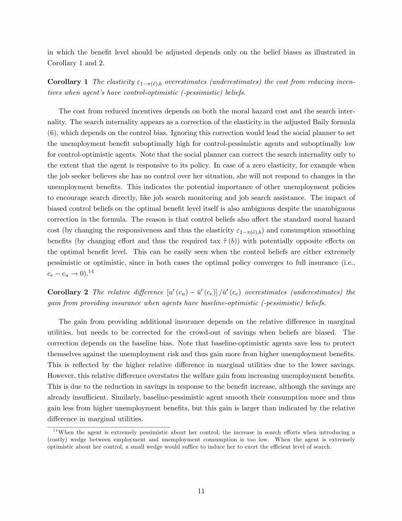
that consumption is independent of the length of unemployment. The left panels of Figures C.1

and C.2 in appendix show the net unemployment subsidy b+ τ −∆ψ for different belief parameters

with ∆ψ = ψu (e)−ψe. Given that the costs of effort are expressed in monetary terms, the subsidyis presented net of these costs. In the absence of savings, the static wedge between the marginal

utility of consumption when employed and unemployed is determined by the wage minus this net

subsidy, w − [b+ τ −∆ψ]. I scaled the wage to 1 such that the results can be interpreted in

percentage terms relative to output. The right panels show the monthly exit probability out of

unemployment. Both baseline-optimistic beliefs and control-pessimistic beliefs increase the cost of

providing incentives and thus reduce the exit rate implied by the optimal policy. The monthly exit

probability decreases from .20 to .18 for the range of baseline beliefs and increases from .14 to .21

for the range of control beliefs. As discussed before, the impact of biased beliefs on the optimal

policy itself is ambiguous and, in the absence of savings, the beliefs only affect the search effort.

For different values of the baseline beliefs, the optimal unemployment subsidy remains around .88,

implying a static wedge of around .12. The changes are more pronounced for different control beliefs.

In particular, the unemployment subsidy increases to 1 when the control beliefs become extremely

pessimistic. The static wedge disappears as providing incentives becomes useless. As discussed in

Section 3.3, private insurers would accommodate the job seekers’changing perception of the value

of insurance and thus lower the unemployment subsidy when the job seekers are baseline-optimistic.

I calculate the unemployment subsidy that they would provide in a competitive equilibrium as a

natural benchmark for the unemployment policy.22 When the optimistic baseline bias increases

to 200%, the net unemployment subsidy decreases to about 0.5. This approximately equals the

cost differential −∆ψ implying that the underlying unemployment benefit level is close to 0. At

200%, the baseline bias makes it unprofitable for private insurers to provide positive unemployment

benefits in this model.23

Optimal Dynamic Policy (With Savings). I now consider the optimal ‘dynamic’policy.

That is, the optimal constant policy (b, τ) when the agent has free access to a riskless asset such

that the agent’s consumption decreases linearly with the length of the unemployment spell at rate

rx. The left panel in Figure C.3 contrasts this dynamic wedge with the static wedge which is now

22The characterization of the competitive equilibrium discussed in section 3.3 and derived in the web appendixnaturally generalizes for the dynamic model.23The lower subsidy relative to the optimal policy induces more search as well. The monthly exit rates are up to

2 percentage points larger than in the social optimum.

19

reduced by x (i.e., w − [b+ τ −∆ψ]− x). Both wedges are evaluated given the optimal policy fordifferent baseline beliefs. The first thing to notice is that the optimal static wedge falls below .01

when the job seeker has access to savings (from about .12 in the absence of savings). The assets

allow using all future periods in this infinite-horizon model to smooth the loss of income during

unemployment. With unbiased beliefs, the static wedge equals .009 for the optimal policy, while the

dynamic wedge equals just above .002. This dynamic wedge increases substantially when the agent

underestimates how long she will remain unemployed. For a baseline bias of 200%, the dynamic

wedge has increased above .004 while the static wedge has decreased to below .007. In other words,

while the consumption of someone who finds work immediately is hardly 1% higher than the net

consumption of an unemployed job seeker at the start of spell, this difference increases by almost 1%

for any additional two months in unemployment. A job seeker who finds work only after two years

consumes almost 10% less (in each remaining period of her infinite life). The right panel shows the

unemployment subsidy b + τ − ∆ψ and the asset depletion x underlying the static and dynamic

wedge. The optimal policy involves a lower unemployment subsidy for baseline-optimistic agents,

but the static wedge between employment and unemployment consumption is still smaller since the

baseline-optimistic agent uses more of her assets to increase her unemployment consumption. I also

calculate the optimal policy when the social planner can directly control savings and thus effectively

determine the (linear) rate at which consumption decreases with the length of unemployment as in

Proposition 3. Surprisingly, this rate is hardly different, even for optimistic baseline beliefs, which

indicates that the static unemployment subsidy adjusts to induce a similar dynamic wedge.24

Welfare. Figure C.4 compares the welfare impact of the above policies by showing compen-

sating variations that make an unemployed job seeker without the policy as well of as with the

policy. The compensating variation is expressed as the present value of a constant consumption

flow, which is between one and two months worth of output in this numerical exercise. Providing

access to savings (i.e., switching from a static to a dynamic unemployment policy) substantially

increases the value of the unemployment policy as this allows to spread the unemployment risk

over all future periods. The value-added hardly depends on whether the access to savings can

be controlled or not. The adjustment of the unemployment subsidy to induce the unemployed to

deplete their savings at a desirable rate thus comes at a small cost, even when they are optimistic

about the duration of their unemployment spell. As a consequence, the value of the optimal policy

is fairly constant for different baseline beliefs. Note that the dynamic model allows biased beliefs

to distort the agent’s behavior only during the unemployment spell. In a more general model,

baseline beliefs would also affect the agent’s willingness to protect against unemployment through

precautionary savings (or other self-insurance). The welfare of the policy provided in a competitive

equilibrium illustrates the potential magnitude of these effects within this dynamic model. Private

insurers cater to the low value baseline-optimistic workers attach to unemployment protection by

24As discussed before, a baseline-optimistic agent may choose a higher depletion rate for a given unemploymentsubsidy than is socially optimal. In this case of unobservable savings, the simulation finds a lower subsidy, but asimilar depletion rate. This indicates the importance of the positive incentive effect of faster depletion during theunemployment spell, which the agent does not account for.

20

reducing the unemployment subsidy. Figure C.4 shows that the welfare of this policy is in fact

strongly decreasing in the baseline-optimistic bias and reaches zero for a bias of 200%.

6 Conclusion

This paper argues that perceptions of employment prospects should be at the heart of the design

of unemployment policies. New evidence reveals a striking optimistic bias suggesting that workers

underestimate the unemployment risk and the risk of long unemployment spells in particular.

Optimistic workers invest too little to protect themselves against the loss of earnings. Optimistic job

seekers do too little to leave unemployment and will be unprepared for long unemployment spells.

A natural way to reduce the negative impact of optimistic beliefs is to provide better information.

Information policies have been successful in other areas (e.g. health risks), but may be challenging

in the context of unemployment. As long as the bias persists, the analysis in this paper shows that

the use of future incentives (e.g., time limits on unemployment benefits) is particularly ineffective in

encouraging displaced workers to search harder or accept job offers earlier on. Moreover, empirical

estimates of standard behavioral responses like the policy elasticity of unemployment become an

inaccurate guide for policy design since they get a different interpretation when affected by biased

beliefs. This insight naturally extends to the design of other government policies based on so-called

"suffi cient statistics". More generally, policy makers should be cautious when relying on individuals’

actions to avoid risks or to protect themselves against their consequences. The strong optimistic

bias suggests that the use of private savings accounts or the reliance on the private provision of

insurance would be problematic. Competition would discipline private insurers to charge actuarially

fair prices, but not to correct the agents’ distorted choices. In fact, the low perceived value of

unemployment protection may help explain the puzzle why unemployment insurance is publicly

provided in almost all countries (Acemoglu and Shimer 2000).

The analysis highlights the importance of the control beliefs next to the beliefs about the

baseline risk. The empirical evidence on control beliefs is lagging and credible identification seems

particularly challenging. The experimental evidence on the illusion of control (see Langer 1975)

would suggest that job seekers are optimistic about the returns to their search efforts, but the many

unemployed who are not currently looking for employment because they are discouraged over job

prospects may well be underestimating these returns. For the job seekers in the study by Price et

al. (1998), I find that those who report to search more frequently expect shorter unemployment

spells, but the reduction in the experienced unemployment spells is even larger. This result could

indicate that job seekers are control-pessimistic next to being baseline-optimistic. Both biases slow

down the exit out of unemployment and contribute to its persistence. Further research should

shed more light on this and investigate the role of job seekers’perceptions for other unemployment

features. For example, the high incidence of long-term unemployment, in particular during the

Great Recession (Kroft et al., 2013), could be the result of beliefs adjusting slowly to deteriorating

employment prospects during the unemployment spell and during recessions.

21

Appendix A: Proofs

Proof of Proposition 1The social planner solves

maxbu(w − τ (b)− s (b))+

β [π (e (b))u (w − τ (b) + (1 + r) s (b)) + (1−π (e (b)))u(b+ (1 + r) s (b))− e (b)] ,

where τ (b) , s (b) and e (b) are implicitly defined by the incentive compatibility constraints ICe, ICsand the budget constraint BC. The implicit functions are assumed to be well-behaved such that

the optimal benefit level is characterized by the first-order condition

dU

db= 0⇔ ∂U

∂b+∂U

∂ττ ′ (b) +

∂U

∂ee′ (b) +

∂U

∂ss′ (b) = 0, with

∂U

∂b= β (1− π (e))u′(cu),

∂U

∂τ= −u′(c0)− βπ (e)u′ (ce) ≡ − (1 + βπ (e)) u′ (ce) ,

τ ′ (b) =1

1+r (1− π (e))

1 + 11+rπ (e)

[1 + ε1−π(e),b

],∂U

∂e= −β

[π′ (e)− π′ (e)

][u(ce)− u(cu)] and

∂U

∂s= β (1 + r) [π (e)− π (e)]

[u′(cu)− u′(ce)

],

where the last two expressions use ICe and ICs respectively. For ε1−π(e),b = −π′ (e) be′ (b) / [1− π (e)]

and β (1 + r) = 1, we find

dU

db/β (1− π (e)) = u′(cu)− u′ (ce)

[1 + ε1−π(e),b

]+π′ (e)− π′ (e)

π′ (e)

u(ce)− u(cu)

bε1−π(e),b

+π (e)− π (e)

β (1− π (e))

[u′(cu)− u′(ce)

]s′ (b) = 0⇔

u′(cu)− u′ (ce)u′ (ce)

[1− π (e)− π (e)

1− π (e)

1

β

u′(cu)− u′(ce)u′(cu)− u′ (ce)

(−s′ (b)

)]= ε1−π(e),b

[1− π′ (e)− π′ (e)

π′ (e)

u(ce)− u(cu)

bu′ (ce)

].

The adjusted Baily formula (6) for the social optimum directly follows from this expression.�

Proof of Lemma 1Denote the perceived expected utility of unemployed agent with assets a for an unemployment

policy z by U (z|a). The assets are used by an agent with CARA preferences to increase consumption

in all states by the same amount r1+ra. For CARA utility, we have u (x+ y) = u (x) exp (σy) and

u′ (x+ y) = u′ (x) exp (σy). The marginal utilities determining the agent’s optimal consumption

22

allocation and effort choice are thus all rescaled by the same amount exp (σr/ (1 + r) a).

Facing a constant policy z = (b, τ), an employed agent with assets a and CARA preferences

consumes her after-tax wage plus the interest on her asset level, ce (a) = r/ (1 + r) a + w − τ . Idenote her consumption level when unemployed by cu (a) = r/ (1 + r) a+ b+ x. When consuming

x more than her current income, her asset level decreases to a− (1 + r)x by the next period. This

decreases all her future consumption levels by rx. Her perceived expected utility when unemployed

can be written recursively with her assets a as the single state variable,

U (b, τ |a) = maxe,x

u (cu (a)− e) + βπ (e)u (ce (a)− rx)

1− β + β (1− π (e)) U (b, τ |a− (1 + r)x) .

Using the property of CARA preferences, this can be rewritten as U (b, τ |a) = exp (σr/ (1 + r) a) U (b, τ |0).

Hence, the agent’s problem is stationary and she chooses the same effort e and increase in con-

sumption x throughout the unemployment spell. From the recursive formulation, it then follows

that

U (b, τ |0) =u (b+ x− e) + βπ (e) u(w−τ−rx)

1−β

1− β (e, x),

with β (e, x) = β (1− π (e)) exp (σrx).�

Proof of Proposition 2The social planner maximizes the agent’s true expected utility given the implicit functions τ (b) , e (b)

and x (b) defined by IC ′e, ICx and the budget constraint τ = rb/π (e). That is

maxb

u(

r1+ra+ b+ x (b)− e (b)

)+ β

1−βπ (e (b))u(

r1+ra+ (w − τ (b))− rx (b)

)1− β (e (b) , x (b))

.

with β (e, x) = β (1− π (e)) exp (σrx). The first-order condition equals

∂U

∂b+∂U

∂ττ ′ (b) +

∂U

∂ee′ (b) +

∂U

∂xx′ (b) = 0, with

∂U

∂b+∂U

∂ττ ′ (b) =

[u′(cu − e)− u′(ce − rx)

(1 + ε1/π(e),b

)]/ [1− β (e, x)] , since

∂U

∂b= u′(cu − e)/ [1− β (e, x)] ,

∂U

∂τ= − β

1− βπ (e)u′(ce − rx)/ [1− β (e, x)] and

τ ′ (b) =r

π (e)

[1 + ε1/π(e),b

], and with,

∂U

∂e= −

{1− π′ (e)

π′ (e)

1− β (e, x)

1− β (e, x)

}u′ (cu − e)1− β (e, x)

, (12)

∂U

∂x= − [π (e)− π (e)]

exp (σrx) [u′ (cu − e)− u′ (ce)][1− β (e, x)]2

, (13)

23

using IC ′e and ICx for the last two expressions. Using the above expressions in the FOC with

ε1/π(e),b = π′ (e) be′ (b) /π (e) and [u′ (cu − e)− u′ (ce)] / [u′(cu − e)− u′(ce − rx)] = [exp (σrx) (1− π (e))]−1

from ICx, I find

dU

db= 0⇔ u′(cu − e)− u′(ce − rx)

u′(ce − rx)

[1 +

π (e)− π (e)

1− π (e)

(−x′ (b))1− β (e, x)

]= ε1/π(e),b

[1−

{1− π′ (e)

π′ (e)

1− β (e, x)

1− β (e, x)

}u′ (cu − e)u′(ce)b

π (e)

π′ (e)

].

The adjusted Baily formula for the constant policy immediately follows. Note that for

Q (b) =

(−π′′ (e)rσπ′ (e)

− 1

)(r +

u′ (ce)

u′ (cu − e)π (e) exp (σrx)

)u′ (cu − e)− u′ (ce)

u′ (ce)− exp (σrx) τ

π′ (e)

π (e),

total differentiation of the agent’s FOC’s (IC ′e and ICx) yields

e′ (b) = −exp (σrx)

Q (b)and x′ (b) = −

(exp (σrx)− 1)(−π′′(e)rσπ′(e)

− 1)

+ exp (σrx)

Q (b).

Hence, since e′ (b) < 0 for the optimal benefit level, Q (b) > 0. This implies that−π′′ (e) /[rσπ′ (e)

]−

1 > 0 from the above expression for Q (b). Hence, x′ (b) < 0.�

Proof of Proposition 3When the social planner can set x at zero cost, he maximizes the agent’s true expected utility

with respect to (b, τ , x) such that IC ′e and the budget constraint τ = rb/π (e) are satisfied. At the

optimum, a budget-balanced increase in x cannot increase the agent’s welfare. Consider the case

where b is adjusted to keep the budget balanced. That is, IC ′e and the budget constraint implicitly

define e (x) and b (x) when keeping τ fixed. Hence,

dU

dx= 0⇔ ∂U

∂x+∂U

∂bb′ (x) +

∂U

∂ee′ (x) = 0, with

∂U

∂x=

π (e) exp (σrx)u′ (cu − e)[1− β (e, x)]2

[u′ (cu − e)− u′ (ce)

u′ (cu − e)− 1

π (e)

(1− 1

exp (σrx)

)],

∂U

∂b=

u′ (cu − e)1− β (e, x)

and∂U

∂e= −

{1− π′ (e)

π′ (e)

1− β (e, x)

1− β (e, x)

}u′ (cu − e)1− β (e, x)

.

From total differentiation of the incentive compatibility and budget constraint defining the implicit

functions, I find

b′ (x) =π′ (e)

π (e)be′ (x) and e′ (x) =

r + u′(ce−rx)u′(cu−e)

π′(e)σr (exp(σrx)− 1)(

−π′′(e)σπ′(e)

+ 1)(

1− β (e, x)) ,

24

implying e′ (x) > 0 and b′ (x) > 0. Using the expression for b′ (x) and ε1/π(e),x = π′ (e)xe′ (x) /π (e),

dU

dx= 0⇔

[u′ (cu − e)− u′ (ce)

u′ (cu − e)− 1

π (e)

(1− 1

exp (σrx)

)]+

[b−

{1− π′ (e)

π′ (e)

1− β (e, x)

1− β (e, x)

}π (e)

π′ (e)

]1− β (e, x)

π (e)x exp (σrx)ε1/π(e),x = 0.

The characterization of the optimal dynamic policy immediately follows.�

Proof of Proposition 4I use subindex 0 to denote the variables values in the first period of the unemployment spell and

subindex 1 to denote the variable values in all subsequent periods. The agent’s perceived expected

utility can be written recursively as

U (b, τ) = maxx0,e0

u

(r

1 + ra+ b0 + x0 − e0

)

+ βπ (e0)

u(

r1+ra+ w − τ0 − rx0

)1− β + (1− π (e0)) exp (σrx0) U (b1, τ1)

The lower the agent perceives her expected utility when still unemployed in the next period

U (b1, τ1), the lower her effort e0 and the higher her depletion x0 in the first period of unem-

ployment, i.e., ∂e0/∂U1 < 0, ∂x0/∂U1 > 0. With CARA preferences, her behavior in the first

period does not affect her future behavior.

Now start from the optimal constant policy (b, τ) and consider a budget-balanced increase in

b and τ like in Proposition 2, but only implemented after the first period of unemployment. The

impact on the agent’s true expected utility equals

dU

db1=

[[∂U

∂e0+∂U

∂P

∂P

∂e0

]∂e0

∂U1

+∂U

∂x0

∂x0

∂U1

]︸ ︷︷ ︸

≡A

dU1

db1+ β (1− π (e0))

dU1

db1, (14)

where U1 and U1 denote the true and perceived unemployment continuation values after the first

period of unemployment. Starting from the optimal contract, the budget-balanced increase in b1after the first period of unemployment has only a second-order impact on the true continuation

value by Proposition 2, i.e., dU1/db1 = 0. Hence, the second of the two terms in (14) equals zero.

The agent’s change in behavior at the start of the spell, however, affects both her true expected

utility U and the social planner’s budget P . If the agent is baseline-optimistic, increasing e and

decreasing x in every period would increase her true expected utility by (12) and (13) respectively

and therefore also when changing behavior only in the first period, so that ∂U/∂e0 > 0, ∂U/∂x0 < 0.

The increase in e0 also improves the planner’s budget, which can be used to increase the agent’s

welfare. Hence, the term A, the first of the two terms in (14), is positive if dU1/db1 < 0. I now

25

show that dU1/db1 < 0 if dU1/db1 = 0 for a baseline optimistic agent if in an optimal policy with

constant benefits

1 + π(e)−π(e)

1−β(e,x)

u′(cu−e)−u′(ce)u′(cu−e)

(−π′′(e)rσπ′(e)

(exp (σrx)− 1) + 1)≥ 1−β(e,x)

1−β(e,x)π′(e)π′(e)

. (15)

That is, at the optimal policy,

dU1

db1=∂U1

∂b1+∂U1

∂τ1τ ′1 (b1)︸ ︷︷ ︸

≡B

+∂U1

∂e1e′1 (b1) +

∂U1

∂x1x′1 (b1)︸ ︷︷ ︸

≡C

= 0, with

B =u′(cu − e)− u′(ce − rx)

[1 + ε1/π(e),b

]1− β (e, x)

,

C =u′(cu − e)1− β (e, x)

exp (σrx)

Q (b)

(1− 1−β(e,x)

1−β(e,x)π′(e)π′(e)

)+

π(e)−π(e)

1−β(e,x)

u′(cu−e)−u′(ce)u′(cu−e) exp (σrx)

(exp(σrx)−1

exp(σrx)

(−π′′(e)rσπ′(e)

− 1)

+ 1) .

Evaluated at the same policy,

dU1

db1=∂U1

∂b1+∂U1

∂τ1τ ′1 (b1) = B − π (e)− π (e)

π (e)

u′(ce − rx)[1 + ε1/π(e),b

]1− β (e, x)

Since B + C = 0, B < 0 if C > 0. For a baseline-optimistic agent, B < 0 implies dU1/db1 < 0 and

thus dU1/db1 = AdU1/db1 < 0. Now I establish when C > 0. As argued in the proof of Proposition

2, e′ (b) < 0 implies Q (b) > 0 and −π′′ (e) /[rσπ′ (e)

]− 1 > 0. Hence, C > 0 if condition (15) is

satisfied. Since the second term in the left-hand side of (15) is positive, there exists a positive upper

bound ζ such that (1 − β (e, x))π′ (e) /[(1− β (e, x)) π′ (e)

]≤ 1 + ζ is suffi cient for the condition

to be satisfied. Hence, it is suffi cient for the search internality to be small relative to the baseline

bias.�

Appendix B: Empirical Analysis and Calibration

Price et al. (1998) organized a survey to study the prevention of depression in couples facing job loss.

The study was conducted in and around two major urban areas in Michigan and Maryland from

1996 to 1998. All participants were recruited through state unemployment offi ces. Initial screening

retained 1, 487 job seekers, who were part of a couple. All retained subjects were unemployed for less

than 15 weeks and looking for work, but did not expect to be recalled to their former job. About

one month after the initial screening, the retained subjects and their partners were interviewed

for the first time. Two follow-up interviews were organized about six months and twelve months

later. A third follow-up interview was organized one month after the first interview, but only for

a subsample of the initial group. In Table B.1, I show sample averages of the demographics of the

retained job seekers. On average, the subjects have been unemployed for 6.9 weeks at the time of

26

the first interview.

B.1 Baseline Beliefs: Actual and Expected Duration

Figure B.1: Empirical cumulative distribution: actual

duration vs. expected duration of remaining unemployment

spell

The subjects are asked about their baseline expectations in the question: “How many weeks do

you estimate it will actually be before you will be working more than 20 hours a week?”I interpret

the subjects’ answers as the number of weeks they expect to remain unemployed. In follow-up

interviews, subjects are asked when they actually started working. 86% of the subjects found work

for more than 20 hours a week before the last interview, about one year after the first interview.

I compute the minimum duration of an unemployment spell, assuming that the other 14% of the

subjects found work on the date of the last interview. The average minimum duration equals 23.0

weeks, again starting from the first interview.25 The distribution of the differences between the

actual and expected number of weeks of unemployment is shown in Figure 1 in the Introduction.

The difference between the minimum actual duration and the expected duration is shown in dark

grey for the job seekers who have not found work before the last interview. The optimistic bias

in baseline beliefs also appears clearly in Figure B.1, comparing the empirical distributions of

the expected and actual unemployment durations. The cumulative distribution of the expected

25The average optimistic bias for the sample of job seekers for whom the expectations and the actual duration areknown (n = 1, 088) equals 15.3 weeks. This excludes subjects who report to works less than 20 hours at the startof the new job (n = 117) subjects. Including these subjects with the date they started this part-time job decreasesaverage optimism by less than a week. This also excludes subjects who report they have found a different job beforethe one they are currenly working on, but for which no start date is known (n = 89). Including these subjects withthe date they started their current job increases average optimism by 1.5 weeks. Including these subjects assumingthey immediately found a job decreases average optimism by 1.5 weeks.

27

duration stochastically dominates the cumulative distribution of the minimum duration.26 For any

number of weeks, the number of job seekers who expect their unemployment spell will end within

that time span exceeds the number of job seekers for whom the unemployment spell actually ends

within that time span.

In the web-appendix to this paper I discuss how selection effects and alternative interpretations

of the survey question are unlikely to explain this extreme optimistic bias. I also provide preliminary

evidence suggesting that the bias survives during the unemployment spell.

B.2 Control Beliefs: Relation between Effort and Duration

Subjects are also asked how frequently they have searched for work during the month before the

interview. The questions ask about reading the newspaper for job opportunities, checking with

employment agencies, checking with friends, sending out resumes, etc. I aggregate the answers to

these questions, giving each answer the same weight, and I estimate the impact of this search index

on the actual and expected duration of unemployment.27 ,28 The regressions of interest are

actual durationi = β1 searchi +Xiγ1 + εi, (16a)

expected durationi = β2 searchi +Xiγ2 + νi, (16b)

act. durationi - exp. durationi = (β1 − β2) searchi +Xi (γ1 − γ2) + εi − vi (16c)

with the durations starting from the first interview.

Table B.2 reports the ordinary least squares estimates for these three regressions. Unemploy-

ment spells are actually shorter for unemployed workers who report to search more intensively and

they also expect their spells to be shorter. The first effect is stronger than the second effect. If the

search index increases by one unit, which corresponds to doubling the frequency in every search

dimension, the actual unemployment spell is 3.4 weeks shorter, but the expected unemployment

spell is only 2.0 weeks shorter. Higher search levels correspond to lower optimism about the dura-

tion of unemployment. While the coeffi cients of search are significant at the 1% level in regressions

(16a) and (16b), the estimate of the difference in regression (16c) is only significant at the 10% level

(p -value = .08). If both effects were causal, the estimated average control bias would be −67%.

This is much less pronounced and significant than the baseline bias. Unobserved heterogeneity

26The kink in the cumulative distribution of the actual duration is due to the fact that I include the minimumduration for the job seekers with incomplete spells. These minimum durations are bunched around 52 weeks, whichis the average time between the first and the last interview.27The correlation between this search index and any of its nine components varies between 0.48 and 0.70. The

partner of each subject is asked the exact same questions about the subject’s efforts. The correlation between thesearch index as reported by the job seekers and their partners is 0.57.28The nine questions are: “During the past month, how often have you; read the newspaper and other publications

for job opportunities? checked with employment agencies? talked to friends, family, or other people you know to getinformation about jobs? used, or sent out a resume? filled out application forms for a job? telephoned, written orvisited potential employers? done things to improve the impression you would make in a job interview? contacteda public employment service? went out on information interviews?”The answer options are; 1. Not at all, 2. Onceevery 3 to 4 weeks, 3. Once every couple of weeks, 4. Every week, 5. Two or three times a week, 6. Every day.

28

affecting both the bias in beliefs and the search efforts or the reverse impact of beliefs on search

effort would bias the estimate of the control bias. The estimates are similar when using candidate

instrumental variables, including alternative measures of search, controlling for the willingness to

work or accounting for censoring and truncation issues, as discussed in an earlier version of this

paper (see Spinnewijn 2008).

B.3 Calibration of the Dynamic Model of the Unemployment Spell

The unit of time for the calibration is one month. The monthly discount factor equals β = 0.9956,

which corresponds to a yearly discount factor equal to 0.95. I assume that the monthly output

equals 1 when employed and 0 when unemployed. Given this rescaling, the CARA coeffi cient is set

equal to σ = 2.

Probability of Finding Work. I assume that effort e is linear in the number of times a jobseeker reports to have engaged in any of the search activities as discussed in the previous section.

I rescale this effort variable such that e = 0 corresponds to not having searched in any dimension

during the entire month and e = 1 corresponds to having searched every day in every dimension,

averaged over the entire month. In this interpretation, e = 0.15 corresponds to the sample average

of search effort (i.e. search in all dimensions between ‘once every couple of weeks’ and ‘every

week’). For these three values of search effort, the probability function π (e) = π0 +π1× e0.662 with

π0 = 0.140 and π1 = 0.170 approximates the average duration of unemployment, estimated using

ordinary least squares (Table B.2). I assume that the perceived monthly probability of finding work

as a function of effort equals π (e) = π0 + π1 × e0.662 and show how the optimal policy changes for

different values of π0 and π1 respectively.

Monetary Cost of Effort. I finally calibrate the monetary cost of search function ψu (e) =

ψ0eψ1 ,assuming that the monetary cost of effort when employed equals the monetary cost of search-

ing daily in every dimension ψe = ψ (1) = ψ0. I set ψ0 = 0.483 and ψ1 = 2.65 in order to match

the empirical exit rate and unemployment duration elasticity. In the US, unemployed workers are

eligible for unemployment benefits for six months. The mean and median replacement rate for

which the unemployed workers are eligible equal respectively 0.43 and 0.48. When implementing

a contract that pays b = 0.45 in the first six months and b = 0 afterwards, the calibrated model

predicts an average monthly probability of finding work equal to 0.19. This equals the average

monthly exit rate in the sample. Moreover, the predicted elasticity of unemployment duration with

respect to a constant benefit level b = 0.45 equals −.5. This corresponds to the empirical estimatesreviewed in Krueger and Meyer (2002). For the calibration of the cost function, I set the belief

parameters equal to π0 = 0.361 and π1 = 0.056, which implies an optimistic relative baseline bias

[π (e)− π (e)] /π (e) equal to 100% (at the average effort level e = 0.15), which is more modest

than the average baseline bias in the sample of about 200%, and a pessimistic relative control bias[π′ (e)− π′ (e)

]/π′ (e) equal to −67%, which corresponds to the relative ratio of the least squares

estimates of the actual and perceived impact of search (Table B.2).

29

Table B.1Summary Statistics

Obs. Mean StDev Obs. Mean StDev

Male 1,339 .55 .50 Partner’s education 1,137 13.50 2.20

Age 1,339 38.48 9.96 Monthly wage2 1,320 2.60 1.72

White 1,339 .67 .47 Times unemployed 1,339 .34 .47

Married 1,339 .81 .39 Weeks displaced3 1,339 6.91 4.16

Children 1,339 1.30 1.25 Search (at 1st int.) 1,249 3.34 .87

Education1 1,334 13.63 2.14 Search (at 3rd int.) 1,249 3.35 .95

Maryland 1,339 .45 .50 Actual duration4 1,223 23.04 21.03

Partner empl. 1,139 .79 .41 Expected duration 1,182 6.83 8.601 Expressed in number of years. 2 Earned on the last job before unemployment, expressed in 1000 USD. 3 Since thestart of the current unemployment spell. 4 Includes censored spells with the duration between thefirst and last interview.

Table B.2OLS Estimates of the Effect of Search and Covariates on the Actual Duration of Unemployment (1), the

Expected Duration of Unemployment (2) and the Difference Between the Actual and the Expected

Duration of Unemployment (3)

Actual duration Expected duration Optimism

(1) (2) (3)

Search -3.30 [757]∗∗ -2.03 [.369]∗∗ -1.36 [.780]

Male -3.45 [1.34]∗ -1.88 [.457]∗∗ -1.58 [1.39]

Age .201 [.073]∗∗ .048 [.021]∗ .153 [.072]∗

White -5.82 [1.50]∗∗ -.544 [.596] -5.28 [1.54]∗∗

Married -5.07 [1.89]∗∗ .306 [.576] -5.37 [1.89]∗∗

Children .783 [.528] .410 [.274] .373 [.544]

Education -.343 [.368] .317 [.126]∗ -.659 [.362]

Maryland -2.97 [1.35]∗ .124 [.493] -3.09 [1.34]∗

Partner employed -2.78 [1.62] .242 [.501] -3.02 [1.64]

Partner education .014 [.337] .205 [.115] -.192 [.333]

Monthly wage before unemp. -.732 [.392] .490 [.194]∗ -1.21 [.369]∗∗

Times unemployed -1.22 [1.35] -.294 [.453] -.925 [1.32]

Weeks since displacement .428 [.165]∗∗ .134 [.064]∗ .294 [.163]

Obs. 1,007 1,007 1,007

R2 .087 .115 .078

Robust standard errors are in parentheses. * denotes statistical significance at the 5% level, ** at the 1% level.

30

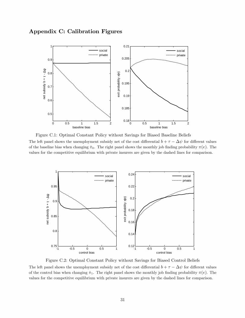
Appendix C: Calibration Figures

0 0.5 1 1.5 2

0.5

0.6

0.7

0.8

0.9

1

baseline bias

net s

ubsi

dy b

 +τ 

­ ∆ψ

0 0.5 1 1.5 20.18

0.185

0.19

0.195

0.2

0.205

0.21

baseline bias

exit 

prob

abili

tyπ(

e)

socialprivate

socialprivate

Figure C.1: Optimal Constant Policy without Savings for Biased Baseline Beliefs

The left panel shows the unemployment subsidy net of the cost differential b+ τ −∆ψ for different valuesof the baseline bias when changing π0. The right panel shows the monthly job finding probability π(e). Thevalues for the competitive equilibrium with private insurers are given by the dashed lines for comparison.

­1 ­0.5 0 0.5 10.75

0.8

0.85

0.9

0.95

1

control bias

net s

ubsi

dy b

 +τ 

­ ∆ψ

­1 ­0.5 0 0.5 10.12

0.14

0.16

0.18

0.2

0.22

0.24

control bias

exit 

prob

abili

tyπ(

e)

socialprivate

socialprivate

Figure C.2: Optimal Constant Policy without Savings for Biased Control Beliefs

The left panel shows the unemployment subsidy net of the cost differential b+ τ −∆ψ for different valuesof the control bias when changing π1. The right panel shows the monthly job finding probability π(e). Thevalues for the competitive equilibrium with private insurers are given by the dashed lines for comparison.

31

0 0.5 1 1.5 22

3

4

5

6

7

8

9

10x 10­3

baseline bias

dyna

mic

 wed

ge r*

x  (f

ull)

stat

ic w

edge

 w ­

τ ­ b

 +∆

ψ (d

ash)

0 0.5 1 1.5 20

0.1

0.2

0.3

0.4

0.5

0.6

0.7

0.8

0.9

1

baseline biasde

plet

ion 

x (fu

ll)ne

t sub

sidy

 b +

τ ­ ∆

ψ (d

ash)

unobservable savingscontrolled savings

Figure C.3: Optimal Constant Policy with Savings for Biased Baseline BeliefsThe left panel shows the dynamic wedge rx (full line) and the static wedge w − τ − b+ ∆ψ (dashed line)implied by the optimal constant policy for different values of the baseline bias when changing π0. The rightpanel shows the underlying unemployment subsidy τ − b+ ∆ψ (dashed line) and depletion level x (fullline). In the right panel, values are also shown for the optimal policy with controlled savings for comparison.

0 0.2 0.4 0.6 0.8 1 1.2 1.4 1.6 1.8 2­0.5

0

0.5

1

1.5

2

baseline bias

com

pens

atin

g va

riatio

n

constant policy w/ unobservable savingsconstant policy w/ controlled savingsconstant policyprivate policy

Figure C.4: Welfare Comparison of Unemployment Policies for Biased Baseline BeliefsThe figure shows the compensating variation that make an unemployed job seeker without the policy as wellof as with the policy for four unemployment policies. The compensating variation is expressed as the presentvalue of a constant consumption flow. The four policies are the optimal unemployment policy without accessto savings, with unobservable savings, with controlled savings and the policy provided by private insurers ina competitive equilibrium.

32

References

Acemoglu, Daron, and Robert Shimer. 2000. “Productivity Gains from Unemployment Insur-

ance.”European Economic Review, 44: 1195-1224.

Altman, Daniel, and Martin S. Feldstein. 2006. “Unemployment Insurance Savings Accounts.”

In Tax Policy and the Economy, Volume 21, ed. James Poterba, 35-61. Cambridge: MIT Press.

Baily, Martin N. 1978. “Some Aspects of Optimal Unemployment Insurance.”Journal of Public

Economics, 10: 379-402.

Bénabou, Roland, and Jean Tirole. 2002. “Self-Confidence and Personal Motivation.”Quarterly

Journal of Economics, 117: 871-915.

Bénabou, Roland, and Jean Tirole. 2006. “Belief in a Just World and Redistributive Politics.”

Quarterly Journal of Economics, 121: 699-746.

Bernheim, B. Douglas, and Antonio Rangel. 2007. “Behavioral Public Economics: Welfare and

Policy Analysis with Non-standard Decision Makers.” In Economic Institutions and Behavioral

Economics, eds. Peter Diamond and Hannu Vartiainen, 7-77. Princeton: Princeton University

Press.

Brunnermeier, Markus K., and Jonathan A. Parker. 2005. “Optimal Expectations.”American

Economic Review, 95: 1092-1118.

Chetty, Raj. 2006. “A General Formula for the Optimal Level of Social Insurance.”Journal of

Public Economics, 90: 1879-1901.

Chetty, Raj. 2008. “Moral Hazard vs. Liquidity and Optimal Unemployment Insurance.”

Journal of Political Economy, 116: 173-234.

Chetty, Raj. 2009. “Suffi cient Statistics for Welfare Analysis: A Bridge Between Structural

and Reduced-Form Methods.”Annual Review in Economics, 1: 451-488.

Chetty, Raj, and Emmanuel Saez. 2010. “Optimal Taxation and Social Insurance with En-

dogenous Private Insurance.”American Economic Journal: Economic Policy, 2: 85-114.

Compte, Olivier, and Andrew Postlewaite. 2004. “Confidence-Enhanced Performance.”Amer-

ican Economic Review, 94: 1536-1557.

Cutler, David, and Richard Zeckhauser. 2004. “Extending the Theory to Meet the Practice of

Insurance.”In: Litan, R., and Herring, R. (Eds), Brookings-Wharton Papers on Financial Services.

Washington: Brookings Institution.

De Bondt, Werner and Richard Thaler. 1995. “Financial Decision-making in Markets and

Firms: a Behavioral Perspective,”in Handbooks in Operations Research and Management Science,

eds. R. A. Jarrow, V. Maksimovic, and W. T. Ziemba, 385—410. North Holland.

de la Rosa, Leonidas. 2011. “Overconfidence and Moral Hazard.”Games and Economic Be-

havior, 73: 429—451.

DellaVigna, Stefano. 2009 “Psychology and Economics: Evidence from the Field.”Journal of

Economic Literature, 47: 315-372.

DellaVigna, Stefano, and M. Daniele Paserman. 2005. “Job Search and Impatience.”Journal

of Labor Economics, 23: 527-588.

33

Eliaz, Kfir, and Ran Spiegler. 2008. “Consumer Optimism and Price Discrimination.”Theo-

retical Economics, 3: 459-497.

Ellison, G., 2006. Bounded Rationality in Industrial Organization. In: Blundell, R., Newey,

W., and Persson, T. (Eds.), Advances in Economics and Econometrics: Theory and Applications,

Ninth World Congress, 142-174. Cambridge: Cambridge University Press.

Gervais, Simon and Terrance Odean. 2001. “Learning to be Overconfident.”Review of Financial

Studies, 14: 1-27.

Gollier, Christian. 2005. “Optimal Illusions and Decisions under Risk.”CESifo Working Paper

1382.

Grubb, Michael D. 2010. “Selling to Overconfident Consumers.”American Economic Review,

99: 1770-1807.

Gruber, Jonathan. 1997. “The Consumption Smoothing Benefits of Unemployment Insurance.”

American Economic Review, 87: 192—205.

Hopenhayn, Hugo A., and Juan Pablo Nicolini. 1997. “Optimal Unemployment Insurance.”

Journal of Political Economy, 105: 412-438.

Kanbur, Ravi, Jukka Pirttila, and Matti Tuomala. 2006. “Non-Welfarist Optimal Taxation and

Behavioural Public Economics.”Journal of Economic Surveys, 20: 849—868.

Kroft, Kori, Fabian Lange, Matthew Notowidigdo and Larry Katz. 2013. “Long-Term Unem-

ployment and the Great Recession: The Role of Composition, Duration Dependence, and Non-

Participation.”Harvard working paper.

Köszegi, Botond. 2006. “Ego Utility, Overconfidence, and Task Choice.”Journal of the Euro-

pean Economic Association, 4: 673—707.

Köszegi, Botond, and Matthew Rabin. 2007. “Mistakes in Choice-Based Welfare Analysis.”

American Economic Review, 97: 477-481.

Köszegi, Botond, and Matthew Rabin. 2008. “Revealed Mistakes and Revealed Preferences.”In

The Foundations of Positive and Normative Economics, eds. Andrew Caplin and Andrew Schotter,

193-209. Oxford: Oxford University Press.

Krueger, Alan B., and Bruce D. Meyer. 2002. “Labor Supply Effects of Social Insurance.” In

Handbook of Public Economics, Volume 4, eds. Alan Auerbach and Martin Feldstein, 2327-2392.

Amsterdam: North-Holland.

Landais, Camille. 2013. “Assessing the Welfare Effects of Unemployment Benefits Using the

Regression Kink Design.”LSE working paper.

Langer, Ellen J. 1975. “The Illusion of Control.”Journal of Personality and Social Psychology,

32: 311-328.

Manski, Charles F. 2004. “Measuring Expectations,”Econometrica, 72(5): 1329-1376.

McCall, John. 1970. “Economics of Information and Job Search,”Quarterly Journal of Eco-

nomics, 84: 113—126.

Moore, Don A. and Paul J. Healy. 2008. “The Trouble With Overconfidence,”Psychological

Review, 115 (2): 502-517.

34

Mueller, Andreas and Johannes Spinnewijn. “Expectations about Employment Prospects dur-

ing the Unemployment Spell: Evidence from Longitudinal Data,”In progress.

Mullainathan, S., Schwartzstein, J., and W. Congdon, 2012. A Reduced Form Approach to

Behavioral Public Finance. Annual Review of Economics, 4: 511-540.

Paserman, M. Daniele. 2008. “Job Search and Hyperbolic Discounting: Structural Estimation

and Policy Evaluation,”Economic Journal, 118: 1418-1452.

Price, Richard H., Amiram D. Vinokur, George Howe, and Robert D. Caplan. 2004. Preventing

Depression in Couples facing Job Loss, 1996-1998: Baltimore, Maryland, and Detroit, Michigan.

Ann Arbor, MI: Institute for Social Research, Survey Research Center, and Michigan Prevention

Research Center/Washington, DC: George Washington University, Center for Family Research

[producers], 1998. Ann Arbor, MI: Inter-university Consortium for Political and Social Research

[distributor], 2004.

Sandroni, Alvaro, and Francesco Squintani. 2007. “Overconfidence, insurance and Paternal-

ism.”American Economic Review, 97: 1994-2004.

Santos-Pinto, Luis. 2008. “Positive Self-Image and Incentives in Organizations.” Economic

Journal, 118: 1315-1332.

Shavell, Steven, and Laurence Weiss. 1979. “The Optimal Payment of Unemployment Insurance

Benefits Over Time.”Journal of Political Economy, 87: 1347-1362.

Shimer, Robert, and Iván Werning. 2007. “Reservation Wages and Unemployment Insurance.”

Quarterly Journal of Economics, 122: 1145-1185.

Shimer, Robert, and Iván Werning. 2008. “Liquidity and Insurance for the Unemployed.”

American Economic Review, 98: 1922-1942.

Slovic, Paul. 2000. The Perception of Risk. London: Earthscan.

Spinnewijn, Johannes. 2008. “Unemployed, but Optimistic: Optimal Insurance Design with

Biased Beliefs.”Available at SSRN: http://ssrn.com/abstract=1291566.

Spinnewijn, Johannes. 2012. “Heterogeneity, Demand for Insurance and Adverse Selection.”

CEPR DP8833.

Spinnewijn, Johannes. 2013. “Insurance and Perceptions: How to Screen Optimists and Pes-

simists.”Economic Journal, 123: 606-633.

Tversky, Amos, and Daniel Kahneman. 1974. “Judgment under Uncertainty: Heuristics and

Biases.”Science, 185: 1124-1131.

Van den Steen, Eric J. 2004. “Rational Overoptimism (and Other Biases).”American Economic

Review, 94: 1141-1151.

Weinstein, Neil D. 1980. “Unrealistic Optimism about Future Life Events.”Journal of Person-

ality and Social Psychology, 39(5): 806-820.

Werning, Iván. 2002. “Optimal Unemployment Insurance with Unobservable Savings.”MIT

Working Paper.

35

7 Web Appendix to "Unemployed but Optimistic: Optimal In-

surance Design with Biased Beliefs"

This web appendix provides two pieces of complementary analysis. First, I discuss the robustness of

the optimistic bias presented in the introduction and appendix of the paper. Second, I characterize

the competitive equilibrium with profit-maximizing insurers discussed in Section 3.3.

7.1 Optimistic Bias

In this section I discuss how selection effects and alternative interpretations of the survey question

are unlikely to explain the bias in expectations. I also provide preliminary evidence suggesting that

the optimistic bias survives during the unemployment spell.

Selection Effects Selection effects seem to play a minor role in explaining the optimistic bias for

the sample considered in Price et al. (1998). First, the average unemployment duration decreases

in the US between 1996 and 1998, as did the average unemployment rates in four out of the

five counties considered in the sample. It seems unlikely that job seekers were surprised by an

unexpected deterioration of economic conditions. Second, by screening through state unemployment

offi ces, only job seekers who are filing for unemployment benefits are selected. These job seekers

are the most policy relevant group of unemployed workers. Moreover, this selection effect does not

necessarily increase the estimate of baseline optimism either. Anderson and Meyer (1997) document

that the main reason why displaced workers do not take up unemployment benefits is that they

expect that the unemployment spell will be short.29 Third, the sample characteristics are similar

to the characteristics of the unemployed in Maryland and Michigan between 1996 and 1998 in the

Current Population Survey.30 Fourth, the job seekers in this sample have been unemployed for 7

weeks on average at the time of the first interview. This implies that both job seekers with ex

post short unemployment spells and baseline-pessimistic job seekers, who search more intensively,

are likely to be underrepresented in the sample. However, the average baseline-optimistic bias is

hardly smaller for the newly unemployed. For the 249 job seekers who have been unemployed for

3 weeks or less, the average optimistic bias equals 14.5 weeks. The Wilcoxon rank-sum test does

not reject that the baseline bias has the same distribution for the recently displaced job seekers

and the other job seekers (p-value = .79). Fifth, exit rates tend to decrease with the duration of

unemployment, which may explain why the average remaining duration in the sample considered

here is high. The average duration of unemployment for newly unemployed is about 14 weeks in29Anderson and Meyer (1997) find that 37 percent of the job losers and leavers eligible for UI give ‘Expected to

get another job soon/be recalled’as the reason for not applying for UI, whereas no other single reason is given bymore than 7 percent of them.30Out of the 425 unemployed in Maryland and Michigan in the March CPS between 1996 and 1998, 54 percent are

male and 69 percent are white, compared to 53 percent and 73 percent respectively in the sample considered in thispaper. The unemployed in the CPS sample have less education and are younger. This may be explained by the factthat this sample is restricted to couples. Compared with the married unemployed in the CPS, the distributions ofeducation and age are more similar. Notice that baseline optimism is significantly higher for the less educated andnot significantly lower for the young job seekers.

36

Figure 2: Histogram of the reported expectations with bins labeled by the percentiles of the actual duration

the US in 1996 (Valletta 1998). This is still twice as long as the average expectation in the sample.

Finally, the US economy was expanding during the period that the survey was organized, which may

affect the baseline bias. When a crisis hits, the average unemployment duration increases. With

unemployment at the centre of attention during the crisis, expectations may adjust even more such

that the optimistic bias would be smaller or even reversed. However, Mueller and Spinnewijn (in

progress) find an optimistic baseline bias that is as extreme in magnitude based on a survey of job

seekers in New Jersey, conducted during the Great Recession.

Reported Expectations One may be concerned about the extent to which the duration pre-

dictions capture the job seekers’ expectations on which they act. First, the job seekers are not

explicitly incentivized to report their expectations truthfully. I do not observe actual behavior

either, like their savings for instance, to verify to what extent their behavior is explained by the

reported expectations. The expectations do however explain half as much variation in the actual

duration of the unemployment spells as all other demographic and employment variables together.31

Also, the growing literature on the measurement of expectations confirms the predictive value of

surveyed expectations for both actual outcomes and future behavior (Manski 2004). Second, I

interpret the job seekers’reported point predictions as their subjective means. However, some job

seekers may report different distributional features as their point predictions, like the median or

any other percentile.32 The Figure suggests that it is unlikely that these alternative interpretations

of the question play an important role in explaining the optimistic bias. It shows the distribution

of the reported expectations by the percentiles of the actual duration distribution. That is, for

each job seeker it shows the percentile he or she should have had in mind if his or her reported

point prediction were to be accurate ex post. This assumes that the population distribution is the

31The R2 for the first regression in Table B.2, which regresses the actual duration on all considered covariates,increases from .087 to .128 when including the expected duration as an explanatory variable. The R2 for regressingthe actual duration on only the expected duration equals .052.32Engelberg, Manski and Williams (2009) argue that the elicitation of probabilistic forecasts is therefore more

instructive. Notice hovever that the use of these point predictions about the duration of unemployment does avoidbunching issues that arise when eliciting probabilities.

37

true distribution that all job seekers are facing. The point predictions are centered around the

20th percentile of the actual duration distribution, and more than 90% of the predictions are below

the median (and thus below the mean). Finally, an alternative question in the survey asking for

a probabilistic forecast suggests similar optimism about the baseline probability of finding work,

although it does not allow quantifying the bias.

Changes in Beliefs In the dynamic model of the unemployment spell in Section 4, I have made

the simplifying assumption that the perceived probability of finding work is not affected by the

duration of unemployment. This contradicts learning by unemployed workers. However, the beliefs

reported by the job seekers suggest that not much learning is going on.

First, the number of times a job seeker has been unemployed in the last three years does not

significantly lower his or her optimism about the current unemployment spell (p -value = .48), as

shown in Table B.2 in the appendix to the paper. Second, the number of weeks a job seeker has

been unemployed in the current spell even tends to increase the optimistic bias (p -value = .07).

Both results are cross-sectional and do not necessarily rule out that the optimistic baseline bias

decreases when job seekers become more experienced. Job seekers who are less optimistic about

finding a job may search more and leave unemployment earlier. However, suffi cient learning would

overcome this selection effect. Finally, unsuccessful job seekers hardly increase their expectations

during unemployment. I find that the distribution of expectations held by job seekers about the

remaining number of weeks of unemployment is very stable throughout the unemployment spell.

The average of the expectations at the first interview is not significantly different from the average

of the expectations one month or six months later, comparing the same sample of job seekers. Only

the job seekers who are still unemployed at the time of the last interview, about twelve months

after the first interview, report expectations that are significantly higher than at the first interview.

Together these results suggest that if some learning about the bias is going on, it is very modest.33

7.2 Competitive Equilibrium with Profit-Maximizing Insurers

The analysis highlights the potential importance of the agent’s decision to protect herself against

unemployment for the design of social insurance. In the context of unemployment insurance, the

role of private insurance is limited in practice. The question whether government interventions are

needed depends in the first place on whether the equilibrium coverage provided by private insurers

would be socially optimal. This section addresses this question by characterizing the equilibrium

contract (bp, τp) offered by competing private insurers in the absence of any public provision,

which is a natural benchmark for the optimal policy. A well-known result in public economics

is that moral hazard, in contrast with adverse selection, does not raise the need for government

33Notice that if job seekers are uncertain about their ability to find a job at the start, a longer unemploymentspell should make them revise their beliefs about the remaining duration upward. The data suggests that they arerevising their beliefs upward, at least after twelve months, however they may not revise suffi ciently and become moreoptimistic compared to an unbiased job seeker who is Bayesian updating, the longer they are unemployed. This iswhat Falk, Huffman and Sunde (2006) find in a laboratory experiment.

38

intervention per se (e.g., Chetty and Saez 2010). Competing private insurers would offer the socially

optimal insurance contract. This is no longer true when the agent’s beliefs are biased. In order

to attract agents, private insurers offer contracts that maximize the agents’perceived rather than

true expected utility. Notice that the wedge between private and social insurance is not suffi cient

to justify government interventions. A policy maker is not necessarily paternalistic, but may care

about an agent’s perceived welfare as when for example he would try to gain the agent’s vote in

elections. If a policy maker only cares about the agent’s perceived welfare, he would implement the

exact same policy as the competing profit-maximizing insurers.34

With competition driving profits down to zero, the contract (bp, τp) offered in a competitive

equilibrium is characterized by

maxb,τ

u(c0) + β [π (e)u(ce) + (1− π (e))u(cu)− e)] (17)

subject to ICe, ICs and the balanced budget constraint

τ +1

1 + r[π (e) τ − (1− π (e)) b] = 0. (BC)

The single difference with the social planner’s problem is that the uncertain outcomes of the agent’s

search effort are weighted with the perceived probabilities π (e) and 1 − π (e) to calculate the

perceived expected utility. In equilibrium, a budget-balanced increase in the benefit level bp and

tax level τp has no first-order impact on the agent’s perceived expected utility,

dU

db= 0 ⇔ ∂U

∂b+∂U

∂ττ ′ (bp) = 0. (18)

The equilibrium condition (18) reveals two differences with the social optimum. First, the rate

at which the tax τp needs to be increased when increasing the benefit bp is exactly the same

as before and depends on the true probabilities. However, the perceived value of this budget-

balanced increase depends on the perceived probabilities. For example, baseline-optimistic agents

underestimate the insurance value relative to its cost. This induces private insurers to lower the

unemployment benefit relative to the social planner. Second, the behavioral responses to a policy

change have only a second-order impact on the agent’s perceived expected utility. In contrast with

the social planner, private insurers do not try to correct the agent’s distorted effort and savings

choice. For example, in the case of control-optimistic agents who exert too much effort given the

true returns, this would again induce private insurers to reduce the unemployment benefit relative to

the social planner. The following Proposition characterizes the competitive equilibrium in absence

of social insurance.

34See Salanié and Treich (2009) for an analysis comparing policies by a paternalistic and populist policy maker.

39

Proposition 5 The equilibrium contract offered by profit-maximizing insurers is characterized by

1−π(e)1−π(e)u

′(cu)− 1+βπ(e)1+βπ(e) u

′ (ce)

1+βπ(e)1+βπ(e) u

′ (ce)= ε1−π(e),b, (19)

for u′ (ce) ≡ u′(c0)+βπ(e)u′(ce)1+βπ(e) and β (1 + r) = 1.

Proof. The competitive equilibrium solves

maxbu(w − τ (b)− s (b))+

β [π (e (b))u(w − τ (b) + (1 + r) s (b)) + (1−π (e (b)))u(b+ (1 + r) s (b))− e (b)] ,

where τ (b) , s (b) and e (b) are implicitly defined by ICe, ICs and BC. The first-order condition of

the maximization equalsdU

db= 0⇔ ∂U

∂b+∂U

∂ττ ′ (b) = 0, with

∂U

∂b= β (1− π (e))u′(cu),

∂U

∂τ= −u′(c0)− βπ (e)u′ (ce) ≡ − (1 + βπ (e)) u′ (ce) and

τ ′ (b) =1

1+r (1− π (e))

1 + 11+rπ (e)

[1 + ε1−π(e),b

].

The first-order impact of effort and savings responses on the perceived expected utility equals zero

by ICe and ICs, i.e., ∂U/∂e = ∂U/∂s = 0. Using the above expressions and β (1 + r) = 1, I can

rewrite the FOC as

dU

db/β (1− π (e)) =

1− π (e)

1− π (e)u′(cu)− 1 + βπ (e)

1 + βπ (e)u′ (ce)

[1 + ε1−π(e),b

]= 0⇔

1−π(e)1−π(e)u

′(cu)− 1+βπ(e)1+βπ(e) u

′ (ce)

1+βπ(e)1+βπ(e) u

′ (ce)= ε1−π(e),b.

The adjusted Baily formula (19) for the competitive equilibrium immediately follows.

A comparison of Proposition 1 here and Proposition 1 in the main text confirms that biases in

baseline beliefs and control beliefs drive a wedge between the social optimum and the competitive

equilibrium. Interestingly, competition forces private insurers to charge the actuarially fair price

for insurance and thus subjects them to the same budget constraint as the social planner, but it

does not force them to sell the optimal amount of insurance.35 In particular, when agents are too

optimistic about the risk of unemployment, providing insurance becomes unprofitable for private35DellaVigna (2009) discusses similar findings when agents have irrational expectations about their self-control

problems or inattention. For instance, DellaVigna and Malmendier (2004) find that competing firms will distort theconsumption of naive individuals with self-control problems, pricing investment goods below and leisure goods abovemarginal cost. Still, competition will drive down the fixed contract fee.

40

insurers. As discussed in the main text, this suggests a natural explanation for the puzzle of why

unemployment insurance is mostly publicly provided.36,37 In fact, if possible, private insurers would

undo the undervalued social insurance by buying unemployment insurance from the agent. In order

to increase the insurance coverage, the social planner would have to intervene by subsidizing private

insurance provision or regulating the private market.

7.3 Additional References

Anderson, Patricia M., and Bruce D. Meyer. 1997. “Unemployment Insurance Takeup Rates

and the After-Tax Value of Benefits.”Quarterly Journal of Economics, 112(3): 913-937.

DellaVigna, Stefano, and Ulrike Malmendier. 2004. “Contract Design and Self-Control: Theory

and Evidence.”Quarterly Journal of Economics, 119(2): 353—402.

Engelberg, Joseph, Charles F. Manski, and Jared Williams. 2009. “Comparing the Point Pre-

dictions and Subjective Probability Distributions of Professional Forecasters.”Journal of Business

& Economic Statistics, 156: 146-158.

Falk, Armin, David Huffman, and Uwe Sunde. 2006. “Self-Confidence and Search.” IZA Dis-

cussion Paper 2525.

Parsons, Donald, Torben Tranaes and Helene B. Lilleor. 2003. “Voluntary Public Unemploy-

ment Insurance.”CESifo Working Paper 1010.

Salanié, Francois, and Nicolas Treich. 2009. “Regulation in Happyville.”Economic Journal,

119: 665-679.

Valletta, Robert G. 1998. “Changes in the Structure and Duration of U.S. Unemployment,

1967—1998.”FRBSF Economic Review, 3: 29-40.

36Exceptions are unemployment insurance provided by trade unions or voluntary public unemployment insurancesystems in countries like Denmark, Finland and Sweden, grown out of trade union programs (Parsons et al. 2003).The latter are heavily subsidized by the government, as expected with baseline-optimistic insurees. Acemoglu andShimer (2000) conclude: “Why unemployment insurance is almost always publicly provided, in contrast to most otherinsurance contracts, remains an important, unresolved question.”37Note that offering a positive benefit becomes unprofitable when 1−π(e)

1−π(e)1+βπ(e)1+βπ(e)

≤ u′(ce)u′(cu)

[1 + ε1−π(e),b

], evaluated

at b = 0.

41