JOHANNES KEPLER UNIVERSITY LINZ Institute of Computational ... · Institute of Computational...

JOHANNES KEPLER UNIVERSITY LINZ

Institute of Computational Mathematics

Approximation Error Estimates andInverse Inequalities for B-Splines of

Maximum Smoothness

Stefan TakacsInstitute of Computational Mathematics, Johannes Kepler University

Altenberger Str. 69, 4040 Linz, Austria

Thomas TakacsDepartment of Mathematics, University of Pavia

Via Ferrata, 1 - 27100 Pavia, Italy

NuMa-Report No. 2015-02 February 2015

A–4040 LINZ, Altenbergerstraße 69, Austria

Technical Reports before 1998:1995

95-1 Hedwig BrandstetterWas ist neu in Fortran 90? March 1995

95-2 G. Haase, B. Heise, M. Kuhn, U. LangerAdaptive Domain Decomposition Methods for Finite and Boundary ElementEquations.

August 1995

95-3 Joachim SchoberlAn Automatic Mesh Generator Using Geometric Rules for Two and Three SpaceDimensions.

August 1995

199696-1 Ferdinand Kickinger

Automatic Mesh Generation for 3D Objects. February 199696-2 Mario Goppold, Gundolf Haase, Bodo Heise und Michael Kuhn

Preprocessing in BE/FE Domain Decomposition Methods. February 199696-3 Bodo Heise

A Mixed Variational Formulation for 3D Magnetostatics and its Finite ElementDiscretisation.

February 1996

96-4 Bodo Heise und Michael JungRobust Parallel Newton-Multilevel Methods. February 1996

96-5 Ferdinand KickingerAlgebraic Multigrid for Discrete Elliptic Second Order Problems. February 1996

96-6 Bodo HeiseA Mixed Variational Formulation for 3D Magnetostatics and its Finite ElementDiscretisation.

May 1996

96-7 Michael KuhnBenchmarking for Boundary Element Methods. June 1996

199797-1 Bodo Heise, Michael Kuhn and Ulrich Langer

A Mixed Variational Formulation for 3D Magnetostatics in the Space H(rot)∩H(div)

February 1997

97-2 Joachim SchoberlRobust Multigrid Preconditioning for Parameter Dependent Problems I: TheStokes-type Case.

June 1997

97-3 Ferdinand Kickinger, Sergei V. Nepomnyaschikh, Ralf Pfau, Joachim SchoberlNumerical Estimates of Inequalities in H

12 . August 1997

97-4 Joachim SchoberlProgrammbeschreibung NAOMI 2D und Algebraic Multigrid. September 1997

From 1998 to 2008 technical reports were published by SFB013. Please seehttp://www.sfb013.uni-linz.ac.at/index.php?id=reports

From 2004 on reports were also published by RICAM. Please seehttp://www.ricam.oeaw.ac.at/publications/list/

For a complete list of NuMa reports seehttp://www.numa.uni-linz.ac.at/Publications/List/

Approximation error estimates and inverseinequalities for B-splines of maximum smoothness

Stefan Takacs, Thomas Takacs

February 11, 2015

Abstract In this paper, we will give approximation error estimates as wellas corresponding inverse inequalities for B-splines of maximum smoothness,where both the function to be approximated and the approximation error aremeasured in standard Sobolev norms and semi-norms. The presented approx-imation error estimates do not depend on the polynomial degree of the splinesbut only on the mesh size.

We will see that the approximation lives in a subspace of the classical B-spline space. We show that for this subspace, there is an inverse inequalitywhich is also independent of the polynomial degree. As the approximationerror estimate and the inverse inequality show complementary behavior, theresults shown in this paper can be used to construct fast iterative methods forsolving problems arising from isogeometric discretizations of partial differentialequations.

1 Introduction

The objective of this paper is to prove approximation error estimates as wellas corresponding inverse estimates for B-splines of maximum smoothness. Thepresented approximation error estimates do not depend on the degree of thesplines but only on the mesh size. All bounds are given in terms of classicalSobolev norms and semi-norms.

Stefan TakacsDepartment of Computational Mathematics, Johannes Kepler University Linz, AustriaE-mail: [email protected] work of this author was funded by the Austrian Science Fund (FWF): J3362-N25.

Thomas TakacsDepartment of Mathematics, University of Pavia, ItalyE-mail: [email protected] work of this author was partially funded by the European Research Council throughthe FP7 Ideas Consolidator Grant HIgeoM.

2 Stefan Takacs, Thomas Takacs

In approximation theory, B-splines have been studied for a long time andmany properties are already well known. We do not go into the details of theexisting results but present the results of importance for our study throughoutthis paper.

The emergence of Isogeometric Analysis, introduced in [12], sparked newinterest in the theoretical properties of B-splines. Since isogeometric Galerkinmethods are aimed at solving variational formulations of differential equations,approximation properties measured in Sobolev norms need to be studied.

The results presented in this paper improve the results given in [14,8,1]by explicitly studying the dependence on the polynomial degree p. Such ananalysis was done in [2]. However, the results there, do not cover (for p > 3)the most important case of B-splines of maximum smoothness k = p− 1. Un-like the aforementioned papers we only consider approximation with B-splinesin the parameter domain within the framework of Isogeometric Analysis. Ageneralization of the results to NURBS as well as the introduction of a geom-etry mapping, as presented in [1], is straightforward and does not lead to anyadditional insight.

Note that a detailed study of direct and inverse estimates may lead to adeeper understanding of isogeometric multigrid methods and give insight tosuitable preconditioning methods. We refer to [11,9], where similar techniqueswere used.

We now go through the main results of this paper. For simplicity, we con-sider the case of one dimension first. Here, without loss of generality, we assumethat Ω = (0, 1).

For this domain we can introduce for any n ∈ N := 1, 2, 3, . . . a uniformgridMn by subdividing Ω into subintervals (elements) of length hn := 1

n . Onthese grids we can introduce spaces of spline functions.

Definition 1 Sp,k,n(Ω) is the space of all spline functions in Ck(Ω), whichare piecewise polynomials of degree p on the mesh Mn, i.e. polynomials ofdegree p on each element of the mesh.

Here and in what follows, C0(Ω) is the space of all continuous functions map-ping Ω → R. For k > 0, Ck(Ω) is the space of all k times continuouslydifferentiable functions. For completeness, we have to define also C−1(Ω) asthe space of all Riemann-integrable functions Ω → R.

The main result of this paper is the following.

Theorem 1 For each u ∈ H1(Ω), each n ∈ N and each p ∈ N, there is aspline approximation up,p−1,n ∈ Sp,p−1,n(Ω) such that

‖u− up,p−1,n‖L2(Ω) ≤ 2√

2 hn|u|H1(Ω)

is satisfied.

Here and in what follows, L2 is the standard Lebesgue space of squareintegrable function and Hr denotes the standard Sobolev space of order r ≥ 0with standard norms and semi-norms.

Approximation error and inverse inequalities for splines of maximum smoothness 3

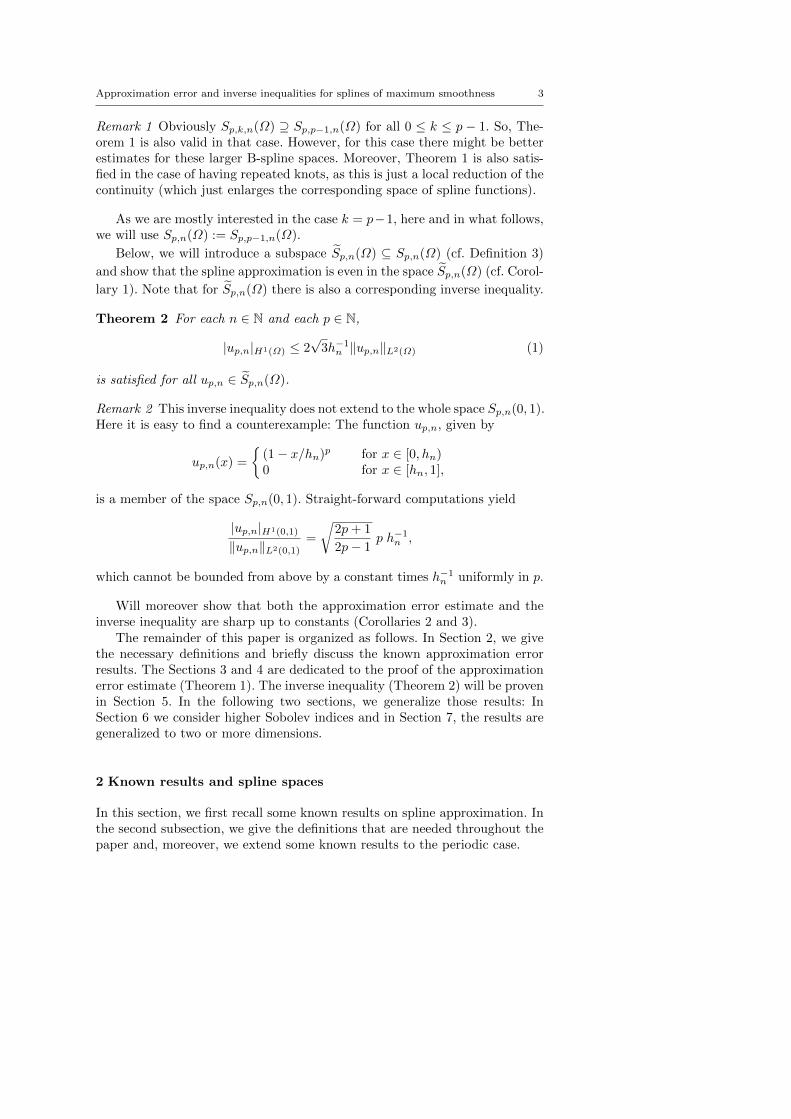
Remark 1 Obviously Sp,k,n(Ω) ⊇ Sp,p−1,n(Ω) for all 0 ≤ k ≤ p − 1. So, The-orem 1 is also valid in that case. However, for this case there might be betterestimates for these larger B-spline spaces. Moreover, Theorem 1 is also satis-fied in the case of having repeated knots, as this is just a local reduction of thecontinuity (which just enlarges the corresponding space of spline functions).

As we are mostly interested in the case k = p−1, here and in what follows,we will use Sp,n(Ω) := Sp,p−1,n(Ω).

Below, we will introduce a subspace Sp,n(Ω) ⊆ Sp,n(Ω) (cf. Definition 3)

and show that the spline approximation is even in the space Sp,n(Ω) (cf. Corol-

lary 1). Note that for Sp,n(Ω) there is also a corresponding inverse inequality.

Theorem 2 For each n ∈ N and each p ∈ N,

|up,n|H1(Ω) ≤ 2√

3h−1n ‖up,n‖L2(Ω) (1)

is satisfied for all up,n ∈ Sp,n(Ω).

Remark 2 This inverse inequality does not extend to the whole space Sp,n(0, 1).Here it is easy to find a counterexample: The function up,n, given by

up,n(x) =

(1− x/hn)p for x ∈ [0, hn)0 for x ∈ [hn, 1],

is a member of the space Sp,n(0, 1). Straight-forward computations yield

|up,n|H1(0,1)

‖up,n‖L2(0,1)=

√2p+ 1

2p− 1p h−1n ,

which cannot be bounded from above by a constant times h−1n uniformly in p.

Will moreover show that both the approximation error estimate and theinverse inequality are sharp up to constants (Corollaries 2 and 3).

The remainder of this paper is organized as follows. In Section 2, we givethe necessary definitions and briefly discuss the known approximation errorresults. The Sections 3 and 4 are dedicated to the proof of the approximationerror estimate (Theorem 1). The inverse inequality (Theorem 2) will be provenin Section 5. In the following two sections, we generalize those results: InSection 6 we consider higher Sobolev indices and in Section 7, the results aregeneralized to two or more dimensions.

2 Known results and spline spaces

In this section, we first recall some known results on spline approximation. Inthe second subsection, we give the definitions that are needed throughout thepaper and, moreover, we extend some known results to the periodic case.


2.1 Known approximation results

We start with a well-known approximation error estimate which relates – for afixed polynomial degree p and a fixed smoothness k – the approximation errorand the grid size. The result is well-known in literature, cf. [14], Theorem 6.25or [8], Theorem 7.3. In the framework of Isogeometric Analysis, such resultshave been used, e.g., in [1], Lemma 3.3.

Theorem 3 For each r ∈ N0 := 0, 1, 2, 3, . . ., each k ∈ N0, each q ∈ N andeach p ∈ N, with 0 ≤ r ≤ q ≤ p + 1 and r − 1 ≤ k < p, there is for eachu ∈ Hq(Ω) a spline approximation up,k,n ∈ Sp,k,n(Ω) such that

|u− up,k,n|Hr(Ω) ≤ C(p, k, r, q)hq−rn |u|Hq(Ω)

is satisfied, where C(p, k, r, q) is a constant that might depend on p, k, r andq. C(p, k, r, q) is independent of the gird size hn.

This lemma is valid for tensor-product spaces in any dimension and gives alocal bound for locally quasi-uniform knot vectors. However, the dependenceof the constant on the polynomial degree has not been derived.

A major step towards p-dependent estimates was presented in [2], Theo-rem 2, where an estimate with an explicit dependence on p, k, r and q wasgiven. However, there the continuity is limited by the upper bound 1

2 (p − 1).In our notation, the theorem reads as follows.

Theorem 4 For each r ∈ N0, each k ∈ N0, each q ∈ N and each p ∈ N with0 ≤ r ≤ k + 1 ≤ q ≤ p + 1 and k ≤ 1

2 (p − 1), there is for each u ∈ Hq(Ω) aspline approximation up,k,n ∈ Sp,k,n(Ω) such that

|u− up,k,n|Hr(Ω) ≤ Chq−rn (p− k)−(q−r)|u|Hq(Ω)

is satisfied, where C is a constant that is independent of p, k, r, q and the gridsize hn.

Remark 3 The requirement q ≥ k + 1 can be dropped easily. First note that

Π(r)p,k,n, the Hr-orthogonal projection operator from Hr(Ω) to Sp,k,n(Ω), is the

optimal interpolation and satisfies both,

|u−Π(r)p,k,nu|Hr(Ω) ≤ Chq−rn (p− k)−(q−r)|u|Hq(Ω) and

|u−Π(r)p,k,nu|Hr(Ω) ≤ |u|Hr(Ω).

Due to the Hilbert space interpolation theorem (Theorem 3.2.23 in [6]), weobtain that

|u−Π(r)p,k,nu|Hr(Ω) ≤ CC(q−r)/(q−r)hq−rn (p− k)−(q−r)|u|H q(Ω)

holds for any (real) q that satisfies r ≤ q ≤ q. Here, C only depends on q.


Again, the original result was stated for locally quasi-uniform knots. Forany p > 3 the relevant case k = p − 1, which we consider, is not covered bythis theorem.

Similar results to Theorem 1 are known in approximation theory, cf. [13].There, however, different norms have been discussed. Hence we do not go intothe details.

In [10], it was suggested and confirmed by numerical experiments thatTheorem 1 is satisfied. A proof was however not given.

2.2 Spline spaces

For any function u ∈ H1(0, 1), the symmetric function w : (−1, 1)→ R, givenby w(x) := u(|x|), also satisfies w ∈ H1(−1, 1). Because w(−1) = w(1), thefunction w can be extended in a periodic way to R.

The periodic extension is still symmetric, i.e. w(−x) = w(x) for all x ∈ R,and can be approximated by a periodic and symmetric spline. Here and inwhat follows, the term symmetric spline refers to a spline that is an evenfunction, i.e., to a spline satisfying wp,n(x) = wp,n(−x). The space of periodicsplines is given by the following definition.

Definition 2 Sperp,n (−1, 1) is the space of all wp,n ∈ Sp,n(−1, 1) that satisfythe periodicity condition

∂l

∂xlwp,n(−1) =

∂l

∂xlwp,n(1) for all l ∈ N0 with l < p. (2)

The restriction of a symmetric spline function wp,n ∈ Sperp,n (−1, 1) to theinterval (0, 1) is again a function in up,n ∈ Sp,n(0, 1). However, we know more:As wp,n is assumed to be a symmetric spline, i.e. an even function, we have

∂l

∂xlwp,n(x) = (−1)l

∂l

∂xlwp,n(−x) for all l ∈ N0.

By plugging x = 0 into this condition, we obtain that all odd derivatives vanishfor x = 0. By plugging x = 1 into the condition, we obtain together with (2)that also for x = 1 all odd derivatives vanish.

Concluding, the restricted function up,n is the member of some space

Sp,n(0, 1), which can be characterized by the following definition.

Definition 3 Sp,n(0, 1) is the space of all up,n ∈ Sp,n(0, 1) that satisfy thefollowing symmetry condition:

∂2l+1

∂x2l+1up,n(0) =

∂2l+1

∂x2l+1up,n(1) = 0 for all l ∈ N0 with 2l + 1 < p.

We can extend Theorem 3 for k = p − 1 to the following lemma statingthat the approximation error estimate is still satisfied if we restrict ourselves


to periodic splines. Let Hq,per(−1, 1) be the space of all w ∈ Hq(−1, 1) thatsatisfy the periodicity condition

∂l

∂xlw(−1) =

∂l

∂xlw(1) for all l ∈ N0 with l < q.

The following lemma holds.

Lemma 1 For each r ∈ N0, each q ∈ N and each p ∈ N with 0 ≤ r ≤ q ≤ p+1and r − 1 < p, there is for each w ∈ Hq,per(−1, 1) a spline approximationwp,n ∈ Sperp,n (−1, 1) such that

|w − wp,n|Hr(−1,1) ≤ C(p, r, q)hq−rn |w|Hq(−1,1)

is satisfied, where C(p, r, q) is a constant that might depend on p, r and q.C(p, r, q) is independent of the gird size hn.

Proof We make use of the fact that the proof in [14] uses local projections. So,there is a local approximation error estimate available, cf. [14], Theorem 6.24:The value of the approximation Qp,nw of a function w at a certain elementIi := (xi, xi+1) only depends on the values of the function to be approximated

in a certain neighborhood Ii := (xi − p hn, xi+1 + p hn). We assume that the

grid is fine enough such that Ii ⊆ (xi − 12 , xi + 1

2 ). Due to [14], Theorem 6.24,the following local estimate

|w −Qp,kw|Hr(Ii) ≤ C(p, r, q)hq−rn |w|Hq(Ii). (3)

is satisfied for a constant C(p, r, q) which is independent of the grid size hn.The function w can be extended periodically to R. For this function, we

can construct a spline approximation wp,n := Qp,kw, defined on R. Based on

the local error estimates (3) and using Ii ⊆ (xi − 12 , xi + 1

2 ), we obtain

|w − wp,n|Hr(−1,1) ≤ C(p, r, q) p hq−rn |w|Hq(−3/2,3/2).

Because w is periodic, we obtain

|w − wp,n|Hr(−1,1) ≤ 2 C(p, r, q) p hq−rn |w|Hq(−1,1).

This finishes the proof. ut

The next step is to introduce bases for the B-spline spaces which we havedefined in this section to make it easier to work with them and to make thereader more familiar with the function spaces. For the construction of thebasis we assume that n > p, i.e., that the grid is fine enough not to have basisfunctions that interact with both end points of the grid. Note that we do notneed this requirement for the proofs of the main theorems.

On R, B-spline basis functions (cardinal B-splines) are typically defined asfollows, cf. [14], (4.22).


Definition 4 The B-splines of degree p = 0 are given for any n ∈ N by

ψ(i)0,n(x) =

1 for x ∈ (ihn, (i+ 1)hn],0 else,

where i ∈ Z. The B-splines of degree p > 0 are for any n ∈ N given by therecurrence formula

ψ(i)p,n(x) =

x− i hnp hn

ψ(i)p−1,n(x) +

(p+ i+ 1) hn − xp hn

ψ(i+1)p−1,n(x), (4)

where i ∈ Z.

We obtain by construction that supp ψ(i)p,n = [ihn, (i+ 1 + p)hn] or, equiv-

alently, that for i ∈ −p, n the intersection of the support with Ω = (0, 1) isnon-empty.

For Sperp,n (0, 1), we introduce a B-spline basis as follows:

ϕ(i)p,n := ψ(i)

p,n + ψ(i−n)p,n : i = 1, . . . , n. (5)

To show that this is actually a basis, we observe that the functions ϕ(i)p,n are

linear independent because the cardinal B-spline functions ψ(i)p,n are linear in-

dependent and each function ψ(i)p,n only contributes to one of the functions

ϕ(i)p,n. The number of functions in (5) is n, so it coincides with the dimension

of Sp,n(0, 1) minus the number of periodicity conditions. Hence we concludethat (5) is a basis. If we omit the functions which vanish in (0, 1), we obtain

ϕ(i)p,n = ψ(i)

p,n : i = 1, . . . , n−p−1∪ϕ(i)p,n = ψ(i)

p,n+ψ(i−n)p,n : i = n−p, . . . , n.

For Sp,n(0, 1), we may introduce a B-spline basis as follows:

ψ(−i−p−1)p,n + ψ(i)

p,n + ψ(−i+2n−p+1)p,n : i = −

⌈p2

⌉, . . . , n−

⌊p2

⌋.

Again, after omitting the vanishing terms and eliminating duplicates, we derivefor odd p the basis

ψ(−(p+1)/2)p,n

∪ ψ(i)p,n + ψ(−i−p−1))

p,n : i = −(p− 1)/2, . . . ,−1

∪ ψ(i)p,n : i = 0, . . . , n− p

∪ ψ(i)p,n + ψ(−i+2n−p+1))

p,n : i = n− p+ 1, . . . , n− (p+ 1)/2

∪ ψ(n−(p−1)/2)p,n

and for even p the basis

ψ(i)p,n + ψ(−i−(p+1))

p,n : i = −p/2, . . . ,−1

∪ ψ(i)p,n : i = 0, . . . , n− p

∪ ψ(i)p,n + ψ(n−(p−1)−i)

p,n : i = n− p+ 1, . . . , n− p/2.


0 1 2 3 4 5

0.2

0.4

0.6

0.8

1.0

0 1 2 3 4 5

0.2

0.4

0.6

0.8

1.0

Fig. 1 B-spline basis functions for S1,n(0, 1) and S2,n(0, 1)

0 1 2 3 4 5

0.2

0.4

0.6

0.8

1.0

0 1 2 3 4 5

0.2

0.4

0.6

0.8

1.0


Again, we observe that these functions are linear independent. Moreover, wesee that the dimension of the space corresponds to the dimension of Sp,nminus the number of 2 bp/2c boundary conditions. This again indicates thatthe presented sets are bases.

Remark 4 By construction, the latter bases for Sp,n(0, 1) form a partition ofunity. Moreover, all basis functions are obviously non-negative.

Fig. 1 and 2 depict the B-spline basis functions that span Sp,n(0, 1). Here,the basis functions that have an influence at the boundary are plotted withsolid lines. The basis functions that have zero derivatives up to order p − 1at the boundary coincide with standard B-spline functions. They are plottedwith dashed lines.

If we compare the pictures of the B-spline basis functions in Sp,n(0, 1)(Fig. 1 and 2) with the standard B-spline basis functions for Sp,n(0, 1) (Fig. 3and 4) obtained from a classical open knot vector, we see that the latter oneshave more basis functions that are associated with the boundary. This canalso be seen by counting the number of degrees of freedom, cf. Table 1.

3 An estimate for two consecutive grids

In this section we will show an approximation error estimate for two consecu-tive grids for the periodic case. To be able to do a proper telescoping argument,


0 1 2 3 4 5

0.2

0.4

0.6

0.8

1.0

0 1 2 3 4 5

0.2

0.4

0.6

0.8

1.0


0 1 2 3 4 5

0.2

0.4

0.6

0.8

1.0

1 2 3 4 5

0.2

0.4

0.6

0.8

1.0


dim Sp,n(0, 1) dim Sperp,n (0, 1) dim Sp,n(0, 1)

p even n + p n np odd n + p n n + 1

Table 1 Degrees of freedom, where n is the number of elements and n + 1 is the numberof nodes.

we have to analyze a fixed interpolation operator. So, we show that

‖(I −Πp,n)wp,2n‖L2(−1,1) ≤√

2 hn|wp,2n|H1(−1,1) (6)

holds for all wp,2n ∈ Sperp,2n(−1, 1), where I is the identity and Πp,n is the

H1-orthogonal projection operator, given by the following definition.

Definition 5 For each w ∈ H1,per(−1, 1), Πperp,nw is the solution of the fol-

lowing problem. Find wp,n ∈ Sperp,n (−1, 1) such that

(wp,n, wp,n)H1(−1,1) = (w, wp,n)H1(−1,1)

for all wp,n ∈ Sperp,n (−1, 1), where

(u, v)H1(−1,1) := (u′, v′)L2(−1,1) +

(∫ 1

−1u(x)dx

)(∫ 1

−1v(x)dx

).


The proof will be done using Fourier analysis. For this purpose, we haveto introduce a matrix-vector formulation of (6). Here, we follow the classicalapproaches that are used in finite element (FEM) approaches as well as in Iso-geometric Analysis (IGA). So we first introduce the standard mass matrix andgive some results. Then we introduce standard stiffness matrix and intergridtransfer matrices as it is common for standard multigrid methods.

3.1 Some results for the standard mass matrix

Using the B-spline basis, we can introduce a standard mass matrix Mp,n =

(m(i,j)p,n )2n−1i,j=0, where

m(i,j)p,k = (ϕ

(i)p,k, ϕ

(j)p,k)L2(−1,1).

For an equidistant grid, we can derive the coefficients of the mass matrixexplicitly. Due to [17], we have

m(i,j)p,n = hn

E(2p+ 1, p+ ξ)

(2p+ 1)!,

where ξ ∈ −n/2, . . . , n/2 − 1 such that i − j ≡ ξ mod n. Here, E(n, k) arethe Eulerian numbers, which satisfy the recurrence relation

E(n, k) = (n− k)E(n− 1, k − 1) + (k + 1)E(n− 1, k)

and the initial condition

E(0, j) =

1 for j = 00 for j 6= 0

.

The following lemma relates the mass matrices for two polynomial degrees.

Lemma 2 For all p ∈ N, all n ∈ N and all vectors wn ∈ R2n, the inequality

‖wn‖Mp,n ≤ 2‖wn‖Mp−1,n (7)

is satisfied.

Proof Take σ := min0,minwn and define un := wn − σen, where en :=(1, 1, 1, . . .)T ∈ R2n. Then we have for q ∈ p− 1, p

‖wn‖2Mq,n= ‖un‖2Mq,n

− 2σ(un,Mq,nen)`2 + σ2(en,Mq,nen)`2 .

As the B-splines form a partition of unity (Theorem 4.20 in [14]), we haveMq,nen = h−1n en, so

‖wn‖2Mq,n= ‖un‖2Mq,n

− 2σh−1n (un, en)`2 + σ2h−1n (en, en)`2 .

Note that σ ≤ 0 and un ≥ 0. So, −2σh−1n (un, en)`2 + σ2h−1n (en, en)`2 ≥ 0.Hence (7) is a consequence of

‖un‖Mp,n≤ 2‖un‖Mp−1,n

. (8)


For un = (ui)2n−1i=0 and q ∈ p− 1, p, we have

‖un‖2Mq,n=

∫ 1

0

fq(x)2dx, with fq(x) :=

n∑i=0

uiϕ(i)q,n(x),

where the basis function ϕ(i)q,n are as specified in (5). Using the recurrence

formula (4), we obtain

fp(x) =

2n−1∑i=0

uiϕ(i)p,n(x)

=

2n−1∑i=0

ui

(x− ihnphn

ϕ(i)p−1,n(x) +

(p+ i+ 1)hn − xphn

ϕ(i−1)p−1,n(x)

)=

2n−1∑i=0

( x− ihnphn︸︷︷︸Ai :=

ui +(p+ i)hn − x

phn︸︷︷︸Bi :=

ui−1

)ϕ(i)p−1,n(x).

We have (by construction) that ϕ(i)p−1,n(x) ≥ 0, ui ≥ 0 and ui−1 ≥ 0. Moreover,

on the support of ϕ(i)p−1,n(x) we have Ai ≤ 1 and Bi ≤ 1. So we obtain

fp(x) ≤2n−1∑i=0

(ui + ui−1)ϕ(i)p−1,n(x) =

2n−1∑i=0

(un + Snun)iϕ(i)p−1,n(x),

where Sn is a shift operator, mapping (u0, u1, . . . , un−1) to (un−1, u0, . . . , un−2).Hence we conclude

‖un‖Mp,n=

(∫ 1

0

f2p (x)dx

)1/2

≤ ‖un + Snun‖Mp−1,n

≤ ‖un‖Mp−1,n + ‖Snun‖Mp−1,n = 2‖un‖Mp−1,n ,

where the last equation is due to the fact that Mp−1,n is a simple, periodicband-matrix. This finishes the proof. ut

3.2 Fourier analysis and the symbol of the mass matrix

A. Brandt has proposed to use Fourier series to analyze multigrid methods, cf.[5]. Fourier analysis provides a framework to determine sharp bounds for theconvergence rates of multigrid methods and other iterative solvers for problemsarising from partial differential equations. This is different to classical analysis,which typically yields qualitative statements only. For a detailed introductioninto Fourier analysis, see, e.g., [16].

Besides the analysis of multigrid solvers, the idea of Fourier analysis canbe carried over to the computation of approximation error estimates, as wewill see in the remainder of this section.


The key idea of Fourier analysis is to represent the vectors un ∈ Rn interms of a Fourier series

un =∑θ∈Θn

un,θ (eiθl)2n−1l=0︸︷︷︸φn(θ) :=

,

where Θn := 0, hnπ, 2hnπ, 3hnπ, . . . , (2n− 1)hnπ. We observe that

Mp,nφn(θ) = hn

p∑l=−p

E(2p+ 1, p+ l)

(2p+ 1)!eiθl︸︷︷︸

Mp,n(θ) :=

φn(θ) (9)

is satisfied, i.e., that φn(θ) is an eigenvector of Mp,n. In Fourier analysis, the

eigenvalue Mp,n(θ) is called the symbol of Mp,n.

As the factor E(2p+1,p+l)(2p+1)! in (9) is symmetric in l, we have

Mp,n(θ) = hn

p∑l=−p

E(2p+ 1, p+ l)

(2p+ 1)!cos(lθ). (10)

The symbol is better characterized by the following lemma.

Lemma 3 Mp,n(θ) ≥ 0 for all θ. Moreover, Mp,n(θ1) ≤ Mp,n(θ2) for all θ1and θ2 where cos θ1 ≤ cos θ2.

Proof For c ∈ [0, 2], we define

fp,n(c) := h−1n Mp,n(arccos(c− 1)).

The statement of the lemma is now equivalent to

– h−1n Mp,n(arccos(−1)) = fp,n(0) > 0 and

– h−1n Mp,n(arccos(c− 1)) = fp,n(c) is monotonically increasing for c > 0.

Since we can express cos(l arccos(c)) as the l-th Chebyshev polynomial, fp,nis a polynomial function in c. Using the recurrence relation for the Euleriannumbers, we can derive the following recurrence formula for fp,n:

fp,n(c) =1 + cp

1 + 2pfp−1,n(c) +

(2− c)(1 + c(−1 + 2p))

p(1 + 2p)f ′p−1,n(c)

+(−2 + c)2c

p(1 + 2p)f ′′p−1,n(c).

We can make an ansatz

fp,n(c) =

p∑j=0

ap,jcj ,


and derive the recurrence formula

ap,j =(1− j + p)2

p+ 2p2︸︷︷︸Ap,j :=

ap−1,j−1+4j(p− j) + j + p

p+ 2p2︸︷︷︸Bp,j :=

ap−1,j+2 + 6j + 4j2

p+ 2p2︸︷︷︸Cp,j :=

ap−1,j+1

for the coefficients ap,j . For p = 1, we obtain

a1,j =

13 for j ∈ 0, 10 otherwise.

As Ap,j ≥ 0, Bp,j ≥ 0 and Cp,j ≥ 0 for 0 ≤ j ≤ p, one can show usinginduction in p that for all p ≥ 1:

ap,j > 0 for j ∈ 0, 1, . . . , pap,j = 0 otherwise.

This immediately implies that fp,n(0) > 0 and that fp,n(c) is monotonicallyincreasing for c > 0, which concludes the proof. ut

3.3 The symbol of the stiffness matrix

The next step is to derive the symbol of the stiffness matrixKp,n = (k(i,j)p,n )2n−1i,j=0,

wherek(i,j)p,n =

(ϕ(i)p,n, ϕ

(j)p,n

)H1(−1,1)

.

Since the basis functions ϕ(i)p,n form a partition of unity,

∫ 1

−1 ϕ(i)p,n(x)dx = hn

holds for all i. So, we obtain

k(i,j)p,n =

(∂

∂xϕ(i)p,n,

∂

∂xϕ(j)p,n

)L2(−1,1)

+ h2n.

Note that for uniform knot vectors the identity

∂

∂xϕ(j)p,n(x) =

1

hn

(ϕ(j−1)p−1,n(x)− ϕ(j)

p−1,n(x))

holds, see e.g. (5.36) in [14]. Hence we directly obtain

k(i,j)p,n =1

h2n

(m

(i,j)p−1,n −m

(i,j−1)p−1,n −m

(i−1,j)p−1,n +m

(i−1,j−1)p−1,n

)+ h2n.

Because the grid is equidistant, this reduces to

k(i,j)p,n =1

h2n

(2m

(i,j)p−1,n −m

(i,j−1)p−1,n −m

(i−1,j)p−1,n

)+ h2n.

As∑2n−1l=0 eiθlh2n = 0 for all θ ∈ Θn\0, the term “+h2n” does not have any

effect in this case. So, the symbol of the stiffness matrix Kp,n is given via

Kp,n(θ) =2− eiθ − e−iθ

h2nMp−1,n(θ) = 2

1− cos θ

h2nMp−1,n(θ)

for θ ∈ Θn\0. For θ = 0, the part representing the derivatives vanishes and

we obtain Kp,n(0) = h2n∑2n−1l=0 e0 = 2nh2n = 2hn.


3.4 Representing intergrid transformations in Fourier analysis

As we have been mentioning in the beginning of this section, we are interestedin showing that

‖(I −Πperp,n )up,2n‖L2(−1,1) ≤

√2hn|up,2n|H1(−1,1), (11)

is satisfied for any up,2n ∈ Sperp,2n(−1, 1). Using mass matrix Mn and stiffnessmatrix Kn, this can be rewritten as

‖(I − Pp,2nK−1p,nPTp,2nKp,2n)u2n‖Mp,2n ≤√

2hn‖u2n‖Kp,2n

for all u2n ∈ R4n. Here, Pp,2n is the matrix representing the canonical embed-ding of Sperp,n (−1, 1) into Sperp,2n(−1, 1). Before we can analyze (11), we have todetermine the symbol for Pp,2n.

The following lemma is rather well-known in literature, cf. [7] equation(4.3.4), and can be easily shown by induction in p.

Lemma 4 For all p ∈ N, all n ∈ N and all x ∈ R,

ϕ(j)p,2n(x) = 2−p

p+1∑l=0

(p+ 1l

)ϕ(2j+l)p,n (x) (12)

is satisfied.

This allows to introduce the symbol of the prolongation operator. Here,the symbol cannot be understood as eigenvalue anymore as the prolongationoperator is a rectangular matrix. However, we have

φp,2n

(2θ) =

2n−1∑j=0

e2θijϕ(j)p,2n =

∑j

e2θij2−pp+1∑l=0

(p+ 1l

)ϕ(2j+l)p,n

= 2−pp+1∑l=0

(p+ 1l

)e−θil

2n−1∑j=0

eθi(2j+l)ϕ(2j+l)p,n

= 2−pp+1∑l=0

(p+ 1l

)e−θil

2n−1∑j=0

eθijϕjp,n

+ 2−pp+1∑l=0

(p+ 1l

)e−(θ+π)il

2n−1∑j=0

e(θ+π)ijϕ(j)p,n

=

(2−p

p+1∑l=0

(p+ 1l

)e−iθl

)φp,n

(θ)

+

(2−p

p+1∑l=0

(p+ 1l

)e−i(θ+π)l

)φp,n

(θ + π).


We observe that the prolongation operator Pp,2n maps the linear span, spannedby

φp,2n

(2θ) (13)

to the linear span, spanned by

φp,n

(θ) and φp,n

(θ + π). (14)

The restriction operator PTp,2n maps the linear span, spanned by (14), to thelinear span, spanned by (13). So, we can introduce the symbol as a 2×1-matrix

Pp,2n(θ) =1

2p

∑p+1l=0

(p+ 1l

)e−iθl∑p+1

l=0

(p+ 1l

)e−i(θ+π)l

=1

2p

((1 + e−iθ)p+1

(1 + e−i(θ+π))p+1

).

Now we have all the ingredients needed to derive the symbol of the projectionoperator in (11).

3.5 Analysis of the projection operator

The symbol Πperp,n (θ) of the projection operator Πper

p,n is represented in thebasis (14), i.e., it is a 2× 2-matrix with

Πperp,n (θ) = I − Pp,2n(θ)Kp,n(θ)−1Pp,2n

∗(θ)Kp,2n(θ), (15)

where A∗ is the conjugate complex of the transpose of a matrix A. Here,

Kp,2n(θ) is the representation of the symbol of the stiffness matrix correspond-ing to the basis (14). Since we know that the multiplication with the stiffnessmatrix preserves any frequency, we obtain

Kp,2n(θ) =

(Kp,2n(θ)

Kp,2n(θ + π)

),

where Kp,2n(θ) is the representation of the symbol of the stiffness matrixcorresponding to the basis (13).

The basis (14) naturally splits the domain of frequencies Θ = [0, 2π) intosubdomains Θ(high) := [π/2, 3π/2) and Θ(low) := Θ\Θ(high). Here, for anyθ ∈ Θ(low), we obtain θ+π ∈ Θ(high). We observe that cos θ ≥ 0 for θ ∈ Θ(low)

and cos θ ≤ 0 for θ ∈ Θ(high) and vice versa.Next, we show the following lemma.

Lemma 5 For any up,2n ∈ Sperp,2n(−1, 1)

‖(I −Πperp,n )up,2n‖L2(−1,1) ≤

√2hn|up,2n|H1(−1,1), (16)

is satisfied.


Proof Rewriting (16) in matrix notation, we obtain

‖M1/2p,2n(I − Pp,2nK−1p,nPTp,2nKp,2n)K

−1/2p,2n ‖ ≤

√2hn,

whereKp,n = Pp,2nKp,2nPTp,2n (Galerkin projection). Here and in what follows,

‖ · ‖ is the Euclidean norm. Using Lemma 2 we get

‖M1/2p,2n(I − Pp,2nK−1p,nPTp,2nKp,2n)K

−1/2p,2n ‖

≤ ‖M1/2p,2nM

−1/2p−1,2n‖‖M

1/2p−1,2n(I − Pp,2nK−1p,nPTp,2nKp,2n)K

−1/2p,2n ‖

≤ 2‖M1/2p−1,2n(I − Pp,2nK−1p,nPTp,2nKp,2n)K

−1/2p,2n ‖.

So it suffices to show

‖M1/2p−1,2n(I − Pp,2nK−1p,nPTp,2nKp,2n)K

−1/2p,2n ‖ ≤

1

2

√2hn,

which is equivalent to

ρ(Mp−1,2n(I − Pp,2nK−1p,nPTp,2nKp,2n)K−1p,2n) ≤ 1

2h2n, (17)

where ρ denotes the spectral radius. This statement is equivalent to

ρ(Mp−1,2n(θ)Πperp,n (θ)Kp,2n(θ)−1)︸︷︷︸

q(θ)h2n :=

≤ 1

2h2n, (18)

for all θ ∈ Θn, where Πperp,n (θ) is as defined in (15) and

Mp−1,2n(θ) =

(Mp−1,2n(θ)

Mp−1,2n(θ + π)

).

We observe that replacing θ by θ + π has the same effect as switching boththe rows and the columns of the symbol, therefore q(θ) = q(θ+π). So, we can

restrict ourselves to showing (18) for all θ ∈ Θ(low)n = Θn ∩Θ(low).

As the matrix in (18) is a 2-by-2 matrix with rank 1, the spectral radiusis equal to its trace.

From Lemma 3, we obtain that 0 ≤ Mp−1,2n(θ + π) ≤ Mp−1,2n(θ) for

all θ ∈ Θ(low)n , so we can substitute Mp−1,2n(θ + π) by ξMp−1,2n(θ), where

ξ ∈ [0, 1]. By doing this substitution, the term Mp−1,2n(θ+π) cancels out. We

obtain for θ ∈ Θ(low)n \0

q(θ) =−(1 + c)p + c(1 + c)p − (1− c)pξ − (1− c)pcξ

2(c2 − 1)((1 + c)p + (1− c)pξ),

where c := cos θ and ξ = Mp−1,2n(θ + π)/Mp−1,2n(θ). The case θ = 0 will bedealt with at the end of the proof. To finalize the proof we need to show

q(θ) ≤ 1

2


for all θ ∈ Θ(low)n \0. It suffices to show

−(1 + c)p + c(1 + c)p − (1− c)pξ − (1− c)pcξ2(c2 − 1)((1 + c)p + (1− c)pξ)

≤ 1

2

for all c ∈ ]0, 1[, all ξ ∈ [0, 1] and all p ∈ N, i.e., to show the inequality forthe whole range of all of these variables ignoring their dependence on θ. Weobserve that

0 ≤(

1− c1 + c

)p≤ 1− c

1 + c,

so there is some ω ∈ [0, 1] such that ((1− c)/(1 + c))p = (1− c)/(1 + c)ω. Aftersubstituting (1− c)p by (1− c)(1 + c)p−1ω it suffices to show

−(1 + c)p + c(1 + c)p − (1− c)(1 + c)p−1ωξ − (1− c)(1 + c)p−1ωcξ

2(c2 − 1)((1 + c)p + (1− c)(1 + c)p−1ωξ)≤ 1

2

for all c ∈ ]0, 1[, all ξ ∈ [0, 1], all ω ∈ [0, 1] and all p ∈ N. This can be simplifiedto

−(1 + c) + c(1 + c)− (1− c)ωξ − (1− c)ωcξ2(c2 − 1)((1 + c) + (1− c)ωξ)

≤ 1

2

for all c ∈ ]0, 1[, all ξ ∈ [0, 1] and all ω ∈ [0, 1]. Here the denominator is alwaysnegative. So we can multiply with the denominator and obtain

c(1− c2)(1− ωξ) ≥ 0,

which is obviously true for all c ∈ ]0, 1[, all ξ ∈ [0, 1] and all ω ∈ [0, 1].The case θ = 0 has the be considered separately. Here, we have to use

Kp,n(0) = 2hn and obtain – by straight-forward computation – that q(0) = 14 .

The inequality q(θ) ≤ 12 still holds in this case, which finishes the proof. ut

4 The proof of the approximation error estimate (Theorem 1)

First, we show the following lemma.

Lemma 6 For each w ∈ H1,per(−1, 1), each n ∈ N and each p ∈ N

‖(I −Πperp,n )w‖L2(−1,1) ≤ 2

√2 hn|w|H1(−1,1)

is satisfied.

Proof Using the triangular inequality, we obtain for any q ∈ N

‖(I −Πperp,n )w‖L2(−1,1) ≤ ‖(I −Πper

p,2qn)w‖L2(−1,1)

+

q−1∑l=0

‖(I −Πperp,2ln

)Πperp,2l+1n

w‖L2(−1,1).


We use Lemma 1 and a standard Aubin-Nitsche duality argument to estimate‖(I − Πper

p,N )w‖L2(−1,1) from above. Using [4], Lemma 7.6, and Lemma 1 forr = 1 and q = 2, we immediately obtain

‖(I −Πperp,N )w‖L2(−1,1) ≤ C(p)hN‖w‖H1(−1,1), (19)

where C(p) is independent of the grid size. Using (19) and Lemma 5, we obtain

‖(I −Πperp,n )w‖L2(−1,1) ≤ C(p) 2−qhn‖w‖H1(−1,1)

+

q−1∑l=0

√2 2−lhn|Πper

p,2l+1nw|H1(−1,1).

Because Πperp,2l+1n

is H1-orthogonal, we further obtain

‖(I −Πperp,n )w‖L2(−1,1) ≤ C(p) 2−qhn‖w‖H1(−1,1) +

q−1∑l=0

√2 2−lhn|w|H1(−1,1).

and using the summation formula for the geometric series gives

‖(I −Πperp,n )w‖L2(−1,1) ≤ C(p) 2−qhn‖w‖H1(−1,1) + 2

√2hn|w|H1(−1,1).

As this is true for all q ∈ N, we can take the limit q → ∞ and obtain thedesired result. ut

Theorem 1 is the extension of Lemma 6 to the non-periodic case.

Proof of Theorem 1 First, we observe that any u ∈ H1(0, 1) can be extendedto a w ∈ H1,per(−1, 1) by defining w(x) := u(|x|). Using Lemma 6, we canfind a function wp,n ∈ Sperp,n (−1, 1) such that

‖w − wp,n‖L2(−1,1) ≤ 2√

2 hn|w|H1(−1,1).

This function is not necessarily symmetric, i.e., wp,n(x) = wp,n(−x) might notbe true. However, wp,n(x) := 1

2 (wp,n(x) + wp,n(−x)) is symmetric and stillsatisfies the error estimate

‖w − wp,n‖L2(−1,1) ≤ 2√

2 hn|w|H1(−1,1).

By restricting wp,n to (0, 1), we obtain a function up,n ∈ Sp,n(0, 1). This func-tion satisfies the desired approximation error estimate since both |w|H1(−1,1) =√

2|u|H1(0,1) and ‖w−wp,n‖L2(−1,1) =√

2‖u−up,n‖L2(0,1) hold due to the sym-metry of w. ut

In the proof, we have defined up,n to be the restriction of a symmetric and

periodic spline wp,n to (0, 1). So, up,n ∈ Sp,n(0, 1) is satisfied, i.e., we haveshown the following result.

Corollary 1 For each u ∈ H1(0, 1), each n ∈ N and each p ∈ N, there is a

spline approximation up,n ∈ Sp,n(0, 1) such that

‖u− up,n‖L2(0,1) ≤ 2√

2 hn|u|H1(0,1)

is satisfied.


5 The proof of the inverse inequality (Theorem 2)

The proof of Theorem 2 is rather easy.

Proof of Theorem 2 We can extend every up,n ∈ Sp,n(0, 1) to (−1, 1) by defin-ing wp,n(x) := up,n(|x|) and obtain wp,n ∈ Sperp,n (−1, 1). The inverse inequal-ity (1) is equivalent to

|wp,n|H1(−1,1) ≤ 2√

3h−1n ‖wp,n‖L2(−1,1). (20)

This is shown using induction in p for all u ∈ Sp,n(−1, 1). For p = 1, (20) isknown, cf. [15], Theorem 3.91.

Now, we show that the constant does not increase for larger p. So assumep > 1 to be fixed. Due to the periodicity and due to the Cauchy-Schwarzinequality,

|wp,n|2H1(−1,1) =

∫ 1

−1(w′p,n)2dx = −

∫ 1

−1w′′p,nwp,ndx

≤ ‖w′′p,n‖L2(−1,1)‖wp,n‖L2(−1,1) = |w′p,n|H1(−1,1)‖wp,n‖L2(−1,1)

is satisfied. Using the induction assumption (and w′p,n ∈ Sperp−1,n(−1, 1), cf. [14],

Theorem 5.9), we know that

|w′p,n|H1(−1,1) ≤ 2√

3h−1n ‖w′p,n‖L2(−1,1) = Ch−1n |wp,n|H1(−1,1).

Combining these results, we obtain

|wp,n|2H1(−1,1) ≤ 2√

3h−1n |wp,n|H1(−1,1)‖wp,n‖L2(−1,1)

and further|wp,n|H1(−1,1) ≤ 2

√3h−1n ‖wp,n‖L2(−1,1).

This shows (20), which concludes the proof. ut

Remark 5 The proof of Theorem 2 does not require the grid to be equidistant.Having a general grid, the following estimate is satisfied:

|up,n|H1(0,1) ≤ 2√

3 h−1‖up,n‖L2(0,1)

for all splines up,n on (0, 1) with vanishing odd derivatives at the boundary,where h is the size of the smallest element.

As we have proven both an approximation error estimate and a correspond-ing inverse inequality, both of them are sharp (up to constants independent ofp and hn):

Corollary 2 For each n ∈ N and each p ∈ N, there is a function u ∈ H1(0, 1)such that

infup,n∈Sp,n(0,1)

‖u− up,n‖L2(0,1) ≥1

4√

3hn|u|H1(0,1) > 0.


Proof Let u ∈ Sp,n+1(0, 1) be a non-constant function with (u, up,n)L2(0,1) =0 for all up,n ∈ Sp,n. In this case, the infimum is taken for up,n = 0. So,we obtain using Theorem 2 infup,n∈Sp,n(0,1)

‖u − up,n‖L2(0,1) = ‖u‖L2(0,1) ≥1

2√3hn+1|u|H1(0,1). As hn+1 ≥ hn/2 for all n ∈ N, this finishes the proof. ut

Corollary 3 For each n ∈ N (with n ≥ 2) and each p ∈ N, there is a function

up,n ∈ Sp,n(0, 1)\0 such that

|up,n|H1(0,1) ≥1

4√

2h−1n ‖up,n‖L2(0,1).

Proof Let up,n ∈ Sp,n(0, 1)\0 be such that (up,n, up,n−1)L2(0,1) = 0 for allup,n−1 ∈ Sp,n−1. For this case ‖up,n‖L2(0,1) = infup,n−1∈Sp,n−1(0,1)

‖up,n −up,n−1‖L2(0,1) ≤ 2

√2h−1n−1|up,n|H1(0,1). As hn ≥ hn−1/2 for all n ≥ 2, this

finishes the proof. ut

6 An extension to higher Sobolev indices

We can easily lift Theorem 1 (Corollary 1) up to higher Sobolev indices.

Theorem 5 For each q ∈ N, each n ∈ N and each p ∈ N with 0 < q ≤ p+ 1,

there is for each u ∈ Hq(0, 1), a spline approximation up,n ∈ S(q)p,n(0, 1) such

that

|u− up,n|Hq−1(0,1) ≤ 2√

2 hn|u|Hq(0,1),

where S(q)p,n(0, 1) is the space of all up,n ∈ Sp,n(0, 1) that satisfy the following

symmetry condition:

∂2l+q

∂x2l+qup,n(0) =

∂2l+q

∂x2l+qup,n(1) = 0 for all l ∈ N0 with 2l + q < p.

Proof The proof is done by induction. From Corollary 1, we know the estimate

for q = 1 (as S(1)p,n(0, 1) = Sp,n(0, 1)) and all p > q − 1 = 0. For q = 1 and

p = q− 1 = 0, the estimate is a well-known result, cf. [14], Theorem 6.1, (6.7),where (in our notation) |u− u0,n|L2(0,1) ≤ hn|u|H1(0,1) has been shown.

So, now we assume to know the estimate for some q − 1 and show it for q.As u ∈ Hq(0, 1), we know that u′ ∈ Hq−1(0, 1), so we can apply the

induction hypothesis and obtain that there is some up−1,n ∈ S(q−1)p−1,n(0, 1) such

that

|u′ − up−1,n|Hq−1(0,1) ≤ 2√

2 hn|u′|Hq−1(0,1).

Define

up,n(x) := c+

∫ x

0

up−1,n(ξ)dξ. (21)

Note that up,n ∈ Sp,n(0, 1) as integrating increases both the polynomial degreeand the differentiability by 1, cf. [14], Theorem 5.16. Because by integrating


the boundary conditions on the l-th derivative become conditions on the l+1-st

derivative, we further have up,n ∈ S(q)p,n(0, 1).

Therefore, we have

|u′ − u′p,n|Hq−1(0,1) ≤ 2√

2 hn|u′|Hq−1(0,1),

which is the same as

|u− up,n|Hq(0,1) ≤ 2√

2 hn|u|Hq(0,1).

This finishes the proof. ut

Remark 6 The integration constant (integration constants for q > 2) in (21)can be used to guarantee that∫ 1

0

∂l

∂xl(u(x)− up,n(x))dx = 0

for all l ∈ 0, 1, . . . , q − 1.

For the spaces S(q)p,n(0, 1) there is again an inverse inequality.

Theorem 6 For each n ∈ N, each q ∈ N and each p ∈ N with 0 < q ≤ p+ 1,

|up,n|Hq(0,1) ≤ 2√

3h−1n |up,n|Hq−1(0,1) (22)

is satisfied for all up,n ∈ S(q)p,n(0, 1), where S

(q)p,n(0, 1) is as defined in Theorem 5.

Proof First note that (22) is equivalent to∣∣∣∣ ∂q−1∂xq−1up,n

∣∣∣∣H1(0,1)

≤ 2√

3h−1n

∥∥∥∥ ∂q−1∂xq−1up,n

∥∥∥∥L2(0,1)

. (23)

As ∂q−1

∂xq−1up,n ∈ S(1)p−q+1,n(0, 1) = Sp−q+1,n(0, 1), cf. [14], Theorem 5.9, the

estimate (23) follows directly from Theorem 2. ut

Again, as we have both an approximation error estimate and an inverseinequality, we know that both of them are sharp (cf. Corollaries 2 and 3).

The following theorem is directly obtained from telescoping.

Theorem 7 For each q ∈ N0, each n ∈ N, each p ∈ N, each r ∈ N with0 ≤ r ≤ q ≤ p + 1, there is for each u ∈ Hq(0, 1) a spline approximationup,n ∈ Sp,n(0, 1) such that

|u− up,n|Hr(0,1) ≤ (2√

2 hn)q−r|u|Hq(0,1)

is satisfied.


Proof Theorem 5 states the desired result for r = q − 1. For r < q − 1, thestatement is shown by induction in r. So, we assume to know the desired resultfor some r, i.e., there is a spline approximation up,n ∈ Sp,n(0, 1) such that

|u− up,n|Hr(0,1) ≤ (2√

2 hn)q−r|u|Hq(0,1). (24)

Now, we show that there is some up,n ∈ Sp,n(0, 1) such that

|u− up,n|Hr−1(0,1) ≤ (2√

2 hn)q−(r−1)|u|Hq(0,1). (25)

Theorem 5 states that there is a function up,n ∈ Sp,n(0, 1) such that

|u− up,n|Hr−1(0,1) ≤ 2√

2 hn|u− up,n|Hr(0,1),

which shows together with the induction assumption (24) the induction hy-pothesis (25). ut

Here, it is not known to the authors how to choose a proper subspaceof Sp,n(0, 1) such that a complementary inverse inequality can be shown.

7 Extension to two and more dimensions and application inIsogeometric Analysis

We can extend Theorem 1 (and also Corollary 1) to the following theoremfor a tensor-product structured grid on Ω := (0, 1)d. Here, we can intro-

duce Wp,n(Ω) = ⊗di=1Sp,n(0, 1). Assuming that (φ(0)p,n, . . . , φ

(N)p,n ) is a basis of

Sp,n(0, 1), the space Wp,n(Ω) is given by

Wp,n(Ω) =

w : w(x1, . . . , xd) =

N∑i1,...,id=0

wi1,...,idφ(i1)p,n (x1) · · ·φ(id)p,n (xd)

.

Theorem 8 Let Ω = (0, 1)d. For each u ∈ H1(Ω), each n ∈ N and each

p ∈ N0 there is a spline approximation wp,n ∈ Wp,n(Ω) such that

‖u− wp,n‖L2(Ω) ≤ 2√

2d hn|u|H1(Ω)

is satisfied.

The proof is similar to the proof in [3], Section 4, for the two dimensional case.To keep the paper self-contained we give a proof of this theorem.

Proof of Theorem 8 For sake of simplicity, we restrict ourselves to d = 2. Theextension to more dimensions is completely analogous. Here

Wp,n(Ω) = Sp,n(0, 1)⊗Sp,n(0, 1) =

w : w(x, y) =

N∑i,j=0

wi,jφ(i)p,n(x)φ(j)p,n(y)

.


We assume u ∈ C∞(Ω) and show the desired result using a standarddensity argument. Using Theorem 1, we can introduce for each x ∈ (0, 1) a

function v(x, ·) ∈ Sp,n(0, 1) with

‖u(x, ·)− v(x, ·)‖L2(0,1) ≤ 2√

2 hn|u(x, ·)|H1(0,1).

By squaring and taking the integral over x, we obtain

‖u− v‖L2(Ω) ≤ 2√

2 hn

∥∥∥∥ ∂∂yu∥∥∥∥L2(Ω)

. (26)

By choosing v(x, ·) to be the L2-orthogonal projection, we also have

‖v(x, ·)‖L2(0,1) ≤ ‖u(x, ·)‖L2(0,1)

for all x ∈ (0, 1) and consequently∥∥∥∥ ∂∂xv(x, ·)∥∥∥∥L2(0,1)

≤∥∥∥∥ ∂∂xu(x, ·)

∥∥∥∥L2(0,1)

. (27)

As v(x, ·) ∈ Sp,n(0, 1), there are coefficients vj(x) such that

v(x, y) =

N∑j=0

vj(x)φ(j)p,n(y).

Using Corollary 1, we can introduce for each j ∈ 0, . . . , N a function wj ∈Sp,n(0, 1) with

‖vj − wj‖L2(0,1) ≤ 2√

2 hn|vj |H1(0,1). (28)

Next, we introduce a function w by defining

w(x, y) :=

N∑j=0

wj(x)φ(j)p,n(y),

which is obviously a member of the space Wp,n(Ω). By squaring (28), multi-

plying it with φ(j)p,n(y)2, summing over j and taking the integral, we obtain∫ 1

0

N∑j=0

‖vj − wj‖2L2(0,1)φ(j)p,n(y)2dy ≤ 8 h2n

∫ 1

0

N∑j=0

|vj |2H1(0,1)φ(j)p,n(y)2dy.

Using the definition of the norms, we obtain∫ 1

0

∫ 1

0

N∑j=0

(vj(x)−wj(x))2φ(j)p,n(y)2dxdy ≤ 8 h2n

∫ 1

0

∫ 1

0

N∑j=0

v′j(x)2φ(j)p,n(y)2dxdy

and further

‖v − w‖L2(Ω) ≤ 2√

2 hn

∥∥∥∥ ∂∂xv∥∥∥∥L2(Ω)

.


Using (27), we obtain

‖v − w‖L2(Ω) ≤ 2√

2 hn

∥∥∥∥ ∂∂yu∥∥∥∥L2(Ω)

. (29)

Using (26) and (29), we obtain

‖u− w‖L2(Ω) ≤ ‖u− v‖L2(Ω) + ‖v − w‖L2(Ω)

≤ 2√

2 hn

∥∥∥∥ ∂∂yu∥∥∥∥L2(Ω)

+ 2√

2 hn

∥∥∥∥ ∂∂xu∥∥∥∥L2(Ω)

≤ 4 hn|u|H1(Ω),

which finishes the proof. ut

The extension of Theorem 2 to two or more dimensions is rather easy.

Theorem 9 Consider Ω := (0, 1)d. For each n ∈ N and each p ∈ N,

|up,n|H1 ≤ 2√

3d h−1n ‖up,n‖L2

is satisfied for all up,n ∈ Wp,n(Ω).

Proof For sake of simplicity, we restrict ourselves to d = 2. The generalizationto more dimensions is completely analogous.

We have obviously

|up,n|2H1 =

∥∥∥∥ ∂∂xup,n∥∥∥∥2L2

+

∥∥∥∥ ∂∂yup,n∥∥∥∥2L2

=

∫ 1

0

|up,n(·, y)|2H1dy +

∫ 1

0

|up,n(x, ·)|2H1dx

This can be bounded from above using Theorem 2 by

= 12h−2n

(∫ 1

0

‖up,n(·, y)‖2L2dy +

∫ 1

0

‖up,n(x, ·)‖2L2dx

)= 24h−2n ‖up,n‖2L2 ,

which finishes the proof. ut

The extension to isogeometric spaces can be done following the approachpresented in [1], Section 3.3. In Isogeometric Analysis, we have a geometryparameterization F : (0, 1)d → Ω. An isogeometric function on Ω is thengiven as the composition of a B-spline on (0, 1)d with the inverse of F. Thefollowing result can be shown using a standard chain rule argument.

There exists a constant C = C(F, q) such that

C−1 ‖f‖Hq(Ω) ≤ ‖f F‖Hq((0,1)d) ≤ C ‖f‖Hq(Ω) (30)

for all f ∈ Hq(Ω).


See [1], Lemma 3.5, or [3], Corollary 5.1, for related results. In both pa-pers the statements are slightly more general, [1] gives a more detailed depen-dence on the parameterization F whereas [3] establishes bounds for anisotropicmeshes.

Using this equivalence of norms, we can transfer all results from the pa-rameter domain (0, 1)d to the physical domain Ω. However, we need to pointout that this equivalence is not valid for seminorms. Hence, in Theorem 1 (andfollow-up Theorems 5, 7 and 8) the seminorms on the right hand side of theequations need to be replaced by the full norms. Moreover, the bounds dependon the geometry parameterization via the constant C in (30).

A similar strategy can be followed when extending the results to NURBS.We do not go into the details here but refer to [1,3] for a more detailed study.In the case of NURBS the seminorms again have to be replaced by the fullnorms due to the quotient rule of differentiation. In that case the constantsof the bounds additionally depend on the given denominator of the NURBSparameterization.

References

1. Yuri Bazilevs, Lourenco Beirao da Veiga, J Austin Cottrell, Thomas JR Hughes, andGiancarlo Sangalli, Isogeometric analysis: approximation, stability and error estimatesfor h-refined meshes, Mathematical Models and Methods in Applied Sciences 16 (2006),no. 07, 1031–1090.

2. Lourenco Beirao da Veiga, Annalisa Buffa, J Rivas, and Giancarlo Sangalli, Some es-timates for h–p–k-refinement in isogeometric analysis, Numerische Mathematik 118(2011), no. 2, 271–305.

3. Lourenco Beirao da Veiga, Durkbin Cho, and Giancarlo Sangalli, Anisotropic nurbsapproximation in isogeometric analysis, Computer Methods in Applied Mechanics andEngineering 209 (2012), 1–11.

4. Dietrich Braess, Finite elements: Theory, fast solvers, and applications in solid me-chanics (second editin), Cambridge University Press, 2001.

5. Achi Brandt, Multi-level adaptive solutions to boundary-value problems, Math. Comp.31 (1977), 333 – 390.

6. Paul Butzer and Hubert Berens, Semi-Groups of Operators and Approximation,Springer-Verlag, Berlin Heidelberg New York, 1967.

7. Charles K Chui, An introduction to wavelets, wavelet analysis and its applications,Academic Press, Boston (1992).

8. Ronald A DeVore and George G Lorentz, Constructive approximation, Die Grundlehrender mathematischen Wissenschaften in Einzeldarstellungen, Springer, 1993.

9. Marco Donatelli, Carlo Garoni, Carla Manni, Stefano Serra-Capizzano, and HendrikSpeleers, Robust and optimal multi-iterative techniques for iga galerkin linear systems,Computer Methods in Applied Mechanics and Engineering 284 (2015), no. 0, 230 – 264,Isogeometric Analysis Special Issue.

10. John A Evans, Yuri Bazilevs, Ivo Babuska, and Thomas JR Hughes, n-widths, sup–infs, and optimality ratios for the k-version of the isogeometric finite element method,Computer Methods in Applied Mechanics and Engineering 198 (2009), no. 21, 1726–1741.

11. Carlo Garoni, Carla Manni, Francesca Pelosi, Stefano Serra-Capizzano, and HendrikSpeleers, On the spectrum of stiffness matrices arising from isogeometric analysis, Nu-merische Mathematik 127 (2014), no. 4, 751–799 (English).

12. Thomas JR Hughes, J Austrin Cottrell, and Yuri Bazilevs, Isogeometric analysis: CAD,finite elements, NURBS, exact geometry and mesh refinement, Computer Methods inApplied Mechanics and Engineering 194 (2005), no. 39-41, 4135 – 4195.


13. Nicolai Korneichuk, Exact constants in approximation theory, vol. 38, Cambridge Uni-versity Press, 1991.

14. Larry L Schumaker, Spline functions: basic theory, Cambridge University Press, 1981.15. Christoph Schwab, p- and hp- finite element methods: Theory and applications in solid

and fluid mechanics, Numerical Mathematics and Scientific Computation, ClarendonPress, 1998.

16. Ulrich Trottenberg, Cornelius Oosterlee, and Anton Schuller, Multigrid, Academic Press,London, 2001.

17. Ren-Hong Wang, Yan Xu, and Zhi-Qiang Xu, Eulerian numbers: a spline perspective,Journal of Mathematical Analysis and Applications 370 (2010), no. 2, 486–490.

Latest Reports in this series2009 - 2012

[..]

2013[..]2013-08 Wolfgang Krendl, Valeria Simoncini and Walter Zulehner

Efficient Preconditioning for an Optimal Control Problem with the Time-periodic Stokes Equations

November 2013

20142014-01 Helmut Gfrerer and Jirı V. Outrata

On Computation of Generalized Derivatives of the Normal-Cone Mapping andtheir Applications

May 2014

2014-02 Helmut Gfrerer and Diethard KlatteQuantitative Stability of Optimization Problems and Generalized Equations May 2014

2014-03 Clemens Hofreither and Walter ZulehnerOn Full Multigrid Schemes for Isogeometric Analysis May 2014

2014-04 Ulrich Langer, Sergey Repin and Monika WolfmayrFunctional A Posteriori Error Estimates for Parabolic Time-Periodic Bound-ary Value Problems

July 2014

2014-05 Irina Georgieva and Clemens HofreitherInterpolating Solutions of the Poisson Equation in the Disk Based on RadonProjections

July 2014

2014-06 Wolfgang Krendl and Walter ZulehnerA Decomposition Result for Biharmonic Problems and the Hellan-Herrmann-Johnson Method

July 2014

2014-07 Martin Jakob Gander and Martin NeumullerAnalysis of a Time Multigrid Algorithm for DG-Discretizations in Time September 2014

2014-08 Martin Jakob Gander and Martin NeumullerAnalysis of a New Space-Time Parallel Multigrid Algorithm for Parabolic Prob-lems

November 2014

2014-09 Helmut Gfrerer and Jirı V. OutrataOn Computation of Limiting Coderivatives of the Normal-Cone Mapping toInequality Systems and their Applications

December 2014

2014-10 Clemens Hofreither and Walter ZulehnerSpectral Analysis of Geometric Multigrid Methods for Isogeometric Analysis December 2014

2014-11 Clemens Hofreither and Walter ZulehnerMass Smoothers in Geometric Multigrid for Isogeometric Analysis December 2014

20152015-01 Peter Gangl, Ulrich Langer, Antoine Laurain, Houcine Meftahi and Kevin

SturmShape Optimization of an Electric Motor Subject to Nonlinear Magnetostatics January 2015

2015-02 Stefan Takacs and Thomas TakacsApproximation Error Estimates and Inverse Inequalities for B-Splines of Max-imum Smoothness

February 2015

From 1998 to 2008 reports were published by SFB013. Please seehttp://www.sfb013.uni-linz.ac.at/index.php?id=reports

From 2004 on reports were also published by RICAM. Please seehttp://www.ricam.oeaw.ac.at/publications/list/

For a complete list of NuMa reports seehttp://www.numa.uni-linz.ac.at/Publications/List/

JOHANNES KEPLER UNIVERSITY LINZ Institute of Computational ... · Institute of Computational...

Documents

Transcript of JOHANNES KEPLER UNIVERSITY LINZ Institute of Computational ... · Institute of Computational...