Johannes Gutenberg-University Mainzrathgeber/Lectures/Chap4_Polymer... · Johannes...
34
Johannes Gutenberg-University Mainz Institute for Physics PD Dr. Silke Rathgeber Johannes Gutenberg-University Mainz Institute for Physics – KOMET 331 Staudingerweg 7 55099 Mainz Germany phone: +49 (0) 6131/ 392-3323 Fax: +49 (0) 6131/ 392-5441 email: [email protected] phone: +49 (0) 6131/ 392-3323 Fax: +49 (0) 6131/ 392-5441 email: [email protected] webpage: http://www.cond-mat.physik.uni-mainz.de/~rathgebs/ Chapter 4: POLYMER SOLUTIONS AND MIXTURES 4.1 Excluded volume interaction & Flory theory • idea of excluded volume interactions • θ−temperature • Flory approach for the free energy and scaling behavior of R E with excluded volume interactions Up to here (see script Chap. 3) we looked at the properties of a single chain with increasing concentration polymer will interpenetrate each other. We can distinguish the following concentration regions: Range of concentrations Overlap concentration c ∗ pervaded volume V~R 3 overlap of single polymer if 3 3 (with ν = Flory exponent) ( ) mon mon mon Nv Nv Nv c V R Nl ν ∗ = ≈ = ⇒ 13 0.8 ~ ~ c N N ν ∗ − − if 3 5 ν = for good solvent conditions. For high degrees of polymerization, the overlap concentration can be rather low! dilute solution c << c* overlap concentration c ≈ c* semi-dilute solution c > c* (actual concentration low) melt single polymer
Transcript of Johannes Gutenberg-University Mainzrathgeber/Lectures/Chap4_Polymer... · Johannes...
Johannes Gutenberg-University Mainz Institute for Physics
PD Dr. Silke Rathgeber Johannes Gutenberg-University Mainz Institute for Physics – KOMET 331 Staudingerweg 7 55099 Mainz Germany
phone: +49 (0) 6131/ 392-3323 Fax: +49 (0) 6131/ 392-5441 email: [email protected]
phone: +49 (0) 6131/ 392-3323 Fax: +49 (0) 6131/ 392-5441 email: [email protected] webpage: http://www.cond-mat.physik.uni-mainz.de/~rathgebs/
Chapter 4: POLYMER SOLUTIONS AND MIXTURES 4.1 Excluded volume interaction & Flory theory • idea of excluded volume interactions • θ−temperature • Flory approach for the free energy and scaling behavior of RE with excluded volume
interactions
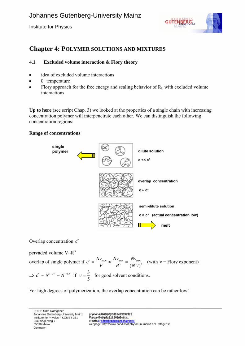
Up to here (see script Chap. 3) we looked at the properties of a single chain with increasing concentration polymer will interpenetrate each other. We can distinguish the following concentration regions: Range of concentrations
Overlap concentration c∗ pervaded volume V~R3
overlap of single polymer if 3 3 (with ν = Flory exponent)( )
mon mon monNv Nv NvcV R N lν
∗ = ≈ =
⇒ 1 3 0.8~ ~c N Nν∗ − − if 35
ν = for good solvent conditions.
For high degrees of polymerization, the overlap concentration can be rather low!
dilute solution c << c*
overlap concentration c ≈ c*
semi-dilute solution c > c* (actual concentration low)
melt
single polymer

PD Dr. Silke Rathgeber Johannes Gutenberg-University Mainz Institute for Physics – KOMET 331 Staudingerweg 7 55099 Mainz Germany
phone: +49 (0) 6131/ 392-3323 Fax: +49 (0) 6131/ 392-5441 email: [email protected] webpage: http://www.cond-mat.physik.uni-mainz.de/~rathgebs/
Now we look at the thermodynamic properties of polymers in solutions at c c∗≥ and in polymer mixtures (dense systems). i.e. phase separations & osmotic pressure Flory-Huggins theory A mixture is miscible if the free enthalpy of mixing 0mix mix mixG H T SΔ = Δ − Δ < where mixHΔ and mixSΔ are the enthalpy and entropy of mixing, respectively. First we look at a mixture of low molecular weigth substances
• distribution on lattice without change in volume • both components have lattice volume so in this theory; number fraction=volume fraction
Entropy of mixing
n1 = number of lattice sites for component 1 n2 = number of lattice sites for component 2 n=n1+n2 = total number of lattice sites Calculation of entropy change
lnmix BS kΔ = Ω where Ω = number of possible distributions of component 1 & 2 on lattice sites
1 2
!! !n
n nΩ = the denominator takes permutations of component 1&2 among each
other into account with ln ! lnx x x x≈ −
PD Dr. Silke Rathgeber Johannes Gutenberg-University Mainz Institute for Physics – KOMET 331 Staudingerweg 7 55099 Mainz Germany
phone: +49 (0) 6131/ 392-3323 Fax: +49 (0) 6131/ 392-5441 email: [email protected] webpage: http://www.cond-mat.physik.uni-mainz.de/~rathgebs/
⇒ 1 21 2ln lnmix B
n nS k n nn n
⎡ ⎤⎛ ⎞ ⎛ ⎞Δ = − +⎜ ⎟ ⎜ ⎟⎢ ⎥⎝ ⎠ ⎝ ⎠⎣ ⎦ with number fractions 1 2
1 2andn nc cn n
= =
since component 1&2 have same lattice volume: number fraction=volume fraction ⇒ ( ) ( )1 1 2 2ln lnmix BS nk c c c cΔ = − +⎡ ⎤⎣ ⎦
⇒ if n=NA ( ) ( )1 1 2 2ln lnnmixS R c c c cΔ = − +⎡ ⎤⎣ ⎦ per mole!
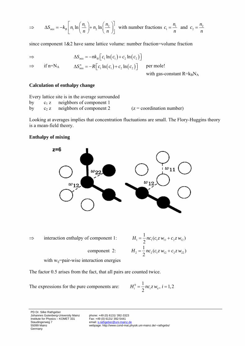
with gas-constant R=kBNA Calculation of enthalpy change Every lattice site is in the average surrounded by c1 z neighbors of component 1 by c2 z neighbors of component 2 (z = coordination number) Looking at averages implies that concentration fluctuations are small. The Flory-Huggins theory is a mean-field theory. Enthalpy of mixing
⇒ interaction enthalpy of component 1: 1 1 1 11 2 121 ( )2
H nc c z w c z w= +
component 2: 2 2 1 12 2 221 ( )2
H nc c z w c z w= +
with wij=pair-wise interaction energies The factor 0.5 arises from the fact, that all pairs are counted twice.
The expressions for the pure components are: 0 1 , 1,22i i iiH nc z w i= =
z=6
PD Dr. Silke Rathgeber Johannes Gutenberg-University Mainz Institute for Physics – KOMET 331 Staudingerweg 7 55099 Mainz Germany
phone: +49 (0) 6131/ 392-3323 Fax: +49 (0) 6131/ 392-5441 email: [email protected] webpage: http://www.cond-mat.physik.uni-mainz.de/~rathgebs/
0 01 2 1 2 1 2 12 11 22 1 2
1 2 12 12 12 11 22
1( ) ( ) (2 ) 12
1 ( )2
mixH H H H H nzc c w w w with c c
nzc c w with w w w w
Δ = + − + = − − + =
= Δ Δ = − +
⇒ 1 2 12
MmixH nzc c wΔ = Δ per mole!
12 0wΔ < exothermal mixing process
12 0wΔ > endothermal mixing process
12 0wΔ = athermal mixing process
introduction of the interaction parameter: 12 121 1w
RT Tχ = Δ ∝
⇒ 12 1 2MmixH RT c cχΔ =
⇒ free enthalpy of mixing: [ ]1 1 2 2 12 1 2ln lnM
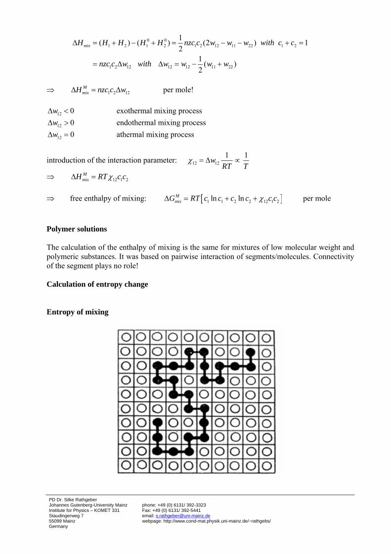
mixG RT c c c c c cχΔ = + + per mole Polymer solutions The calculation of the enthalpy of mixing is the same for mixtures of low molecular weight and polymeric substances. It was based on pairwise interaction of segments/molecules. Connectivity of the segment plays no role! Calculation of entropy change Entropy of mixing
PD Dr. Silke Rathgeber Johannes Gutenberg-University Mainz Institute for Physics – KOMET 331 Staudingerweg 7 55099 Mainz Germany
phone: +49 (0) 6131/ 392-3323 Fax: +49 (0) 6131/ 392-5441 email: [email protected] webpage: http://www.cond-mat.physik.uni-mainz.de/~rathgebs/
n1= number of solvent molecules n2= number of polymers N= lattice sites per polymer = degree of polymerization n= n1+n2N = total number of lattice sites Assume that i polymers are already distributed on the lattice ⇒ number of free sites is: n-N×i ⇒ for the first segment of the (i+1) polymer there are (n-N×i) possibilities to find a site ⇒ for the second segment there are z × (number of free sites) ⇒ for the third to xth segment there are (z-1) × (number of free sites)
number of free sites is replaced by the average number: n N in
− ×
• n>>N otherwise there would be a significant reduction with each segment added
Entropy of mixing
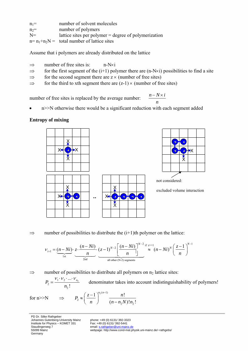
⇒ number of possibilities to distribute the (i+1)th polymer on the lattice:
2 1if z>>1
21
1st2nd all other (N-2) segments
( ) ( ) 1( ) ( 1) ( )N N
N Ni
n Ni n Ni zn Ni z z n Nin n n
ν− −
−+
− − −⎡ ⎤ ⎛ ⎞= − ⋅ ⋅ ⋅ − ≈ − ⎜ ⎟⎢ ⎥⎣ ⎦ ⎝ ⎠1424314243 14444244443
⇒ number of possibilities to distribute all polymers on n2 lattice sites:
21 22
2
...!
nPn
ν ν ν⋅ ⋅ ⋅= denominator takes into account indistinguishability of polymers!
for n>>N ⇒ 2 ( 1)
22 2
1 !( )! !
n nz nPn n n N n
−−⎛ ⎞≈ ⎜ ⎟ −⎝ ⎠
not considered: excluded volume interaction
1
X
X
X
X 4
1
3
2
X
X
X
X
X 2 1 4 3 2 1
X
X
X..
PD Dr. Silke Rathgeber Johannes Gutenberg-University Mainz Institute for Physics – KOMET 331 Staudingerweg 7 55099 Mainz Germany
phone: +49 (0) 6131/ 392-3323 Fax: +49 (0) 6131/ 392-5441 email: [email protected] webpage: http://www.cond-mat.physik.uni-mainz.de/~rathgebs/
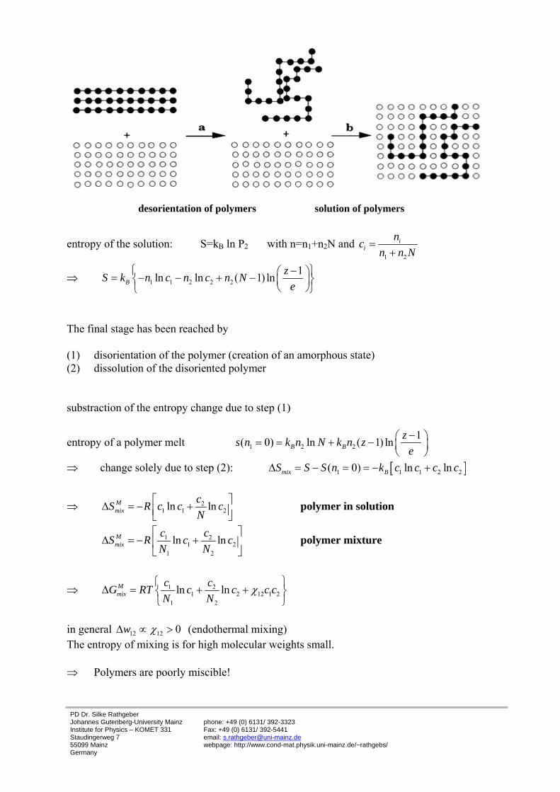
entropy of the solution: S=kB ln P2 with n=n1+n2N and 1 2
ii
ncn n N
=+
⇒ 1 1 2 2 21ln ln ( 1) lnB
zS k n c n c n Ne
⎧ − ⎫⎛ ⎞= − − + −⎨ ⎬⎜ ⎟⎝ ⎠⎩ ⎭
The final stage has been reached by (1) disorientation of the polymer (creation of an amorphous state) (2) dissolution of the disoriented polymer substraction of the entropy change due to step (1)
entropy of a polymer melt 1 2 21( 0) ln ( 1) lnB B
zs n k n N k n ze−⎛ ⎞= = + − ⎜ ⎟
⎝ ⎠
⇒ change solely due to step (2): [ ]1 1 1 2 2( 0) ln lnmix BS S S n k c c c cΔ = − = = − +
⇒ 21 1 2ln lnM
mixcS R c c cN
⎡ ⎤Δ = − +⎢ ⎥⎣ ⎦ polymer in solution
1 21 2
1 2
ln lnMmix
c cS R c cN N
⎡ ⎤Δ = − +⎢ ⎥
⎣ ⎦ polymer mixture
⇒ 1 21 2 12 1 2
1 2
ln lnMmix
c cG RT c c c cN N
χ⎧ ⎫
Δ = + +⎨ ⎬⎩ ⎭
in general 12 12 0w χΔ ∝ > (endothermal mixing) The entropy of mixing is for high molecular weights small. ⇒ Polymers are poorly miscible!
desorientation of polymers solution of polymers
PD Dr. Silke Rathgeber Johannes Gutenberg-University Mainz Institute for Physics – KOMET 331 Staudingerweg 7 55099 Mainz Germany
phone: +49 (0) 6131/ 392-3323 Fax: +49 (0) 6131/ 392-5441 email: [email protected] webpage: http://www.cond-mat.physik.uni-mainz.de/~rathgebs/
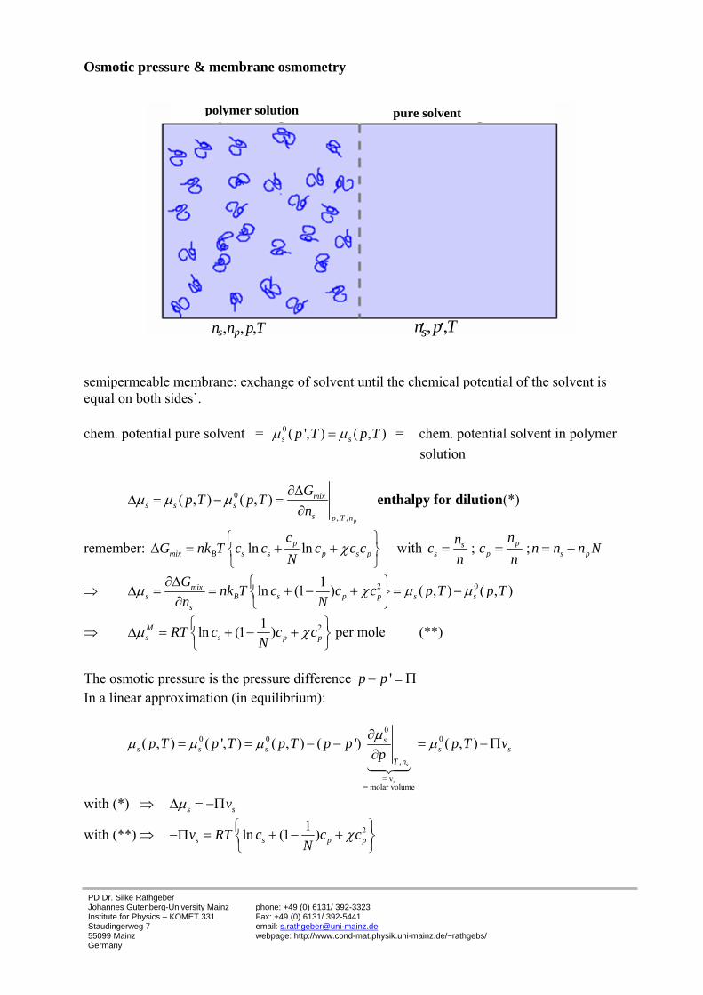
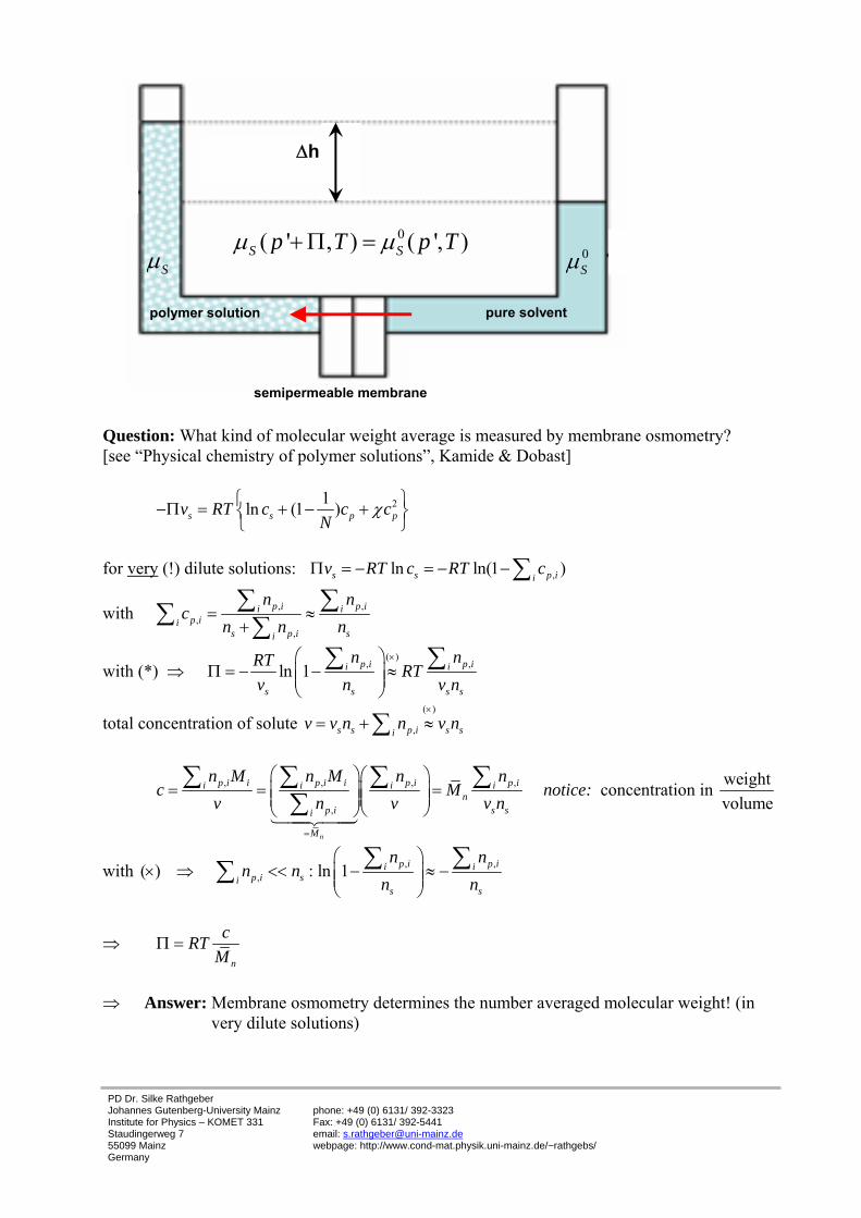
Osmotic pressure & membrane osmometry
semipermeable membrane: exchange of solvent until the chemical potential of the solvent is equal on both sides`. chem. potential pure solvent = 0 ( ', ) ( , )s sp T p Tμ μ= = chem. potential solvent in polymer solution
0
, ,
( , ) ( , )p
mixs s s
s p T n
Gp T p Tn
μ μ μ ∂ΔΔ = − =
∂ enthalpy for dilution (*)
remember: ln lnpmix B s s p s p
cG nk T c c c c c
Nχ
⎧ ⎫Δ = + +⎨ ⎬
⎩ ⎭ with ; ;ps
s p s p
nnc c n n n Nn n
= = = +
⇒ 2 01ln (1 ) ( , ) ( , )mixs B s p p s s
s
G nk T c c c p T p Tn N
μ χ μ μ∂Δ ⎧ ⎫Δ = = + − + = −⎨ ⎬∂ ⎩ ⎭
⇒ 21ln (1 )Ms s p pRT c c c
Nμ χ⎧ ⎫Δ = + − +⎨ ⎬
⎩ ⎭ per mole (**)
The osmotic pressure is the pressure difference 'p p− = Π In a linear approximation (in equilibrium):
s
00 0 0
,
= v= molar volume
( , ) ( ', ) ( , ) ( ') ( , )s
ss s s s s
T n
p T p T p T p p p T vp
μμ μ μ μ∂= = − − = − Π
∂14243
with (*) ⇒ s svμΔ = −Π
with (**) ⇒ 21ln (1 )s s p pv RT c c cN
χ⎧ ⎫−Π = + − +⎨ ⎬⎩ ⎭
polymer solution pure solvent
, , ,s pn n p T , ,sn p T′ ′
PD Dr. Silke Rathgeber Johannes Gutenberg-University Mainz Institute for Physics – KOMET 331 Staudingerweg 7 55099 Mainz Germany
phone: +49 (0) 6131/ 392-3323 Fax: +49 (0) 6131/ 392-5441 email: [email protected] webpage: http://www.cond-mat.physik.uni-mainz.de/~rathgebs/
for low polymer concentrations 211: ln ln(1 ) ...2p s p p pc c c c c<< = − ≈ − − +
⇒ 21 ...2
ps p
cv RT c
Nχ
⎧ ⎫⎛ ⎞−Π = + − +⎨ ⎬⎜ ⎟⎝ ⎠⎩ ⎭
with ps
cv RT
NΠ = van’t Hoff Law
and the other terms are derivations from ideal behavior, they disappear for 12
χ =
remember: (1) 1Tχ −∝ (2) osmotic pressure is the pressure difference between polymer solution and pure solution ⇒
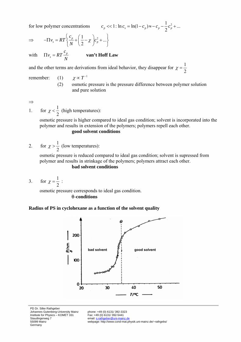
1. for 12
χ < (high temperatures):
osmotic pressure is higher compared to ideal gas condition; solvent is incorporated into the polymer and results in extension of the polymers; polymers repell each other. good solvent conditions
2. for 12
χ > (low temperatures):
osmotic pressure is reduced compared to ideal gas condition; solvent is supressed from polymer and results in strinkage of the polymers; polymers attract each other. bad solvent conditions
3. for 12
χ = :
osmotic pressure corresponds to ideal gas condition. θ-conditions
Radius of PS in cyclohexane as a function of the solvent quality
good solvent bad solvent
PD Dr. Silke Rathgeber Johannes Gutenberg-University Mainz Institute for Physics – KOMET 331 Staudingerweg 7 55099 Mainz Germany
phone: +49 (0) 6131/ 392-3323 Fax: +49 (0) 6131/ 392-5441 email: [email protected] webpage: http://www.cond-mat.physik.uni-mainz.de/~rathgebs/
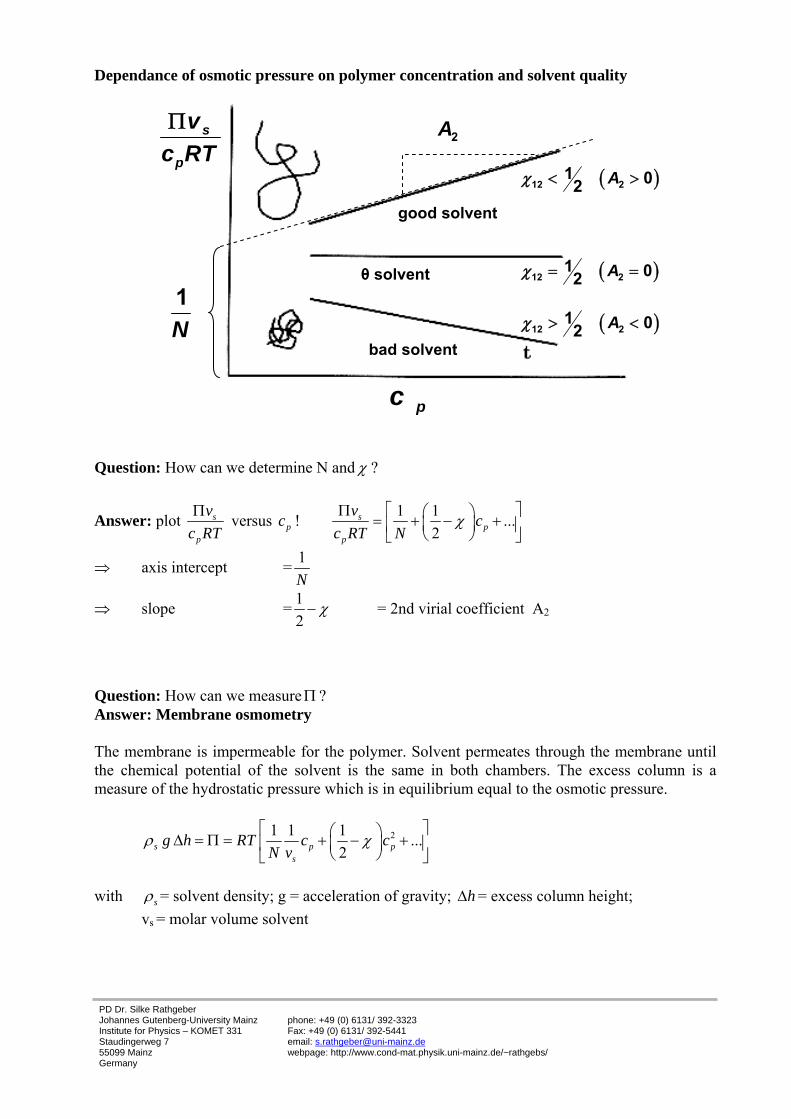
Dependance of osmotic pressure on polymer concentration and solvent quality
Question: How can we determine N and χ ?
Answer: plot s
p
vc RTΠ versus pc ! 1 1 ...
2s
pp
v cc RT N
χΠ ⎡ ⎤⎛ ⎞= + − +⎜ ⎟⎢ ⎥⎝ ⎠⎣ ⎦
⇒ axis intercept = 1N
⇒ slope = 12
χ− = 2nd virial coefficient A2
Question: How can we measure Π ? Answer: Membrane osmometry The membrane is impermeable for the polymer. Solvent permeates through the membrane until the chemical potential of the solvent is the same in both chambers. The excess column is a measure of the hydrostatic pressure which is in equilibrium equal to the osmotic pressure.
21 1 1 ...2s p p
s
g h RT c cN v
ρ χ⎡ ⎤⎛ ⎞Δ = Π = + − +⎢ ⎥⎜ ⎟
⎝ ⎠⎣ ⎦
with sρ = solvent density; g = acceleration of gravity; hΔ = excess column height; vs = molar volume solvent
s
p
vc RTΠ
pc
bad solvent
good solvent
θ solvent
( )12 21 02 Aχ < >
( )12 21 02 Aχ = =
( )12 21 02 Aχ > <
1N
2A
PD Dr. Silke Rathgeber Johannes Gutenberg-University Mainz Institute for Physics – KOMET 331 Staudingerweg 7 55099 Mainz Germany
phone: +49 (0) 6131/ 392-3323 Fax: +49 (0) 6131/ 392-5441 email: [email protected] webpage: http://www.cond-mat.physik.uni-mainz.de/~rathgebs/
Question: What kind of molecular weight average is measured by membrane osmometry? [see “Physical chemistry of polymer solutions”, Kamide & Dobast]
21ln (1 )s s p pv RT c c cN
χ⎧ ⎫−Π = + − +⎨ ⎬⎩ ⎭
for very (!) dilute solutions: ,ln ln(1 )s s p ii
v RT c RT cΠ = − = − − ∑
with , ,,
,
p i p ii ip ii
s p i si
n nc
n n n= ≈
+∑ ∑∑ ∑
with (*) ⇒ ( )
, ,ln 1 p i p ii i
s s s s
n nRT RTv n v n
×⎛ ⎞Π = − − ≈⎜ ⎟⎜ ⎟
⎝ ⎠
∑ ∑
total concentration of solute ( )
,s s p i s siv v n n v n
×
= + ≈∑
, , , ,
,
n
p i i p i i p i p ii i i in
p i s si
M
n M n M n nc M
v n v v n=
⎛ ⎞⎛ ⎞= = =⎜ ⎟⎜ ⎟⎜ ⎟⎜ ⎟⎝ ⎠⎝ ⎠
∑ ∑ ∑ ∑∑
1442443
notice: concentration in weightvolume
with , ,,( ) : ln 1 p i p ii i
p i sis s
n nn n
n n⎛ ⎞
× ⇒ << − ≈ −⎜ ⎟⎜ ⎟⎝ ⎠
∑ ∑∑
⇒ n
cRTM
Π =
⇒ Answer: Membrane osmometry determines the number averaged molecular weight! (in very dilute solutions)
Δh
pure solvent polymer solution
0SμSμ
semipermeable membrane
0( ' , ) ( ', )S Sp T p Tμ μ+ Π =
PD Dr. Silke Rathgeber Johannes Gutenberg-University Mainz Institute for Physics – KOMET 331 Staudingerweg 7 55099 Mainz Germany
phone: +49 (0) 6131/ 392-3323 Fax: +49 (0) 6131/ 392-5441 email: [email protected] webpage: http://www.cond-mat.physik.uni-mainz.de/~rathgebs/
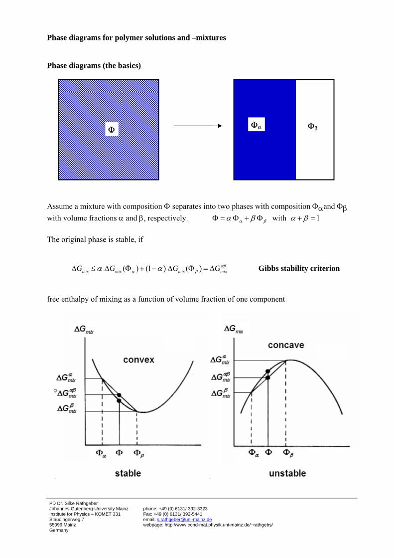
Phase diagrams for polymer solutions and –mixtures Phase diagrams (the basics)
Assume a mixture with composition Φ separates into two phases with composition Φαand Φβ with volume fractions α and β, respectively. with 1α βα β α βΦ = Φ + Φ + = The original phase is stable, if ( ) (1 ) ( )mix mix mix mixG G G Gαβ
α βα αΔ ≤ Δ Φ + − Δ Φ = Δ Gibbs stability criterion free enthalpy of mixing as a function of volume fraction of one component
Φ Φα Φβ
PD Dr. Silke Rathgeber Johannes Gutenberg-University Mainz Institute for Physics – KOMET 331 Staudingerweg 7 55099 Mainz Germany
phone: +49 (0) 6131/ 392-3323 Fax: +49 (0) 6131/ 392-5441 email: [email protected] webpage: http://www.cond-mat.physik.uni-mainz.de/~rathgebs/
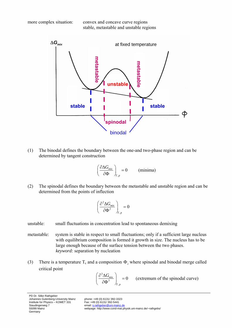
more complex situation: convex and concave curve regions stable, metastable and unstable regions
(1) The binodal defines the boundary between the one-and two-phase region and can be
determined by tangent construction
,
0mix
T p
G∂Δ⎛ ⎞ =⎜ ⎟∂Φ⎝ ⎠ (minima)
(2) The spinodal defines the boundary between the metastable and unstable region and can be
determined from the points of inflection
2
2,
0mix
T p
G⎛ ⎞∂ Δ=⎜ ⎟∂Φ⎝ ⎠
unstable: small fluctuations in concentration lead to spontaneous demixing metastable: system is stable in respect to small fluctuations; only if a sufficient large nucleus with equilibrium composition is formed it growth in size. The nucleus has to be large enough because of the surface tension between the two phases. keyword: separation by nucleation
(3) There is a temperature Tc and a composition cΦ where spinodal and binodal merge called
critical point
3
3,
0mix
T p
G⎛ ⎞∂ Δ=⎜ ⎟∂Φ⎝ ⎠
(extremum of the spinodal curve)
binodal
stable stable
unstable
metastable
metastable
spinodal
mixGΔ at fixed temperature
PD Dr. Silke Rathgeber Johannes Gutenberg-University Mainz Institute for Physics – KOMET 331 Staudingerweg 7 55099 Mainz Germany
phone: +49 (0) 6131/ 392-3323 Fax: +49 (0) 6131/ 392-5441 email: [email protected] webpage: http://www.cond-mat.physik.uni-mainz.de/~rathgebs/
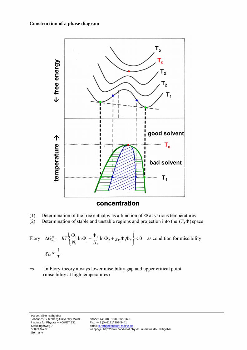
Construction of a phase diagram
(1) Determination of the free enthalpy as a function of Φ at various temperatures (2) Determination of stable and unstable regions and projection into the ( , )T Φ space
Flory 1 21 2 12 1 2
1 2
ln ln 0MmixG RT
N Nχ
⎧ ⎫Φ ΦΔ = Φ + Φ + Φ Φ <⎨ ⎬
⎩ ⎭ as condition for miscibility
121T
χ ∝
⇒ In Flory-theory always lower miscibility gap and upper critical point (miscibility at high temperatures)
free
ene
rgy
tem
pera
ture
concentration
T1
T2
T3
Tc
T5
T1
Tc
good solvent
bad solvent
free
ene
rgy
tem
pera
ture
concentration
T1
T2
T3
Tc
T5
T1
Tc
good solvent
bad solvent
PD Dr. Silke Rathgeber Johannes Gutenberg-University Mainz Institute for Physics – KOMET 331 Staudingerweg 7 55099 Mainz Germany
phone: +49 (0) 6131/ 392-3323 Fax: +49 (0) 6131/ 392-5441 email: [email protected] webpage: http://www.cond-mat.physik.uni-mainz.de/~rathgebs/
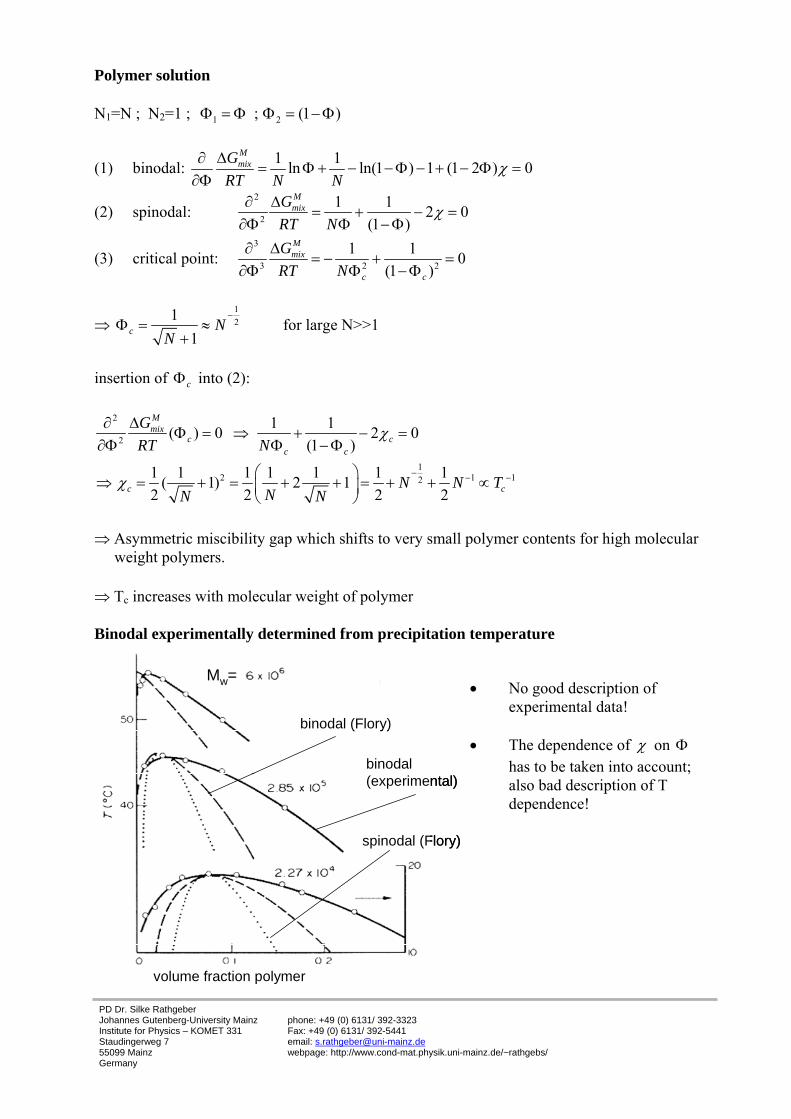
Polymer solution N1=N ; N2=1 ; 1 2; (1 )Φ = Φ Φ = − Φ
(1) binodal: 1 1ln ln(1 ) 1 (1 2 ) 0MmixG
RT N NχΔ∂
= Φ + − − Φ − + − Φ =∂Φ
(2) spinodal: 2
2
1 1 2 0(1 )
MmixG
RT NχΔ∂
= + − =∂Φ Φ − Φ
(3) critical point: 3
3 2 2
1 1 0(1 )
Mmix
c c
GRT N
Δ∂= − + =
∂Φ Φ − Φ
⇒ 121
1c NN
−Φ = ≈
+ for large N>>1
insertion of cΦ into (2):
2
2
12 1 12
1 1( ) 0 2 0(1 )
1 1 1 1 1 1 1( 1) 2 12 2 2 2
Mmix
c cc c
c c
GRT N
N N TNN N
χ
χ− − −
Δ∂Φ = ⇒ + − =
∂Φ Φ − Φ
⎛ ⎞⇒ = + = + + = + + ∝⎜ ⎟⎝ ⎠
⇒ Asymmetric miscibility gap which shifts to very small polymer contents for high molecular weight polymers.
⇒ Tc increases with molecular weight of polymer Binodal experimentally determined from precipitation temperature
• No good description of experimental data!
• The dependence of χ on Φ
has to be taken into account; also bad description of T dependence!
binodal(experimental)
volume fraction polymer
binodal (Flory)
spinodal (Flory)
Mw=
binodal(experimental)
volume fraction polymer
binodal (Flory)
spinodal (Flory)
Mw=
PD Dr. Silke Rathgeber Johannes Gutenberg-University Mainz Institute for Physics – KOMET 331 Staudingerweg 7 55099 Mainz Germany
phone: +49 (0) 6131/ 392-3323 Fax: +49 (0) 6131/ 392-5441 email: [email protected] webpage: http://www.cond-mat.physik.uni-mainz.de/~rathgebs/
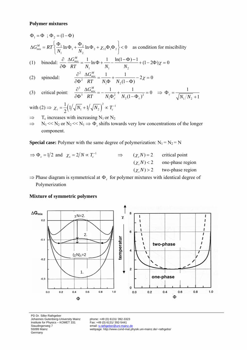
Polymer mixtures
1 2; (1 )Φ = Φ Φ = − Φ
1 21 2 12 1 2
1 2
ln ln 0MmixG RT
N Nχ
⎧ ⎫Φ ΦΔ = Φ + Φ + Φ Φ <⎨ ⎬
⎩ ⎭ as condition for miscibility
(1) binodal: 1 1 2
1 1 ln(1 ) 1ln (1 2 ) 0MmixG
RT N N NχΔ∂ − Φ −
= Φ + − + − Φ =∂Φ
(2) spinodal: 2
21 2
1 1 2 0(1 )
MmixG
RT N NχΔ∂
= + − =∂Φ Φ − Φ
(3) critical point: 3
3 2 21 2 1 2
1 1 10(1 ) 1
Mmix
cc c
GRT N N N N
Δ∂= − + = ⇒ Φ =
∂Φ Φ − Φ +
with (2) ⇒ ( )21
1 21 1 12c cN N Tχ −= + ∝
⇒ Tc increases with increasing N1 or N2 ⇒ N1 << N2 or N2 << N1 ⇒ cΦ shifts towards very low concentrations of the longer
component. Special case: Polymer with the same degree of polymerization: N1 = N2 = N
1c1 2 and 2c cN Tχ −⇒ Φ = = ∝ ⇒ ( ) 2c Nχ = critical point
( ) 2c Nχ < one-phase region ( ) 2c Nχ > two-phase region ⇒ Phase diagram is symmetrical at cΦ for polymer mixtures with identical degree of Polymerization Mixture of symmetric polymers
χ
ΦΦ
χN=2.
(χN)c=2
2.
1.
two-phase
one-phase
ΔGmix
tem
pera
tur
PD Dr. Silke Rathgeber Johannes Gutenberg-University Mainz Institute for Physics – KOMET 331 Staudingerweg 7 55099 Mainz Germany
phone: +49 (0) 6131/ 392-3323 Fax: +49 (0) 6131/ 392-5441 email: [email protected] webpage: http://www.cond-mat.physik.uni-mainz.de/~rathgebs/
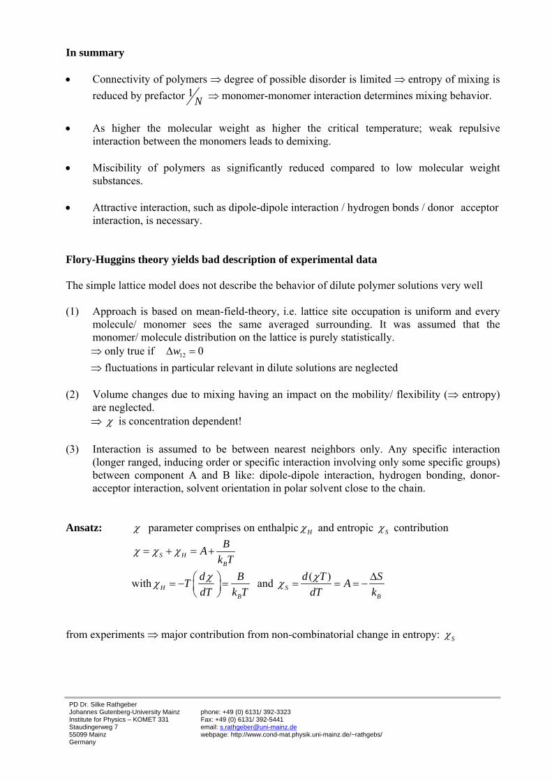
In summary • Connectivity of polymers ⇒ degree of possible disorder is limited ⇒ entropy of mixing is
reduced by prefactor 1N ⇒ monomer-monomer interaction determines mixing behavior.
• As higher the molecular weight as higher the critical temperature; weak repulsive
interaction between the monomers leads to demixing. • Miscibility of polymers as significantly reduced compared to low molecular weight
substances. • Attractive interaction, such as dipole-dipole interaction / hydrogen bonds / donor acceptor
interaction, is necessary. Flory-Huggins theory yields bad description of experimental data The simple lattice model does not describe the behavior of dilute polymer solutions very well (1) Approach is based on mean-field-theory, i.e. lattice site occupation is uniform and every
molecule/ monomer sees the same averaged surrounding. It was assumed that the monomer/ molecule distribution on the lattice is purely statistically. ⇒ only true if 12 0wΔ = ⇒ fluctuations in particular relevant in dilute solutions are neglected
(2) Volume changes due to mixing having an impact on the mobility/ flexibility (⇒ entropy) are neglected. ⇒ χ is concentration dependent!
(3) Interaction is assumed to be between nearest neighbors only. Any specific interaction (longer ranged, inducing order or specific interaction involving only some specific groups) between component A and B like: dipole-dipole interaction, hydrogen bonding, donor-acceptor interaction, solvent orientation in polar solvent close to the chain.
Ansatz: χ parameter comprises on enthalpic Hχ and entropic Sχ contribution
S HB
BAk T
χ χ χ= + = +
with HB
d BTdT k T
χχ ⎛ ⎞= − =⎜ ⎟⎝ ⎠
and ( )S
B
d T SAdT kχχ Δ
= = = −
from experiments ⇒ major contribution from non-combinatorial change in entropy: Sχ
PD Dr. Silke Rathgeber Johannes Gutenberg-University Mainz Institute for Physics – KOMET 331 Staudingerweg 7 55099 Mainz Germany
phone: +49 (0) 6131/ 392-3323 Fax: +49 (0) 6131/ 392-5441 email: [email protected] webpage: http://www.cond-mat.physik.uni-mainz.de/~rathgebs/
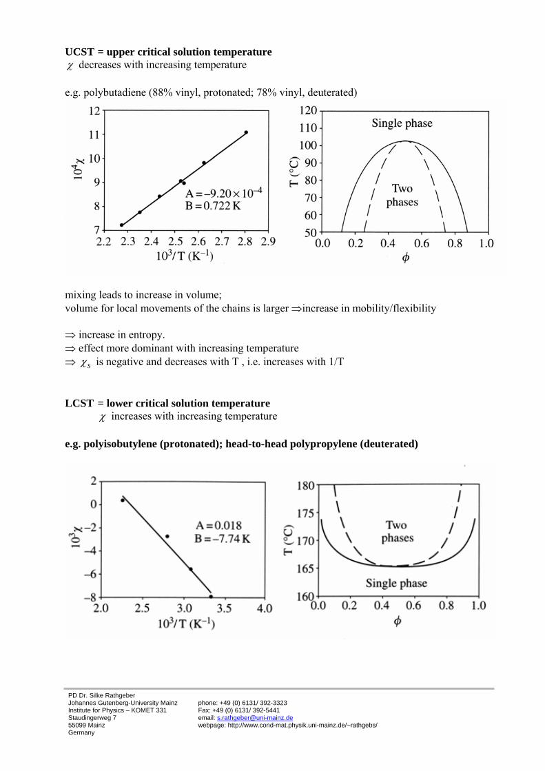
UCST = upper critical solution temperature χ decreases with increasing temperature e.g. polybutadiene (88% vinyl, protonated; 78% vinyl, deuterated)
mixing leads to increase in volume; volume for local movements of the chains is larger ⇒increase in mobility/flexibility ⇒ increase in entropy. ⇒ effect more dominant with increasing temperature ⇒ Sχ is negative and decreases with T , i.e. increases with 1/T LCST = lower critical solution temperature χ increases with increasing temperature e.g. polyisobutylene (protonated); head-to-head polypropylene (deuterated)
PD Dr. Silke Rathgeber Johannes Gutenberg-University Mainz Institute for Physics – KOMET 331 Staudingerweg 7 55099 Mainz Germany
phone: +49 (0) 6131/ 392-3323 Fax: +49 (0) 6131/ 392-5441 email: [email protected] webpage: http://www.cond-mat.physik.uni-mainz.de/~rathgebs/
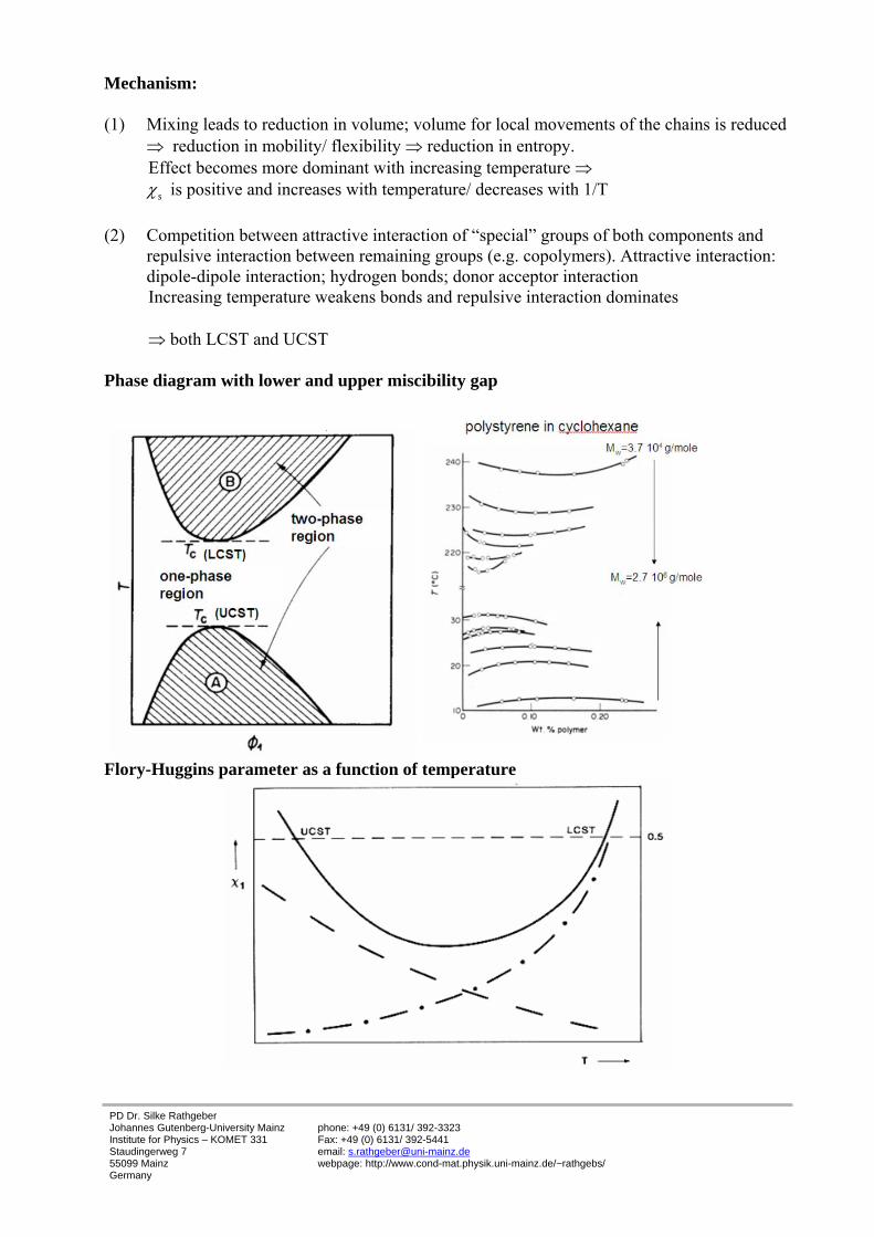
Mechanism: (1) Mixing leads to reduction in volume; volume for local movements of the chains is reduced
⇒ reduction in mobility/ flexibility ⇒ reduction in entropy. Effect becomes more dominant with increasing temperature ⇒ sχ is positive and increases with temperature/ decreases with 1/T (2) Competition between attractive interaction of “special” groups of both components and
repulsive interaction between remaining groups (e.g. copolymers). Attractive interaction: dipole-dipole interaction; hydrogen bonds; donor acceptor interaction
Increasing temperature weakens bonds and repulsive interaction dominates
⇒ both LCST and UCST Phase diagram with lower and upper miscibility gap
Flory-Huggins parameter as a function of temperature
PD Dr. Silke Rathgeber Johannes Gutenberg-University Mainz Institute for Physics – KOMET 331 Staudingerweg 7 55099 Mainz Germany
phone: +49 (0) 6131/ 392-3323 Fax: +49 (0) 6131/ 392-5441 email: [email protected] webpage: http://www.cond-mat.physik.uni-mainz.de/~rathgebs/
4.4 Flory-Krigbaum Theory On the foundation of the excluded volume interactions an enthalpy parameter H and an entropy parameter Ψ for dilution are defined describing deviations from ideal behaviour.
Flory-Huggins: 21ln 1M
d MmixS S p p
S
GG RT c c cn N
μ χ∂Δ ⎡ ⎤⎛ ⎞Δ = = Δ = + − +⎜ ⎟⎢ ⎥∂ ⎝ ⎠⎣ ⎦
with cp << 1 21ln ln(1 ) ...2S p p pc c c c⇒ = − ≈ − − + as for osmotic pressure
2
deviations from ideal behavior
1[ ...]2
pd MS p
cG RT c
Nμ χ⎛ ⎞⇒ Δ = Δ = − + − +⎜ ⎟
⎝ ⎠14243
Flory-Krigbaum: dilution enthalpy: 2d
ni pH RTHcΔ =
dilution entropy: 2dni pS R cΔ = Ψ ( 2
pc due to pair contacts) ⇒ free enthalpy of dilution: 2( )d
ni pG RT H cΔ = − Ψ
⇒ comparison Flory-Huggins and Flory-Krigbaum theory: 1( )2
H χ⎛ ⎞− − Ψ = −⎜ ⎟⎝ ⎠
θ conditions: 12
Hχ = ⇔ = Ψ ; i.e. d dni niH T SΔ = Δ
define: HTθ =Ψ
(only defined if H and Ψ have equal sign)
non-ideal behavior disappears for T θ= !
replace 1 12 T
θχ ⎛ ⎞− = Ψ − =⎜ ⎟⎝ ⎠
2nd virial coefficient A2 !
21 ...pd MS p
cG RT c
N Tθμ
⎡ ⎤⎛ ⎞⇒ Δ = Δ = − + Ψ − +⎜ ⎟⎢ ⎥⎝ ⎠⎣ ⎦
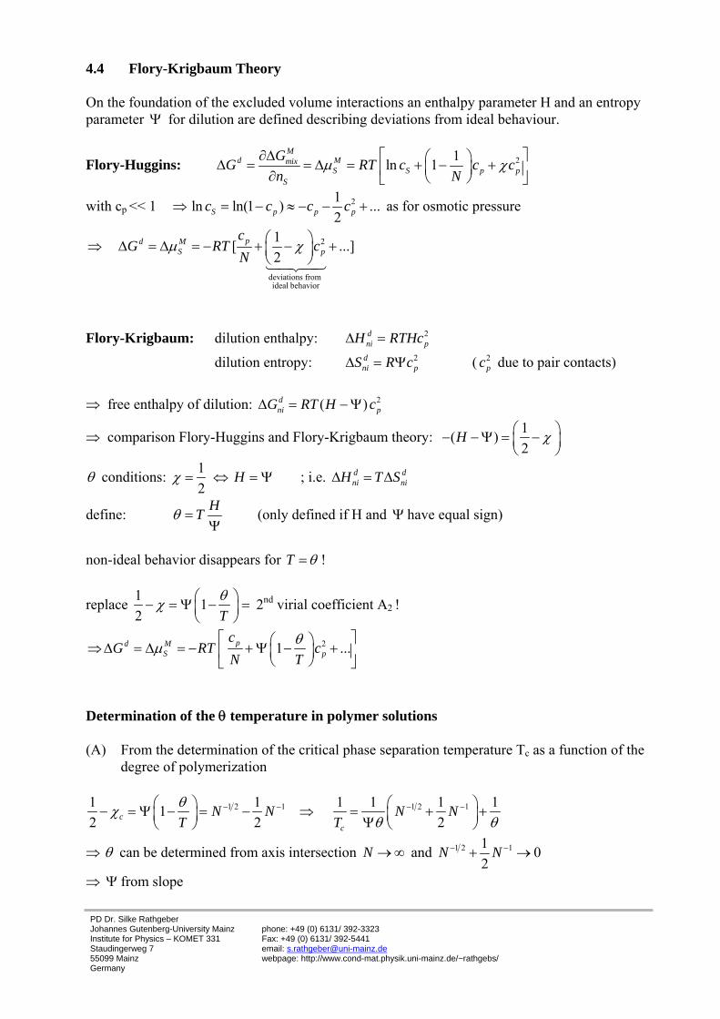
Determination of the θ temperature in polymer solutions (A) From the determination of the critical phase separation temperature Tc as a function of the
degree of polymerization
1 2 1 1 2 11 1 1 1 1 112 2 2c
c
N N N NT Tθχ
θ θ− − − −⎛ ⎞ ⎛ ⎞− = Ψ − = − ⇒ = + +⎜ ⎟ ⎜ ⎟Ψ⎝ ⎠ ⎝ ⎠
⇒ θ can be determined from axis intersection N → ∞ and 1 2 11 02
N N− −+ →
⇒ Ψ from slope
PD Dr. Silke Rathgeber Johannes Gutenberg-University Mainz Institute for Physics – KOMET 331 Staudingerweg 7 55099 Mainz Germany
phone: +49 (0) 6131/ 392-3323 Fax: +49 (0) 6131/ 392-5441 email: [email protected] webpage: http://www.cond-mat.physik.uni-mainz.de/~rathgebs/
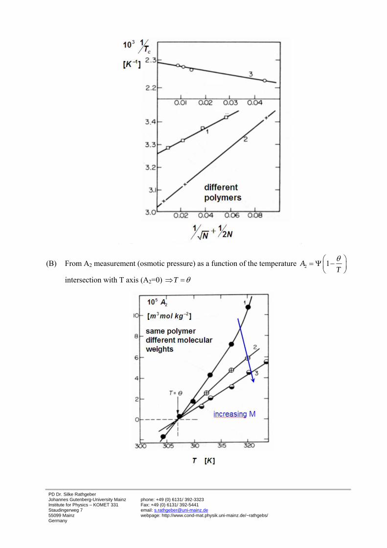
(B) From A2 measurement (osmotic pressure) as a function of the temperature 2 1ATθ⎛ ⎞= Ψ −⎜ ⎟
⎝ ⎠
intersection with T axis (A2=0) T θ⇒ =
PD Dr. Silke Rathgeber Johannes Gutenberg-University Mainz Institute for Physics – KOMET 331 Staudingerweg 7 55099 Mainz Germany
phone: +49 (0) 6131/ 392-3323 Fax: +49 (0) 6131/ 392-5441 email: [email protected] webpage: http://www.cond-mat.physik.uni-mainz.de/~rathgebs/
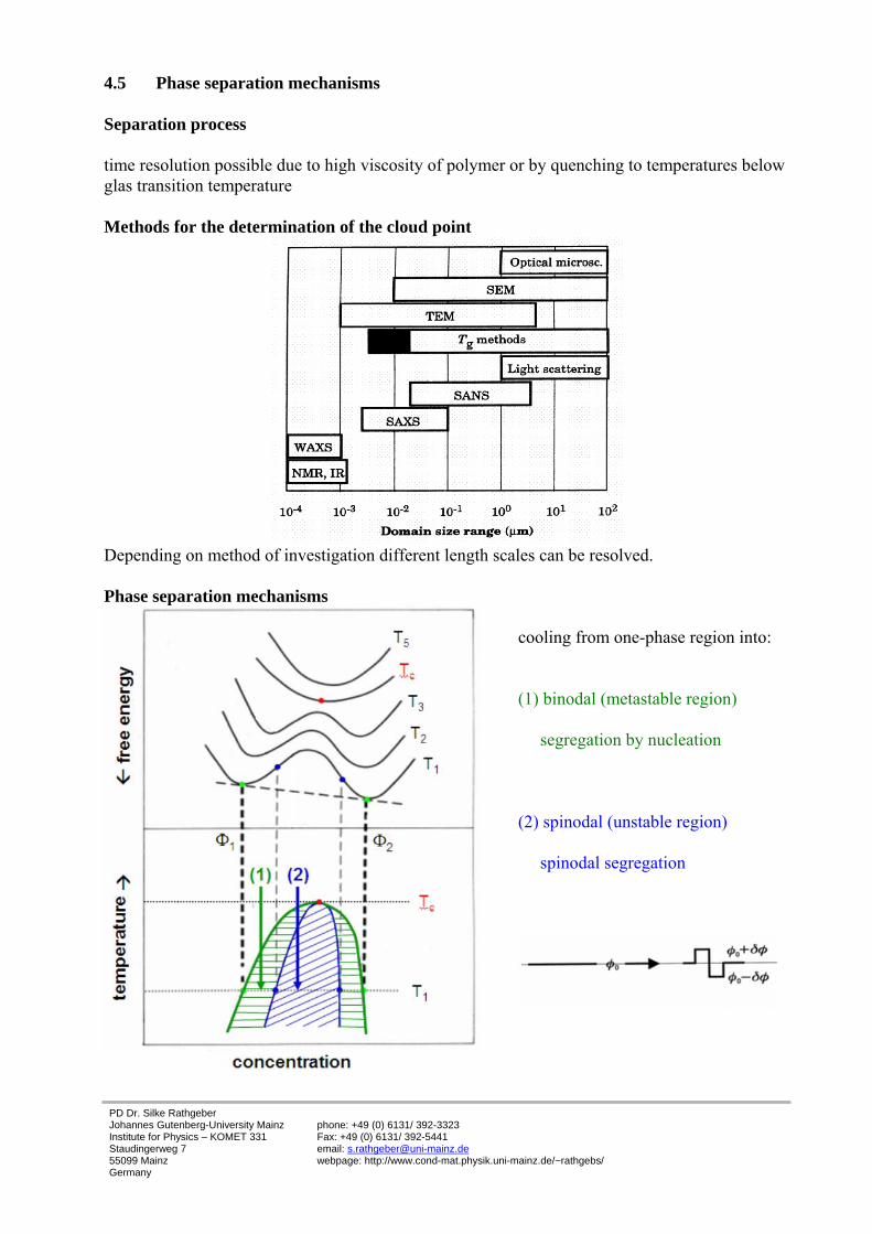
4.5 Phase separation mechanisms Separation process time resolution possible due to high viscosity of polymer or by quenching to temperatures below glas transition temperature Methods for the determination of the cloud point
Depending on method of investigation different length scales can be resolved. Phase separation mechanisms
cooling from one-phase region into: (1) binodal (metastable region) segregation by nucleation (2) spinodal (unstable region) spinodal segregation
PD Dr. Silke Rathgeber Johannes Gutenberg-University Mainz Institute for Physics – KOMET 331 Staudingerweg 7 55099 Mainz Germany
phone: +49 (0) 6131/ 392-3323 Fax: +49 (0) 6131/ 392-5441 email: [email protected] webpage: http://www.cond-mat.physik.uni-mainz.de/~rathgebs/
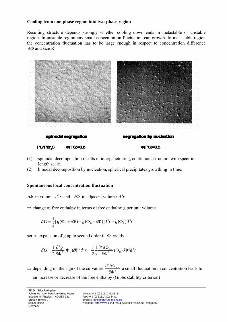
Cooling from one-phase region into two-phase region Resulting structure depends strongly whether cooling down ends in metastable or unstable region. In unstable region any small concentration fluctuation can growth. In metastable region the concentration fluctuation has to be large enough in respect to concentration difference ΔΦ and size R
(1) spinodal decomposition results in interpenetrating, continuous structure with specific
length scale. (2) binodal decomposition by nucleation, spherical precipitates growthing in time.
Spontaneous local concentration fluctuation δΦ in volume 3d r and δ− Φ in adjacent volume 3d r ⇒ change of free enthalpy in terms of free enthalpy g per unit volume
3 30 0 0
1 [ ( ) ( )] ( )2
G g g d r g d rδ δ δ= Φ + Φ + Φ − Φ − Φ
series expansion of g up to second order in Φ yields
22
2 3 2 30 02 2
1 1 1( ) ( )2 2
mixGgG d r d rv
δ δ δ∂ Δ∂= Φ Φ = Φ Φ
∂Φ ∂Φ
⇒ depending on the sign of the curvature 2
2mixG∂ Δ
∂Φ a small fluctuation in concentration leads to
an increase or decrease of the free enthalpy (Gibbs stability criterion)
PD Dr. Silke Rathgeber Johannes Gutenberg-University Mainz Institute for Physics – KOMET 331 Staudingerweg 7 55099 Mainz Germany
phone: +49 (0) 6131/ 392-3323 Fax: +49 (0) 6131/ 392-5441 email: [email protected] webpage: http://www.cond-mat.physik.uni-mainz.de/~rathgebs/
(1) 2
2 0 (convex) 0mixG Gδ⎛ ⎞∂ Δ
> >⎜ ⎟∂Φ⎝ ⎠ phase is stable against small pertubation;
amplitude of small pertubation decays
(2) 2
2 0 (concave) 0mixG Gδ⎛ ⎞∂ Δ
< <⎜ ⎟∂Φ⎝ ⎠ phase is unstable against small pertubation;
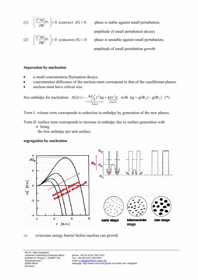
amplitude of small pertubation growth Separation by nucleation • a small concentration fluctuation decays. • concentration difference of the nucleus must correspond to that of the equilibrium phases. • nucleus must have critical size. free enthalpy for nucleation: 3 2
0 2Term II
Term I
4( ) 4 with ( ) ( )3G r r g r g g gπ π σΔ = − Δ + Δ = Φ − Φ12314243
(*)
Term I: volume term corresponds to reduction in enthalpy by generation of the new phases. Term II: surface term corresponds to increase in enthalpy due to surface generation with σ being the free enthalpy per unit surface. segregation by nucleation
⇒ overcome energy barrier before nucleus can growth
PD Dr. Silke Rathgeber Johannes Gutenberg-University Mainz Institute for Physics – KOMET 331 Staudingerweg 7 55099 Mainz Germany
phone: +49 (0) 6131/ 392-3323 Fax: +49 (0) 6131/ 392-5441 email: [email protected] webpage: http://www.cond-mat.physik.uni-mainz.de/~rathgebs/
⇒ nucleation rate increases with Arrhenius law: exp bnucleus
B
Gk T
ν⎛ ⎞Δ
∝ −⎜ ⎟⎝ ⎠
with the barrier height 3
2
163 ( )bG
gπ σ
Δ =Δ
which is the maximum of (*) ( )G rΔ
⇒ energy barrier bGΔ increases with decreasing distance from the binodal (approaching from spinodal); at the binodal 0gΔ = bG⇒ Δ → ∞ ⇒ mixture needs to be supercooled (or overheated) to achieve relevant nucleation rates. In summary • nucleus growth diffusion controlled; downhill-diffusion towards decreasing concentrations
(chemical potential gradient supports feeding nucleus). • decreasing temperature ⇒ diffusion slower (nucleus growth slower); nucleation rate
increases (for lower miscibility gap) ⇒ number of nuclei increases • droplet size, number and distance depend on time and temperature • at later stages coalescence, coarsening and ripening until there are two large phases with
composition 1Φ and 2Φ Spinodal Decomposition
• at spinodal 2
2 0mixG∂ Δ→ ⇒
∂Φspontaneous demixing; no activation energy
• no sharp transition from phase separation by nucleation to spontaneous demixing since 2
2mixG∂ Δ
∂Φ vanishes continuously
Kinetics of spinodal decomposition in polymer mixtures • local chemical potential difference caused by concentration fluctuations
0
Term IITerm I
2mixs s
Gμ μ μ κ 2∂ΔΔ = − = − ∇ Φ
∂Φ 14243123
Term I: homogenous system Term II: gradient energy term associated with departure from uniformity κ = gradient energy coefficient (empirical constant) • difference in the chemical potentials causes interdiffusion flux. Linear response between flux
and gradient in chemical potential:
PD Dr. Silke Rathgeber Johannes Gutenberg-University Mainz Institute for Physics – KOMET 331 Staudingerweg 7 55099 Mainz Germany
phone: +49 (0) 6131/ 392-3323 Fax: +49 (0) 6131/ 392-5441 email: [email protected] webpage: http://www.cond-mat.physik.uni-mainz.de/~rathgebs/
2
32( ) 2mixGj μ κ
⎡ ⎤∂ Δ− = Ω∇ Δ = Ω ∇Φ − ∇ Φ⎢ ⎥∂Φ⎣ ⎦
with Ω =Onsager-type phenomenological coefficient • substitution into equation of continuity which equates the net flux over a surface with the
loss
or gain of material within the surface 2
2 42 2mixGj
tκ
⎡ ⎤∂ Δ∂Φ= −∇ ⋅ = Ω ∇ Φ − ∇ Φ⎢ ⎥∂ ∂Φ⎣ ⎦
Cahn-Hillard relation • comparison to conventional diffusion equation
2Dt
∂Φ= ∇ Φ
∂ (D=diffusion coefficient)
2
2 0mixGD ∂ Δ⇒ ≈ Ω <
∂Φ in unstable region
diffusion against concentration gradient at spinodal ( )SpT T→ 0D → “critical slowing down” general solution for Cahn-Hilliard relation: 0 exp( ( ) ) [ ( ) cos( ) ( )sin( )]t A x B x
β
β β β β βΦ − Φ = Γ ⋅ ⋅ +∑
with 2πλβ
= and {
22 2
20
( ) 2mixGβ β κβ>
⎡ ⎤∂ ΔΓ = −Ω −⎢ ⎥
∂Φ⎢ ⎥⎣ ⎦
stable region: 2
2 0 ( ) 0mixG β∂ Δ> ⇒ Γ < ⇒
∂Φ instabilities rapidly decay
unstable region: 2
2 0 ( ) 0mixG β∂ Δ< ⇒ Γ > ⇒
∂Φ some wavelengths notably the long
wavelengths (small β ) will grow
PD Dr. Silke Rathgeber Johannes Gutenberg-University Mainz Institute for Physics – KOMET 331 Staudingerweg 7 55099 Mainz Germany
phone: +49 (0) 6131/ 392-3323 Fax: +49 (0) 6131/ 392-5441 email: [email protected] webpage: http://www.cond-mat.physik.uni-mainz.de/~rathgebs/
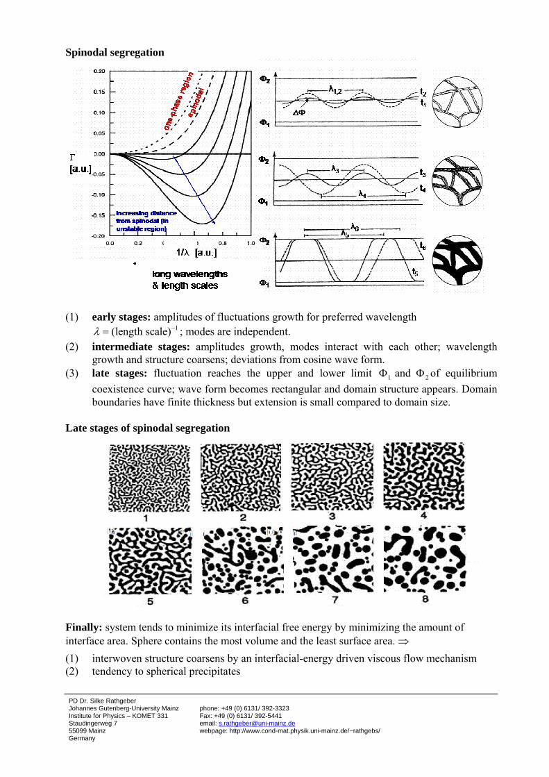
Spinodal segregation
(1) early stages: amplitudes of fluctuations growth for preferred wavelength
1(length scale)λ −= ; modes are independent. (2) intermediate stages: amplitudes growth, modes interact with each other; wavelength
growth and structure coarsens; deviations from cosine wave form. (3) late stages: fluctuation reaches the upper and lower limit 1 2and Φ Φ of equilibrium
coexistence curve; wave form becomes rectangular and domain structure appears. Domain boundaries have finite thickness but extension is small compared to domain size.
Late stages of spinodal segregation
Finally: system tends to minimize its interfacial free energy by minimizing the amount of interface area. Sphere contains the most volume and the least surface area. ⇒
(1) interwoven structure coarsens by an interfacial-energy driven viscous flow mechanism (2) tendency to spherical precipitates
PD Dr. Silke Rathgeber Johannes Gutenberg-University Mainz Institute for Physics – KOMET 331 Staudingerweg 7 55099 Mainz Germany
phone: +49 (0) 6131/ 392-3323 Fax: +49 (0) 6131/ 392-5441 email: [email protected] webpage: http://www.cond-mat.physik.uni-mainz.de/~rathgebs/
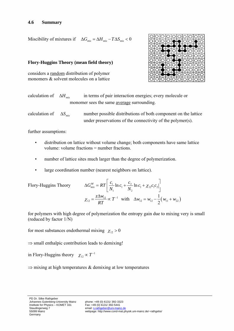
4.6 Summary Miscibility of mixtures if 0mix mix mixG H T SΔ = Δ − Δ < Flory-Huggins Theory (mean field theory) considers a random distribution of polymer monomers & solvent molecules on a lattice calculation of mixHΔ in terms of pair interaction energies; every molecule or monomer sees the same average surrounding. calculation of mixSΔ number possible distributions of both component on the lattice under preservations of the connectivity of the polymer(s). further assumptions:
• distribution on lattice without volume change; both components have same lattice volume: volume fractions = number fractions.
• number of lattice sites much larger than the degree of polymerization.
• large coordination number (nearest neighbors on lattice).
Flory-Huggins Theory 1 21 1 12 1 2
1 2
ln lnMmix
c cG RT c c c cN N
χ⎡ ⎤
Δ = + +⎢ ⎥⎣ ⎦
11212
z w TRT
χ −Δ= ∝ with ( )12 12 11 22
12
w w w wΔ = − +
for polymers with high degree of polymerization the entropy gain due to mixing very is small (reduced by factor 1/N) for most substances endothermal mixing 12 0>χ ⇒ small enthalpic contribution leads to demixing! in Flory-Huggins theory 1
12−∝ Tχ
⇒ mixing at high temperatures & demixing at low temperatures
PD Dr. Silke Rathgeber Johannes Gutenberg-University Mainz Institute for Physics – KOMET 331 Staudingerweg 7 55099 Mainz Germany
phone: +49 (0) 6131/ 392-3323 Fax: +49 (0) 6131/ 392-5441 email: [email protected] webpage: http://www.cond-mat.physik.uni-mainz.de/~rathgebs/
Osmotic pressure is the pressure produced by a solution in a space that is enclosed by a semi-permeable membrane. Π = pressure polymer solution – pressure pure solvent
21( ) ...2
Ps P
cV RT cN
χ⎡ ⎤Π = + − +⎢ ⎥⎣ ⎦
12
χ < good solvent - high temperatures - polymer swells
12
χ > bad solvent - low temperatures - polymer shrinks
12
χ = θ solvent
Membrane osmometry (measures excess column height) hydrostatic pressure = osmotic pressure dilute solutions:
1 1( ) ...2
sP
P
V cRTc N
χΠ ⎡ ⎤= + − +⎢ ⎥⎣ ⎦
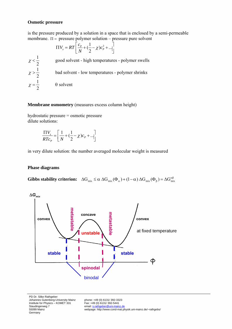
in very dilute solution: the number averaged molecular weight is measured Phase diagrams Gibbs stability criterion: mix mix mix mixG G ( ) (1 ) G ( ) Gαβ
α βΔ ≤ α Δ Φ + − α Δ Φ = Δ
stable stable
unstable
metastable
metastable
spinodal
binodal
mixGΔ
at fixed temperature
convexconvex concave
PD Dr. Silke Rathgeber Johannes Gutenberg-University Mainz Institute for Physics – KOMET 331 Staudingerweg 7 55099 Mainz Germany
phone: +49 (0) 6131/ 392-3323 Fax: +49 (0) 6131/ 392-5441 email: [email protected] webpage: http://www.cond-mat.physik.uni-mainz.de/~rathgebs/
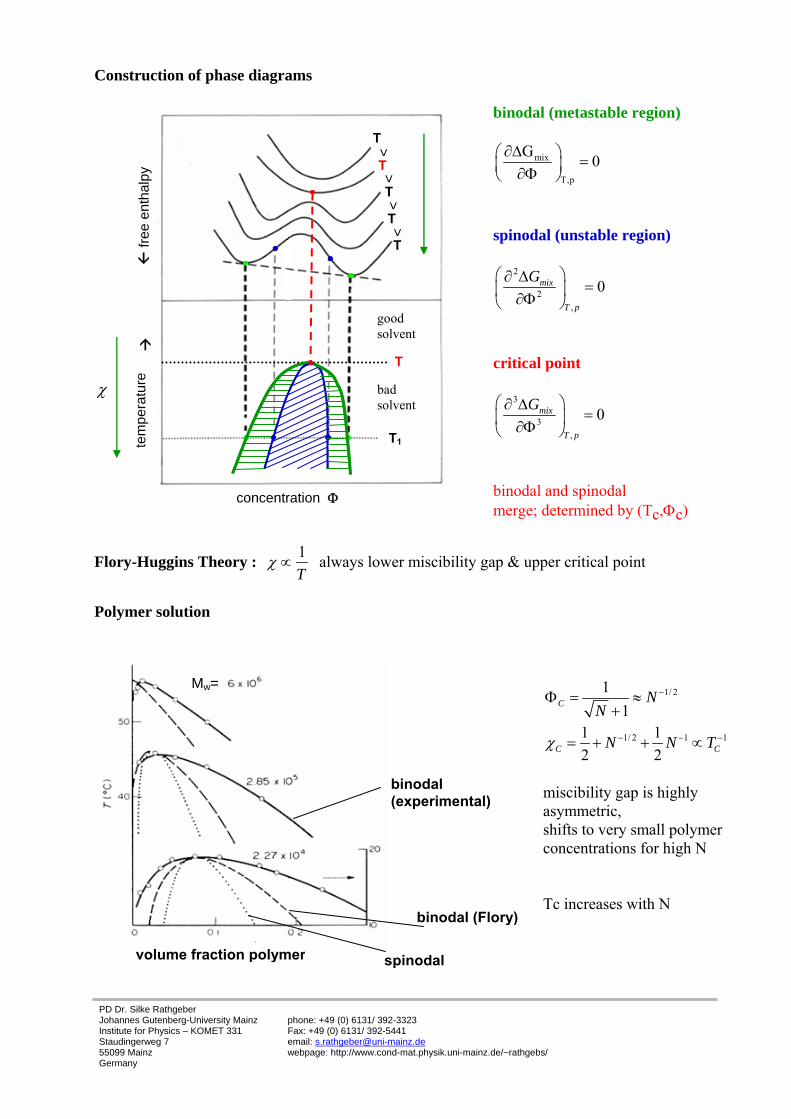
Construction of phase diagrams
binodal (metastable region)
mix
T,p
G 0∂Δ⎛ ⎞ =⎜ ⎟∂Φ⎝ ⎠
spinodal (unstable region)
2
2,
0⎛ ⎞∂ Δ
=⎜ ⎟∂Φ⎝ ⎠mix
T p
G
critical point
3
3,
0⎛ ⎞∂ Δ
=⎜ ⎟∂Φ⎝ ⎠mix
T p
G
binodal and spinodal merge; determined by (Tc,Φc)
Flory-Huggins Theory : 1T
χ ∝ always lower miscibility gap & upper critical point
Polymer solution
1/ 2
1/ 2 1 1
11
1 12 2
C
C C
NN
N N Tχ
−
− − −
Φ = ≈+
= + + ∝
miscibility gap is highly asymmetric, shifts to very small polymer concentrations for high N Tc increases with N
binodal (experimental)
volume fraction polymer
binodal (Flory)
spinodal
Mw=
free
ent
halp
y
tem
pera
ture
concentration Φ
T
T
T
T
T
T1
T
> >
> >
χ
good solvent
bad solvent
PD Dr. Silke Rathgeber Johannes Gutenberg-University Mainz Institute for Physics – KOMET 331 Staudingerweg 7 55099 Mainz Germany
phone: +49 (0) 6131/ 392-3323 Fax: +49 (0) 6131/ 392-5441 email: [email protected] webpage: http://www.cond-mat.physik.uni-mainz.de/~rathgebs/
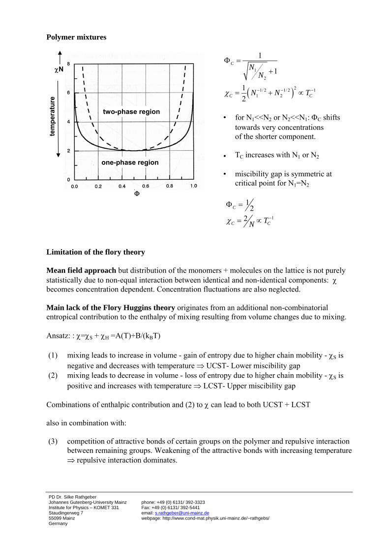
Polymer mixtures
( )
1
2
21/ 2 1/ 2 11 2
1
1
12
− − −
Φ =+
= + ∝
C
C C
NN
N N Tχ
• for N1<<N2 or N2<<N1: ΦC shifts
towards very concentrations of the shorter component.
• TC increases with N1 or N2
• miscibility gap is symmetric at critical point for N1=N2
1
12
2 −
Φ =
= ∝
C
C CTNχ
Limitation of the flory theory Mean field approach but distribution of the monomers + molecules on the lattice is not purely statistically due to non-equal interaction between identical and non-identical components: χ becomes concentration dependent. Concentration fluctuations are also neglected. Main lack of the Flory Huggins theory originates from an additional non-combinatorial entropical contribution to the enthalpy of mixing resulting from volume changes due to mixing. Ansatz: : χ=χS + χH =A(T)+B/(kBT) (1) mixing leads to increase in volume - gain of entropy due to higher chain mobility - χS is
negative and decreases with temperature ⇒ UCST- Lower miscibility gap (2) mixing leads to decrease in volume - loss of entropy due to higher chain mobility - χS is
positive and increases with temperature ⇒ LCST- Upper miscibility gap Combinations of enthalpic contribution and (2) to χ can lead to both UCST + LCST also in combination with: (3) competition of attractive bonds of certain groups on the polymer and repulsive interaction
between remaining groups. Weakening of the attractive bonds with increasing temperature ⇒ repulsive interaction dominates.
χN
Φ
two-phase region
one-phase region
tem
pera
ture
PD Dr. Silke Rathgeber Johannes Gutenberg-University Mainz Institute for Physics – KOMET 331 Staudingerweg 7 55099 Mainz Germany
phone: +49 (0) 6131/ 392-3323 Fax: +49 (0) 6131/ 392-5441 email: [email protected] webpage: http://www.cond-mat.physik.uni-mainz.de/~rathgebs/
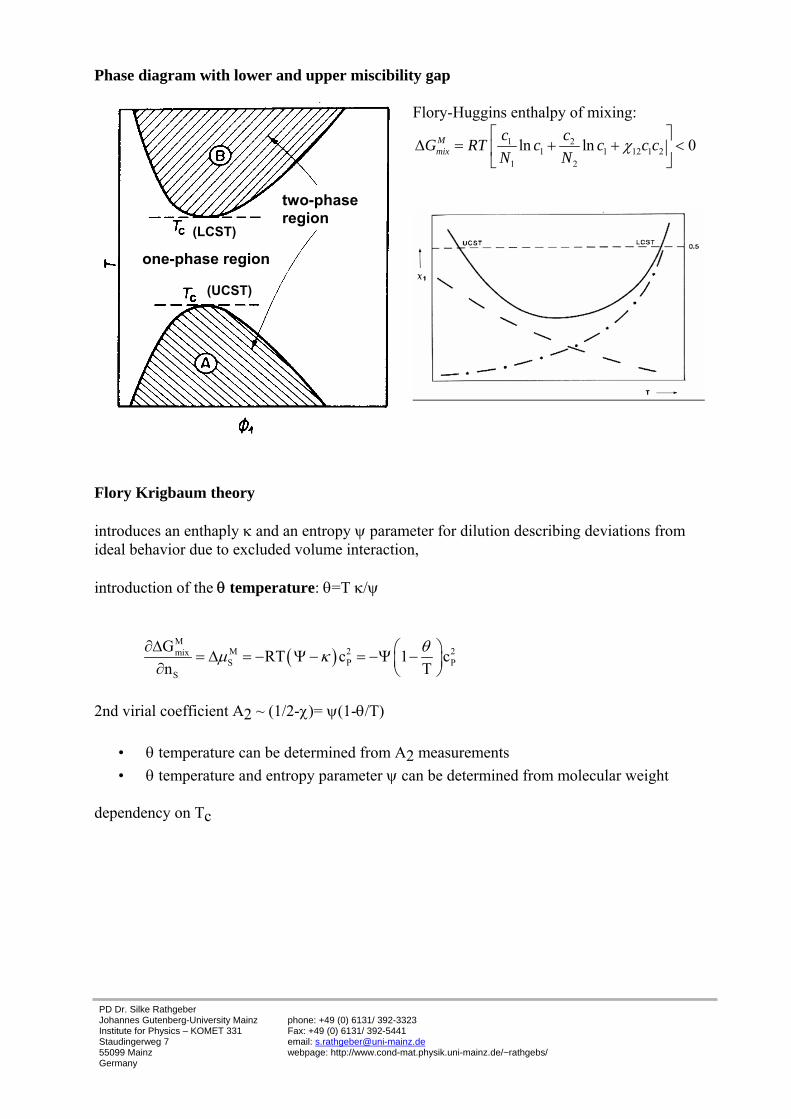
Phase diagram with lower and upper miscibility gap
Flory-Huggins enthalpy of mixing:
1 21 1 12 1 2
1 2
ln ln 0⎡ ⎤
Δ = + + <⎢ ⎥⎣ ⎦
Mmix
c cG RT c c c cN N
χ
Flory Krigbaum theory introduces an enthaply κ and an entropy ψ parameter for dilution describing deviations from ideal behavior due to excluded volume interaction, introduction of the θ temperature: θ=T κ/ψ
( )M
M 2 2mixS P P
S
G RT c 1 cn T
∂Δ ⎛ ⎞= Δ = − Ψ − = −Ψ −⎜ ⎟∂ ⎝ ⎠θμ κ
2nd virial coefficient A2 ~ (1/2-χ)= ψ(1-θ/T)
• θ temperature can be determined from A2 measurements • θ temperature and entropy parameter ψ can be determined from molecular weight
dependency on Tc
one-phase region
two-phase region
(UCST)
(LCST)
PD Dr. Silke Rathgeber Johannes Gutenberg-University Mainz Institute for Physics – KOMET 331 Staudingerweg 7 55099 Mainz Germany
phone: +49 (0) 6131/ 392-3323 Fax: +49 (0) 6131/ 392-5441 email: [email protected] webpage: http://www.cond-mat.physik.uni-mainz.de/~rathgebs/
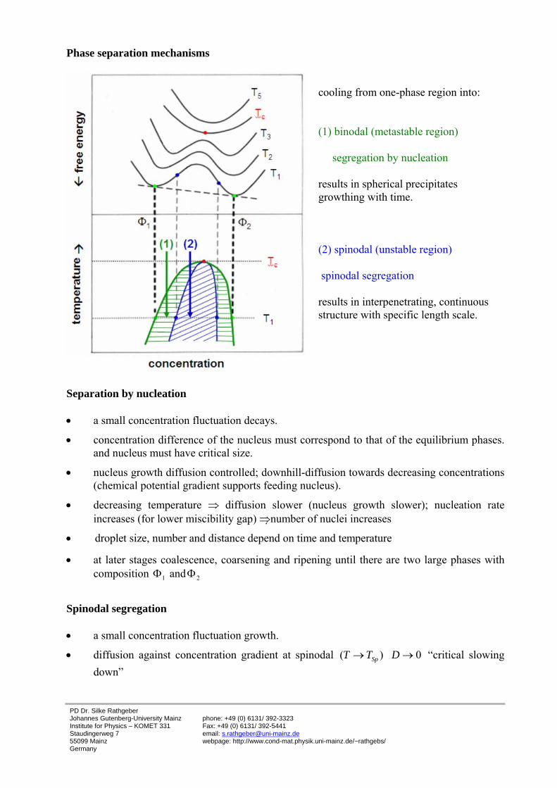
Phase separation mechanisms
cooling from one-phase region into: (1) binodal (metastable region) segregation by nucleation results in spherical precipitates growthing with time. (2) spinodal (unstable region) spinodal segregation results in interpenetrating, continuous structure with specific length scale.
Separation by nucleation • a small concentration fluctuation decays.
• concentration difference of the nucleus must correspond to that of the equilibrium phases. and nucleus must have critical size.
• nucleus growth diffusion controlled; downhill-diffusion towards decreasing concentrations (chemical potential gradient supports feeding nucleus).
• decreasing temperature ⇒ diffusion slower (nucleus growth slower); nucleation rate increases (for lower miscibility gap) ⇒number of nuclei increases
• droplet size, number and distance depend on time and temperature
• at later stages coalescence, coarsening and ripening until there are two large phases with composition 1Φ and 2Φ
Spinodal segregation • a small concentration fluctuation growth.
• diffusion against concentration gradient at spinodal ( )SpT T→ 0D → “critical slowing down”
PD Dr. Silke Rathgeber Johannes Gutenberg-University Mainz Institute for Physics – KOMET 331 Staudingerweg 7 55099 Mainz Germany
phone: +49 (0) 6131/ 392-3323 Fax: +49 (0) 6131/ 392-5441 email: [email protected] webpage: http://www.cond-mat.physik.uni-mainz.de/~rathgebs/
Stages
(1) early stages: amplitudes of fluctuations growth for preferred wavelength
1(length scale)λ −= ; modes are independent.
(2) intermediate stages: amplitudes growth, modes interact with each other; wavelength growth and structure coarsens; deviations from cosine wave form.
(3) late stages: fluctuation reaches the upper and lower limit 1 2and Φ Φ of equilibrium coexistence curve; wave form becomes rectangular and domain structure appears. Domain boundaries have finite thickness but extension is small compared to domain size.
(4) Finally: system tends to minimize its interfacial free energy by minimizing the amount of interface area. Sphere contains the most volume and the least surface area. ⇒ • interwoven structure coarsens by an interfacial-energy driven viscous flow mechanism • tendency to spherical precipitates
PD Dr. Silke Rathgeber Johannes Gutenberg-University Mainz Institute for Physics – KOMET 331 Staudingerweg 7 55099 Mainz Germany
phone: +49 (0) 6131/ 392-3323 Fax: +49 (0) 6131/ 392-5441 email: [email protected] webpage: http://www.cond-mat.physik.uni-mainz.de/~rathgebs/
Literature 1. U.W. Gedde, “Polymer Physics”, Chapman & Hall, London, 1995. 2. G. Strobl, “The Physics of Polymers”, Springer-Verlag, Berlin, 1996. 3. M.D. Lechner, K. Gehrke, E.H. Nordmeier, “ Makromolekulare Chemie”, Birkhäuser
Verlag, Basel, 1993. 4. J.M.G. Cowie, “Polymers: Chemistry & Physics of Modern Materials”, Blackie Academic
& Professional, London, 1991. 5. K. Kamide, T. Dobashi, “Physical Chemistry of Polymer Solutions”, Elsevier, Amsterdam,
2000. 6. O. Olabisi, L.M. Robeson, M.T. Shaw, “Polymer-Polymer Miscibility”, Academic Press,
San Diego, 1997. 7. M. Rubinstein, R.H. Colby, “Polymer Physics“, Oxford University Press, New York, 2003. 8. U, Eisele, “Introduction to Polymer Physics”, Springer Verlag, Berlin. 1990. 9. M. Doi, “Introduction to Polymer Physics”, Chapman & Hill, London, 1995. 10. A. Baumgärtner, “ Polymer Mixtures”, Lecture Manuscripts of the 33th IFF Winter School
on “ Soft Matter – Complex Materials on Mesoscopic Scales”, 2002. 11. T. Springer, “ Entmischungskinetik bei Polymeren”, Lecture Manuscripts of the 28th IFF
Winter School on “ Dynamik und Strukturbildung in kondensierter Materie”, 1997. 12. K. Kehr, “ Mittlere Feld-Theorie der Polymerlösungen, Schmelzen und Mischungen;
Random Phase Approximation”, Lecture Manuscripts of the 22th IFF Winter School on “ Physik der Polymere”, 1991.
13. H. Müller-Krumbhaar, “ Entmischungskinetik eines Polymer-Gemisches”, Lecture Manuscripts of the 22th IFF Winter School on “ Physik der Polymere”, 1991.
14. T. Springer, “ Dichte Polymersysteme und Lösungen”, Lecture Manuscripts of the 25th IFF Winter School on “ Komplexe Systeme zwischen Atom und Festkörper”, 1994.
15. H. Müller-Krumbhaar, “ Phasenübergange: Ordnung und Fluktuationen ”, Lecture Manuscripts of the 25th IFF Winter School on “ Komplexe Systeme zwischen Atom und Festkörper”, 1994.