Johann Wolfgang Goethe University, Frankfurt am Main · Johann Wolfgang Goethe University,...

arX

iv:1

010.

0161

v1 [

mat

h.PR

] 1

Oct

201

0

The Annals of Probability

2010, Vol. 38, No. 2, 532–569DOI: 10.1214/09-AOP500c© Institute of Mathematical Statistics, 2010

TAYLOR EXPANSIONS OF SOLUTIONS OF STOCHASTIC

PARTIAL DIFFERENTIAL EQUATIONS WITH ADDITIVE NOISE1

By Arnulf Jentzen and Peter Kloeden

Johann Wolfgang Goethe University, Frankfurt am Main

The solution of a parabolic stochastic partial differential equation(SPDE) driven by an infinite-dimensional Brownian motion is in gen-eral not a semi-martingale anymore and does in general not satisfyan Ito formula like the solution of a finite-dimensional stochastic or-dinary differential equation (SODE). In particular, it is not possibleto derive stochastic Taylor expansions as for the solution of a SODEusing an iterated application of the Ito formula. Consequently, un-til recently, only low order numerical approximation results for sucha SPDE have been available. Here, the fact that the solution of aSPDE driven by additive noise can be interpreted in the mild sensewith integrals involving the exponential of the dominant linear op-erator in the SPDE provides an alternative approach for derivingstochastic Taylor expansions for the solution of such a SPDE. Es-sentially, the exponential factor has a mollifying effect and ensuresthat all integrals take values in the Hilbert space under consideration.The iteration of such integrals allows us to derive stochastic Taylorexpansions of arbitrarily high order, which are robust in the sensethat they also hold for other types of driving noise processes suchas fractional Brownian motion. Combinatorial concepts of trees andwoods provide a compact formulation of the Taylor expansions.

1. Introduction. Taylor expansions are a fundamental and repeatedlyused method of approximation in mathematics, in particular in numeri-cal analysis. Although numerical schemes for ordinary differential equations(ODEs) are often derived in an ad hoc manner, those based on Taylor ex-pansions of the solution of an ODE, the Taylor schemes, provide a class ofschemes with known convergence orders against which other schemes can be

Received September 2008; revised July 2009.1Supported by the DFG project “Pathwise numerics and dynamics of stochastic evo-

lution equations.”AMS 2000 subject classifications. 35K90, 41A58, 65C30, 65M99.Key words and phrases. Taylor expansions, stochastic partial differential equations,

SPDE, strong convergence, stochastic trees.

This is an electronic reprint of the original article published by theInstitute of Mathematical Statistics in The Annals of Probability,2010, Vol. 38, No. 2, 532–569. This reprint differs from the original in paginationand typographic detail.

1

http://arxiv.org/abs/1010.0161v1

http://www.imstat.org/aop/

http://dx.doi.org/10.1214/09-AOP500

http://www.imstat.org

http://www.ams.org/msc/

http://www.imstat.org

http://www.imstat.org/aop/

http://dx.doi.org/10.1214/09-AOP500

2 A. JENTZEN AND P. KLOEDEN

compared to determine their order. An important component of such Taylorschemes are the iterated total derivatives of the vector field correspondinghigher derivatives of the solution, which are obtained via the chain rule; see[8].

An analogous situation holds for Ito stochastic ordinary differential equa-tions (SODEs), except, due to the less robust nature of stochastic calculus,stochastic Taylor schemes instead of classical Taylor schemes are the start-ing point to obtain consistent higher order numerical schemes, see [29] forthe general theory. Another important difference is that SODEs are reallyjust a symbolic representation of stochastic integral equations since theirsolutions are not differentiable, so an integral version of Taylor expansionsbased on iterated application of the stochastic chain rule, the Ito formula,is required. Underlying this method is the fact that the solution of a SODEis an Ito-process or, more generally, a semi-martingale and in particular offinite quadratic variation.

This approach fails, however, if a SODE is driven by an additive stochasticprocess with infinite quadratic variation such as a fractional Brownian mo-tion, because the Ito formula is in general no longer valid. A new method toderive Taylor expansions in such cases was presented in [20, 23, 28]. It usesthe smoothness of the coefficients, but only minimal assumptions on thenature of the driving stochastic process. The resulting Taylor expansionsthere are thus robust with respect to assumptions concerning the drivingstochastic process and, in particular, remain valid for other noise processes.

A similar situation holds for stochastic partial differential equations(SPDEs). In this article, we consider parabolic SPDEs with additive noiseof the form

dUt = [AUt +F (Ut)]dt+BdWt, U0 = u0, t ∈ [0, T ],(1)

in a separable Hilbert space H , where A is an unbounded linear operator, Fis a nonlinear smooth function, B is a bounded linear operator and Wt, t≥ 0,is an infinite-dimensional Wiener process. (See Section 2 for a precise de-scription of the equation above and the assumptions, we use.) Although theSPDE (1) is driven by a martingale Brownian motion, the solution processis with respect to a reasonable state space in general not a semi-martingaleanymore (see [10] for a clear discussion of this problem) and except of specialcases a general Ito formula does not exist for its solution (see, e.g., [10, 37]).Hence, stochastic Taylor expansions for the solution of the SPDE (1) cannotbe derived as in [29] for the solutions of finite-dimensional SODEs. Conse-quently, until recently, only low order numerical approximation results forsuch SPDEs have been available (except for SPDEs with spatially smoothnoise; see, e.g., [14]). For example, the stochastic convolution of the semi-group generated by the Laplacian with Dirichlet boundary conditions on

TAYLOR EXPANSIONS FOR SPDE’S 3

the one-dimensional domain (0,1) and a cylindrical I-Wiener process onH = L2((0,1),R) has sample paths which are only (14 − ε)-Holder continu-ous (see Section 5.4) and previously considered approximations such as thelinear implicit Euler scheme or the linear implicit Crank–Nicolson schemeare not of higher temporal order. The reason is that the infinite-dimensionalnoise process has only minimal spatial regularity and the convolution of thesemigroup and the noise is only as smooth in time as in space. This compa-rable regularity in time and space is a fundamental property of the dynamicsof semigroups; see [41] or also [9], for example. To overcome these problems,we thus need to derive robust Taylor expansions for a SPDE of the form (1)driven by an infinite-dimensional Brownian motion.

An idea used in [24] to derive what was called the exponential Eulerscheme for the SPDE (1), that has a better convergence rate than hithertoanalyzed schemes, can be exploited here. It is based on the fact that theSPDE (1) can be understood in the mild sense, that is as an integral equationof the form

Ut = eAtu0 +

∫ t

0eA(t−s)F (Us)ds+

∫ t

0eA(t−s)BdWs(2)

for all t ∈ [0, T ] rather than as an integral equation obtained by directlyintegrating the terms of the SPDE (1). (This mild integral equation formof the SPDE is considered in some detail in the monograph [6], (7.1) and(7.3.4), and in the monograph [37], (F.0.2).) The crucial point here is thatall integrals in the mild integral equation (2) contain the exponential factoreA(t−s) of the operator A, which acts in a sense as a mollifier and ensures thatiterated versions of the terms remain in the Hilbert space H . The main ideaof the Taylor expansions presented in this article is to use a classical Taylorexpansion for the nonlinearity F in the mild integral equation above and thento replace the higher order terms recursively by Taylor expansions of lowerorders (see Section 3). Hence, this method avoids the need of an Ito formulabut nevertheless yields stochastic Taylor expansions of arbitrarily high orderfor the solution of the SPDE (1) (see Section 5.1 for details). Moreover, theseTaylor expansions are robust with respect to the type of noise used and caneasily be modified to other types of noise such as fractional Brownian motion.

The paper is organized as follows. In the next section, we describe pre-cisely the SPDE that we are considering and state the assumptions that werequire on its terms and coefficients and on the initial value. Then, in thethird section, we sketch the idea and the notation for deriving simple Taylorexpansions, which we develop in section four in some detail using combi-natorial objects, specifically stochastic trees and woods, to derive Taylorexpansions of an arbitrarily high order. We also provide an estimate forthe remainder terms of the Taylor expansions there. (Proofs are postponedto the final section.) These results are illustrated with some representative


examples in the fifth section. Numerical schemes based on these Taylor ex-pansions are presented in the sixth section.

2. Assumptions. Fix T > 0 and let (Ω,F ,P) be a probability space witha normal filtration Ft, t ∈ [0, T ]; see, for example, [6] for details. In addition,let (H, 〈·, ·〉) be a separable R-Hilbert space with its norm denoted by | · |and consider the SPDE (1) in the mild integral equation form (2) on H ,where Wt, t ∈ [0, T ], is a cylindrical Q-Wiener process with Q= I on anotherseparable R-Hilbert space (U, 〈·, ·〉) (space–time white noise), B :U →H is abounded linear operator and the objects A, F and u0 are specified throughthe following assumptions.

Assumption 1 (Linear operator A). Let I be a countable or finite set,let (λi)i∈I ⊂ R be a family of real numbers with inf i∈I λi > −∞ and let(ei)i∈I ⊂H be an orthonormal basis of H . Assume that the linear operatorA :D(A)⊂H →H is given by

Av =∑

i∈I

−λi〈ei, v〉ei

for all v ∈D(A) with D(A) = v ∈H|∑i∈I |λi|2|〈ei, v〉|2 <∞.

Assumption 2 (Drift term F ). The nonlinearity F :H →H is smoothand regular in the sense that F is infinitely often Frechet differentiable andits derivatives satisfy supv∈H |F (i)(v)|<∞ for all i ∈N := 1,2, . . ..

Fix κ≥ 0 with supi∈I(κ+ λi)> 0 and let D((κ−A)r), r ∈R, denote thedomains of powers of the operator κ−A :D(κ−A) =D(A)⊂H →H , see,for example, [41].

Assumption 3 (Stochastic convolution). There exist two real numbersγ ∈ (0,1), δ ∈ (0, 12 ] and a constant C > 0 such that

∫ T

0|(κ−A)γeAsB|2HS ds <∞,

∫ t

0|eAsB|2HS ds≤Ct2δ

holds for all t ∈ [0,1], where | · |HS denotes the Hilbert–Schmidt norm forHilbert–Schmidt operators from U to H .

Assumption 4 (Initial value u0). The F0/B(D((κ−A)γ))-measurablemapping u0 :Ω → D((κ − A)γ) satisfies E|(κ − A)γu0|p < ∞ for every p ∈[1,∞), where γ ∈ (0,1) is given in Assumption 3.


Similar assumptions are used in the literature on the approximation ofthis kind of SPDEs (see, e.g., Assumption H1–H3 in [15] or see also [24, 32–34]). This setup also includes trace class noise (see Section 5.5) and finite-dimensional SODEs with additive noise (see Section 5.2).

Henceforth, we fix t0 ∈ [0, T ) and denote by P the set of all adaptedstochastic processes

X :Ω→C([t0, T ],H) with supt0≤t≤T

|Xt|Lp <∞ ∀p≥ 1,

and with continuous sample paths, where |Z|Lp := (E|Z|p)1/p is the Lp-normof a random variable Z :Ω→H . Under Assumptions 1 and 3, it is well knownthat the stochastic convolution

∫ t

0eA(t−s)BdWs, t ∈ [t0, T ],

has an (up to indistinguishability) unique version with continuous samplepaths (see Lemma 5 in Section 7.3). From now on, we fix such a version of thestochastic convolution. Hence, under Assumptions 1–4 it is well known thatthere is a pathwise unique adapted stochastic process U :Ω→ C([0, T ],H)with continuous sample paths, which satisfies (2) (see Theorems 7.4 and 7.6

in [6]). Even more, this process satisfies

sup0≤t≤T

|(κ−A)γUt|Lp <∞(3)

for all p≥ 1.

3. Taylor expansions. In this section, we present the notation and thebasic idea behind the derivation of Taylor expansions. We write

∆Ut := Ut −Ut0 , ∆t := t− t0

for t ∈ [t0, T ]⊂ [0, T ], thus ∆U denotes the stochastic process ∆Ut, t ∈ [t0, T ],in P . First, we introduce some integral operators and an expression relating

them and then we show how they can be used to derive some simple Taylorexpansions.

3.1. Integral operators. Let j ∈ 0,1,2,1∗, where the indices 0,1,2will label expressions containing only a constant value or no value of theSPDE solution, while 1∗ will label a certain integral with time dependentvalues of the SPDE solution in the integrand. Specifically, we define the


stochastic processes I0j ∈ P by

I0j (t) :=

(eA∆t − I)Ut0 , j = 0,∫ t

t0

eA(t−s)F (Ut0)ds, j = 1,

∫ t

t0

eA(t−s)BdWs, j = 2,

∫ t

t0

eA(t−s)F (Us)ds, j = 1∗,

for each t ∈ [t0, T ]. Note that the stochastic process∫ tt0eA(t−s)B dWs for

t ∈ [t0, T ] given by∫ t

t0

eA(t−s)BdWs =

∫ t

0eA(t−s)BdWs − eA(t−t0)

(∫ t0

0eA(t0−s)BdWs

)

for every t ∈ [t0, T ] is indeed in P . Given i ∈N and j ∈ 1,1∗, we then definethe i-multilinear symmetric mapping Iij :Pi →P by

Iij[g1, . . . , gi](t) :=1

i!

∫ t

t0

eA(t−s)F (i)(Ut0)(g1(s), . . . , gi(s))ds,

when j = 1 and by

Iij [g1, . . . , gi](t)

:=

∫ t

t0

eA(t−s)

(∫ 1

0F (i)(Ut0 + r∆Us)(g1(s), . . . , gi(s))

(1− r)(i−1)

(i− 1)!dr

)

ds,

when j = 1∗ for all t ∈ [t0, T ] and all g1, . . . , gi ∈P . One immediately checksthat the stochastic processes I0j ∈ P , j ∈ 0,1,2,1∗, and the mappings

Iij :Pi →P , i ∈N, j ∈ 1,1∗, are well defined.The solution process U of (2) obviously satisfies

∆Ut = (eA∆t − I)Ut0 +

∫ t

t0

eA(t−s)F (Us)ds+

∫ t

t0

eA(t−s)BdWs(4)

or, in terms of the above integral operators,

∆Ut = I00 (t) + I01∗(t) + I02 (t)

for every t ∈ [t0, T ], which we can write symbolically in the space P as

∆U = I00 + I01∗ + I02 .(5)

The stochastic processes Iij[g1, . . . , gi] for g1, . . . , gi ∈ P , j ∈ 0,1,2 and i ∈0,1,2, . . . only depend on the solution at time t= t0. These terms are there-fore useful approximations for the solution process Ut, t ∈ [t0, T ]. However,


the stochastic processes Ii1∗ [g1, . . . , gi] for g1, . . . , gi ∈ P and i ∈ 0,1,2, . . .depend on the solution path Ut with t ∈ [t0, T ]. Therefore, we need a furtherexpansion for these processes. For this, we will use the important formula

I01∗ = I01 + I11∗ [∆U ](6)

= I01 + I11∗ [I00 ] + I11∗ [I

01∗ ] + I11∗ [I

02 ],

which is an immediate consequence of integration by parts and (5), and theiterated formula

Ii1∗ [g1, . . . , gi] = Ii1[g1, . . . , gi] + I(i+1)1∗ [∆U,g1, . . . , gi]

= Ii1[g1, . . . , gi] + I(i+1)1∗ [I00 , g1, . . . , gi](7)

+ I(i+1)1∗ [I01∗ , g1, . . . , gi] + I

(i+1)1∗ [I02 , g1, . . . , gi]

for every g1, . . . , gi ∈ P and every i ∈ N (see Lemma 1 for a proof of theequations above).

3.2. Derivation of simple Taylor expansions. To derive a further expan-sion of (5), we insert formula (6) to the stochastic process I01∗ , that is,

I01∗ = I01 + I11∗ [I00 ] + I11∗ [I

01∗ ] + I11∗ [I

02 ]

into (5) to obtain

∆U = I00 + (I01 + I11∗ [I00 ] + I11∗ [I

01∗ ] + I11∗ [I

02 ]) + I02 ,

which can also be written as

∆U = I00 + I01 + I02 + I11∗ [I00 ] + I11∗ [I

01∗ ] + I11∗ [I

02 ].(8)

If we can show that the double integral terms I11∗ [I00 ], I

11∗ [I

01∗ ] and I11∗ [I

02 ]

are sufficiently small (indeed, this will be done in the next section), then weobtain the approximation

∆U ≈ I00 + I01 + I02 ,(9)

or, using the definition of the stochastic processes I00 , I01 and I02 ,

∆Ut ≈ (eA∆t − I)Ut0 +

∫ t

t0

eA(t−s)F (Ut0)ds+

∫ t

t0

eA(t−s)B dWs

for t ∈ [t0, T ]. Hence,

Ut ≈ eA∆tUt0 +

(∫ ∆t

0eAs ds

)

F (Ut0) +

∫ t

t0

eA(t−s)BdWs(10)

for t ∈ [t0, T ] is an approximation for the solution of SPDE (1). Since theright-hand side of (10) depends on the solution only at time t0, it is the first


nontrivial Taylor expansion of the solution of the SPDE (1). The remainderterms I11∗ [I

00 ], I

11∗ [I

01∗ ] and I11∗ [I

02 ] of this approximation can be estimated by

|I11∗ [I00 ](t) + I11∗ [I01∗ ](t) + I11∗ [I

02 ](t)|L2 ≤C(∆t)(1+min(γ,δ))

for every t ∈ [t0, T ] with a constant C > 0 and where γ ∈ (0,1) and δ ∈ (0, 12 ]are given in Assumption 3 (see Theorem 1 in the next section for details).

We write Yt = O((∆t)r) with r > 0 for a stochastic process Y ∈ P , if|Yt|L2 ≤C(∆t)r holds for all t ∈ [t0, T ] with a constant C > 0. Therefore, wehave

Ut −(

eA∆tUt0 +

(∫ ∆t

0eAs ds

)

F (Ut0) +

∫ t

t0

eA(t−s)BdWs

)

=O((∆t)(1+min(γ,δ)))

or

Ut = eA∆tUt0 +

(∫ ∆t

0eAs ds

)

F (Ut0) +

∫ t

t0

eA(t−s)BdWs

(11)+O((∆t)(1+min(γ,δ))).

The approximation (10) thus has order 1 + min(γ, δ) in the above strongsense. It plays an analogous role to the simplest strong Taylor expansion in[29] on which the Euler–Maruyama scheme for finite-dimensional SODEs isbased and was in fact used in [24] to derive the exponential Euler schemefor the SPDE (1). Note that the Euler–Maruyama scheme in [29] approx-imates the solution of an SODE with additive noise locally with order 3

2 .

Here, in the case of trace class noise, we will have γ = 12 − ε, δ = 1

2 (seeSection 5.5), and therefore the exponential Euler scheme for the SPDE (1)in [24] also approximates the solution locally with order 3

2 − ε (see Section5.5.2), while other schemes in use, in particular the linear implicit Eulerscheme or the Crank–Nicolson scheme, approximate the solution with order12 instead of order 3

2 as in the finite-dimensional case. Therefore, the Taylorapproximation (11) attains the classical order of the Euler approximation forfinite-dimensional SODEs and in general the Taylor expansion introducedabove lead to numerical schemes for SPDEs, which converge with a higherorder than other schemes in use (see Section 6).

3.3. Higher order Taylor expansions. Further expansions of the remain-der terms in a Taylor expansion give a Taylor expansion of higher order. Toillustrate this, we will expand the terms I11∗ [I

00 ] and I11∗ [I

02 ] in (8). From (7),

we have

I11∗ [I00 ] = I11 [I

00 ] + I21∗ [I

00 , I

00 ] + I21∗ [I

01∗ , I

00 ] + I21∗ [I

02 , I

00 ]


and

I11∗ [I02 ] = I11 [I

02 ] + I21∗ [I

00 , I

02 ] + I21∗ [I

01∗ , I

02 ] + I21∗ [I

02 , I

02 ],

which we insert into (8) to obtain

∆U = I00 + I01 + I02 + I11 [I00 ] + I11 [I

02 ] +R,

where the remainder term R is given by

R= I11∗ [I01∗ ] + I21∗ [I

00 , I

00 ] + I21∗ [I

01∗ , I

00 ] + I21∗ [I

02 , I

00 ]

+ I21∗ [I00 , I

02 ] + I21∗ [I

01∗ , I

02 ] + I21∗ [I

02 , I

02 ].

From Theorem 1 in the next section, we will see R = O((∆t)(1+2min(γ,δ))).Thus, we have

∆U = I00 + I01 + I02 + I12 [I00 ] + I12 [I

02 ] +O((∆t)(1+2min(γ,δ))),

which can also be written as

Ut = eA∆tUt0 +

(∫ ∆t

0eAs ds

)

F (Ut0) +

∫ t

t0

eA(t−s)BdWs

+

∫ t

t0

eA(t−s)F ′(Ut0)(eA∆s − I)Ut0 ds

+

∫ t

t0

eA(t−s)F ′(Ut0)

∫ s

t0

eA(s−r)BdWr ds+O((∆t)(1+2min(γ,δ))).

This approximation is of order 1 + 2min(γ, δ).By iterating this idea, we can construct further Taylor expansions. In par-

ticular, we will show in the next section how a Taylor expansion of arbitrarilyhigh order can be achieved.

4. Systematic derivation of Taylor expansions of arbitrarily high order.

The basic mechanism for deriving a Taylor expansion for the SPDE (1) wasexplained in the previous section. We illustrate now how Taylor expansionsof arbitrarily high order can be derived and will also estimate their remainderterms. For this, we will identify the terms occurring in a Taylor expansionsby combinatorial objects, that is, trees. It is a standard tool in numericalanalysis to describe higher order terms in a Taylor expansion via rootedtrees (see, e.g., [2] for ODEs and [1, 38–40] for SODEs). In particular, weintroduce a class of trees which is appropriate for our situation and showhow the trees relate to the desired Taylor expansions.


4.1. Stochastic trees and woods. We begin with the definition of the treesthat we need, adapting the standard notation of the trees used in the Taylorexpansion of SODEs (see, e.g., Definition 2.3.1 in [38] as well as [1, 39, 40]).

Let N ∈N be a natural number and let

t′ :2, . . . ,N→ 1, . . . ,N − 1, t

′′ :1, . . . ,N→ 0,1,2,1∗

be two mappings with the property that t′(j)< j for all j ∈ 2, . . . ,N. Thepair of mappings t= (t′, t′′) is a S-tree (stochastic tree) of length N = l(t)nodes.

Every S-tree can be represented as a graph, whose nodes are given by theset nd(t) := 1, . . . ,N and whose arcs are described by the mapping t

′ inthe sense that there is an edge from j to t

′(j) for every node j ∈ 2, . . . ,N.In view of a rooted tree, τ ′ also codifies the parent and child pairings andis therefore often referred as son-farther mapping (see, e.g., Definition 2.1.5in [38]). The mapping t

′′ is an additional labeling of the nodes with t′′(j) ∈

0,1,2,1∗ indicating the type of node j for every j ∈ nd(t). The left picturein Figure 1 corresponds to the tree t1 = (t′1, t

′′1) with nd(t1) = 1,2,3,4

given by

t′1(4) = 1, t

′1(3) = 2, t

′1(2) = 1

and

t′′1(1) = 1, t

′′1(2) = 1∗, t

′′1(3) = 2, t

′′1(4) = 0.

The root is always presented as the lowest node. The number on the leftof a node in Figure 1 is the number of the node of the corresponding tree.The type of the nodes in Figure 1 depends on the additional labeling ofthe nodes given by t

′′1 . More precisely, we represent a node j ∈ nd(t1) by

⊗ if t′′1(j) = 0, by if t

′′1(j) = 1, by if t

′′1(j) = 2, and finally by if

Fig. 1. Two examples of stochastic trees.


Fig. 2. The stochastic wood w0 in SW.

t′′1(j) = 1∗. The right picture in Figure 1 corresponds to the tree t2 = (t′2, t

′′2)

with nd(t2) = 1, . . . ,7 given by

t′2(7) = 4, t

′2(6) = 4, t

′2(5) = 1,

t′2(4) = 1, t

′2(3) = 1, t

′2(2) = 1

and

t′′2(1) = 0, t

′′2(2) = 0, t

′′2(3) = 2, t

′′2(4) = 1,

t′′2(5) = 1∗, t

′′2(6) = 1, t

′′2(7) = 0.

We denote the set of all stochastic trees by ST and will also consider a tupleof trees, that is, a wood. The set of S-woods (stochastic woods) is definedby

SW :=

∞⋃

n=1

(ST)n.

Of course, we have the embedding ST ⊂ SW. A simple example of an S-wood which will be required later is w0 = (t1, t2, t3) with t1, t2 and t3 givenby l(t1) = l(t2) = l(t3) = 1 and t

′′1(1) = 0, t′′2(1) = 1∗, t′′3(1) = 2. This is shown

in Figure 2 where the left tree corresponds to t1, the middle one to t2 andthe right tree corresponds to t3.

4.2. Construction of stochastic trees and woods. We define an operatoron the set SW, that will enable us to construct an appropriate stochasticwood step by step. Let w = (t1, . . . , tn) with n ∈ N be a S-wood with ti =(t′i, t

′′i ) ∈ ST for every i ∈ 1,2, . . . , n. Moreover, let i ∈ 1, . . . , n and j ∈

1, . . . , l(ti) be given and suppose that t′′i (j) = 1∗, in which case we call thepair (i, j) an active node of w. We denote the set of all active nodes of wby acn(w).

Now, we introduce the trees tn+1 = (t′n+1, t′′n+1), tn+2 = (t′n+2, t

′′n+2) and

tn+3 = (t′n+3, t′′n+3) in ST by nd(tn+m) = 1, . . . , l(ti), l(ti) + 1 and

t′n+m(k) = t

′i(k), k = 2, . . . , l(ti),

t′′n+m(k) = t

′′i (k), k = 1, . . . , l(ti),

t′n+m(l(ti) + 1) = j, t

′′n+m(l(ti) + 1) =

1∗, m= 2,(m− 1), else,



for m= 1,2,3. Finally, we consider the S-tree t(i,j) = (t′, t′′) given by t′ = t

′i,

but with t′′(k) = t

′′i (k) for k 6= j and t

′′(j) = 1. Then, we define

E(i,j)w=E(i,j)(t1, . . . , tn) := (t1, . . . , ti−1, t(i,j), ti+1, . . . , tn+3)

and consider the set of all woods that can be constructed by iterativelyapplying the E(i,j) operations, that is, we define

SW′ := w0 ∪

w ∈ SW

∣

∣

∣

∣

∣

∣

∃n ∈N, i1, j1, . . . , in, jn ∈N :∀l= 1, . . . , n : (il, jl) ∈ acn(E(il−1,jl−1) · · ·E(i1,j1)w0),w=E(in,jn) · · ·E(i1,j1)w0

for the w0 introduced above. To illustrate these definitions, we present someexamples using the initial stochastic wood w0 given in Figure 2. We presentthese examples here in a brief way, and, later in Section 5.1, we describemore detailed the main advantages of the particular examples consideredhere. First, the active nodes of w0 are acn(w0) = (2,1), since the firstnode in the second tree in w0 is the only node of type 1∗. Hence, E(2,1)w0

is well defined and the resulting stochastic wood w1 =E(2,1)w0, which hassix trees, is presented in Figure 3. Writing w1 = (t1, . . . , t6), the left tree inFigure 3 corresponds to t1, the second tree in Figure 3 corresponds to t2,and so on. Moreover, we have

acn(w1) = (4,1), (5,1), (5,2), (6,1)(12)

for the active nodes of w1, so w2 = E(4,1)w1 is also well defined. It ispresented in Figure 4. In Figure 5, we present the stochastic wood w3 =E(6,1)w2, which is well defined since




acn(w2) = (5,1), (5,2), (6,1), (7,1), (8,1), (8,3), (9,1).(13)

For the S-wood w3, we have

acn(w3) =

(5,1), (5,2), (7,1), (8,1), (8,3), (9, 1),(10,1), (11,1), (11,3), (12, 1)

.(14)

Since (7,1) ∈ acn(w3), the stochastic wood w4 =E(7,1)w3 is well defined andpresented in Figure 6. For the active nodes, we obtain

acn(w4) =

(5,1), (5,2), (8,1), (8,3), (9,1), (10,1), (11, 1),(11,3), (12,1), (13,1), (14,1), (14, 4), (15,1)

.(15)

Finally, we present the stochastic wood w5 =E(12,1)E(10,1)E(9,1)w4 with

acn(w5) =

(5,1), (5,2), (8,1), (8,3), (11,1), (11,3), (13,1), (14,1),(14,4), (15,1), (16,1), (17,1), (17,4), (18, 1), (19,1),(20,1), (20,4), (21,1), (22, 1), (23,1), (23,4), (24,1)

(16)




in Figure 7. By definition, the S-woods w0,w1, . . . ,w5 are in SW′, but the

stochastic wood given in Figure 1 is not in SW′.

4.3. Subtrees. Let t = (t′, t′′) be a given S-tree with l(t) ≥ 2. For twonodes k, l ∈ nd(t) with k ≤ l, we say that l is a grandchild of k if there exists asequence k1 = k < k2 < · · ·< kn = l of nodes with n ∈N such that t′(kv+1) =kv for every v ∈ 1, . . . , n−1. Suppose now that j1, . . . , jn ∈ nd(t) with n ∈N

and j1 < · · ·< jn are the nodes of t such that t′(ji) = 1 for every i= 1, . . . , n.Moreover, for a given i ∈ 1, . . . , n suppose that ji,1, ji,2, . . . , ji,li ∈ nd(t)with ji = ji,1 < ji,2 < · · ·< ji,li ≤ l(t) and li ∈N are the grandchildren of ji.Then, we define a tree ti = (t′i, t

′′i ) ∈ ST with l(ti) := li and

ji,t′i(k) = t′(ji,k), t

′′i (k) = t

′′(ji,k)

for all k ∈ 2, . . . , li and t′′i (1) = t

′′(ji). We call the trees t1, . . . , tn ∈ ST

defined in this way the subtrees of t. For example, the subtrees of the righttree in Figure 1 are presented in Figure 8.


Fig. 8. Subtrees of the right tree in Figure 1.

4.4. Order of a tree. Later stochastic woods in SW′ will represent Tay-

lor expansions and Taylor approximations of the solution process U of theSPDE (1). Additionally, we will estimate the approximation orders of theseTaylor approximations. To this end, we introduce the order of a stochastictree and of a stochastic wood, which is motivated by Lemma 4 below. Moreprecisely, let ord :ST→ [0,∞) be given by

ord(t) := l(t) + (γ − 1)|j ∈ nd(t)|t′′(j) = 0|+ (δ − 1)|j ∈ nd(t)|t′′(j) = 2|

for every S-tree t= (t′, t′′) ∈ ST. For example, the order of the left tree inFigure 1 is 2 + γ + δ and the order of the right tree in Figure 1 is 3 + 3γ +δ (since the right tree has three nodes of type 0, three nodes of type 1,respectively, 1∗, and one node of type 2).

In addition, we say that a tree t = (t′, t′′) in ST is active if there is aj ∈ nd(t) such that t

′′(j) = 1∗. In that sense a S-tree is active if it has anactive node. Moreover, we define the order of an S-wood w = (t1, . . . , tn) ∈SW with n ∈N as

ord(w) := minord(ti),1≤ i≤ n|ti is active.To illustrate this definition, we calculate the order of some stochastic woods.First of all, the stochastic wood in Figure 2 has order 1, since only the middletree in Figure 2 is active. More precisely, the node (2,1) of the S-wood w0

is an active node and therefore the second tree is active. The second tree inFigure 2 has order 1 (since it only consists of one node of type 1∗). Hence, theS-wood w0 has order 1. Since the last three trees are active in the stochasticwood w1 in Figure 3 [see (12) for the active nodes of w1], we obtain thatthe stochastic wood in Figure 3 has order 1+min(γ, δ). The last three treesin the S-wood w1 have order 1 + γ, 2 and 1 + δ, respectively. As a thirdexample, we consider the S-wood w2 in Figure 4. The active nodes of w2

are presented in (13). Hence, the last five S-trees are active. They have theorders 2, 1 + δ, 1 + 2γ, 2 + γ and 1 + γ + δ. The minimum of the five realnumbers is 1+min(2γ, δ). Therefore, the order of the S-wood w2 in Figure 4is 1+min(2γ, δ). A similar calculation shows that the order of the stochasticwood w3 in Figure 5 is 1 + 2min(γ, δ) and that the order of the stochastic


wood w4 in Figure 6 is 1 + min(3γ, γ + δ,2δ). Finally, we obtain that thestochastic wood w5 in Figure 7 is of order 1 + 3min(γ, δ, 13).

4.5. Trees and stochastic processes. To identify each tree in ST witha predictable stochastic process in P , we define two functions Φ :ST→Pand Ψ :ST→P , recursively. For a given S-tree t = (t′, t′′) ∈ ST, we defineΦ(t) := I0

t′′(1) when t′′(1) ∈ 0,2 or l(t) = 1 and, when l(t)≥ 2 and t

′′(1) ∈1,1∗, we define

Φ(t) := Int′′(1)[Φ(t1), . . . ,Φ(tn)],

where t1, . . . , tn ∈ ST with n ∈ N are the subtrees of t. In addition, for anarbitrary t ∈ ST, we define Ψ(t) := 0 if t is an active tree and Ψ(t) = Φ(t)otherwise. Finally, for a S-wood w= (t1, . . . , tn) with n ∈N we define Φ(w)and Ψ(w) by

Φ(w) = Φ(t1) + · · ·+Φ(tn), Ψ(w) =Ψ(t1) + · · ·+Ψ(tn).

As an example, we have

Φ(w0) = I00 + I01∗ + I02 and Ψ(w0) = I00 + I02(17)

for the elementary stochastic wood w0 (see Figure 2). Hence, we obtain

Φ(w0) = ∆U(18)

from (5) and (17). Since (2,1) is an active node of w0, we obtain

Φ(w1) = I00 + I01 + I02 + I11∗ [I00 ] + I11∗ [I

01∗ ] + I11∗ [I

02 ](19)

and

Ψ(w1) = I00 + I01 + I02(20)

for the S-wood w1 = E(2,1)w0 presented in Figure 3. Moreover, in view of(6) and (7), we have

Φ(w) = Φ(E(i,j)w)(21)

for every active node (i, j) ∈ acn(w) and every stochastic wood w ∈ SW′.

Hence, we obtain

Φ(w1) = Φ(E(2,1)w0) = Φ(w0)

due to the equation above and the definition of w1. Hence, we obtainΦ(w1) = ∆U, which can also be seen from (19), since the right-hand sideof (19) is nothing other than (8). We also note that the right-hand side of(20) is just the exponential Euler approximation in (9), so we obtain

∆U =Φ(w1)≈Ψ(w1).

With the above notation and definitions we are now able to present the mainresult of this article, which is a representation formula for the solution ofthe SPDE (1) via Taylor expansions and an estimate of the remainder termsoccurring in the Taylor expansions.


Theorem 1. Let Assumptions 1–4 be fulfilled and let w ∈ SW′ be an

arbitrary stochastic wood. Then, for each p ∈ [1,∞), there is a constant Cp >0 such that

Ut = Ut0 +Φ(w)(t),(22)

(E[|Ut −Ut0 −Ψ(w)(t)|p])1/p ≤ Cp · (t− t0)ord(w)

holds for every t ∈ [t0, T ], where Ut, t ∈ [0, T ], is the solution of the SPDE(1). Here the constant Cp > 0 is independent of t and t0 but depends on pas well as w, T and the coefficients of the SPDE (1).

The representation of the solution here is a direct consequence of (18)and (21). The proof for the estimate in (22) will be given in Section 7. Here,Φ(w) =∆U is the increment of the solution of the SPDE (1), while Ψ(w) isthe Taylor approximation of the increment of the solution and Φ(w)−Ψ(w)is its remainder for every arbitrary w ∈ SW

′. Since there are woods in SW′

with arbitrarily high orders, Taylor expansions of arbitrarily high order canbe constructed by successively applying the operator E(i,j) to the initial S-wood w0. Finally, the approximation result of Theorem 1 can also be writtenas

Ut = Ut0 +Ψ(w) +O((∆t)ord(w))

for every stochastic wood w ∈ SW′. Here, we also remark that Assumptions

1–4 can be weakened. In particular, instead of Assumption 3, one can assumethat the nonlinearity F :V → V is only i-times Frechet differentiable with i ∈N sufficiently high and that the derivatives of F satisfy only local estimates,where V ⊂ H is a continuously embedded Banach space. Nevertheless, itis usual to present Taylor expansions for stochastic differential equationsunder such restrictive assumptions here (see [29]) and then after consideringa particular numerical scheme one reduces these assumptions by pathwiselocalization techniques (see [11, 26] for SDEs and [22] for SPDEs).

5. Examples. We present some examples here to illustrate the Taylorexpansions introduced above.

5.1. Abstract examples of the Taylor expansions. We begin with someabstract examples of the Taylor expansions.

5.1.1. Taylor expansion of order 1. The first Taylor expansion of thesolution is given by the initial stochastic wood w0 (see Figure 2), that is, wehave Φ(w0) = ∆U approximated by Ψ(w0) with order ord(w0). Precisely,we have

Ψ(w0)(t) = (eA∆t − I)Ut0 +

∫ t

t0

eA(t−s)BdWs


and

Φ(w0)(t) = (eA∆t − I)Ut0 +

∫ t

t0

eA(t−s)F (Us)ds+

∫ t

t0

eA(t−s)BdWs

for every t ∈ [t0, T ] due to (17). Since ord(w0) = 1 (see Section 4.4), wefinally obtain

Ut = eA∆tUt0 +

∫ t

t0

eA(t−s)B dWs +O(∆t)

for the Taylor expansion corresponding to the S-wood w0.

5.1.2. Taylor expansion of order 1+min(γ, δ). In order to derive a higherorder Taylor expansion, we expand the stochastic wood w0. To this end,we consider the Taylor expansion given by the S-wood w1 = E(2,1)w0 (seeFigure 3). Here, Φ(w1) and Ψ(w1) are presented in (19) and (20). Sinceord(w1) = 1+min(γ, δ) (see Section 4.4), we obtain

Ut = eA∆tUt0+

(∫ ∆t

0eAs ds

)

F (Ut0)+

∫ t

t0

eA(t−s)BdWs+O((∆t)(1+min(γ,δ)))

for the Taylor expansion corresponding to the S-wood w1. This examplecorresponds to the exponential Euler scheme introduced in [24], which wasalready discussed in Section 3.2 [see (11)].

5.1.3. Taylor expansion of order 1+min(2γ, δ). For a higher order Tay-lor expansion, we now have several possibilities to further expand the stochas-tic wood w1. For instance, we could consider the Taylor expansion given bythe stochastic wood E(5,1)E(5,2)w1 [see (12) for the active nodes of w1].Since our main goal is always to obtain higher order approximations withthe least possible terms and since the fifth tree of w1 [given by the nodes(5,1) and (5,2)] is of order 2 (see Section 4.4 for details), we concentrateon expanding the lower order trees of w1. Finally, since oftentimes γ ≤ δ inexamples (see Section 5.4 and also Section 5.5), we consider the stochasticwood w2 =E(4,1)w1 (see Figure 4). It is of order 1+min(2γ, δ) (see Section4.4) and the corresponding Taylor approximation Ψ(w2) of Φ(w2) = ∆U is

given by Ψ(w2) = I00 + I01 + I02 + I11 [I00 ]. This yields

Ut = eA∆tUt0 +

(∫ ∆t

0eAs ds

)

F (Ut0) +

∫ t

t0

eA(t−s)BdWs

+

∫ t

t0

eA(t−s)F ′(Ut0)(eA∆s − I)Ut0 ds+O((∆t)(1+min(2γ,δ)))

for the Taylor expansion corresponding to the S-wood w2.


5.1.4. Taylor expansion of order 1 + 2min(γ, δ). In examples, we often-times have γ = 1

4 − ε, δ = 14 for an arbitrarily small ε ∈ (0, 14) (space–time

white noise, see Section 5.4) or γ = 12 − ε, δ = 1

2 for an arbitrarily small

ε ∈ (0, 12) (trace-class noise). In these cases, the sixth stochastic tree inw2 turns out to be the active tree of the lowest order. Therefore, we con-sider the stochastic wood w3 = E(6,1)w2 (see Figure 5) here. It has order1 + 2min(γ, δ) (see Section 4.4) and we have

Ψ(w3) = I00 + I01 + I02 + I11 [I00 ] + I11 [I

02 ],

which implies

Ut = eA∆tUt0 +

(∫ ∆t

0eAs ds

)

F (Ut0) +

∫ t

t0

eA(t−s)BdWs

+

∫ t

t0


+

∫ t

t0

eA(t−s)F ′(Ut0)

∫ s

t0

eA(s−r)BdWr ds+O((∆t)1+2min(γ,δ)).

This example corresponds to the Taylor expansion introduced in the begin-ning in Section 3.3.

5.1.5. Taylor expansion of order 1 + min(3γ, γ + δ,2δ). Since we oftenhave γ ≤ ρ and γ < 1

2 in the examples below, the seventh stochastic tree inw3 has the lowest order in these examples. Therefore, we consider the Taylorapproximation corresponding to the S-wood w4 = E(7,1)w3 (see Figure 6),which is given by

Ut = eA∆tUt0 +

(∫ ∆t

0eAs ds

)

F (Ut0) +

∫ t

t0

eA(t−s)BdWs

+

∫ t

t0


+1

2

∫ t

t0

eA(t−s)F ′′(Ut0)((eA∆s − I)Ut0 , (e

A∆s − I)Ut0)ds

+

∫ t

t0

eA(t−s)F ′(Ut0)

∫ s

t0

eA(s−r)BdWr ds

+O((∆t)(1+min(3γ,γ+δ,2δ))).

It is of order 1 +min(3γ, γ + δ,2δ), which can be seen in Section 4.4.


5.1.6. Taylor expansion of order 1 + 3min(γ, δ, 13). In the case γ < 12 ,

the 9th, 10th and 12th stochastic tree in w4 all have lower or equal ordersthan the fifth stochastic tree in w4. Therefore, we consider the S-wood w5 =E(12,1)E(10,1)E(9,1)w4 (see Figure 7) with the Taylor approximation

Ut = eA∆tUt0 +

(∫ ∆t

0eAs ds

)

F (Ut0) +

∫ t

t0

eA(t−s)BdWs

+

∫ t

t0


+1

2

∫ t

t0

eA(t−s)F ′′(Ut0)((eA∆s − I)Ut0 , (e

A∆s − I)Ut0)ds

+

∫ t

t0

eA(t−s)F ′′(Ut0)

(

(eA∆s − I)Ut0 ,

∫ s

t0

eA(s−r)BdWr

)

ds

+1

2

∫ t

t0

eA(t−s)F ′′(Ut0)

(∫ s

t0

eA(s−r)BdWr,

∫ s

t0

eA(s−r)BdWr

)

ds

+

∫ t

t0

eA(t−s)F ′(Ut0)

∫ s

t0

eA(s−r)BdWr ds+O((∆t)(1+3min(γ,δ,1/3))).

Remark 1. Not all Taylor expansions for general finite-dimensionalSODEs in [29] are used in practice due to cost and difficulty of computing thehigher iterated integrals in the expansions. For SODEs with additive noise,however, the Wagner–Platen scheme is often used since the iterated integralsappearing in it are linear functionals of the Brownian motion process, thusGaussian distributed and hence easy to simulate. A similar situation holdsfor the above Taylor expansions of SPDEs. In particular, the conditionaldistribution [with respect to F ′(Ut0)] of the expression

∫ t

t0

eA(t−s)F ′(Ut0)

∫ s

t0

eA(s−r)BdWr ds

for t ∈ [t0, T ] in Section 5.1.4 is Gaussian distributed and, in principle, easyto simulate (see also Section 6).

5.2. Taylor expansions for finite-dimensional SODEs. Of course, the ab-stract setting for stochastic partial differential equations of evolutionary typein Section 2 in particular covers the case of finite-dimensional SODEs withadditive noise. The main purpose of the Taylor expansions in this article isto overcome the need of an Ito formula in the infinite-dimensional setting.In contrast, in the finite-dimensional case, Ito’s formula is available and the


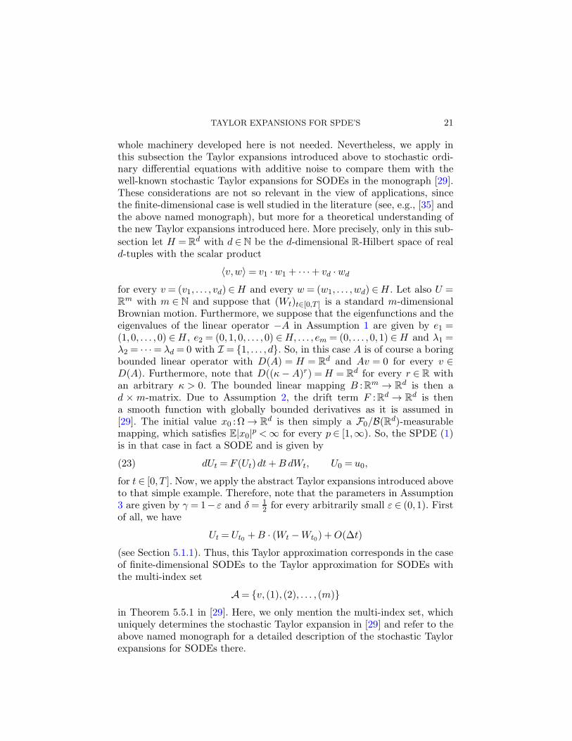
whole machinery developed here is not needed. Nevertheless, we apply inthis subsection the Taylor expansions introduced above to stochastic ordi-nary differential equations with additive noise to compare them with thewell-known stochastic Taylor expansions for SODEs in the monograph [29].These considerations are not so relevant in the view of applications, sincethe finite-dimensional case is well studied in the literature (see, e.g., [35] andthe above named monograph), but more for a theoretical understanding ofthe new Taylor expansions introduced here. More precisely, only in this sub-

section let H =Rd with d ∈N be the d-dimensional R-Hilbert space of real

d-tuples with the scalar product

〈v,w〉= v1 ·w1 + · · ·+ vd ·wd

for every v = (v1, . . . , vd) ∈H and every w = (w1, . . . ,wd) ∈H . Let also U =Rm with m ∈ N and suppose that (Wt)t∈[0,T ] is a standard m-dimensional

Brownian motion. Furthermore, we suppose that the eigenfunctions and theeigenvalues of the linear operator −A in Assumption 1 are given by e1 =(1,0, . . . ,0) ∈H , e2 = (0,1,0, . . . ,0) ∈H, . . . , em = (0, . . . ,0,1) ∈H and λ1 =λ2 = · · ·= λd = 0 with I = 1, . . . , d. So, in this case A is of course a boringbounded linear operator with D(A) = H = R

d and Av = 0 for every v ∈D(A). Furthermore, note that D((κ−A)r) =H = R

d for every r ∈ R withan arbitrary κ > 0. The bounded linear mapping B :Rm → R

d is then ad × m-matrix. Due to Assumption 2, the drift term F :Rd → R

d is thena smooth function with globally bounded derivatives as it is assumed in[29]. The initial value x0 :Ω → R

d is then simply a F0/B(Rd)-measurablemapping, which satisfies E|x0|p <∞ for every p ∈ [1,∞). So, the SPDE (1)is in that case in fact a SODE and is given by

dUt = F (Ut)dt+BdWt, U0 = u0,(23)

for t ∈ [0, T ]. Now, we apply the abstract Taylor expansions introduced aboveto that simple example. Therefore, note that the parameters in Assumption3 are given by γ = 1− ε and δ = 1

2 for every arbitrarily small ε ∈ (0,1). Firstof all, we have

Ut = Ut0 +B · (Wt −Wt0) +O(∆t)

(see Section 5.1.1). Thus, this Taylor approximation corresponds in the caseof finite-dimensional SODEs to the Taylor approximation for SODEs withthe multi-index set

A= v, (1), (2), . . . , (m)in Theorem 5.5.1 in [29]. Here, we only mention the multi-index set, whichuniquely determines the stochastic Taylor expansion in [29] and refer to theabove named monograph for a detailed description of the stochastic Taylorexpansions for SODEs there.


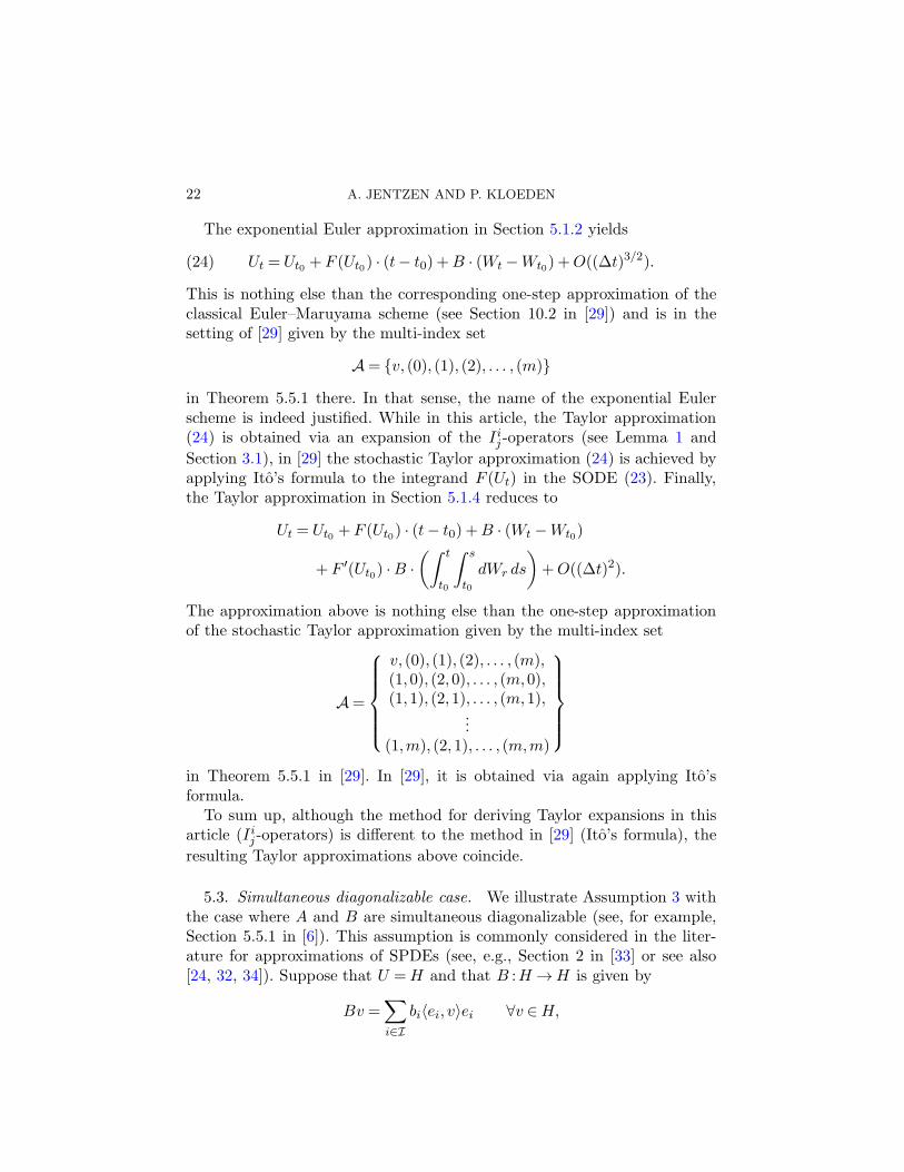
The exponential Euler approximation in Section 5.1.2 yields

Ut = Ut0 +F (Ut0) · (t− t0) +B · (Wt −Wt0) +O((∆t)3/2).(24)

This is nothing else than the corresponding one-step approximation of theclassical Euler–Maruyama scheme (see Section 10.2 in [29]) and is in thesetting of [29] given by the multi-index set

A= v, (0), (1), (2), . . . , (m)

in Theorem 5.5.1 there. In that sense, the name of the exponential Eulerscheme is indeed justified. While in this article, the Taylor approximation(24) is obtained via an expansion of the Iij -operators (see Lemma 1 and

Section 3.1), in [29] the stochastic Taylor approximation (24) is achieved byapplying Ito’s formula to the integrand F (Ut) in the SODE (23). Finally,the Taylor approximation in Section 5.1.4 reduces to

Ut = Ut0 +F (Ut0) · (t− t0) +B · (Wt −Wt0)

+F ′(Ut0) ·B ·(∫ t

t0

∫ s

t0

dWr ds

)

+O((∆t)2).

The approximation above is nothing else than the one-step approximationof the stochastic Taylor approximation given by the multi-index set

A=

v, (0), (1), (2), . . . , (m),(1,0), (2,0), . . . , (m,0),(1,1), (2,1), . . . , (m,1),

...(1,m), (2,1), . . . , (m,m)

in Theorem 5.5.1 in [29]. In [29], it is obtained via again applying Ito’sformula.

To sum up, although the method for deriving Taylor expansions in thisarticle (Iij -operators) is different to the method in [29] (Ito’s formula), the

resulting Taylor approximations above coincide.

5.3. Simultaneous diagonalizable case. We illustrate Assumption 3 withthe case where A and B are simultaneous diagonalizable (see, for example,Section 5.5.1 in [6]). This assumption is commonly considered in the liter-ature for approximations of SPDEs (see, e.g., Section 2 in [33] or see also[24, 32, 34]). Suppose that U =H and that B :H →H is given by

Bv =∑

i∈I

bi〈ei, v〉ei ∀v ∈H,


where bi, i ∈ I , is a bounded family of real numbers and ei, i ∈ I , is thefamily of eigenfunctions of the operator A (see Assumption 1). ConcerningAssumption 3, note that

∫ T

0|(κ−A)γeAsB|2HS ds

=∑

i∈I

(κ+ λi)2γb2i

(∫ T

0e−2λis ds

)

≤∑

i∈I

(κ+ λi)2γb2i

(∫ T

0e−2λise−2κs ds

)

e2κT

=∑

i∈I

(κ+ λi)2γb2i

(∫ T

0e−2(κ+λi)s ds

)

e2κT

=e2κT

2

(

∑

i∈I

b2i (κ+ λi)(2γ−1)(1− e−2(λi+κ)T )

)

≤ e2κT

2

(

∑

i∈I

b2i (κ+ λi)(2γ−1)

)

for a given γ > 0, so∫ T

0|(κ−A)γeAsB|2HS <∞

follows from∑

i∈I

b2i (κ+ λi)(2γ−1) <∞(25)

for a given γ > 0. In this case, we also have∫ t

0|eAsB|2HS ds≤Ct2δ(26)

for every t ∈ [0,1] with δ := min(γ, 12) and a constant C > 0.

5.4. Space–time white noise. This example will be a special case of theprevious one. Let H = L2((0,1),R) be the space of equivalence classes ofsquare integrable measurable functions from the interval (0,1) to R withthe scalar product and the norm

〈u, v〉=∫ 1

0u(x)v(x)dx, |u|=

√

∫ 1

0|u(x)|2 dx, u, v ∈H.


Let U = H and let B = I :H → H be the identity operator. In addition,assume that α : (0,1) → R is a bounded measurable function and that theoperator F :H →H is given by

F (v)(x) := (Fv)(x) := α(x) · v(x), x ∈ (0,1),

for all v ∈H , which clearly satisfies Assumption 2. Also note that

F ′(v)w = F (w) and F (i)(v)(w1, . . . ,wi) = 0

for all v,w,w1, . . . ,wi ∈H and all i ∈ 2,3, . . .. Furthermore, let A= ∂2

∂x2 :

D(A)⊂H →H be the Laplace operator with Dirichlet boundary condition,that is,

Au=

∞∑

n=1

−λn〈en, u〉en, u ∈H,

where

λn = π2n2, en(x) =√2 sin(nπx), x∈ (0,1),

for each n ∈ I :=N. Of course, the en, n ∈N, form an orthonormal basis ofH (Assumption 1). Additionally, we choose κ= 0.

Let t0 = 0 and T = 1. In view of (25), Assumption 3 requires γ = 14 − ε for

every arbitrarily small ε > 0. However, instead of (26), we obtain here thestronger result δ = 1

4 , since

|eAs|HS ≤C

(

1

s

)1/4

for every s ∈ (0,1] and a constant C > 0 (see Remark 2 in [32]). Finally,let u0 ∈ H be an arbitrary (deterministic) function in H , which satisfiesAssumption 4. The SPDE (1) is then given by

dUt(x) =

[

∂2

∂x2Ut(x) +α(x)Ut(x)

]

dt+ dWt, Ut(0) =Ut(1) = 0,

with U0(x) = u0(x) for x ∈ (0,1) and t ∈ [0,1]. After considering Assump-tions 1–4 for this example, we now present the Taylor approximations in thiscase. Here, ε ∈ (0, 14) is always an arbitrarily small real number in (0, 14).

5.4.1. Taylor expansion of order 1. For an approximation of Ut of orderone for small t > 0, we obtain

Ut = eAtu0 +

∫ t

0eA(t−s) dWs +O(∆t)

(see Section 5.1.1).


5.4.2. Taylor expansion of order 54 − ε. Here, we have

Ut = eAtu0 +A−1(eAt − I)Fu0 +

∫ t

0eA(t−s) dWs +O((∆t)(5/4−ε))

for an approximation of order 54 − ε (see Section 5.1.2).

5.4.3. Taylor expansion of order 54 . In the next step, we obtain


∫ t

0eA(t−s) dWs

+

(∫ t

0eA(t−s)F (eAs − I)ds

)

u0 +O((∆t)5/4)

for an approximation of order 54 (see Section 5.1.3).

5.4.4. Taylor expansion of order 32 − ε. Here, we have


∫ t

0eA(t−s)F

(∫ s

0eA(s−r) dWr

)

ds

+

(∫ t


)

u0 +

∫ t

0eA(t−s) dWs +O((∆t)(3/2−ε))

for an approximation of order 32 − ε (see Section 5.1.4).

5.4.5. Taylor expansion of order 74−ε. Since F is linear here with F ′(v)≡

F and F ′′(v)≡ 0 for all v ∈H , the approximation above is even more of order74 − ε, that is,


∫ t

0eA(t−s)F

(∫ s

0eA(s−r) dWr

)

ds

+

(∫ t


)

u0 +

∫ t

0eA(t−s) dWs +O((∆t)(7/4−ε))

(see Section 5.1.6).

5.4.6. Taylor of order 2−ε. We also consider the Taylor expansion givenby the stochastic wood

E(24,1)E(22,1)E(21,1)E(19,1)E(18,1)E(16,1)E(15,1)E(13,1)w5,

where w5 is presented in Figure 7. Since F is linear here, we see that thecorresponding Taylor approximation is the same as in the both examples


above, so we obtain


∫ t

0eA(t−s)F

(∫ s

0eA(s−r) dWr

)

ds

+

(∫ t


)

u0 +

∫ t

0eA(t−s) dWs +O((∆t)(2−ε)).

By further expansions, one can show that this approximation is in fact oforder 2.

5.5. Trace class noise. In this subsection, we compute the smoothnessparameters γ and δ in Assumption 3 for the case of trace class noise (see, e.g.,Sections 4.1 and 5.4.1 in [6]). This assumption is also commonly considered inthe literature for approximations of SPDEs (see, e.g., [15, 33]). Precisely, wesuppose that B :U →H is a Hilbert–Schmidt operator, that is, |B|HS <∞.Hence, we obtain

∫ t

0|eAsB|2HS ds≤

∫ t

0(|eAs|2 · |B|2HS)ds≤ e2κ|B|2HSt

and therefore√

∫ t

0|eAsB|2HS ds≤ eκ|B|HS

√t

for all t ∈ [0,1]. Moreover, we have∫ T

0|(κ−A)reAsB|2HS ds≤

∫ T

0|(κ−A)reAs|2|B|2HS ds

=

(∫ T

0|(κ−A)re(A−κ)seκs|2 ds

)

|B|2HS

≤(∫ T

0|(κ−A)re(A−κ)s|2 ds

)

e2κT |B|2HS

≤(∫ T

0s−2r ds

)

e2κT |B|2HS <∞

for all r ∈ [0, 12). Hence, we obtain γ = 12 − ε and δ = 1

2 for every arbitrarily

small ε ∈ (0, 12) in this situation. Now, we present the Taylor expansionsfrom Section 5.1 again in this special situation.

5.5.1. Taylor expansion of order 1. Here, we have

Ut = eA∆tUt0 +

∫ t

t0

eA(t−s)B dWs +O(∆t)

for a Taylor approximation of order 1 (see Section 5.1.1).


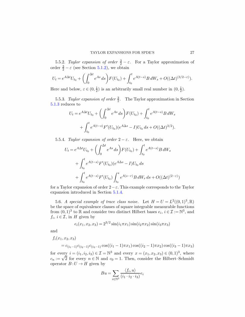
5.5.2. Taylor expansion of order 32 − ε. For a Taylor approximation of

order 32 − ε (see Section 5.1.2), we obtain

Ut = eA∆tUt0 +

(∫ ∆t

0eAs ds

)

F (Ut0) +

∫ t

t0

eA(t−s)B dWs +O((∆t)(3/2−ε)).

Here and below, ε ∈ (0, 12) is an arbitrarily small real number in (0, 12).

5.5.3. Taylor expansion of order 32 . The Taylor approximation in Section

5.1.3 reduces to

Ut = eA∆tUt0 +

(∫ ∆t

0eAs ds

)

F (Ut0) +

∫ t

t0

eA(t−s)BdWs

+

∫ t

t0

eA(t−s)F ′(Ut0)(eA∆s − I)Ut0 ds+O((∆t)3/2).

5.5.4. Taylor expansion of order 2− ε. Here, we obtain

Ut = eA∆tUt0 +

(∫ ∆t

0eAs ds

)

F (Ut0) +

∫ t

t0

eA(t−s)BdWs

+

∫ t

t0


+

∫ t

t0

eA(t−s)F ′(Ut0)

∫ s

t0

eA(s−r)BdWr ds+O((∆t)(2−ε))

for a Taylor expansion of order 2−ε. This example corresponds to the Taylorexpansion introduced in Section 5.1.4.

5.6. A special example of trace class noise. Let H = U = L2((0,1)3,R)be the space of equivalence classes of square integrable measurable functionsfrom (0,1)3 to R and consider two distinct Hilbert bases ei, i ∈ I :=N

3, andfi, i ∈ I , in H given by

ei(x1, x2, x3) = 23/2 sin(i1πx1) sin(i2πx2) sin(i3πx3)

and

fi(x1, x2, x3)

= c(i1−1)c(i2−1)c(i3−1) cos((i1 − 1)πx1) cos((i2 − 1)πx2) cos((i3 − 1)πx3)

for every i = (i1, i2, i3) ∈ I = N3 and every x = (x1, x2, x3) ∈ (0,1)3, where

cn :=√2 for every n ∈ N and c0 = 1. Then, consider the Hilbert–Schmidt

operator B :U →H given by

Bu=∑

i∈N3

〈fi, u〉(i1 · i2 · i3)

ei


for all u ∈ U = H . Moreover, let λi, i ∈ N3, be a family of real numbers

given by λi = π2(i21 + i22 + i23) for all i = (i1, i2, i3) ∈ N3. Finally, consider

A= ( ∂2

∂x21+ ∂2

∂x22+ ∂2

∂x23) :D(A)⊂H →H (with Dirichlet boundary conditions)

given by

Av =∑

i∈N3

−λi〈ei, v〉ei

for all v ∈D(A), where D(A) is given by

D(A) =

v ∈H

∣

∣

∣

∣

∑

i∈N3

(i21 + i22 + i23)|〈ei, v〉|2

.

Then, the SPDE (1) reduces to

dUt(x) =

[(

∂2

∂x21+

∂2

∂x22+

∂2

∂x23

)

Ut(x) +F (Ut(x))

]

dt+√

QdWt(x)

with U |∂(0,1)3 = 0 for x ∈ (0,1)3 and t ∈ [0, T ]. Assumptions 1–4 are fulfilled

with δ = 12 and γ = 1

2 − ε for every arbitrarily small ε ∈ (0, 12 ) (see Section5.5). The Taylor approximations in that situation are presented in Section5.5.

6. Numerical schemes based on the Taylor expansions. In this section,some numerical schemes based on the Taylor expansions in this article arepresented. We refer to [21, 22, 24, 25] for estimations of the convergenceorders of these schemes and also for numerical simulations for these schemes.

For numerical approximations of SPDEs, one has to discretize both thetime interval [0, T ] and the R-Hilbert space H . For the discretization of thespace H , we use a spectral Galerkin approximation based on the eigenfunc-tions of the linear operator A :D(A)⊂H →H . More precisely, let (IN )N∈N

be a sequence of increasing finite nonempty subsets of I , that is, ∅ 6= IN ⊂IM ⊂ I for all N,M ∈ N with N ≤ M and let HN := span〈ei, i ∈ IN 〉 bethe finite-dimensional span of |IN |-eigenfunctions for N ∈N. The boundedlinear mappings PN :H →HN are then given by PN (v) =

∑

i∈IN〈ei, v〉ei for

every v ∈H and every N ∈N.

6.1. The exponential Euler scheme. Based on the Taylor approxima-tion in Sections 3.2 and 5.1.2, we consider the family of random variablesY N,Mk :Ω→HN , k = 0,1, . . . ,M , N,M ∈N, given by Y N,M

0 = PN (u0) and

Y N,Mk+1 = eAT/MY N,M

k +

(∫ T/M

0eAs ds

)

(PNF )(Y N,Mk )

(27)

+ PN

(∫ (k+1)T/M

kT/MeA((k+1)T/M−s)BdWs

)


for every k = 0,1, . . . ,M − 1 and every N,M ∈N. This scheme is introducedand analyzed in [24]. As already mentioned, it is called the exponential Eulerscheme there.

In the setting of deterministic PDEs, that is, in the case B = 0, thisscheme reduces to


k +

(∫ T/M

0eAs ds

)

(PNF )(Y N,Mk )

for every k = 0,1, . . . ,M − 1 and every N,M ∈ N. This scheme and similarschemes, usually referred as exponential integrators, have for deterministicPDEs been intensively studied in the literature (see, e.g., [3–5, 16–19, 27,30, 31, 36]). Such schemes are easier to simulate than may seem on the firstsight (see [4]). In the stochastic setting, we refer to Sections 3 and 4 in [24]for a detailed description for the simulation of the scheme (27), in particular,for the generation of the random variables used there.

6.2. The Taylor scheme indicated by Section 5.1.3. In view of Section5.1.3, we obtain the Taylor scheme Y N,M

k :Ω→HN , k = 0,1, . . . ,M , N,M ∈N, given by Y N,M

0 = PN (u0) and


k +

(∫ T/M

0eAs ds

)

(PNF )(Y N,Mk )

+

∫ (k+1)T/M

kT/MeA((k+1)T/M−s)(PNF ′)(Y N,M

k )

× ((eA(s−kT/M) − I)Y N,Mk )ds

+ PN

(∫ (k+1)T/M

kT/MeA((k+1)T/M−s)BdWs

)

for every k = 0,1, . . . ,M − 1 and every N,M ∈N.

6.3. The Taylor scheme indicated by Section 5.1.4. The Taylor approx-imation in Section 5.1.4 yields the Taylor scheme Y N,M

k :Ω → HN , k =

0,1, . . . ,M , N,M ∈N, given by Y N,M0 = PN (u0) and


k +

(∫ T/M

0eAs ds

)

(PNF )(Y N,Mk )

+

∫ (k+1)T/M

kT/MeA((k+1)T /M−s)(PNF ′)(Y N,M

k )

× ((eA(s−kT/M) − I)Y N,Mk )ds


+

∫ (k+1)T/M

kT/MeA((k+1)T /M−s)(PNF ′)(Y N,M

k )

×(

PN

(∫ s

kT/MeA(s−u)BdWu

))

ds

+PN

(∫ (k+1)T/M

kT/MeA((k+1)T/M−s)B dWs

)

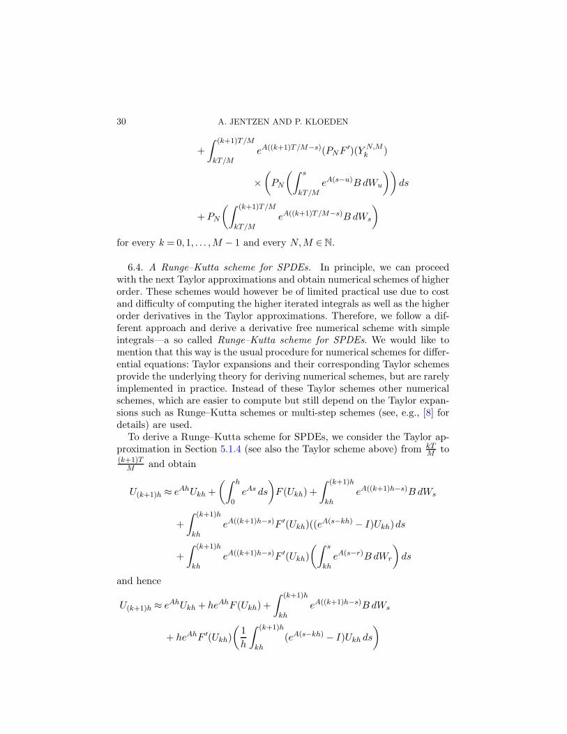
for every k = 0,1, . . . ,M − 1 and every N,M ∈N.

6.4. A Runge–Kutta scheme for SPDEs. In principle, we can proceedwith the next Taylor approximations and obtain numerical schemes of higherorder. These schemes would however be of limited practical use due to costand difficulty of computing the higher iterated integrals as well as the higherorder derivatives in the Taylor approximations. Therefore, we follow a dif-ferent approach and derive a derivative free numerical scheme with simpleintegrals—a so called Runge–Kutta scheme for SPDEs. We would like tomention that this way is the usual procedure for numerical schemes for differ-ential equations: Taylor expansions and their corresponding Taylor schemesprovide the underlying theory for deriving numerical schemes, but are rarelyimplemented in practice. Instead of these Taylor schemes other numericalschemes, which are easier to compute but still depend on the Taylor expan-sions such as Runge–Kutta schemes or multi-step schemes (see, e.g., [8] fordetails) are used.

To derive a Runge–Kutta scheme for SPDEs, we consider the Taylor ap-proximation in Section 5.1.4 (see also the Taylor scheme above) from kT

M to(k+1)T

M and obtain

U(k+1)h ≈ eAhUkh +

(∫ h

0eAs ds

)

F (Ukh) +

∫ (k+1)h

kheA((k+1)h−s)BdWs

+

∫ (k+1)h

kheA((k+1)h−s)F ′(Ukh)((e

A(s−kh) − I)Ukh)ds

+

∫ (k+1)h

kheA((k+1)h−s)F ′(Ukh)

(∫ s

kheA(s−r)BdWr

)

ds

and hence

U(k+1)h ≈ eAhUkh + heAhF (Ukh) +

∫ (k+1)h


+ heAhF ′(Ukh)

(

1

h

∫ (k+1)h

kh(eA(s−kh) − I)Ukh ds

)


+ heAhF ′(Ukh)

(

1

h

∫ (k+1)h

kh

∫ s

kheA(s−r)BdWr ds

)

≈ eAhUkh + heAhF (Ukh) +

∫ (k+1)h


+ heAhF ′(Ukh)

[

1

h

∫ (k+1)h

kh(eA(s−kh) − I)

∫ kh

0eA(kh−r)BdWr ds

]

+ heAhF ′(Ukh)

(

1

h

∫ (k+1)h

kh

∫ s

kheA(s−r)BdWr ds

)

with h := TM for k = 0,1, . . . ,M − 1 and M ∈N. This yields

U(k+1)h ≈ eAhUkh + heAhF (Ukh +ZMk ) +

∫ (k+1)h


with the random variables

ZMk =

1

h

∫ (k+1)h

kh(eA(s−kh) − I)

∫ kh

0eA(kh−r)BdWr ds

+1

h

∫ (k+1)h

kh

∫ s

kheA(s−r)B dWr ds

for k = 0,1, . . . ,M − 1 and M ∈ N. The corresponding numerical schemeY N,Mk :Ω→HN , k = 0,1, . . . ,M , N,M ∈N, is then given by Y N,M

0 = PN (u0)and


k +T

MeAT/M (PNF )(Y N,M

k +PN (ZMk ))

+PN

(∫ (k+1)T/M

kT/MeA((k+1)T/M−s)B dWs

)

for every k = 0,1, . . . ,M −1 and every N,M ∈N. This Runge–Kutta schemefor SPDEs is introduced and analyzed in [21]. Under non-global Lipschitzcoefficients of the SPDE, it is analyzed in [22]. Note that the random vari-ables occurring in the scheme above are Gaussian distributed and thereforeeasy to simulate (see also Remark 1 and [21, 22] for details). More pre-cisely, in the case of one-dimensional stochastic reaction diffusion equationswith space–time white noise it is shown in the articles cited above that thisscheme converges with the overall order 1

4—with respect to the number ofindependent standard normal distributed random variables and the numberof arithmetical operations used to compute the scheme instead of the overallorder 1

6 of classical numerical schemes (see, for instance, [7, 12, 13, 42]) suchas the linear implicit Euler scheme.


7. Proofs.

7.1. Proofs of (6) and (7).

Lemma 1. Let Assumptions 1–4 be fulfilled and let i ∈N be given. Then,we have

I01∗ = I01 + I11∗ [I00 ] + I11∗ [I

01∗ ] + I11∗ [I

02 ]

and

Ii1∗ [g1, . . . , gi] = Ii1[g1, . . . , gi] + I(i+1)1∗ [I00 , g1, . . . , gi]

+ I(i+1)1∗ [I01∗ , g1, . . . , gi] + I

(i+1)1∗ [I02 , g1, . . . , gi]

for all g1, . . . , gi ∈ P.

Proof. We begin with the first equation. Since we have

F (Us) = F (Ut0) +

∫ 1

0F ′(Ut0 + r(Us −Ut0))(Us −Ut0)dr

= F (Ut0) +

∫ 1

0F ′(Ut0 + r∆Us)(∆Us)dr

= F (Ut0) +

∫ 1

0F ′(Ut0 + r∆Us)(I

00 (s))dr

+

∫ 1

0F ′(Ut0 + r∆Us)(I

01∗(s))dr+

∫ 1

0F ′(Ut0 + r∆Us)(I

02 (s))dr

for every s ∈ [t0, T ] due to the fundamental theorem of calculus and (5), weobtain

I01∗(t) =

∫ t

t0

eA(t−s)F (Us)ds

=

∫ t

t0

eA(t−s)F (Ut0)ds+

∫ t

t0

eA(t−s)

(∫ 1

0F ′(Ut0 + r∆Us)(I

00 (s))dr

)

ds

+

∫ t

t0

eA(t−s)

(∫ 1

0F ′(Ut0 + r∆Us)(I

01∗(s))dr

)

ds

+

∫ t

t0

eA(t−s)

(∫ 1

0F ′(Ut0 + r∆Us)(I

02 (s))dr

)

ds,

which implies

I01∗(t) = I01 (t) + I11∗ [I00 ](t) + I11∗ [I

01∗ ](t) + I11∗ [I

02 ](t)


for all t ∈ [t0, T ]. Moreover, we have

∫ 1

0F (i)(Ut0 + r∆Us)(g1(s), . . . , gi(s))

(1− r)(i−1)

(i− 1)!dr

=

[

−F (i)(Ut0 + r∆Us)(g1(s), . . . , gi(s))(1− r)i

i!

]r=1

r=0

+

∫ 1

0F (i+1)(Ut0 + r∆Us)(∆Us, g1(s), . . . , gi(s))

(1− r)i

i!dr

=1

i!F (i)(Ut0)(g1(s), . . . , gi(s))

+

∫ 1

0F (i+1)(Ut0 + r∆Us)(∆Us, g1(s), . . . , gi(s))

(1− r)i

i!dr

for all s ∈ [t0, T ] and all g1, . . . , gi ∈P due to integration by parts and there-fore, we also obtain the second equation.

7.2. Proof of Theorem 1. For the proof of Theorem 1, we need the fol-lowing lemma.

Lemma 2. Let X : [t0, T ]×Ω→ [0,∞) be a predictable stochastic process.Then, we obtain

∣

∣

∣

∣

∫ t

t0

Xs ds

∣

∣

∣

∣

Lr

≤∫ t

t0

|Xs|Lr ds

for every t ∈ [t0, T ] and every r ∈ [1,∞), where both sides could be infinite.

Proof. First, we consider the case, where Xt ≤ C is bounded by aconstant C > 0 for all t ∈ [0, T ]. Here, we have

E

[(∫ t

t0

Xs ds

)r]

=

∫ t

t0

E

[(∫ t

t0

Xu du

)(r−1)

Xs

]

ds

≤∫ t

t0

|Xs|Lr ds

(

E

[(∫ t

t0

Xu du

)r])((r−1)/r)

for every t ∈ [t0, T ] and every r ∈ [1,∞) due to Holder’s inequality. Since

E

[(∫ t

t0

Xu du

)r]

<∞

is finite for every t ∈ [t0, T ] and every r ∈ [1,∞) due to the boundednessof X : [t0, T ]×Ω→ [0,∞), we obtain the assertion. In the general case, we


can approximation the stochastic process (Xt)t∈[0,T ] by bounded processes

(XNt )t∈[0,T ] for N ∈N given by

XNt := min(N,Xt)

for all t ∈ [0, T ] and all N ∈N. This shows the assertion.

We also need the Burkholder–Davis–Gundy inequality in infinite dimen-sions (see Lemma 7.7 in [6]).

Lemma 3. Let X : [t0, T ]×Ω→HS(U,H) be a predictable stochastic pro-

cess with E∫ Tt0|Xs|2HS <∞. Then, we obtain

∣

∣

∣

∣

∫ t

t0

Xs dWs

∣

∣

∣

∣

Lp

≤ p

(∫ t

t0

||Xs|HS|2Lp ds

)1/2

for every t ∈ [t0, T ] and every p ∈ [1,∞), where both sides could be infinite.

In view of the definitions of the mappings Φ and Ψ, Theorem 1 immedi-ately follows from the next lemma. For this, the subset ST′ ⊂ ST of stochas-tic trees given by

ST′ :=

t= (t′, t′′) ∈ ST|∀k ∈ nd(t) : ((∃l ∈ nd(t) : t′(l) = k)

=⇒ (t′′(k) ∈ 1,1∗))

is used.

Lemma 4. Let t= (t′, t′′) ∈ ST′ be an arbitrary stochastic tree in ST

′.Then, for each p≥ 1, there exists a constant Cp > 0 such that

(E[|Φ(t)(t)|p])1/p ≤Cp · (t− t0)ord(t)

holds for all t ∈ [t0, T ], where Cp is independent of t and t0 but depends onp, t, T and the SPDE (1).

Proof. Due to Jensen’s inequality, we can assume without loss of gen-erality that p ∈ [2,∞) holds. We will prove now the assertion by inductionwith respect to the number of nodes l(t) ∈N.

In the base case l(t) = 1, we have Φ(t) = I0t′′(1) by definition. Hence, we

obtain

|Φ(t)(t)|Lp = |I0t′′(1)(t)|Lp = |I00 (t)|Lp = |(eA∆t − I)Ut0 |Lp

≤ |(κ−A)−γ(eA∆t − I)| · |(κ−A)γUt0 |Lp


= |(κ−A)−γ(e(A−κ)∆t − e−κ∆t)| · eκ∆t · |(κ−A)γUt0 |Lp

≤ |(κ−A)−γ(e(A−κ)∆t − e−κ∆t)| · eκT ·(

sup0≤s≤T

|(κ−A)γUs|Lp

)

≤ Cp · |(κ−A)−γ(e(A−κ)∆t − e−κ∆t)|and therefore

|Φ(t)(t)|Lp ≤Cp · (|(κ−A)−γ(e(A−κ)∆t − I)|+ |(κ−A)−γ(I − e−κ∆t)|)

≤Cp · (|(κ−A)−γ(e(A−κ)∆t − I)|+ |(I − e−κ∆t)|)≤Cp · (∆t)γ +Cp · (∆t)≤Cp · (∆t)γ

for every t ∈ [t0, T ] in the case t′′(1) = 0. Here and below, Cp > 0 is a con-

stant, which changes from line to line but is independent of t and t0. More-over, by Lemma 2, we obtain

|Φ(t)(t)|Lp = |I0t′′(1)(t)|Lp = |I01∗(t)|Lp =

∣

∣

∣

∣

∫ t

t0

eA(t−s)F (Us)ds

∣

∣

∣

∣

Lp

≤∫ t

t0

(|eA(t−s)F (Us)|Lp)ds≤Cp ·(∫ t

t0

|F (Us)|Lp ds

)

≤Cp ·(∫ t

t0

(1 + |Us|Lp)ds

)

≤Cp · (∆t)

for every t ∈ [t0, T ] in the case t′′(1) = 1∗ and

|Φ(t)(t)|Lp = |I0t′′(1)(t)|Lp = |I01 (t)|Lp

=

∣

∣

∣

∣

∫ t

t0

eA(t−s)F (Ut0)ds

∣

∣

∣

∣

Lp

≤∫ t

t0

(|eA(t−s)F (Ut0)|Lp)ds≤Cp ·(∫ t

t0

|F (Ut0)|Lp ds

)

≤ Cp ·(∫ t

t0

(1 + |Ut0 |Lp)ds

)

≤Cp · (∆t)

for every t ∈ [t0, T ] in the case t′′(1) = 1. Finally, due to Lemma 3, we obtain

|Φ(t)(t)|Lp = |I0t′′(1)(t)|Lp = |I02 (t)|Lp =

∣

∣

∣

∣

∫ t

t0

eA(t−s)BdWs

∣

∣

∣

∣

Lp

≤ Cp ·(∫ t

t0

||eA(t−s)B|HS|2Lp ds

)1/2

≤ Cp ·(∫ (∆t)

0|eAsB|2HS ds

)1/2


≤ Cp · (∆t)δ

for every t ∈ [t0, T ] in the case t′′(1) = 2. This shows |Φ(t)(t)|Lp ≤ Cp ·

(∆t)ord(t) for every t ∈ [t0, T ] in the base case l(t) = 1.Suppose now that l(t) ∈ 2,3, . . .. Since t= (t′, t′′) ∈ ST

′, we must havet′′(1) ∈ 1,1∗. Let t1, . . . , tn ∈ ST

′ with n ∈ N be the subtrees of t. Notethat t1, . . . , tn are indeed in ST

′. Then, by definition, we have

Φ(t)(t) = Int′′(1)[Φ(t1), . . . ,Φ(tn)](t)

for every t ∈ [t0, T ]. Therefore, by Lemma 2, we obtain

|Φ(t)(t)|Lp = |Int′′(1)[Φ(t1), . . . ,Φ(tn)](t)|= |In1∗ [Φ(t1), . . . ,Φ(tn)](t)|Lp

=

∣

∣

∣

∣

∫ t

t0

eA(t−s)

(∫ 1

0F (n)(Ut0 + r∆Us)

× (Φ(t1)(s), . . . ,Φ(tn)(s))(1− r)n−1

(n− 1)!dr

)

ds

∣

∣

∣

∣

Lp

≤ Cp ·∫ t

t0

∣

∣

∣

∣

∫ 1

0F (n)(Ut0 + r∆Us)

× (Φ(t1)(s), . . . ,Φ(tn)(s))(1− r)n−1

(n− 1)!dr

∣

∣

∣

∣

Lp

ds

≤ Cp ·∫ t

t0

∫ 1

0

∣

∣

∣

∣

F (n)(Ut0 + r∆Us)

× (Φ(t1)(s), . . . ,Φ(tn)(s))(1− r)n−1

(n− 1)!

∣

∣

∣

∣

Lp

dr ds

≤ Cp ·∫ t

t0

∫ 1

0|F (n)(Ut0 + r∆Us)(Φ(t1)(s), . . . ,Φ(tn)(s))|Lp dr ds

≤ Cp ·∫ t

t0

∫ 1

0||Φ(t1)(s)| · · · |Φ(tn)(s)||Lp dr ds

and hence

|Φ(t)(t)|Lp ≤ Cp ·∫ t

t0

||Φ(t1)(s)| · · · |Φ(tn)(s)||Lp ds

≤ Cp ·(∫ t

t0

|Φ(t1)(s)|Lpn · · · |Φ(tn)(s)|Lpn ds

)

≤ Cp ·(∫ t

t0

((∆s)ord(t1) · · · (∆s)ord(tn))ds

)

≤ Cp · (∆t)(1+ord(t1)+···+ord(tn)) =Cp · (∆t)ord(t)


for every t ∈ [t0, T ] in the case t′′(1) = 1∗, since l(t1), . . . , l(tn)≤ l(t)− 1 and

we can apply the induction hypothesis to the subtrees. A similar calculationshows the result when t

′′(1) = 1.

7.3. Properties of the stochastic convolution.

Lemma 5. Let Assumptions 1 and 3 be fulfilled. Then, there exists anadapted stochastic process O :Ω→C([0, T ],H) with continuous sample paths,

which is a modification of the stochastic convolution∫ t0 e

A(t−s)B dWs, t ∈[0, T ], that is, we have

P

[∫ t

0eA(t−s)BdWs =Ot

]

= 1

for all t ∈ [0, T ].

Proof. Let Z : [0, T ]×Ω→H be an arbitrary adapted stochastic pro-cess with

Zt =

∫ t

0eA(t−s)BdWs, P-a.s.,

for all t ∈ [0, T ]. Due to Assumption 3, such an adapted stochastic processexists. Moreover, Z : [0, T ]×Ω→H is centered and square integrable with

E|Zt|2 =∫ t

0|eA(t−s)B|2HS ds=

∫ t

0|eAsB|2HS ds

for all t ∈ [0, T ]. Let θ := min(δ, γ), p≥ 2 and 0≤ t1 ≤ t2 ≤ T be given. Then,we have

Zt2 −Zt1 =

∫ t2

t1

eA(t2−s)BdWs

+

∫ t1

0(eA(t2−s) − eA(t1−s))BdWs, P-a.s.,

and

|Zt2 −Zt1 |Lp ≤ p

(∫ t2

t1

||eA(t2−s)B|HS|2Lp ds

)1/2

+ p

(∫ t1

0||(eA(t2−s) − eA(t1−s))B|HS|

2Lp ds

)1/2

= p

(∫ (t2−t1)

0|eAsB|2HS ds

)1/2

+ p

(∫ t1

0|(eA(t2−t1) − I)eAsB|2HS ds

)1/2


due to Lemma 3. Hence, due to Assumption 3, we obtain

|Zt2 −Zt1 |Lp ≤ C(t2 − t1)δ

+C|(κ−A)−γ(eA(t2−t1) − I)|(∫ t1


)1/2

≤ C(t2 − t1)δ +C(t2 − t1)

γ

(∫ T


)1/2

≤ C(t2 − t1)δ +C(t2 − t1)

γ ≤C(t2 − t1)θ,

where C > 0 is a constant changing from line to line. Since θ > 0 is greaterthan zero and since p≥ 2 was arbitrary, there exists a version of (Zt)t∈[0,T ]

with continuous sample paths due to Kolmogorov’s theorem (see, e.g., Chap-ter 3 in [6]).

Acknowledgments. We strongly thank the anonymous referee for hiscareful reading and his very valuable advice.

REFERENCES

[1] Burrage, K. and Burrage, P. M. (2000). Order conditions of stochastic Runge–Kutta methods by B-series. SIAM J. Numer. Anal. 38 1626–1646. MR1813248

[2] Butcher, J. C. (1987). The Numerical Analysis of Ordinary Differential Equations:Runge–Kutta and General Linear methods. Wiley, Chichester. MR878564

[3] Berland, H., Owren, B. and Skaflestad, B. (2005). B-series and order conditionsfor exponential integrators. SIAM J. Numer. Anal. 43 1715–1727. MR2182146

[4] Berland, H., Skaflestad, B. and Wright, W. (2007). Expint—AMatlab packagefor exponential integrators. ACM Trans. Math. Software 33 1–17.

[5] Cox, S. M. and Matthews, P. C. (2002). Exponential time differencing for stiffsystems. J. Comput. Phys. 176 430–455. MR1894772

[6] Da Prato, G. and Zabczyk, J. (1992). Stochastic Equations in Infinite Dimensions.Encyclopedia of Mathematics and Its Applications 44. Cambridge Univ. Press,Cambridge. MR1207136

[7] Davie, A. M. and Gaines, J. G. (2001). Convergence of numerical schemes for thesolution of parabolic stochastic partial differential equations. Math. Comp. 70121–134. MR1803132

[8] Deuflhard, P. and Bornemann, F. (2002). Scientific Computing with OrdinaryDifferential Equations. Texts in Applied Mathematics 42. Springer, New York.MR1912409

[9] Engel, K. and Nagel, R. (1999). One-Parameter Semigroups for Linear EvolutionEquations. Springer, Berlin.

[10] Gradinaru, M., Nourdin, I. and Tindel, S. (2005). Ito’s- and Tanaka’s-type for-mulae for the stochastic heat equation: The linear case. J. Funct. Anal. 228

114–143. MR2170986[11] Gyongy, I. (1998). A note on Euler’s approximations. Potential Anal. 8 205–216.

MR1625576

http://www.ams.org/mathscinet-getitem?mr=1813248










[12] Gyongy, I. (1998). Lattice approximations for stochastic quasi-linear parabolic par-tial differential equations driven by space-time white noise. I. Potential Anal. 9

1–25. MR1644183[13] Gyongy, I. (1999). Lattice approximations for stochastic quasi-linear parabolic par-

tial differential equations driven by space-time white noise. II. Potential Anal.

11 1–37. MR1699161[14] Gyongy, I. and Krylov, N. (2003). On the splitting-up method and stochastic

partial differential equations. Ann. Probab. 31 564–591. MR1964941[15] Hausenblas, E. (2003). Approximation for semilinear stochastic evolution equations.

Potential Anal. 18 141–186. MR1953619

[16] Hochbruck, M., Lubich, C. and Selhofer, H. (1998). Exponential integratorsfor large systems of differential equations. SIAM J. Sci. Comput. 19 1552–1574.

MR1618808[17] Hochbruck, M. and Ostermann, A. (2005). Explicit exponential Runge–Kutta

methods for semilinear parabolic problems. SIAM J. Numer. Anal. 43 1069–

1090. MR2177796[18] Hochbruck, M. and Ostermann, A. (2005). Exponential Runge–Kutta methods

for parabolic problems. Appl. Numer. Math. 53 323–339. MR2128529[19] Hochbruck, M., Ostermann, A. and Schweitzer, J. (2008/09). Exponential

Rosenbrock-type methods. SIAM J. Numer. Anal. 47 786–803. MR2475962

[20] Jentzen, A. (2007). Numerische Verfahren hoher Ordnung fur zufallige Differential-gleichungen, Diplomarbeit. Johann Wolfgang Geothe Univ. Frankfurt am Main.

[21] Jentzen, A. (2009). Higher order pathwise numerical approximations of SPDEs withadditive noise. Submitted.

[22] Jentzen, A. (2009). Pathwise numerical approximations of SPDEs with additive

noise under non-global Lipschitz coefficients. Potential Anal. 4 375–404.[23] Jentzen, A. and Kloeden, P. E. (2009). Pathwise Taylor schemes for random

ordinary differential equations. BIT 49 113–140. MR2486131[24] Jentzen, A. and Kloeden, P. E. (2009). Overcoming the order barrier in the nu-

merical approximation of stochastic partial differential equations with additive

space-time noise. Proc. R. Soc. Lond. Ser. A Math. Phys. Eng. Sci. 465 649–667.MR2471778

[25] Jentzen, A. andKloeden, P. E. (2009). The numerical approximation of stochasticpartial differential equations. Milan J. Math. 77 205–244.

[26] Jentzen, A., Kloeden, P. E. and Neuenkirch, A. (2009). Pathwise approximation

of stochastic differential equations on domains: Higher order convergence rateswithout global Lipschitz coefficients. Numer. Math. 112 41–64. MR2481529

[27] Kassam, A.-K. and Trefethen, L. N. (2005). Fourth-order time-stepping for stiffPDEs. SIAM J. Sci. Comput. 26 1214–1233. MR2143482

[28] Kloeden, P. E. and Jentzen, A. (2007). Pathwise convergent higher order numeri-

cal schemes for random ordinary differential equations. Proc. R. Soc. Lond. Ser.A Math. Phys. Eng. Sci. 463 2929–2944. MR2360184

[29] Kloeden, P. E. and Platen, E. (1992). Numerical Solution of Stochastic Differ-ential Equations. Applications of Mathematics (New York) 23. Springer, Berlin.MR1214374

[30] Krogstad, S. (2005). Generalized integrating factor methods for stiff PDEs. J. Com-put. Phys. 203 72–88. MR2104391

[31] Lawson, J. D. (1967). Generalized Runge–Kutta processes for stable systems withlarge Lipschitz constants. SIAM J. Numer. Anal. 4 372–380. MR0221759


















[32] Muller-Gronbach, T. and Ritter, K. (2007). Lower bounds and nonuniform timediscretization for approximation of stochastic heat equations. Found. Comput.Math. 7 135–181. MR2324415

[33] Muller-Gronbach, T. and Ritter, K. (2007). An implicit Euler scheme with non-uniform time discretization for heat equations with multiplicative noise. BIT 47

393–418. MR2334046[34] Muller-Gronbach, T., Ritter, K. and Wagner, T. (2008). Optimal pointwise

approximation of a linear stochastic heat equation with additive space-timewhite noise. In Monte Carlo and Quasi-Monte Carlo Methods 2006 577–589.Springer, Berlin. MR2479247

[35] Milstein, G. N. (1995). Numerical Integration of Stochastic Differential Equations.Mathematics and Its Applications 313. Kluwer, Dordrecht. MR1335454

[36] Ostermann, A., Thalhammer, M. and Wright, W. M. (2006). A class of explicitexponential general linear methods. BIT 46 409–431. MR2238680

[37] Prevot, C. and Rockner, M. (2007). A Concise Course on Stochastic Partial Dif-ferential Equations. Lecture Notes in Math. 1905. Springer, Berlin. MR2329435

[38] Roßler, A. (2009). Runge–Kutta Methods for the Numerical Solution of StochasticDifferential Equations. Shaker, Aachen.

[39] Roßler, A. (2004). Stochastic Taylor expansions for the expectation of functionalsof diffusion processes. Stoch. Anal. Appl. 22 1553–1576. MR2095070

[40] Roßler, A. (2006). Rooted tree analysis for order conditions of stochastic Runge–Kutta methods for the weak approximation of stochastic differential equations.Stoch. Anal. Appl. 24 97–134. MR2198539

[41] Sell, G. R. and You, Y. (2002). Dynamics of Evolutionary Equations. AppliedMathematical Sciences 143. Springer, New York. MR1873467

[42] Shardlow, T. (1999). Numerical methods for stochastic parabolic PDEs. Numer.Funct. Anal. Optim. 20 121–145. MR1683281

Institute of Mathematics

Johann Wolfgang Goethe University

Robert-Mayer-Str. 6-10

D-60325 Frankfurt am Main

Germany

E-mail: [email protected]@math.uni-frankfurt.de











mailto:[email protected]

mailto:[email protected]

Johann Wolfgang Goethe University, Frankfurt am Main · Johann Wolfgang Goethe University,...

Documents

Transcript of Johann Wolfgang Goethe University, Frankfurt am Main · Johann Wolfgang Goethe University,...