Job Loss, Job Finding, and Unemployment in the U.S.Economy over the Past Fifty Years ∗

Robert E. HallHoover Institution and Department of Economics, Stanford University

National Bureau of Economic Researchrehall@stanford.edu

stanford.edu/˜rehall.

September 15, 2005

Abstract

New data compel a new view of events in the labor market during a recession.Unemployment rises almost entirely because jobs become harder to find. Recessionsinvolve little increase in the flow of workers out of jobs. Another important findingfrom new data is that a large fraction of workers departing jobs move to new jobs with-out intervening unemployment. I develop estimates of separation rates and job-findingrates for the past 50 years, using historical data informed by detailed recent data. Theseparation rate is nearly constant while the job-finding rate shows high volatility atbusiness-cycle and lower frequencies. I review modern theories of fluctuations in thejob-finding rate. The challenge to these theories is to identify mechanisms in the labormarket that amplify small changes in driving forces into fluctuations in the job-findingrate of the high magnitude actually observed. In the standard theory developed overthe past two decades, the wage moves to offset driving forces and the predicted magni-tude of changes in the job-finding rate is tiny. New models overcome this property byinvoking a new form of sticky wages or by introducing information and other frictionsinto the employment relationship.

∗Presented to the NBER Macro Annual Conference, April 2005. This research is part of the program onEconomic Fluctuations and Growth of the NBER. I thank the editors and discussants, Narayana Kocherlakota,Michael Krause, Thomas Lubik, Robert Shimer, and Frank Wolak for comments, suggestions, and data. Afile containing data and programs is available at Stanford.edu/˜rehall

1

1 Introduction

The turnover view of unemployment has a firm grip on modern thinking about joblessness

in the United States. Unemployment occurs when a worker departs from a job and spends

time finding a new job. In addition, unemployment arises when a person looks for a new job

after a period out of the labor force. Job-seekers find new jobs at monthly rates ranging from

10 to 40 percent. Unemployment varies positively with the separation rate and negatively

with the job-finding rate.

For many years, students of the labor market believed that recessions—periods of

sharply rising unemployment—were the result of higher separation rates from jobs as well

as lower job-finding rates. In this view, a recession begins with a wave of layoffs, mainly in

cyclical durable-goods industries. As the labor market becomes clogged with job-seekers,

job-finding rates go down and the duration of unemployment rises. The second part of this

account is not in dispute. Much of this paper will focus on the large movements at cyclical

and sub-cyclical frequencies in the job-finding rate. But new research and new data have

challenged the first part. The new view is that separations are not an important part of the

story of rising unemployment in recessions. Unemployment is high in a recession because

jobs are hard to find, not because more job-seekers have been dumped into the labor market

by elevated separation rates.

The new view puts the focus on the hiring decision as the central topic for understanding

cyclical variation in unemployment. The labor market goes through extended periods when

the number of new hires remains constant despite the availability of large numbers of job-

seekers. The surplus created by a new hire appears to be greater in those periods than when

unemployment is lower. Productivity is hardly cyclical, so the marginal product of a new

hire is as high as ever. The opportunity cost of a job-seeker is lower in a soft labor market.

The surplus arises from the gap between the marginal product and the opportunity cost. In

spite of the substantial joint gain from a hire, employers do not raise hiring rates during

periods of high unemployment. Slack labor markets persist for several years following a

2

recession. The challenge to unemployment theory is to explain why hiring remains stable.

Arbitrage does not close the gap in the labor market as fast as it seems to in other markets.

In addition to experiencing periods of high unemployment following every recession, the

economy suffers from chronically high unemployment for extended periods, such as the

1970s and 1980s. These periods are equally puzzling.

I begin by documenting the surprising proposition that layoffs and other separations

do not rise during the time when output and employment are falling at the beginning of a

recession. The evidence is strongest for the most recent recession, thanks to a survey that

measures separations directly, across the entire economy. For earlier periods, the evidence

is less direct but reasonably compelling. I stress that the proposition doesnot mean that

employers make all employment adjustments through variations in hires and keep separa-

tions at a constant level independent of the need to adjust their employment levels. The

point is that the changes in separation rates that accompany employment changes at the

industry or aggregate level are tiny compared to the regular flow of workers out of jobs.

Job-seekers are unemployed, out of the labor force, or employed in jobs they would

like to leave. I show that only a minority of new hires come from the unemployed. Hence

the measurement of a job-finding rate would ideally incorporate job-seekers in all three

statuses—unemployed, out of the labor force, or employed. Despite the importance of the

employed among job-seekers, I am unable to include them for lack of data. I am able to

include a group of those out of the labor force whose behavior is known to be similar to

those counted as unemployed. I then calculate a job-finding rate as the ratio of new hires

to my measure of job-seekers. The job-finding rate is highly cyclical—it plunges in every

recession. It also has important movements at lower frequencies—it was high in the 1960s

and 1990s and low in the 1970s and 1980s. One of my themes is that the subcyclical

movements of the job-finding rates are just as informative and puzzling as the cyclical

movements. A full understanding of the labor market requires a unified explanation of the

cyclical and sub-cyclical movements.

3

The past few years have seen an explosion of new models of the job-finding process.

The models share some common features. In particular, information limitations constrain

the labor market. Job-seekers and employers are imperfectly informed about each others’

identities. A matching technology describes the random meetings of job-seekers and em-

ployers. In most of the models, the job-seeker and the employer make a bilateral wage

bargain after they meet each other. In the standard model, the wage turns out to be highly

responsive to conditions in the labor market. The wage adjusts immediately to exogenous

forces thought to be candidates as causes of recessions. The standard model has the clas-

sical property that these forces mainly alter the wage and have little effect on employment

and unemployment.

The recent discovery of the limited success of the standard model set off the explosion

of research that introduces mechanisms to amplify the response of unemployment to driving

forces. These models overturn the classical property of the standard model. Some of them

make the wage less responsive, while others keep the flexible-wage property of the standard

model and achieve amplification through other channels.

The models I discuss here are entirely in the equilibrium tradition of the standard model.

The equilibrium property admits of a fairly precise definition—periods of high unemploy-

ment arenot times when workers and employers could make simple bilateral deals that

would make both better off. In this respect, the models considered here differ from another

interesting branch of business-cycle theory that invokes sticky wages and prices that do

result in bilateral inefficiencies. Discussion of the relative roles of the equilibrium models

against disequilibrium models in the ultimate understanding of unemployment movements

is beyond my scope in this paper, though it is not a secret that I lean toward the equilibrium

models.

My review of new models of the job-finding process identifies a long list of driving

forces and amplification mechanisms that may play a role in the ultimate theory of the

dynamics of the aggregate labor market. The driving force that receives the most attention

4

is productivity. Other forces that figure in most models include hiring costs, unemployment

compensation, the separation rate, and the real interest rate. Recent thinking has added the

shapes of distributions of match information private to employers or to workers, a wage

norm, and costs of delay during bargaining. I do not reach a strong conclusion about the

roles of the driving forces. Indeed, I rather suspect that the ultimate account of recessions

and other movements of unemployment will give weight to quite a few of them—recessions

are not the uniform result of a single cause.

2 The Separation Rate

The separation rate is the monthly rate of departure from jobs for all reasons: layoffs, quits,

firings, and the termination of time-limited employment. Although the distinctions among

the various types of separation are important for a full account of flows in the labor market,

I will concentrate on the overall separation rate. I think it is a mistake to treat layoffs

and quits as if they were sharply distinguished. In the theory of turnover, a separation

occurs when it is no longer in the mutual interest of worker and employer to continue the

match. The layoff-quit distinction turns on institutional arrangements about who takes the

initiative in breaking the match. Models have not yet tackled systematically the question

of the design of these arrangements.

2.1 New survey data on separations

Knowledge of the behavior of separations advanced materially with the introduction of

an economy-wide survey of gross flows in the labor market, the Job Openings and Labor

Turnover Survey (JOLTS). Each month a large stratified sample of employers report on

separations and hires. The survey began in December 2000, so it tracked the recession that

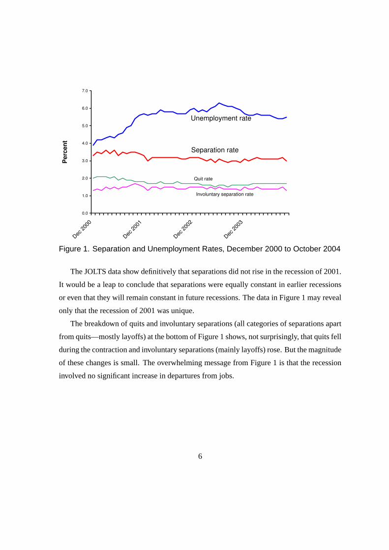
began in early 2001. Figure 1 shows the JOLTS separation rate and the standard unemploy-

ment rate from the Current Population Survey (CPS). The rise in unemployment through

2001 has no counterpart in higher separation rates. Rather, the separation rate fell a bit.

5

0.0

1.0

2.0

3.0

4.0

5.0

6.0

7.0

Dec

200

0

Dec

200

1

Dec

200

2

Dec

200

3

Pe

rc

en

t

Unemployment rate

Separation rate

Quit rate

Involuntary separation rate

Figure 1. Separation and Unemployment Rates, December 2000 to October 2004

The JOLTS data show definitively that separations did not rise in the recession of 2001.

It would be a leap to conclude that separations were equally constant in earlier recessions

or even that they will remain constant in future recessions. The data in Figure 1 may reveal

only that the recession of 2001 was unique.

The breakdown of quits and involuntary separations (all categories of separations apart

from quits—mostly layoffs) at the bottom of Figure 1 shows, not surprisingly, that quits fell

during the contraction and involuntary separations (mainly layoffs) rose. But the magnitude

of these changes is small. The overwhelming message from Figure 1 is that the recession

involved no significant increase in departures from jobs.

6

Industry

Average

monthly

separation

rate in

JOLTS

(percent)

Standard

deviation of

monthly

employment

change

(percent)

Standard

deviation of

annual

employment

change at

monthly rate

(percent)

Employment

share, 1990

(percent)

Natural resources and mining 3.17 1.79 0.59 0.7

Construction 5.76 1.04 0.43 5.0

Durable goods manufacturing 2.81 0.89 0.48 9.9

Nondurable goods manufacturing 2.90 0.36 0.21 6.4

Wholesale trade 2.53 0.27 0.17 4.8

Retail trade 4.39 0.37 0.16 12.1

Transportation, warehousing, and utilities 2.74 0.47 0.20 3.8

Information 2.37 1.72 0.32 2.4

Finance and insurance 1.85 0.18 0.14 4.6

Real estate and rental and leasing 3.10 0.22 0.12 1.5

Professional and business services 3.65 0.28 0.19 9.9

Educational services 1.79 0.40 0.19 1.5

Health care and social assistance 2.55 0.11 0.07 8.3

Arts, entertainment, and recreation 6.29 0.73 0.21 1.0

Accommodation and food services 6.26 0.24 0.11 7.5

Other services 3.18 0.22 0.14 3.9

Federal 1.23 1.10 0.32 2.8

State and local 1.23 0.27 0.16 13.8

Weighted average 3.23 0.69 0.26

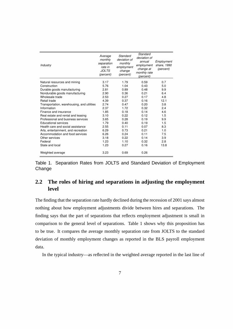
Table 1. Separation Rates from JOLTS and Standard Deviation of EmploymentChange

2.2 The roles of hiring and separations in adjusting the employmentlevel

The finding that the separation rate hardly declined during the recession of 2001 says almost

nothing about how employment adjustments divide between hires and separations. The

finding says that the part of separations that reflects employment adjustment is small in

comparison to the general level of separations. Table 1 shows why this proposition has

to be true. It compares the average monthly separation rate from JOLTS to the standard

deviation of monthly employment changes as reported in the BLS payroll employment

data.

In the typical industry—as reflected in the weighted average reported in the last line of

7

Table 1—more than three percent of workers depart employment each month. The standard

deviation of employment change, on the other hand, is only about 0.7 percent. Furthermore,

many of the larger monthly deviations are transitory, unlike the long sequence of declines

that occur in a recession. The standard deviation of employment changes over 12-month

spans, stated at monthly rates, is less than 0.3 percent. Even if all employment changes

occurred through changes in the separation rate and none through changes in hiring, the

changes in the separation rate would be close to invisible because of the high normal level

of separations.

Next I will present some results based on the hypothesis that JOLTS reveals behavior

that was stable over the period considered in this paper, 1948 to 2004. To generate a rough

approximation of separations for years before JOLTS, I regress the JOLTS separation rate

on industry employment-growth variables. Because an industry can expand rapidly only

by hiring and can contract rapidly only through separations, I include the positive part of

growth separately from the negative part.

I pooled the JOLTS data for the 18 industries listed in Table 1, jointly accounting for

all civilian employment, over the 46 available monthly observations. I used seasonally

unadjusted data for all variables (the BLS has not released seasonally adjusted data for

JOLTS at the industry level). The resulting estimate of the effect of negative industry

employment growth on separations is 0.29 with a standard error of 0.04 and the estimate

of the effect of positive industry growth is -0.05 with a standard error of 0.02. These

results confirm asymmetry in a reduced form sense, but they do not deserve structural

interpretations, because there is no reason to expect that the disturbance in the equation is

uncorrelated with employment growth. The equation serves only its intended purpose of

measuring the expectation of separations conditional on employment growth.

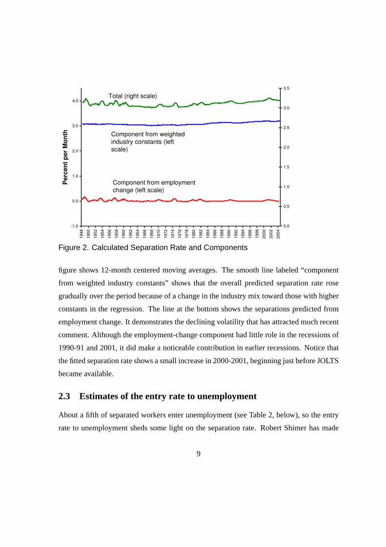
Figure 2 displays the fitted separations in terms of economy-wide aggregates, formed

by applying employment weights to the results by industry. I consolidate to the level of the

15 JOLTS industries that can be matched to payroll employment data back to 1948. The

8

-1.0

0.0

1.0

2.0

3.0

4.0

1948

1950

1952

1954

1956

1958

1960

1962

1964

1966

1968

1970

1972

1974

1976

1978

1980

1982

1984

1986

1988

1990

1992

1994

1996

1998

2000

2002

2004

Pe

rce

nt

pe

r M

on

th

0.0

0.5

1.0

1.5

2.0

2.5

3.0

3.5

Component from employment

change (left scale)

Component from weighted

industry constants (left

scale)

Total (right scale)

Figure 2. Calculated Separation Rate and Components

figure shows 12-month centered moving averages. The smooth line labeled “component

from weighted industry constants” shows that the overall predicted separation rate rose

gradually over the period because of a change in the industry mix toward those with higher

constants in the regression. The line at the bottom shows the separations predicted from

employment change. It demonstrates the declining volatility that has attracted much recent

comment. Although the employment-change component had little role in the recessions of

1990-91 and 2001, it did make a noticeable contribution in earlier recessions. Notice that

the fitted separation rate shows a small increase in 2000-2001, beginning just before JOLTS

became available.

2.3 Estimates of the entry rate to unemployment

About a fifth of separated workers enter unemployment (see Table 2, below), so the entry

rate to unemployment sheds some light on the separation rate. Robert Shimer has made

9

estimates of the entry rate from data from the Current Population Survey (Shimer (2005b)).

He concludes that there is little tendency for the rate to rise in recessions. He starts with

published data on total unemployment and on short-duration unemployment. The latter

serves as a measure of the flow into unemployment. His procedure pays close attention to

issues of time aggregation. The relation between the inflow to unemployment and the stock

of unemployed reveals the exit rate from unemployment—the flow probability of leaving

unemployment by finding work or leaving the labor force. From the stock of unemployment

and his calculated exit rate, he infers the entry rate.

The entry rate to unemployment measures the separation rate from employment if ev-

ery worker leaving a job becomes unemployed and if everybody becoming unemployed

was previously employed. Neither of these holds even as a first approximation. Transi-

tions from jobs to new jobs without intervening unemployment are common and so are

transitions from employment to out of the labor force and from out of the labor force to

unemployment. Shimer (2005c) shows that the flow from employment to out of the labor

force is not cyclical, though it has sub-cyclical trends. He also shows that the flow from

out of the labor force to unemployment rises slightly in recessions, so removing it from his

measure of separations would strengthen his finding that the separation rate does not rise in

recessions. Finally, he shows that, during the time since the CPS was revised to include the

relevant question, job-to-job transitions fell during the one observed recession, in 2001.

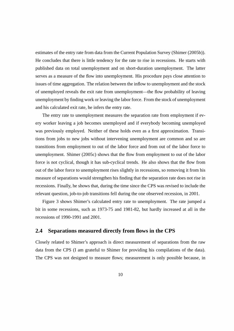
Figure 3 shows Shimer’s calculated entry rate to unemployment. The rate jumped a

bit in some recessions, such as 1973-75 and 1981-82, but hardly increased at all in the

recessions of 1990-1991 and 2001.

2.4 Separations measured directly from flows in the CPS

Closely related to Shimer’s approach is direct measurement of separations from the raw

data from the CPS (I am grateful to Shimer for providing his compilations of the data).

The CPS was not designed to measure flows; measurement is only possible because, in

10

0

1

2

3

4

5

6

1948 1951 1954 1957 1960 1963 1966 1969 1972 1975 1978 1981 1984 1987 1990 1993 1996 1999 2002

Ra

te, p

erc

en

t

Figure 3. Shimer’s Unemployment Entry Rate Calculated from the CPS

most months, one can match data for people reported in that month to data reported in

the previous month. Flows are inferred from differences in status reported in consecutive

months. As a result, random errors in measuring status raise the levels of the flows. This

problem has impeded research on labor-market dynamics based on the CPS. Longitudinal

data overcome the problem—I discuss one important longitudinal survey below.

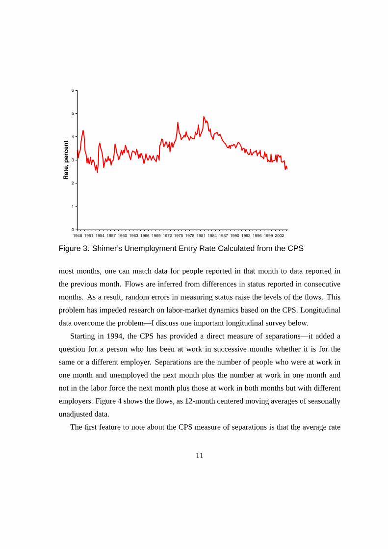
Starting in 1994, the CPS has provided a direct measure of separations—it added a

question for a person who has been at work in successive months whether it is for the

same or a different employer. Separations are the number of people who were at work in

one month and unemployed the next month plus the number at work in one month and

not in the labor force the next month plus those at work in both months but with different

employers. Figure 4 shows the flows, as 12-month centered moving averages of seasonally

unadjusted data.

The first feature to note about the CPS measure of separations is that the average rate

11

0

1

2

3

4

5

6

7

8

1994 1995 1996 1997 1998 1999 2000 2001 2002 2003

Ra

te, p

erc

en

t p

er

mo

nth

Employment to Unemployment

Employment to New Job

Employment to out of Labor Force

Total Separation Rate

Figure 4. Separation Rate Measured in the CPS, 1994-2004

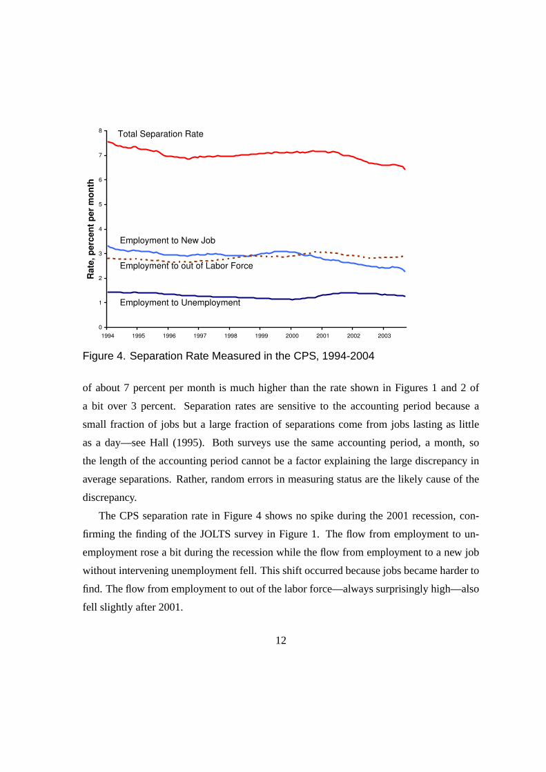
of about 7 percent per month is much higher than the rate shown in Figures 1 and 2 of

a bit over 3 percent. Separation rates are sensitive to the accounting period because a

small fraction of jobs but a large fraction of separations come from jobs lasting as little

as a day—see Hall (1995). Both surveys use the same accounting period, a month, so

the length of the accounting period cannot be a factor explaining the large discrepancy in

average separations. Rather, random errors in measuring status are the likely cause of the

discrepancy.

The CPS separation rate in Figure 4 shows no spike during the 2001 recession, con-

firming the finding of the JOLTS survey in Figure 1. The flow from employment to un-

employment rose a bit during the recession while the flow from employment to a new job

without intervening unemployment fell. This shift occurred because jobs became harder to

find. The flow from employment to out of the labor force—always surprisingly high—also

fell slightly after 2001.

12

0

1

2

3

4

5

6

1967

1968

1969

1970

1971

1972

1973

1974

1975

1976

1977

1978

1979

1980

1981

1982

1983

1984

1985

1986

1987

1988

1989

1990

1991

1992

1993

1994

1995

1996

1997

1998

1999

2000

2001

2002

2003

Ra

te, p

erc

en

t p

er

mo

nth

Employment to Unemployment

Employment to out of Labor Force

Sum

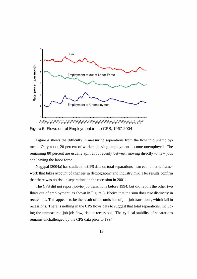
Figure 5. Flows out of Employment in the CPS, 1967-2004

Figure 4 shows the difficulty in measuring separations from the flow into unemploy-

ment. Only about 20 percent of workers leaving employment become unemployed. The

remaining 80 percent are usually split about evenly between moving directly to new jobs

and leaving the labor force.

Nagypal (2004a) has studied the CPS data on total separations in an econometric frame-

work that takes account of changes in demographic and industry mix. Her results confirm

that there was no rise in separations in the recession in 2001.

The CPS did not report job-to-job transitions before 1994, but did report the other two

flows out of employment, as shown in Figure 5. Notice that the sum does rise distinctly in

recessions. This appears to be the result of the omission of job-job transitions, which fall in

recessions. There is nothing in the CPS flows data to suggest that total separations, includ-

ing the unmeasured job-job flow, rise in recessions. The cyclical stability of separations

remains unchallenged by the CPS data prior to 1994.

13

0.02

0.03

0.04

0.05

0.06

83 84 85 86 87 88 89 90 91 92 93 94 95

Year

Job E

xit R

ate

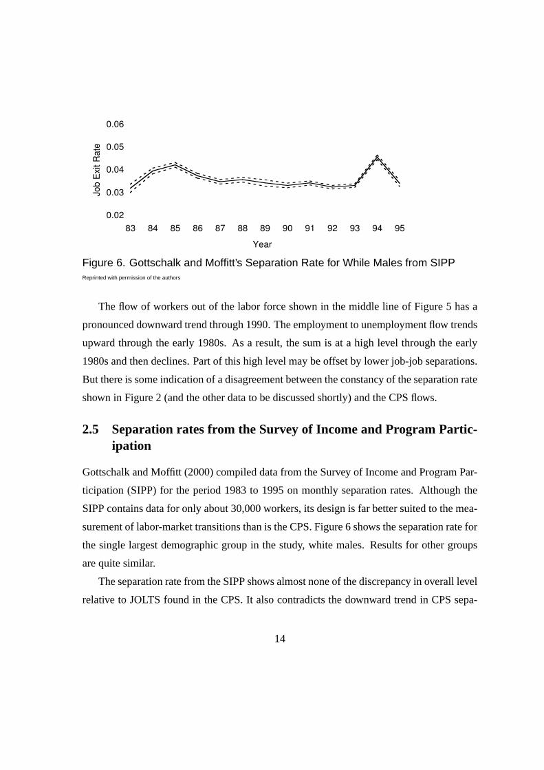
Figure 6. Gottschalk and Moffitt’s Separation Rate for While Males from SIPPReprinted with permission of the authors

The flow of workers out of the labor force shown in the middle line of Figure 5 has a

pronounced downward trend through 1990. The employment to unemployment flow trends

upward through the early 1980s. As a result, the sum is at a high level through the early

1980s and then declines. Part of this high level may be offset by lower job-job separations.

But there is some indication of a disagreement between the constancy of the separation rate

shown in Figure 2 (and the other data to be discussed shortly) and the CPS flows.

2.5 Separation rates from the Survey of Income and Program Partic-ipation

Gottschalk and Moffitt (2000) compiled data from the Survey of Income and Program Par-

ticipation (SIPP) for the period 1983 to 1995 on monthly separation rates. Although the

SIPP contains data for only about 30,000 workers, its design is far better suited to the mea-

surement of labor-market transitions than is the CPS. Figure 6 shows the separation rate for

the single largest demographic group in the study, white males. Results for other groups

are quite similar.

The separation rate from the SIPP shows almost none of the discrepancy in overall level

relative to JOLTS found in the CPS. It also contradicts the downward trend in CPS sepa-

14

rations in Figure 4. Except for bulges in 1985 and 1994, the SIPP separation rate supports

the hypothesis of constant separations. These bulges—both in years of high employment

growth when separations should be slightly lower, according to the earlier results—have no

obvious explanation.

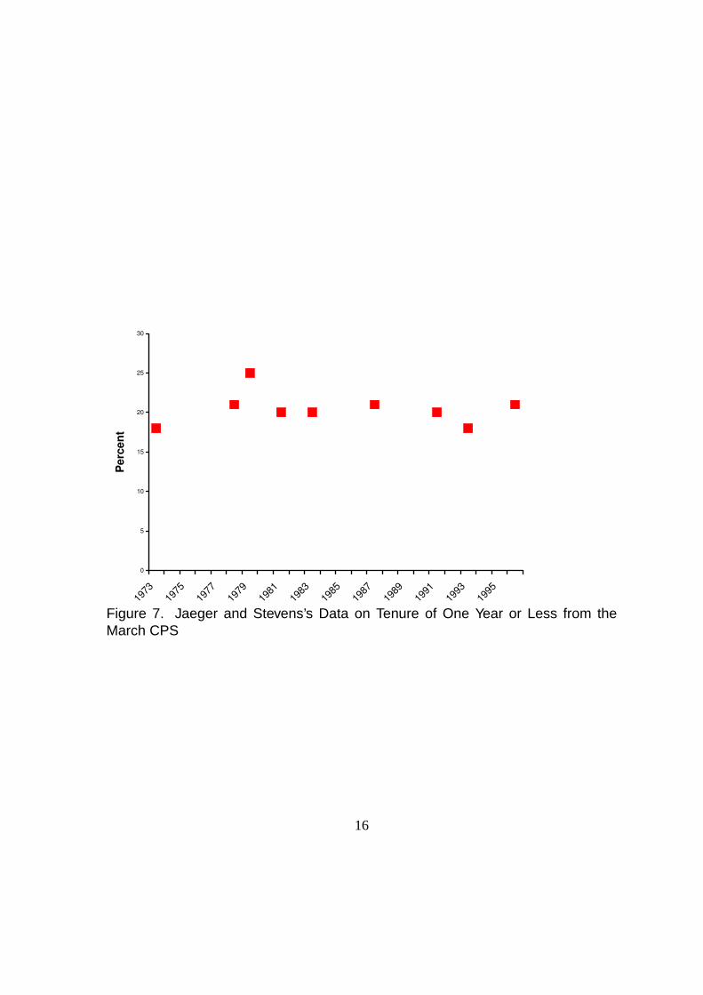
2.6 Separation rates inferred from data on job tenure

Another useful source of information is a question about tenure that has appeared every few

years in the March CPS. The fraction of workers who started work recently is a measure

of the hiring rate. As noted earlier, differences between the hiring rate and the separation

are tiny, so the tenure data come close to revealing the separation rate. Although the CPS

records tenure in months if it is one year or less, I have not found a tabulation of the data

that reports the one-month figure separately, which is the measure most comparable to the

others I consider in this paper. Jaeger and Stevens (2000) tabulate fraction of workers with

tenure of one year or less, as shown in Figure 7. Higher monthly separation rates would

result in higher fractions of workers with short tenure. Except the one high figure in 1979,

the low-tenure fraction is close to constant. Again, I find support for the view that the

separation rate has been constant over past decades, despite the higher apparent rate in the

CPS data.

Much additional research could be done on this point with existing sources. My tenta-

tive conclusion is that a constant separation rate is the best approximation over past decades.

But this conclusion comes from examining a number of sources, each of which shows

movement over the period, and finding that the movements are not correlated. The evi-

dence is not strong. And, of course, the constancy of the separation rate in Figure 2 is

virtually an assumption and should not be taken as confirmation of constancy.

2.7 Relation between separations and job destruction

Davis and Haltiwanger (1992) introduced the concept of job destruction to labor turnover

15

0

5

10

15

20

25

30

1973

1975

1977

1979

1981

1983

1985

1987

1989

1991

1993

1995

Pe

rc

en

t

Figure 7. Jaeger and Stevens’s Data on Tenure of One Year or Less from theMarch CPS

16

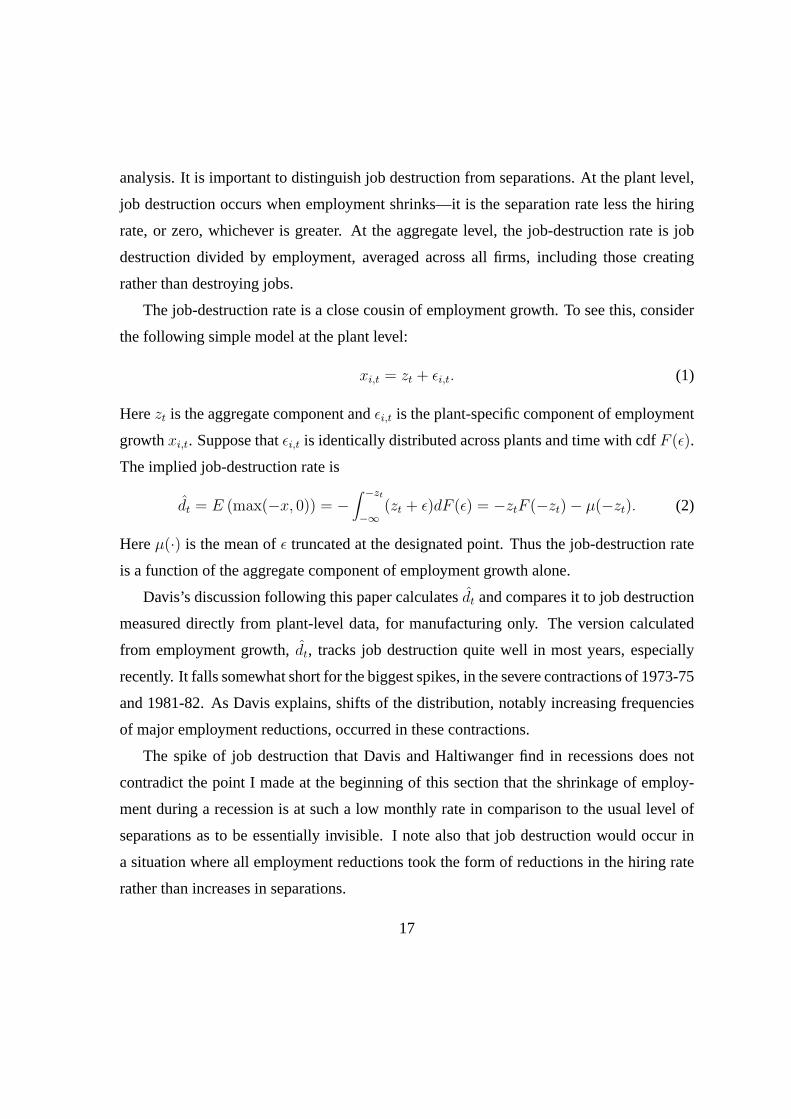
analysis. It is important to distinguish job destruction from separations. At the plant level,

job destruction occurs when employment shrinks—it is the separation rate less the hiring

rate, or zero, whichever is greater. At the aggregate level, the job-destruction rate is job

destruction divided by employment, averaged across all firms, including those creating

rather than destroying jobs.

The job-destruction rate is a close cousin of employment growth. To see this, consider

the following simple model at the plant level:

xi,t = zt + εi,t. (1)

Herezt is the aggregate component andεi,t is the plant-specific component of employment

growthxi,t. Suppose thatεi,t is identically distributed across plants and time with cdfF (ε).

The implied job-destruction rate is

dt = E (max(−x, 0)) = −∫ −zt

−∞(zt + ε)dF (ε) = −ztF (−zt)− µ(−zt). (2)

Hereµ(·) is the mean ofε truncated at the designated point. Thus the job-destruction rate

is a function of the aggregate component of employment growth alone.

Davis’s discussion following this paper calculatesdt and compares it to job destruction

measured directly from plant-level data, for manufacturing only. The version calculated

from employment growth,dt, tracks job destruction quite well in most years, especially

recently. It falls somewhat short for the biggest spikes, in the severe contractions of 1973-75

and 1981-82. As Davis explains, shifts of the distribution, notably increasing frequencies

of major employment reductions, occurred in these contractions.

The spike of job destruction that Davis and Haltiwanger find in recessions does not

contradict the point I made at the beginning of this section that the shrinkage of employ-

ment during a recession is at such a low monthly rate in comparison to the usual level of

separations as to be essentially invisible. I note also that job destruction would occur in

a situation where all employment reductions took the form of reductions in the hiring rate

rather than increases in separations.

17

3 Unemployment and the Job-Finding Rate

Because the separation rate is close to constant—or at least does not rise in recessions—all

of the burden of explaining fluctuations in the unemployment rate falls on variations in the

rate that job-seekers find jobs. But there are many ways to measure the job-finding rate.

As the CPS flows data demonstrate, workers often change jobs without visible intervening

unemployment. Thus there is a job-finding rate for job-holders. People often take jobs after

having been out of the labor force, so there is a job-finding rate for that group. And the

job-finding rate for the unemployed is a third important concept.

A job-finding rate is the ratio of the flow from another activity into employment, divided

by the number of people seeking to find jobs. Finding the denominator for any job-finding

rate is a challenge. Only a minority of the employed are looking for work—most have

sufficiently strong comparative advantages in their current jobs so that the likelihood of

finding better jobs is small. A job-finding rate for the employed that took total employment

as the denominator would fail to record any significant changes, given the constancy of the

numerator.

Finding a denominator for those out of the labor force encounters the same obstacles.

Most people not working or looking for work have a strong comparative advantage in some

non-work activity, so they are not looking for work.

To deal with this issue, I proceed in the following way. First, I do not attempt to measure

a job-finding rate for the employed. I believe that the rate based on a denominator that omits

employed job-seekers is the best available measure. When it is hard for the unemployed

or those out of the labor force to find jobs, it is surely likely to be just as hard for those

thinking of leaving existing jobs to find new jobs. This relation is an implication of the

various recent models incorporating on-the-job search discussed in a later section.

Second, I consider a measure of unemployment expanded to include people who are are

classified as out of the labor force in a given month, but are likely to move into the labor

force soon. The improvements in the CPS introduced in 1994 included questions that iden-

18

Not in

labor

force

Unem-

ployed Working

Not in labor

force 92.8 22.7 3.2

Unemployed 2.5 49.6 1.5Working 4.7 27.6 95.4

From

To

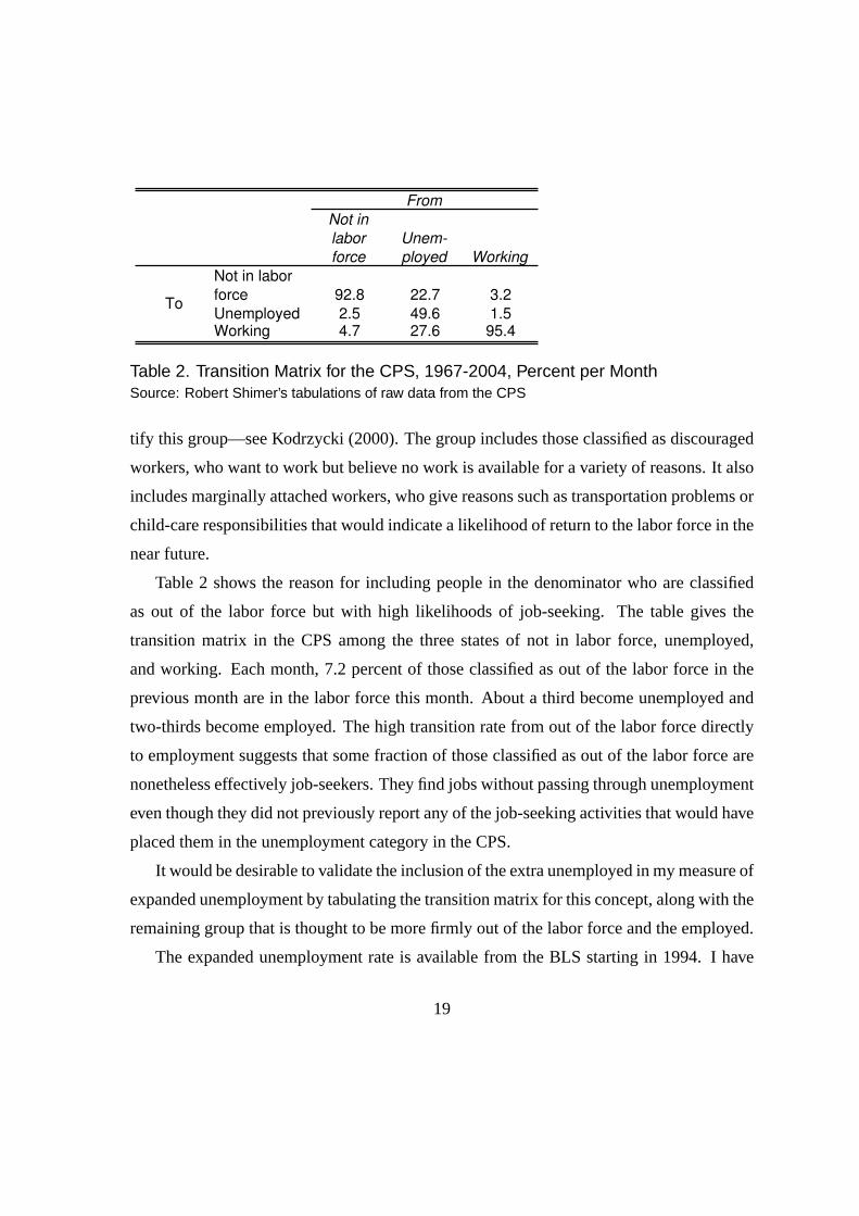
Table 2. Transition Matrix for the CPS, 1967-2004, Percent per MonthSource: Robert Shimer’s tabulations of raw data from the CPS

tify this group—see Kodrzycki (2000). The group includes those classified as discouraged

workers, who want to work but believe no work is available for a variety of reasons. It also

includes marginally attached workers, who give reasons such as transportation problems or

child-care responsibilities that would indicate a likelihood of return to the labor force in the

near future.

Table 2 shows the reason for including people in the denominator who are classified

as out of the labor force but with high likelihoods of job-seeking. The table gives the

transition matrix in the CPS among the three states of not in labor force, unemployed,

and working. Each month, 7.2 percent of those classified as out of the labor force in the

previous month are in the labor force this month. About a third become unemployed and

two-thirds become employed. The high transition rate from out of the labor force directly

to employment suggests that some fraction of those classified as out of the labor force are

nonetheless effectively job-seekers. They find jobs without passing through unemployment

even though they did not previously report any of the job-seeking activities that would have

placed them in the unemployment category in the CPS.

It would be desirable to validate the inclusion of the extra unemployed in my measure of

expanded unemployment by tabulating the transition matrix for this concept, along with the

remaining group that is thought to be more firmly out of the labor force and the employed.

The expanded unemployment rate is available from the BLS starting in 1994. I have

19

0

2

4

6

8

10

12

14

16

18

20

u

Ra

te, p

erc

en

t

Imputed Actual

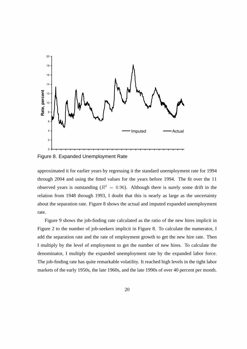
Figure 8. Expanded Unemployment Rate

approximated it for earlier years by regressing it the standard unemployment rate for 1994

through 2004 and using the fitted values for the years before 1994. The fit over the 11

observed years is outstanding (R2 = 0.96). Although there is surely some drift in the

relation from 1948 through 1993, I doubt that this is nearly as large as the uncertainty

about the separation rate. Figure 8 shows the actual and imputed expanded unemployment

rate.

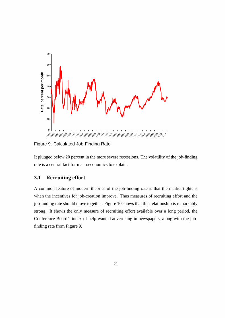
Figure 9 shows the job-finding rate calculated as the ratio of the new hires implicit in

Figure 2 to the number of job-seekers implicit in Figure 8. To calculate the numerator, I

add the separation rate and the rate of employment growth to get the new hire rate. Then

I multiply by the level of employment to get the number of new hires. To calculate the

denominator, I multiply the expanded unemployment rate by the expanded labor force.

The job-finding rate has quite remarkable volatility. It reached high levels in the tight labor

markets of the early 1950s, the late 1960s, and the late 1990s of over 40 percent per month.

20

0

10

20

30

40

50

60

70

1948

1950

1952

1954

1956

1958

1960

1962

1964

1966

1968

1970

1972

1974

1976

1978

1980

1982

1984

1986

1988

1990

1992

1994

1996

1998

2000

2002

2004

Ra

te, p

erc

en

t p

er

mo

nth

Figure 9. Calculated Job-Finding Rate

It plunged below 20 percent in the more severe recessions. The volatility of the job-finding

rate is a central fact for macroeconomics to explain.

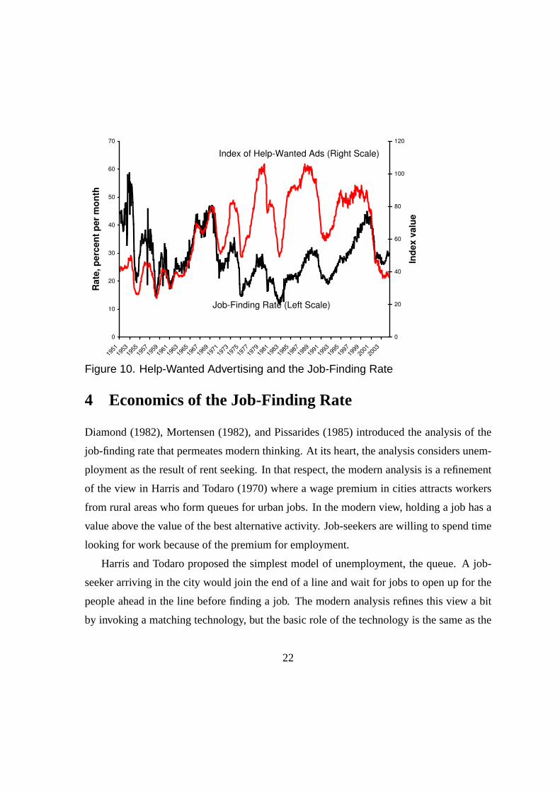
3.1 Recruiting effort

A common feature of modern theories of the job-finding rate is that the market tightens

when the incentives for job-creation improve. Thus measures of recruiting effort and the

job-finding rate should move together. Figure 10 shows that this relationship is remarkably

strong. It shows the only measure of recruiting effort available over a long period, the

Conference Board’s index of help-wanted advertising in newspapers, along with the job-

finding rate from Figure 9.

21

0

10

20

30

40

50

60

70

1951

1953

1955

1957

1959

1961

1963

1965

1967

1969

1971

1973

1975

1977

1979

1981

1983

1985

1987

1989

1991

1993

1995

1997

1999

2001

2003

Ra

te, p

erc

en

t p

er

mo

nth

0

20

40

60

80

100

120

Ind

ex v

alu

e

Job-Finding Rate (Left Scale)

Index of Help-Wanted Ads (Right Scale)

Figure 10. Help-Wanted Advertising and the Job-Finding Rate

4 Economics of the Job-Finding Rate

Diamond (1982), Mortensen (1982), and Pissarides (1985) introduced the analysis of the

job-finding rate that permeates modern thinking. At its heart, the analysis considers unem-

ployment as the result of rent seeking. In that respect, the modern analysis is a refinement

of the view in Harris and Todaro (1970) where a wage premium in cities attracts workers

from rural areas who form queues for urban jobs. In the modern view, holding a job has a

value above the value of the best alternative activity. Job-seekers are willing to spend time

looking for work because of the premium for employment.

Harris and Todaro proposed the simplest model of unemployment, the queue. A job-

seeker arriving in the city would join the end of a line and wait for jobs to open up for the

people ahead in the line before finding a job. The modern analysis refines this view a bit

by invoking a matching technology, but the basic role of the technology is the same as the

22

role of the queue in Harris-Todaro.

The value that attracts job-seekers depends on the wage that workers receive upon em-

ployment. Thus a critical piece of the theory of the job-finding rate is the model of wage

determination. Until recently, the standard model was the Nash bargain. The worker’s

threat point is to continue searching rather than work for a candidate employer and the em-

ployer’s threat point is to deny the worker employment. The wage bargain places the parties

on a point partway between the threat points. To put it differently, the two parties have a

joint surplus, equal to the joint value they achieve from a match less their values at the

threat points. The Nash bargain splits the surplus between the parties in given proportions.

The standard setup includes a theory of separations, implicit in the wage-bargain model.

If the surplus of an existing match becomes negative, the parties will split up and a separa-

tion will occur. Because separations are not actually variable and because models with en-

dogenous separations have other unrealistic implications, many models assume a fixed ex-

ogenous probability of separation, viewed as a probability that the productivity of a match

will plunge to zero and make the separation inevitable.

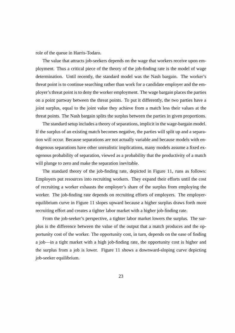
The standard theory of the job-finding rate, depicted in Figure 11, runs as follows:

Employers put resources into recruiting workers. They expand their efforts until the cost

of recruiting a worker exhausts the employer’s share of the surplus from employing the

worker. The job-finding rate depends on recruiting efforts of employers. The employer-

equilibrium curve in Figure 11 slopes upward because a higher surplus draws forth more

recruiting effort and creates a tighter labor market with a higher job-finding rate.

From the job-seeker’s perspective, a tighter labor market lowers the surplus. The sur-

plus is the difference between the value of the output that a match produces and the op-

portunity cost of the worker. The opportunity cost, in turn, depends on the ease of finding

a job—in a tight market with a high job-finding rate, the opportunity cost is higher and

the surplus from a job is lower. Figure 11 shows a downward-sloping curve depicting

job-seeker equilibrium.

23

Job-finding rate

Su

rplu

s

Employer equilibrium

Job-seeker equilibrium

Figure 11. Equilibrium in the Standard Model

The equilibrium of the labor market occurs at the intersection of the two curves. Notice

the key role of the Nash-bargain model of wage determination. The employer-equilibrium

curve deals with the employer’s share of the surplus and the job-seeker-equilibrium with

the job-seeker’s share. The Nash assumption locks the two together.

The dashed line in Figure 11 shows the effect of a three-percent decline in productivity.

The job-seeker-equilibrium curve shifts downward slightly, the job-finding rate drops a

little, and unemployment rises a bit. No shift occurs in the employer-equilibrium curve.

The shift in the job-seeker curve is small for the following reason: The surplus is the

difference between the present value of a worker’s product and the worker’s opportunity

cost. The opportunity cost depends mainly on the wage that would be paid by alternative

jobs. Under the Nash assumption, that wage falls almost as much as does productivity. The

surplus hardly changes. Shimer (2005a) was the first to make this observation.

The finding of limited response of unemployment to changes in productivity suggests

that the standard theory is not a satisfactory account of fluctuations in unemployment. In the

24

typical recession, unemployment rises by several percentage points and remains high for

several years. No conceivable movement of productivity, when fed into the standard model,

could replicate the observed movements of unemployment in recessions. Shimer’s paper

set off a quest for alternative models that could explain the high volatility of unemployment.

Mortensen (2005) and Hagedorn and Manovskii (2005) observe that Shimer’s result is

not universal—it rests on an assumption about labor supply. Shimer and I belong to the

school of macroeconomics that believes that alternative activities for most workers, includ-

ing unemployment compensation, are worth far less than the workers produce on the job.

The elasticity of labor supply is low. The fundamental driving force of the standard model

is the difference between productivity and the value of non-work. A given change in pro-

ductivity has a larger proportional effect on that difference if the value of non-work is close

to the level of productivity. The standard model can generate high levels of unemployment

volatility by setting the value of non-work only a bit below the level of productivity. The

rest of my discussion is for the benefit of readers who share Shimer’s and my belief in

relatively inelastic labor supply.

5 Alternative Views of Wage Determination

Much of the effort focusing on creating a modern theory of unemployment fluctuations

replaces the Nash bargain with some other model of wage determination.

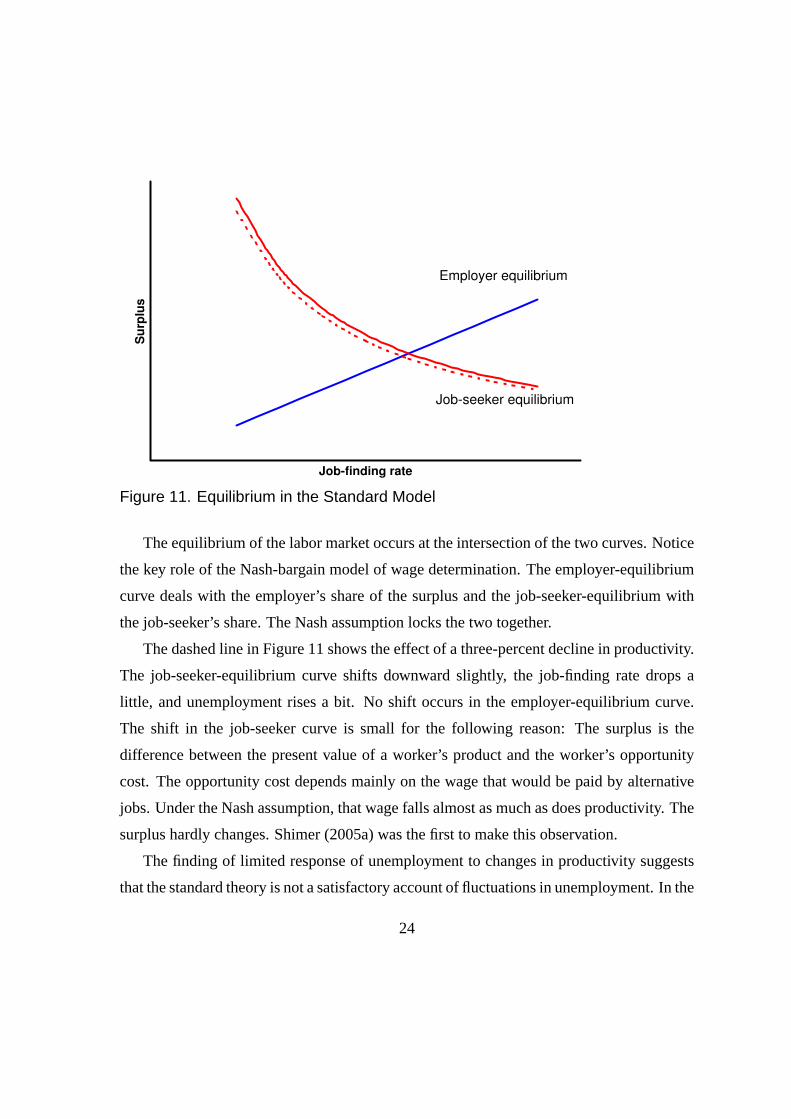
5.1 Fixed wage

Job-finding and unemployment are highly sensitive to productivity if the standard model

is altered in just one way, by keeping the wage fixed and unresponsive to changes in

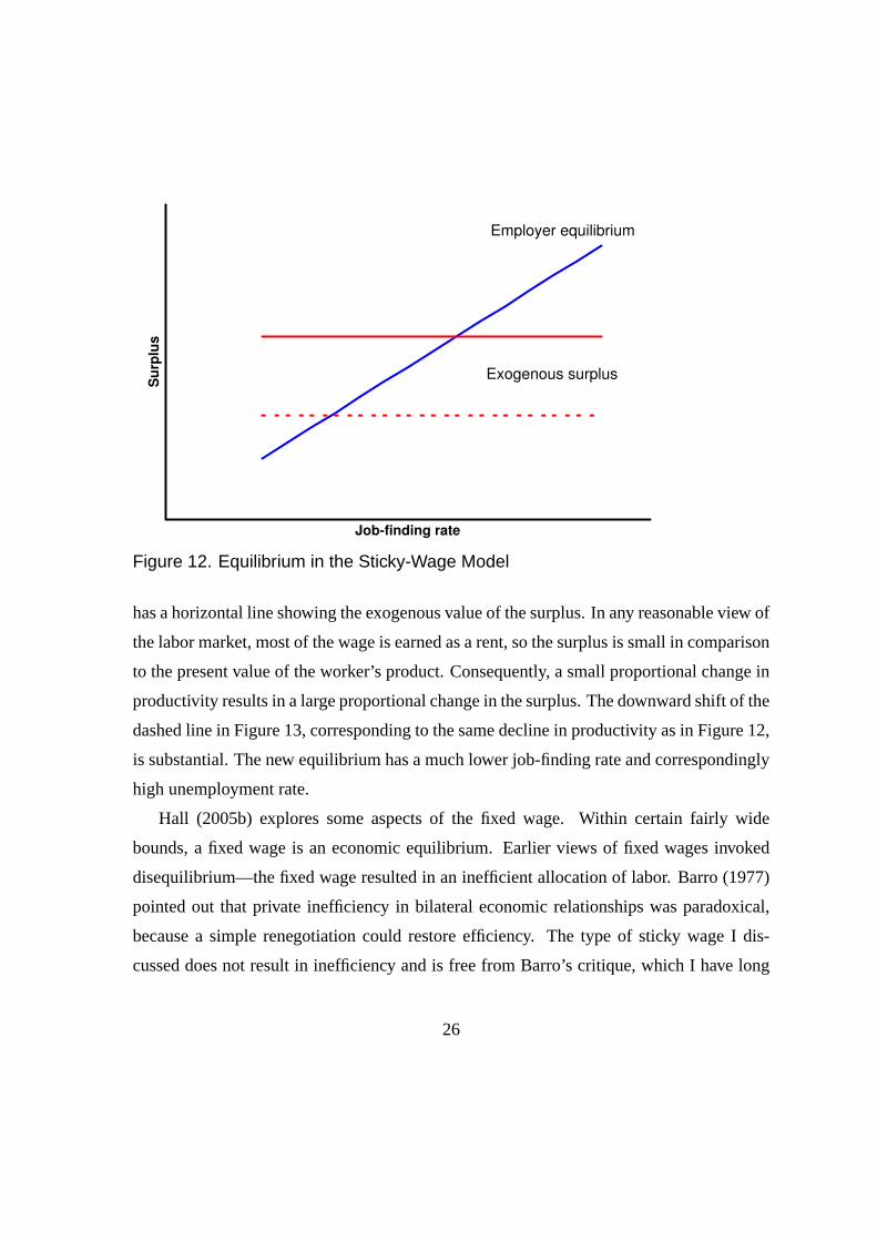
productivity—see Shimer (2004). Figure 13 shows why. If the wage is fixed, the sur-

plus received by the employer is the difference between the present value of the worker’s

product and the fixed wage. The employer-equilibrium curve is unaffected, but job-seeker

equilibrium no longer plays a role in determining the job-finding rate. Instead, the diagram

25

Job-finding rate

Su

rplu

s

Employer equilibrium

Exogenous surplus

Figure 12. Equilibrium in the Sticky-Wage Model

has a horizontal line showing the exogenous value of the surplus. In any reasonable view of

the labor market, most of the wage is earned as a rent, so the surplus is small in comparison

to the present value of the worker’s product. Consequently, a small proportional change in

productivity results in a large proportional change in the surplus. The downward shift of the

dashed line in Figure 13, corresponding to the same decline in productivity as in Figure 12,

is substantial. The new equilibrium has a much lower job-finding rate and correspondingly

high unemployment rate.

Hall (2005b) explores some aspects of the fixed wage. Within certain fairly wide

bounds, a fixed wage is an economic equilibrium. Earlier views of fixed wages invoked

disequilibrium—the fixed wage resulted in an inefficient allocation of labor. Barro (1977)

pointed out that private inefficiency in bilateral economic relationships was paradoxical,

because a simple renegotiation could restore efficiency. The type of sticky wage I dis-

cussed does not result in inefficiency and is free from Barro’s critique, which I have long

26

found utterly persuasive. In a matching model, the joint surplus measures the width of

the bargaining set for the wage. A sticky wage remains efficient as long as it is within

the bargaining set. I derive conditions under which a sticky wage remains within the bar-

gaining set, even though the boundaries of the set fluctuate along with productivity. These

conditions are not very restrictive.

As not a single reader of Hall (2005b) has failed to point out, the demonstration that a

sticky wage is an equilibrium is far from an explanation for stickiness. Many other patterns

of wage movement are equilibria, including ones that are more volatile than the Nash wage

and result in increases in unemployment when productivity falls. I do try to connect wage

inertia with the idea of a social norm. Still, the primary reason that the sticky-wage case is

interesting is the general impression that wages are, in fact, quite sticky.

The paper also makes the point that wages can be sticky relative to an index that grows

over time. The result is a more sophisticated model of wage inertia, similar to the model

implicit in many discussions of the Phillips curve and monetary non-neutrality.

Gertler and Trigari (2005) develop another version of the equilibrium sticky-wage model.

Employers and workers make a standard Nash bargain that last many periods. Workers

hired between wage bargaining episodes receive the previously bargained wage. This setup

delivers the essential feature of the equilibrium sticky-wage model—the sensitivity of the

employer’s gain from a new hire to current economic conditions. The wage does not re-

spond immediately to those conditions. Unemployment is sensitive to driving forces until

the next wage bargain. The persistence of unemployment fluctuations depends on the du-

ration of wage bargains.

5.2 Kennan’s model

Kennan (2005) considers the standard model with the following alternative model of wage

determination: Upon forming a candidate match, the parties toss a coin to decide who will

make an offer to the other. If the employer wins the toss, the employer offers the job-

27

seeker her reservation wage. If the winner, the job-seeker has a more complicated decision,

because the job-seeker’s productivity is known to the employer but is hidden from the job-

seeker. The job-seeker is in the same position as a bidder in a first-price sealed-bid auction.

Kennan makes assumptions that cause the job-seeker to bid a wage that is insensitive to

current conditions. Thus he reaches a sticky-wage property as a derived conclusion rather

than as a bald assumption, a step forward. Kennan’s model delivers a high sensitivity of

unemployment to changes in productivity for the reasons shown in Figure 12.

The sticky-wage conclusion is a special feature of the setup of his model. The hidden

information is binary—match productivity is either high or low. The job-seeker knows the

two values but does not know which one holds. Kennan assumes an environment where

the job-seeker always picks the lower value, thus guaranteeing employment but giving

the employer a large part of the surplus when the realization is the higher value of match

productivity. Increases in aggregate productivity take the form of a higher probability of

the better level of match productivity, but not enough higher to cause any job-seeker to bid

higher. Thus a sticky wage is essentially built into the model.

In a more general version of the model, the job-seeker knows that match productivity

can take on many values or is a continuous random variable. In that case, the job-seeker

will make a higher bid when conditions are better, using the general principles of first-price

auction theory. In another variant of this type of model, the wage might be determined by

a different procedure, such as a double auction where both employer and job-seeker make

bids. Tawara (2005) generalizes wage determination in Kennan’s model.

Kennan’s emphasis on informational rents that vary over time is an important contribu-

tion to the theory of fluctuations in the job-finding rate. When rents earned by employers

are high, firms will invest more heavily in recruitment efforts and the market will tighten,

with higher job-finding rates. Further work in this area may demonstrate that variation in

informational rents might plausibly be large enough to explain observed fluctuations. It

needs to elucidate how the exogenous events that trigger recessions cause reductions in

28

rents and thus bring higher unemployment.

5.3 Reconsideration of the threat points in the wage bargain

Hall and Milgrom (2005) point out that the threat points considered in the standard labor-

market bargaining model are not credible. Once a qualified worker and an employer have

met and found that they would enjoy a joint surplus, the threats to disclaim the match are

hollow. The sequential bargaining framework of Binmore, Rubinstein and Wolinsky (1986)

considers alternative, credible threats. The parties alternate in making wage proposals to

each other. The threat point of each is to prolong bargaining by declining an offer and

making a counteroffer. Each understands the implications of the process, so the unique

equilibrium is an immediate Nash-type bargain in which the threat points are the payoffs to

delaying indefinitely.

Changing the standard model in only one respect—changing the threat points to the

payoffs to endless delay—has a profound effect. The wage becomes fully insulated from

conditions in the labor market, such as unemployment. The wage does respond to produc-

tivity, but only half as much as in the standard model. The result is a strong response of

unemployment to productivity and other driving forces. The wage no longer has an equili-

brating role. If productivity falls, the part of the surplus accruing to employers falls sharply

and they cut back on recruiting effort. The labor market softens dramatically.

We also consider two variants in which the wage is more closely connected to unem-

ployment, though not as strongly as in the standard model. First, we alter the matching

framework so that, part of the time, more than one applicant bargains with an employer for

a job opening. If there is a single applicant, the parties engage in the bargaining process

just described. If there are more applicants, they engage in Bertrand competition for the

opening and one of them winds up with the job, but is only paid his reservation wage. The

employer gains all of the surplus. Because the likelihood of competition is greater in a soft

labor market, recruiting effort equilibrates the market more aggressively with this modifi-

29

cation. Nonetheless, the model delivers a higher response of unemployment to productivity

and other fluctuations than does the standard model.

In the second variant, there is a small probability that a worker will take another job

during the process of bargaining with a prospective employer. Again, this modification

links the wage to conditions in the labor market, but does not completely undo the effect of

using credible threat points in the basic wage-bargaining model.

6 Models that Explain Job-Finding Volatility with Flexi-ble Wages

Research has been active recently in trying to meet the challenge of Shimer (2005a) without

invoking sticky wages directly. In some cases, low wage volatility is a conclusion derived

from the fundamentals.

6.1 Models with on-the-job search

Figure 3 shows that the job-to-job flow accounts for almost half of all separations in normal

times. No theory of labor-market dynamics could possibly be complete without consider-

ation of this key flow. Many job-seekers are recorded as employed, not unemployed. A

number authors have created models with on-the-job search—one of the most prominent is

Burdett and Mortensen (1998). Prior to the search for amplification mechanisms launched

by Shimer, these models tended to deliver even less job-finding volatility than did the basic

Mortensen-Pissarides model—see Nagypal (2004b).

Nagypal combines on-the-job search with a number of other key ingredients to achieve

quite substantial amplification relative to the Mortensen-Pissarides model where workers

search only after losing jobs. First, employers need to prefer recruiting people directly out

of other jobs rather than from the unemployed. In the standard model, employers have

the opposite preference because the likelihood of forming a match with a candidate who is

30

unemployed is higher than with a candidate who has a job. The latter has a higher reser-

vation wage. In a recession, when the mix of job-seekers shifts towards the unemployed,

employers intensify recruiting efforts on account of the more favorable mix. This factor

results in the attenuation of the already low response of the job-finding rate to changes in

productivity.

To reverse this effect, Nagypal introduces heterogeneity in job matches. Workers have

different satisfaction levels with their jobs, hidden from employers. Workers hired from

unemployment are less desirable because those who form matches will have a lower aver-

age job satisfaction. They are more likely to leave the job soon as they search for better

jobs while employed. The final key element is a fixed cost of training a new worker. A quit

deprives the employer of the value of the training cost. Nagypal suggests that it is plausible

that the costs from the higher turnover of workers hired from the unemployed considerably

more than offsets the easier recruitment of the unemployed.

If the offset is strong enough, the mix effect goes in the opposite direction from earlier

models with on-the-job search. In Nagypal’s calibration, the elasticity of the unemployment

rate with respect to productivity is about−5. A decline of productivity of one percent raises

the unemployment rate by about 0.3 percentage points. Although this is quite a bit more

than in the standard model, it still requires implausibly large shocks to explain the increase

in unemployment of two or three percentage points in the typical recession.

Krause and Lubik (2004), working independently from Nagypal, present a different

model of amplification from on-the-job search. Their model permits variations in the in-

tensity of on-the job-search, a feature also present in Nagypal’s. Search effort of workers

intending to move directly to better jobs is highly elastic. When a persistent but ultimately

temporary productivity shock hits the economy, the stock of workers who find it newly

desirable to look for higher-wage jobs rises. During the fairly long period before these

workers actually move, wages do not rise as much as productivity. The surplus available

to employers—the difference between productivity and the wage—remains high for an

31

extended period. Through the standard mechanism of the Mortensen-Pissarides class of

models, the higher surplus to employer stimulates recruiting effort and tightens the labor

market. Endogenous wage stickiness delivers a result in their model similar to the one

reported for exogenous wage stickiness in Shimer (2005a).

The Krause-Lubik view calls for high volatility of job-job flows. They show that quits

as recorded in the old manufacturing turnover survey were quite volatile, but do not mention

the direct measure of the job-job flow shown in Figure 2. In their model, as the market

tightened from slack conditions in 1994 to extremely tight conditions in 2000, the job-job

flow should have risen. Instead, it fell a small amount.

6.2 Shimer and Wright’s model with hidden information and hiddenaction

Shimer and Wright (2004) develop a model of the labor market featuring numerous sub-

markets. All the employers in a sub-market offer the same contingent employment contract

to workers who choose to enter the sub-market. Workers know the terms of the contracts

in all of the sub-markets and pick the sub-market offering the most favorable contract.

Having chosen a sub-market, the job-seeker encounters a standard matching technology

which delivers a flow probability of meeting an employer and entering into a contract.

The contracting problem has an action hidden from employers—the investment that the

worker makes in establishing the relationship—and information hidden from workers—the

productivity of the resulting match. The contract needs to provide an incentive for the

worker’s effort. The only tool that the employer can use to induce effort is to make pay

contingent on productivity. To make use of this tool, the employer has to make a credible

announcement of productivity, a variable the worker does not observe directly. The contract

embodies incentives for truthful disclosure by the employer to achieve credibility. The

distribution of match-specific productivity is a key object in the model. Under reasonable

restrictions on the distribution, the equilibrium contract is a lump sum plus a bonus if the

32

firm asks the worker to work, after observing and announcing the worker’s productivity.

Shimer and Wright make important advances on the earlier literature on employment

contracts with hidden action and hidden information. They mention some reasons that the

model may help explain the volatility of the job-finding rate and unemployment. The model

has a threshold that is absent from the standard model. Volatility may be higher because

changes in the environment move firms past the threshold. But the paper does not measure

the resulting volatility—the authors are still working on that task.

6.3 Self-selection

Hall (2005a) considers a rather different hidden-information problem in the labor market.

A job-seeker is either qualified or not qualified for a particular job. She has information

about her likelihood of being qualified prior to applying for a job with an employer. That

information is hidden from employers until they test and otherwise evaluate a job appli-

cant. Making an application is costly to the applicant. Job-seekers set a cutoff level of the

likelihood and apply for every job that meets the cutoff. Employers know the fraction of

applicants who are qualified and expand job openings up to the point that the surplus they

enjoy from testing and hiring the average applicant exhausts the testing cost. Job-seekers

are in equilibrium when the anticipated share of the surplus exhausts the application cost.

Once an applicant is tested and found qualified, the job-seeker and employer make the

standard Nash bargain.

The key determinant of equilibrium in the labor market in the model is the cutoff level of

the qualification likelihood. The equilibrium is fragile because a higher cutoff is beneficial

to both job-seekers and employers. The equilibrium is at the intersection of two curves in

surplus-cutoff value space and the two curves may have almost the same slope. If the cutoff

level is low, the market is in an undesirable equilibrium—employers are receiving large

numbers of applications from unqualified workers. Employers recruit correspondingly less,

so the market is slack. In a slack market, job-seekers set low cutoffs because jobs are hard to

33

find. When the cutoff level is high, the market equilibrium induces efficient self-selection.

Employers hire enthusiastically because each costly test is likely to yield a new employee

who is qualified. Workers set high cutoffs because jobs are easy to find.

This description suggests that the equilibrium is indeterminate, which is definitely a

possibility and is not a borderline case. If the equilibrium is determinate and satisfies a

standard stability condition, the equilibrium is fragile—it responds sensitively to driving

forces.

The driving forces that alter the cutoff qualification level and thus the job-finding rate do

not include productivity. Shifts in productivity alter the employer’s and worker’s surplus

in proportion so the intersection in cutoff-surplus space occurs at the same cutoff level.

The most interesting potential driving force is a property of the probability distribution

of the signal that job-seekers receive about the likelihood of qualification for a job. The

property is the relation between the cutoff level adopted by the job-seeker and the average

likelihood of qualification of applicants employing the rule of applying for every job where

the information conveys a likelihood at least as high as the cutoff. The latter controls the

employer’s payoff from testing. The elasticity of the ratio of the two is key. If the elasticity

is one, equilibrium is indeterminate. Small changes in the elasticity are a potent driving

force for large fluctuations in the job-finding rate and other aspects of the labor market.

7 Synthesis

Table 3 lists the full set of driving forces identified in the standard model and in the recent

literature revising the standard model to increase the predicted amplitude of unemployment

fluctuations. For some entries, I will have little more to say, because data are lacking.

Productivity is a natural choice of driving force, partly because of the attention that the

real-business-cycle literature has given to it, generally in models that lack any treatment of

unemployment. In the standard model, higher productivity results in lower unemployment

by increasing the surplus from employment and thus increasing the incentives facing em-

34

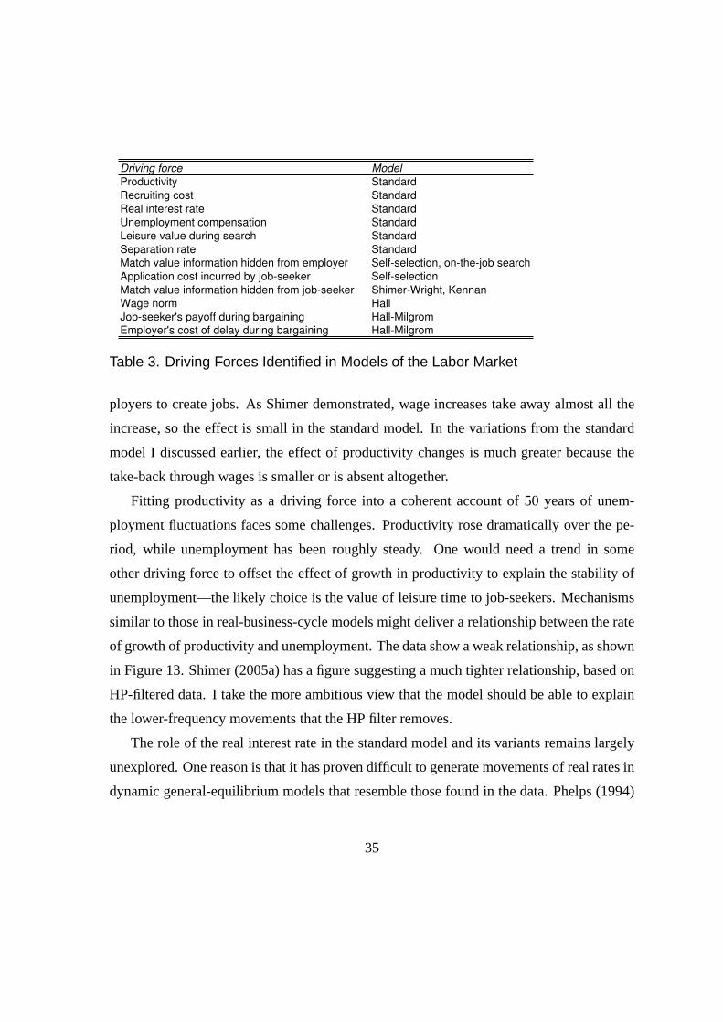
Driving force Model

Productivity Standard

Recruiting cost Standard

Real interest rate Standard

Unemployment compensation Standard

Leisure value during search Standard

Separation rate Standard

Match value information hidden from employer Self-selection, on-the-job search

Application cost incurred by job-seeker Self-selection

Match value information hidden from job-seeker Shimer-Wright, Kennan

Wage norm Hall

Job-seeker's payoff during bargaining Hall-Milgrom

Employer's cost of delay during bargaining Hall-Milgrom

Table 3. Driving Forces Identified in Models of the Labor Market

ployers to create jobs. As Shimer demonstrated, wage increases take away almost all the

increase, so the effect is small in the standard model. In the variations from the standard

model I discussed earlier, the effect of productivity changes is much greater because the

take-back through wages is smaller or is absent altogether.

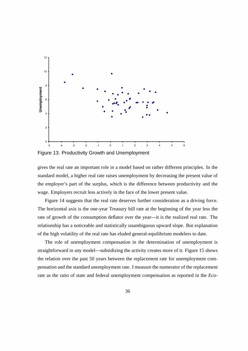
Fitting productivity as a driving force into a coherent account of 50 years of unem-

ployment fluctuations faces some challenges. Productivity rose dramatically over the pe-

riod, while unemployment has been roughly steady. One would need a trend in some

other driving force to offset the effect of growth in productivity to explain the stability of

unemployment—the likely choice is the value of leisure time to job-seekers. Mechanisms

similar to those in real-business-cycle models might deliver a relationship between the rate

of growth of productivity and unemployment. The data show a weak relationship, as shown

in Figure 13. Shimer (2005a) has a figure suggesting a much tighter relationship, based on

HP-filtered data. I take the more ambitious view that the model should be able to explain

the lower-frequency movements that the HP filter removes.

The role of the real interest rate in the standard model and its variants remains largely

unexplored. One reason is that it has proven difficult to generate movements of real rates in

dynamic general-equilibrium models that resemble those found in the data. Phelps (1994)

35

0

2

4

6

8

10

12

-5 -4 -3 -2 -1 0 1 2 3 4 5 6

Lagged Productivity Growth

Un

em

plo

ym

en

t

Figure 13. Productivity Growth and Unemployment

gives the real rate an important role in a model based on rather different principles. In the

standard model, a higher real rate raises unemployment by decreasing the present value of

the employer’s part of the surplus, which is the difference between productivity and the

wage. Employers recruit less actively in the face of the lower present value.

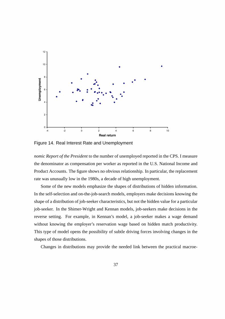
Figure 14 suggests that the real rate deserves further consideration as a driving force.

The horizontal axis is the one-year Treasury bill rate at the beginning of the year less the

rate of growth of the consumption deflator over the year—it is the realized real rate. The

relationship has a noticeable and statistically unambiguous upward slope. But explanation

of the high volatility of the real rate has eluded general-equilibrium modelers to date.

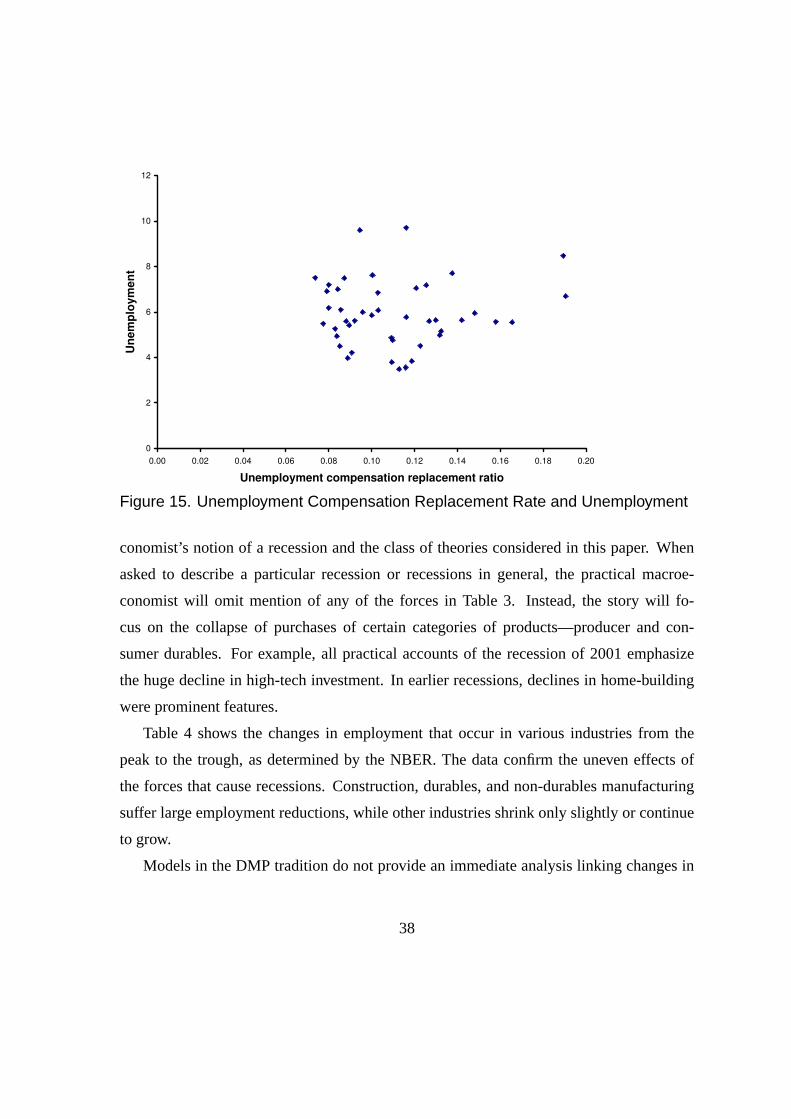
The role of unemployment compensation in the determination of unemployment is

straightforward in any model—subsidizing the activity creates more of it. Figure 15 shows

the relation over the past 50 years between the replacement rate for unemployment com-

pensation and the standard unemployment rate. I measure the numerator of the replacement

rate as the ratio of state and federal unemployment compensation as reported in theEco-

36

0

2

4

6

8

10

12

-4 -2 0 2 4 6 8 10

Real return

Un

em

plo

ym

en

t

Figure 14. Real Interest Rate and Unemployment

nomic Report of the Presidentto the number of unemployed reported in the CPS. I measure

the denominator as compensation per worker as reported in the U.S. National Income and

Product Accounts. The figure shows no obvious relationship. In particular, the replacement

rate was unusually low in the 1980s, a decade of high unemployment.

Some of the new models emphasize the shapes of distributions of hidden information.

In the self-selection and on-the-job-search models, employers make decisions knowing the

shape of a distribution of job-seeker characteristics, but not the hidden value for a particular

job-seeker. In the Shimer-Wright and Kennan models, job-seekers make decisions in the

reverse setting. For example, in Kennan’s model, a job-seeker makes a wage demand

without knowing the employer’s reservation wage based on hidden match productivity.

This type of model opens the possibility of subtle driving forces involving changes in the

shapes of those distributions.

Changes in distributions may provide the needed link between the practical macroe-

37

0

2

4

6

8

10

12

0.00 0.02 0.04 0.06 0.08 0.10 0.12 0.14 0.16 0.18 0.20

Unemployment compensation replacement ratio

Un

em

plo

ym

en

t

Figure 15. Unemployment Compensation Replacement Rate and Unemployment

conomist’s notion of a recession and the class of theories considered in this paper. When

asked to describe a particular recession or recessions in general, the practical macroe-

conomist will omit mention of any of the forces in Table 3. Instead, the story will fo-

cus on the collapse of purchases of certain categories of products—producer and con-

sumer durables. For example, all practical accounts of the recession of 2001 emphasize

the huge decline in high-tech investment. In earlier recessions, declines in home-building

were prominent features.

Table 4 shows the changes in employment that occur in various industries from the

peak to the trough, as determined by the NBER. The data confirm the uneven effects of

the forces that cause recessions. Construction, durables, and non-durables manufacturing

suffer large employment reductions, while other industries shrink only slightly or continue

to grow.

Models in the DMP tradition do not provide an immediate analysis linking changes in

38

Industry

Emloyment

change during

recessions

Construction -5.5

Durables -11.4

Nondurables -4.2

Wholesale -0.9

Retail -1.0

Finance 1.4

Prof. and bus. services -0.9

Ed. and health services 2.1

Leisure and hospitality -0.3

Other services 1.7

Government 1.4

Table 4. Peak-to-Trough Employment Changes by Industry, Averages over Reces-sions, 1948-2001

39

the industry composition of employment to the aggregate unemployment rate. As Section

2 of this paper documented, the flows of separations corresponding to the employment

changes in Table 4 are insignificant in comparison to the normal flows of separations. The

rise in unemployment is the result of diminished job-creation among employers in general.

The new additions to the DMP class of models may offer some hope of linking the

facts in Table 4 to the dramatic rise in unemployment that accompanies every recession.

For example, the events leading to a large decline in employment in durables might shift

the economy from the favorable equilibrium described in the self-selection model to the

unfavorable one. In the favorable equilibrium, the applicants for a job opening are largely

people who know they are qualified. Employers waste few resources screening out unsuit-

able applicants. They are correspondingly enthusiastic about creating jobs, so the market

is tight. A subtle change in the distribution of the signal that workers receive about their

likelihood of qualification can move the equilibrium perversely. Applicants, finding it dif-

ficult to locate any job, apply for jobs where they are less likely to be qualified. Employers

are overwhelmed by applicants and dissipate resources screening out the unqualified ones.

The market becomes slack, with high unemployment.

In Kennan’s model, the shape of the distribution of match productivity, a variable ob-

served only by the employer, has two key roles. Job-seekers know the distribution but not

the realization, so they solve a wage-bidding problem defined by the distribution. Firms

earn an informational rent on the difference between the productivity realization and the

wage bid. Shifts in the distribution induced by changes in the composition of employment

might result in changes in the rent.

Shimer and Wright’s model also has a distribution of individual productivity where the

realization is hidden from the worker. Changes in the shape of this distribution may have

important effects on the equilibrium job-finding rate in the model.

The successful model of fluctuations in the job-finding rate will incorporate on-the-job

search, as emphasized by Nagypal and Krause-Lubik.

40

8 Concluding Remarks

The job-finding rate is the key variable in understanding the large fluctuations in unemploy-

ment over the past 50 years. The separation rate, the other determinant of unemployment,

has been stable, by all the available evidence. Movements of the job-finding rate occur at

cyclical frequencies—the rate plunges in every recession. Movements also occur at low

frequency—the rate remained low even at the peaks in the 1950s and early 1960s and again

in the 1970s through the end of the 1980s.

Research has not yet settled on the exogenous driving forces that cause the secular

and cyclical movements of the job-finding rate. Productivity and the real interest rate are

modestly correlated with unemployment. New theories have added to the list of driving

forces, including some that raise interesting measurement challenges.

Recent thinking has added many amplification mechanisms that help explain the strong

response of unemployment to what appear to be small changes in exogenous driving forces.

Wage stickiness is moderately plausible as an explanation of the movements of the job-

finding rate over periods of a year or two. The substantial swings of labor-market conditions

over longer periods seem beyond this explanation. More subtle changes in the economic

environment seem promising ways to explain the movements of the job-finding rate at both

cyclical and subcyclical frequencies.

The business cycle appears to be a complicated phenomenon. I am convinced that

the labor market is the place to look for an understanding of the depth and persistence

of recessions. The turnover view is surely helpful in understanding these issues. The

explosion of recent research on amplification mechanisms seems to be leading in a direction

that will create a rich theory capable of explaining the volatility and amplitude of cyclical

and other fluctuations in the job-finding rate.

41

References

Barro, Robert J., “Long-Term Contracting, Sticky Prices, and Monetary Policy,”Journal

of Monetary Economics, July 1977,3 (3), pp. 305–316.

Binmore, Ken, Ariel Rubinstein, and Asher Wolinsky, “The Nash Bargaining Solution

in Economic Modeling,”RAND Journal of Economics, Summer 1986,17 (2), pp.

176–188.

Burdett, Kenneth and Dale T. Mortensen, “Wage Differentials, Employer Size,and Unem-

ployment,”International Economic Review, 1998,39 (2), pp. 257–273.

Davis, Steven and John Haltiwanger, “Gross Job Creation, Gross Job Destruction, and

Employment Reallocation,”Quarterly Journal of Economics, August 1992,107 (3),

819–863.

Diamond, Peter A., “Aggregate Demand Management in Search Equilibrium,”Journal of

Political Economy, October 1982,90 (5), pp. 881–894.

Gertler, Mark and Antonella Trigari, “Unemployment Fluctuations with Staggered Nash

Wage Bargaining,” May 2005. NYU Department of Economics.

Gottschalk, Peter and Robert A. Moffitt, “Job Instability and Insecurity for Males and

Females in the 1980s and 1990s.” In Neumark, ed (2000) pp. 142–195.

Hagedorn, Marcus and Iourii Manovskii, “The Cyclical Behavior of Equilibrium Unem-

ployment and Vacancies Revisited,” April 2005. University of Frankfurt.

Hall, Robert E., “Lost Jobs,”Brookings Papers on Economic Activity, 1995,1995(1), pp.

221–273.

, “The Amplification of Unemployment Fluctuations through Self-Selection,” 2005.

NBER Working Paper 11186.

42

, “Employment Fluctuations with Equilibrium Wage Stickiness,”American Economic

Review, March 2005,95 (1), 50–65.

and Paul R. Milgrom, “The Limited Influence of Unemployment on the Wage Bar-

gain,” February 2005. NBER Working Paper 11245.

Harris, John R. and Michael P. Todaro, “Migration, Unemployment and Development: A

Two-Sector Analysis,”American Economic Review, March 1970,60 (1), 126–42.

Jaeger, David A. and Ann Huff Stevens, “Is Job Stability in the United States Falling?

Reconciling Trends in the Current Population Survey and the Panel Study of Income

Dynamics.” In Neumark, ed (2000) pp. 31–69.

Kennan, John, “Private Information, Wage Bargaining, and Employment Fluctuations,”

May 2005. Department of Economics, University of Wisconsin.

Kodrzycki, Yolanda K., “Discouraged and Other Marginally Attached Workers: Evidence

on Their Role in the Labor Market,”New England Economic Review, May/June 2000,

pp. 35–40.

Krause, Michael U. and Thomas A. Lubik, “On-the-Job Search and the Cyclical Dynamics

of the Labor Market,” September 2004. Departments of Economics, Tilburg Univer-

sity and John Hopkins University.

Mortensen, Dale T., “Property Rights and Efficiency in Mating, Racing, and Related

Games,”American Economic Review, 1982,72 (5), pp. 968–979.

, “More on Unemployment and Vacancy Fluctuations,” June 2005. Department of

Economics, Northwestern University.

Nagypal, Eva, “Worker Reallocation over the Business Cycle: The Importance of Job-to-

Job Transitions, Part 1: Evidence,” July 2004. Department of Economics, Northwest-

ern University.

43

, “Worker Reallocation over the Business Cycle: The Importance of Job-to-Job Tran-

sitions, Part 2: Theory,” August 2004. Department of Economics, Northwestern Uni-

versity.

Neumark, David, ed.,On the Job: Is Long-Term Employment a Thing of the Past?, New

York: Russell Sage Foundation, 2000.

Phelps, Edmund,Structural Slumps, Cambridge: Harvard University Press, 1994.

Pissarides, Christopher, “Short-Run Equilibrium Dynamics of Unemployment, Vacancies,

and Real Wages,”American Economic Review, 1985,75 (4), pp. 676–690.

Shimer, Robert, “The Consequences of Rigid Wages in Search Models,”Journal of the

European Economic Association (Papers and Proceedings), 2004,2, 469–479.

, “The Cyclical Behavior of Equilibrium Unemployment and Vacancies,”American

Economic Review, March 2005,95 (1), 25–49.

, “The Cyclicality of Hires, Separations, and Job-to-Job Transitions,” January 30

2005. Department of Economics, University of Chicago.

, “Reassessing the Ins and Outs of Unemployment,” June 2005. Department of Eco-

nomics, University of Chicago.

and Randall Wright, “Competitive Search Equilibrium with Asymmetric Informa-

tion,” August 2004. Departments of Economics, University of Chicago and University

of Pennsylvania.

Tawara, Norikazu, “Search and Matching with Wage Bargaining under Asymmetric Infor-

mation,” March 2005. Departments of Economics, University of Chicago.

44