United States Office of Research and EPA/600/R-98/091 Environmental Protection Development August 1998 Agency Washington DC 20460

Environmental Technology Verification Report

Soil Sampling Technology

Clements Associates, Inc.JMC Environmentalist’s Subsoil Probe

Environmental Technology Verification Report

Soil Sampler

Clements Associates, Inc.

EP N600/R -98/091 August1998

JMC Environmentalist's Subsoil Probe

Prepared by

Tetra Tech EM Inc. 591 Camino De La Reina, Suite 640

San Diego, California 92108

Contract No. 68-CS-0037

Dr. Stephen Billets Characterization and Monitoring Branch

Environmental Sciences Division Las Vegas, Nevada 89193-3478

National Exposure Research Laboratory Office of Research and Development

U.S. Environmental Protection

ET~

Notice

This document was prepared for the U.S. Environmental Protection Agency’s (EPA) Superfund Innovative Technology Evaluation Program under Contract No. 68-C5-0037. The work detailed in this document was administered by the National Exposure Research Laboratory—Environmental Sciences Division in Las Vegas, Nevada. The document has been subjected to EPA’s peer and administrative reviews, and has been approved for publication as an EPA document. Mention of corporation names, trade names, or commercial products does not constitute endorsement or recommendation for use of specific products.

ii

UNITED STATES ENVIRONMENTAL PROTECTION AGENCY Office of Research and Development

Washington, D.C. 20460

Er/ ENVIRONMENTAL TECHNOLOGY VERIFICATION PROGRAM

VERIFICATION STATEMENT

TECHNOLOGY TYPE: SOIL SAMPLER

APPLICATION: SUBSURFACE SOIL SAMPLING

TECHNOLOGY NAME: JMC ENVIRONMENTALIST'S SUBSOIL PROBE

COMPANY: ADDRESS:

PHONE:

CLEMENTS ASSOCIATES, INC. 1992 HUNTER A VENUE NEWTON, lOW A 50208

(515) 792-8285

ETV PROGRAM DESCRIPTION

•••• •.to :-.·~.·· ............ ~-···· •••••••••• ••••• •••• .. ......................... ·.······:·· ••

.I ~~

I !

=·

The U.S. Environmental Protection Agency (EPA) created the Environmental Technology Verification (ETV) Program to facilitate the deployment of innovative technologies through performance verification and information dissemination. The goal of the ETV Program is to further environmental protection by substantially accelerating the acceptance and use of improved and cost-effective technologies. The ETV Program is intended to assist and inform those involved in the design, distribution, permitting, and purchase of environmental technologies. This document summarizes results of a demonstration of the Clements Associates, Inc. JMC Environmentalist's Subsoil Probe (ESP).

PROGRAM OPERATION

Under the ETV Program and with the full participation of the technology developer, the EPA evaluates the performance of innovative technologies by developing demonstration plans, conducting field tests, collecting and analyzing demonstration data, and preparing reports. The technologies are evaluated under rigorous quality assurance (QA) protocols to ensure that data of known and adequate quality are generated and that the demonstration results are defensible. The EPA's National Exposure Research Laboratory, which demonstrates field characterization and monitoring technologies, selected Tetra Tech EM Inc. as the verification organization to assist in field testing various soil and soil gas sampling technologies. This demonstration was conducted under the EPA's Superfund Innovative Technology Evaluation Program.

DEMONSTRATION DESCRIPTION

In May and June 1997, the EPA conducted a field test of the ESP along with three other soil and two soil gas sampling technologies. This verification statement focuses on the ESP; similar statements have been prepared for each of the other technologies. The performance of the ESP was compared to a reference subsurface soil sampling method (hollow-stem auger drilling and split-spoon sampling) in terms of the following parameters: (1) sample recovery, (2) volatile organic compound (VOC) concentrations in recovered samples, (3) sample integrity, (4) reliability and throughput, and (5) cost. Data quality indicators for precision, accuracy, representativeness, completeness, and comparability were also assessed against project-specific QA objectives to ensure the usefulness of the data.

The ESP was demonstrated at two sites: the Small Business Administration (SBA) site in Albert City, Iowa, and the Chemical Sales Company (CSC) site in Denver, Colorado. These sites were chosen because of the wide range ofVOC concentrations detected at the sites and because each has a distinct soil type. The VOCs detected at the sites include

EPA-VS-SCM-23 The accompanying notice is an integral part of this verification statement August 1998

iii

cis-1,2-dichloroethene (cis-1,2-DCE); 1,1,1-trichloroethane (1,1,1-TCA); trichloroethene (TCE); and tetrachloroethene (PCE). The SBA site is composed primarily of clay soil, and the CSC site is composed primarily of medium- to fine-grained sandy soil. A complete description of the demonstration, including a data summary and discussion of results, is available in the report titled Environmental Technology Verification Report: Soil Sampler, Clements Associates, Inc., JMC Environmentalist’s Subsoil Probe, EPA/600/R-98/091.

TECHNOLOGY DESCRIPTION

The ESP sampler is designed to collect subsurface soil samples and may be advanced by using manual or powered percussive techniques. The ESP can collect continuous or discrete samples. The ESP consists of a sampling tube, a body that guides the sampler as it is driven, and a foot-pedal-operated jack that retrieves the sampler. The sampler is a 36-inch long, solid barrel, open tube with an outside diameter of 1.125 inches. The sample tube is fitted with an inner sample liner and one of three interchangeable tips: a solid drive point, a standard cutting tip, or a wet cutting tip. The sampler is constructed of heat-treated 4130 alloy steel with nickel plating; the cutting tips and drive point are stainless steel. Liners facilitate retrieval of the sample and may be used for storage when applicable. The liner used for the demonstration was a 36-inch long by 0.90-inch inside diameter, thin-walled clear plastic tube that fits inside the sampler. It is capable of recovering a sample 36 inches long in the form of a soil core. Stainless steel liners are also available to meet the sample collection requirements and data quality objectives of a specific project.

VERIFICATION OF PERFORMANCE

The demonstration data indicate the following performance characteristics for the ESP:

Sample Recovery: For the purposes of this demonstration, sample recovery was defined as the ratio of the length of recovered sample to the length of sampler advancement. Sample recoveries from 28 samples collected at the SBA site ranged from 42 to 100 percent, with an average sample recovery of 96 percent. Sample recoveries from 42 samples collected at the CSC site ranged from 72 to 100 percent, with an average sample recovery of 95 percent. Using the reference method, sample recoveries from 42 samples collected at the SBA site ranged from 40 to 100 percent, with an average recovery of 88 percent. Sample recoveries from the 41 samples collected at the CSC site ranged from 53 to 100 percent, with an average recovery of 87 percent. A comparison of recovery data from the ESP sampler and the reference sampler indicates that the ESP achieved higher sample recoveries in both the clay soil at the SBA site and in the sandy soil at the CSC site relative to the sample recoveries achieved by the reference sampling method.

Volatile Organic Compound Concentrations: Soil samples collected using the ESP and the reference sampling method at five sampling depths in eight grids (four at the SBA site and four at the CSC site) were analyzed for VOCs. For 16 of the 18 ESP and reference sampling method pairs (seven at the SBA site and 11 at the CSC site), a statistical analysis using the Mann-Whitney test indicated no significant statistical difference at the 95 percent level between VOC concentrations in samples collected with the ESP and those collected with the reference sampling method. A statistically significant difference was identified for one sample pair collected at the SBA site and one sample pair at the CSC site. Analysis of the CSC site data, using the sign test, indicated no statistical difference between the data obtained by the ESP and the reference sampling method. However, at the SBA site, the sign test indicated that the data obtained by the ESP are statistically significantly different than the data obtained by the reference sampling method, suggesting that the reference method tends to yield higher concentrations in sampling fine-grained soils than does the ESP.

Sample Integrity: Seven integrity samples were collected with each sampling method at the SBA site, and five integrity samples were collected with each sampling method at the CSC site to determine if potting soil in a lined sampler became contaminated after it was advanced through a zone of high VOC concentrations. For the ESP, VOCs were detected in two of the 12 integrity samples: both at the SBA site. One of the integrity samples collected at the SBA site contained cis-1,2-DCE at 5,700 micrograms per kilogram (Fg/kg), TCE at 4,070 Fg/kg, and PCE at 212 Fg/kg; the other sample contained cis-1,2-DCE at 114 Fg/kg and TCE at 3.17 Fg/kg. These results indicate that the integrity of a lined chamber of the ESP may not be preserved when the sampler is advanced through highly contaminated soils. Results of sample integrity tests for the reference sampling method indicated no contamination in the potting soil after it was advanced through a zone of high VOC concentrations. Because potting soil has an

EPA-VS-SCM-23 The accompanying notice is an integral part of this verification statement August 1998

iv

organic carbon content many times greater than typical soils, the integrity tests represent a worst-case scenario for VOC absorbance and may not be representative of cross-contamination under normal field conditions.

Reliability and Throughput: At both the SBA and CSC sites, the ESP collected a sample from the desired depth on the initial attempt 100 percent of the time. Two target zones were not sampled at the SBA site due to the technology developer’s absence on several days during the demonstration; however, no planned samples were omitted due to equipment failure. Collection of saturated soil samples using the ESP at 40 feet below ground surface (bgs) in Grid 5 at the CSC site was not attempted because the sample depth was beyond the ESP’s performance range. For the reference sampling method, the initial sampling success rates at the SBA and CSC sites were 90 and 95 percent, respectively. Success rates for the reference sampling method were less than 100 percent due to (1) drilling beyond the target sampling depth, (2) insufficient sample recovery, or (3) auger refusal. The average sample retrieval time for a single operator to set up the ESP on a sampling point, collect the specified sample, backfill the hole with granular bentonite, decontaminate the sampler, and move to a new sampling location at the SBA site was 36.9 minutes per sample. The average sample retrieval time at the SBA site was 22.5 minutes per sample when two operators were used. Two operators were used for all grids sampled at the CSC site, resulting in an average sample retrieval time of 13.4 minutes per sample. For the reference sampling method, the average sample retrieval times at the SBA and CSC sites were 26 and 8.4 minutes per sample, respectively. A three-person sampling crew collected soil samples using the reference sampling method at both sites. One additional person was present at the CSC site to oversee and assist with sample collection using the reference method.

Cost: Based on the demonstration results and information provided by the vendor, the ESP can be purchased for $2,780 or rented for $250 per day. The optional electric hammer and generator can be rented for $150 to $300 per day. Operating costs for the ESP ranged from $2,480 to $4,210 at the clay soil site and $1,880 to $3,110 at the sandy soil site. For this demonstration, the reference sampling was procured at a lump sum rate of $13,700 for the clay soil site and $7,700 for the sandy soil site. Oversight costs for the reference method ranged from $4,230 to $6,510 at the clay soil site and $1,230 to $2,060 at the sandy soil site. A site-specific cost and performance analysis is recommended before selecting a soil sampling method.

A qualitative performance assessment of the ESP indicated that (1) the sampler is easy to use and requires no specialized training to operate; (2) logistical requirements are generally less than those of the reference sampling method; (3) sample handling is similar to the reference method; (4) the performance range is limited by the advancement platform, although the ESP successfully retrieved a sample on one of two sampling attempts at depths greater than 25 feet; and (5) no drill cuttings are generated when using the ESP.

The demonstration results indicate that the ESP can provide useful, cost-effective samples for environmental problem­solving. However, in some cases, VOC data collected using the ESP may be statistically different from VOC data collected using the reference sampling method. Also, the integrity of a lined sample chamber may not be preserved when the sampler is advanced through highly contaminated clay soils. As with any technology selection, the user must determine what is appropriate for the application and project data quality objectives.

Gary J. Foley, Ph.D. Director National Exposure Research Laboratory Office of Research and Development

NOTICE: EPA verifications are based on an evaluation of technology performance under specific, predetermined criteria and appropriate quality assurance procedures. EPA makes no expressed or implied warranties as to the performance of the technology and does not certify that a technology will always operate as verified. The end user is solely responsible for complying with any and all applicable federal, state, and local requirements.

EPA-VS-SCM-23 The accompanying notice is an integral part of this verification statement August 1998

v

Foreword

The U.S. Environmental Protection Agency (EPA) is charged by Congress with protecting the nation’s natural resources. Under the mandate of national environmental laws, the Agency strives to formulate and implement actions leading to a compatible balance between human activities and the ability of natural systems to support and nurture life. To meet this mandate, the EPA’s Office of Research and Development (ORD) provides data and science support that can be used to solve environmental problems and to build the scientific knowledge base needed to manage our ecological resources wisely, to understand how pollutants affect our health, and to prevent or reduce environmental risks.

The National Exposure Research Laboratory (NERL) is the Agency’s center for the investigation of technical and management approaches for identifying and quantifying risks to human health and the environment. Goals of the Laboratory’s research program are to (1) develop and evaluate technologies for characterizing and monitoring air, soil, and water; (2) support regulatory and policy decisions; and (3) provide the science support needed to ensure effective implementation of environmental regulations and strategies.

The EPA’s Superfund Innovative Technology Evaluation (SITE) Program evaluates technologies for the characterization and remediation of contaminated Superfund and Resource Conservation and Recovery Act sites. The SITE Program was created to provide reliable cost and performance data to speed the acceptance and use of innovative remediation, characterization, and monitoring technologies by the regulatory and user community.

Effective measurement and monitoring technologies are needed to assess the degree of contamination at a site, to provide data that can be used to determine the risk to public health or the environment, to supply the necessary cost and performance data to select the most appropriate technology, and to monitor the success or failure of a remediation process. One component of the EPA SITE Program, the Monitoring and Measurement Technology Program, demonstrates and evaluates innovative technologies to meet these needs.

Candidate technologies can originate from within the federal government or from the private sector. Through the SITE Program, developers are given the opportunity to conduct a rigorous demonstration of their technology under actual field conditions. By completing the evaluation and distributing the results, the Agency establishes a baseline for acceptance and use of these technologies. The Monitoring and Measurement Technology Program is managed by the ORD’s Environmental Sciences Division in Las Vegas, Nevada.

Gary Foley, Ph.D. Director National Exposure Research Laboratory Office of Research and Development

vi

Contents

Notice . . . . . . . . . . . . . . . . . . . . . . . . . . . . . . . . . . . . . . . . . . . . . . . . . . . . . . . . . . . iiVerification Statement . . . . . . . . . . . . . . . . . . . . . . . . . . . . . . . . . . . . . . . . . . . . . . . . iiiForeword . . . . . . . . . . . . . . . . . . . . . . . . . . . . . . . . . . . . . . . . . . . . . . . . . . . . . . . . viFigures . . . . . . . . . . . . . . . . . . . . . . . . . . . . . . . . . . . . . . . . . . . . . . . . . . . . . . . . . ixTables . . . . . . . . . . . . . . . . . . . . . . . . . . . . . . . . . . . . . . . . . . . . . . . . . . . . . . . . . . . xAcronyms and Abbreviations . . . . . . . . . . . . . . . . . . . . . . . . . . . . . . . . . . . . . . . . . . . xiAcknowledgments . . . . . . . . . . . . . . . . . . . . . . . . . . . . . . . . . . . . . . . . . . . . . . . . . . xiiExecutive Summary . . . . . . . . . . . . . . . . . . . . . . . . . . . . . . . . . . . . . . . . . . . . . . . . . xiii

Chapter 1 Introduction . . . . . . . . . . . . . . . . . . . . . . . . . . . . . . . . . . . . . . . . . . . . . . . . 1Technology Verification Process . . . . . . . . . . . . . . . . . . . . . . . . . . . . . . . . 3

Needs Identification and Technology Selection . . . . . . . . . . . . . . . . . . . . . 3Demonstration Planning and Implementation . . . . . . . . . . . . . . . . . . . . . . 3Report Preparation . . . . . . . . . . . . . . . . . . . . . . . . . . . . . . . . . . . . . . . 4Information Distribution . . . . . . . . . . . . . . . . . . . . . . . . . . . . . . . . . . . 4

Demonstration Purpose . . . . . . . . . . . . . . . . . . . . . . . . . . . . . . . . . . . . . . 4

Chapter 2 Technology Description . . . . . . . . . . . . . . . . . . . . . . . . . . . . . . . . . . . . . . . . 5Background . . . . . . . . . . . . . . . . . . . . . . . . . . . . . . . . . . . . . . . . . . . . . 5Components and Accessories . . . . . . . . . . . . . . . . . . . . . . . . . . . . . . . . . . . 5Description of Platforms . . . . . . . . . . . . . . . . . . . . . . . . . . . . . . . . . . . . . 7General Operating Procedures . . . . . . . . . . . . . . . . . . . . . . . . . . . . . . . . . . 7Developer Contact . . . . . . . . . . . . . . . . . . . . . . . . . . . . . . . . . . . . . . . . 13

Chapter 3 Site Descriptions and Demonstration Design . . . . . . . . . . . . . . . . . . . . . . . . . . . 14Site Selection and Description . . . . . . . . . . . . . . . . . . . . . . . . . . . . . . . . . 14

SBA Site Description . . . . . . . . . . . . . . . . . . . . . . . . . . . . . . . . . . . . 14CSC Site Description . . . . . . . . . . . . . . . . . . . . . . . . . . . . . . . . . . . . 16

Predemonstration Sampling and Analysis . . . . . . . . . . . . . . . . . . . . . . . . . . 18Demonstration Design . . . . . . . . . . . . . . . . . . . . . . . . . . . . . . . . . . . . . . 19

Sample Recovery . . . . . . . . . . . . . . . . . . . . . . . . . . . . . . . . . . . . . . . 20Volatile Organic Compound Concentrations . . . . . . . . . . . . . . . . . . . . . . 20Sample Integrity . . . . . . . . . . . . . . . . . . . . . . . . . . . . . . . . . . . . . . . 25Reliability and Throughput . . . . . . . . . . . . . . . . . . . . . . . . . . . . . . . . 25Cost . . . . . . . . . . . . . . . . . . . . . . . . . . . . . . . . . . . . . . . . . . . . . . . 26Deviations from the Demonstration Plan . . . . . . . . . . . . . . . . . . . . . . . . 26

Chapter 4 Description and Performance of the Reference Method . . . . . . . . . . . . . . . . . . . . 27Background . . . . . . . . . . . . . . . . . . . . . . . . . . . . . . . . . . . . . . . . . . . . 27Components and Accessories . . . . . . . . . . . . . . . . . . . . . . . . . . . . . . . . . . 27Description of Platform . . . . . . . . . . . . . . . . . . . . . . . . . . . . . . . . . . . . . 27Demonstration Operating Procedures . . . . . . . . . . . . . . . . . . . . . . . . . . . . . 29Qualitative Performance Factors . . . . . . . . . . . . . . . . . . . . . . . . . . . . . . . . 31

Reliability and Ruggedness . . . . . . . . . . . . . . . . . . . . . . . . . . . . . . . . 31Training Requirements and Ease of Operation . . . . . . . . . . . . . . . . . . . . 32

vii

Contents (Continued)

Logistical Requirements . . . . . . . . . . . . . . . . . . . . . . . . . . . . . . . . . . 32Sample Handling . . . . . . . . . . . . . . . . . . . . . . . . . . . . . . . . . . . . . . . 32Performance Range . . . . . . . . . . . . . . . . . . . . . . . . . . . . . . . . . . . . . 32Investigation-Derived Waste . . . . . . . . . . . . . . . . . . . . . . . . . . . . . . . . 33

Quantitative Performance Factors . . . . . . . . . . . . . . . . . . . . . . . . . . . . . . . 33Sample Recovery . . . . . . . . . . . . . . . . . . . . . . . . . . . . . . . . . . . . . . . 33Volatile Organic Compound Concentrations . . . . . . . . . . . . . . . . . . . . . . 33Sample Integrity . . . . . . . . . . . . . . . . . . . . . . . . . . . . . . . . . . . . . . . 35Sample Throughput . . . . . . . . . . . . . . . . . . . . . . . . . . . . . . . . . . . . . 35

Data Quality . . . . . . . . . . . . . . . . . . . . . . . . . . . . . . . . . . . . . . . . . . . . 35

Chapter 5 Technology Performance . . . . . . . . . . . . . . . . . . . . . . . . . . . . . . . . . . . . . . . 37Qualitative Performance Factors . . . . . . . . . . . . . . . . . . . . . . . . . . . . . . . . 37

Reliability and Ruggedness . . . . . . . . . . . . . . . . . . . . . . . . . . . . . . . . 37Training Requirements and Ease of Operation . . . . . . . . . . . . . . . . . . . . 38Logistical Requirements . . . . . . . . . . . . . . . . . . . . . . . . . . . . . . . . . . 38Sample Handling . . . . . . . . . . . . . . . . . . . . . . . . . . . . . . . . . . . . . . . 38Performance Range . . . . . . . . . . . . . . . . . . . . . . . . . . . . . . . . . . . . . 39Investigation-Derived Waste . . . . . . . . . . . . . . . . . . . . . . . . . . . . . . . . 39

Quantitative Performance Assessment . . . . . . . . . . . . . . . . . . . . . . . . . . . . 39Sample Recovery . . . . . . . . . . . . . . . . . . . . . . . . . . . . . . . . . . . . . . . 40Volatile Organic Compound Concentrations . . . . . . . . . . . . . . . . . . . . . . 40Sample Integrity . . . . . . . . . . . . . . . . . . . . . . . . . . . . . . . . . . . . . . . 46Sample Throughput . . . . . . . . . . . . . . . . . . . . . . . . . . . . . . . . . . . . . 47

Data Quality . . . . . . . . . . . . . . . . . . . . . . . . . . . . . . . . . . . . . . . . . . . . 47

Chapter 6 Economic Analysis . . . . . . . . . . . . . . . . . . . . . . . . . . . . . . . . . . . . . . . . . . 48Assumptions . . . . . . . . . . . . . . . . . . . . . . . . . . . . . . . . . . . . . . . . . . . . 48JMC Environmentalist’s Subsoil Probe . . . . . . . . . . . . . . . . . . . . . . . . . . . 48Reference Sampling Method . . . . . . . . . . . . . . . . . . . . . . . . . . . . . . . . . . 50

Chapter 7 Summary of Demonstration Results . . . . . . . . . . . . . . . . . . . . . . . . . . . . . . . . 53

Chapter 8 Technology Update . . . . . . . . . . . . . . . . . . . . . . . . . . . . . . . . . . . . . . . . . . 56

Chapter 9 Previous Deployment . . . . . . . . . . . . . . . . . . . . . . . . . . . . . . . . . . . . . . . . . 57

References . . . . . . . . . . . . . . . . . . . . . . . . . . . . . . . . . . . . . . . . . . . . . . . . . . . . . . . 58

Appendix

A Data Summary Tables and Statistical Method Descriptions . . . . . . . . . . . . . . . . . A-1

viii

Figures

2-1. JMC Environmentalist’s Subsoil Probe Components . . . . . . . . . . . . . . . . . . . . . . . . . 6

2-2. JMC Environmentalist’s Subsoil Probe Hammer Assembly and Extensions . . . . . . . . . . . 8

2-3. Operation of JMC Environmentalist’s Subsoil Probe: Sampler Loading and Advancement 10

2-4. Operation of JMC Environmentalist’s Subsoil Probe: Sample Retrieval . . . . . . . . . . . . 11

2-5. Operation of the JMC Environmentalist’s Subsoil Probe Footpedal . . . . . . . . . . . . . . . 12

3-1. Small Business Administration Site . . . . . . . . . . . . . . . . . . . . . . . . . . . . . . . . . . . 15

3-2. Chemical Sales Company Site . . . . . . . . . . . . . . . . . . . . . . . . . . . . . . . . . . . . . . 17

3-3. Typical Sampling Locations and Random Sampling Grid . . . . . . . . . . . . . . . . . . . . . 21

3-4. Sampling Grid with High Contaminant Concentration Variability . . . . . . . . . . . . . . . . 23

3-5. Sampling Grid with Low Contaminant Concentration Variability . . . . . . . . . . . . . . . . 24

4-1. Split-Spoon Soil Sampler . . . . . . . . . . . . . . . . . . . . . . . . . . . . . . . . . . . . . . . . . 28

4-2. Typical Components of a Hollow-Stem Auger . . . . . . . . . . . . . . . . . . . . . . . . . . . . 30

5-1. Comparative Plot of Median VOC Concentrations for the ESP and Reference Sampling Method at the SBA and CSC Sites . . . . . . . . . . . . . . . . . . . . . . . . . . . . . 45

ix

Tables

3-1. Sampling Depths Selected for the ESP Demonstration . . . . . . . . . . . . . . . . . . . . . . . 19

4-1. Volatile Organic Compound Concentrations in Samples Collected Using the Reference Sampling Method . . . . . . . . . . . . . . . . . . . . . . . . . . . . . . . . . . . . . . . . . . . . . . 34

5-1. Investigation-Derived Waste Generated During the Demonstration . . . . . . . . . . . . . . . 40

5-2. Sample Recoveries for the ESP and the Reference Sampling Method . . . . . . . . . . . . . . 40

5-3. Volatile Organic Compound Concentrations in Samples Collected Using the ESP . . . . . . 42

5-4. Demonstration Data Summary for the ESP and Reference Sampling Method . . . . . . . . . 43

5-5. Comparison of Median Volatile Organic Compound Concentrations of ESP andReference Sampler Data and Statistical Significance . . . . . . . . . . . . . . . . . . . . . . . . . 44

5-6. Sign Test Results for the ESP and the Reference Sampling Method . . . . . . . . . . . . . . . 46

5-7. Average Sample Retrieval Times for the ESP and the Reference Sampling Method . . . . . 47

6-1. Estimated Subsurface Soil Sampling Costs for the JMC Environmentalist’s Subsoil Probe . 49

6-2. Estimated Subsurface Soil Sampling Costs for the Reference Sampling Method . . . . . . . 51

x

Acronyms and Abbreviations

bgs below ground surface cc cubic centimeter cis-1,2-DCE cis-1,2-dichloroethene CME Central Mine Equipment CSC Chemical Sales Company 1,1-DCA 1,1-dichloroethane E&E Ecology & Environment EPA U.S. Environmental Protection Agency ESP Environmentalist’s Subsoil Probe ETV Environmental Technology Verification ETVR Environmental Technology Verification Report g gram GC gas chromatography IDW investigation-derived waste LCS laboratory control sample mg/kg milligrams per kilogram mL milliliter MS/MSD matrix spike/matrix spike duplicate Fg/kg micrograms per kilogram NERL National Exposure Research Laboratory OU operable unit PCE tetrachloroethene QA quality assurance QA/QC quality assurance/quality control RI/FS remedial investigation/feasibility study SOP standard operating procedures SBA Small Business Administration SITE Superfund Innovative Technology Evaluation SMC Superior Manufacturing Company 1,1,1-TCA 1,1,1-trichloroethane TCE trichloroethene VOC volatile organic compound

xi

Acknowledgments

This report was prepared for the U.S. Environmental Protection Agency’s (EPA) Environmental Technology Verification Program under the direction of Stephen Billets, Brian Schumacher, and Eric Koglin of the EPA’s National Exposure Research Laboratory—Environmental Sciences Division in Las Vegas, Nevada. The project was also supported by the EPA’s Superfund Innovative Technology Evaluation (SITE) Program. The EPA wishes to acknowledge the support of Janice Kroone (EPA Region 7), Joe Vranka (Colorado Department of Public Health and the Environment), Armando Saenz (EPA Region 8), Sam Goforth (independent consultant), Alan Hewitt (Cold Regions Research Engineering Laboratory), Bob Siegrist (Colorado School of Mines), and Ann Kern (EPA SITE Program). In addition, we gratefully acknowledge the collection of soil samples using the Environmentalist’s Subsoil Probe by Jim Clements (Clements Associates, Inc.), collection of soil samples using hollow-stem auger drilling and split-spoon sampling by Michael O’Malley, Bruce Stewart, and Clay Schnase (Geotechnical Services), implementation of this demonstration by Eric Hess, Patrick Splichal, and Scott Schulte (Tetra Tech); editorial and publication support by Butch Fries, Jennifer Brainerd, and Stephanie Anderson (Tetra Tech); and technical report preparation by Carl Rhodes, Ron Ohta, Roger Argus, and Ben Hough (Tetra Tech).

xii

Executive Summary

In May and June 1997, the U.S. Environmental Protection Agency (EPA) sponsored a demonstration of the Clements Associates, Inc. JMC Environmentalist’s Subsoil Probe (ESP), three other soil sampling technologies, and two soil gas sampling technologies. This Environmental Technology Verification Report presents the results of the ESP demonstration; similar reports have been published for each of the other soil and soil gas sampling technologies.

The ESP is a sampling tool capable of collecting unconsolidated subsurface material at depths that depend on the capability of the advancement platform. The ESP can be advanced into the subsurface with direct-push platforms, drill rigs, or manual methods.

The ESP was demonstrated at two sites: the Small Business Administration (SBA) site in Albert City, Iowa, and the Chemical Sales Company (CSC) site in Denver, Colorado. These sites were chosen because each has a wide range of volatile organic compound (VOC) concentrations and because each has a distinct soil type. The VOCs detected at the sites include cis-1,2-dichloroethene; trichloroethene; 1,1,1-trichloroethane; and tetrachloroethene. The SBA site is composed primarily of clay soil, and the CSC site is composed primarily of medium- to fine-grained sandy soil.

The ESP was compared to a reference subsurface soil sampling method (hollow-stem auger drilling and split-spoon sampling) in terms of the following parameters: (1) sample recovery, (2) VOC concentrations in recovered samples, (3) sample integrity, (4) reliability and throughput, and (5) cost. The demonstration data indicate the following performance and cost characteristics for the ESP:

C Compared to the reference method, average sample recoveries for the ESP were higher for both clay and sandy soils.

C A significant statistical difference between the VOC concentrations measured was detected for one of the seven ESP and reference sampling method pairs collected at the SBA site and for one of the 11 sampling pairs collected at the CSC site. The data also suggest that the reference sampling method tends to yield higher results than the ESP in sampling fine-grained soils.

C In two of the 12 integrity test samples, the integrity of a lined chamber of the ESP was not preserved when the sampler was advanced through highly contaminated clay soils.

C The reliability of the ESP to collect a sample in the first attempt was higher than that of the reference sampling method in both clay and sandy soils. The average sample retrieval time for the ESP using two operators was slightly quicker than the retrieval time for the reference method in clay soil but slower in sandy soil.

C For both clay soil and sandy soil sites, the range of costs for collecting soil samples using the ESP was lower than the reference sampling method. The actual cost depends on the number of samples required, the sample retrieval time, soil type, sample depth, and the cost for disposal of drill cuttings. A site-specific cost and performance analysis is recommended before selecting a subsurface soil sampling method.

In general, results for the data quality indicators selected for this demonstration met the established quality assurance objectives and support the usefulness of the demonstration results in verifying the Clements Associates, Inc. JMC ESP’s performance.

xiii

Chapter 1Introduction

Performance verification of innovative and alternative environmental technologies is an integral part of the U.S. Environmental Protection Agency’s (EPA) regulatory and research mission. Early efforts focused on evaluating technologies that supported implementation of the Clean Air and Clean Water Acts. To meet the needs of the hazardous waste program, the Superfund Innovative Technology Evaluation (SITE) Program was established by the EPA Office of Solid Waste and Emergency Response (OSWER) and Office of Research and Development (ORD) as part of the Superfund Amendments and Reauthorization Act of 1986. The primary purpose of the SITE Program is to promote the acceptance and use of innovative characterization, monitoring, and treatment technologies.

The overall goal of the SITE Program is to conduct research and performance verification studies of alternative or innovative technologies that may be used to achieve long-term protection of human health and the environment. The various components of the SITE Program are designed to encourage the development, demonstration, acceptance, and use of new or innovative treatment and monitoring technologies. The program is designed to meet four primary objectives: (1) identify and remove obstacles to the development and commercial use of alternative technologies, (2) support a development program that identifies and nurtures emerging technologies, (3) demonstrate promising innovative technologies to establish reliable performance and cost information for site characterization and cleanup decision-making, and (4) develop procedures and policies that encourage the selection of alternative technologies at Superfund sites, as well as other waste sites and commercial facilities.

The intent of a SITE demonstration is to obtain representative, high quality, performance and cost data on innovative technologies so that potential users can assess a given technology’s suitability for a specific application. The SITE Program includes the following elements:

C Monitoring and Measurement Technology (MMT) Program — Evaluates technologies that detect, monitor, sample, and measure hazardous and toxic substances. These technologies are expected to provide better, faster, and more cost-effective methods for producing real-time data during site characterization and remediation studies

C Remediation Technologies — Conducts demonstrations of innovative treatment technologies to provide reliable performance, cost, and applicability data for site cleanup

C Technology Transfer Program — Provides and disseminates technical information in the form of updates, brochures, and other publications that promote the program and the technology. Provides technical assistance, training, and workshops to support the technology

The MMT Program provides developers of innovative hazardous waste measurement, monitoring, and sampling technologies with an opportunity to demonstrate a technology’s performance under actual

1

field conditions. These technologies may be used to detect, monitor, sample, and measure hazardous and toxic substances in soil, sediment, waste materials, and groundwater. Technologies include chemical sensors for in situ (in place) measurements, groundwater sampling devices, soil and core sampling devices, soil gas samplers, laboratory and field-portable analytical equipment, and other systems that support field sampling or data acquisition and analysis.

The MMT Program promotes the acceptance of technologies that can be used to accurately assess the degree of contamination at a site, provide data to evaluate potential effects on human health and the environment, apply data to assist in selecting the most appropriate cleanup action, and monitor the effectiveness of a remediation process. Acceptance into the program places high priority on innovative technologies that provide more cost-effective, faster, and safer methods than conventional technologies for producing real-time or near-real-time data. These technologies are demonstrated under field conditions and results are compiled, evaluated, published, and disseminated by ORD. The primary objectives of the MMT Program are the following:

C Test field analytical technologies that enhance monitoring and site characterization capabilities

C Identify the performance attributes of new technologies to address field characterization and monitoring problems in a more cost-effective and efficient manner

C Prepare protocols, guidelines, methods, and other technical publications that enhance the acceptance of these technologies for routine use

The SITE MMT Program is administered by ORD’s National Exposure Research Laboratory (NERL-LV) at the Environmental Sciences Division in Las Vegas, Nevada.

In 1994, the EPA created the Environmental Technology Verification (ETV) Program to facilitate the deployment of innovative technologies in other areas of environmental concern through performance verification and information dissemination. As in the SITE Program, the goal of the ETV Program is to further environmental protection by substantially accelerating the acceptance and use of improved and cost-effective technologies. The ETV Program is intended to assist and inform those involved in the design, distribution, permitting, and purchase of various environmental technologies. The ETV Program capitalizes on and applies the lessons learned in implementing the SITE Program.

For each demonstration, the EPA draws on the expertise of partner "verification organizations" to design efficient procedures for conducting performance tests of environmental technologies. The EPA selects its partners from both the public and private sectors, including federal laboratories, states, universities, and private sector entities. Verification organizations oversee and report verification activities based on testing and quality assurance (QA) protocols developed with input from all major stakeholder and customer groups associated with the technology area. For this demonstration, the EPA selected Tetra Tech EM Inc. (Tetra Tech; formerly PRC Environmental Management, Inc.) as the verification organization.

In May and June 1997, the EPA conducted a demonstration, funded by the SITE Program, to verify the performance of four soil and two soil gas sampling technologies: SimulProbe® Technologies, Inc.,

® TMCore Barrel Sampler; Geoprobe Systems, Inc., Large-Bore Soil Sampler; AMS Dual Tube Liner Sampler; Clements Associates, Inc., Environmentalist’s Subsoil Probe; Quadrel Services, Inc., EMFLUX® Soil Gas Investigation System; and W.L. Gore & Associates GORE-SORBER® Soil Gas Sampler. This environmental technology verification report (ETVR) presents the results of the demonstration for one soil sampling technology, the JMC Environmentalist’s Subsoil Probe (ESP). Separate ETVRs have been published for the remaining soil and soil gas sampling technologies.

2

Technology Verification Process

The technology verification process is designed to conduct demonstrations that will generate high­quality data that the EPA and others can use to verify technology performance and cost. Four key steps are inherent in the process: (1) needs identification and technology selection, (2) demonstration planning and implementation, (3) report preparation, and (4) information distribution.

Needs Identification and Technology Selection

The first aspect of the technology verification process is to identify technology needs of the EPA and the regulated community. The EPA, the U.S. Department of Energy, the U.S. Department of Defense, industry, and state agencies are asked to identify technology needs for characterization, sampling, and monitoring. Once a technology area is chosen, a search is conducted to identify suitable technologies that will address that need. The technology search and identification process consists of reviewing responses to Commerce Business Daily announcements, searches of industry and trade publications, attendance at related conferences, and leads from technology developers. Selection of characterization and monitoring technologies for field testing includes an evaluation of the candidate technology against the following criteria:

C Designed for use in the field or in a mobile laboratory

C Applicable to a variety of environmentally contaminated sites

C Has potential for resolving problems for which current methods are unsatisfactory

C Has costs that are competitive with current methods

C Performs better than current methods in areas such as data quality, sample preparation, or analytical turnaround time

C Uses techniques that are easier and safer than current methods

C Is commercially available

Demonstration Planning and Implementation

After a technology has been selected, the EPA, the verification organization, and the developer agree to a strategy for conducting the demonstration and evaluating the technology. The following issues are addressed at this time:

C Identifying and defining the roles of demonstration participants, observers, and reviewers

C Identifying demonstration sites that provide the appropriate physical or chemical attributes in the desired environmental media

C Determining logistical and support requirements (for example, field equipment, power and water sources, mobile laboratory, or communications network)

C Arranging analytical and sampling support

3

C Preparing and implementing a demonstration plan that addresses the experimental design, the sampling design, quality assurance/quality control (QA/QC), health and safety, field and laboratory operations scheduling, data analysis procedures, and reporting requirements

Report Preparation

Each of the innovative technologies is evaluated independently and, when possible, against a reference technology. The technologies are usually operated in the field by the developers in the presence of independent observers. These individuals are selected by the EPA or the verification organization and work to ensure that the technology is operated in accordance with the demonstration plan. Demonstration data are used to evaluate the capabilities, performance, limitations, and field applications of each technology. After the demonstration, all raw and reduced data used to evaluate each technology are compiled into a technology evaluation report as a record of the demonstration. A verification statement and detailed evaluation narrative of each technology are published in an ETVR. This document receives a thorough technical and editorial review prior to publication.

Information Distribution

The goal of the information distribution strategy is to ensure that ETVRs are readily available to interested parties through traditional data distribution pathways, such as printed documents. Related documents and technology updates are also available on the World Wide Web through the ETV Web site (http://www.epa.gov/etv) and through the Hazardous Waste Clean-Up Information Web site supported by the EPA OSWER Technology Innovation Office (http://clu-in.org). Additional information on the SITE Program can be found on ORD’s web site (http://www.epa.gov/ORD/SITE).

Demonstration Purpose

The primary purpose of a soil sampling technology is to collect a sample from a specified depth and return it to the surface with minimal changes to the chemical concentration or physical properties of the sample. This report documents the performance of the ESP relative to the hollow-stem auger drilling and split-spoon sampling reference method.

This document summarizes the results of an evaluation of the ESP in comparison to the reference sampling method in terms of the following parameters: (1) sample recovery, (2) volatile organic compound (VOC) concentrations in recovered samples, (3) sample integrity, (4) reliability and throughput, and (5) cost. Data quality measures of precision, accuracy, representativeness, completeness, and comparability were also assessed against established QA objectives to ensure the usefulness of the data for the purpose of this verification.

4

Chapter 2Technology Description

This chapter describes the ESP, including its background, components and accessories, sampling platform, and general operating procedures. The text in this chapter was provided by the developer and was edited for format and relevance.

Background

The ESP was developed by Clements Associates, Inc., as a hand-operated soil sampler designed to collect discrete or continuous subsurface soil samples for chemical analysis. The ESP was designed for sampling to depths of 4 feet below ground surface (bgs); however, through the use of extensions, samples may be obtained from depths as great as 20 feet bgs in some soil types. The physical limitations on the operation of the ESP depend on the method of sampler advancement (manual or electric hammer) and the nature of the subsurface matrix. The technology is primarily restricted to unconsolidated soil free of large cobbles or boulders. Sediments containing gravel-sized material supported by a finer-grained matrix can also be sampled. Additional developer claims for the performance of the ESP are that it:

C Is simple to operate and requires no special training

C Is unaffected by variable field conditions

C Can be used to collect either discrete or continuous soil samples

C Can be used to characterize subsurface soil contamination

C Is easily transportable

However, during the demonstration only the developer’s claims regarding collection of representative discrete soil samples in the subsurface, operation of the ESP, and the ability of the ESP to be used to sample for VOCs were evaluated.

Components and Accessories

The major components of the ESP sampling system (Figure 2-1) are a sampling tube assembly, the ESP body, and a jack that is used to assist in sample retrieval. The primary component of the ESP sample tube assembly is a heat-treated 4130 alloy steel sample tube with nickel plating. The tube has a uniform 1.125-inch outer diameter and is 36 inches long. The sampling tube assembly also includes

5

HANDGRIP

ESP BODY

I

I el

"'S p

JACK LEVER

JACK

GROUND PAD

0

I ' I I I

I I It I I I I

1 I I I II

II I I I I I I I I

I: I I I I

I I I II

I I 1 I I

STOP RING

RUBBER BUMPER

HAMMER ASSEMBLY

THREADED COLLAR

t=~- IMPACT CUSHIONING WASHER

I ALUMINUM CYUNTR

Figure 2-1. JMC Environmentalist's Subsoil Probe Components (modified from Clements

Associates, Inc., 1997)

6

one of three interchangeable stainless steel tips (a solid drive point, standard cutting tip, or wet cutting tip) and an inner sample liner. Several types of sample liners are available; they include a 36-inch­long plastic liner and stainless steel liners. A 36-inch-long plastic liner with an inside diameter of 0.90 inch was used for this demonstration.

The ESP body serves as a base and guide for the sampling tube as it is driven into or retrieved from the borehole. The jack is used to retrieve the sampling tube. The jack also allows operators to smoothly lower the sampler and tool string into the hole at a controlled rate, minimizing disturbance to the borehole as the sampling tube is returned to the bottom of the hole for each new sample.

A 2-inch diameter, 6-inch long stainless steel concentric sampler tube is also available for use with the ESP. The concentric tube may be used to temporarily case off the uppermost 6 inches of soil, reducing the risk of cross-contaminating subsurface soil samples when using the ESP in areas with significant surface contamination. However, this accessory was not used during the demonstration.

Description of Platforms

The ESP is designed to be advanced using either a manual slide hammer or an optional hand-held electric hammer. A 42-inch master extension and the appropriate number of 36-inch regular extensions are required to advance the sampler to the target depth. Extensions are connected using cross pins, which are held in place with ball plungers. Common hand tools such as pliers may be used for inserting and extracting cross pins, or a pin ejection tool (consisting of a modified vise grip plier) is offered as an option.

The components for the manual slide hammer are shown in Figure 2-2. The 12.5-pound manual slide hammer connects either directly into the open female end of the sampling tube assembly, or to the master extension tube. The hammer cannot be connected directly to the regular extensions. As a result, the master extension must remain at the top of the tool string as the ESP is advanced, which requires the user to partially remove the tool string and disconnect the string at the bottom of the master extension each time a regular extension is added.

The electric hammer offered as an option with the ESP system is a BoschTM model 11311 EVS, weighing 22.4 pounds and providing from 900 to 1,890 blows per minute. The hammer operates on 110-volt alternating current only, requiring 1,450 watts of power. An 1,850-watt portable generator supplied power to the hammer during the demonstration. The electric hammer can be fitted with two different drive caps, one that fits the master extension, or a second cap that fits all of the regular extensions, eliminating the need to disassemble the tool string as regular extensions are added.

The ESP is lightweight and mobile, and may be used in areas where space would prohibit use of a powered platform. The ESP is about 36 inches long and weighs about 20 pounds. The slide hammer, ESP, and extension pieces to reach 20 feet bgs weigh under 50 pounds, and may be carried by hand into locations inaccessible to vehicles. Use of the electric hammer and generator increases the combined weight of the sampling system components, reducing portability.

General Operating Procedures

Before use and between each sample collected during the demonstration, the ESP and any supporting equipment that could contact the sample were decontaminated. The ESP was then assembled and operated according to standard operating procedures (SOP) recommended by the ESP manufacturer.

7

Figure 2-2.

f

c: 0

'(ij c:

~ L. Q) -UJ ro ~

Q) .J:l :::J 1-Ol £ a. E ro

C/)

B ----...._ p

...... 1-!

m

=

=

c: 0 '(ij c:

~ w

UJ

~-~ a.. UJ

~e (.)

l

JMC Environmentalist's Subsoil Probe Hammer Assembly and Extensions (modified from Clements Associates, Inc., 1997)

8

For continuous sampling, the ESP sampling tube was assembled by (1) sliding a core guide onto the end of the sample liner, (2) placing the core liner into a cutting tip, and (3) screwing the cutting tip onto the sampler tube. Following is the developer’s SOP for continuous sampling (see Figures 2-3, 2­4 and 2-5 [and Figures 2-1 and 2-2 for referenced sampler parts]):

1. Lay the ESP (body and jack) on the ground and insert an assembled sampler tube. 2. Insert hammer assembly into sampling tube. 3. Put pedal depressor into drive-mode position. 4. Tip ESP with hammer assembly to vertical position. 5. Drive sampling tube into the ground. 6. Move pedal depressor to jacking mode position. 7. Release jack lever. 8. Jack sampling tube up. 9. Remove hammer assembly and continue jacking until sampling tube is out of the ground. 10. Lay the jack on ground. Unload liner and soil core. 11. Insert new liner. 12. Attach master extension assembly. Check ball plungers, and insert and tape pins. 13. Place the jack vertically over the hole and push sampling tube into the hole. 14. Depress pedal slightly with foot pressure and lift jack 6 to 8 inches. 15. Step down on pedal, forcing the sampling tube downward. 16. Repeat up and down movement until the sampling tube is at the bottom of hole. 17. Insert hammer assembly into the top of master extension. 18. Drive sampling tube into the ground. 19. Repeat steps 6 through 18.

The SOP may be modified for collection of discrete interval samples. To collect discrete interval samples during the demonstration, the ESP sample tube was fitted with the solid drive point and advanced to the target depth. The ESP sample tube was then retrieved, fitted with the appropriate cutting tip (for either wet or dry soil), returned to the hole, and driven through the desired sample interval. Also, at some locations, the SOP was modified by using the Bosch™ electric hammer rather than the manual slide hammer.

The ESP was decontaminated according to the procedures specified in the demonstration plan (PRC Environmental Management, Inc. [PRC], 1997). The sample liner protects the sample from contacting the sampling tube, eliminating the need for extensive decontamination of these components in most instances. At sampling locations where there was no visible free product in the soil, the sampling tube and extension rods were dry-decontaminated using brushes and steel wool. The cutting shoe and core guide, which directly contacted the sample, were scrubbed in a small bucket with a solution of Alconox® and water. A small-bore bristle brush was used to clean the inside of the cutting shoe and the core guide. The parts were then rinsed with clean water from a hand-held manual sprayer. At the Small Business Administration (SBA) site, where an oily product was present in soils in Grid 1, the sampling tubes and extension rods also were run through a similar wet decontamination procedure, using a shallow tub to contain the wash water.

Health and safety considerations for operating the sampler and the sampling platforms included complying with all applicable Occupational Safety and Health Administration hazardous waste operation training as well as eye, ear, head, hand, and foot protection.

9

Figure 2-3.

(above): Inserting the Liner

(below): Inserting the Hammer Assembly.

(at right): Driving the Sampling Tube.

Operation of JMC Environmentalist's Subsoil Probe: Sampler Loading and Advancement (modified from Clements Associates, Inc., 1997)

10

(above): Releasing the Jack Lever.

(above): Retrieving the Sampling Tube.

(at left): Extracting the Liner and Soil Sample

Figure 2-4. Operation of JMC Environmentalist's Subsoil Probe: Sample Retrieval (modified from Clements Associates, Inc., 1997)

11

Jack lever/

' ~ ~ Jacking Mode ,,..r·

\ :,0 Pedal Depressor ' . . . . .

• . Driving Mode

Notes: The drawing shows the area surrounding the footpedal of the JMC Environmentalist's Subsoil Probe. The footpedal has three positions. In position one Gacking mode), the footpedal allows the sampling tube to be retracted, but prevents the tube from sliding back out. In position two (driving mode), the tube moves freely in either direction. And in position three, the footpedal immobilizes the tube.

Figure 2-5. Operation of the JMC Environmentalist's Subsoil Probe Footpedal (modified from Clements Associates, Inc., 1997)

12

Developer Contact

For more developer information on the ESP, please refer to Chapter 8 of this ETVR or contact Clements Associates, Inc. at:

Jim ClementsClements Associates, Inc.1992 Hunter AvenueNewton, Iowa 50208Telephone: (515) 792-8285Facsimile: (515) 792-1361E-mail: jmcsoil@netins.net

13

Chapter 3Site Descriptions and Demonstration Design

This chapter describes the demonstration sites, predemonstration sampling and analysis, and the demonstration design. The demonstration was conducted in accordance with the “Final Demonstration Plan for the Evaluation of Soil Sampling and Soil Gas Sampling Technologies” (PRC, 1997).

Site Selection and Description

The following criteria were used to select the demonstration sites:

C Unimpeded access for the demonstration

C A range (micrograms per kilogram [Fg/kg] to milligrams per kilogram [mg/kg]) ofchlorinated or aromatic VOC contamination in soil

C Well-characterized contamination

C Different soil textures

C Minimal underground utilities

C Situated in different climates

Based on a review of 48 candidate sites, the SBA site in Albert City, Iowa, and the CSC site in Denver, Colorado, were selected for the demonstration.

SBA Site Description

The SBA site is located on Orchard Street between 1st and 2nd Avenues in east-central Albert City, Iowa (Figure 3-1). The site is the location of the former Superior Manufacturing Company (SMC) facility and is now owned by SBA and B&B Chlorination, Inc. SMC manufactured grease guns at the site from 1935 until 1967. Metal working, assembling, polishing, degreasing, painting, and other operations were carried out at the site during this period. The EPA files indicate that various solvents were used in manufacturing grease guns and that waste metal shavings coated with oil and solvents were placed in a waste storage area. The oil and solvents were allowed to drain onto the ground, and the metal waste was hauled off site by truck (Ecology & Environment [E&E], 1996).

The site consists of the former SMC plant property and a waste storage yard. The SMC plant property is currently a grass-covered, relatively flat, unfenced open lot. The plant buildings have been razed. A

14

15

1 DEMONSTRATION GRID LOCATIONS AND GRID NUMBER

APPROXIMATE SITE BOUNDARY

LEGEND

100 0 100

SCALE

12

3

4

5

School Bus

Storage Building

Historic Train

Station

Museum Building

ShopShop

Museum AnnexGarage

Albert City Fire Station

Former Pump House

Historic School House

Buena Vista County

Maintenance Facility

Former SMC Plant Building

Pole Barn

Former Jim's

Tire and Service

Abandoned A

lley

Orchard S

treet

Alley

Main S

treet

Railroad Street (1st Avenue)

N

Figure 3-1. Small Business Administration Site

Former SMC Waste Storage

2nd Avenue Area

FEET

pole barn is the only building currently on the SMC plant property. Several buildings are present in the waste storage yard, including three historic buildings: a garage, a museum, and a school house.

Poorly drained, loamy soils of the Nicollet series are present throughout the site area. The upper layer of these soils is a black loam grading to a dark gray loam. Below this layer, the soils grade to a friable, light clay loam extending to a depth of 60 inches. Underlying these soils is a thick sequence (400 feet or more) of glacial drift. The lithology of this glacial drift is generally a light yellowish-gray, sandy clay with some gravel, pebbles, or boulders. The sand-to-clay ratio is probably variable throughout the drift. Groundwater is encountered at about 6 to 7 feet bgs at the SBA site (E&E, 1996).

Tetrachloroethene (PCE), trichloroethene (TCE), cis-1,2-dichloroethene (cis-1,2-DCE), and vinyl chloride are the primary contaminants detected in soil at the site. These chlorinated VOCs have been detected in both surface (0 to 2 feet deep) and subsurface (3 to 5 feet deep) soil samples. TCE and cis­1,2-DCE are the VOCs usually detected at the highest concentrations in both soil and groundwater. In past site investigations, TCE and cis-1,2-DCE have been detected in soils at 17 and 40 mg/kg, respectively, with vinyl chloride present at 1.4 mg/kg. The areas of highest contamination have been found near the center of the former SMC plant property and near the south end of the former SMC waste storage area (E&E, 1996).

CSC Site Description

The CSC site is located in Denver, Colorado, approximately 5 miles northeast of downtown Denver. From 1962 to 1976, a warehouse at the site was used to store chemicals. The CSC purchased and first occupied the facility in 1976. The CSC installed aboveground and underground storage tanks and pipelines at the site between October 1976 and February 1977. From 1976 to 1992, the facility received, blended, stored, and distributed various chemicals and acids. Chemicals were transported in bulk to the CSC facility by train, and were unloaded along railroad spurs located north and south of the CSC facility. These operations ceased at the CSC site in 1992.

The EPA conducted several investigations of the site from 1981 through 1991. Results of these investigations indicated a release of organic chemicals into the soil and groundwater at the site. As a result of this finding, the CSC site was placed on the National Priorities List in 1990. The site is divided into three operable units (OU). This demonstration was conducted at OU1, located at 4661 Monaco Parkway in Denver (Figure 3-2). In September 1989, EPA and CSC entered into an Administrative Order on Consent requiring CSC to conduct a remedial investigation/feasibility study (RI/FS) for CSC OU1. The RI/FS was completed at OU1 in 1991 (Engineering-Science, Inc., 1991).

The current site features of OU1 consist of the warehouse, a concrete containment pad with a few remaining tanks from the aboveground tank farm, another smaller containment pad with aboveground tanks north of a railroad spur, and multiple areas in which drums are stored on the west side of the warehouse and in the northwest corner of the property. The warehouse is currently in use and is occupied by Steel Works Corporation.

The topography, distribution of surficial deposits, and materials encountered during predemonstration sampling suggest that the portion of OU1 near the CSC warehouse is a terrace deposit composed of Slocum Alluvium beneath aeolian sand, silt, and clay. The terrace was likely formed by renewed downcutting of a tributary to Sand Creek. Borings at the CSC property indicate that soils in the vadose zone and saturated zone are primarily fine- to coarse-grained, poorly sorted sands with some silts and clays. The alluvial aquifer also contains some poorly sorted gravel zones. The depth to water is about 30 to 40 feet bgs near the CSC warehouse.

16

17

N

500 100 SCALE 25

FEET

ASPHALT

CHEMICAL SALES WAREHOUSE

DR

UM

S

DRUMS

ABOVE-GROUND TANKS

ABOVE-GROUND TANKS

2

3

1

4

x

xx

x

LEGEND

x

x

xx

xx

xx

DR

UM

S

5

1 DEMONSTRATION GRID LOCATIONS AND GRID NUMBER

RAILROAD FENCE

MO

NA

CO

PA

RK

WA

Y

Figure 3-2. Chemical Sales Company Site x x

During previous soil investigations at the CSC property, chlorinated VOC contamination was detected extending from near the surface (less than 5 feet bgs) to the water table depth. The predominant chlorinated VOCs detected in site soils are PCE, TCE, 1,1,1-trichloroethane (1,1,1-TCA), and 1,1­dichloroethane (1,1-DCA). The area of highest VOC contamination is north of the CSC tank farm, near the northern railroad spur. The PCE concentrations detected in this area measure as high as 80 mg/kg, with TCE and 1,1,1-TCA concentrations measuring as high as 1 mg/kg.

Predemonstration Sampling and Analysis

Predemonstration sampling and analysis were conducted to establish the geographic location of sampling grids, identify target sampling depths, and estimate the variability of contaminant concentrations exhibited at each grid location and target sampling depth. Predemonstration sampling was conducted at the SBA site between April 1 and 11, 1997, and at the CSC site between April 20 and 25, 1997. Ten sampling grids, five at the SBA site and five at the CSC site, were investigated to identify sampling depths within each grid that exhibited chemical concentration and soil texture characteristics that met the criteria set forth in the predemonstration sampling plan (PRC, 1997) and would, therefore, be acceptable for the ESP demonstration.

At each of the grids sampled during the predemonstration, a single continuous core was collected at the center of the 10.5- by 10.5-foot sampling area. This continuous core was collected to a maximum depth of 20 feet bgs at the SBA site and 28 feet bgs at the CSC site. Analytical results for this core sample were used to identify target sampling depths and confirm that the target depths exhibited the desired contaminant concentrations and soil type. After the center of each grid was sampled, four additional boreholes were advanced and sampled in each of the outer four corners of the 10.5- by 10.5­foot grid area. These corner locations were sampled at depth intervals determined from the initial coring location in the center of the grid, and were analyzed for VOCs and soil texture.

During predemonstration sampling, ten distinct target depths were sampled at five grids at the SBA site: three depths at Grid 1, two depths at Grid 2, one depth at Grid 3, two depths at Grid 4, and two depths at Grid 5. Five of the target depths represented intervals with contaminant concentrations in the tens of mg/kg, and five of the target depths represented intervals with contaminant concentrations in the tens of Fg/kg. As expected, the primary VOCs detected in soil samples were vinyl chloride, cis-1,2-DCE, TCE, and PCE. TCE and cis-1,2-DCE were detected at the highest concentrations. Because the soil texture was relatively homogeneous for each target sampling depth, soil sampling locations for the demonstration were selected based on TCE and cis-1,2-DCE concentration variability within each grid. A depth was deemed acceptable for the demonstration if (1) individual TCE and cis-1,2-DCE concentrations were within a factor of 5, (2) the relative standard deviations for TCE and cis-1,2-DCE concentrations were less than 50 percent, and (3) the soil texture did not change in dominant grain size.

During predemonstration sampling, 12 distinct target depths were sampled at the five grids at the CSC site: two depths at Grid 1, three depths at Grid 2, three depths at Grid 3, two depths at Grid 4, and two depths at Grid 5. Two of the target depths represented intervals with contaminant concentrations greater than 200 Fg/kg, and ten of the target depths represented intervals with contaminant concentrations less than 200 Fg/kg. The primary VOCs detected in soil at the CSC site were 1,1,1-TCA, TCE, and PCE.

Of the 22 distinct target depths sampled during predemonstration activities at the SBA and CSC sites, seven sampling depths in 10 grids were selected for the demonstration. Six sampling depths within nine grids at the SBA and CSC sites (a total of 12 grid-depth combinations) were chosen to meet the contaminant concentration and soil texture requirements stated above. In addition, one sampling depth at one grid (40 feet bgs at Grid 5) at the CSC site was selected to evaluate the reliability and sample

18

recovery of the ESP in saturated sandy soil. The sampling depths and grids selected for the ESP demonstration at the SBA and CSC sites are listed in Table 3-1. The locations of the sampling grids are shown in Figures 3-1 and 3-2.

Table 3-1. Sampling Depths Selected for the ESP Demonstration

Site Grid Concentration Zone

Depth (feet)

SBA (Clay Soil)

1 High

High

9.5

13.5

2 Low 3.5

3 High 9.5

4 Low 9.5

5 Low 13.5

CSC (Sandy Soil)

1 High

Low

3.0

6.5

2 High 3.0

3 High 3.0

Low 7.5

4 Low 6.5

5a Low 40.0a

a Performance test sampling location only; samples collected but not analyzed. Sampling location selected to evaluate the reliability and sample recovery of the ESP in saturated sandy soil.

Demonstration Design

The demonstration was designed to evaluate the ESP in comparison to the reference sampling method in terms of the following parameters: (1) sample recovery, (2) VOC concentration in recovered samples, (3) sample integrity, (4) reliability and throughput, and (5) cost. These parameters were assessed in two different soil textures (clay soil at the SBA site and sandy soil at the CSC site), and in high- and low-concentration areas at each site. The demonstration design is described in detail in the demonstration plan (PRC, 1997) and is summarized below.

Predemonstration sampling identified 12 grid-depth combinations (See Table 3-1) for the demonstration that exhibited consistent soil texture, acceptable VOC concentrations, and acceptable variability in VOC concentrations. One additional grid-depth combination was selected for the demonstration to evaluate the performance of the ESP in saturated sandy soil. Each grid was 10.5 feet by 10.5 feet in area and was divided into seven rows and seven columns, producing 49, 18- by 18-inch sampling cells

19

(Figure 3-3). Each target depth was sampled in each of the seven columns (labeled A through G) using the ESP and the reference sampling method. The cell that was sampled in each column was selected randomly. The procedure used to collect samples using the ESP is described in Chapter 2, and the procedure used to collect samples using the reference method is described in Chapter 4. In addition, Chapters 4 and 5 summarize the data collected at each grid for the reference method and ESP.

Sample Recovery

Sample recoveries for each ESP and reference method sample were calculated by comparing the length of sampler advancement to the length of sample core obtained for each attempt. Sample recovery is defined as the length of recovered sample core divided by the length of sampler advancement and is expressed as a percentage. In some instances, the length of recovered sample was reported as greater than the length of sampler advancement. In these cases, sample recovery was reported as 100 percent. Sample recoveries were calculated to assess the recovery range and mean for both the ESP and the reference sampling method.

Volatile Organic Compound Concentrations

Once a sample was collected, the soil core was exposed and a subsample was collected at the designated sampling depth. The subsample was used for on-site analysis according to either a low-concentration or a high-concentration method using modified SW-846 methods. The low-concentration method was used for sampling depths believed to exhibit VOC concentrations of less than 200 Fg/kg. The high­concentration method was used for sampling depths believed to exhibit concentrations greater than 200 Fg/kg. The method detection limits for the low- and high-concentration methods were 1 Fg/kg and 100 Fg/kg, respectively. Predemonstration sampling results were used to classify target sampling depths as low or high concentration. Samples for VOC analysis were collected by a single sampling team using the same procedures for both the ESP and reference sampling method.

Samples from low-concentration sampling depths were collected as two 5-gram (g) aliquots. These aliquots were collected using a disposable 5-cubic centimeter (cc) syringe with the tip cut off and the rubber plunger tip removed. The syringe was pushed into the sample to the point that 3 to 3.5 cc of soil was contained in the syringe. The soil core in the syringe was extruded directly into a 22-milliliter (mL) headspace vial, and 5.0 mL of distilled water was added immediately. The headspace vial was sealed with a crimp-top septum cap within 5 seconds of adding the organic-free water. The headspace vial was labeled according to the technology, the sample grid and cell from which the sample was collected, and the sampling depth. These data, along with the U.S. Department of Agriculture soil texture, were recorded on field data sheets. For each subsurface soil sample, two collocated samples were collected for analysis. The second sample was intended as a backup sample for reanalysis or in case a sample was accidentally opened or destroyed prior to analysis.

Samples from high-concentration sampling depths were also collected with disposable syringes as described above. Each 3 to 3.5 cc of soil was extruded directly into a 40-mL vial and capped with a TeflonTM-lined septum screw cap. Each vial contained 10 mL of pesticide-grade methanol. The 40-mL vials were labeled in the same manner as the low-concentration samples, and the sample number and the U.S. Department of Agriculture soil texture were recorded on field data sheets. For each soil sample, two collocated samples were collected.

To minimize VOC loss, samples were handled as efficiently and consistently as possible. Throughout the demonstration, sample handling was timed from the moment the soil sample was exposed to the atmosphere to the moment the sample vials were sealed. Sample handling times ranged from 40 to 60 seconds for headspace sampling and from 30 to 47 seconds for methanol flood sampling.

20

A B C D E F G

1

2

3

4

5

6

7

ESP ESP

Ref. Ref. Ref.

Ref. ESP ESP

Ref. Ref.

ESP ESP

ESP Ref.

10.5 feet

ESP JMC Environmentalist's Subsoil Probe Sampling Location

Ref. Reference Sampling Method Location

Figure 3-3. Typical Sampling Locations and Random Sampling Grid

10.5

feet

21

Samples were analyzed for VOCs by combining automated headspace sampling with gas chromatography (GC) analysis according to the standard operating guidelines provided in the demonstration plan (PRC, 1997). The standard operating guideline incorporates the protocols presented in SW-846 Methods 5021, 8000, 8010, 8015, and 8021 from the EPA Office of Solid Waste and Emergency Response, “Test Methods for Evaluating Solid Waste” (EPA, 1986). The target VOCs for this demonstration were vinyl chloride, cis-1,2-DCE, 1,1,1-TCA, TCE, and PCE. However, during the demonstration, vinyl chloride was removed from the target compound list because of resolution problems caused by coelution of methanol.

To report the VOC data on a dry weight basis, samples were collected to measure soil moisture content. For each sampling depth, a sample weighing approximately 100 g was collected from one of the reference method subsurface soil samples. The moisture samples were collected from the soil core within 1 inch of the VOC sampling location using a disposable steel teaspoon.

An F test for variance homogeneity was run on the VOC data to assess their suitability for parametric analysis. The data set variances failed the F test, indicating that parametric analysis was inappropriate for hypothesis testing. To illustrate this variability and heterogeneity of contaminant concentrations in soil, predemonstration and demonstration soil sample results (obtained using the reference sampling method for a grid depth combination with high variability and a grid depth combination with low variability) are provided as Figures 3-4 and 3-5, respectively.

Because the data set variance failed the F test, a nonparametric method, the Mann-Whitney test, was used for the statistical analysis. The Mann-Whitney statistic was chosen because (1) it is historically acceptable, (2) it is easy to apply to small data sets, (3) it requires no assumptions regarding normality, and (4) it assumes only that differences between two reported data values, in this case the reported chemical concentrations, can be determined. A description of the application of the Mann-Whitney test and the conditions under which it was used is presented in Appendix A1. A statistician should be consulted before applying the Mann-Whitney test to other data sets.

The Mann-Whitney statistical evaluation of the VOC concentration data was conducted based on the null hypothesis (H ) that there is no difference between the median contaminant concentrations obtained byo the ESP and the reference sampling method. A two-tailed 95 percent confidence limit was used. The calculated two-tailed significance level for the null hypothesis thus becomes 5 percent (p # 0.05). A two-tailed test was used because there is no reason to suspect a priori that one method would result in greater concentrations than the other.

Specifically, the test evaluates the scenario wherein samples (soil samples, in this instance) would be drawn from a common universe with different sampling methods (reference versus ESP). If, in fact, the sampling universe is uniform and there is no sampling bias, the median value (median VOC concentration) for each data set should be statistically equivalent. Sampling, however, is random; therefore, the probability also exists that dissimilar values (particularly in small data sets) may be “withdrawn” even from an identical sampling universe. The 95 percent confidence limit used in this test was selected such that differences, should they be inferred statistically, should occur no more than 5 percent of the time.

Additionally, the sign test was used to examine the potential for sampling and analytical bias between the ESP and the reference sampling method. The sign test is nonparametric and counts the number of positive and negative signs among the differences. The differences tested, in this instance, were the differences in the median concentrations of paired data sets (within a site, within a grid, at a depth, and for each analyte). From the data sets, counts were taken of (1) the number of pairs in which the

22

A B C D E F G

1

2

3

4

5

6

7

80,100 217,000

70,200 251,000 276,000

52,800

419,000 291,000

57,900 258,000

10.5 feet

Units - micrograms per kilogram

Figure 3-4. Sampling Grid with High Contaminant Concentration Variability

10.5

feet

23

A B C D E F G

1

2

3

4

5

6

7

32,600 32,600

40,500 48,700 26,700

33,700

33,900 41,000

92,200 045,80

10.5 feet

Units - micrograms per kilogram

Figure 3-5. Sampling Grid with Low Contaminant Concentration Variability

10.5

feet

24

reference sampling method median concentrations were higher than the ESP median concentrations and (2) the number of pairs in which the ESP median concentrations were higher than the reference sampling method median concentrations. The total number of pairs in which the median concentrations were higher for the ESP was then compared to the total number of pairs in which the median concentrations in the reference sampling method were higher. If no bias is present in the data sets, the probability of the total number of pairs for one or the other test method being higher is equivalent; that is, the probability of the number of pairs in which the median concentrations in the ESP are higher is equal to the probability of the number of pairs in which the median concentrations in the reference sampling method are higher. To determine the exact probability of the number of data sets in which the median concentrations in the ESP and reference sampling method were higher, a binomial expansion was used. If the calculated probability is less than 5 percent (p < 0.05), then a significant difference is present between the ESP and reference sampling method.

The sign test was chosen because it (1) reduces sensitivity to random analysis error and matrix variabilities by using the median VOC concentration across each grid depth, (2) enlarges the sample sizes as compared to the Mann-Whitney test, and (3) is easy to use. A description of the application of the sign test and the conditions under which it was used is presented in Appendix A1.

For the demonstration data, certain VOCs were not detected in some, or all, of the samples in many data sets. There is no strict guidance regarding the appropriate number of values that must be reported within a data set to yield statistically valid results. For purposes of this demonstration, the maximum number of “nondetects” allowed within any given data set was arbitrarily set at three. That is, there must be at least four reported values within each data set to use the Mann-Whitney and sign tests.

Sample Integrity

The integrity tests were conducted by advancing a sampler filled with uncontaminated potting soil into a zone of grossly contaminated soil. The potting soil was analyzed prior to use and no target VOCs were detected. Potting soil has an organic carbon content many times greater than typical soils, 0.5 to 5 percent by weight (Bohn and George, 1979), representing a worst-case scenario for VOC absorbance. The integrity samples were advanced through a contaminated zone that was a minimum of 2 feet thick and exhibited VOC contamination in the tens of thousands of mg/kg. All of the integrity samples were packed to approximately the same density. The samplers filled with the uncontaminated potting soil were advanced 2 feet into the contaminated zone and left in place for approximately 2 minutes. The samplers were then withdrawn and the potting soil was sampled and analyzed for VOCs. In each case, the sampling team collected the potting soil samples for analysis from approximately the center of the potting soil core.

Seven integrity samples were collected with each sampling method at the SBA site, and five integrity samples were collected with each sampling method at the CSC site to determine if potting soil in a lined sampler became contaminated after it was advanced through a zone of high VOC concentrations. Sample liners were used for both the ESP and reference sampling method during collection of all the integrity samples. The integrity samples were collected from Grid 1 at both of the sites, because Grid 1 was the most contaminated grid at each site. The sample integrity data were used to directly indicate the potential for cross-contamination of the soil sample during sample collection.

Reliability and Throughput

Reliability was assessed by documenting the initial sampling success rate and the number of sampling attempts necessary to obtain an adequate sample from that depth. The cause of any failure of initial or subsequent sampling attempts was also documented. Throughput was assessed by examining sample

25

retrieval time, which was measured as the time required to set up on a sampling point, collect the specified sample, grout the hole, decontaminate the sampler, and move to a new sampling location. In addition, a performance test was conducted in Grid 5 at the CSC site to evaluate the ability of the sampling methods to collect samples in saturated sandy material at a depth of 40 feet bgs.

Cost

The cost estimate focused on the range of costs for using the ESP and reference split-spoon sampler to collect 42 subsurface soil samples at a clay soil site (similar to the SBA site) and a sandy soil site (similar to the CSC site). The cost analysis is based on results and experience gained from the demonstration and on cost information provided by Clements Associates, Inc. Factors that could affect the cost of operating the ESP and the reference split-spoon sampler include:

C Equipment costs C Operating costs C Oversight costs C Disposal costs C Site restoration costs

Deviations from the Demonstration Plan

Six project-wide deviations from the approved demonstration plan are described below: (1) the nonparametric Mann-Whitney test was used instead of ANOVA to determine whether there is a statistical difference between the VOC concentrations from the ESP and the reference sampling method; (2) the nonparametric sign test was used to assess potential bias between VOC concentrations determined from the ESP and the reference sampling method; (3) vinyl chloride was eliminated from the target compound list because of a coelution problem with methanol; (4) the drill rig, large tools, and augers were decontaminated between each grid instead of between each boring; (5) 24-inch split spoon samplers instead of 18-inch samplers were used and were driven 15 to 20 inches during sample collection; and (6) the split-spoon sampler was used with and without acetate liners. Cases where the performance of an individual sampling technology caused it to deviate from the demonstration plan are discussed on a technology-specific basis in Chapters 4 (reference method) and 5 (ESP) of this ETVR.

26

Chapter 4Description and Performance of the Reference Method

This chapter describes the reference soil sampling method, including background information, components and accessories, platform description, demonstration operating procedures, qualitative performance factors, quantitative performance factors, and data quality. The reference method chosen for this demonstration was hollow-stem auger drilling and split-spoon sampling.

Background

Several drilling methods have evolved to accommodate various stratigraphic conditions and the end use of the boring. Although there is no single preferred drilling method for all stratigraphic conditions and well installations, the hollow-stem auger method has become the most popular and widely used for environmental drilling and sampling. Hollow-stem augers have also been used extensively in the environmental field because soil samples can readily be collected and monitoring wells can easily be installed with this equipment (EPA, 1987). Use of hollow-stem augers as a method of drilling boreholes for soil investigations, installing groundwater monitoring wells, and completing other geotechnical work is widely accepted by federal, state, and local regulators. Because hollow-stem augers are the most commonly used drilling equipment for environmental applications, this method was selected as the reference drilling method for this demonstration.

Components and Accessories

The most common sampler used with hollow-stem augers for environmental applications is the split­spoon. The split-spoon sampler is a thick-walled steel tube that is split lengthwise (Figure 4-1). The split-spoon samplers used for this demonstration measured 24 inches long with an internal diameter of 2 inches and an external diameter of 2.5 inches. A cutting shoe is attached to the lower end, and the upper end contains a check valve and is connected to the drill rods. Split-spoon samplers are typically driven 18 to 24 inches beyond the auger head into the formation by a hammer drop system. The split-spoon sampler is used to collect a sample of material from the subsurface and to measure the resistance of the material to penetration by the sampler in the standard penetration test. The degree of soil compaction can be determined by counting the number of blows of the drop weight required to drive the split spoon a distance of 1 foot. A weight of 140 pounds and a height of fall of 30 inches are considered standard (Terzaghi and Peck, 1967).

Description of Platform

Hollow-stem augers are typically used with a truck- or trailer-mounted drill rig that is either mechanically or hydraulically powered. Trucks, vans, all-terrain vehicles, and crawler tractors are often used as the transport vehicle because of their easy mobilization. A variety of drill rig specifications are available based on the project-specific operation requirements and the anticipated geological conditions (EPA, 1987).

27

Figure 4-1. Split-Spoon Soil Sampler (Central Mine Equipment Co., 1994)

28

Split Barrel

Liner

Spacer

Hollow-stem auger drilling is accomplished by using a series of interconnected auger sections with a cutting head at the lowest end. The hollow-stem auger consists of (1) a section of seamless steel tube with a spiral flight attached to a carbide-tooth auger head at the bottom and an adapter cap at the top, and (2) a center drill stem composed of drill rods attached to a center plug with a drag bit at the bottom and an adapter at the top. The center of the core of augers is open, but can be closed by the center plug attached to the bottom of the drill rods. As the hole is drilled, additional lengths of hollow-stem flights and center stem are added. The center stem and plug may be removed at any time during drilling to permit sampling below the bottom of the cutter head. Typical components of a hollow-stem auger are shown in Figure 4-2 (Central Mine Equipment Company [CME], 1994).

The dimensions of hollow-stem auger sections and the corresponding auger head used with each lead auger section are not standardized among the various auger manufacturers. Drilling at the SBA site was accomplished with a Mobile B-47 drill rig using 3.25-inch inside-diameter and 6.25-inch outside diameter CME hollow-stem augers. Drilling at the CSC site was accomplished with a Mobile D-5 and a Mobile B-47 drill rig using 3.25-inch inside-diameter and 6.25-inch outside-diameter CME hollow-stem augers. The Mobile B-47 used a pulley assembly to operate the hammer that drove the split-spoon samplers, and the Mobile D-5 used an automatic hydraulic hammer to drive the split-spoon samplers. The Mobile D-5 drill rig was used at the CSC site because the Mobile B-47 drill rig experienced mechanical problems en route to the CSC site, delaying its arrival at the site. The same drill crew operated both drill rigs; the use of the two drill rigs at the CSC site is not expected to affect the results of the demonstration.

Demonstration Operating Procedures

To collect the samples for this demonstration, the hollow-stem augers were first rotated and advanced to 9 inches above the target sampling depth. As the augers were rotated and pressed downward, the cutting teeth on the auger head broke up the formation materials, and the cuttings were rotated up the continuous flights to the ground surface, where they were stored in drums as investigation-derived waste (IDW). At the point 9-inches above the sampling depth, the drill rods and the attached center plug were removed, and the split-spoon samplers were placed on the lower end of the drill rods and lowered through the hollow-stem augers to the bottom of the borehole. The split-spoon sampler was then driven approximately 18 inches to collect a soil sample, with the target sampling depth positioned in the center of the soil core. The loaded sampler and sampling rod were removed from the auger column. If a lower depth was to be sampled, the pilot assembly and center rod were reinserted.

During the demonstration, split-spoon samplers were used with and without acetate liners because formations that are weakly cohesive or hard commonly produce poor recovery with liners. Several boreholes were initially installed at each site to determine whether liners would be used, based on the driller’s experience and the cohesiveness of the soil. Liners were used at SBA site Grid 1 and at half of the cells at Grid 3. Liners were also used for target sampling depths at half of the 3-foot depth intervals at CSC site Grid 1, and at the 7.5-foot sampling depth at Grid 3. Overall, sample liners were used during collection of about one-third of the reference method samples, including all samples collected to evaluate sample integrity.

Once a split-spoon sampler was retrieved from the borehole, the drive head and cutting shoe were loosened. If the sampler contained a liner, the liner was removed, capped, and taken directly to the sample preparation table for subsampling and sample packaging. If the split spoon did not contain a liner, the sampler was taken directly to the sample preparation table and opened for immediate subsampling and sample packaging.

29

Drive cap

/ Center plug

Pilot assembly components -..........

Pilot Bit

Auger coooector

Hollow stem auger section

Auger connector

Auger head

Replaceable catbide insert auger tooth

Figure 4-2. Typical Components of a Hollow-Stem Auger (Central Mine Equipment Co. 1994)

30

Split-spoon samplers were decontaminated before each use by scrubbing the disassembled sampler parts with a stiff-bristle brush in a phosphate-free soap and water solution. This process was intended to remove the residual soil as well as chemical contaminants. After washing, the sampler parts were rinsed in potable water and reassembled for use at the next sampling point. Augers, larger tools, and the drill rig were decontaminated between each grid with a high-pressure hot water wash.

Qualitative Performance Factors

The following qualitative performance factors were assessed for the reference sampling method: (1) reliability and ruggedness under the test conditions, (2) training requirements and ease of operation, (3) logistical requirements, (4) sample handling, (5) performance range, and (6) quantity of IDW generated during the demonstration.

Reliability and Ruggedness

Overall, the initial sampling success rate for the reference sampling method, defined as the rate of success in obtaining a sample on the initial attempt, was 93 percent. At the SBA site, the reference sampling method did not collect a sample on the initial drive in four of 42 attempts, resulting in an initial sampling success rate of 90 percent. At this site, two of the samples had insufficient recovery; one sample was not collected because drilling refusal was encountered above the target sampling depth, and one sample was not collected because the boring was drilled beyond the target sampling depth. At the CSC site, the reference sampling method did not collect a sample on the initial drive in two of 41 attempts, resulting in an initial sampling success rate of 95 percent. At this site, two samples were not collected because the borings were drilled beyond the target sampling depth. Drilling beyond the target depth is considered an operator error and was not caused by the sampling tool. Target sampling depths were determined by measuring the height of the auger above the ground surface, and subtracting the measured value from the total length of augers in use. During the saturated sand recovery test at Grid 5 at the CSC site, the reference method collected all seven samples on the initial try.

During the sampling at the SBA and CSC sites, the driller attempted sampling with and without sample liners to optimize soil sample recovery. In general, the greatest sample recovery was obtained without the use of liners.

Sampling downtime occurred three times during the demonstration. Each of these events occurred at the SBA site and are described as follows:

1. The main hydraulic cylinder on the drill rig began to leak at the start of drilling at Grid 5, resulting in the loss of less than 1 quart of hydraulic oil. The hose was repaired by a local farm implement dealer soon after it was removed from the rig. This breakdown resulted in approximately 2.5 hours of sampling downtime.

2. Drilling at Grid 5 was conducted with the mast down due to the proximity of overhead power lines. This arrangement prohibited the use of the drill rig winches to remove the augers and drill rod from the boring. While lifting out the center plug and attaching the drill rod, the rod fell back into the hole. The top of the fallen rod was well below the open end of the auger string. The drillers required approximately 10 minutes to retrieve the fallen drill rod.

3. During drilling at one sampling cell, material entered the auger bit and caused the center plug to jam. Drilling proceeded to the target depth, but the drillers required several minutes to free the center plug.

31

As discussed above, the Mobile B-47 drill rig experienced mechanical problems en route to the CSC site, delaying its arrival at the site. Because of this delay, a Mobile D-5 drill rig was obtained from a local drilling company and was used to advance soil borings and collect soil samples until the Mobile B­47 arrived. Although drilling startup was delayed a half day because of the last-minute change in drill rigs, no sampling downtime occurred during drilling and no additional drilling costs were incurred.

Training Requirements and Ease of Operation

Operation of the drill rig requires training and experience. The lead driller for this project had 17 years of environmental drilling experience and was a licensed driller in the states of Iowa and Colorado. Although the various drill rig manufacturers offer training in specific drilling techniques, much of a driller’s training is obtained on the job, in a fashion similar to an apprenticeship. The state licenses require the driller to pass a written test and to renew the drilling license periodically.

The moving parts of a drill rig pose a risk of injury to the head, eyes, and feet, which can be protected with hard hat, safety glasses, and steel-toed boots. Leather gloves facilitate the safe assembly and disassembly of the split-spoon sampler. Additional personal protective equipment may be required in accordance with site-specific health and safety requirements.

Logistical Requirements

Some states require licenses for personnel conducting subsurface sampling. The sampler or equipment operator must contact appropriate state or local agencies to determine the applicability of any license or permit requirements. Additionally, underground utility clearances are usually needed before sampling with any intrusive subsurface equipment.

The augers created 6.25-inch-diameter boreholes, which were filled using neat-Portland cement grout at the SBA site and dry granular bentonite at the CSC site. Demonstration drilling generated 15 drums of soil cuttings at the SBA site and three drums of soil cuttings at the CSC site.

The drill rigs used in the demonstration were powered by an on-board engine and needed no external power source (other than fuel). Decontamination water can be carried on the truck, but a support truck with a 250-gallon tank was used to transport, store, and provide water for decontamination for the demonstration. Small tools and split-spoon samplers were decontaminated in a steel stock tank, while augers and drill rods were decontaminated in an on-site decontamination containment area with a high­pressure hot water washer.

Sample Handling

During the demonstration, liners were not used in the collection of approximately two-thirds of the split-spoon samples. This method allowed easy access to the sample by removing the drive head and cutting shoe and separating the two halves of the sampler. Liners were used in noncohesive soils because opening the split spoon without a liner would have allowed the sample core to collapse and disrupt sample integrity. After the liner was removed from the split spoon, it was capped and taken immediately to the sample packaging area for processing. Prior to sampling, the liner was split open to allow access to the soil for subsampling.

Performance Range

The depth limitations of the reference method are based on the torque provided by the drill rig, the strength of the augers, the diameter of the augers, and the textures of the formations penetrated.

32

During the demonstration, samples were collected from a maximum depth of 40 feet bgs in Grid 5 at the CSC site. However, depths of 300 feet or more have been drilled with high-torque drill rigs using high-strength augers. This drilling and sampling method is inappropriate for unconsolidated formations containing large cobbles or boulders. In addition, the use of this method below the water table in sandy, noncohesive formations generally leads to sand heave into the augers, making borehole advancement and sampling difficult.

Investigation-Derived Waste

The IDW for the reference method primarily consisted of decontamination fluids and soil cuttings. Approximately 100 gallons of decontamination wastewater was generated at the SBA site, and approximately 50 gallons of decontamination wastewater was generated at the CSC site.

Soil cuttings were also generated during advancement of the boreholes. Eighteen 55-gallon drums of soil cuttings were generated during this demonstration: three at the CSC site and 15 at the SBA site. Fewer drums were generated at the CSC site due to the shallower sampling depths and the noncohesive nature of the soil. Reverse rotation during auger withdrawal allowed most of the sand to travel down the auger flights and back into the borehole at the CSC site. In addition to decontamination fluids and soil cuttings, sample liners and other materials were generated as IDW.

Quantitative Performance Factors

The following quantitative performance indicators were measured for the reference sampling method: (1) sample recovery, (2) VOC concentrations in recovered samples, (3) sample integrity, and (4) sample throughput.

Sample Recovery

Sample recoveries were calculated by comparing the length of sampler advancement to the length of sample core obtained for each attempt. Sample recovery is defined as the length of recovered sample core divided by the length of sampler advancement and is expressed as a percentage. At the SBA site, sample recoveries ranged from 40 percent to 100 percent, with an average of 88 percent. At the CSC site, recoveries ranged from 53 percent to 100 percent, with an average of 87 percent. Sample recovery data for each sample collected are summarized in Appendix A2, Table A2.

Volatile Organic Compound Concentrations

Samples were collected using the reference sampling method at each sampling depth, as described in Chapter 3. Samples were analyzed for VOCs by combining headspace sampling with GC analysis according to the standard operating procedure (SOP) provided in the demonstration plan (PRC, 1997). Table 4-1 presents the range and median VOC concentrations for samples collected using the reference sampling method. The VOC results for each sample collected are summarized in Appendix A3, Table A3. For seven of the 12 sampling grid-depth combinations, VOC data for some samples collected are not available due to laboratory error; in these cases, the range and median were calculated from the remaining sample data.

Data are reported on a dry-weight basis. Chapter 5 presents a statistical comparison of the analytical results obtained using the reference sampling method to those obtained using the ESP.

33

Table 4-1. Volatile Organic Compound Concentrations in Samples Collected Using the Reference Sampling Method

Concentration (Fg/kg)

Site Grid - Depth

cis-1,2-DCE

Range Median

1,1,1-TCA

Range Median

TCE

Range Median

PCE

Range Median

SBA

SBA

SBA

SBA

SBA

SBA

CSC

CSC

CSC

CSC

CSC

CSC

1 - 9.5 feet

1 - 13.5 feet

2 - 3.5 feet

3 - 9.5 feet*

4 - 9.5 feet

5 - 13.5 feet†

1 - 3.0 feet†

1 - 6.5 feet†

2 - 3.0 feet

3 - 3.0 feet†

3 - 7.5 feet*

4 - 6.5 feet††

49,700 - 147,000 86,700

1,360 - 44,900 14,500

<1 - 2.18 NC

796 - 1,460 903

6.68 - 22.1 13.2

33.7 - 147 93.6

<100 NC

<1 - 5.81 2.20

<100 NC

<100 NC

<1 - 7.35 4.12

<1 - 5.72 NC

<100 NC

<100 NC

<1 NC

<100 NC

<1 NC

<1 NC

<100 - 659 NC

13.1 - 54.6 26.0

<100 - 984 NC

<100 - 313 NC

3.81 - 21.9 13.9

<1 - 51.4 8.09

52,800 - 419,000

26,700 - 433,000

22.6 - 88.8

34,100 - 63,700

847 - 2,080

<1 - 138

<100

3.47 - 22.4

<100 - 435

<100

2.48 - 31.7

<1 - 43.3

276,000

40,500

56.9

38,500

1,710

21.0

NC

6.45

126

NC

14.9

2.37

<100 - 4,510

<100 - 2,400

<1

<100

<1

<1

1,880 - 6,220

58.5 - 848

1,560 - 2,910

1,030 - 2,110

21.1 - 177

5.55 - 749

1,630

NC

NC

NC

NC

NC

2,530

112

2,000

1,480

73.0

50.3 Fg/kg cis-1,2-DCE 1,1,1-TCA CSC *

Micrograms per kilogram cis-1,2-Dichloroethene 1,1,1-Trichloroethane Chemical Sales Company site VOC data for only four samples are available

PCE SBA TCE † †† NC

Tetrachloroethene Small Business Administration site Trichloroethene VOC data for only six samples are available VOC data for only five samples are available No median calculated because at least half the reported values were below the method detection limit.

34

Sample Integrity

Seven integrity samples were collected using the reference sampling method in Grid 1 at the SBA site, and five integrity samples were collected using the reference sampling method in Grid 1 at the CSC site. No VOCs were detected in any of the integrity samples collected using the reference sampling method (the method detection limit for these analyses was 1 Fg/kg). Sample liners were used during collection of the integrity samples at both the SBA and CSC sites, but liners were not used in collecting approximately two-thirds of the soil samples collected during the demonstration. Because of this sampling deviation, the integrity of all samples collected using the reference method cannot be verified.

Sample Throughput

The average sample retrieval time for the reference sampling method was 26 minutes per sample for the SBA site and 8.4 minutes per sample for the CSC site. Sample retrieval time was measured as the amount of time required per sample to set up at a sampling point, collect the specified sample, grout the hole, decontaminate the sampling equipment, and move to a new sampling location. A three-person sampling crew collected soil samples using the reference sampling method at both sites. One additional person was present at the CSC site to direct drilling operations and assist with demonstration sampling, as necessary. The large discrepancy in the sample retrieval time between the SBA and CSC sites is due, in part, to the difference in average sampling depth (10 feet at the SBA site versus 5 feet at the CSC site) and soil type (clay versus sandy soil).

Data Quality

Data quality was assessed throughout this demonstration by implementing an approved quality assurance project plan (PRC, 1997). The QA/QC procedures included the consistent application of approved methods for sample collection, chemical analysis, and data reduction. Based on the intended use of the data, QA objectives for precision, accuracy, representativeness, comparability, and completeness were established, and QC samples were collected to assess whether the QA objectives were met. Based on the results of a field audit conducted by the EPA and a detailed validation of the demonstration data by Tetra Tech, the data have been deemed acceptable for use as described in the demonstration design (Chapter 3). The results of the QC indicators used for this demonstration for both the reference sampling method and ESP are provided in the technology evaluation report for this demonstration (Tetra Tech, 1997) and are summarized here.

The VOC data quality was assessed through the incorporation of QC samples into the analytical process for each sample delivery group, and through a full data validation review on 20 percent of the samples. Specific QC samples that were processed to assess precision and accuracy included matrix spike/matrix spike duplicates (MS/MSDs), laboratory control samples (LCSs), and method blanks. Additionally, surrogate spikes were used in all samples.

The LCSs and matrix spikes were analyzed at frequencies of 8.3 percent and 3.9 percent, respectively. With few exceptions, the QA objective of 50 to 150 percent recovery was met for LCS and MS samples, indicating that acceptable accuracy was achieved. The few exceptions to meeting this objective were primarily for vinyl chloride; these exceptions are attributable to the high volatility of vinyl chloride and apparently result from its vaporization during the analytical process. Surrogate spike recoveries were also used to evaluate accuracy. Surrogate recoveries were problematic for the methanol flood method for high-concentration samples, indicating a reduced accuracy for these samples. Surrogate recoveries were consistently within the QA objective of 50 percent to 150 percent recovery for low-concentration samples.

35

Seventeen MS/MSD pairs, representing a 3.6 percent frequency, were analyzed to assess the precision of the analytical method. The relative percent differences of the duplicate results were consistently less than the QA objective of 50 percent; only a few exceptions were noted. Thus, method precision appeared to be adequate for the intended use of the data.

Analysis of method blanks revealed only occasional contamination with low part-per-billion levels of chlorinated hydrocarbons. The frequency and levels of these contaminants were not judged to be sufficient to significantly affect data quality except for those results at or near the detection limit in the specific sample delivery group.

The data validation review noted chromatographic separation and coelution problems for vinyl chloride. As a result, all vinyl chloride data were rejected. Other analytes were flagged as having data quality problems in isolated instances and in response to specific exceptions to the QA objectives, as described generally above. Details of these and all other data quality issues can be found in the technology evaluation report for this demonstration (Tetra Tech, 1997).

36

Chapter 5Technology Performance

This chapter describes the performance of the Clements Associates, Inc. ESP and assesses qualitative and quantitative performance factors. A description of the ESP is provided in Chapter 2 of this ETVR.

Qualitative Performance Factors

The following qualitative performance factors were assessed for the ESP: (1) reliability and ruggedness under the test conditions, (2) training requirements and ease of operation, (3) logistical requirements, (4) sample handling, (5) performance range, and (6) quantity of IDW generated.

Reliability and Ruggedness

Overall, the initial sampling success rate for the ESP, defined as the ratio of the number of successful sampling attempts (sample obtained on the initial attempt) to the total number of sampling attempts, was 100 percent. All ESP parts assembled with ease, and no parts failed during the demonstration. The field observer noted that several features of the ESP were conducive to reliable operation, including (1) simple design, (2) capability for manual operation, (3) adaptability to varying field conditions, and (4) the relatively low stress exerted by the drive hammers on the ESP. All planned grids and target depth intervals were sampled at the CSC site. Collection of saturated soil samples using the ESP at 40 feet bgs in Grid 5 at the CSC site was not attempted because the sample depth was beyond the ESP’s performance range. Two target zones (the 13.5-foot depth zones at Grids 1 and 5) were not sampled at the SBA site due to the ESP developer’s absence on several days during the demonstration; however, there was no sampling downtime or omission of planned samples due to equipment failure.

The ESP advanced easily through surficial soils, and easily penetrated a hard-packed gravel surface on Grid 5 at the SBA site. The system’s penetration is likely a result of the narrow diameter and resulting low surface area, which reduces friction on the tools. The ESP sampler was not advanced through the asphalt at Grid 1 of the CSC site. An opening was made in the surface by a powered direct-push technology. Typically, an electric rotary hammer with a carbide bit is used by the ESP operator to penetrate asphalt. The ESP advanced more easily when fitted with the cutting tips, as opposed to the solid drive point.

The only problems encountered with the ESP during the demonstration involved the extensions. At the SBA site, a loose cross pin made it difficult to retrieve the tool string from one hole, and nearly caused the loss of several rods down the hole. However, this problem was eliminated by using electrical tape to secure the pins on subsequent holes. A bulging cross pin also caused the tools to catch on the jack on several occasions, resulting in minor delays.

37

Training Requirements and Ease of Operation

The ESP requires no specialized training. The instruction manual contains all information required to operate the ESP, and approximately 1 hour of hands-on training allows a user to become proficient in assembling and using the ESP. To learn the assembly procedure, the sampling team should assemble the ESP two to three times. Basic knowledge and understanding of the subsurface conditions prior to attempting sample collection is helpful, as knowledge of the depth to water will allow the operator to know when to select the wet cutting tip to retain the maximum sample volume. Removal of the sampling tube from an assembled tool string may be awkward until the operator gains experience.

If the electric hammer is used, the operator should be familiar with proper setup and operation of generators. The manual slide hammer is moderately labor intensive, requiring repeated lifting of the hammer; however, extra downward effort is not required to effectively drive the sampler. Driving the tool straight into the subsurface and keeping the foot plate level are critical to smooth advancement and retrieval of the ESP and require minor practice for a novice operator to develop proper techniques.

The ESP has relatively few moving parts, and therefore does not require extensive health and safety precautions. The operator’s head, eyes, and feet should be protected with a hard hat, safety glasses, and steel-toed boots. Leather gloves facilitate assembly and disassembly of the ESP. Additional personal protective equipment may be required in accordance with site-specific health and safety requirements for each site.

Logistical Requirements

The ESP may be operated by one person. During the demonstration, the system was tested using a single operator at some grids and using an operator and assistant at others. When an assistant was used, this person assisted with jacking, assembling samplers and extensions, decontamination, and tending to the generator while the electric hammer was in use. Use of an assistant was found to improve sample throughput.

Some states require licenses for personnel conducting subsurface sampling. The sampler or equipment operator must contact the appropriate state or local agencies to assess the applicability of any license or permit requirements. Additionally, underground utility clearances are needed before sampling with any intrusive subsurface equipment.

When the manual slide hammer is used to advance the ESP, no external power source is necessary. The electric hammer requires a 1,450-watt-minimum on-site power supply or portable generator. Only a limited amount of water (typically less than 10 gallons per day) and a containment area were necessary for adequate sampler decontamination.

The ESP does not use an auxiliary powered platform; for this reason, the physical impact of demonstration sampling on the site was negligible. The ESP left approximately 1.25-inch-diameter holes, which were backfilled with dry granular bentonite. No drill cuttings were generated during advancement of the ESP.

Sample Handling

During the demonstration, the ESP sample liner was retrieved either by sliding it out of the sample tube assembly using gravity or by gently pushing the liner out with a clean liner or dowel rod. The gravity technique appeared to disturb the sample and was less preferable. After an ESP sample liner was retrieved, the ends were immediately capped to preserve VOCs and it was immediately taken to the

38

sample packaging area for processing. To minimize volatilization, the sample liners were capped and were not opened until subsampling. Razor blades were used to open the liners when preparing subsamples; however, it is also possible to remove the entire sample from the tube by pushing it out with a dowel rod.

Performance Range

The ESP successfully advanced through and retained representative samples of the clay soils at the SBA site and the sandy soils at the CSC site, indicating that the sampler functions in a variety of subsurface materials. The ESP is not designed for use in soils containing coarse gravel, rock fragments, or cobbles, and will generally not sample particles with a diameter greater than 0.5-inch.

The maximum operating depth of the ESP sampling system is limited by the advancement platform, which allows only manual or electric-hammer drive techniques, and the soil type. The developer claims that the ESP is generally limited to a depth of 20 feet bgs. The greatest depth from which samples were collected at the SBA site was 9.5 feet bgs, and field observers noted no significant changes in the ESP’s performance with regard to sample recovery and integrity over the range of depths sampled. For this reason, the lower depth performance limit for clay soils was not determined. The greatest depth of sample collection at the CSC site was 7.5 feet bgs. Although not required by the demonstration plan, at the CSC site the developer advanced the sampler (equipped with the solid drive point) to 27 feet bgs and 30 feet bgs in two consecutive borings to test the ESP’s performance limits. The manual slide hammer was used to advance these borings as the BoschTM electric hammer would not drive the ESP beyond 20 feet bgs. A sample was successfully retrieved from the 30-foot hole; however, the ESP was not fully driven past the bottom of the 27-foot hole due to excessive resistance, and a representative sample was not obtained. Based on these observations, the ESP’s lower depth limit for sandy soils appears to be in the range of 20 to 30 feet. Because of the ESP’s depth limitation, collection of saturated soil samples at the CSC site from Grid 5 at 40 feet bgs was not attempted.

Investigation-Derived Waste

Minimal IDW was generated by the ESP during the demonstration. The solid drive point used while advancing the ESP displaces soil outward, and does not transport cuttings to the ground surface. The only soil waste created was that remaining in the sampler after the demonstration sample was collected for chemical analysis. The total amount of this material generated during the demonstration at both sites was less than 6 gallons (less than 1 cubic foot), weighing about 35 pounds.

Approximately 5 gallons of wastewater was generated by the decontamination activities at the SBA site. Most of this water was generated during decontamination at Grid 1, where the sampler passed through a clay layer saturated with oily product. Decontamination at the CSC site generated less than 1 gallon of wastewater. The total quantities of water used at each site were sufficient to decontaminate all sampler components for an 8-hour sampling period.

Table 5-1 presents a comparison of the IDW generated by the ESP and by the reference sampling method during this demonstration.

Quantitative Performance Assessment

Quantitative measures of the ESP’s performance consisted of (1) sample recovery, (2) volatile organic compound concentrations in recovered samples, (3) sample integrity, and (4) sample throughput.

39

Table 5-1. Investigation-Derived Waste Generated During the Demonstration

Sampler Sampling Platform Soil Generated Wastewater Generated

ESP Push (hammer) Less than 6 gallons Less than 6 gallons

Reference Sampler Drilling 990 gallons 150 gallons

Sample Recovery

Sample recoveries for the ESP were calculated by comparing the length of sampler advancement to the length of sample core obtained for each attempt. Sample recovery is defined as the length of recovered sample core divided by the length of sampler advancement and is expressed as a percentage. At the SBA site, sample recoveries ranged from 42 percent to 100 percent with an average of 96 percent. At the CSC site, the recoveries ranged from 72 percent to 100 percent with an average of 95 percent. Sample recovery data for each sample collected are summarized in Appendix A2, Table A2.

Average sample recoveries for the ESP were greater at the SBA site because the clay soils helped to hold the soil in the sampler. Filling the sampler and holding the less-cohesive, sandy soils at the CSC site were more difficult.

Table 5-2 presents a comparison of sample recoveries achieved by the ESP and the reference sampling method during this demonstration. The recovery data indicate that on average for both types of soil sampled (clay soil at the SBA site and sandy soil at the CSC site) the ESP retained a greater portion of the sampled material than the reference sampler.

Table 5-2. Sample Recoveries for the ESP and the Reference Sampling Method

Sample Recovery (percent)

Sampler Site Range Average

ESP SBA 42 to 100 96

Reference Sampler SBA 40 to 100 88

ESP CSC 72 to 100 95

Reference Sampler CSC 53 to 100 87

It is possible that the greater sample recovery achieved by the ESP is due to the narrow core guide, the smaller diameter of the sample tube (in comparison to the split spoon), the relatively smooth, nonpercussive jacking technique used to remove the ESP, or a combination of these factors.

Volatile Organic Compound Concentrations

Samples were collected with the ESP at each sampling grid-depth combination as described in Chapter 3 with the exception of two grid-depth combinations at the SBA site (13.5-foot depth zones at Grids 1 and 5). Samples were analyzed for VOCs by combining headspace sampling with gas chromatography

40

analysis according to the SOP provided in the demonstration plan (PRC, 1997). Table 5-3 presents the range and median VOC concentrations for samples collected using the ESP. Data are reported on a dry-weight basis. For five of the 10 sampling grid-depth combinations, VOC data for some samples collected are unavailable due to laboratory error; in these cases, the range and median were calculated from the remaining sample data. A summary of the number of samples collected and analyzed for each analyte at each site is presented in Table 5-4.

As described in Chapter 3, two statistical evaluations of the VOC concentration data were conducted: one using the Mann-Whitney test and the other using the sign test. Table 5-4 lists the number of analyte values used in the statistical evaluations. For the Mann-Whitney test, a statistical evaluation of the VOC concentration data was conducted based on the null hypothesis that there is no difference between the median contaminant concentrations obtained by the ESP and the reference sampling method described in Chapter 4. In addition, statistical evaluations using the Mann-Whitney and sign tests were conducted only when at least half of the reported values for the grid, depth, and analyte combination were above the method detection limit.

The two-tailed significance level for this null hypothesis was set at 5 percent (2.5 percent for one­tailed); that is, if a two-tailed statistical analysis indicates a probability of greater than 5 percent that there is no significant difference between data sets, then it is concluded that there is no significant difference between the data sets. Because the data are not normally distributed, the Mann-Whitney test, a nonparametric method, was used to test the statistical hypothesis for VOC concentrations. The Mann-Whitney test makes no assumptions regarding normality and assumes only that the differences between the medians of two independent random samples may be determined—in this case, the reported chemical concentrations of soils collected by two different sampling systems. The Mann-Whitney test was used because of its historical acceptability and ease of application to small data sets.

Table 5-5 lists the median VOC concentrations calculated from data for samples collected with the ESP and the reference sampling method. The table also indicates whether there is a significant difference (p # 0.05) in VOC data sets for each sampling grid and depth for each analyte based on the Mann-Whitney test. A comparative summary of the Mann-Whitney statistics for the ESP and reference sampling method is presented in Appendix A4, Table A4. A total of 40 grid, depth, and analyte combination pairs were collected during the demonstration. Of the 40 pairs, only 18 data sets were obtained: seven from the SBA site and 11 from the CSC site. A statistical comparison could not be made for the remaining data sets because at least half of the reported values from the ESP or reference sampling method were below the method detection limit. According to the Mann-Whitney test, there is a statistically significant difference in the data sets collected using the ESP and the reference sampling method in two of 18 cases. One of the sampling pairs where the statistically significant difference was identified was at the SBA site; the other was at the CSC site. The statistically significant difference at the SBA site involved data collected from Grid 2 at the 3.5-foot sampling depth for the analyte TCE. The statistically significant difference at the CSC site involved data collected from Grid 2 at the 3.0-foot sampling depth for the analyte PCE. Figure 5-1 presents a graphic representation of the median VOC concentrations of the ESP versus the median VOC concentrations of the reference sampling method for each contaminant at each depth.

To test potential bias between the data sets, a statistical analysis using the sign test was conducted. As discussed in Chapter 3, the sign test is a nonparametric statistical method that counts the number of positive and negative signs among the differences. The differences tested, in this instance, were the differences in the medians of paired data sets (within a site, within a grid, at a depth, and for each analyte). From the data sets, counts were made of (1) the number of pairs in which the reference sampling method median concentrations were higher than the ESP median concentrations and (2) the number of pairs in which the ESP median concentrations were higher than the reference sampling

41

Table 5-3. Volatile Organic Compound Concentrations in Samples Collected Using the ESP

Concentration (F g/kg)

Site Grid - Depth

cis-1,2-DCE

Range Median

1,1,1-TCA

Range Median

TCE

Range Median

PCE

Range Median

SBA

SBA

SBA

SBA

CSC

CSC

CSC

CSC

CSC

CSC

1 - 9.5 feet*

2 - 3.5 feet

3 - 9.5 feet

4 - 9.5 feet

1 - 3.0 feet†

1 - 6.5 feet

2 - 3.0 feet**

3 - 3.0 feet

3 - 7.5 feet††

4 - 6.5 feet**

22,300 - 182,000 65,800

<1 - 4.34 NC

344 - 1,540 891

7.44 - 16.4 9.63

<100 NC

<1 - 7.70 5.29

<100 NC

<100 NC

<1 - 5.85 NC

<1 - 4.11 NC

<100 NC

<1 NC

<100 NC

<1 NC

<100 - 440 NC

20.2 - 80.1 38.8

<100 NC

<100 NC

6.44 - 43.0 9.77

11.6 - 28.4 16.0

53,800 - 551,000

37.4 - 328

13,200 - 49,200

837 - 2,190

<100

<1 - 23.5

<100

<100

4.59 - 32.8

3.56 - 10.7

78,900

143

26,300

1,230

NC

11.7

NC

NC

7.97

5.62

<100 - 3,620

<1

<100 - 138

<1

3,580 - 4,500

113 - 840

376 - 1,080

473 - 1,590

33.6 - 191

48.7 - 166

570

NC

NC

NC

4,320

294

454

1,020

73.9

126 Fg/kg Micrograms per kilogram PCE Tetrachloroethene cis-1,2-DCE cis-1,2-Dichloroethene SBA Small Business Administration site 1,1,1-TCA 1,1,1-Trichloroethane TCE Trichloroethene CSC Chemical Sales Company site † VOC data are available for only three samples * VOC data are available for only five samples †† VOC data are available for only six samples NC No median calculated because at least half the reported

values were below the method detection limit.

42

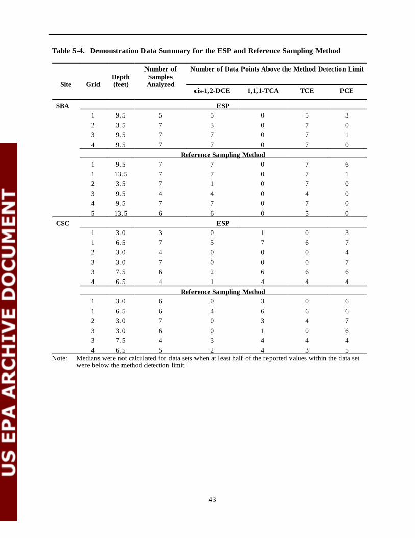
Table 5-4. Demonstration Data Summary for the ESP and Reference Sampling Method

Number of Number of Data Points Above the Method Detection Limit

Site Grid (feet)Depth

AnalyzedSamples

cis-1,2-DCE 1,1,1-TCA TCE PCE

SBA ESP 1 9.5 5 5 0 5 3 2 3.5 7 3 0 7 0 3 9.5 7 7 0 7 1 4 9.5 7 7 0 7 0

Reference Sampling Method 1 9.5 7 7 0 7 6 1 13.5 7 7 0 7 1 2 3.5 7 1 0 7 0 3 9.5 4 4 0 4 0 4 9.5 7 7 0 7 0 5 13.5 6 6 0 5 0

CSC ESP1 3.0 3 0 1 0 3 1 6.5 7 5 7 6 7 2 3.0 4 0 0 0 4 3 3.0 7 0 0 0 7 3 7.5 6 2 6 6 6 4 6.5 4 1 4 4 4

Reference Sampling Method 1 3.0 6 0 3 0 6 1 6.5 6 4 6 6 6 2 3.0 7 0 3 4 7 3 3.0 6 0 1 0 6 3 7.5 4 3 4 4 4 4 6.5 5 2 4 3 5

Note: Medians were not calculated for data sets when at least half of the reported values within the data setwere below the method detection limit.

43

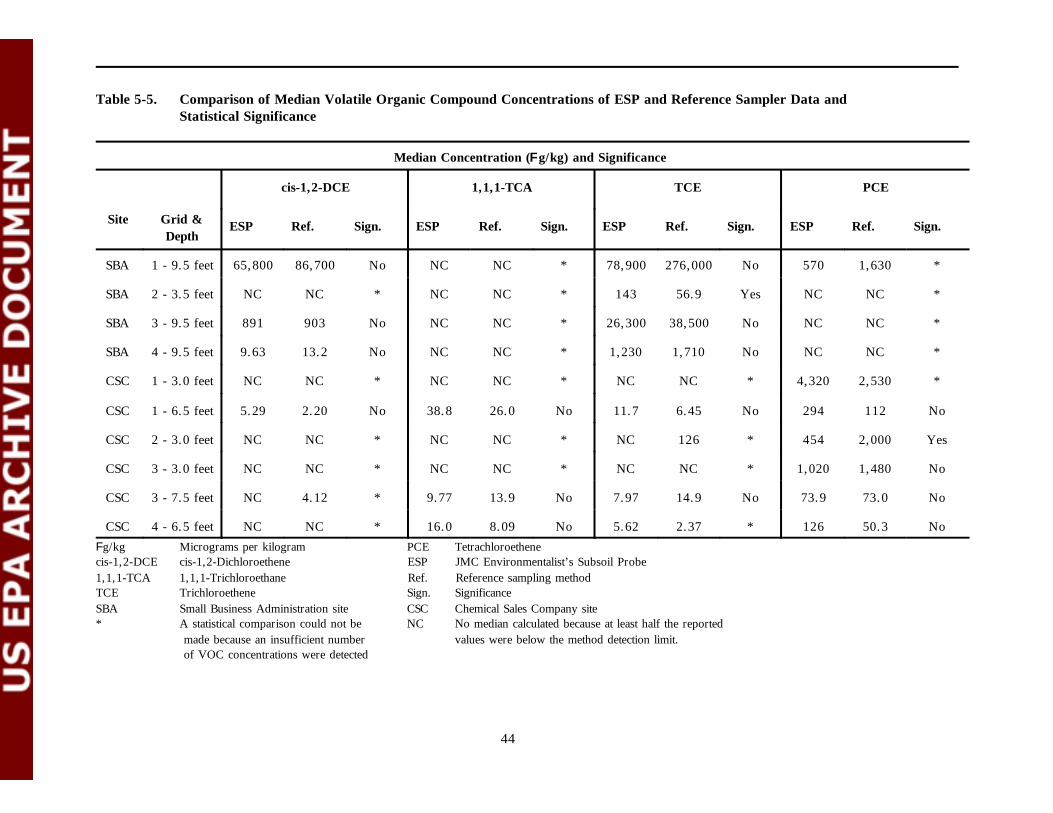
Table 5-5. Comparison of Median Volatile Organic Compound Concentrations of ESP and Reference Sampler Data and Statistical Significance

Median Concentration (F g/kg) and Significance

Site Grid & Depth

ESP

cis-1,2-DCE

Ref. Sign. ESP

1,1,1-TCA

Ref. Sign. ESP

TCE

Ref. Sign. ESP

PCE

Ref. Sign.

SBA

SBA

SBA

SBA

CSC

CSC

CSC

CSC

CSC

CSC

1 - 9.5 feet

2 - 3.5 feet

3 - 9.5 feet

4 - 9.5 feet

1 - 3.0 feet

1 - 6.5 feet

2 - 3.0 feet

3 - 3.0 feet

3 - 7.5 feet

4 - 6.5 feet

65,800

NC

891

9.63

NC

5.29

NC

NC

NC

NC

86,700 No

NC *

903 No

13.2 No

NC *

2.20 No

NC *

NC *

4.12 *

NC *

NC

NC

NC

NC

NC

38.8

NC

NC

9.77

16.0

NC

NC

NC

NC

NC

26.0

NC

NC

13.9

8.09

*

*

*

*

*

No

*

*

No

No

78,900

143

26,300

1,230

NC

11.7

NC

NC

7.97

5.62

276,000

56.9

38,500

1,710

NC

6.45

126

NC

14.9

2.37

No

Yes

No

No

*

No

*

*

No

*

570

NC

NC

NC

4,320

294

454

1,020

73.9

126

1,630

NC

NC

NC

2,530

112

2,000

1,480

73.0

50.3

*

*

*

*

*

No

Yes

No

No

No Fg/kg Micrograms per kilogram PCE Tetrachloroethene cis-1,2-DCE cis-1,2-Dichloroethene ESP JMC Environmentalist’s Subsoil Probe 1,1,1-TCA 1,1,1-Trichloroethane Ref. Reference sampling method TCE Trichloroethene Sign. Significance SBA Small Business Administration site CSC Chemical Sales Company site * A statistical comparison could not be NC No median calculated because at least half the reported

made because an insufficient number values were below the method detection limit. of VOC concentrations were detected

44

45

1000000 CSC SiteSBA Site 1000000

Envi

ronm

enta

list's

Sub

soil

Prob

e M

edia

n

Envi

ronm

enta

list's

Sub

soil

Prob

e M

edia

n 100000100000

1000

10000

VO

C C

once

ntra

tion

(µg/

kg)

cis-1,2-DCE

TCE

PCE

1,1,1-TCA

VO

C C

once

ntra

tion

(µg/

kg)

10000

1000

100100

1010

1

1 10 100 1000 10000 100000 1000000 1 10 100 1000 10000 100000 1000000 1

Reference Sampling Method Reference Sampling Method

Median VOC Concentration (µg/kg) Median VOC Concentration (µg/kg)

Note: µg/kg = micrograms per kilogram

Figure 5-1. Comparative Plot of Median VOC Concentrations for the ESP and Reference Sampling Method at the SBA and CSC Sites

method median concentrations. The total number of pairs in which the median concentrations were higher with the ESP were then compared with the total number of pairs in which the median concentrations were higher with the reference sampling method. If no bias is present in the data sets, the probability of the total number of pairs for one or the other test method being higher is equivalent; that is, the probability of the number of pairs in which the median concentrations in the ESP are higher is equal to the probability of the number of pairs in which the median concentrations in the reference sampling method are higher. A binomial expansion was used to determine the exact probability of the number of data sets in which the median concentrations for the ESP and reference sampling method were higher. If the calculated probability is less than 5 percent (p < 0.05), then a significant difference is present between the ESP and reference sampling method.

The sign test data are provided in Table 5-6 and are summarized in Appendix A5, Table A5. At the CSC site, the calculated probability is greater than 0.05; therefore, the difference is not statistically significant. However, the calculated probability at the SBA site is less than 0.05 indicating that the ESP yielded results that, statistically, were significantly different than the results for the reference sampling method (probability of 3.1 percent). This result suggests that in sampling fine-grained soils, the reference sampling method tends to yield higher VOC concentrations than does the ESP.

Table 5-6. Sign Test Results for the ESP and the Reference Sampling Method

Number of Pairs in Which the Median Concentration is Higher than Other Method

Sampler SBA Site CSC Site

Reference Sampler 7 4

ESP 1 9

Total Comparisons 8 13

Calculated Probability 0.031 0.087

Sample Integrity

Seven integrity samples were collected with the ESP in Grid 1 at the SBA site and five integrity samples were collected in Grid 1 at the CSC site, as described in Chapter 3, to determine if potting soil in a lined sampler interior became contaminated after it was advanced through a zone of high VOC concentrations. For the ESP, VOCs were detected in two of the 12 integrity samples: two at the SBA site and none at the CSC site. One of the integrity samples collected at the SBA site contained cis-1,2-DCE at 5,700 Fg/kg, TCE at 4,070 Fg/kg, and PCE at 212 Fg/kg; the other sample contained cis-1,2-DCE at 114 Fg/kg and TCE at 3.17 Fg/kg. These results indicate that the integrity of a lined chamber of the ESP may not be preserved when the sampler is advanced through highly contaminated soils. Results of sample integrity tests for the reference method indicate no contamination in the potting soil after advancement through a zone of high VOC concentrations. Because potting soil has an organic carbon content many times greater than typical soils, the integrity tests represent a worst-case scenario for VOC absorbance and may not be representative of cross-contamination under normal field conditions.

46

Sample Throughput

Sample retrieval time was measured as the amount of time required to set up at a sampling point, collect the specified sample, backfill the hole with granular bentonite, decontaminate the sampling equipment, and move to a new sampling location. The average retrieval time for the ESP was 36.9 minutes per sample at the SBA site using a single operator and 22.5 minutes per sample when two operators were used. Two operators were used for all grids sampled at the CSC site, resulting in an average sample retrieval time of 13.4 minutes per sample. Table 5-7 presents a comparison of the average sample retrieval times for the ESP to those for the reference sampling method. The average sample retrieval times for the ESP (when two operators were used) were slightly quicker than the reference sampling method in the clay soils at the SBA site. However, the retrieval times for the ESP were based on samples collected at 3.5, 6.5, and 9.5 feet bgs, while the average sample retrieval times for the reference method were calculated based on the amount of time required to sample these same target depths and two additional target depths not sampled using the ESP: the 13.5-foot depths at Grids 1 and 5. For this reason, the sample retrieval times for the ESP and the reference method may not be directly comparable for the SBA site. The average sample retrieval times for the ESP were slower than the reference sampling method when collecting samples at depths of 3.0, 6.5, and 7.5 feet in the sandy soils at the CSC site.

Data Quality

Data quality was assessed throughout this demonstration by implementing an approved quality assurance project plan (PRC, 1997). The QA/QC procedures included the consistent application of approved methods for sample collection, chemical analysis, and data reduction. Based on the intended use of the data, QA objectives for precision, accuracy, representativeness, comparability, and completeness were established and QC samples were collected to assess whether the QA objectives were met. Based on the results of a field audit conducted by the EPA and a detailed validation of the demonstration data by Tetra Tech, the ESP and reference sampling method data have been deemed acceptable for use as described in the demonstration design (Chapter 3). The results of the QC indicators selected for this demonstration for both the ESP and reference sampling method are provided in the Technology Evaluation Report for this demonstration (Tetra Tech, 1997) and are summarized in the data quality section of Chapter 4.

Table 5-7. Average Sample Retrieval Times for the ESP and the Reference Sampling Method

Average Sample Retrieval Time (minutes per sample)

Sampler SBA Site CSC Site

ESP 36.9 /22.5 a b 13.4b

Reference Sampling Method 26 8.4 Note: One- and two-person sampling crews collected soil samples using the ESP at the SBA and CSC sites, and

a three-person sampling crew collected soil samples using the reference sampling method at both sites.One additional person was present at the CSC site to direct drilling operations and assist with demonstration sampling, as necessary.

a One-person sampling crewb Two-person sampling crew

47

Chapter 6Economic Analysis

The ESP was demonstrated at two sites that varied geologically and were contaminated with VOCs at a range of concentrations. This chapter presents an economic analysis for applying the ESP at sites similar to those used in this demonstration. The demonstration costs for the reference sampling method are also provided.

The purpose of this economic analysis is to estimate the range of costs for using a Clements Associates, Inc., ESP to collect 42 subsurface soil samples at a clay soil site (400 feet total depth, similar to the SBA site) and a sandy soil site (200 feet total depth, similar to the CSC site). The analysis is based on the results and experience gained from this demonstration and on costs provided by Clements Associates, Inc. To account for variability in cost data and assumptions, the economic analysis is presented as a list of cost elements and a range of costs for collecting samples using the ESP.

Assumptions

Several factors affect the cost of subsurface soil sampling. Wherever possible, these factors are identified so that decision makers can independently complete a site-specific economic analysis. For example, this cost estimate is based on collecting soil samples from clay and sandy soil sites at sampling depths ranging from 3 feet bgs to 13.5 feet bgs and using the average sample retrieval times calculated during the demonstrations of 22.5 minutes per sample for the clay soil site and 13.4 minutes per sample at the sandy soil site. This cost estimate assumes that manual methods are used to advance the ESP and a hollow-stem auger drilling platform is used to advance the reference method. The cost estimate also assumes that minimal operator training is required for the ESP (less than one hour).

JMC Environmentalist’s Subsoil Probe

Costs for implementing the ESP are presented in two categories: (1) sampling equipment costs, which may include sampler purchase or rental costs and daily equipment use costs, and (2) operating and oversight costs, which include labor costs for sampling and other direct costs such as equipment shipping, supplies, IDW disposal, and site restoration.

The cost categories and associated cost elements are defined and discussed below and serves as the basis for the estimate cost ranges presented in Table 6-1.

Sampling Equipment Costs. This cost category accounts for obtaining the ESP sampling equipment required to extract soil samples from the subsurface and for daily equipment use. The ESP can either be purchased or rented.

48

Table 6-1. Estimated Subsurface Soil Sampling Costs for the JMC Environmentalist’s Subsoil Probe

Sampling Equipment Costs

ESP Sampler Purchase = $2,780ESP Sampler Rental = $250 per day

Daily Equipment Use (Optional) = $150 to $300 per day

Operating and Oversight Costs

Clay Soil Site Sandy Soil Site Total Sampling Time = 15 to 19 hours (2 days) Total Sampling Time = 9 to 11 hours (1 day)

Total Samples Collected = 42 Total Samples Collected = 42Total Sample Depth = 400 feet Total Sample Depth = 200 feetSample Crew Size = 2 People Sample Crew Size = 2 People

Labor Costs Labor Costs Mobilization/Demobilization $600 - $1,000 Mobilization/Demobilization $600 - $1,000 Travel $6 - $30 Travel $6 - $30 Per Diem 0 - $600 Per Diem 0 - $300 Sample Collection and $1,500 - $1,900 Sample Collection and Oversight $900 - $1,100 Oversight

Other Direct Costs Other Direct Costs Equipment Shipping $50 - $100 Equipment Shipping $50 - $100 Supplies $25 - $75 Supplies $25 - $75 IDW Disposal $200 - $300 IDW Disposal $200 - $300 Site Restoration $100 - $200 Site Restoration $100 - $200

Range of Operating and $2,480 - $4,210 $1,880 - $3,110 Oversight Costs*

* The range of Operating and Oversight Costs is rounded to the nearest tens of dollars and does not include Sampling Equipment Costs.

C Purchase Cost — The ESP purchase cost is estimated to be $2,780, which includes the ESP sampler and 15 liners ($1,826), one master extension rod ($187), six 36-inch extension rods for collecting samples at 20 feet bgs ($107 each), and 30 36-inch plastic liners ($63.55 for 15 liners).

C Rental Cost — The ESP rental cost from Clements Associates, Inc. is $250 per day. Sampler rental includes the ESP, one master extension rod, and six 36-inch extension rods. However, plastic liners must be purchased at an additional cost of $191 ($63.55 for 15 liners).

C Daily Equipment Use Costs — Daily equipment costs are estimated to range from $150 to $300 per day for the optional electric hammer and an 1,850-watt generator.

49

Operating and Oversight Costs. Operating costs are segregated into labor costs and other direct costs, as follows:

Labor costs include mobilization/demobilization, travel, per diem, and sample collection and oversight.

C Mobilization/Demobilization Labor Costs — This cost element includes the time for two personnel to prepare for and travel to each site, set up and pack up equipment, and return from the field and includes 6 to 10 hours for each person at a rate of $50 per hour.

C Travel Costs — Travel costs for each site are limited to round-trip mileage costs and areestimated to be between 20 to 100 miles at a rate of $0.30 per mile.

C Per Diem Costs — This cost element includes food, lodging, and incidental expenses, and is estimated to range from zero (for a local site) to $150 per day per person for two people for 2 days at the clay soil site (2 days for sample collection, mobilization/demobilization, and site restoration), and for 1 day at the sandy soil site (1 day for sample collection, mobilization/ demobilization, and site restoration).

C Sample Collection and Oversight Labor Costs — On-site labor may include a registered geologist and another environmental scientist to operate the sample probe, collect samples, and oversee sample collection. The total number of people on site is two. Based on the average demonstration sample retrieval times, sample collection and oversight labor is estimated to be 15 to 19 hours each for two people at the clay soil site, and 9 to 11 hours each for two people at the sandy soil site. Labor rates are estimated at $50 per hour. This labor estimate includes time for decontamination and site restoration.

Other direct costs include equipment shipping, supplies, IDW disposal, and site restoration costs.

C Equipment Shipping — These costs include the cost of shipping the ESP to and from thesampling site and are estimated to range from $50 to $100.

C Supplies — This cost element includes decontamination supplies, such as buckets, soap, high­purity rinse water, and brushes, as well as personal protective equipment (Level D, the minimum level of protection, is assumed). Supplies are estimated to cost between $25 and $75.

• IDW Disposal — Disposal costs for each site are limited to the cost of disposing one 55-gallon drum of IDW for $200 to $300 (typically, the minimum IDW disposal unit is one 55-gallon drum). Limited volumes of IDW were generated during the demonstration using the ESP because of the direct-push nature of the sampler advancement unit. No costs are included for wastewater disposal.

C Site Restoration — Site restoration costs include grouting the sample boreholes and site restoration labor. Grouting costs for each site are limited to grout and grouting tools and are estimated to range from $100 to $200.

Reference Sampling Method

The costs for implementing the reference sampling method during the demonstration include driller’s costs and oversight costs, as presented in Table 6-2 and discussed below.

50

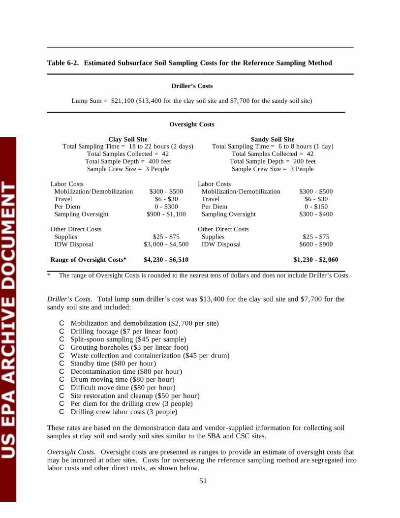
Table 6-2. Estimated Subsurface Soil Sampling Costs for the Reference Sampling Method

Driller’s Costs

Lump Sum = $21,100 ($13,400 for the clay soil site and $7,700 for the sandy soil site)

Oversight Costs

Clay Soil Site Sandy Soil SiteTotal Sampling Time = 18 to 22 hours (2 days) Total Sampling Time = 6 to 8 hours (1 day)

Total Samples Collected = 42 Total Samples Collected = 42Total Sample Depth = 400 feet Total Sample Depth = 200 feetSample Crew Size = 3 People Sample Crew Size = 3 People

Labor Costs Labor Costs Mobilization/Demobilization $300 - $500 Mobilization/Demobilization $300 - $500 Travel $6 - $30 Travel $6 - $30 Per Diem 0 - $300 Per Diem 0 - $150 Sampling Oversight $900 - $1,100 Sampling Oversight $300 - $400

Other Direct Costs Other Direct Costs Supplies $25 - $75 Supplies $25 - $75 IDW Disposal $3,000 - $4,500 IDW Disposal $600 - $900

Range of Oversight Costs* $4,230 - $6,510 $1,230 - $2,060

* The range of Oversight Costs is rounded to the nearest tens of dollars and does not include Driller’s Costs.

Driller’s Costs. Total lump sum driller’s cost was $13,400 for the clay soil site and $7,700 for the sandy soil site and included:

C Mobilization and demobilization ($2,700 per site) C Drilling footage ($7 per linear foot) C Split-spoon sampling ($45 per sample) C Grouting boreholes ($3 per linear foot) C Waste collection and containerization ($45 per drum) C Standby time ($80 per hour) C Decontamination time ($80 per hour) C Drum moving time ($80 per hour) C Difficult move time ($80 per hour) C Site restoration and cleanup ($50 per hour) C Per diem for the drilling crew (3 people) C Drilling crew labor costs (3 people)

These rates are based on the demonstration data and vendor-supplied information for collecting soil samples at clay soil and sandy soil sites similar to the SBA and CSC sites.

Oversight Costs. Oversight costs are presented as ranges to provide an estimate of oversight costs that may be incurred at other sites. Costs for overseeing the reference sampling method are segregated into labor costs and other direct costs, as shown below.

51

Labor costs include mobilization/demobilization, travel, per diem, and sampling oversight costs.

C Mobilization/Demobilization Labor Costs — This cost element includes the time for one person to prepare for and travel to each site, set up and pack up equipment, and return from the field and includes 6 to 10 hours at a rate of $50 per hour.

C Travel Costs — Travel costs for each site are limited to round-trip mileage costs and areestimated to be between 20 to 100 miles at a rate of $0.30 per mile.

C Per Diem Costs — This cost element includes food, lodging, and incidental expenses, and is estimated to range from zero (for a local site) to $150 per day per person for one person for 2 days at the clay soil site (2 days for sample collection, mobilization/demobilization and site restoration), and one person for 1 day at the sandy soil site (1 day for sample collection, mobilization/ demobilization, and site restoration).

C Sampling Oversight Labor Costs — On-site labor, often a registered geologist, is required to oversee sample collection. This cost element does not include the drill crew, which is covered in the lump sum driller’s cost. Based on the average demonstration sample retrieval times, oversight labor is estimated to be 18 to 22 hours for one person at the clay soil site, and 6 to 8 hours for one person at the sandy soil site. Labor rates are estimated at $50 per hour.

Other direct costs include supplies and IDW disposal.

C Supplies — This cost element includes personal protective equipment (Level D, the minimum level of protection, is assumed) and other miscellaneous field supplies. Supplies are estimated to cost between $25 and $75.

C IDW Disposal — Disposal costs for each site are limited to the cost of disposing of 15 55-gallon drums for the clay soil site and three 55-gallon drums for the sandy soil site at a cost of $200 to $300 per drum.

52

Chapter 7Summary of Demonstration Results

This chapter summarizes the technology performance results. The Clements Associates, Inc. ESP was compared to a reference subsurface soil sampling method (hollow-stem auger drilling and split-spoon sampling) in terms of the following parameters: (1) sample recovery, (2) VOC concentrations in recovered samples, (3) sample integrity, (4) reliability and throughput, and (5) cost.

The demonstration data indicate the following performance characteristics for the ESP:

C Sample Recovery: For the purposes of this demonstration, sample recovery was defined as the ratio of the length of recovered sample to the length of sampler advancement. Sample recoveries from 28 samples collected at the SBA site ranged from 42 to 100 percent, with an average sample recovery of 96 percent. Sample recoveries from 42 samples collected at the CSC site ranged from 72 to 100 percent, with an average sample recovery of 95 percent. Using the reference method, sample recoveries from 42 samples collected at the SBA site ranged from 40 to 100 percent, with an average recovery of 88 percent. Sample recoveries from the 41 samples collected at the CSC site ranged from 53 to 100 percent, with an average recovery of 87 percent. A comparison of recovery data from the ESP sampler and the reference sampler indicates that the ESP achieved higher sample recoveries in both the clay soil at the SBA site and in the sandy soil at the CSC site relative to the sample recoveries achieved by the reference sampling method.

C Volatile Organic Compound Concentrations: Soil samples collected using the ESP and the reference sampling method at five sampling depths in eight grids (four at the SBA site and four at the CSC site) were analyzed for VOCs. For 16 of the 18 ESP and reference sampling method pairs (seven at the SBA site and 11 at the CSC site), a statistical analysis using the Mann-Whitney test indicated no significant statistical difference at the 95 percent level between VOC concentrations in samples collected with the ESP and those collected with the reference sampling method. A statistically significant difference was identified for one sample pair collected at the SBA site and one sample pair at the CSC site. Analysis of the CSC site data, using the sign test, indicated no statistical difference between the data obtained by the ESP and the reference sampling method. However, at the SBA site, the sign test indicated that the data obtained by the ESP are statistically significantly different than the data obtained by the reference sampling method, suggesting that the reference method tends to yield higher concentrations in sampling fine-grained soils than does the ESP.

C Sample Integrity: Seven integrity samples were collected with each sampling method at the SBA site, and five integrity samples were collected with each sampling method at the CSC site to determine if potting soil in a lined sampler became contaminated after it was advanced through a zone of high VOC concentrations. For the ESP, VOCs were detected in two of the

53

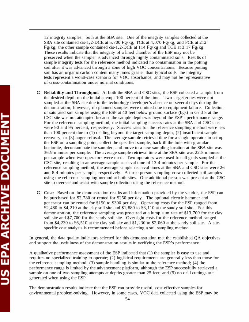
12 integrity samples: both at the SBA site. One of the integrity samples collected at the SBA site contained cis-1,2-DCE at 5,700 Fg/kg, TCE at 4,070 Fg/kg, and PCE at 212 Fg/kg; the other sample contained cis-1,2-DCE at 114 Fg/kg and TCE at 3.17 Fg/kg. These results indicate that the integrity of a lined chamber of the ESP may not be preserved when the sampler is advanced through highly contaminated soils. Results of sample integrity tests for the reference method indicated no contamination in the potting soil after it was advanced through a zone of high VOC concentrations. Because potting soil has an organic carbon content many times greater than typical soils, the integrity tests represent a worst-case scenario for VOC absorbance, and may not be representative of cross-contamination under normal conditions.

C Reliability and Throughput: At both the SBA and CSC sites, the ESP collected a sample from the desired depth on the initial attempt 100 percent of the time. Two target zones were not sampled at the SBA site due to the technology developer’s absence on several days during the demonstration; however, no planned samples were omitted due to equipment failure. Collection of saturated soil samples using the ESP at 40 feet below ground surface (bgs) in Grid 5 at the CSC site was not attempted because the sample depth was beyond the ESP’s performance range. For the reference sampling method, the initial sampling success rates at the SBA and CSC sites were 90 and 95 percent, respectively. Success rates for the reference sampling method were less than 100 percent due to (1) drilling beyond the target sampling depth, (2) insufficient sample recovery, or (3) auger refusal. The average sample retrieval time for a single operator to set up the ESP on a sampling point, collect the specified sample, backfill the hole with granular bentonite, decontaminate the sampler, and move to a new sampling location at the SBA site was 36.9 minutes per sample. The average sample retrieval time at the SBA site was 22.5 minutes per sample when two operators were used. Two operators were used for all grids sampled at the CSC site, resulting in an average sample retrieval time of 13.4 minutes per sample. For the reference sampling method, the average sample retrieval times at the SBA and CSC sites were 26 and 8.4 minutes per sample, respectively. A three-person sampling crew collected soil samples using the reference sampling method at both sites. One additional person was present at the CSC site to oversee and assist with sample collection using the reference method.

C Cost: Based on the demonstration results and information provided by the vendor, the ESP can be purchased for $2,780 or rented for $250 per day. The optional electric hammer and generator can be rented for $150 to $300 per day. Operating costs for the ESP ranged from $2,480 to $4,210 at the clay soil site and $1,880 to $3,110 at the sandy soil site. For this demonstration, the reference sampling was procured at a lump sum rate of $13,700 for the clay soil site and $7,700 for the sandy soil site. Oversight costs for the reference method ranged from $4,230 to $6,510 at the clay soil site and $1,230 to $2,060 at the sandy soil site. A site­specific cost analysis is recommended before selecting a soil sampling method.

In general, the data quality indicators selected for this demonstration met the established QA objectives and support the usefulness of the demonstration results in verifying the ESP’s performance.

A qualitative performance assessment of the ESP indicated that (1) the sampler is easy to use and requires no specialized training to operate; (2) logistical requirements are generally less than those for the reference sampling method; (3) sample handling is similar to the reference method; (4) the performance range is limited by the advancement platform, although the ESP successfully retrieved a sample on one of two sampling attempts at depths greater than 25 feet; and (5) no drill cuttings are generated when using the ESP.

The demonstration results indicate that the ESP can provide useful, cost-effective samples for environmental problem-solving. However, in some cases, VOC data collected using the ESP may be

54

statistically different from VOC data collected using the reference sampling method. Also, the integrity of a lined sample chamber may not be preserved when the sampler is advanced through highly contaminated clay soils. As with any technology selection, the user must determine what is appropriate for the application and project data quality objectives.

55

Chapter 8Technology Update

Clements Associates, Inc. has been in the business of manufacturing and selling hand-operated soil investigation equipment since 1972. The ESP system, used at the performance verification demonstration in June 1997, was developed initially to sample for agrichemical residues that contained radioactive trace elements.

The ESP has been used for a large range of environmental soil investigations. Its light weight and compact size mean that sampling personnel can carry it in the trunk of a passenger car or check it as airline baggage. This extreme portability and ease of use make the ESP a useful reconnaissance tool or, in many cases, the only subsurface investigation equipment of many consulting firms.

The ESP is being used in all of the United States, Canada, Mexico, Australia, Japan, Bolivia, England, and France. Units used in Bolivia were selected for use there by a large U.S.-based environmental consulting firm because of the simplicity, portability, and ease of operation. Much of the field work was done by local personnel having no previous sampling experience.

In addition to site assessment work, the ESP and the ESP Plus are used by agrichemical companies and agricultural research firms conducting soil dissipation or environmental fate studies as required by the EPA. The benefits are smaller plot sizes, the ability to sample regardless of surface ground conditions, ease of moving sampling equipment to remote locations or plots with limited access, and more efficient and more rapid sampling. Clements Associates, Inc. has developed a system of sampling tubes called Concentric Sampling Tubes for collecting the uppermost portion of the sample, which contains the highest amount of chemical contaminants.

The ESP Plus was developed to provide a larger volume of sample. It is of greater use in the soil dissipation arena.

Chapter 8 was written solely by Clements Associates, Inc. The statements presented in this chapter represent the vendor’s point of view and summarize the claims made by the vendor regarding the ESP. Publication of this material does not represent the EPA’s approval or endorsement of the statements made in this chapter; results of the performance evaluation of the ESP are discussed in other chapters of this report.

56

Chapter 9Previous Deployment

Although Clements Associates, Inc., claims that the ESP has been used widely throughout the United States and internationally, they chose not to provide additional information in this chapter on previous deployment of the ESP.

57

References

Bohn, H., Brian, M., and George, O. 1979. Soil Chemistry. John Wiley & Sons. New York, New York.

Central Mine Equipment Company. 1994. Augers Brochure. St. Louis, Missouri.

Clements Associates, Inc. 1997. Product Schematics.

Ecology & Environment. 1996. “Expanded Site Inspection for the Albert City, SBA Site, Albert City, Iowa.” July.

Engineering-Science, Inc. 1991. “Remedial Investigation/Feasibility Report for the Chemical Sales Company Superfund Site, OU1, Leyden Street Site.”

PRC Environmental Management, Inc. 1997. “Final Demonstration Plan for the Evaluation of Soil Sampling and Soil Gas Sampling Technologies.”

Rohlf, F. James and Robert R. Sokal. 1969. Statistical Tables. W. H. Freeman and Company. Table CC. Critical values of the Mann-Whitney statistic, page 241.

Terzaghi, Karl, and Ralph B. Peck. 1967. Soil Mechanics in Engineering Practice. John Wiley & Sons. New York, New York.

Tetra Tech EM Inc. 1997. “ Soil and Soil Gas Technology Evaluation Report.”

U.S. Environmental Protection Agency (EPA). 1986. Test Methods for Evaluating Solid Waste. SW-846. Third Edition.

EPA. 1987. “A Compendium of Superfund Field Operations Methods.” Office of Emergency and Remedial Response. Washington, DC. EPA 540-P-87 001. December.

58

APPENDIX A

DATA SUMMARY TABLES AND STATISTICAL METHODDESCRIPTIONS

FOR THE

CLEMENTS ASSOCIATES, INC.JMC ENVIRONMENTALIST’S SUBSOIL PROBE (ESP)

A-1

APPENDIX A1

STATISTICAL METHOD DESCRIPTIONS

MANN-WHITNEY TEST AND SIGN TEST

A-2

MANN-WHITNEY TEST

A statistical evaluation of the volatile organic compound (VOC) concentration data was conducted based on the null hypothesis that there is no difference between the median contaminant concentrations obtained by the Environmentalist’s Subsoil Probe (ESP) and the reference sampling method. The two-tailed significance level for this null hypothesis was set at a probability of 5 percent (p#0.05) (2.5 percent for a one-tailed); that is, if a two-tailed statistical analysis indicates a probability of greater than 5 percent that there is no significant difference between data sets, then it will be concluded that there is no significant difference between the data sets. A two-tailed test was used because no information was available to indicate a priori that one method would result in greater concentrations than the other method. Because the F test for homogeneity of variances failed, a parametric analysis of variance could not be used to test the hypothesis. Therefore, a nonparametric method, the Mann-Whitney test, was used to test the statistical hypothesis for VOC concentrations. The Mann-Whitney statistic makes no assumptions regarding normality and assumes only that the differences between two values, in this case the reported chemical concentrations, can be determined. Other assumptions required for use of the Mann-Whitney test are that samples are independent of each other and that the populations from which the samples are taken differ only in location. The Mann-Whitney test was chosen because of its historical acceptability and ease of application to small data sets.

To use the Mann-Whitney test, all of the data within two data sets that are to be compared are ranked without regard to the population from which each sample was withdrawn. The cis-1,2-dichloroethene (DCE) data from the SBA site are provided as an example in Table A1. The combined data from both data sets are ranked from the lowest value to the highest. Next, the sum of ranks within a sample set is determined by adding the assigned rank values. In the example provided in Table A1, the sum of ranks is 26 for the ESP data and 52 for the reference sampling methods.

A Mann-Whitney statistic is then calculated for each data set as follows:

Mann-Whitney = N N + N 1 1 2 1(N1 +1) - sum of ranks value for the first data set 2

and

Mann-Whitney = N N + N 2 1 2 2(N2 +1) - sum of ranks value for the second data set 2

Where

N is the number of values in data set 11 N is the number of values in data set 22

A-3

Table A1. Mann-Whitney Test Rank of cis-1,2-DCE Data from the 9.5 Foot Depth of Grid 1 at the SBA Site

cis-1,2-DCE cis-1,2-DCE Median Sample Concentration Concentration Value

Sampler Location (mg/kg) Rank Rank

ESP A5 182 12 5

ESP B1 22.3 1 1

ESP E7 65.8 5 3

ESP F3 66.1 6 4

ESP G5 23.2 2 2

Reference A3 49.7 3 1

Reference B2 86.7 8 4

Reference C2 109 10 6

Reference D4 147 11 7

Reference E4 67.1 7 3

Reference F2 98.4 9 5

Reference G7 50.2 4 2

Sum of ESP Ranks 26 (12+1+5+6+2 = 26)

Sum of Reference Sampler Ranks 52 (3+8+10+11+7+9+4 = 52)

Mann-Whitney Statistic 241

Mann-Whitney Statistic 112

Critical Mann-Whitney Value (for N=7, N =7, p=0.05) 301 2

Significance (Mann-Whitney Statistic > 30 ?) no

A-4

For the example provided in Table A1, the equations become:

Mann-Whitney = (7)(5) + 5(5+1) - 262 2

Mann-Whitney = 35 + 15 - 262

Mann-Whitney = 242

and

Mann-Whitney = (7)(5) + 7(7+1) - 521 2

Mann-Whitney = 35 + 28 - 521

Mann-Whitney = 111

To determine the significance of the calculated Mann-Whitney value, a table of critical values for the Mann-Whitney statistic is consulted. For the case of 7 samples in each data set, the Mann-Whitney statistic value for N =7 and N =5 is of interest. For a two-tailed test with a significance level of1 2 0.05, the Mann-Whitney statistic value is 30 (Rohlf and Sokal, 1969). Therefore, when the Mann-Whitney statistic value is greater than 30, a significance level of p < 0.05 has been realized, and the null hypothesis is rejected; that is, the two data sets are statistically different. The example comparison provided in Table A1 yielded a maximum Mann-Whitney statistic of 24, which is less than 30; therefore, there is no statistically significant difference between the two data sets, and the null hypothesis is accepted.

The question of data points with equal values may be easily addressed with the Mann-Whitney statistic. When two values (contaminant concentrations in this instance) are equivalent, the median rank is assigned to each. For instance, if the initial two values in the rank series are equivalent (regardless of which data set they were derived from) they would be assigned a median rank of 1.5 ([1+2]/2 = 1.5). For three equivalent ranks, the assigned rank for each value would be 2 ([1+2+3]/3 = 2). This approach is also applied to data points where contaminant concentrations are reported as below the method detection limit.

For the demonstration data, certain VOCs were not detected in some, or all, of the samples for many data sets. There is no strict guidance regarding the appropriate number of values that must be reported within a data set to yield statistically valid results. Therefore, and for the purposes of this statistical analysis, the maximum number of nondetects allowed within any given data set has been set at three. That is, there must be at least four reported values above the method detection limit within each data set to perform the Mann-Whitney test.

A-5

SIGN TEST

The sign test was used to examine the potential for sampling and analytical bias between the ESP and the reference sampling method. The sign test is nonparametric and counts the number of positive and negative signs among the differences. The differences tested, in this instance, were the differences in the median concentrations of paired data sets (within a site, within a grid, within a depth, and within an analyte). From the data sets, counts were made of (1) the number of pairs in which the reference sampling method median concentrations were higher than the ESP median concentrations and (2) the number of pairs in which the ESP median concentrations were higher than the reference sampling method median concentrations. The total number of pairs in which the median concentrations were higher in ESP was then compared with the total number of pairs in which the median concentrations in the reference sampling method were higher. If no bias is present in the data sets, the probability that the total number of pairs for one or the other test method is higher is equivalent. That is, the probability of the number of pairs in which the median concentrations in the ESP are higher is equal to the probability of the number of pairs in which the median concentrations in the reference sampling method are higher. A binomial expansion was used to determine the exact probability of the number of data sets in which the median concentrations in the ESP and reference sampling method were higher. If the calculated probability is less then 5 percent (p < 0.05), then a significant difference is present between the ESP and reference sampling method.

The sign test was chosen because it (1) reduces sensitivity to random analysis error and matrix variabilities by using the median VOC concentration across each grid depth, (2) enlarges the sample sizes as compared to the Mann-Whitney test, and (3) is easy to use.

For the demonstration data, certain VOCs were not detected in some, or all of the samples for many data sets. There is no strict guidance regarding the appropriate number of values that must be reported within a data set to yield statistically valid results. Therefore, and for the purposes of the statistical analysis, the maximum number of nondetects allowed within any given data set has been set at three. That is, there must be four reported values within each data set to perform the sign test.

A-6

APPENDIX A2

SAMPLE RECOVERY TEST DATA

A-7

TABLE A2a. ENVIRONMENTALIST'S SUBSOIL PROBE SAMPLER RECOVERY TEST DATASBA SITE

Sample Number Sample

Location Soil Type Reported Length

Pushed (in.) Reported Length Recovered (in.)

Sample Recovery (%)

CLEAC1G509.5 G5 Fine 12.0 12.0 100.0% CLEAG1A509.5 A5 Fine 12.0 13.0 100.0%a

CLEAG1B109.5 B1 Fine 12.0 15.0 100.0%a

CLEAG1C309.5 C3 Fine 12.0 12.0 100.0% CLEAG1D709.5 D7 Fine 12.0 18.0 100.0%a

CLEAG1E109.5 E1 Fine 12.0 15.0 100.0%a

CLEAG1F309.5 F3 Fine 12.0 15.0 100.0%a

CLEAG2A603.5 A6 Fine 36.0 36.0 100.0% CLEAG2B103.5 B1 Fine 30.0 26.0 86.7% CLEAG2C603.5 C6 Fine 36.0 34.0 94.4% CLEAG2D403.5 D4 Fine 36.0 34.0 94.4% CLEAG2E303.5 E3 Fine 36.0 31.0 86.1% CLEAG2G103.5 G1 Fine 30.0 27.0 90.0% CLEAG2F603.5 F6 Fine 36.0 36.0 100.0% CLEAG3A509.5 A5 Fine 12.0 20.0 100.0%a

CLEAG3B309.5 B3 Fine 12.0 5.0 41.7% CLEAG3C209.5 C2 Fine 12.0 14.0 100.0%a

CLEAG3D509.5 D5 Fine 12.0 18.0 100.0%a

CLEAG3E409.5 E4 Fine 12.0 18.0 100.0%a

CLEAG3F109.5 F1 Fine 12.0 16.0 100.0%a

CLEAG3G309.5 G3 Fine 12.0 12.0 100.0% CLEAG4A709.5 A7 Fine 36.0 36.0 100.0% CLEAG4B609.5 B6 Fine 12.0 15.0 100.0%a

CLEAG4C209.5 C2 Fine 12.0 18.0 100.0%a

CLEAG4D509.5 D5 Fine 36.0 36.0 100.0% CLEAG4F709.5 F7 Fine 24.0 24.0 100.0% CLEAG4E209.5 E2 Fine 36.0 36.0 100.0% CLEAG4G509.5 G5 Fine 36.0 36.0 100.0%

a Sample recovery is reported as 100 percent when length recovered is greater than length pushed. Average: 96.2%

Range: 41.7% - 100%Total # Samples: 28

A-8

TABLE A2b. ENVIRONMENTALIST'S SUBSOIL PROBE SAMPLER RECOVERY TEST DATACSC SITE

Sample Number Sample Location Soil Type

Reported Length Pushed (in.)

Reported Length Recovered (in.)

Sample Recovery (%)

CLECG1A103.0 A1 Coarse 36.0 32.0 88.9% CLECG1B403.0 B4 Coarse 36.0 36.0 100.0% CLECG1C103.0 C1 Coarse 36.0 36.0 100.0% CLECG1D303.0 D3 Coarse 36.0 33.0 91.7% CLECG1E703.0 E7 Coarse 36.0 36.0 100.0% CLECG1F603.0 F6 Coarse 36.0 36.0 100.0% CLECG1G103.0 G1 Coarse 36.0 35.0 97.2% CLECG1A106.5 A1 Coarse 36.0 34.5 95.8% CLECG1B406.5 B4 Coarse 36.0 31.5 87.5% CLECG1C106.5 C1 Coarse 36.0 31.0 86.1% CLECG1D306.5 D3 Coarse 36.0 32.0 88.9% CLECG1E706.5 E7 Coarse 36.0 31.5 87.5% CLECG1F606.5 F6 Coarse 36.0 32.0 88.9% CLECG1G106.5 G1 Coarse 36.0 32.0 88.9% CLECG2A503.0 A5 Coarse 36.0 33.0 91.7% CLECG2C603.0 C6 Coarse 36.0 36.0 100.0% CLECG2F403.0 F4 Coarse 36.0 36.0 100.0% CLECG2E603.0 E6 Coarse 36.0 33.5 93.1% CLECG2B203.0 B2 Coarse 36.0 36.0 100.0% CLECG2D303.0 D3 Coarse 36.0 33.0 91.7% CLECG2G603.0 G6 Coarse 36.0 36.0 100.0% CLECG3A503.0 A5 Coarse 36.0 36.0 100.0% CLECG3B403.0 B4 Coarse 36.0 34.0 94.4% CLECG3C603.0 C6 Coarse 36.0 36.0 100.0% CLECG3D503.0 D5 Coarse 36.0 36.0 100.0% CLECG3E303.0 E3 Coarse 36.0 35.0 97.2% CLECG3F403.0 F4 Coarse 36.0 32.0 88.9% CLECG3G503.0 G5 Coarse 36.0 36.0 100.0% CLECG3A507.5 A5 Coarse 36.0 31.5 87.5% CLECG3B407.5 B4 Coarse 36.0 32.0 88.9% CLECG3C607.5 C6 Coarse 36.0 29.0 80.6% CLECG3D507.5 D5 Coarse 36.0 26.0 72.2% CLECG3E307.5 E3 Coarse 36.0 36.0 100.0% CLECG3F407.5 F4 Coarse 36.0 31.0 86.1% CLECG3G507.5 G5 Coarse 36.0 34.0 94.4% CLECG4A306.5 A3 Coarse 36.0 36.0 100.0% CLECG4B506.5 B5 Coarse 36.0 36.0 100.0% CLECG4C606.5 C6 Coarse 36.0 36.0 100.0% CLECG4D706.5 D7 Coarse 36.0 36.0 100.0% CLECG4E306.5 E3 Coarse 36.0 36.0 100.0% CLECG4F506.5 F5 Coarse 36.0 36.0 100.0% CLECG4G406.5 G4 Coarse 36.0 36.0 100.0%

Average: 94.5% Range: 72.2 - 100.0%

Total # Samples:

A-9

42

TABLE A2c. REFERENCE SAMPLING METHOD RECOVERY TEST DATASBA SITE

Sample Number Sample

Location Soil Type Reported Length

Pushed (in.) Reported Length Recovered (in.)

Sample Recovery (%)

REFAG1A309.5 A3 Fine 18.0 13.5 75.0% REFAG1A313.5 A3 Fine 19.0 17.0 89.5% REFAG1B209.5 B2 Fine 18.0 17.0 94.4% REFAG1B213.5 B2 Fine 18.0 19.0 100.0%a

REFAG1C209.5 C2 Fine 18.0 16.0 88.9% REFAG1C213.5 C2 Fine 18.0 11.0 61.1% REFAG1D409.5 D4 Fine 18.0 16.0 88.9% REFAG1D413.5 D4 Fine 18.0 17.5 97.2% REFAG1E409.5 E4 Fine 18.0 17.0 94.4% REFAG1E413.5 E4 Fine 18.0 17.0 94.4% REFAG1F209.5 F2 Fine 18.0 16.0 88.9% REFAG1F213.5 F2 Fine 18.0 17.0 94.4% REFAG1G709.5 G7 Fine 18.0 18.0 100.0% REFAG1G713.5 G7 Fine 18.0 16.0 88.9% REFAG2A203.5 A2 Fine 18.0 18.0 100.0% REFAG2B403.5 B4 Fine 18.0 14.0 77.8% REFAG2C103.5 C1 Fine 18.0 12.0 66.7% REFAG2D603.5 D6 Fine 18.0 9.0 50.0% REFAG2E503.5 E5 Fine 18.0 16.0 88.9% REFAG2F103.5 F1 Fine 18.0 18.0 100.0% REFAG2G403.5 G4 Fine 18.0 17.0 94.4% REFAG3A209.5 A2 Fine 15.0 20.0 100.0%a

REFAG3B609.5 B6 Fine 15.0 18.0 100.0%a

REFAG3C409.5 C4 Fine 15.0 6.0 40.0% REFAG3D609.5 D6 Fine 15.0 13.0 86.7% REFAG3E109.5 E1 Fine 15.0 16.5 100.0%a

REFAG3F309.5 F3 Fine 15.0 21.0 100.0%a

REFAG3G609.5 G6 Fine 18.0 24.0 100.0%a

REFAG4A109.5 A1 Fine 18.0 16.5 91.7% REFAG4B309.5 B3 Fine 18.0 18.0 100.0% REFAG4C309.5 C3 Fine 18.0 16.0 88.9% REFAG4D609.5 D6 Fine 18.0 17.0 94.4% REFAG4E709.5 E7 Fine 18.0 17.0 94.4% REFAG4F209.5 F2 Fine 18.0 15.0 83.3% REFAG4G209.5 G2 Fine 18.0 17.5 97.2% REFAG5A213.5 A2 Fine 18.0 18.0 100.0% REFAG3B113.5 B1 Fine 18.0 18.0 100.0% REFAG5C213.5 C2 Fine 18.0 15.5 86.1% REFAG5D613.5 D6 Fine 18.0 17.0 94.4% REFAG5E313.5 E3 Fine 18.0 11.0 61.1% REFAG5F313.5 F3 Fine 18.0 12.0 66.7% REFAG5G413.5 G4 Fine 18.0 17.0 94.4%

a Sample recovery is reported as 100 percent when length recovered is greater than length pushed. Average: 88.4%

Range: 40.0-100.0% Total # Samples:

A-10

42

TABLE A2d. REFERENCE SAMPLING METHOD RECOVERY TEST DATACSC SITE

Sample Number Sample

Location Soil Type Reported Length

Pushed (in.) Reported Length Recovered (in.)

Sample Recovery (%)

REFCG1A303.0 A3 Coarse 18.0 12.0 66.7% REFCG1A306.5 A3 Coarse 18.0 16.0 88.9% REFCG1B303.0 B3 Coarse 18.0 10.0 55.6% REFCG1B306.5 B3 Coarse 18.0 14.0 77.8% REFCG1C303.0 C3 Coarse 18.0 15.0 83.3% REFCG1C306.5 C3 Coarse 18.0 13.0 72.2% REFCG1D503.0 D5 Coarse 18.0 16.0 88.9% REFCG1D506.5 D5 Coarse 18.0 14.0 77.8% REFCG1E103.0 E1 Coarse 18.0 20.0 100.0%a

REFCG1E106.5 E1 Coarse 18.0 11.5 63.9% REFCG1F103.0 F1 Coarse 18.0 14.5 80.6% REFCG1F106.5 F1 Coarse 18.0 15.0 83.3% REFCG1G703.0 G7 Coarse 18.0 14.0 77.8% REFCG1G706.5 G7 Coarse 18.0 15.0 83.3% REFCG2A103.0 A1 Coarse 18.0 13.0 72.2% REFCG2B603.0 B6 Coarse 18.0 19.0 100.0%a

REFCG2C103.0 C1 Coarse 18.0 16.0 88.9% REFCG2D603.0 D6 Coarse 18.0 18.0 100.0% REFCG2E303.0 E3 Coarse 18.0 19.5 100.0%a

REFCG2F503.0 F5 Coarse 18.0 18.5 100.0%a

REFCG2G103.0 G1 Coarse 19.0 19.0 100.0% REFCG3A203.0 A2 Coarse 18.0 17.5 97.2% REFCG3A207.5 A2 Coarse 18.0 12.0 66.7% REFCG3B103.0 B1 Coarse 18.0 17.0 94.4% REFCG3B107.5 B1 Coarse 18.0 12.0 66.7% REFCG3C203.0 C2 Coarse 18.0 18.0 100.0% REFCG3C207.5 C2 Coarse 18.0 9.5 52.8% REFCG3D603.0 D6 Coarse 19.0 18.0 94.7% REFCG3D607.5 D6 Coarse 20.0 20.0 100.0% REFCG3E603.0 E6 Coarse 18.0 18.0 100.0% REFCG3E607.5 E6 Coarse 18.0 18.0 100.0% REFCG3F603.0 F6 Coarse 18.0 18.0 100.0% REFCG3F607.5 F6 Coarse No data No data --REFCG3G403.0 G4 Coarse 18.0 17.0 94.4% REFCG3G407.5 G4 Coarse 18.0 18.0 100.0% REFCG4A706.5 A7 Coarse 18.0 18.0 100.0% REFCG4B606.5 B6 Coarse 18.0 13.0 72.2% REFCG4C706.5 C7 Coarse 18.0 17.0 94.4% REFCG4D306.5 D3 Coarse 18.0 17.0 94.4% REFCG4E506.5 E5 Coarse 18.0 18.0 100.0% REFCG4F306.5 F3 Coarse 18.0 18.0 100.0% REFCG4G506.5 G5 Coarse 18.0 11.5 63.9%

a Sample recovery is reported as 100 percent when length recovered is greater than length pushed. Average: 86.7%

Range: 52.8-100.0% Total # Samples:

A-11

41

APPENDIX A3

VOLATILE ORGANIC COMPOUND CONCENTRATIONS

A-12

TABLE A3a. VOLATILE ORGANIC COMPOUND CONCENTRATIONSFOR ENVIRONMENTALIST'S SUBSOIL PROBE SAMPLER AND REFERENCE SAMPLING METHOD

SBA SITE - GRID 1 - 9.5 FEET

A-13

Sample Name

Sample Location

Soil Type

Concentration Zone

Contaminant Concentration (mg/kg) cis-1,2-DCE 1,1,1-TCA TCE PCE

ENVIRONMENTALIST'S SUBSOIL PROBE SAMPLER DATA CLEAG1A509.5 A5 Fine High 182,441 100 63,996 570 CLEAG1B109.5 B1 Fine High 22,319 100 53,779 100 CLEAG1E709.5 E7 Fine High 65,819 100 454,575 3,622 CLEAG1F309.5 F3 Fine High 66,130 100 551,013 2,357 CLEAG1G509.5 G5 Fine High 23,237 100 78,916 100

Range: 22,300 - 182,000 100 53,800 - 551,000 100 - 3,620

Median: 65,800 NC 78,900 570

REFERENCE SAMPLING METHOD DATA REFAG1A309.5 A3 Fine High 49,671 100 52,846 100 REFAG1B209.5 B2 Fine High 86,749 100 70,217 669 REFAG1C209.5 C2 Fine High 108,582 100 251,269 2,012 REFAG1D409.5 D4 Fine High 147,042 100 418,733 4,511 REFAG1E409.5 E4 Fine High 67,126 100 290,739 1,534 REFAG1F209.5 F2 Fine High 98,437 100 276,149 1,720 REFAG1G709.5 G7 Fine High 50,237 100 289,330 1,625

Range: 49,700 - 147,000 100 52,800 - 419,000 100 - 4,510

Median: 86,700 NC 276,000 1,630

Note: NC =

mg/kg =

Values reported as "100" are nondetects with a detection limit of 100. No medians calculated because at least half the reported values were below the method detection limit. Micrograms per kilogram.

TABLE A3b. VOLATILE ORGANIC COMPOUND CONCENTRATIONSFOR ENVIRONMENTALIST'S SUBSOIL PROBE SAMPLER AND REFERENCE SAMPLING METHOD

SBA SITE - GRID 1 - 13.5 FEET

A-14

Sample Name

Sample Location

Soil Type

Concentration Zone

Contaminant Concentration (mg/kg) cis-1,2-DCE 1,1,1-TCA TCE PCE

ENVIRONMENTALIST'S SUBSOIL PROBE SAMPLER DATA

ENVIRONMENTALISTS'S SUBSOIL PROBE SAMPLER DATA NOT COLLECTED

Range:

Median:

REFERENCE SAMPLING METHOD DATA REFAG5A213.5 A2 Fine High 6,762 100 33,736 100 REFAG5C213.5 C2 Fine High 14,453 100 40,511 100 REFAG5C213.5D C2 Fine High 20,362 100 48,730 100 REFAG5D613.5 D6 Fine High 44,929 100 432,508 2,405 REFAG5E313.5 E3 Fine High 12,343 100 40,984 100 REFAG5F313.5 F3 Fine High 15,415 100 26,652 100 REFAG5G413.5 G4 Fine High 1,356 100 39,138 100

Range: 1,360 - 44,900 100 26,700 - 433,000 100

Median: 14,500 NC 40,500 NC

Note: NC =

mg/kg =

Values reported as "100" are nondetects with a detection limit of 100. No medians calculated because at least half the reported values were below the method detection limit. Micrograms per kilogram.

TABLE A3c. VOLATILE ORGANIC COMPOUND CONCENTRATIONSFOR ENVIRONMENTALIST'S SUBSOIL PROBE SAMPLER AND REFERENCE SAMPLING METHOD

SBA SITE - GRID 2 - 3.5 FEET

A-15

Sample Name

Sample Location

Soil Type

Concentration Zone

Contaminant Concentration (mg/kg) cis-1,2-DCE 1,1,1-TCA TCE PCE

ENVIRONMENTALIST'S SUBSOIL PROBE SAMPLER DATA CLEAG2A603.5 A6 Fine Low 3.42 1 328 1 CLEAG2B103.5 B1 Fine Low 1 1 37.4 1 CLEAG2C603.5 C6 Fine Low 1 1 159 1 CLEAG2D403.5 D4 Fine Low 1 1 71.0 1 CLEAG2E303.5 E3 Fine Low 3.08 1 143 1 CLEAG2F603.5 F6 Fine Low 1 1 109 1 CLEAG2G103.5 G1 Fine Low 4.34 1 155 1

Range: 1 - 4.34 1 37.4 - 328 1

Median: NC NC 143 NC

REFERENCE SAMPLING METHOD DATA REFAG2A203.5 A2 Fine Low 1 1 22.6 1 REFAG2B403.5 B4 Fine Low 1 1 58.2 1 REFAG2C103.5 C1 Fine Low 1 1 29.3 1 REFAG2D603.5 D6 Fine Low 1 1 43.5 1 REFAG2E503.5 E5 Fine Low 1 1 56.9 1 REFAG2F103.5 F1 Fine Low 1 1 78.6 1 REFAG2G403.5 G4 Fine Low 2.18 1 88.8 1

Range: 1 - 2.18 1 22.6 - 88.8 1

Median: NC NC 56.9 NC

Note: NC =

mg/kg =

Values reported as "1" are nondetects with a detection limit of 1. No medians calculated because at least half the reported values were below the method detection limit. Micrograms per kilogram.

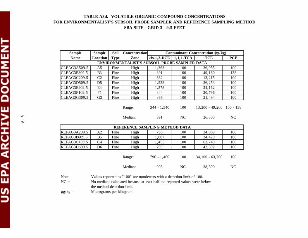
TABLE A3d. VOLATILE ORGANIC COMPOUND CONCENTRATIONSFOR ENVIRONMENTALIST'S SUBSOIL PROBE SAMPLER AND REFERENCE SAMPLING METHOD

SBA SITE - GRID 3 - 9.5 FEET

A-16

Sample Name

Sample Location

Soil Type

Concentration Zone

Contaminant Concentration (mg/kg) cis-1,2-DCE 1,1,1-TCA TCE PCE

ENVIRONMENTALIST'S SUBSOIL PROBE SAMPLER DATA CLEAG3A509.5 A5 Fine High 1,363 100 36,955 100 CLEAG3B309.5 B3 Fine High 891 100 49,180 138 CLEAG3C209.5 C2 Fine High 662 100 13,215 100 CLEAG3D509.5 D5 Fine High 1,538 100 26,253 100 CLEAG3E409.5 E4 Fine High 1,378 100 24,162 100 CLEAG3F109.5 F1 Fine High 344 100 20,796 100 CLEAG3G309.5 G3 Fine High 366 100 31,494 100

Range: 344 - 1,540 100 13,200 - 49,200 100 - 138

Median: 891 NC 26,300 NC

REFERENCE SAMPLING METHOD DATA REFAG3A209.5 A2 Fine High 796 100 34,069 100 REFAG3B609.5 B6 Fine High 1,007 100 34,420 100 REFAG3C409.5 C4 Fine High 1,455 100 63,740 100 REFAG3D609.5 D6 Fine High 799 100 42,502 100

Range: 796 - 1,460 100 34,100 - 63,700 100

Median: 903 NC 38,500 NC

Note: NC =

mg/kg =

Values reported as "100" are nondetects with a detection limit of 100. No medians calculated because at least half the reported values were below the method detection limit. Micrograms per kilogram.

TABLE A3e. VOLATILE ORGANIC COMPOUND CONCENTRATIONSFOR ENVIRONMENTALIST'S SUBSOIL PROBE SAMPLER AND REFERENCE SAMPLING METHOD

SBA SITE - GRID 4 - 9.5 FEET

A-17

Sample Name

Sample Location

Soil Type

Concentration Zone

Contaminant Concentration (mg/kg) cis-1,2-DCE 1,1,1-TCA TCE PCE

ENVIRONMENTALIST'S SUBSOIL PROBE SAMPLER DATA CLEAG4A709.5 A7 Fine Low 8.06 1 837 1 CLEAG4B609.5 B6 Fine Low 16.4 1 2,193 1 CLEAG4C209.5 C2 Fine Low 7.44 1 1,007 1 CLEAG4D509.5 D5 Fine Low 9.63 1 2,087 1 CLEAG4E209.5 E2 Fine Low 8.81 1 1,237 1 CLEAG4F709.5 F7 Fine Low 15.3 1 1,071 1 CLEAG4G509.5 G5 Fine Low 10.7 1 1,229 1

Range: 7.44 - 16.4 1 837 - 2,190 1

Median: 9.63 NC 1,230 NC

REFERENCE SAMPLING METHOD DATA REFAG4A109.5 A1 Fine Low 7.15 1 847 1 REFAG4B309.5 B3 Fine Low 6.68 1 966 1 REFAG4C309.5 C3 Fine Low 21.2 1 1,709 1 REFAG4D609.5 D6 Fine Low 13.2 1 1,834 1 REFAG4E709.5 E7 Fine Low 12.1 1 1,306 1 REFAG4F209.5 F2 Fine Low 22.1 1 2,084 1 REFAG4G209.5 G2 Fine Low 19.2 1 1,870 1

Range: 6.68 - 22.1 1 847 - 2,080 1

Median: 13.2 NC 1,710 NC

Note: NC =

mg/kg =

Values reported as "1" are nondetects with a detection limit of 1. No medians calculated because at least half the reported values were below the method detection limit. Micrograms per kilogram.

TABLE A3f. VOLATILE ORGANIC COMPOUND CONCENTRATIONSFOR ENVIRONMENTALIST'S SUBSOIL PROBE SAMPLER AND REFERENCE SAMPLING METHOD

SBA SITE - GRID 5 - 13.5 FEET

A-18

Sample Name

Sample Location

Soil Type

Concentration Zone

Contaminant Concentration (mg/kg) cis-1,2-DCE 1,1,1-TCA TCE PCE

ENVIRONMENTALIST'S SUBSOIL PROBE SAMPLER DATA

ENVIRONMENTALISTS'S SUBSOIL PROBE SAMPLER DATA NOT COLLECTED

Range:

Median:

REFERENCE SAMPLING METHOD DATA REFAG5A213.5 A2 Fine Low 81.2 1 23.3 1 REFAG5C213.5 C2 Fine Low 118 1 58.0 1 REFAG5C213.5D C2 Fine Low 89 1 42 1 REFAG5D613.5 D6 Fine Low 147 1 138 1 REFAG5E313.5 E3 Fine Low 106 1 18.7 1 REFAG5F313.5 F3 Fine Low 59.5 1 3.23 1 REFAG5G413.5 G4 Fine Low 33.7 1 1 1

Range: 33.7 - 147 1 1 - 138 1

Median: 93.6 NC 21.0 NC

Note: NC =

mg/kg =

Values reported as "1" are nondetects with a detection limit of 1. No medians calculated because at least half the reported values were below the method detection limit. Micrograms per kilogram.

TABLE A3g. VOLATILE ORGANIC COMPOUND CONCENTRATIONSFOR ENVIRONMENTALIST'S SUBSOIL PROBE SAMPLER AND REFERENCE SAMPLING METHOD

CSC SITE - GRID 1 - 3.0 FEET

A-19

Sample Name

Sample Location

Soil Type

Concentration Zone

Contaminant Concentration (mg/kg) cis-1,2-DCE 1,1,1-TCA TCE PCE

ENVIRONMENTALIST'S SUBSOIL PROBE SAMPLER DATA CLECG1A103.0 A1 Coarse High 100 100 100 4,318 CLECG1B403.0 B4 Coarse High 100 100 100 4,500 CLECG1F603.0 F6 Coarse High 100 440 100 3,584

Range: 100 100 - 440 100 3,580 - 4,500

Median: NC NC NC 4,320

REFERENCE SAMPLING METHOD DATA REFCG1B303.0 B3 Coarse High 100 256 100 5,742 REFCG1C303.0 C3 Coarse High 100 659 100 1,881 REFCG1D503.0 D5 Coarse High 100 100 100 6,217 REFCG1E303.0 E3 Coarse High 100 644 100 2,166 REFCG1F103.0 F1 Coarse High 100 100 100 2,895 REFCG1G703.0 G7 Coarse High 100 100 100 1,887

Range: 100 100 - 659 100 1,880 - 6,220

Median: NC NC NC 2,530

Note: NC =

mg/kg =

Values reported as "100" are nondetects with a detection limit of 100. No medians calculated because at least half the reported values were below the method detection limit. Micrograms per kilogram.

TABLE A3h. VOLATILE ORGANIC COMPOUND CONCENTRATIONSFOR ENVIRONMENTALIST'S SUBSOIL PROBE SAMPLER AND REFERENCE SAMPLING METHOD

CSC SITE - GRID 1 - 6.5 FEET

A-20

Sample Name

Sample Location

Soil Type

Concentration Zone

Contaminant Concentration (mg/kg) cis-1,2-DCE 1,1,1-TCA TCE PCE

ENVIRONMENTALIST'S SUBSOIL PROBE SAMPLER DATA CLECG1A106.5 A1 Coarse Low 1 65.4 1 840 CLECG1B406.5 B4 Coarse Low 1 20.2 5.11 113 CLECG1C106.5 C1 Coarse Low 7.33 49.9 15.5 173 CLECG1D306.5 D3 Coarse Low 5.29 38.8 12.3 207 CLECG1E706.5 E7 Coarse Low 6.03 33.0 11.7 340 CLECG1F606.5 F6 Coarse Low 7.70 80.1 23.5 496 CLECG1G106.5 G1 Coarse Low 3.84 20.2 10.5 294

Range: 1 - 7.70 20.2 - 80.1 1 - 23.5 113 - 840

Median: 5.29 38.8 11.7 294

REFERENCE SAMPLING METHOD DATA REFCG1A306.5 A3 Coarse Low 2.03 32.1 6.46 107 REFCG1B306.5 B3 Coarse Low 1 14.0 3.47 58.5 REFCG1C306.5 C3 Coarse Low 2.36 54.6 22.4 848 REFCG1D506.5 D5 Coarse Low 1 13.1 4.18 109 REFCG1F106.5 F1 Coarse Low 5.81 19.8 8.39 114 REFCG1G706.5 G7 Coarse Low 3.08 36.3 6.44 256

Range: 1 - 5.81 13.1 - 54.6 3.47 - 22.4 58.5 - 848

Median: 2.20 26.0 6.45 112

Note: NC =

mg/kg =

Values reported as "1" are nondetects with a detection limit of 1. No medians calculated because at least half the reported values were below the method detection limit. Micrograms per kilogram.

TABLE A3i. VOLATILE COMPOUND CONCENTRATIONSFOR ENVIRONMENTALIST'S SUBSOIL PROBE SAMPLER AND REFERENCE SAMPLING METHOD

CSC SITE - GRID 2 - 3.0 FEET

A-21

Sample Name

Sample Location

Soil Type

Concentration Zone

Contaminant Concentration (mg/kg) cis-1,2-DCE 1,1,1-TCA TCE PCE

ENVIRONMENTALIST'S SUBSOIL PROBE SAMPLER DATA CLECG2A503.0 A5 Coarse High 100 100 100 376 CLECG2C603.0 C6 Coarse High 100 100 100 377 CLECG2F403.0 F4 Coarse High 100 100 100 532 CLECG2G603.0 G6 Coarse High 100 100 100 1,078

Range: 100 100 100 376 - 1,080

Median: NC NC NC 454

REFERENCE SAMPLING METHOD DATA REFCG2A103.0 A1 Coarse High 100 100 126 1,830 REFCG2B603.0 B6 Coarse High 100 100 100 1,615 REFCG2C103.0 C1 Coarse High 100 100 100 2,003 REFCG2D603.0 D6 Coarse High 100 100 100 1,556 REFCG2E303.0 E3 Coarse High 100 984 435 2,905 REFCG2F503.0 F5 Coarse High 100 320 375 2,149 REFCG2G103.0 G1 Coarse High 100 273 355 2,282

Range: 100 100 - 984 100 - 435 1,560 - 2,910

Median: NC NC 126 2,000

Note: NC =

mg/kg =

Values reported as "100" are nondetects with a detection limit of 100. No medians calculated because at least half the reported values were below the method detection limit. Micrograms per kilogram.

TABLE A3j. VOLATILE ORGANIC COMPOUND CONCENTRATIONSFOR ENVIRONMENTALIST'S SUBSOIL PROBE SAMPLER AND REFERENCE SAMPLING METHOD

CSC SITE - GRID 3 - 3.0 FEET

A-22

Sample Name

Sample Location

Soil Type

Concentration Zone

Contaminant Concentration (mg/kg) cis-1,2-DCE 1,1,1-TCA TCE PCE

ENVIRONMENTALIST'S SUBSOIL PROBE SAMPLER DATA CLECG3A503.0 A5 Coarse High 100 100 100 944 CLECG3B403.0 B4 Coarse High 100 100 100 1,022 CLECG3C603.0 C6 Coarse High 100 100 100 1,259 CLECG3D503.0 D5 Coarse High 100 100 100 473 CLECG3E303.0 E3 Coarse High 100 100 100 843 CLECG3F403.0 F4 Coarse High 100 100 100 1,161 CLECG3G503.0 G5 Coarse High 100 100 100 1,587

Range: 100 100 100 473 - 1,590

Median: NC NC NC 1,020

REFERENCE SAMPLING METHOD DATA REFCG3A203.0 A2 Coarse High 100 313 100 2,105 REFCG3B103.0 B1 Coarse High 100 100 100 1,597 REFCG3C203.0 C2 Coarse High 100 100 100 2,067 REFCG3D603.0 D6 Coarse High 100 100 100 1,372 REFCG3E603.0 E6 Coarse High 100 100 100 1,027 REFCG3F603.0 F6 Coarse High 100 100 100 1,056

Range: 100 100 - 313 100 1,030 - 2,110

Median: NC NC NC 1,480

Note: NC =

mg/kg =

Values reported as "100" are nondetects with a detection limit of 100. No medians calculated because at least half the reported values were below the method detection limit. Micrograms per kilogram.

TABLE A3k. VOLATILE ORGANIC COMPOUND CONCENTRATIONSFOR ENVIRONMENTALIST'S SUBSOIL PROBE SAMPLER AND REFERENCE SAMPLING METHOD

CSC SITE - GRID 3 - 7.5 FEET

A-23

Sample Name

Sample Location

Soil Type

Concentration Zone

Contaminant Concentration (mg/kg) cis-1,2-DCE 1,1,1-TCA TCE PCE

ENVIRONMENTALIST'S SUBSOIL PROBE SAMPLER DATA CLECG3B407.5 B4 Coarse Low 1 6.44 4.59 33.6 CLECG3C607.5 C6 Coarse Low 4.06 43.0 32.8 191 CLECG3D507.5 D5 Coarse Low 1 7.92 8.21 76.6 CLECG3E307.5 E3 Coarse Low 1 9.50 7.73 48.1 CLECG3F407.5 F4 Coarse Low 1 10.0 7.57 71.1 CLECG3G507.5 G5 Coarse Low 5.85 38.2 25.4 112

Range: 1 - 5.85 6.44 - 43.0 4.59 - 32.8 33.6 - 191

Median: NC 9.77 7.97 73.9

REFERENCE SAMPLING METHOD DATA REFCG3A207.5 A2 Coarse Low 1 3.81 2.48 21.1 REFCG3D607.5 D6 Coarse Low 7.35 21.9 31.7 177 REFCG3E607.5 E6 Coarse Low 5.69 13.5 19.6 98.7 REFCG3G407.5 G4 Coarse Low 2.55 14.3 10.2 47.3

Range: 1 - 7.35 3.81 - 21.9 2.48 - 31.7 21.1 - 177

Median: 4.12 13.9 14.9 73.0

Note: NC =

mg/kg =

Values reported as "1" are nondetects with a detection limit of 1. No medians calculated because at least half the reported values were below the method detection limit. Micrograms per kilogram.

TABLE A3l. VOLATILE ORGANIC COMPOUND CONCENTRATIONSFOR ENVIRONMENTALIST'S SUBSOIL PROBE SAMPLER AND REFERENCE SAMPLING METHOD

CSC SITE - GRID 4 - 6.5 FEET

A-24

Sample Name

Sample Location

Soil Type

Concentration Zone

Contaminant Concentration (mg/kg) cis-1,2-DCE 1,1,1-TCA TCE PCE

ENVIRONMENTALIST'S SUBSOIL PROBE SAMPLER DATA CLECG4C606.5 C6 Coarse Low 1 17.2 6.28 166 CLECG4D706.5 D7 Coarse Low 4.11 28.4 10.7 135 CLECG4F506.5 F5 Coarse Low 1 14.8 4.96 116 CLECG4G406.5 G4 Coarse Low 1 11.6 3.56 48.7

Range: 1 - 4.11 11.6 - 28.4 3.56 - 10.7 48.7 - 166

Median: NC 16.0 5.62 126

REFERENCE SAMPLING METHOD DATA REFCG4B606.5 B6 Coarse Low 5.72 51.4 43.3 749 REFCG4C706.5 C7 Coarse Low 1 8.09 2.37 24.8 REFCG4D306.5 D3 Coarse Low 1 3.54 1 50.3 REFCG4F306.5 F3 Coarse Low 2.10 12.9 4.39 59.7 REFCG4G506.5 G5 Coarse Low 1 1 1 5.55

Range: 1 - 5.72 1 - 51.4 1 - 43.3 5.55 - 749

Median: NC 8.09 2.37 50.3

Note: NC =

mg/kg =

Values reported as "1" are nondetects with a detection limit of 1. No medians calculated because at least half the reported values were below the method detection limit. Micrograms per kilogram.

TABLE A3m. VOLATILE ORGANIC COMPOUND CONCENTRATIONS IN INTEGRITY SAMPLESFOR ENVIRONMENTALIST'S SUBSOIL PROBE SAMPLER AND REFERENCE SAMPLING METHOD

SBA SITE

A-25

Sample Name

Sample Location

Soil Type

Concentration Zone

Contaminant Concentration (mg/kg) cis-1,2-DCE 1,1,1-TCA TCE PCE

ENVIRONMENTALIST'S SUBSOIL PROBE SAMPLER DATA CLEAG1A50INT A5 Fine Low 1 1 1 1 CLEAG1B10INT B1 Fine Low 1 1 1 1 CLEAG1C30INT C3 Fine Low 1 1 1 1 CLEAG1D70INT D7 Fine Low 1 1 1 1 CLEAG1E10INT E1 Fine Low 5,700 1 4,066 212 CLEAG1F30INT F3 Fine Low 1 1 1 1 CLEAG1G50INT (02R) G5 Fine Low 114 1 3.17 1

Range: 1 - 5,700 1 1 - 4,070 1 - 212

Median: NC NC NC NC

REFERENCE SAMPLING METHOD DATA REFAG1A30INT A3 Fine Low 1 1 1 1 REFAG1B20INT B2 Fine Low 1 1 1 1 REFAG1C20INT C2 Fine Low 1 1 1 1 REFAG1D40INT D4 Fine Low 1 1 1 1 REFAG1E40INT E4 Fine Low 1 1 1 1 REFAG1F20INT F2 Fine Low 1 1 1 1 REFAG1G70INT G7 Fine Low 1 1 1 1

Range: 1 1 1 1

Median: NC NC NC NC

Note: NC =

mg/kg =

Values reported as "1" are nondetects with a detection limit of 1. No medians calculated because at least half the reported values were below the method detection limit. Micrograms per kilogram.

TABLE A3n. VOLATILE ORGANIC COMPOUND CONCENTRATIONS IN INTEGRITY SAMPLESFOR ENVIRONMENTALIST'S SUBSOIL PROBE SAMPLER AND REFERENCE SAMPLING METHOD

CSC SITE

A-26

Sample Name

Sample Location

Soil Type

Concentration Zone

Contaminant Concentration (mg/kg) cis-1,2-DCE 1,1,1-TCA TCE PCE

ENVIRONMENTALIST'S SUBSOIL PROBE SAMPLER DATA CLECG1A10INT A1 Coarse Low 1 1 1 1 CLECG1C10INT C1 Coarse Low 1 1 1 1 CLECG1D30INT D3 Coarse Low 1 1 1 1 CLECG1E70INT E7 Coarse Low 1 1 1 1 CLECG1F60INT F6 Coarse Low 1 1 1 1

Range: 1 1 1 1

Median: NC NC NC NC

REFERENCE SAMPLING METHOD DATA REFCG1A30INT A3 Coarse Low 1 1 1 1 REFCG1B30INT B3 Coarse Low 1 1 1 1 REFCG1D50INT D5 Coarse Low 1 1 1 1 REFCG1E10INT E1 Coarse Low 1 1 1 1 REFCG1G70INT G7 Coarse Low 1 1 1 1

Range: 1 1 1 1

Median: NC NC NC NC

Note: NC =

mg/kg =

Values reported as "1" are nondetects with a detection limit of 1. No medians calculated because at least half the reported values were below the method detection limit. Micrograms per kilogram.

APPENDIX A4

STATISTICAL SUMMARY OF MANN-WHITNEY TEST

A-27

TABLE A4a. COMPARATIVE SUMMARY OF MANN-WHITNEY STATISTICS FOR THEENVIRONMENTALIST’S SUBSOIL PROBE SAMPLER AND

REFERENCE SAMPLING METHOD

Sampling Location cis-1,2-DCE 1,1,1-TCA TCE PCE

Site: SBA Grid: 1 Depth: 9.5 feet Soil Type: Fine Concentration: High

NO NC (ALL ND)

NO NC (9)

Site: SBA Grid: 2 Depth: 3.5 feet Soil Type: Fine Concentration: Low

NC (4) NC (ALL ND)

YES NC (ALL ND)

Site: SBA Grid: 3 Depth: 9.5 feet Soil Type: Fine Concentration: High

NO NC (ALL ND)

NO NC (1)

Site: SBA Grid: 4 Depth: 9.5 feet Soil Type: Fine Concentration: Low

NO NC (ALL ND)

NO NC (ALL ND)

Site: CSC Grid: 1 Depth: 3.0 feet Soil Type: Coarse Concentration: High

NC (ALL ND)

NC (4) NC (ALL ND)

NC (9)

Site: CSC Grid: 1 Depth: 6.5 feet Soil Type: Coarse Concentration: Low

NO NO NO NO

Site: CSC Grid: 2 Depth: 3.0 feet Soil Type: Coarse Concentration: High

NC (ALL ND)

NC (3) NC(4) YES

A-28

TABLE A4a. COMPARATIVE SUMMARY OF MANN-WHITNEY STATISTICS FOR THEENVIRONMENTALIST’S SUBSOIL PROBE SAMPLER AND

REFERENCE SAMPLING METHOD (continued)

Sampling Location cis-1,2-DCE 1,1,1-TCA TCE PCE

Site: CSC Grid: 3 Depth: 3.0 feet Soil Type: Coarse Concentration: High

NC (ALL ND)

NC (1) NC (ALL ND)

NO

Site: CSC Grid: 3 Depth: 7.5 feet Soil Type: Coarse Concentration: Low

NC (5) NO NO NO

Site: CSC Grid: 4 Depth: 6.5 feet Soil Type: Coarse Concentration: Low

NC (3) NO NC (7) NO

Notes: NC No medians calculated because at least half the reported values were below the

method detection limit. (ALL ND) Level of contaminants in all samples tested were below the method detection limits. (X) Number of samples in which some level of contamination was detected. The

number of samples containing some contaminants in the referenced test series was deemed too low for statistical analysis (that is, there were too many “0" values).

NO Level of difference between tested populations was not statistically significant. YES Level of significance between tested populations was p # 0.10.

A-29

TABLE A4b. COMPARATIVE MANN-WHITNEY STATISTICS FOR THEENVIRONMENTALIST’S SUBSOIL PROBE SAMPLER AND

REFERENCE SAMPLING METHODSBA SITE

Site: SBAGrid: 1Depth: 9.5 feetSoil Type: FineConcentration: High

Sum of Rank Statistics N cis-1,2-DCE 1,1,1-TCA TCE PCE

ESP (1) 5 26 33

Reference (2) 7 52 45

N1N2+[N1(N1+1)]/2 50 50

N1N2+[N2(N2+1)]/2 63 63

Mann-Whitney 1 24 17

Mann-Whitney 2 11 18

Mann-Whitney >30? NO NO

Site: SBA Grid: 2 Depth: 3.5 feet Soil Type: Fine Concentration: Low

Sum of Rank Statistics N cis-1,2-DCE 1,1,1-TCA TCE PCE

ESP (1) 7 70

Reference (2) 7 35

N1N2+[N1(N1+1)]/2 77

N1N2+[N2(N2+1)]/2 77

Mann-Whitney 1 7

Mann-Whitney 2 42

Mann-Whitney >41? YES

A-30

TABLE A4b. COMPARATIVE MANN-WHITNEY STATISTICS FOR THEENVIRONMENTALIST’S SUBSOIL PROBE SAMPLER AND

REFERENCE SAMPLING METHODSBA SITE (continued)

Site: SBA Grid: 3 Depth: 9.5 feet Soil Type: Fine Concentration: High

Sum of Rank Statistics N cis-1,2-DCE 1,1,1-TCA TCE PCE

ESP (1) 7 40 33

Reference (2) 4 26 33

N1N2+[N1(N1+1)]/2 56 56

N1N2+[N2(N2+1)]/2 38 38

Mann-Whitney 1 16 23

Mann-Whitney 2 12 5

Mann-Whitney >25? NO NO

Site: SBA Grid: 4 Depth: 9.5 feet Soil Type: Fine Concentration: Low

Sum of Rank Statistics N cis-1,2-DCE 1,1,1-TCA TCE PCE

ESP (1) 7 46 50

Reference (2) 7 59 55

N1N2+[N1(N1+1)]/2 77 77

N1N2+[N2(N2+1)]/2 77 77

Mann-Whitney 1 31 27

Mann-Whitney 2 18 22

Mann-Whitney >41? NO NO

A-31

TABLE A4c. COMPARATIVE MANN-WHITNEY STATISTICS FOR THEENVIRONMENTALIST’S SUBSOIL PROBE SAMPLER AND

REFERENCE SAMPLING METHODCSC SITE

Site: CSC Grid: 1 Depth: 3.0 feet Soil Type: Coarse Concentration: Low

Sum of Rank Statistics N cis-1,2-DCE 1,1,1-TCA TCE PCE

ESP (1) 3

Reference (2) 6

N1N2+[N1(N1+1)]/2

N1N2+[N2(N2+1)]/2

Mann-Whitney 1

Mann-Whitney 2

Mann-Whitney >17?

Site: CSC Grid: 1 Depth: 6.5 feet Soil Type: Coarse Concentration: Low

Sum of Rank Statistics N cis-1,2-DCE 1,1,1-TCA TCE PCE

ESP (1) 7 56.5 60 56 59

Reference (2) 6 31.5 31 35 32

N1N2+[N1(N1+1)]/2 70 70 70 70

N1N2+[N2(N2+1)]/2 63 63 63 63

Mann-Whitney 1 13.5 10 14 11

Mann-Whitney 2 31.5 32 28 31

Mann-Whitney >36? NO NO NO NO

A-32

TABLE A4c. COMPARATIVE MANN-WHITNEY STATISTICS FOR THEENVIRONMENTALIST’S SUBSOIL PROBE SAMPLER AND

REFERENCE SAMPLING METHODCSC SITE (continued)

Site: CSC Grid: 2 Depth: 3.0 feet Soil Type: Coarse Concentration: High

Sum of Rank Statistics N cis-1,2-DCE 1,1,1-TCA TCE PCE

ESP (1) 4 10

Reference (2) 7 56

N1N2+[N1(N1+1)]/2 38

N1N2+[N2(N2+1)]/2 56

Mann-Whitney 1 28

Mann-Whitney 2 10

Mann-Whitney >25? YES

Site: CSC Grid: 3 Depth: 3.0 feet Soil Type: Coarse Concentration: High

Sum of Rank Statistics N cis-1,2-DCE 1,1,1-TCA TCE PCE

ESP (1) 7 35

Reference (2) 6 56

N1N2+[N1(N1+1)]/2 70

N1N2+[N2(N2+1)]/2 63

Mann-Whitney 1 35

Mann-Whitney 2 7

Mann-Whitney >36? NO

A-33

TABLE A4c. COMPARATIVE MANN-WHITNEY STATISTICS FOR THEENVIRONMENTALIST’S SUBSOIL PROBE SAMPLER AND

REFERENCE SAMPLING METHODCSC SITE (continued)

Site: CSC Grid: 3 Depth: 7.5 feet Soil Type: Coarse Concentration: Low

Sum of Rank Statistics N cis-1,2-DCE 1,1,1-TCA TCE PCE

ESP (1) 6 33 32 35

Reference (2) 4 22 23 20

N1N2+[N1(N1+1)]/2 45 45 45

N1N2+[N2(N2+1)]/2 34 34 34

Mann-Whitney 1 12 13 10

Mann-Whitney 2 12 11 14

Mann-Whitney >22? NO NO NO

Site: CSC Grid: 4 Depth: 6.5 feet Soil Type: Coarse Concentration: Low

Sum of Rank Statistics N cis-1,2-DCE 1,1,1-TCA TCE PCE

ESP (1) 4 25 24

Reference (2) 5 20 21

N1N2+[N1(N1+1)]/2 30 30

N1N2+[N2(N2+1)]/2 35 35

Mann-Whitney 1 5 6

Mann-Whitney 2 15 14

Mann-Whitney >19? NO NO Note: (N>xx) Mann-Whitney value must be greater than the given value to be significant

at the 0.05 level of statistical significance. This is a two-tailed test.

A-34

Statistical Source: Rohlf, F. James and Robert R. Sokal. 1969. Statistical Tables. W. H. Freeman and Company. Table CC. Critical values of the Mann-Whitney statistic, page 241.

A-35

APPENDIX A5

STATISTICAL SUMMARY OF SIGN TEST

A-36

TABLE A5a. SIGN TEST SUMMARYCOMPARISON OF MEDIAN VOC CONCENTRATIONS FOR ENVIRONMENTALIST’S

SUBSOIL PROBE SAMPLER AND REFERENCE SAMPLING METHODSBA SITE

Site Description Technology Median Median Median Median cis-1,2-DCE 1,1,1- TCE PCE

TCA

Site: SBA Reference Sampling 86,700 ALL ND 276,00 1,630 Grid: 1 Method 0 Depth: 9.5 feet Concentration: High Subsoil Probe Sampler 65,800 ALL ND 78,900 570

Site: SBA Reference Sampling NC(1) ALL ND 56.9 ALL ND Grid: 2 Method Depth: 3.5 feet Concentration: Low Subsoil Probe Sampler NC(3) ALL ND 143 ALL ND

Site: SBA Reference Sampling 903 ALL ND 38,500 ALL ND Grid: 3 Method Depth: 9.5 feet Concentration: High Subsoil Probe Sampler 891 ALL ND 26,300 NC(1)

Site: SBA Reference Sampling 13.2 ALL ND 1,710 ALL ND Grid: 4 Method Depth: 9.5 feet Concentration: Low Subsoil Probe Sampler 9.63 ALL ND 1,230 ALL ND

Number of pairs in which Reference Sampling 3 0 3 1 Method median is higher

Number of pairs in which Subsoil Probe 0 0 1 0 Sampler median is higher

Notes: NC No medians calculated because at least half the reported values were below the method

detection limit. ALL ND Level of contaminants in all samples tested were below the method detection limits. (X) Number of samples in which some level of contamination was detected. The number of samples

containing some contaminants in the referenced test series was deemed too low for statistical analysis (that is, there were too many “0" values).

A-37

TABLE A5b. SIGN TEST SUMMARYCOMPARISON OF MEDIAN VOC CONCENTRATIONS FOR ENVIRONMENTALIST’S

SUBSOIL PROBE SAMPLER AND REFERENCE SAMPLING METHODCSC SITE

Site Description Technology Median Median Median Median cis-1,2-DCE 1,1,1- TCE PCE

TCA

Site: CSC Reference Sampling ALL ND NC(3) ALL ND 2,530 Grid: 1 Method Depth: 3.0

Subsoil Probe Sampler ALL ND NC(1) ALL ND 4,320Concentration: High

Site: CSC Reference Sampling 2.20 25.9 6.45 111 Grid: 1 Method Depth: 6.5 feet Concentration: Low Subsoil Probe Sampler 5.29 38.8 11.7 294

Site: CSC Reference Sampling ALL ND NC(3) 126 2,000 Grid: 2 Method Depth: 3.0 feet Subsoil Probe Sampler ALL ND ALL ND ALL ND 454Concentration: High

Site: CSC Reference Sampling ALL ND NC(1) ALL ND 1,490 Grid: 3 Method Depth: 3.0 feet Concentration: High Subsoil Probe Sampler ALL ND ALL ND ALL ND 1,020

Site: CSC Reference Sampling 4.12 13.9 14.9 73.0 Grid: 3 Method Depth: 7.5 feet

Subsoil Probe Sampler NC(2) 9.77 7.97 73.9Concentration: Low

Site: CSC Reference Sampling NC(2) 8.09 2.37 50.3 Grid: 4 Method Depth: 6.5 feet Concentration: Low Subsoil Probe Sampler NC (1) 16.0 5.62 126

Number of pairs in which Reference Sampling 0 1 1 2 Method median is higher

Number of pairs in which Subsoil Probe 1 2 2 4 Sampler median is higher

Notes:NC No medians calculated because at least half the reported values were below the method detection limit.ALL ND Level of contaminants in all samples tested were below the method detection limits.(X) Number of samples in which some level of contamination was detected. The number of samples containing

some contaminants in the referenced test series was deemed too low for statistical analysis (that is, there were too many “0" values).

A-38