Cost Pass-Through to Higher Ethanol Blends at the Pump:

Evidence from Minnesota Gas Station Data

Jing Li MIT Sloan School James H. Stock*

Department of Economics and Harvard Kennedy School, Harvard University

First version: February 22, 2017 This version: April 9, 2018

Abstract

We examine the pass-through of wholesale prices to retail prices in the market for E85, which contains 51% – 83% ethanol, and in the much larger market for E10, which contains 10% ethanol. We use a panel dataset consisting of monthly observations from 2007-March 2015 on wholesale and retail prices for 274 Minnesota gas stations that sell both E10 and E85. Consistent with prior research, the cumulative pass-through coefficient for E10 is 1.00 after one month. In contrast, the E85 market is sparse, and although pass-through increased over time, we estimate it to be only 0.53 statewide from 2012 to 2015. Pass-through is higher at stations with more local E85 competitors. In the Twin Cities, which has a high density of E85 stations, pass-through is nearly complete, but outside the Twin Cities slightly less than half the wholesale discount of E85, relative to E10, is passed on to the consumer. JEL codes: Q42, C32 Key words: fuels markets, energy prices, E85, E10, retail fuel spreads, pass-through Running title: Pass-through for higher ethanol gasoline blends *We thank Stacy Miller of the Minnesota Department of Commerce for helping us obtain the Minnesota E85 gas station data and the confidentiality agreement covering its use. We thank Bruce Babcock, Dave Bielen, Jim Bushnell, Gabriel Lade, Ron Minsk, Billy Pizer, Sébastien Pouliot, Aaron Smith, and members of the OTAQ and NCEE divisions at the U.S. EPA for helpful discussions. We thank two anonymous referees for their helpful comments. We also thank Brian Bartlett from Valero, Emily Black from RPMG, Anna McCann from OPIS, and Scott Zaremba from Zarco USA for institutional insight about the renewable fuel supply chain and retail market.

1

1. Introduction

The Energy Independence and Security Act of 2007 set ambitious goals for blending

renewable fuels into the U.S. surface transportation fuel supply. The regulatory structure for

achieving these goals is the Renewable Fuel Standard (RFS). The RFS effectively provides a

revenue-neutral tax on fuels with low renewable content and a subsidy to fuels with high

renewable content, which operates through the market for tradable RFS compliance certificates,

RINs (Renewable Identification Numbers).

For the past decade, the main renewable fuel in the United States has been ethanol made

from corn, and the dominant fuel blend sold at retail today is E10, which is 10% ethanol. Selling

more ethanol into the fuel supply than provided through E10 requires sales of higher blends.

Although there have been attempts to sell E15, the main higher blend available is E85, which is

between 51% and 83% ethanol and can be used only by flex fuel vehicles. Because E85 has

lower energy content than E10 and thus requires more frequent refueling, boosting sales of E85

requires providing a price incentive to flex fuel vehicle owners to buy E85. This price incentive

is provided by the RIN subsidy, assuming it is passed through to the consumer in the form of

lower prices in the E85 market.

This paper studies the pass-through of wholesale prices and RIN values to pump prices in

the retail market for E85. This paper complements work on consumer demand for biofuels and in

particular E85, notably Anderson (2012), who estimates demand elasticities for E85 in

Minnesota, Salvo and Huse (2013), who study consumer choices between gasoline and ethanol

in Brazil, and Pouliot and Babckock (2017), who use daily station-level data from a large retailer

to estimate E85 demand. All three authors conclude that most consumers would only purchase

E85 if it were substantially discounted relative to regular gasoline. These papers point to the

2

importance of end-consumer prices to the success of the RFS. This paper provides evidence on

the efficacy of the RFS system in providing those price incentives to consumers.

The retail market is the final of three steps in the gasoline supply chain. With

considerable simplification, in the first (upstream) step, importers and refiners sell bulk refined

petroleum fuels on exchanges and at the bulk wholesale level. That petroleum blendstock is then

transported to a regional distribution terminal, typically via pipeline. Separately, ethanol is

produced then transported to the terminal, typically by rail. In the second (midstream) step, these

two fuels are blended at the terminal, sold to retailers, and pumped into tanker trucks for delivery

to the gas station. At the third (downstream) step, the retailer sells the fuel to the end consumer at

the gas station.

The wholesale price considered in this paper is the price for blended fuel charged to the

tanker truck operator. This price is called the “rack price” because it is the price charged at the

facility within the terminal, the truck rack, at which the blended fuel is pumped into the tanker.

The gas station owner then charges the public the retail (pump) price. As explained in the next

section, if the entire RIN subsidy to E85 is fully passed through from bulk wholesale (exchange)

prices to rack prices for blended fuels, and if rack prices for blended fuels are fully passed

through to retail prices, then the consumer receives the full RIN subsidy.

Our core data are monthly station-level observations on E10 and E85 prices at stations

that offer both fuels, along with estimated wholesale E85 and E10 prices by station. The retail

E85 prices were collected by the Minnesota Department of Commerce. The retail E10 prices are

from OPIS, matched to the E85 stations at the month-station level. We also use OPIS rack prices

for E10 and E85; by matching stations to racks, we estimate the wholesale prices for E10 and

E85 paid by a given station in a given month. Because we know the locations of the E85 stations,

3

we can also compute regional station density measures, for example the number of competing

E85 stations within a 10-minute drive. Our full dataset spans January 2007 to March 2015, which

includes the period of high ethanol RIN prices beginning in January 2013.

We have three main findings. First, consistent with a large literature on E10 pricing, we

find complete pass-through in the E10 market. As discussed below, we split the sample at the

expiration of the Volumetric Ethanol Tax Credit (VEETC) on December 31, 2011. Using our

sample of stations for which we observe both E85 and E10 prices, we estimate a cumulative

pass-through coefficient for E10 of 1.03 using data from January 2007-December 2011, and of

0.98 using data from January 2012-March 2015.

Second, we find only partial pass-through to the E85 retail price of the E85 wholesale

price, controlling for the E10 wholesale price, that is, of the E85-E10 wholesale spread to the

E85-E10 retail spread. This pass-through increased over the sample period from 0.347 (SE =

0.023) in 2007-December 2011 to 0.525 (SE = 0.053) in January 2012-March 2015.1

Third, there is considerable heterogeneity in E85 pass-through rates. Much of this

variation is explained by observable factors. In particular, we find that pass-through is higher if

there are more local stations that sell E85. Moreover, the entry of a nearby station into the E85

market reduces the markup2 on E85 charged by an E85 retailer. We also examine whether there

is variation in pass-through or markups associated with whether the retailer is affiliated with an

entity that is obligated under the RFS to retire RINs with the EPA. We find no meaningful

association with obligation status, consistent with the profit-maximizing incentives for marketing

1 As discussed in Section 4, our break at the end of 2011 aligns with the expiration of the Volumetric Ethanol Excise Tax Credit, and statistical tests find a break at this date. 2 Markup is defined as the difference between a retailer’s posted price, which consumers face, and wholesale cost.

4

E85 being the same at the station level whether or not the station is affiliated with an obligated

party.

Taken together, these results are consistent with the E10 market being highly

competitive, but the E85 market being comprised of local markets in which participants

frequently have considerable market power. Having more local E85 stations increases

competition and is associated with higher pass-through. In the Twin Cities (Minneapolis-St.

Paul) metro area, an area of relatively high E85 station density, we find essentially complete

pass-through of the E85-E10 rack price discount to retail prices. Outside the Twin Cities, slightly

less than half the E85-E10 wholesale price discount is passed along to consumers.

Returning to the RIN subsidy, we estimate that in the Twin Cities, nearly all of the RIN

subsidy for E85 is passed through the full supply chain and is received by the retail consumer.

Outside the Twin Cities, however, we estimate that roughly three-fourths of the RIN value is

passed through at the rack, and slightly less than half of that is passed through to retail prices.

Statewide, we estimate that 0.35 (SE = 0.05) of the RIN subsidy passes through the full supply

chain to retail E85 prices.

In a companion paper, Pouliot, Smith, and Stock (2017) use daily data on rack prices of

blended fuel and upstream bulk wholesale prices at 283 terminals in 63 cities (including most of

the terminals used in this paper) to estimate pass-through at the rack. Our finding here of

incomplete pass-through at some racks is consistent with their finding of heterogeneity of pass-

through of RIN subsidies to rack prices for higher ethanol blends.

The most closely related paper in the literature is the independent and contemporaneous

work by Lade and Bushnell (2016), who use panel data on E85 retail prices at 450 gas stations in

Iowa, Illinois, and Minnesota between 2013 and 2016 to estimate pass-through of the RIN

5

subsidy to retail E85 prices. Their dataset and ours have several differences. Lade and Bushnell’s

(2016) data has the advantage of being weekly. Their data covers more states and heavily

represents urban areas, whereas our dataset has mainly rural stations. The dataset here has the

advantage of having wholesale rack prices by station: Lade and Bushnell instead use upstream

bulk wholesale prices, which prevents them from distinguishing pass-through at the retail outlet

from pass-through at the rack, whereas our data allow estimation of pass-through at the retail

level directly. In addition, our data include retail and rack prices for E10, which allows us to

control for broader price swings in fuel markets by focusing on the E85-E10 spread at the retail

and rack level. The longer span here allows examining stages of market development, however

our data end earlier than Lade and Bushnell’s (2016) so has fewer observations in the period of

high RIN prices. Despite these differences, the two sets of empirical results are consistent. Lade

and Bushnell (2016) find nearly complete pass-through of RIN prices to retail, which is what we

find when we restrict attention to the Twin Cities to be comparable to their heavily urban sample.

Our results outside the Twin Cities highlight the heterogeneity of pass-through and its

dependence on the amount of local competition.

This paper also contributes to literatures on RIN price pass-through at other stages of the

fuel supply chain, on gasoline pricing more generally, on the RFS more generally. Burkholder

(2015), Burkhardt (2016), and Knittel, Meiselman and Stock (2017) examine the pass-through of

RIN prices to the prices of obligated fuels in the bulk or exchange-traded wholesale market; their

main finding is that there is essentially complete RIN pass-through at the bulk wholesale market.

Relative to these papers, and to Pouliot, Smith, and Stock (2017), we study the pass-through of

wholesale E85 (rack) prices, and the wholesale E85-E10 spread, to retail E85 prices.

6

This paper also contributes to a large literature on gasoline pricing more generally, see

for example Borenstein, Cameron, and Gilbert (1997), Borenstein and Shepard (2002),

Bachmeier and Griffin (2003), Lewis (2011), and Owyang and Vermann (2014). These papers

generally find complete pass-through of regular gasoline (now E10) over the course of 4-8

weeks, although price decreases are found to pass through more slowly than price increases.

Stolper (2016) studies data on regular gasoline from Spain and finds complete pass-through on

average, but also finds considerable heterogeneity in station-level pass-through coefficients, as

we do for Minnesota E85 stations. Coglianese, Davis, Kilian, and Stock (2016) find anticipatory

behavior of E10 stations in anticipation of tax increases, and in Section 5.3 we also find

anticipatory behavior of E85 stations in advance of the entry of a nearby competitor. Anderson

(2012), Corts (2010), Liu and Greene (2013), and Liu and Pouliot (2015) use the Minnesota

Department of Commerce E85 dataset (which also includes station sales volumes) to estimate the

willingness to pay for E85, but none of these examined pass-through. Relative to this large

literature, our main contribution is to examine E85 pricing behavior; the only other paper to do

so with station level data is Lade and Bushnell (2016).

This paper also contributes to the economic literature on the RFS. See Lade, Lin, and

Smith (2014) for a discussion of RFS policy surprises and RIN prices, see Stock (2015) for an

overview of the economics of the RFS, and see Irwin (2013a, 2013b, 2014) for insightful real-

time commentaries on RFS economic issues. Finally, although the Volumetric Ethanol Excise

Tax Credit (VEETC) is not the focus of our paper, accounting for changes in the E85 market at

its expiration plays an important role in our empirical analysis and our findings in this regard are

consistent with the more complete study of the expiration of the VEETC by Bielen, Newell, and

Pizer (2016).

7

The remainder of the paper is organized as follows. Section 2 provides more details on

the RFS and the RIN mechanism and summarizes the empirical methods. Section 3 describes the

panel dataset. Section 4 examines the time series properties of the panel data, aggregated to

Minnesota state-wide averages, and discusses the break that occurred with the expiration of the

Volumetric Ethanol Excise Tax Credit. Empirical results using the panel dataset are presented in

Section 5. Section 6 interprets the results and discusses broader implications, including for RIN

pass-through down the entire supply chain.

2. The RIN System and Empirical Methods

2.1 The RFS and RINs

Under the RFS, a gallon of renewable fuel blended into the surface transportation fuel

supply generates a RIN. Conventional fuels, such as corn ethanol, generate a D6 RIN; advanced

renewable fuels, such as cane ethanol, generate a D5 RIN; and biomass-based diesel (BBD)

generates a D4 RIN.3 Under the RFS, refiners and importers (“obligated parties”) must turn in to

the EPA (“retire”) a bundle of D4, D5, and D6 RINS for each gallon of petroleum fuel sold into

the fuel supply. The composition of this RIN bundle is established annually by the EPA. For

example, during 2013-2015, the period of high RIN prices, an obligated party must retire 0.0113

D4 RINs to meet the biomass-based diesel standard, 0.0162 D4 or D5 RINs to meet the Total

Advanced standard, and 0.0974 D4, D5, or D6 RINs to meet the Total Renewable standard. By

increasing the fractions of RINs in this RIN bundle, the EPA increases the fraction of the fuel

supply comprised by renewable fuels.

3 We ignore cellulosic fuels because they were produced in negligible volumes during our data period.

8

Because RINs are tradeable and priced, the RIN system serves as a tax on fuels with high

petroleum content and a subsidy for fuels with high renewable content. For the period during our

sample with high RIN prices (January 2013 to March 2015), the prices of D4, D5, and D6 RINs

were very close (D4 RINs were typically generated in excess of the BBD standard and used to

fulfill the advanced and total renewable standard), so for illustrative purposes here we suppose

these prices are the same. Based on the 2013 standard, a fuel with volumetric fraction ω of

ethanol generates ω D6 RINs and incurs a RIN obligation of 0.0974(1-ω) RINs. Assuming all

RIN prices are the same and equal to the D6 RIN price, 6DtP , the net RIN subsidy is [ω –

0.0974(1-ω)] 6DtP . Fuel blended at the rate ω = 8.88% incurs zero net tax or subsidy. If the RIN

price is $1 and passed through to retail prices, E10 receives a very small net subsidy of

$0.012/gallon. In contrast, for E85 that contains 83% ethanol, the subsidy is $0.813/gallon,

greater than the E10 subsidy by $0.801/gallon.

The incidence of the RIN subsidy depends on the elasticities of supply and demand for

the biofuel. Figure 1 (which is Figure 4 in Knittel, Meiselman, and Stock (2017)) illustrates two

different cases: biodiesel and corn ethanol. At current blending ratios, biomass-based diesel is

well below any operational blend wall and can be blended smoothly into the diesel supply, so a

gallon of biodiesel receives the same market price as petroleum diesel. However, biodiesel is

more expensive to produce, so under perfect competition the RIN subsidy accrues to the

producer. For corn ethanol, the supply curve is effectively flat in the narrow region at and just

above the blend wall, but the demand curve drops steeply because flex fuel vehicle owners

require an incentive to purchase ethanol as E85. In this case, under perfect competition the

subsidy passes through entirely to the consumer. This basic reasoning motivates focusing on

pass-through of RIN prices to retail E85 prices.

9

The specifics of the RFS RIN system determine where and how RIN pass-through can be

measured. The obligation on petroleum fuels occurs upstream, when it is sold by a refiner or

importer. No further obligation is incurred on the petroleum fuel from the point of sale at the

upstream exchange through sale to the consumer. In contrast, the RIN is generated when a

renewable fuel is produced, but remains attached to a biofuel electronically throughout its

upstream supply chain: a purchaser of bulk ethanol on the Chicago Mercantile Exchange

purchases the physical fuel (“wet” gallons) and the attached RIN. The RIN is detached, and can

be sold separately from the physical fuel, when it is blended into the U.S. surface fuel supply at

the rack. Thus, under complete pass-through, the price of blended fuel at the rack should equal

the bulk wholesale (exchange) prices of the fuels in proportion to the blend, minus the price of

the fraction of a D6 RIN generated upon blending the ethanol, plus a markup.

Because the blended fuel purchased at the rack does not come with a RIN, the RIN value

no longer enters the price calculus of the retailer who pays the rack price for blended fuel. Pass-

through at retail therefore does not involve RIN prices and simply entails the pass-through of

rack prices to retail prices.

2.2 Empirical Methods

Our panel data analysis focuses on three related specifications. In all, the retailer is

treated as setting retail prices, taking wholesale prices as given and determined for reasons other

than local supply and demand conditions. This assumption accords with wholesale prices largely

being driven by national and international considerations (oil prices, corn prices, pipeline tariffs,

etc.) and the retailer’s markup being determined by local considerations.

10

In the first specification, the retail price of E10 at station i in month t, 10EitR , or the E85

retail price 85EitR , is expressed as a distributed lag of the respective wholesale price, 10E

itW or

85EitW , along with control variables Xit:

( )EXX EXX EXXit i it t itR L W X uα β δ ʹ= + + + , (1)

where L is the lag operator. Here and below we use generic notation for station-level fixed

effects αi, for the coefficients δ on the control variables, and for the error term uit. In our base

specification, the control variables are eleven monthly dummies to allow for potential seasonal

variation in markups (seasonals are discussed in Section 3.2). The sum of the distributed lag

coefficients, (1)EXXβ , is the cumulative pass-through of wholesale costs to retail costs for that

fuel.

Because fuel prices move together, and because the RIN subsidy from blending ethanol

for E85 is much larger than the subsidy for blending ethanol into E10, we decompose the E85

wholesale price as the sum of the E10 wholesale price and the difference between the E85 and

E10 wholesale prices. The E10 component of the E85 wholesale price is driven by demand and

supply in the oil and gasoline markets. The E85-E10 spread component is driven by factors that

determine the price of ethanol and, most importantly for this study, by fluctuations in RIN prices.

This logic leads us to the regression specification,

( )85 10 10 85 1085 ( ) ( )E E E E E

it i E it it it t itR L W L W W X uα β γ δ ʹ= + + − + + (2)

11

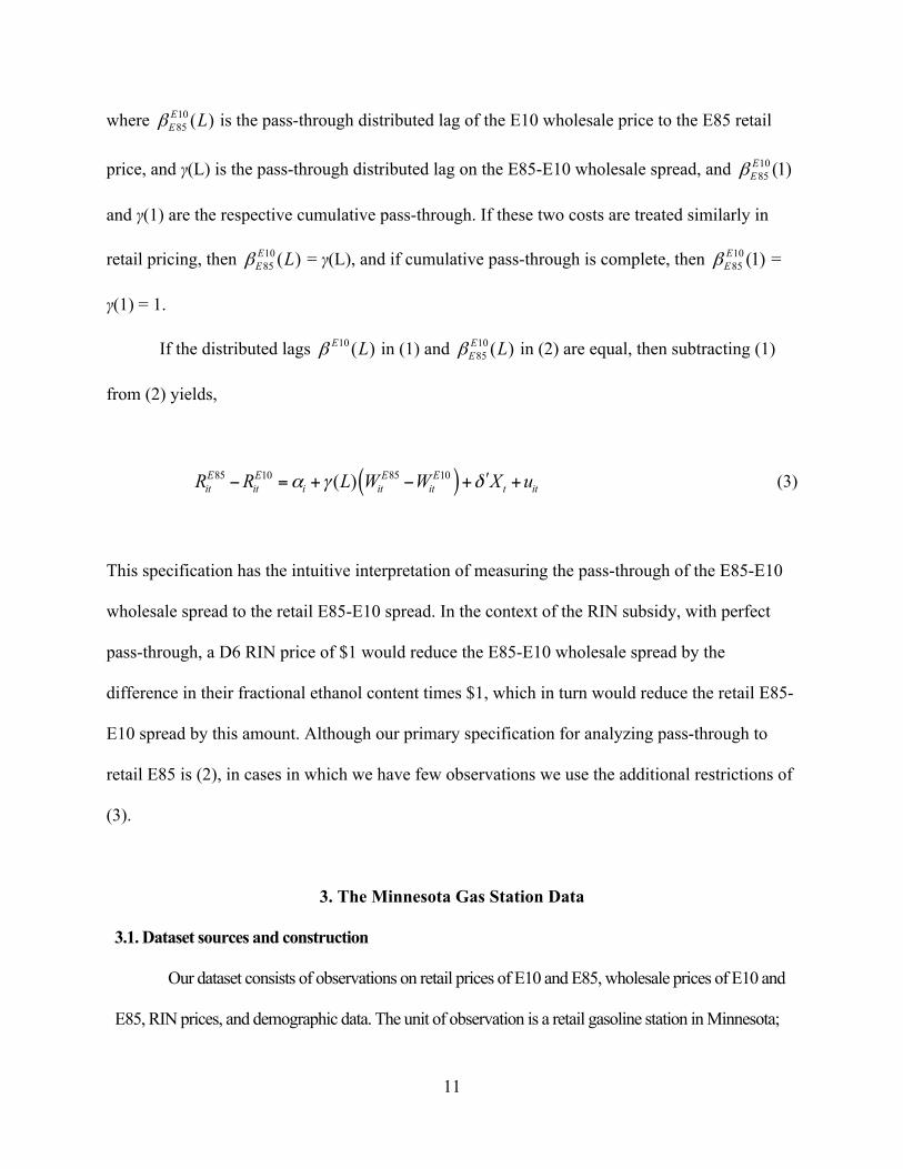
where 1085 ( )EE Lβ is the pass-through distributed lag of the E10 wholesale price to the E85 retail

price, and γ(L) is the pass-through distributed lag on the E85-E10 wholesale spread, and 1085 (1)EEβ

and γ(1) are the respective cumulative pass-through. If these two costs are treated similarly in

retail pricing, then 1085 ( )EE Lβ = γ(L), and if cumulative pass-through is complete, then 10

85 (1)EEβ =

γ(1) = 1.

If the distributed lags 10 ( )E Lβ in (1) and 1085 ( )EE Lβ in (2) are equal, then subtracting (1)

from (2) yields,

( )85 10 85 10( )E E E Eit it i it it t itR R L W W X uα γ δ ʹ− = + − + + (3)

This specification has the intuitive interpretation of measuring the pass-through of the E85-E10

wholesale spread to the retail E85-E10 spread. In the context of the RIN subsidy, with perfect

pass-through, a D6 RIN price of $1 would reduce the E85-E10 wholesale spread by the

difference in their fractional ethanol content times $1, which in turn would reduce the retail E85-

E10 spread by this amount. Although our primary specification for analyzing pass-through to

retail E85 is (2), in cases in which we have few observations we use the additional restrictions of

(3).

3. The Minnesota Gas Station Data

3.1. Dataset sources and construction

Our dataset consists of observations on retail prices of E10 and E85, wholesale prices of E10 and

E85, RIN prices, and demographic data. The unit of observation is a retail gasoline station in Minnesota;

12

all price observations are monthly averages of daily data. The full data span runs from January 2007 to

March 2015.4 All prices are nominal.

We use three subsets of our full dataset.

The MN E10 dataset consists of 231,257 monthly observations on retail and wholesale

prices of E10 at 3,104 Minnesota gas stations. Most of these stations do not sell E85.

The MN E85 dataset consists of 15,970 monthly observations on retail and wholesale

prices of E85 at 398 Minnesota gas stations.

The MN E85-E10 dataset is comprised of stations for which there are data on both E10

and E85 prices, both wholesale and retail. This dataset is constructed by merging the

Minnesota E10 and Minnesota E85 datasets at the station-month level. The dataset is further

restricted by dropping the smallest stations, which we define to be stations that either sell less

than 300 gallons of E85 per month (averaged over months of nonzero volumes), or that report

fewer than 8 months of E85 prices. There are also some stations in the MNDOC dataset that

report selling E85 but are not in the OPIS database, so E10 prices for those stations are not

available; these stations were also dropped. With these exclusions, the MN E85-E10 dataset

consists of 9,983 monthly observations on E85 and E10 prices at 247 stations that sell both

fuels.

These datasets were assembled from multiple sources in four steps.

First, E85 retail price data were obtained from the Minnesota Department of

Commerce (MNDOC), which maintains a monthly survey of retail E85 stations in Minnesota.

Stations report volume-weighted prices obtained from monthly sales quantities and revenues;

4 Though our dataset begins in January 2005, the data on E85 prices are sparse prior to 2007, so the analysis in this paper begins in January 2007.

13

retail prices include all taxes. Earlier vintages of this dataset have been used by Anderson

(2012) and by Liu and Greene (2013) and are further described there. The data used in this

study has two advantages over previous vintages. First, it contains observations during the

period of high RIN prices after January 2013, which permits analyzing RIN price pass-through

to retail prices. Second, our dataset includes the station street address and brand. This permits

matching E85 price data with E10 price data at the station level and also permits accurate

estimation of E85 and E10 wholesale costs at the station level. During 2007-March 2015, 401

stations appear in the MNDOC E85 data.

Second, we obtained from OPIS data on the 3,106 Minnesota gas stations in the OPIS

database. These data consist of station addresses, monthly E10 retail prices, and the OPIS

estimate of the wholesale price paid by each station for E10. The OPIS estimate of the

wholesale price depends on whether the station is branded or unbranded. For branded stations,

OPIS estimates the wholesale price by the rack price for that brand at the closest rack at which

the brand is available. For unbranded stations, the OPIS estimate is the average unbranded

rack price at the closest rack. In both cases, OPIS estimates transportation costs to provide a

delivered E10 wholesale price.

Third, OPIS could not provide an estimated E85 wholesale price at the station level, so

we constructed our own estimate. To do so, we obtained monthly OPIS price data on neat

(pure) petroleum gasoline (E0), on neat ethanol (E100), and on all ethanol blends available for

wholesale purchase at twelve racks in Minnesota, North Dakota, and Iowa, including all seven

racks in Minnesota. The non-Minnesota racks were selected to ensure matching the Minnesota

retailer with the closest rack even if it is outside the state. The wholesale blends for which we

have prices are E10, E60, E65, E70, E75, E80, and E85, however many racks do not have

14

prices on all the higher blends. Discussions with industry indicated that rack E85 contains 83%

ethanol, rack E80 contains 78% ethanol, etc., so that all the E60 – E85 rack blends can be sold

at retail as E85. Our algorithm for estimating the station-level E85 wholesale price is a

modified version of the OPIS algorithm used to estimate the E10 wholesale price. The

modification addresses two key features of E85: first, the ethanol content of retail E85 varies

seasonally so that the blended fuel meets Reid Vapor Pressure standards.5 The seasonal blend

also varies over the period of our sample as environmental standards changed. The seasonal

blend percentage was determined for each month in our sample using American Society for

Testing and Materials (ASTM, multiple) Standard Specifications. For the period of our data,

the blending rate ranges from 74% (sold at the rack as E75) during winter months to 83% (sold

at the rack as E85) during summer months. Given the seasonal blend, we used the following

algorithm for estimating the station wholesale price. For a branded station, we use the

wholesale price at the closest rack selling that brand at the seasonal blend. If a price for that

seasonal blend is not available then we use the next-highest blend. We refer to the wholesale

blend ratio thus determined (e.g. 78% if the wholesale price is for E80) as the month-station

blend ratio. For unbranded stations, we use the same algorithm, except that the station is

assumed to purchase at the OPIS low price for unbranded blends, using the same seasonal

blending and purchasing hierarchy.6

5 The Reid Vapor Pressure (RVP) is a measure of how evaporative a liquid is. Evaporative fuel emissions contribute to ozone so fuel RVP limits vary seasonally. Initially, blending ethanol to E0 increases the RVP, but after approximately 10-15% ethanol, the RVP declines (Andersen et. al. 2010). E10 has a waiver that permits year-round E10 sales but other ethanol blends do not, so the E85 blending ratio must be sufficient to ensure that the blended fuel meets the local and seasonal E0 RVP limit. See Bracmort (2017). 6 As a check, we applied this algorithm (without the higher blend hierarchy) to estimate E10 wholesale prices; the correlation between the station-level E10 wholesale price from our algorithm and the OPIS estimate of the station-level E10 wholesale price over the full dataset is

15

In addition, we used these data to compute a splash-blend wholesale price for retail

E85, which we use in Section 3 as an alternative cost estimate. The splash-blend price is

computed by assuming that the retailer purchases E10 and E100 at the rack, then blends them

in the tanker truck to create the seasonal E85 blend. For example, if the seasonal maximum is

83%, the blend is 81.1% E100 and 18.9% E10. We use the price of E100 with a RIN attached

(during the pre-2013 period, when RIN prices were negligible, we ignore the distinction

between E100 with and without the RIN), and assume that the retailer detaches and sells the

RIN; thus the splash-blend wholesale cost is net of the RIN subsidy. For the subset of stations

that report a retail E85 price, the correlation between our estimated wholesale price and the

splash-blend price is 0.907.

Fourth, we use RIN prices from OPIS and Bloomberg. Using the station-level blending

ratio corresponding to the wholesale price, we computed the net RIN subsidy to station-level

retail E85, compared with E10, that is, the RIN contribution to the E85-E10 retail spread.

3.2. Plots and summary statistics

Figure 2 presents time series plots of quantiles of markups and spreads computed from

the monthly data, January 2007 – March 2015, for the 247 stations in the E85-E10 dataset. Table

I(a) provides summary statistics for the panel datasets (the E10 dataset for E10 and the E85

dataset for E85) and for the E85-E10 dataset.

Several features of the data are noteworthy. First, E85 almost always sells at retail for a

discount relative to E10 on a dollar per gallon basis (Figure 2(c)), consistent with E85 having

0.997. Our wholesale cost estimates are FOB the rack, not delivered. Because distance to the rack is fixed for a given station, however, transportation costs should largely be absorbed by station fixed effects in our panel data regressions.

16

lower energy content than E10. On average, this discount is $0.51, although there is substantial

variation in this discount over time and across stations.

Second, the variation over time and across stations of the markup is substantially greater

for E85 than for E10: the standard deviation of the E85 markup is three times the standard

deviation of the E10 markup.

Third, as is well known, the E10 retail and wholesale prices exhibit seasonality. Table

I(b) reports a test for the significance of monthly dummy variables using the statewide average

time series, in a regression also containing year dummies (Newey-West standard errors). The

markups also have seasonal movements, as do the markup spreads. One driver of the seasonals in

gasoline prices is the shift from winter to summer blendstocks, and the seasonal in E10, which

has high BOB content, is much larger than the seasonal in wholesale E85, which has a smaller

BOB content; it is thus unsurprising that there is seasonal variation in the retail E85-E10 spread.

In principal seasonal fluctuations in E85 demand (perhaps due to cold-start considerations) could

lead to a seasonal in the E85-E10 markup spread, and that seasonal is large ($0.205) but

imprecisely estimated.

Fourth, there are two time periods with multiple missing observations in the E85-E10

dataset, in 2008 and in late 2012. These missing observations relate to lapses in the MNDOC

data collection system, not based on the values of any of the variables, so we treat them as

missing at random.

4. Aggregate Time Series Data and the Volumetric Ethanol Excise Tax Credit

We start by examining the aggregate monthly time series data formed by averaging the

prices in the MN E85-E10 dataset. These data are plotted in Figure 3.

17

Behavior around the expiration of the volumetric ethanol tax credit. Inspection of the

time series data shows an increase in the statewide mean E85 markup in January 2012 (Figures

2b and 2c). The timing of this increase coincides with the end of the federal volumetric ethanol

excise tax credit (VEETC) on December 31, 2011. The VEETC was a subsidy provided for

blending ethanol into motor fuel. During our data sample, this tax credit was $0.51 per gallon of

ethanol through 2009, then $0.45 per gallon through 2011. Bielen, Newell, and Pizer (2016)

undertake an event study of the behavior of prices before and after the VEETC expiration; they

estimate that, at the close of the program, approximately two-thirds of the subsidy was accruing

to ethanol producers, approximately one-third was accruing to blenders, and very little of the

subsidy was accruing to consumers.

Table II reports prices and spreads in the three months before and after the expiration,

from October 2011 to March 2012. The final two columns report changes in the row series from

December 2011 to January 2012, both without seasonal adjustment and seasonally adjusted using

the regression method in Table I(b). The data in Table II are consistent with Bielen, Newell, and

Pizer’s (2016) conclusion that very little of the VEETC subsidy was passed along to the

consumer, at least at the end of the program. In December 2011, the seasonal E85 ethanol

content was 74%, so the full value of the VEETC for E85, minus its value for E10, was (.74-

.1)×$0.45 ≈ 29¢. From December 2011 to January 2012, however, the seasonally adjusted the

retail E10 price rose by 2.2¢ and the retail E85 price rose by 6.6¢, for an increase in the E85-E10

spread of only 4.4¢, consistent with only 4.4¢ of the 29¢ subsidy having been passed on to

consumers.

In these data, the main effect of the VEETC expiration was to decrease the wholesale

price E85 by 25.0¢, and to increase the E85-E10 markup spread by 24.2¢. If the retailer received

18

the tax credit, this is consistent with the retailer’s markup, net of the VEETC, being left roughly

unchanged by the VEETC expiration. If so, then the VEETC subsidy was largely accruing

upstream, to the biorefiner or potentially the farmer. The blender eligible to receive the VEETC

can be the terminal operator or the retailer depending on how the blending is done (splash

blending or rack blending unit) and on ownership or contracting for the delivery truck, see

University of Illinois (2007, p. 157). Even if only some of the retailers received the VEETC, the

mean markup as measured here would change with the VEETC expiration.

The VEETC subsidy was a fixed dollar per gallon subsidy, so the direct effect of the

expiration of the VEETC would be to change the intercept in pass-through regressions relating

wholesale and retail prices.

Pass-through estimates using time series data. Table III reports regressions examining

the dynamic relation between retail and wholesale E85-E10 spreads. The full-sample regressions

(columns (1) and (2)) test for a break in one or more of the regression coefficients (including the

intercept) at an unknown date. The remaining regressions estimate aggregate pass-through rates

for the two samples before and after the VEETC expiration date of Dec. 31, 2011. The pass-

through rates in Table III and in subsequent tables are cumulative over the indicated number of

months.

The results in Table III suggest four main points, which inform the panel data

specifications in the next two sections.

First, consistent with the visual evidence in Figure 3 and the discussion of the VEETC

expiration above, the sup-Wald test for a break using the full sample indicates a break in the

spread regressions, with the break date estimated to be January 2012. In addition to the shift in

the mean E85 markup evident in Figure 3b, the pass-through coefficients change between the

19

two periods: in the 2007-2011 period, pass-through is only 0.42 after one month, but this

increases to 0.72 in the 2012-2015 period. In both periods, pass-through is incomplete, however.

Second, the dynamic regressions indicate that lagged dynamics are significant both

statistically and economically, with cumulative pass-through increasing from contemporaneous

to one month, with a small and statistically insignificant increase after two months. This is

consistent with the time scale of pass-through found in other studies of retail gasoline pricing.

Third, although the fuel prices have large seasonal components, the pass-through

coefficients are insensitive (within a single standard error) to whether seasonals are included or

excluded from the regressions.

Because of the strong institutional and statistical evidence of a break not just in the mean

markup and markup spreads, but also in the pass-through coefficients at the time of expiration of

the VEETC, henceforth we conduct the empirical analysis separately for the two samples before

and after the VEETC expiration date.

5. Panel Data Analysis of Rack-to-Retail Pass-through

We now turn to estimates of wholesale cost pass-through to retail E10 and E85 prices

using the MN E85-E10 panel dataset. We begin with estimates of average pass-through across

stations, that is, the distributed lags β(L) and γ(L) in specifications (1) – (3), estimated by panel

data regression with station fixed effects. We then estimate station-level heterogeneity in pass-

through by estimating separate station-level regressions, where we adjust (deconvolute) the pass-

through estimates for estimation error. Finally, we use panel data regressions with interactions to

examine whether pass-through varies with local competition and with whether the station sells

branded or unbranded gasoline.

20

This section describes and summarizes the empirical results; interpretation of the results

is deferred to Section 6.

5.1. Pass-through regressions.

Table IV presents OLS estimates of pass-through for the two periods, before and after the

VEETC expiration, estimated using the MN E85-E10 dataset. The regressions in Table IV are all

of the form of a retail price or spread regressed on the current value and one lag of one or more

wholesale prices or spreads. The reported coefficients are cumulative pass-through coefficients.

Because all prices are in nominal dollars, a coefficient of 1.00 indicates complete pass-through of

the relevant wholesale cost to the retail price. Consistent with the aggregate time series results,

our base specifications include a contemporaneous term and a single lag. The regressions include

month (seasonal) and station fixed effects. To allow for spatially correlated demand disturbances,

standard errors are clustered at the county level.

The Supplemental Appendix tables report additional specifications and sensitivity checks.

Appendix Table I includes an additional monthly lag, and Appendix Table II excludes the

seasonal dummies. In Appendix Table III, the regressions involving only E10 are estimated

using the full MN E10 dataset and the regressions involving only E85 are estimated using the

MN E85 dataset. Appendix Table IV includes year effects. Appendix Table VI provides

alternative standard errors for Table IV computed using two-way clustering (county and time).

Additionally, some of the appendix tables include regressions estimated over the full sample

period (not split in January 2012).

Four aspects of the results in Table IV and Appendix Tables I-IV are noteworthy.

21

First, for E10, pass-through is complete in both samples (regressions (1)-(2)), and

roughly 80-90% of E10 wholesale costs are passed through in the current month. Cumulative

retail E10 pass-through is estimated to be 1.03 after one month in the pre-2012 sample

(regression (1)) and 0.98 in the post-2012 sample (regression (2)). The large number of station-

level observations result in very small standard errors, even with clustering at the county level,

so these estimates are statistically different from one; however we interpret them as

economically the same as one and consistent with complete pass-through.

Second, pass-through dynamics for E85 are different from those for E10 (regressions (3)-

(6)). Cumulative pass-through is estimated to be large, 0.947 in the pre-2012 period (regression

(3) and 0.953 in the post-2012 period (regression (4)) after one month, but in both periods is

statistically different from one. In addition, pass-through is slower for E85 than for E10, with

current-month pass-through of 74% in the pre-2012 period and 64% in the post-2012 period.

Third, decomposing the wholesale price of E85 into the E10 component and the E85-E10

wholesale spread – that is, estimating specification (2) – reveals that pass-through is very

different for these two components, and moreover that the pass-through coefficients on both

components changed over the two periods. Before 2012, 91.4% (SE = 0.8 pp) of the E10 cost

was passed through to E85 but only 32.3% (SE = 2.1 pp) of the E85-E10 wholesale spread was

passed through. After 2012, there was complete pass-through of E10 costs (one-month

cumulative pass-through of 1.010, SE = .016) to E85, and pass-through of the wholesale spread

rose to 0.525 (SE = .053). In the second period, because the cumulative pass-through of E10

wholesale prices to E85 retail prices is statistically insignificantly different from one, we can

impose this unit coefficient and estimate pass-through using the spread specification (3), which

(not surprisingly) gives a similar pass-through estimate of .501 (SE = .049). These results are

22

robust to removing the seasonal dummies, to including an additional monthly lag, and to

including year effects.

Fourth, these results are robust to including an additional monthly lag (Appendix Table

I), however the pass-through coefficient is smaller if one ignores lagged effects and estimates

only a contemporaneous pass-through regression. The results are also robust to dropping the

seasonals (Appendix Table II). Because specification (1) only involves one fuel, it can be

estimated using the full MN E10 or MN E85 datasets, depending on the fuel, and the results are

robust to using these larger datasets (Appendix Table III); this robustness is suggests that the

merged MN E85-E10 dataset does not introduce sample selection bias. With one exception, the

results are also robust to including year effects in addition to the monthly seasonals (Appendix

Table IV); the sole exception is that the cumulative pass-through coefficient for E10 falls to

0.910 (SE = 0.011) in the second sample (regression (5)). However, when the E10 pass-through

regression is estimated with seasonals and year effects over the full period 2007 – March 2015,

the two-month pass-through coefficient is 1.003 (SE = 0.003, regression (9)). Using two-way

clustering (Cameron et. al. 2011) produces somewhat larger standard errors but does not change

the conclusions substantively (Appendix Table VI). For example, the standard error of the state-

wide cumulative pass-through of 0.347 in the first sample increases from 0.023 to 0.038, and the

standard error of the second-period coefficient of 0.525 increases from 0.053 to 0.068. We rely

on the county-level clustered SEs rather than the two-way clustering for our base specifications

because our panel is heavily unbalanced with time series, a case that appears not to be covered in

the two-way clustering literature.

5.2. Heterogeneity in station-level pass-through

23

We next estimate station-level E85 pass-through coefficients for stations for the two time

periods, where estimates are restricted to stations with at least 18 monthly observations in a

given time period; this restricts the sample to 145 stations in the first period and 94 in the second.

To reduce the number of parameters, the pass-through coefficients are estimated using the spread

– spread specification (3) with no control variables and with the current and a single lagged value

of the wholesale spread, for a total of three coefficients. The station-level cumulative pass-

through coefficients γ(1) are estimated from the station-level time series, so HAC standard errors

are used (Newey-West with 3 lags).

Because of the small number of time series observations per station, the coefficient

estimates have substantial sampling error. We therefore estimate the station-level pass-through

coefficient using a Gaussian-Gaussian decomposition. Specifically, write the OLS estimator of

the cumulative pass-through coefficient for station i as ˆ (1)iγ = ( )ˆ(1) (1) (1)i i iγ γ γ+ − = (1)i ieγ + ,

say, where γi(1) is the unknown station-level pass-through coefficient and ei is OLS estimation

error. The OLS estimation error is plausibly independent of γi(1) and, using the large-sample

approximation, is approximately normally distributed, where var(ei) is estimated by the Newey-

West variance. With the additional assumption that γ (1) is normally distributed across stations,

the Gaussian-Gaussian deconvolution formula can be used to estimate γi(1) as (1)iγ =

( )ˆ(1) | (1)i iE γ γ .7 We use (1)iγ as our estimator of the station-level pass-through coefficient.

7 Specifically, let var(γi(1)) = 2σ and let 2ˆvar( (1) | (1))i i iγ γ τ= . Then (1)iγ =

ˆ ˆ(1) (1 ) (1)i i i iw wγ γ+ − , where wi = ( )2 2 2ˆ ˆ ˆi iτ τ σ+ , where ˆ (1)iγ is the sample average of the

ˆ (1)'i sγ , 2iτ is the Newey-West estimator of 2

iτ , and 2σ is an estimator of 2σ . In unreported results, we modeled γi(1) as a mixture of Gaussian distributions, with no appreciable change in the results. For additional discussion of deconvolution and a recent application to income dynamics see Gu and Koenker (2017).

24

Figure 4 presents a histogram of estimated E85-E10 spread pass-through coefficients

(1)iγ for the two periods. The mean of this distribution is 0.38, with standard deviation 0.19, in

the first period, and is 0.56, with standard deviation 0.21, in the second. These mean values are

close to the coefficients (average treatment effects) of 0.35 and 0.53 estimated in the panel data

estimates in regressions (5) and (6) in Table IV and are consistent with the increase in pass-

through from the first to the second period found in the fixed effect regressions.

5.3. Variation of pass-through with local competition and obligation under the RFS

The histograms in Figure 4 show considerable heterogeneity in station-level pass-

through. We now investigate the extent to which this variation can be explained by the degree of

local competition or by whether the station is affiliated with an obligated party under the RFS.

The motivation for examining the number of local competitors is that, under perfect

competition, pass-through should be one. If there is limited local competition, then gas stations

can exercise local market power, and if so pass-through will in general be different from one.

The variation of pass-through with local competition is estimated using panel data

regressions of the retail E85-E10 spread on distributed lags of the wholesale E85-E10 spread and

the interactions of the wholesale spread with one of two measures of the number of local

competitors. The three measures of local competition are (i) the number of gas stations selling

E85 within 0-3 and 3-10 mile annuli around the station, (ii) the number of gas stations selling

E85 within 0-3 and 3-10 minute driving time from the station, and (iii) whether the station is

located in the Twin Cities (Minneapolis-St. Paul metro area, specifically Hennepin and Ramsey

counties). The Twin Cities has the highest density of E85 stations in our dataset and is

considered to be one of the most mature E85 markets in the nation. As in Table IV, all

25

regressions include station fixed effects, and standard errors are clustered at the county level. We

focus on the second period, which is when there is greater average pass-through.

The results are summarized in Table V. In all cases, more local competition is associated

with higher pass-through. In each specification the interactions are jointly statistically

significant, and the results are robust to including seasonals or not. The effect of local

competitors is greatest if they are nearby, but remains positive and statistically significant if they

are more distant. For example, having an E85 competitor within a 3-minute drive is associated

with a pass-through coefficient that is higher by 0.055 (SE = 0.23, regressions (2)).

The most striking results are when the stations are separated by being in the Twin Cities

or not (regressions (3) and (6)), with stations in the Twin Cities having pass-through coefficients

0.31 greater than stations outside the Twin Cities. In the regression without seasonals, pass-

through for Twin Cities stations is nearly complete, with a coefficient of 0.930 (SE = .003); the

corresponding estimate with seasonals is 0.780 (SE = 0.022).

Because obligated parties need to procure RINs, one possibility is that stations affiliated

with obligated parties act more aggressively to detach the D6 RINs needed by their parent

companies, and as part of that effort pass through more of the RIN value. We can examine this

proposition because the OPIS dataset includes the brand of the gas station, and using public

information we determined whether the station is affiliated with an obligated party. We find,

however, that there is no statistically significant difference in pass-through rates between

obligated-affiliated and non-obligated-affiliated stations (Appendix Figure 1 and Appendix Table

VIII). Another measure of pricing aggressiveness is the difference between the E85 markup and

the E10 markup at a station (the markup spread), with a lower markup spread indicating more

aggressive E85 pricing. In the high-RIN period starting January 2013, this markup spread was

26

essentially the same in obligated-affiliated and non-obligated-affiliated stations, being lower in

obligated-affiliated stations by only $0.037 (SE = 0.038). These results find no evidence of

difference in pricing behavior between stations affiliated with obligated parties, and those not.

The lack of effect of obligation on pricing behavior is consistent with stations facing the

same profit maximizing incentives. If a station has local E85 market power, it is in its financial

interest to price accordingly, but if it is in a competitive local E85 market as in the Twin Cities, it

will price competitively and pass through its marginal cost. This incentive for station-level profit

maximization is the same whether or not the station is affiliated with an obligated party.

5.4. Effect of entry

The regressions in Table V establish that pass-through is greater if there are more local

competitors in the E85 market, but because the decision to sell E85 is endogenous, those

regressions do not establish a formal causal link. Our dataset allows us to examine the effect of

entry of a local competitor, however, so here we exploit these entry events to estimate the effect

of competition on markups and pass-through. We define an E85 entry event as an increase in the

number of E85 stations within a circle of a given radius, compared to the previous month. In

most cases, this entry event corresponds to a new station entering the MN DOC database. In

some cases, stations appear to sell E85 either seasonally (not offering E85 in the winter) or have

an extended period of E85 sales, then an extended period of no sales, then a period of sales.8 We

consider separately the effect of entry on mean markups, and the effect of entry on pass-through.

8 Because stations are required to report prices and volumes if they received state funding for their E85 investment, it is plausible that most of these periods of no report sales actually represent zero sales rather than simply a lapse in reporting. To the extent that some of our identified entry events are in fact just periods of random data reporting lapses, our estimated effects of entry would be attenuated because of classical errors-in-variables bias.

27

Table VIA summarizes the dynamic effect of entry on markups, estimated for entry

defined over circles of radii 3, 4, and 5 miles. The dependent variable is the E85 markup; the

regressors are dummy variables indicating the months prior to entry (t+1, etc.), the month of

entry, and months after entry (t-1, etc.). The change in the markup reported in the table is the

difference between the average coefficient for the four months after the entry, minus the average

for the four months before entry. The regressions have station fixed effects, so the coefficients

have a differences-in-differences interpretation (before vs. after, stations with entry at a given

date vs. those without).

The estimates in Table VIA are consistent with substantial and statistically significant

effects of entry on average markups: in the first period, an entry within four miles is estimated to

decrease the markup by -13.5¢ (SE = 2.5). The point estimates of the effect of entry are similar

in the two periods, although there are few entry events in the second period so the standard errors

are large. (Results for a 3-mile radius in the second period are omitted because there are only 4

of these entry events, and there are only 12 within a 4 mile radius.) The dynamics of the markup

response is similar across all estimates in Table VIA, with the markup beginning to decline in the

month prior to entry and the largest decline occurring in the month of entry and the month after

entry. The anticipatory decline is consistent with the ability of a retail operator to observe the

construction associated with an existing local E10 station adding the ability to sell E85 by

installing a blender pump or, possibly, upgrading its tanks.

Table VIB reports estimates of changes in pass-through coefficients, estimated in fixed

effects regressions of the retail E85-E10 spread on the current and first lagged values of the

wholesale E85-E10 spread and that spread interacted with two indicators, one denoting the

twelve months up before the entry event and one denoting the twelve months commencing with

28

the entry event. The Table VIB estimates are a triple-difference estimate of the change in E85

pass-through associated with an entry event. In both samples, the estimates for entries within 4

and within 5 miles are positive, and the magnitude of the coefficients is comparable to Table V.

Because of the few entry events, however, the estimation error in this triple difference estimate

of regression coefficients is large and none of these estimated differences in E85-E10 pass-

through are statistically significant. Still, we take the results in Table VIB as weakly supportive

of interpreting the more precise results in Table V as evidence that local competition increases

pass-through.

5.5. Alternative purchasing assumptions

The analysis so far assumes that retailers purchase blended fuel at the rack. Under this

assumption, the blended fuel already has the RIN detached so the retailer never touches a RIN.

There are, however, two other purchasing and blending strategies used by some retailers. Under

the first, examined in this subsection, a retailer purchases E10 and pure ethanol with a RIN at the

rack (E100w) and “splash blends” the two fuels in the tanker truck. Under the second, examined

in the next section, the retailer purchases fuel upstream of the rack and typically pays a price

pegged to the bulk exchange at the origin of the pipeline and from the biorefiner. Both strategies

change the RIN ownership chain, so the retailer ends up owning the RIN. As a result, both

strategies have expression for the wholesale marginal cost that differ from each other and from

the marginal cost for purchasers of blended fuels at the rack.9

9 Detaching and selling a RIN entails administrative overhead, including registering with the EPA to be part of the RIN chain of custody. Because of these fixed costs, these strategies tend to be used primarily by larger retail outlets.

29

For splash blending of fuels purchased at the rack, if the seasonal blend ratio is ω, then

the retailer blends ( .1) / .9ω ω= − gallons of E100w with (1 )ω− gallons of E10, and detaches

and owns ω D6 RINs. The retailer’s wet fuel cost is 85,E SBitW = 100 10(1 )E w E

it itW Wω ω+ − . The full

marginal wholesale cost for a splash blender (SB) subtracts off the value of the RIN detached

and sold by the retailer, 85, 6E SB Dit tW Pω− , where 6D

tP is the price of the D6 RIN. Because E10 is

sold at the rack without a RIN, the E85-E10 wholesale spread is ( )85, 10 6E SB E Dit it tW W Pω− − , where

the first term is the wet fuel spread between splash blended E85 and E10, and the second term is

the value of the RIN sold by the retailer. With perfect competition, this marginal cost would be

passed through to price, but under imperfect competition there could be incomplete pass-through

and moreover the pass-through rates for the RIN price and the wet fuel spreads could be

different. This leads to the pass-through regression for splash blending:

( )85 10 , 85, 10 , 85,( ) ( )E E SB fuel E SB E SB RIN E SBit it i it it it t itR R L W W L RIN X uα γ γ δ ʹ− = + − + + + , (4)

where 85,E SBitRIN = 6D

tPω− and ω is determined by the seasonal E85 blending ratio. Under

perfect competition, the cumulative pass-through coefficients on the wet fuel and RIN

components are both one: , (1)SB fuelγ = , (1)SB RINγ = 1.

Table VII presents estimates of specification (4) for the full state, the Twin Cities, and

outside the Twin Cities, where the rack price of E100w is used to compute the splash-blend

wholesale price for E85. Statewide, the splash-blending pass-through rate for the wholesale

splash-blending E85-E10 spread is .574 (SE = .064), the pass-through for the RIN component is

less (0.393), and the restriction that the pass-through rates equal each other is rejected. In the

30

Twin Cities, both the wet fuel and RIN pass-through rates are larger, 0.864 (SE = 0.044) and

0.792 (SE = 0.046), respectively, and are not statistically different from each other. Results

without seasonals (Appendix Table VII) are very close to those with seasonals.

The splash-blending results in Table VII are similar to the results in Tables IV and V,

which assume purchase of blended fuels: the statewide blended fuel pass-through coefficient is

0.525, for splash blending it is 0.574; in the Twin Cities, the blended fuel pass-through

coefficient is 0.930, in the Twin Cities the splash-blended coefficient is 0.864. This result is not

surprising: any retailer who has the administrative infrastructure in place to sell RINs can seize

the opportunity to arbitrage at the rack between purchasing blended fuel or splash-blending and

retaining the RIN.

Retailers have other blending options too. Large chains have the ability to purchase fuel

upstream of the rack and pay the terminal owner a service charge for handling the fuel; whether

the fuel is delivered blended or splash blended, the retailer retains the RIN and pays an upstream,

not rack, price for the fuel. If the upstream price is a bulk exchange price (plus transportation

charges), then rack pricing is bypassed altogether, and the wholesale price and RIN charge is that

considered in the next section (equations (5) and (6) below). These strategies are different ways

for the retailer to obtain blended fuel and thus to arbitrage the rack price. Our findings are

consistent with retail pass-through rates not depending on the method used to obtain the blended

fuel, however we cannot test that directly because we do not know the method used at the station

level.10

10 Another option for blending higher blends available to some retailers is purchasing E85 directly from a biorefinery, which splash blends its ethanol with natural gasoline. In this arrangement, the biorefinery retains and sells the RIN, so it is competing directly with blended fuel at the rack. To the extent that the biorefinery sets its blended fuel price as a discount off the blended fuel rack price (which is plausible, since the retailer can instead buy the blended fuel

31

6. Discussion and Implications for RIN Pass-Through

These empirical results in Sections 4 and 5 lead us to four main conclusions.

First, the complete pass-through of E10 after one month is consistent with the Minnesota

E10 retail market being highly competitive. This conclusion is consistent with results in the

existing literature, which finds complete pass-through in the U.S. retail E10 market, with pass-

through dynamics lasting 4-8 weeks.

Second, these results are consistent with imperfect competition in the retail E85 market,

with stations having local market power. When there are more local competitors, that market

power is reduced, and there is greater pass-through. The magnitude of this effect is substantial:

according to the estimates in Table V regression (2), a station with 2 competitors within a 3

minute drive and with 7 competitors within 3-10 minutes (both are the 90th percentile of these

distributions) will pass through 22 percentage points more of the E85-E10 wholesale spread to its

E85 retail customers than a station with no competitors within a ten minute drive.

Third, the weight of the evidence – the time series evidence in Table III, the panel data

estimates of specification (2), and the histograms in Figure 4 – points to a change in the market

structure around January 2012. Although we have highlighted the expiration of the VEETC as

the event separating the two periods, the increasing pass-through coefficient could be unrelated

to the VEETC expiration and could simply reflect maturing of the industry and an increase in

from the terminal), this strategy would be captured by the specifications in Tables IV and V, and the biorefinery discount would be captured in the station fixed effect. We are not able to study this pricing approach because data on pure ethanol prices at the refinery gate are not available in Minnesota (although they are in Iowa), nor is the price of natural gasoline. This strategy has the disadvantage of being illegal because the natural gasoline blend does not satisfy other environmental regulations for E85.

32

consumer awareness of where E85 stations are, facilitated by state highway signage indicating

E85 stations (Minnesota Department of Transportation (2006)). Alternatively, this change in

pass-through could instead be associated with changing pricing dynamics in the high-RIN period

starting in January 2013. Despite this evolution towards increasing pass-through, our estimates

suggest that, on average, pass-through of the E85-E10 wholesale spread to E85 retail prices

remained partial, with our preferred statewide pass-through estimate being .525 (SE = .053,

Table IV(6)).

Implications for RIN pass-through. Because the net effect of a movement in RIN prices

on E10 prices is negligible, both in theory and based on empirical evidence (Knittel, Meiselman,

and Stock (2017)), the RIN subsidy to E85 operates through the E85-E10 wholesale spread. The

partial pass-through of the E85-E10 spread to E85 prices suggests that any RIN price subsidy

passed through at the rack in the form of lower prices for blended fuels, passes through only

partially to the end retail customer. Our preferred overall estimate of 0.525 pass-through

indicates that only half the RIN subsidy at the rack is passed through to lower retail E85 prices.

We examine RIN pass-through by two additional sets of regressions, in this case with

RIN prices and upstream bulk wholesale cost spreads as regressors. These regressions examine

the extent to which the subsidy for blending ethanol at the rack is passed on to posted rack

prices, and then downstream to retail prices. The subsidy for blending ethanol into E10 is 0.1

times the D6 RIN price, and the subsidy for blending ethanol into E85 is the seasonal blend rate

times the D6 RIN price. As before, we focus on the E85-E10 spread, which controls for

fluctuations in oil prices and the fuels markets, and the net ethanol blending subsidy 85 10E EtRIN −

is the difference between the E85 and E10 blending subsidies. We estimate bulk wholesale costs

using the Gulf CBOB price and the Chicago Mercantile Exchange ethanol price (daily data from

33

the Energy Information Administration and Bloomberg, respectively, aggregated to monthly),

using the E10 and the seasonal E85 blending ratios. Our regressions have the form,

( )85 10 85 10 85 10( ) ( )E E WB E E W E Eit it i t t t t itW W L B B L RIN X uα γ θ δ− ʹ− = + − + + + (5)

( )85 10 85 10 85 10( ) ( )E E RB E E R E Eit it i it it t t itR R L B B L RIN X uα γ θ δ− ʹ− = + − + + + (6)

where 85EtB and 10E

tB are the bulk wholesale costs of E85 and E10.

A key thing to note is that 10EtB is a price above the rack, so that the ethanol component

includes a RIN; the RIN is detached upon blending at the rack. If there is complete pass-through

at the rack, then (1)WBγ = (1)Wθ = 1. If there is complete pass-through all the way down the

supply chain, from bulk wholesale to retail, then (1)RBγ = (1)Rθ = 1. If the cost of the wet fuels

is passed on at the rack, but the RIN subsidy is only partially passed on, then (1)WBγ = 1 but

(1)Wθ < 1. Because the blended fuel does not have a RIN attached, there is no reason to think

that the RIN price would affect the price at retail other than through the price of the blended fuel.

In the notation of equation (3), the cumulative pass-through in the E85-E10 spread is γ(1) from

rack (blended) to retail. Thus, one would expect long-run RIN pass-through at retail to satisfy

(1)Rθ = (1) (1)Wγ θ . Said differently, a fraction (1)Wθ of the RIN value is passed along at the

rack, and of that, a fraction γ(1) is passed along at the pump; thus the consumer sees (1) (1)Wγ θ

of the RIN value in the retail spread between E85 and E10.

Equation (6) has an additional interpretation. As discussed in Section 5.5, some retail

chains occasionally purchase petroleum blendstock (E0) and E100w above the rack, then blend it

34

at the rack, paying a user fee to the terminal operator. In this case, the retailer does not pay the

rack price for fuel and retains and sells the RIN. If the price paid for the fuel above the rack is

pegged to the bulk exchange prices, then Equation (6) is the relevant pass-through equation for

retail chains that purchase fuel above the rack.

Table VIII presents results of estimation of regressions (5) and (6). The table separates

the Twin Cities from the rest of Minnesota because of the large differences in pass-through and

competition found between the two areas in Table V; pooled results for the full state are

presented in the final two columns. Results are only for the second period, which is the only

relevant period with nontrivial D6 RIN prices.

The results in Table VIII are consistent with complete pass-through at the rack, with

cumulative pass-through coefficients insignificantly different from 1 and insignificantly different

from each other; these coefficients are imprecisely estimated because there is a single Twin

Cities rack in our data and we use time series regression with HAC standard errors. In the Twin

Cities, the RIN pass-through to retail is estimated to be 0.803 (SE = 0.049), consistent with the

pass-through of blended rack to retail of 0.78 (Table V(6)) and complete rack pass-through.

These pass-through rates are estimated to even higher without the seasonals (0.988, SE = 0.080,

in Table VIII(3)). Thus, the results for Minneapolis are consistent with complete pass-through at

the rack, complete or nearly complete pass-through at retail, and with the retail consumer seeing

the full, or nearly full, RIN subsidy.

In contrast, outside the Twin Cities, pass-through is estimated to be less both at the rack

and at retail: with seasonals, ˆ (1)Wθ = 0.743 and ˆ (1)Rθ = 0.311. This latter estimate is consistent

with the estimate of ˆ (1)Rθ = ˆˆ(1) (1)Wγ θ = 0.466×0.743 = 0.346. Outside the Twin Cities, in our

sample approximately three-fourths of the RIN value is passed on at the rack, and of that just

35

under one-half is passed on at retail, so the consumer sees roughly one-third of the RIN value in

the E85-E10 spread.11

The estimates of pass-through of RIN prices to the E85-E10 spread found here are greater

than found in Knittel, Meiselman, and Stock (2017). Using weekly data on national average E85

prices, they estimated cumulative RIN pass-through to the E85-E10 retail spread of 0.23 after six

weeks in their distributed lag specification that is closest to the distributed lag specifications used

here. Their results used national average E85 prices, which includes markets that are less mature

than in Minnesota. Our results indicate lower pass-through in areas of lower competition, and we

suspect this, or issues of data quality in the national time series, is the most likely reason for the

national RIN pass-through being lower than the Minnesota RIN pass-through estimated here.

These estimates of RIN pass-through are also consistent with those in Lade and Bushnell

(2016). As they point out, their data sample heavily represents urban centers (Minneapolis, Des

Moines, and Chicago) where there is strong competition in E85. In contrast, our dataset contains

many rural stations that have few if any local competitors. The results for our data, restricted to

the Twin Cities, are consistent with their finding of complete pass-through.

Because we only have data for Minnesota, we cannot speak to pass-through rates in other

states. That said, in the Twin Cities, where pass-through is essentially complete and where there

is a competitive market, E85 sales per capita are roughly twice those outside the Twin Cities,

where station density is lower and pass-through is less. Outside the Midwest, E85 station density

is very low, and our results suggest that one would find low pass-through and low E85 sales in

such cases.

11 These estimated pass-through findings at the rack are consistent with preliminary estimates in Pouliot, Smith, and Stock (2017).

36

Broader implications. The mechanism whereby the RFS incentivizes consumers to use

more ethanol is the RIN subsidy. For this subsidy to be effective, it must reach the consumer in

the form of lower prices for higher ethanol blends. The evidence presented here suggests that this

occurs incompletely. Overall in our data, roughly half the rack discount of E85 off E10 –

including that part of the discount due to the RIN subsidy – is passed along to the consumer,

while half of the RIN subsidy that is passed through at the rack accrues to the station operator.

Our results also suggest that greater E85-on-E85 competition increases RIN pass-through. The

most obvious form for this increased competition is through increased station density, but other

methods on which we do not have data, such as improved signage or Web posting of E85 prices

could also matter. A specific implication of this analysis is that programs such as the $210

million USDA Biofuels Infrastructure Partnership in 2015 could substantially increase the

fraction of the RIN subsidy passed along to the consumer and thus increase the efficiency and

effectiveness of the RFS program. To do so, such subsidies should be targeted to promote E85 on

E85 retail competition through increasing station density, otherwise they will simply help the

participating retailer establish a chain of local E85 monopolies.

37

References

American Society for Testing and Materials (multiple): Standard Specifications for Ethanol Fuel

Blends for Flexibile-Fuel Automotive Spark-Ignition Engines, ASTM International:

D5798-06.21306, D5798-07.16159, D5798-09.9170, D5798-09a.4376, D5798-

09B.39298, D5798-10.33882, D5798-10a.28876, D5798-11.22603, D5798-12.17402,

D5798-13.10747, D5798-13a.3129, D5798-14.32148, D5798-99.31268, D5798-

99R04.26202, and D5798.17164.

Andersen, V.F., J.E. Anderson, T.J. Wallington, S.A. Mueller, and O.J. Nielsen. 2010. “Vapor

Pressures of Alcohol-Gasoline Blends.” Energy Fuels 24, 3647-3654.

Anderson, Soren. 2012. “The Demand for Ethanol as a Gasoline Substitute.” Journal of

Environmental Economics and Management 63(2), 1512-168.

Bachmeier, Lance J., and James M. Griffin. 2003. “ New evidence on asymmetric gasoline price

responses. ” Review of Economics and Statistics 85 (3): 772-776.

Bielen, David A., Richard G. Newell, and William A. Pizer. 2016. “Who Did the Ethanol Tax

Credit Benefit? An Event Analysis of Subsidy Incidence.” NBER Working Paper No.

w21968.

Borenstein, Severin, A. Colin Cameron, and Richard Gilbert. 1997. “Do gasoline prices respond

asymmetrically to crude oil price changes? ” The Quarterly Journal of Economics 112

(1): 305-339.

Borenstein, Severin, and Andrea Shepard. 2002. “Sticky prices, inventories, and market power in

wholesale gasoline markets.” RAND Journal of Economics 33 (1): 116–139.

Bracmort, Kelsi. 2017. “Reid Vapor Pressure Requirements for Ethanol,” Congressional

Research Service, May 18, 2017.

Burkhardt, Jesse. 2016. “Incomplete regulation in an imperfectly competitive market: the impact

of the renewable fuel standard on U.S. oil refineries. ” manuscript, School of Forestry and

Environmental Studies, Yale University.

Burkholder, Dallas. 2015. “A Preliminary Assessment of RIN Market Dynamics, RIN Prices,

and their Effects.” http://www.regulations.gov/#!documentDetail;D=EPA-HQ-OAR-

2015-0111-0062.

Cameron, A. Colin, Jonah B. Gelbach, and Douglas L. Miller. 2011. “Robust Inference with

38

Multiway Clustering.” Journal of Business & Economic Statistics 29(2): 238-249.

Coglianese, John, Lucas W. Davis, Lutz Kilian, and James H. Stock. 2016. “Anticipation, Tax

Avoidance, and the Price Elasticity of Gasoline Demand.” Journal of Applied

Econometrics 32(1): 1-15.

Corts, K. 2010. “Building Out Alternative Fuel Retail Infrastructure: Government Fleet

Spillovers in E85.” Journal of Environmental Economics and Management 59(3), 219-

234.

Gu, Jiaying and Roger Koenker. 2017. “Unobserved Heterogeneity in Income Dynamics: An

Empirical Bayes Perspective.” Journal of Business & Economic Statistics 35(1): 1-16.

Irwin, Scott. 2013a. “What’s behind the plunge in RIN prices? ” farmdoc daily (3):193.

Department of Agricultural and Consumer Economics, University of Illinois. October 10.

Irwin, Scott. 2013b. “More on ethanol RINs pricing. ” farmdoc daily (3):208. Department of

Agricultural and Consumer Economics, University of Illinois. October 31.

Irwin, Scott. 2014. “Rolling back the write down of the renewable mandate for 2014: The RINs

market rings the bell again. farmdoc daily (4):148. Department of Agricultural and

Consumer Economics, University of Illinois. August 8.

Irwin, Scott. 2015. “Implications of changing the biodiesel tax credit from a blender to a

producer credit”. farmdoc daily (5):142. Department of Agricultural and Consumer

Economics, University of Illinois. August 8.

Knittel, Christopher R. and Aaron Smith. 2015. “Ethanol production and gasoline prices: A

spurious correlation.” The Energy Journal 36 (1): 73-113.

Knittel, Christopher R., Ben S. Meiselman, and James H. Stock. 2017. “The pass-through of RIN

prices to wholesale and retail fuels under the Renewable Fuel Standard.” Journal of the

Association of Environmental and Resource Economists 4(4): 1081-1119.

Lade, Gabriel E. and James Bushnell. 2016. “Fuel Subsidy Pass-through and Market Structure:

Evidence from the Renewable Fuel Standard.” Working Paper 16-WP 570, CARD, Iowa

State University, December 2016.

Lade, Gabriel E., C.-Y. Cynthia Lin, and Aaron Smith. 2015. “The effect of policy uncertainty

on market-based regulations: Evidence from the Renewable Fuel Standard.” manuscript,

Department of Agricultural and Resource Economics, University of California, Davis.

Lewis, Matthew S. 2011. “Asymmetric price adjustment and consumer search: An examination

39

of the retail gasoline market.” Journal of Economics & Management Strategy 20 (2):

409–449.

Liu, Changzheng and David Greene. 2013. “Modeling the Demand for E85 in the United States,”

manuscript, at http://info.ornl.gov/sites/publications/files/Pub45616.pdf.

Liao, Kenneth and Sébastien Pouliot. 2015. “Econometric Analysis of Motorists’ Preference for

Ethanol in Motor Fuels.” manuscript, Iowa State University, 2015. Minnesota

Department of Transportation. 2006. Minnesota E85 Highway Signage Program.

Owyang, Michael, and E. Katarina Vermann. 2014. “Rockets and feathers: Why don’t gasoline

prices always move in sync with oil prices?” The Regional Economist.

https://www.stlouisfed.org/Publications/Regional-Economist/October-2014/Rockets-and-

Feathers-Why-Dont-Gasoline-Prices-Always-Move-in-Sync-with-Oil-Prices.

Pouliot, Sébastien, and Bruce Babcock. 2017. “Feasibility of Meeting Increased Biofuel

Mandates with E85.” Energy Policy 101: 194-200.

Pouliot, Sébastien, Aaron Smith, and James H. Stock. 2017. “RIN Pass-Through to Prices of E10

and Higher Ethanol Blends at the Terminal Rack.” manuscript.

Salvo, Alberto, and Cristian Huse. 2013. “Build it, but will they come? Evidence from consumer

choice between gasoline and sugarcane ethanol.” Journal of Environmental Economics

and Management 66(2), 251-279.

Stolper, Samuel. 2016. “Who bears the burden of energy taxes? The critical role of pass-

through.” manuscript, Harvard Kennedy School.

University of Illinois. 2007. “Corn-Based Ethanol in Illinois and the U.S.: A Report from the

Department of Agricultural and Consumer Economics,” University of Illinois.

40

Figure 1. RIN price determination in terms of market fundamentals

Source: Knittel, Meiselman, and Stock (2017).

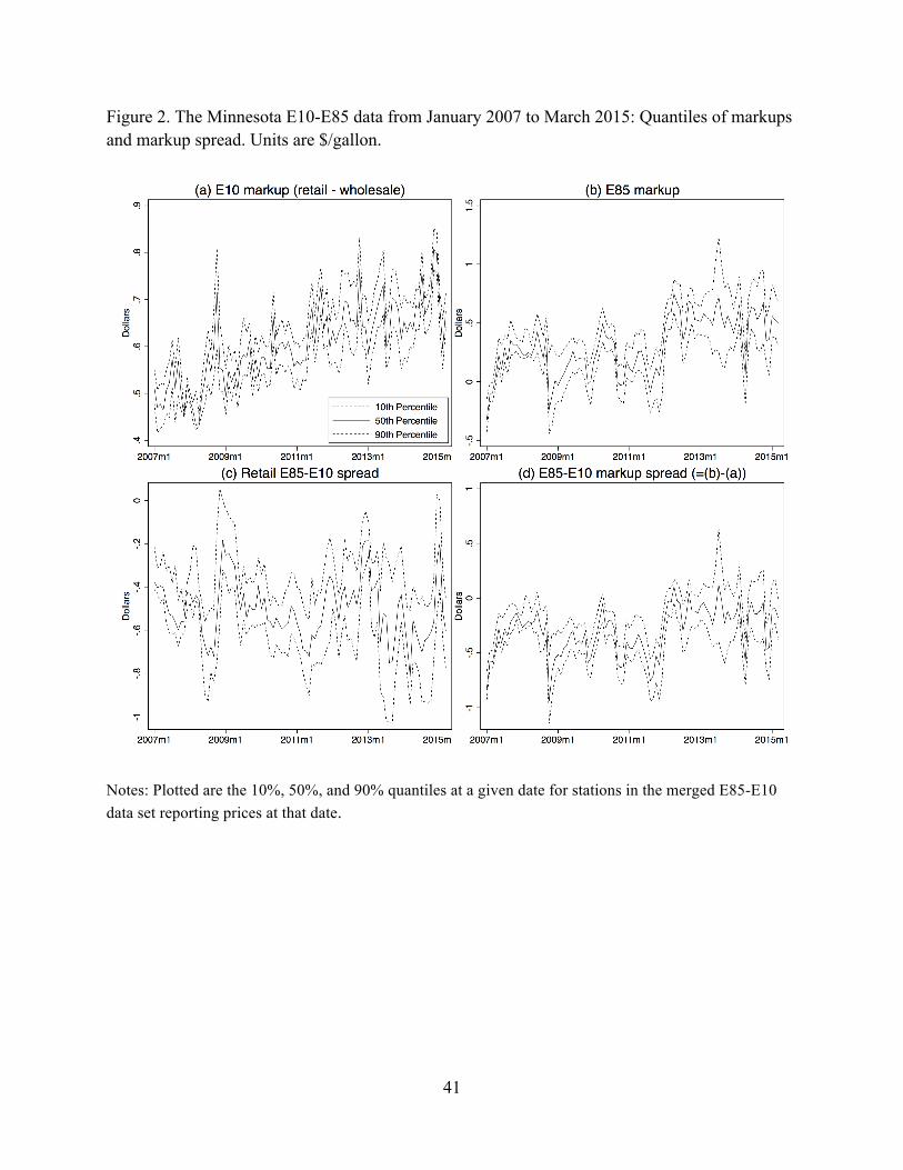
41

Figure 2. The Minnesota E10-E85 data from January 2007 to March 2015: Quantiles of markups and markup spread. Units are $/gallon.

Notes: Plotted are the 10%, 50%, and 90% quantiles at a given date for stations in the merged E85-E10 data set reporting prices at that date.

42

Figure 3. E10 and E85 prices and spreads: statewide average time series constructed from the E85-E10 dataset. Solid-retail; dashed-wholesale. Vertical line denotes January 2012.

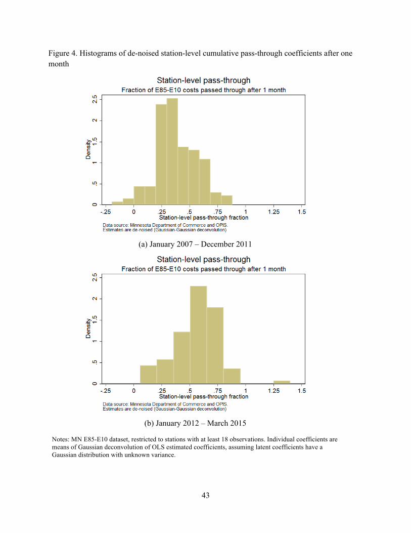
43

Figure 4. Histograms of de-noised station-level cumulative pass-through coefficients after one month

(a) January 2007 – December 2011

(b) January 2012 – March 2015

Notes: MN E85-E10 dataset, restricted to stations with at least 18 observations. Individual coefficients are means of Gaussian deconvolution of OLS estimated coefficients, assuming latent coefficients have a Gaussian distribution with unknown variance.

44

Table I. Summary statistics

(a) Panel datasets

mean Std. dev.

min max

MN E10 dataset: No. stations = 3,104, N = 231,257 retail E10 3.07 0.56 1.76 3.94 wholesale E10 2.45 0.53 1.21 3.34 E10 markup = retail E10 – wholesale E10 0.62 0.10 0.43 0.87 MN E85 dataset: No. stations = 398, N = 15,970

retail E85 2.59 0.50 1.47 3.48 wholesale E85 2.29 0.47 1.11 3.35 E85 markup = retail E85 – wholesale E85 0.30 0.28 -0.32 1.02 MN E85 dataset: No. stations = 247, N = 9,983

E85-E10 retail spread = retail E85 – retail E10 -0.51 0.22 -1.03 0.01 E85-E10 wholesale spread = wholesale E85 – wholesale E10 -0.21 0.28 -0.85 0.42 E85-E10 markup spread = E85 markup – E10 markup = E85-E10 retail spread – E85-E10 wholesale spread

-0.30 0.28 -0.96 0.37

(b) Seasonality in time series data: January 2007 – March 2015 F-statistic p-value seasonal range ($/gal) retail E10 3.64 0.000 0.629 wholesale E10 3.09 0.002 0.619 E10 markup 7.95 0.000 0.091 retail E85 1.85 0.060 0.422 wholesale E85 1.55 0.130 0.285 E85 markup 2.92 0.003 0.205 E85-E10 retail spread 3.59 0.000 0.263 E85-E10 wholesale spread 2.53 0.009 0.367 E85-E10 markup spread 1.55 0.129 0.205

Notes: The E85-E10 dataset consists of observations on stations which (i) have at least eight months in which retail and wholesale prices of E10 and E85 are all observed, and (ii) have monthly E85 sales averaging least 300 gallons. The test for seasonality in part (b) is computed using the monthly time series equaling the statewide average by month, averaged over observations in the E85-E10 dataset. This series is regressed on eleven monthly dummy variables and a full set of year dummies; the reported F-statistic tests the hypothesis that the coefficients on the monthly dummies are zero (Newey-West variance, 6 lags), and the seasonal range is the range of the predicted seasonals in this regression. All units are dollars per gallon.

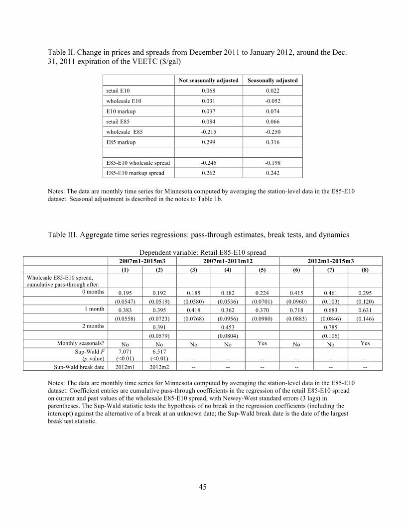
45

Table II. Change in prices and spreads from December 2011 to January 2012, around the Dec. 31, 2011 expiration of the VEETC ($/gal)

Not seasonally adjusted Seasonally adjusted

retail E10 0.068 0.022

wholesale E10 0.031 -0.052

E10 markup 0.037 0.074

retail E85 0.084 0.066

wholesale E85 -0.215 -0.250

E85 markup 0.299 0.316

E85-E10 wholesale spread -0.246 -0.198

E85-E10 markup spread 0.262 0.242

Notes: The data are monthly time series for Minnesota computed by averaging the station-level data in the E85-E10 dataset. Seasonal adjustment is described in the notes to Table 1b. Table III. Aggregate time series regressions: pass-through estimates, break tests, and dynamics

Dependent variable: Retail E85-E10 spread

2007m1-2015m3 2007m1-2011m12 2012m1-2015m3 (1) (2) (3) (4) (5) (6) (7) (8) Wholesale E85-E10 spread, cumulative pass-through after:

0 months 0.195 0.192 0.185 0.182 0.224 0.415 0.461 0.295 (0.0547) (0.0519) (0.0580) (0.0536) (0.0701) (0.0960) (0.103) (0.120)

1 month 0.383 0.395 0.418 0.362 0.370 0.718 0.683 0.631 (0.0558) (0.0723) (0.0768) (0.0956) (0.0980) (0.0883) (0.0846) (0.146)

2 months 0.391 0.453 0.785 (0.0579) (0.0804) (0.106)

Monthly seasonals? No No No No Yes No No Yes Sup-Wald F

(p-value) 7.071

(<0.01) 6.517

(<0.01) -- -- -- -- -- -- Sup-Wald break date 2012m1 2012m2 -- -- -- -- -- --

Notes: The data are monthly time series for Minnesota computed by averaging the station-level data in the E85-E10 dataset. Coefficient entries are cumulative pass-through coefficients in the regression of the retail E85-E10 spread on current and past values of the wholesale E85-E10 spread, with Newey-West standard errors (3 lags) in parentheses. The Sup-Wald statistic tests the hypothesis of no break in the regression coefficients (including the intercept) against the alternative of a break at an unknown date; the Sup-Wald break date is the date of the largest break test statistic.

46

Table IV. Station-level cumulative pass-through regressions using the E85-E10 dataset

Dependent variable Retail E10 Retail E85 Retail E85-

E10 Spread (1) (2) (3) (4) (5) (6) (7)

Dates 2007m1-2011m12

2012m1-2015m3

2007m1-2011m12

2012m1-2015m3

2007m1-2011m12

2012m1-2015m3

2012m1-2015m3

Wholesale E10, lag 0

0.892 0.831 0.739 0.712 (0.00861) (0.00807) (0.0274) (0.0327)

Wholesale E10, lag 1

1.031 0.979 0.916 1.010 (0.00225) (0.00433) (0.00782) (0.0155)

Wholesale E85, lag 0

0.694 0.644 (0.0208) (0.0274)

Wholesale E85, lag 1

0.947 0.953 (0.00872) (0.0203)

Wholesale E85-E10 spread, lag 0

0.172 0.230 0.160 (0.0155) (0.0360) (0.0311)

Wholesale E85-E10 spread, lag 1

0.347 0.525 0.501 (0.0229) (0.0529) (0.0491)

N 5,521 4,288 5,424 4,277 5,424 4,277 4,277 Number of

stations 215 175 215 175 215 175 175

Monthly seasonals? Yes Yes Yes Yes Yes Yes Yes

Notes: Entries are pass-through coefficients in the regression of the retail price or the retail price spread (regression (6), panel B) on the current value, or current and one lagged value, of the indicated wholesale price or price spread. For regressions including the lag, the reported coefficient is the cumulative pass-through (cumulative sum of coefficients on lagged values). Panel A, regression (5) includes year fixed effects to allow for the expiration of the VEETC; none of the other regressions include year fixed effects. Standard errors are clustered at the county level and are given in parentheses. All regressions include station-level fixed effects.

47

Table V. Variation of cumulative pass-through with local competition

Dependent variable: retail E85-E10 spread (1) (2) (3) (4) (5) (6)

Dates 2012m1-2015m3

2012m1-2015m3

2012m1-2015m3

2012m1-2015m3

2012m1-2015m3

2012m1-2015m3

Wholesale E85-E10 spread, lag 0 0.328 0.330 0.351 0.119 0.122 0.140 (0.0247) (0.0228) (0.0210) (0.0330) (0.0318) (0.0268)

Wholesale E85-E10 spread, lag 1 0.574 0.580 0.622 0.414 0.423 0.466 (0.0360) (0.0338) (0.0323) (0.0485) (0.0466) (0.0455)

Wholesale E85-E10 spread × Number E85 stations 0-3 miles, lag 0

0.00833 0.0118 (0.0123) (0.0114)

Wholesale E85-E10 spread × Number E85 stations 0-3 miles, lag 1

0.0246 0.0284 (0.0212) (0.0211)

Wholesale E85-E10 spread × Number E85 stations 3-10 miles, lag 0

0.00895 0.00785 (0.00206) (0.00203)

Wholesale E85-E10 spread × Number E85 stations 3-10 miles, lag 1

0.0128 0.0129 (0.00332) (0.00329)

Wholesale E85-E10 spread × Number E85 stations 0-3 min, lag 0

0.0272 0.0267 (0.0151) (0.0144)

Wholesale E85-E10 spread × Number E85 stations 0-3 min, lag 1

0.0553 0.0549 (0.0232) (0.0242)

Wholesale E85-E10 spread × Number E85 stations 3-10 min, lag 0

0.0101 0.00960 (0.00240) (0.00272)

Wholesale E85-E10 spread × Number E85 stations 3-10 min, lag 1

0.0156 0.0165 (0.00302) (0.00335)

Wholesale E85-E10 spread × Twin Cities, lag 0

0.201 0.187 (0.0210) (0.0217)

Wholesale E85-E10 spread × Twin Cities, lag 1

0.308 0.314 (0.0325) (0.0335)

N 4,277 4,277 4,277 4,277 4,277 4,277

Number of stations 175 175 175 175 175 175 F: all interactions 13.66 17.45 47.89 13.80 16.78 43.95

(p-value) <.0001 <.0001 <.0001 <.0001 <.0001 <.0001 Monthly seasonals? No No No Yes Yes Yes

Notes: All results are for the E85-E10 dataset. For columns (1)-(6), all available non-missing observations are used. For columns (7) and (8), the regressions are estimated using the E85-E10 dataset, restricted to stations with average monthly E85 sales of at least 1000 gallons per month. All regressions include station fixed effects and the main effects of the interacted variables (branding is absorbed by station fixed effects). Standard errors are clustered at the county level. See the notes to Table IV.

48

Table VI. Effect of entry on E85-E10 markups and pass-through

January 2007 – December 2011 January 2012 – March 2015 (1) (2) (3) (4) (5) Entry distance ring ≤3 mile ≤4 mile ≤5 mile ≤4 mile ≤5 mile Number of entry events 34 49 61 12 19

A. Fixed effects regression estimates of the effect of entry on E85 markups, relative to E10 markups Dependent variable: retail E85 markup

Entry, t+4 0.0759 0.120 0.121 0.0232 0.0189 (0.0312) (0.0249) (0.0264) (0.0385) (0.0264)

Entry, t+3 0.0700 0.0975 0.0982 -0.0208 -0.00835 (0.0267) (0.0225) (0.0218) (0.0668) (0.0448)

Entry, t+2 0.0661 0.0571 0.0478 -0.00440 0.0177 (0.0319) (0.0230) (0.0211) (0.0740) (0.0530)

Entry, t+1 0.0316 0.0159 0.0156 0.0441 0.0851 (0.0379) (0.0284) (0.0262) (0.0625) (0.0419)

Entry, t -0.00461 -0.0306 -0.0258 -0.0717 -0.0846 (0.0368) (0.0272) (0.0247) (0.0593) (0.0417)

Entry, t-1 -0.0849 -0.0822 -0.0666 0.0289 0.0379 (0.0349) (0.0284) (0.0250) (0.0404) (0.0379)

Entry, t-2 -0.0782 -0.0866 -0.0581 0.0498 0.0270 (0.0387) (0.0311) (0.0299) (0.0476) (0.0355)

Entry, t-3 -0.0794 -0.0821 -0.0744 -0.0845 -0.0835 (0.0360) (0.0305) (0.0277) (0.0802) (0.0579)

Entry, t-4 -0.0267 -0.0319 -0.0249 -0.194 -0.225 (0.0315) (0.0259) (0.0257) (0.126) (0.108)

Change in markup spread -0.116 -0.135 -0.121 -0.065 -0.094 SE (0.030) (0.025) (0.024) (0.055) (0.038)

B. Fixed effects regression estimates of the effect of entry on cumulative pass-through Dependent variable: E85-E10 retail spread

Change in pass-through: Δγ(1) -0.0047 0.0382 0.0359 0.102 0.0191

SE (0.0405) (0.0336) (0.0319) (0.101) (0.0996)

Monthly seasonals? No No No No No

Notes: All results are for the E85-E10 dataset. The number of entry events in the dataset within the specified rings are given in the fourth header row. In panel A, entries are coefficients on the indicated month before (+) or after (-) entry, in fixed effects panel data regressions with the E85-E10 markup spread as the dependent variable. The change in the markup is the average of the coefficients on Entry for 1-4 months after the entry, minus the average of the coefficients for 1-4 months before entry. In panel B, the dependent variable is the E85-E10 retail spread and the regressors are the current and first lag of the E85-E10 wholesale spread, the wholesale spread interacted with a dummy indicating the twelve months before an entry event, and the wholesale spread indicating the twelve months after an entry event; these regressions also include station fixed effects. The reported change in pass-through is the difference between the before- and after- cumulative pass-through coefficients. Standard errors (in parentheses) are clustered at the station level. See the notes to Table IV.

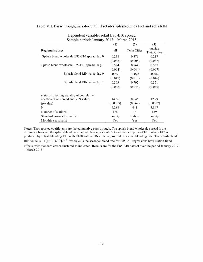
49

Table VII. Pass-through, rack-to-retail, if retailer splash-blends fuel and sells RIN

Dependent variable: retail E85-E10 spread Sample period: January 2012 – March 2015

(1) (2) (3)

Regional subset all Twin Cities outside Twin Cities

Splash blend wholesale E85-E10 spread, lag 0 0.238 0.376 0.217 (0.036) (0.008) (0.037)

Splash blend wholesale E85-E10 spread, lag 1 0.574 0.864 0.537 (0.064) (0.044) (0.067)

Splash blend RIN value, lag 0 -0.353 -0.078 -0.382 (0.047) (0.018) (0.046)

Splash blend RIN value, lag 1 0.393 0.792 0.351 (0.048) (0.046) (0.045)

F statistic testing equality of cumulative coefficient on spread and RIN value 14.66 0.646 12.79 (p-value) (0.0003) (0.569) (0.0007) N 4,288 441 3,847 Number of stations 175 16 159 Standard errors clustered at: county station county Monthly seasonals? Yes Yes Yes

Notes: The reported coefficients are the cumulative pass-through. The splash blend wholesale spread is the difference between the splash-blend wet-fuel wholesale price of E85 and the rack price of E10, where E85 is produced by splash blending E10 with E100 with a RIN at the appropriate seasonal blending rate. The splash blend RIN value is ( ) 6( .1) / .9 D

tPω− − , where ω is the seasonal blend rate for E85. All regressions have station fixed effects, with standard errors clustered as indicated. Results are for the E85-E10 dataset over the period January 2012 – March 2015.

50

Table VIII. RIN pass-through to rack E85-E10 spread and to retail E85-E10 spread

Sample period: January 2012 – March 2015 (1) (2) (3) (4) (5) (6) (7) (8)

regional subset Twin Cities outside Twin Cities Full state Pass through from bulk wholesale to: rack retail retail rack retail retail rack retail

Dependent variable wholesale E85-E10

retail E85 – E10

retail E85 – E10

wholesale E85-E10

retail E85 – E10

retail E85 – E10

wholesale E85-E10

retail E85 – E10

Cumulative pass-through:

Net E85-E10 RIN subsidy, lag 0

0.274 -0.027 0.101 0.226 -0.405 -0.108 0.209 -0.371 (0.341) (0.036) (0.054) (0.080) (0.054) (0.039) (0.079) (0.055)

Net E85-E10 RIN subsidy, lag 1

1.261 0.803 0.988 0.743 0.311 0.522 0.757 0.354 (0.152) (0.049) (0.080) (0.063) (0.046) (0.040) (0.058) (0.050)

Bulk (exchange) E85-E10 cost spread, lag 0

0.721 0.118 0.242 0.586 -0.018 0.164 0.590 -0.004 (0.139) (0.035) (0.014) (0.033) (0.020) (0.016) (0.030) (0.021)

Bulk (exchange) E85-E10 cost spread, lag 1

1.219 0.597 0.765 0.951 0.335 0.596 0.954 0.360 (0.132) (0.061) (0.027) (0.044) (0.040) (0.035) (0.042) (0.041)

F statistic testing coefficient equality on cost, lag 1 = RIN subsidy, lag 1 0.138 3.560 4.284 19.22 0.341 3.19 20.96 0.0218

(p-value) 0.714 0.310 0.287 0.002 0.561 0.079 0.00133 0.883 Clustering for standard

errors: Newey-

West station station rack county county Rack county

N 39 (time series) 441 441 3,847 3,847 3,847 4,288 4,288

Number of stations 16 16 16 159 159 159 175 175 Number of racks 1 1 1 11 11 11 12 12

Monthly seasonals? Yes Yes No Yes Yes No Yes Yes Notes: The reported coefficients are the cumulative pass-through. The RIN subsidy is computed using the seasonal E85 blending ratio. All regressions have station fixed effects, with clustered standard errors as indicated. For Minneapolis-St. Paul, we have only one rack, so regression (1) is a time series regression for that rack with standard errors computed by Newey-West with 4 lags. Results are for the E85-E10 dataset over the period January 2012 – March 2015.