Jim Gatheral (including joint work with Alex Schied) RIO...

Model setup Price manipulation Exponential decay Power-law decay Summary Order books

Price manipulation in models of the order book

Jim Gatheral(including joint work with Alex Schied)

RIO 2009, Buzios, Brasil


Disclaimer

The opinions expressed in this presentation are those of the authoralone, and do not necessarily reflect the views of Bank of AmericaMerrill Lynch, its subsidiaries or affiliates.


Background

In previous work, we showed how the modeling of marketimpact is constrained by requiring no-price-manipulation.

In particular:

If the decay of market impact is exponential, market impactmust be linear in quantity.If decay of market impact is power-law and sensitivity toquantity is also power-law, no-price-manipulation imposesinequality constraints on the exponents.


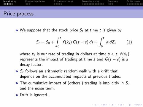
Price process

We suppose that the stock price St at time t is given by

St = S0 +

∫ t

0f (xs) G (t − s) ds +

∫ t

0σ dZs (1)

where xs is our rate of trading in dollars at time s < t, f (xs)represents the impact of trading at time s and G (t − s) is adecay factor.

St follows an arithmetic random walk with a drift thatdepends on the accumulated impacts of previous trades.

The cumulative impact of (others’) trading is implicitly in S0

and the noise term.

Drift is ignored.


We refer to f (·) as the instantaneous market impact functionand to G (·) as the decay kernel.

(1) is a generalization of processes previously considered byAlmgren, Bouchaud and Obizhaeva and Wang.

Remark

The price process (1) is not the only possible generalization ofprice processes considered previously. On the one hand, it seemslike a natural generalization. On the other hand, it is notmotivated by any underlying model of the order book.


Model as limit of discrete time process

The continuous time process (1) can be viewed as a limit of adiscrete time process (see Bouchaud et al. for example):

St =∑i<t

f (δxi ) G (t − i) + noise

where δxi = xi δt is the quantity traded in some small timeinterval δt characteristic of the stock, and by abuse ofnotation, f (·) is the market impact function.

δxi > 0 represents a purchase and δxi < 0 represents a sale.δt could be thought of as 1/ν where ν is the trade frequency.Increasing the rate of trading xi is equivalent to increasing thequantity traded each δt.


Cost of trading

Denote the number of shares outstanding at time t by xt .Then from (1), the cost C [Π] associated with a given tradingstrategy Π = {xt} is given by

C [Π] =

∫ T

0xt dt

∫ t

0f (xs) G (t − s) ds (2)

The dxt = xt dt shares liquidated at time t are traded onaverage at a price

St = S0 +

∫ t

0f (xs) G (t − s) ds

which reflects the residual cumulative impact of all priortrading.


The principle of No Price Manipulation

A trading strategy Π = {xt} is a round-trip trade if∫ T

0xt dt = 0

We define a price manipulation to be a round-trip trade Π whoseexpected cost C [Π] is negative.

The principle of no-price-manipulation

Price manipulation is not possible.

Remark

If price manipulation were possible, the optimal strategy would notexist.


A specific strategy

Consider a strategy where shares are accumulated at the (positive)constant rate v1 and then liquidated again at the (positive)constant rate v2. According to equation (2), the cost of thisstrategy is given by C11 + C22 − C12 with

C11 = v1 f (v1)

∫ θT

0dt

∫ t

0G (t − s) ds

C22 = v2 f (v2)

∫ T

θTdt

∫ t

θTG (t − s) ds

C12 = v2 f (v1)

∫ T

θTdt

∫ θT

0G (t − s) ds (3)

where θ is such that v1 θT − v2 (T − θT ) = 0 so

θ =v2

v1 + v2


Special case: Trade in and out at the same rate

One might ask what happens if we trade into, then out of aposition at the same rate v . If G (·) is strictly decreasing,

C [Π] = v f (v)

{∫ T/2

0

dt

∫ t

0

G (t − s) ds +

∫ T

T/2

dt

∫ t

T/2

G (t − s) ds

−∫ T

T/2

dt

∫ T/2

0

G (t − s) ds

}

= v f (v)

{∫ T/2

0

dt

∫ t

0

[G (t − s)− G (t + T/2− s)] ds

+

∫ T

T/2

dt

∫ t

T/2

[G (t − s)− G (T − s)] ds

}> 0

We conclude that if price manipulation is possible, it mustinvolve trading in and out at different rates.


Exponential decay

Suppose that the decay kernel has the form

G (τ) = e−ρ τ

Then, explicit computation of all the integrals in (3) gives

C11 = v1 f (v1)1

ρ2

{e−ρ θT − 1 + ρ θT

}C12 = v2 f (v1)

1

ρ2

{1 + e−ρT − e−ρ θT − e−ρ (1−θ) T

}C22 = v2 f (v2)

1

ρ2

{e−ρ (1−θ) T − 1 + ρ (1− θ) T

}(4)

We see in particular that the no-price-manipulation principle forcesa relationship between the instantaneous impact function f (·) andthe decay kernel G (·).


Exponential decay

After making the substitution θ = v2/(v1 + v2) and imposing theprinciple of no-price-manipulation, we obtain

v1 f (v1)

[e− v2 ρ

v1+v2 − 1 +v2 ρ

v1 + v2

]+v2 f (v2)

[e− v1 ρ

v1+v2 − 1 +v1 ρ

v1 + v2

]−v2 f (v1)

[1 + e−ρ − e

− v1 ρ

v1+v2 − e− v2 ρ

v1+v2

]≥ 0 (5)

where, without loss of generality, we have set T = 1. We note thatthe first two terms are always positive so price manipulation is onlypossible if the third term (C12) dominates the others.


Example: f (v) =√

v

Let v1 = 0.2, v2 = 1, ρ = 1. Then the cost of liquidation is givenby

C = C11 + C22 − C12 = −0.001705 < 0

Since ρ really represents the product ρT , we see that for anychoice of ρ, we can find a combination {v1, v2,T} such that around trip with no net purchase or sale of stock is profitable. Weconclude that if market impact decays exponentially, theno-price-manipulation principle excludes a square rootinstantaneous impact function.

Can we generalize this?


Expansion in ρ

Expanding expression (5) in powers of ρ, we obtain

v1 v2 [v1 f (v2)− v2 f (v1)] ρ2

2(v1 + v2)2+ O

(ρ3)≥ 0

We see that price manipulation is always possible for small ρ unlessf (v) is linear in v and we have

Lemma

Under exponential decay of market impact, no-price-manipulationimplies f (v) ∝ v.


Empirical viability of exponential decay of market impact

Empirically, market impact is concave in v for small v .

Also, market impact must be convex for very large v

Imagine submitting a sell order for 1 million shares when thereare bids for only 100,000.

We conclude that the principle of no-price-manipulationexcludes exponential decay of market impact for anyempirically reasonable instantaneous market impact functionf (·).


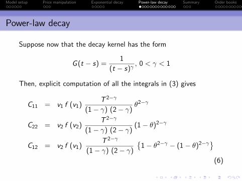
Power-law decay

Suppose now that the decay kernel has the form

G (t − s) =1

(t − s)γ, 0 < γ < 1

Then, explicit computation of all the integrals in (3) gives

C11 = v1 f (v1)T 2−γ

(1− γ) (2− γ)θ2−γ

C22 = v2 f (v2)T 2−γ

(1− γ) (2− γ)(1− θ)2−γ

C12 = v2 f (v1)T 2−γ

(1− γ) (2− γ)

{1− θ2−γ − (1− θ)2−γ}

(6)


Power-law decay

According to the principle of no-price-manipulation , substitutingθ = v2/(v1 + v2), we must have

f (v1){v1 v2

1−γ − (v1 + v2)2−γ + v12−γ + v2

2−γ}+f (v2) v12−γ ≥ 0

(7)

If γ = 0, the no-price-manipulation condition (7) reduces to

f (v2) v1 − f (v1) v2 ≥ 0

so again, permanent impact must be linear.

If γ = 1, equation (7) reduces to

f (v1) + f (v2) ≥ 0

So long as f (·) ≥ 0, there is no constraint on f (·) when γ = 1.


The limit v1 � v2 and 0 < γ < 1

In this limit, we accumulate stock much more slowly than weliquidate it. Let v1 = ε v and v2 = v with ε� 1. Then, in thelimit ε→ 0, with 0 < γ < 1, equation (7) becomes

f (ε v){ε− (1 + ε)2−γ + ε2−γ + 1

}+ f (v) ε2−γ

∼ −f (ε v) (1− γ) ε+ f (v) ε2−γ ≥ 0

so for ε sufficiently small we have

f (ε v)

f (v)≤ ε1−γ

1− γ(8)

If the condition (8) is not satisfied, price manipulation is possibleby accumulating stock slowly, maximally splitting the trade, thenliquidating it rapidly.


Power-law impact: f (v) ∝ v δ

If f (v) ∼ v δ (as per Almgren et al.), the no-price-manipulationcondition (8) reduces to

ε1−γ−δ ≥ 1− γ

and we obtain

Small v no-price-manipulation condition

γ + δ ≥ 1


Cost of VWAP with power-law market impact and decay

From equation (6), the cost of an interval VWAP execution withduration T is proportional to

C = v f (v) T 2−γ

Noting that v = n/T , and putting f (v) ∝ (v/V )δ, the cost pershare is proportional to ( n

V

)δT 1−γ−δ

If γ + δ = 1, the cost per share is independent of T and inparticular, if γ = δ = 1/2, the impact cost per share is proportionalto√

n/V , which is the well-known square-root formula for marketimpact as described by, for example, Grinold and Kahn.


The square-root formula, γ and δ

The square-root market impact formula has been widely usedin practice for many years.

If correct, this formula implies that the cost of liquidating astock is independent of the time taken.

Fixing market volume and volatility, impact depends only size.

We can check this prediction empirically.

See for example Engle, Ferstenberg and Russell, 2008.

Also, according to Almgren, δ ≈ 0.6 and according toBouchaud γ ≈ 0.4.

Empirical observation

δ + γ ≈ 1!


The shape of the order book

Bouchaud, Mezard and Potters (2002) derive the followingapproximation to the average density ρ(∆) of orders as a functionof a rescaled distance ∆ from the price level at which the order isplaced to the current price:

ρ(∆) = e−∆

∫ ∆

0du

sinh(u)

u1+µ+ sinh(∆)

∫ ∞∆

due−u

u1+µ(9)

where µ is the exponent in the empirical power-law distribution ofnew limit orders.


Approximate order density

The red line is a plot of the order density ρ(∆) with µ = 0.6 (asestimated by Bouchaud, Mezard and Potters).

0 2 4 6 8 10

0.0

0.5

1.0

1.5

!

"(!)


Virtual price impact

Switching x− and y−axes in a plot of the cumulative order density givesthe virtual impact function plotted below. The red line corresponds toµ = 0.6 as before.

02

46

810

Quantity: !"0

#$(u)du

Price

impa

ct: #


Impact for high trading rates

You can’t trade more than the total depth of the book soprice impact increases without limit as n→ nmax .

For a sufficiently large trading rate v , it can be shown that

f (v) ∼ 1

(1− v/vmax)1/µ

Setting v = vmax (1− ε) and taking the limit ε→ 0,

f (v) ∼ 1

ε1/µas ε→ 0.

Imagine we accumulate stock at a rate close to vmax := 1 andliquidate at some (lower) rate v .

This is the pump and dump strategy!


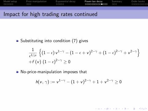
Impact for high trading rates continued

Substituting into condition (7) gives

1

ε1/µ

{(1− ε) v1−γ − (1− ε+ v)2−γ + (1− ε)2−γ + v2−γ

}+f (v) (1− ε)2−γ ≥ 0

No-price-manipulation imposes that

h(v , γ) := v1−γ − (1 + v)2−γ + 1 + v2−γ ≥ 0


Graphical illustration

0.0 0.2 0.4 0.6 0.8 1.0

-0.3

-0.2

-0.1

0.0

0.1

0.2

0.3

v

h(v,

γ)

γ = 2 − log(3) log(2)

γ = 0.5

γ = 0.3


Large size no price manipulation condition

From the picture, we see that h(v , γ) ≥ 0 implies

Large size no price manipulation condition

γ > γ∗ = 2− log 3

log 2


Long memory of order flow

It is empirically well-established that order-flow is a longmemory process.

More precisely, the autocorrelation function of order signsdecays as a power-law.There is evidence that this autocorrelation results from ordersplitting.

Imposing linear growth of return variance in trading time(Bouchaud et al. 2004) in an effective model such as (1)forces power-law decay of market impact with exponentγ ≤ 1/2.


Summary of prior work

By imposing the principle of no-price-manipulation, we showedthat if market impact decays as a power-law 1/(t − s)γ andthe instantaneous market impact function is of the formf (v) ∝ v δ, we must have

γ + δ ≥ 1

We excluded the combination of exponential decay withnonlinear market impact.


We observed that if the average cost of a (not-too-large)VWAP execution is roughly independent of duration, theexponent δ of the power law of market impact should satisfy:

δ + γ ≈ 1

By considering the tails of the limit-order book, we deducethat

γ ≥ γ∗ := 2− log 3

log 2≈ 0.415

Long memory of order flow imposes γ ≤ 1/2.


Schematic presentation of constraints

0.0 0.5 1.0 1.5

0.0

0.5

1.0

1.5

!

"

0.0 0.5 1.0 1.5

0.0

0.5

1.0

1.5

! + " # 1

! # !*

! $ 1 2

! = 0.4, " = 0.6! = 0.5, " = 0.5


The model of Alfonsi, Fruth and Schied

Alfonsi, Fruth and Schied (2009) consider the following (AS)model of the order book:

There is a continuous (in general nonlinear) density of ordersf (x) above some martingale ask price At . The cumulativedensity of orders up to price level x is given by

F (x) :=

∫ x

0f (y) dy

Executions eat into the order book (i.e. executions are withmarket orders).

A purchase of ξ shares at time t causes the ask price toincrease from At + Dt to At + Dt+ with

ξ =

∫ Dt+

Dt

f (x) dx = F (Dt+)− F (Dt)


We can define a volume impact process

Et := F (Dt)

which represents how much of the book has been eaten up byexecutions up to time t.

Depending on the model, either the spread Dt or the volumeimpact process Et revert exponentially at some rate ρ.

This captures the resiliency of the order book: Limit ordersarrive to replenish order density lost through executions.


Schematic of the model

Order density f(x)

f(Dt)

f(Dt+)

Et+ −Et

0 Dt Dt+

Et

Price level

When a trade of size ξ is placed at time t,

Et 7→ Et+ = Et + ξ

Dt = F−1(Et) 7→ Dt+ = F−1(Et+) = F−1(Et + ξ)


Example: The model of Obizhaeva and Wang

Obizhaeva and Wang (2005) consider a block-shaped order bookwith constant order density.

Order density f(x)f(Dt) f(Dt+)

Et+ −Et

0 Dt Dt+

Et

Price level


In the Obizhaeva Wang (OW) model, we thus have

f (x) = 1

F (x) = x

Et = Dt

∆Dt := Dt+ − Dt = ξ

Thus market impact ∆Dt is linear in the quantity ξ. Betweenexecutions, the spread Dt and the volume impact process Et bothdecay exponentially at rate ρ so that at time t after an executionat the earlier time s, we have

Dt = Ds+ e−ρ (t−s)


Cost of execution and optimal trading strategy

Given a trading strategy Π with trading at the rate xt , the cost ofexecution in the OW model is given by

C(Π) =

∫ T

0xt dt

∫ t

0xs e−ρ (t−s) ds

When the trading policy xt = ut is statically optimal, theEuler-Lagrange equation applies:

∂

∂t

δCδut

= 0

Then, for some constant A, we have

δCδut

=

∫ t

0us e−ρ (t−s) ds +

∫ T

tus e−ρ (s−t) ds = A (10)


Substitutingut = δ(t) + ρ+ δ(T − t)

where δ(·) is the Dirac delta function into (10) gives

δCδut

=

∫ t

0us e−ρ (t−s) ds +

∫ T

tus e−ρ (s−t) ds

= e−ρ t +

∫ t

0ρ e−ρ (t−s) ds +

∫ T

tρ e−ρ (s−t) ds + e−ρ (T−t)

= 2

so ut is the optimal strategy.

The optimal strategy

Trade blocks of stock at times t = 0 and t = T and tradecontinuously at rate ρ between these two times.


No price manipulation

The optimal strategy involves only purchases of stock, nosales.

Thus there cannot be price manipulation in the OW model.

The OW price process is a special case of (1) with linear priceimpact and exponential decay of market impact.

Consistent with our lemma, there is no price manipulation.

The OW model is also a special case of the AS model.


Cost of execution in the AS model

In general, the cost of trade execution in the AS model has acontinuous piece and a discrete piece:

C(Π) =

∫ T

0xt F−1(Et) dt +

∑t≤T

[H(Et+)− H(Et)] (11)

where

H(x) =

∫ x

0F−1(x) dx

and

Et =

∫ t


is the volume impact process.


Optimal strategy in the AS model

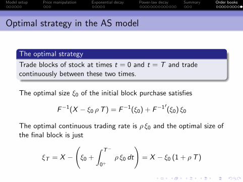
The optimal strategy

Trade blocks of stock at times t = 0 and t = T and tradecontinuously between these two times.

The optimal size ξ0 of the initial block purchase satisfies

F−1(X − ξ0 ρT ) = F−1(ξ0) + F−1′(ξ0) ξ0

The optimal continuous trading rate is ρ ξ0 and the optimal size ofthe final block is just

ξT = X −

(ξ0 +

∫ T−

0+

ρ ξ0 dt

)= X − ξ0 (1 + ρT )


No price manipulation

Once again, the optimal strategy involves only purchases ofstock, no sales.

Thus there cannot be price manipulation in the AS model.

What’s going on?

“Under exponential decay of market impact, no-price-manipulationimplies f (v) ∝ v”


A potential conundrum

From Alfonsi and Schied (2009)

“Our result on the non-existence of profitable price manipulationstrategies strongly contrasts Gatheral’s conclusion that thewidely-assumed exponential decay of market impact is compatibleonly with linear market impact.”

“The preceding corollary shows that, in our Model 1, exponentialresilience of price impact is well compatible with nonlinear impact...This fact is in stark contrast to Gatheral’s observation that, in arelated but different continuous-time model, exponential decay ofprice impact gives rise to price manipulation as soon as priceimpact is nonlinear. ”


Expected price in the two models

Recall from the price process (1) that in our model:

E[St ] =

∫ t


In the AS model, the current spread Dt and the volume impactprocess Et are related as

Dt = F−1(Et)

so effectively, for continuous trading strategies,

E[St ] = F−1

(∫ t


)


Cost of trading

The expected cost of trading in the two models is then given by

CJG =

∫ T

0xt dt

∫ t


and

CAS =

∫ T

0xt dt F−1

(∫ t


)These two expression are identical in the OW case with

F (x) = x ; f (v) = v ; G (t − s) = e−ρ (t−s)

For more general F (·), the models are different.


VWAP equivalent models

Are there choices of F (·) for which we can match the expectedcost of a VWAP in the two models?

For a VWAP execution, we have xt = v , a constant. Then

CJG = v f (v)

∫ T

0dt

∫ t

0G (t − s) ds

and

CAS = v

∫ T

0dt F−1

(v

∫ t

0e−ρ (t−s) ds

)It turns out that CJG = CAS for all v if and only if F−1(x) = xδ,f (v) = v δ and

G (τ) =δ ρ e−ρ τ

(1− e−ρ τ )1−δ


Thus for small τ ,

G (τ) ∼ δ ρ

(ρ τ)γ

with γ = 1− δ and for large τ ,

G (τ) ∼ δ ρ e−ρ τ

Resolution

With power-law market impact ∝ v δ, and exponential resilience,decay of market impact is power-law with exponent γ = 1− δ.

Remark

The relationship δ + γ = 1 between the exponents emergesnaturally from a simple model of the order book!


Conclusion

There is no contradiction.

Exponential resilience of an order book with power-law shapeinduces power-law decay of market impact (at least for shorttimes).

Both AS-style models and processes like (1) aregeneralizations of Obizhaeva and Wang’s model.

The AS models are motivated by considerations of dynamics ofthe order book.The class of AS models with exponential resilience has beenshown to be free of price manipulation.

Our results suggest that the empirically observed relationshipδ + γ ≈ 1 may reflect properties of the order book rather thansome self-organizing principle.


Next steps

Generalize to non-exponential order book resilience.

Investigate properties of optimal strategies.

Derive conditions for no price manipulation in the generalcase.


References

Aurelien Alfonsi, Antje Fruth and Alexander Schied.

Optimal execution strategies in limit order books with general shape functions.Quantitative Finance, 2009.

Aurelien Alfonsi and Alexander Schied.

Optimal execution and absence of price manipulations in limit order book models.Technical paper, 2009.

Robert Almgren, Chee Thum, Emmanuel Hauptmann, and Hong Li.

Equity market impact.Risk, July:57–62, July 2005.

Jean-Philippe Bouchaud, Yuval Gefen, Marc Potters, and Matthieu Wyart.

Fluctuations and response in financial markets: the subtle nature of ‘random’ price changes.Quantitative Finance, 4:176–190, April 2004.

Jean-Philippe Bouchaud, Marc Mezard, and Marc Potters.

Statistical properties of stock order books: empirical results and models.Quantitative Finance, 2:251–256, August 2002.


Robert F. Engle, Robert Ferstenberg, and Jeffrey Russell.

Measuring and modeling execution cost and risk.Technical report, University of Chicago Graduate School of Business, 2008.

Jim Gatheral.

No-dynamic-arbitrage and market impact .Forthcoming Quantitative Finance.

Richard C. Grinold and Ronald N. Kahn.

Active Portfolio Management.New York: The McGraw-Hill Companies, Inc., 1995.

Anna Obizhaeva and Jiang Wang.

Optimal trading strategy and supply/demand dynamics.Technical report, MIT Sloan School of Management, 2005.

Jim Gatheral (including joint work with Alex Schied) RIO...

Documents

Transcript of Jim Gatheral (including joint work with Alex Schied) RIO...