JHE/jyc R.07-01-041 R. Olivia Samad - California
175
R. Olivia Samad Attorney [email protected] P.O. Box 800 2244 Walnut Grove Ave. Rosemead, California 91770 (626) 302-3477 Fax (626) 302-7740 November 30, 2010 Ms. Julie Fitch Director, Energy Division California Public Utilities Commission 505 Van Ness Avenue San Francisco, CA 94102 Re: A.08-06-001 - Statewide Joint Utility Study of Permanent Load Shifting Dear Ms. Fitch: Enclosed is the Statewide Joint Investor-Owned Utility (IOU) Study of Permanent Load Shifting pursuant to Ordering Paragraph No. 32 of Decision 09-08-027, which states: “Pacific Gas and Electric Company, Southern California Edison Company, and San Diego Gas & Electric Company shall work with parties to examine ways of expanding the availability of permanent load shifting. This study shall include discussion of a standard offer proposal that could apply generally to any permanent load shifting technologies including, but not limited to, thermal energy storage. This study should also consider other ways of encouraging permanent load shifting, including modifications to time of use rates or another RFP process. This report shall contain a summary of permanent load shifting standard offers available throughout the United States, as well as an evaluation of what incentive payment would be appropriate for a future standard offer. Each of the utilities shall provide its report to the Director of the Energy Division no later than December 1, 2010, and shall provide copies to the most recent service list in this proceeding. In addition, the utilities shall post these reports on a publicly available web site.” By December 1, 2010, the report will be posted on the following publicly available website run by E3, the author of this study: http://www.ethree.com/public_projects/sce1.html . Sincerely, /s/ R. Olivia Samad R. Olivia Samad cc: All Parties of Record in A.08-06-001 via email RMS: as#1771037 Enclosure(s) JHE/jyc R.07-01-041 ATTACHMENT 1 F I L E D 02-11-11 01:25 PM
Transcript of JHE/jyc R.07-01-041 R. Olivia Samad - California
R. Olivia Samad Attorney [email protected]
P.O. Box 800 2244 Walnut Grove Ave. Rosemead, California 91770 (626) 302-3477 Fax (626) 302-7740
November 30, 2010
Ms. Julie Fitch Director, Energy Division California Public Utilities Commission 505 Van Ness Avenue San Francisco, CA 94102
Re: A.08-06-001 - Statewide Joint Utility Study of Permanent Load Shifting
Dear Ms. Fitch:
Enclosed is the Statewide Joint Investor-Owned Utility (IOU) Study of Permanent Load Shifting pursuant to Ordering Paragraph No. 32 of Decision 09-08-027, which states: “Pacific Gas and Electric Company, Southern California Edison Company, and San Diego Gas & Electric Company shall work with parties to examine ways of expanding the availability of permanent load shifting. This study shall include discussion of a standard offer proposal that could apply generally to any permanent load shifting technologies including, but not limited to, thermal energy storage. This study should also consider other ways of encouraging permanent load shifting, including modifications to time of use rates or another RFP process. This report shall contain a summary of permanent load shifting standard offers available throughout the United States, as well as an evaluation of what incentive payment would be appropriate for a future standard offer. Each of the utilities shall provide its report to the Director of the Energy Division no later than December 1, 2010, and shall provide copies to the most recent service list in this proceeding. In addition, the utilities shall post these reports on a publicly available web site.”
By December 1, 2010, the report will be posted on the following publicly available website run by E3, the author of this study: http://www.ethree.com/public_projects/sce1.html.
Sincerely,
/s/ R. Olivia Samad
R. Olivia Samad
cc: All Parties of Record in A.08-06-001 via email RMS: as#1771037
Enclosure(s)
JHE/jyc R.07-01-041 ATTACHMENT 1
F I L E D02-11-1101:25 PM

Appendix A
Statewide Joint IOU Study of Permanent Load Shifting
JHE/jyc R.07-01-041

Page 1
�
��
Statewide�Joint�IOU�Study��
of�Permanent�Load�Shifting��
�
�
Prepared�for:��
Southern�California�Edison,��
Pacific�Gas�and�Electric,�
San�Diego�Gas�and�Electric��
�
�
November�29,�2010�
�
�
�
�
JHE/jyc R.07-01-041

Table of Contents
1. Executive Summary .................................................................................................... 4 1.1. Definition of PLS ................................................................................................. 4 1.2. PLS Cost-Effectiveness ........................................................................................ 6 1.3. Value Proposition to End-User .......................................................................... 10 1.4. PLS Market Assessment ..................................................................................... 12 1.5. PLS Program Recommendations ....................................................................... 13
2. Introduction and Purpose of Study ........................................................................... 18 2.1. Policy Background ............................................................................................. 18
2.1.1. CPUC Regulatory Background ................................................................... 18 2.1.2. Other Policy Background ............................................................................ 21
2.2. PLS Pilots ........................................................................................................... 21 2.2.1. SCE ............................................................................................................. 21 2.2.2. PG&E .......................................................................................................... 22 2.2.3. SDG&E ....................................................................................................... 23
2.3. Definition of PLS ............................................................................................... 23 3. Study Methodology ................................................................................................... 26
3.1. Cost effectiveness ............................................................................................... 27 3.1.1. PLS Modeling Inputs .................................................................................. 27 3.1.2. Cost-effectiveness Tests .............................................................................. 29 3.1.3. PLS Avoided Cost Benefits ........................................................................ 32 3.1.4. Key Sensitivities ......................................................................................... 37 3.1.5. Broad Scenario Analysis (“Matrix”) ........................................................... 39 3.1.6. Cost effectiveness of individual cases ........................................................ 42 3.1.7. Specific Case Studies: Simulated Installations ........................................... 43 3.1.8. Specific Case Studies: IOU PLS Pilots and Recent Installations ............... 45
3.2. End-user Value Proposition ............................................................................... 46 3.3. Market Assessment ............................................................................................ 48
4. Modeling Results ...................................................................................................... 50 4.1. Cost-effectiveness .............................................................................................. 50
4.1.1. Avoided Cost Benefit Matrix ...................................................................... 50 4.1.2. Bill Savings and Rate Payer Neutral Incentive ........................................... 51 4.1.3. Sensitivity Analyses .................................................................................... 53 4.1.4. Specific Case Results: Simulated Scenarios ............................................... 68 4.1.5. Specific Case Results: PLS Pilots and Recent Installations ....................... 71 4.1.6. Case Studies: Generation Capacity Value Sensitivities .............................. 80
4.2. End User Impacts ............................................................................................... 82 4.2.1. Project Paybacks before Incentives ............................................................ 82 4.2.2. Incentive Level Requirements .................................................................... 84 4.2.3. Sensitivities to Incentive Level Requirements ............................................ 86
5. Market Issues and Stakeholder Feedback ................................................................. 89 5.1. State of the Industry ........................................................................................... 89
5.1.1. Permanent Load Shifting Programs ............................................................ 89 5.1.2. Stakeholder Feedback ................................................................................. 99
6. Program Design Recommendations ........................................................................ 106
JHE/jyc R.07-01-041

Statewide Joint IOU Study of Permanent Load Shifting
Energy and Environmental Economics, Inc Page 2 2
6.1. Overall Cost-effectiveness of PLS ................................................................... 106 6.1.1. Total Resource Cost Test .......................................................................... 106 6.1.2. Considerations for a Market Transforming PLS Program ........................ 109 6.1.3. Conclusions Based on the TRC Test ........................................................ 110
6.2. PLS Program Design Framework – Standard Offer ......................................... 111 6.3. PLS Program Design Characteristics ............................................................... 114
6.3.1. System Design .......................................................................................... 116 6.3.2. Build and Performance Test ...................................................................... 117 6.3.3. Operations ................................................................................................. 118
6.4. Establishing Incentive Levels for Standard Offer ............................................ 118 6.4.1. Ratepayer Neutral Incentive Levels .......................................................... 119 6.4.2. Incentive Levels based on Expected Payback .......................................... 122 6.4.3. Considerations for RFP- based Program Designs ..................................... 123 6.4.4. Considerations on Retail Rate Design ...................................................... 124 6.4.5. Performance Based Incentives .................................................................. 125
7. Bibliography ........................................................................................................... 126Appendix A: Avoided Costs ..…………………………………………………………A-1 Appendix B: Stakeholder Feedback …………………………………………………...B-1
JHE/jyc R.07-01-041

Statewide Joint IOU Study of Permanent Load Shifting
Energy and Environmental Economics, Inc Page 3 3
Glossary
CE Cost effectiveness
CEC California Energy Commission
CPUC California Public Utility Commission
DR Demand Response
DSIRE Database of State Incentives for Renewable Energy
EM&V Evaluation, Measurement and Verification
IMIOC Internal melt ice on coil
ISAC Ice storage air conditioning
PAC Program Administrator Cost Test
PG&E Pacific Gas and Electric Company
PLS Permanent load shifting
RIM Ratepayer impact measure test
SCE Southern California Edison
SCHW Stratified chilled water
SDG&E San Diego Gas and Electric
TES Thermal energy storage
Ton-hour Unit of cooling energy (equivalent to 12,000 BTUs)
TOU Time of use
TRC Total resource cost test
JHE/jyc R.07-01-041

Statewide Joint IOU Study of Permanent Load Shifting
Energy and Environmental Economics, Inc Page 4 4
1. Executive Summary
The purpose of this study is to investigate cost-effectiveness and program design
to expand the use of permanent load shifting (PLS) within the SCE, PG&E, and
SDG&E service territories (“Joint Utilities”). PLS refers to a broad set of
technologies that shift electricity use from peak to off-peak periods. This report
is an outcome of the California Public Utility Commission (CPUC) Order
D.09-08-027 “Decision adoption demand response activities and budgets for
2009 through 2011” and will provide more information to the Joint Utilities on
PLS for use in preparing proposed Demand Response programs including PLS to
the CPUC.
Energy and Environmental Economics, Inc. (E3) and StrateGen Consulting were
selected by the Joint Utilities and the CPUC to conduct this study. E3 and
StrateGen Consulting (the “project team”) used a collaborative stakeholder
process with two workshops, numerous stakeholder interviews and meetings,
and the release of a publicly available cost-effectiveness tool to develop the
study results. The project team also gathered and used data from each of the
utility PLS Pilot Programs, and technology vendor data in the public domain and
under Non-Disclosure Agreements (NDAs).
As described in this report, the study addresses the following areas;
� Definition of Permanent Load Shifting
� Cost-effectiveness of PLS
� PLS Program ‘Best Practices” and Stakeholder Input
� Proposed PLS Program Design Elements, including Standard Offer
1.1. Definition of PLS
For the purposes of this study, the project team proposed and uses a broad
definition of PLS. With support of the stakeholder group, a ‘technology neutral’
JHE/jyc R.07-01-041
Statewide Joint IOU Study of Permanent Load Shifting
Energy and Environmental Economics, Inc Page 5 5
definition was proposed based on the impact of the electricity usage profile
rather than the technology used to create the impact. Additional guiding
principles include business/ownership neutrality, and the measurable shift at
program level for evaluation, measurement and verification. PLS is defined with
the overarching goal of “routine shifting from one time period to another during
the course of a day to help meet peak loads during periods when energy use is
typically high and improve grid operations in doing so (economics, efficiency,
and/or reliability).”
The type of load shape impact that meets the PLS definition can be delivered by
technologies in three broad categories; electrical energy storage, thermal energy
storage, and process shifting (see Table 1). Each technology category and
individual technologies within each class have their own unique costs, benefits,
strengths and limitations. For example, some of the technologies are mature
and in wide use, such as thermal storage systems for building cooling systems,
and some are still emerging such as electric battery storage; some provide a
‘static’ set shift in load pattern, while others can provide a ‘dynamic’ response
based on electric system conditions. There are also process shifting efforts that
involve rescheduling the use of electricity. For all of these categories, it will be
extremely challenging to create a single, simple, technology neutral PLS program
design that appropriately addresses the differences in the costs and benefits of
the technologies to establish a common design framework.
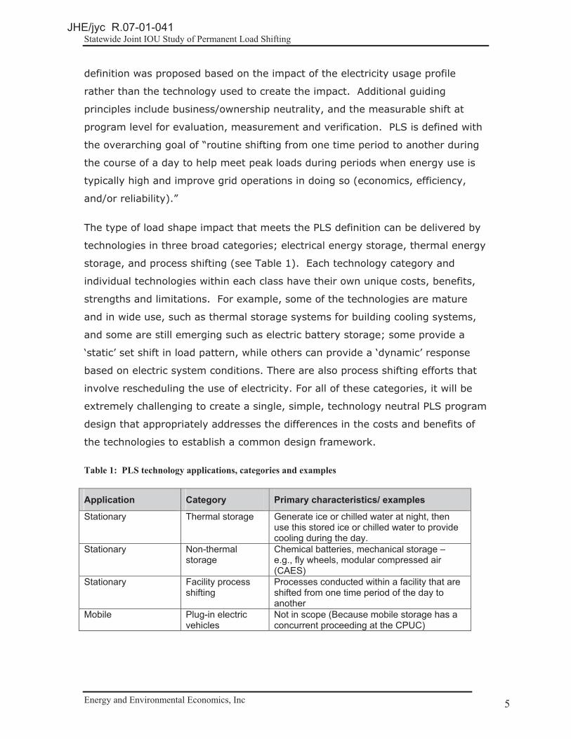
Table 1: PLS technology applications, categories and examples
Application Category Primary characteristics/ examples
Stationary Thermal storage Generate ice or chilled water at night, then use this stored ice or chilled water to provide cooling during the day.
Stationary Non-thermal storage
Chemical batteries, mechanical storage – e.g., fly wheels, modular compressed air (CAES)
Stationary Facility process shifting
Processes conducted within a facility that are shifted from one time period of the day to another
Mobile Plug-in electric vehicles
Not in scope (Because mobile storage has a concurrent proceeding at the CPUC)
JHE/jyc R.07-01-041

Statewide Joint IOU Study of Permanent Load Shifting
Energy and Environmental Economics, Inc Page 6 6
While the PLS definition is broad, there are many elements that this report has
found to be outside the scope of PLS. First, PLS is not solely event-based
demand response. Second, PLS is not behavior-based energy efficiency. PLS is
provided and quantified by discrete equipment or controls, not solely by general
customer behavior modification, and it does not reduce the level of customer
service. Third, the load reduction and shifting that can be achieved by best
practices commissioning, retro-commissioning or adjustment of controls is not
considered PLS, unless such practices are being applied directly to existing
legacy PLS technologies (such as unused thermal storage tanks) and are not
currently being implemented through energy efficiency programs. We also
exclude, by stakeholder consensus, the inclusion of electric vehicles in PLS.
Finally, PLS is not achieved through fuel switching.
1.2. PLS Cost-Effectiveness
The project team emphasized the importance of cost-effectiveness of PLS
throughout the development of the study. E3 focused on the overall societal and
ratepayer cost-effectiveness of PLS given current California electricity market
conditions, and StrateGen Consulting focused on the value proposition to the
end-user and whether a given PLS program design was likely to result in
significant adoptions. This approach was designed to provide more information
to the Joint Utilities as they decide the scope and scale of their proposed PLS
programs and to provide more information for establishing incentive levels that
balance the costs to ratepayers and expected program adoption rates.
To value the benefits of PLS to ratepayers, and to California as a whole, E3
developed a PLS cost effectiveness framework that is similar to the framework
used to evaluate the benefits of utility distributed generation programs such as
the California Solar Initiative (CSI) and the Self-Generation Incentive Program
(SGIP) [Decision 09-08-026, August 20, 2009]1. A similar framework is also
currently being considered for use in evaluating the cost-effectiveness of demand
1 http://docs.cpuc.ca.gov/published/FINAL_DECISION/105926.htm
JHE/jyc R.07-01-041

Statewide Joint IOU Study of Permanent Load Shifting
Energy and Environmental Economics, Inc Page 7 7
response [R. 07-01-014]. The precursor to each of these was the development
of avoided costs for energy efficiency adopted by the CPUC in 2004 and 2005
[R.04-04-025]2.
The avoided cost benefits provided by PLS include electrical energy, losses,
ancillary services, system (generation) capacity, transmission and distribution
capacity, environmental costs, and avoided renewable energy purchases. We
also investigated the renewable integration benefits of load following and over-
generation that could be provided by PLS.
As shown in Figure 1, using this new PLS cost effectiveness framework, the
lifecycle value of the avoided cost benefits of PLS technologies (assuming 15
year project life estimates) is in the range of $500/peak kW to $2500/peak kW,
depending on the number of hours the PLS system can shift load, and what hour
the load shifting starts. These figures are calculated based on the kW value of
the load shift and are ‘technology neutral’, and do not include benefits from
other value streams. They assume the ‘best case’ operational profile in that they
assume the maximum load shift every day of the year, and off-peak usage at the
least cost period during the night. For example, a 6 hour load reduction
beginning at 12pm over an assumed 15-year life is valued at ~ $2200/kW (or
$365/kWh stored capacity).
2 http://docs.cpuc.ca.gov/word_pdf/FINAL_DECISION/36203.pdf
JHE/jyc R.07-01-041

Statewide Joint IOU Study of Permanent Load Shifting
Energy and Environmental Economics, Inc Page 8 8
Figure 1: Broad Scenario Analysis – Avoided Costs
$0
$500
$1,000
$1,500
$2,000
$2,500
$3,000
7 8 9 10 11 12 13 14 15 16 17
Avoi
ded�
Cost
�Ben
efits
�$/k
W�P
eak�
Capa
city
�Re
duct
ion
Shift�Start�Hour
1�Hour
2�Hours
4�Hours
6�Hours
8�Hours
10�Hours
While the project team believes these figures are appropriate for currently
available PLS technologies, we note that the benefits in Figure 1 do not include
the provision of ancillary services such as regulation that some PLS technologies
plan to provide3. In addition, some stakeholders have suggested that a 15-year
life is too short and longer lived installations will have greater lifecycle value.
To address these issues, the report presents these sensitivities and many others.
For example, an assumed 30 year project life cycle is estimated to increase
lifecycle avoided cost benefits by approximately 30%. The main results are also
shown in terms of lifecycle $/kWh-stored, which is a common capacity metric for
batteries. In addition, the “in-situ” cost-effectiveness of both simulated and real
installations (such as from the utility PLS pilots) are provided.
Using the California Standard Practice Manual (SPM) framework for evaluating
the cost effectiveness of ratepayer funded programs that the CPUC relies on for
3 A number of battery technologies providers have indicated their ability and interest to provide ancillary services as well as load shifting.
JHE/jyc R.07-01-041

Statewide Joint IOU Study of Permanent Load Shifting
Energy and Environmental Economics, Inc Page 9 9
other distributed resources, the installed PLS system costs must be less than the
lifecycle benefits in order to pass the Total Resource Cost (TRC) test. While the
installed system costs specific to PLS are often difficult to ascertain (for example,
due to customer confidentiality), or the costs were obtained under a
nondisclosure agreement (NDA) and cannot be shared in this report, certain
classes of thermal storage are likely to pass the TRC (e.g., warehouse precooling
achieved by controls modifications, improvement of existing thermal storage
systems, medium-sized ice-based storage, chilled water for new construction and
expansion applications), as these technologies are more mature and their
lifecycle values are within the range of the avoided cost benefits. Emerging grid
connected battery technologies and smaller scale4 thermal storage systems with
higher costs are less likely to pass the TRC cost-effectiveness test at their
current system costs.
One of the objectives of this study was to determine what level of incentive
payment would be appropriate. From a ratepayer perspective, an incentive can
be provided to reduce the incremental costs of PLS systems over standard non-
PLS technology without any ‘cross-subsidy’ at a level equal to the lifecycle
benefits presented in Figure 1 less the bill savings the end-user receives by
operating the PLS system. One can think of the bill savings as ‘paying’ the end-
user for the societal benefits they provide with their PLS system. This study
finds that even when the PLS operations are designed to maximize bill savings,
there are some situations when an incentive payment can be provided without
any cross-subsidy. The actual value of this ‘ratepayer neutral’ incentive level
depends on the PLS system operation and the specific retail tariff.
Using a ‘generic’ rate that reflects the rate structure the Joint Utilities have for
medium and large commercial customers we find an incentive payment of
$75/peak kW to $800/peak kW for PLS is possible without any cross-subsidy
(this may vary of more specific IOU rate designs). Ratepayer neutral incentive
4 Smaller scale thermal storage is defined as units < 10kW, such as those installed on small commercial buildings that do not have central cooling plants.
JHE/jyc R.07-01-041

Statewide Joint IOU Study of Permanent Load Shifting
Energy and Environmental Economics, Inc Page 10 10
levels are provided for specific installations on actual utility tariffs in the main
body of the report.
1.3. Value Proposition to End-User
While the economic analysis of demand side programs focuses on the costs and
benefits to society and the funding levels needed to develop cost effective
programs, customers will ultimately need to see the direct benefits of PLS
technology adoption to their core business to justify their investment of capital
and time, and their assumption of various project risks. The StrateGen
Consulting team evaluated the end-user value proposition to determine incentive
levels that would be needed to promote the likely adoption of specific PLS
technologies, based on stakeholder feedback as to required payback periods for
certain customers. The analysis also provides insights into other elements of the
program design that are important to encourage PLS technology adoption, such
as the investment business model, financeability, and mitigation of tariff risk
related to changes in bill savings over time.
Numerous stakeholders provided consistent input that the end-user’s financial
hurdle for adoption is a minimum 3 to 5 year payback. This is a significant
financial hurdle that typically requires greater than 15% internal rates of return.
Stakeholders also uniformly expressed concern about how changes in tariff
structure can undermine the economic return of PLS projects, and that to date,
such ‘tariff’ risk’ has been largely uncontrollable. StrateGen tested these
required payback hurdles by conducting a project-specific value proposition
analysis of simulated PLS systems and IOU pilot project data.
For simplicity, a $/max kW incentive level for shifted off peak load was calculated
to achieve three and five year paybacks. However, it is important to note that
such incentives can be structured in a variety of ways – which is further
described in the program recommendations section.
The following graph overlays several simulated PLS system payback scenarios for
various building types in different California climate zones for thermal storage,
along with simulations for battery storage simulations for manufacturing building
JHE/jyc R.07-01-041

Statewide Joint IOU Study of Permanent Load Shifting
Energy and Environmental Economics, Inc Page 11 11
load profiles. The simulations compare the amount of the required incentive
levels ($/kW) for encouraging PLS customer adoption for 3 and 5 year paybacks.
Also included are two of the SPM cost effectiveness evaluation tests5 for
comparison:
Figure 2: Required Incentives. Lifecycle Benefit & Ratepayer Neutral Incentive Levels
�$1,000
$0
$1,000
$2,000
$3,000
$4,000
$5,000
$6,000
Offi
ce,�C
hille
d�W
ater
,�Sou
ther
n�CA
Hosp
italit
y,�C
hille
d�W
ater
,�Cen
tral
Valle
y
Hosp
italit
y,�M
ed.�I
ce�S
yste
m,
Cent
ral�V
alle
y
Refr
iger
ated
�War
ehou
se,�S
outh
ern
CA
Thea
ter,�
Smal
l�Ice
�Sys
tem
,So
uthe
rn�C
A
Sim
�Offi
ce�C
Z�3
Sim
�Ret
ail�C
Z�3
Sim
�Offi
ce�C
Z�4
Sim
�Ret
ail�C
Z�4
Sim
�Offi
ce�C
Z�12
Sim
�Ret
ail�C
Z�12
Sim
�Offi
ce�C
Z�13
Sim
�Ret
ail�C
Z�13
Man
f�Fac
ility
,�Lea
d�Ac
id�B
atte
ry,
Sout
hern
�CA
Man
f�Fac
ility
,�Lea
d�Ac
id�B
atte
ryLo
ad�L
evel
ing,
�Sou
ther
n�CA
Man
f�Fac
ility
,�Flo
w�B
atte
ry,
Sout
hern
�CA
Man
f�Fac
ility
,�Flo
w�B
atte
ry�L
oad
Leve
ling,
�Sou
ther
n�CA
Thermal�Storage�Installations Thermal�Storage�Simulation Battery�Simulation
Upf
ront
�Ince
ntiv
e�in
�$/k
W�M
axim
um�P
eak�
Redu
ctio
n
Lifecycle�Benefit 3�year�Payback�Incentive 5�year�Payback�Incentive
Ratepayer�Neutral�Incentive�Levels Actual�Incentive
The chart above indicates that the required incentive levels for the thermal
storage simulations range from about $100 to 1,000/kW to achieve a 5 year
payback for the end user and approximately $860 to $1,800/kW to achieve a 3
year payback. The battery simulations’ required incentive levels ranging from
$1,100 (5 year payback) to over $5,000 (3 year payback) to achieve required
customer investment payback levels. It is important to note that the battery
simulations were performed for only two different battery technologies among a
wide range of possible battery technologies. Clearly, the results will vary
tremendously depending on the specific type of battery technology used. For
many of the simulated examples, the 3 and 5 year payback incentive levels are
less than the total lifecycle benefits, but are still greater than the ratepayer
neutral incentive levels that would result in no cross-subsidy.
5 The Program Administrator Cost (PAC) and Ratepayer Impact Measure (RIM) tests
JHE/jyc R.07-01-041

Statewide Joint IOU Study of Permanent Load Shifting
Energy and Environmental Economics, Inc Page 12 12
1.4. PLS Market Assessment
The assessment of the PLS market opportunity is based on an overview of PLS
incentive programs in the U.S. and stakeholder feedback gathered from
California IOU program personnel, third party vendors, engineers, PLS
technology suppliers, and other individuals and companies6.
The majority of the programs around the country are utility-sponsored thermal
energy storage standard offers. Other program types include special TOU rate
structures or technology-neutral load shifting programs. The following
conclusions are based on a review of fifteen utility programs in the U.S.:
� Funding feasibility studies improves outcomes and customer commitment,
and is a core part of many programs' incentive structure.
� A number of programs offer special TES/PLS rates that accompany
incentives, which not only reduce tariff risk and provide greater certainty
for economic return, but also improve payback and encourage efficient
system operation.
� Programs that do not provide an adequate up front incentive will struggle
to attract customers, particularly in today’s challenging economic climate.
� Utility-ownership reduces costs through increased purchase volume and
more efficient customer targeting, but this model may not be of interest
to many utilities due to the complexity of utility ownership for behind-the-
meter, customer sited assets (particularly very small PLS systems).
While this study is exploring a variety of PLS technologies, due to PLS program
eligibility requirements, it is important to note that most program design
feedback reflects experience with thermal energy storage systems from the PLS
pilots. Table 2 summarizes the stakeholder feedback into consensus feedback, or
feedback that was expressed and agreed upon by most stakeholders, and non-
6 Over 30 stakeholder interviews were conducted
JHE/jyc R.07-01-041

Statewide Joint IOU Study of Permanent Load Shifting
Energy and Environmental Economics, Inc Page 13 13
consensus feedback, representing areas of disagreement regarding the ideal
approach to encouraging PLS.
Table 2: Consensus and non-consensus feedback
Consensus Non-Consensus
Lack of consistent, transparent rate structures that promote PLS are an impediment
Desired incentive levels, and structure of incentive (e.g., Tariff based only or tied to capacity/ hours shifted)
A standard offer is preferable to an RFP, as it more easily encourages technology neutrality, and participation by smaller stakeholders
Allocation of PLS budget (e.g. marketing vs. implementation funding)
Incentive levels need to take into account all project and market entry costs, deliver 3-5 year payback and should be technology neutral.
Required metering/monitoring, specifics as to what needs to be monitored and at what level of detail
Consistency in programs across IOU service territories is important
Potential for market expansion
Program complexity adds costs and discourages market participation
Lack of education/training about PLS technologies — their design, implementation and operation — is a severe challenge
1.5. PLS Program Recommendations
There are a number of dimensions by which the CPUC can consider standard
offers for PLS program design. The most fundamental dimensions are the
program structure and the monetary value of the incentive itself. The following
chart illustrates these dimensions, each with its own respective continuum.
Shown left to right, a PLS program at one end of the spectrum can have no
impact to ratepayers. In this case, the incentive would be ‘ratepayer neutral’.
This level of incentive could have a lenient program limit since there is not a
‘cross-subsidy’ for ratepayers and a goal of encouraging large amounts of well-
operated PLS systems in the field. At the other end of the spectrum would be
incentives whose level are set based on the technology cost to encourage more
‘robust’ commercial adoption at the technology specific level, perhaps based on
achieving certain payback or internal rate of return requirements by targeted
end users. This level of incentive would be useful to encourage ‘market
JHE/jyc R.07-01-041
Statewide Joint IOU Study of Permanent Load Shifting
Energy and Environmental Economics, Inc Page 14 14
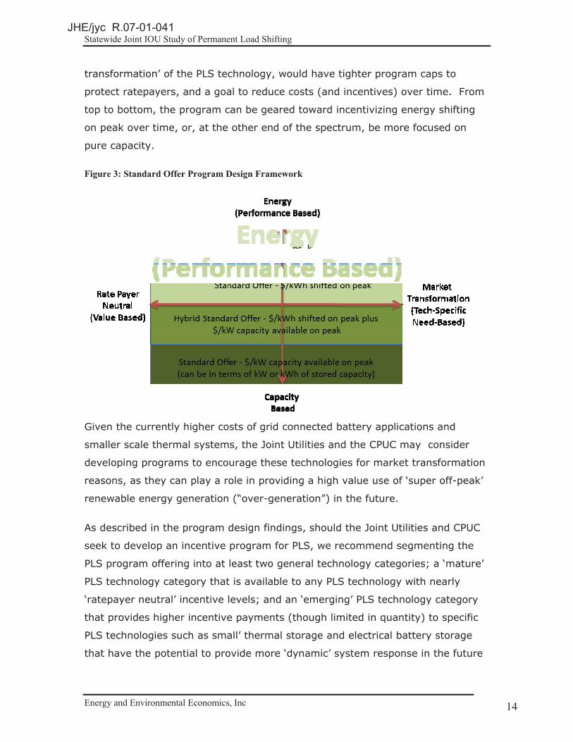
transformation’ of the PLS technology, would have tighter program caps to
protect ratepayers, and a goal to reduce costs (and incentives) over time. From
top to bottom, the program can be geared toward incentivizing energy shifting
on peak over time, or, at the other end of the spectrum, be more focused on
pure capacity.
Figure 3: Standard Offer Program Design Framework
Given the currently higher costs of grid connected battery applications and
smaller scale thermal systems, the Joint Utilities and the CPUC may consider
developing programs to encourage these technologies for market transformation
reasons, as they can play a role in providing a high value use of ‘super off-peak’
renewable energy generation (“over-generation”) in the future.
As described in the program design findings, should the Joint Utilities and CPUC
seek to develop an incentive program for PLS, we recommend segmenting the
PLS program offering into at least two general technology categories; a ‘mature’
PLS technology category that is available to any PLS technology with nearly
‘ratepayer neutral’ incentive levels; and an ‘emerging’ PLS technology category
that provides higher incentive payments (though limited in quantity) to specific
PLS technologies such as small’ thermal storage and electrical battery storage
that have the potential to provide more ‘dynamic’ system response in the future
JHE/jyc R.07-01-041

Statewide Joint IOU Study of Permanent Load Shifting
Energy and Environmental Economics, Inc Page 15 15
suitable to support renewable integration. We recommend that process shifting
be further evaluated to determine appropriate industries and loads to target for
program development.7
In addition, a number of best practices were observed from the pilots and other
PLS programs nationwide that are worth considering for California. The following
summary of the PLS program design recommendations should be considered:
� Divide PLS Program into at least two categories based on technology; one
for mature large scale PLS, and one for emerging PLS technologies, with
different program designs and goals.
o Mature: Large scale PLS deployment that minimizes ratepayer
incentives and provides thermal-based solutions
o Emerging: Market transformation for storage with focus on
integration with renewable resources and energy efficiency
� Program design should address each of the three stages of the PLS
system deployment through incentives, reports, or EM&V, to increase the
quality of the deployed PLS systems. These include;
o (1) feasibility and design of PLS systems,
o (2) quality control of construction and post-construction
performance testing, and
o (3) persistence of PLS operations.
� Provide consistent and predictable bill savings to encourage long term
customer investment in PLS technology, that
7 These program recommendations are based on our survey of best practices, utility pilot data
analysis, stakeholder interviews, cost-effectiveness results, and workshop discussion.
JHE/jyc R.07-01-041

Statewide Joint IOU Study of Permanent Load Shifting
Energy and Environmental Economics, Inc Page 16 16
o Provides a financeable level of long term rate stability to encourage
the initial capital outlay in a PLS system. This can be done with a
separate PLS rate, or by a ‘guarantee’ of minimum on- to off-peak
rate differentials or ‘grandfathering’ existing TOU rates
o Offers a ‘super’ off-peak rate to encourage charging after midnight
or 2am when the overgeneration problem is expected to be the
worst and energy has the lowest cost, and
� Encourage sustained PLS performance using performance-based
incentives and regular EM&V;
o Performance-based incentives could be achieved through one of
two approaches depending on technologies;
� A ‘PLS’ tariff with TOU rate differentials provides some
incentive to operate the PLS system well, and does not
require a specific baseline development. This approach is
more suitable for thermal storage.
� A standard offer model based on an energy payment ($/kWh
shifted) provides a direct performance-based incentive, but
would require strict guidelines for calculating baselines for
thermal or process shifting PLS technologies. Therefore, this
approach is easier to provide to electrical battery systems.
This approach also reduces potential for “gaming” with
battery systems (where batteries are used for non-PLS
purposes such as for providing uninterruptible power
supply).
o Both incentive approaches should be coupled with an EM&V
requirement to provide an ‘operations report’ and operational data
of the system and the whole customer load.
JHE/jyc R.07-01-041

Statewide Joint IOU Study of Permanent Load Shifting
Energy and Environmental Economics, Inc Page 17 17
o Incentives and incentive structure influence directly influence PLS
design and operations so it is important to provide incentives
consistent with program goals
o Simplicity and transparency of the performance metrics are critical
to minimizing program cost and encouraging customer adoption
As per the CPUC order that initiated this report, the Project Team has included a
detailed discussion of a PLS standard offer proposal that could apply generally to
any permanent load shifting technologies including, but not limited to, thermal
energy storage. The specifics of the Standard Offer are covered in detail in
Section 6 of this report.
JHE/jyc R.07-01-041

Statewide Joint IOU Study of Permanent Load Shifting
Energy and Environmental Economics, Inc Page 18 18
2. Introduction and Purpose of Study
2.1. Policy Background
2.1.1. CPUC Regulatory Background8
PLS has existed for many years as an electric customer demand side technology
that enables customers to reduce their energy bills by shifting loads from peak
periods, when rates are higher, to off-peak periods when rates are lower.
However, PLS has most recently been addressed in state regulatory policy
through the IOUs’ existing demand response programs.
In 2006, California experienced a severe heat storm that prompted the CPUC to
issue an Assigned Commissioner Ruling to augment the IOU’s recently approved
DR programs for 2007 and 2008, and to improve program performance with the
adoption of new programs and technologies. Workshops and discussions were
held on the performance of existing DR programs, and the recommendations to
improve and augment these programs were filed. Based on the
recommendations, the CPUC’s decision D.06-11-049 was issued in 2006 (“Order
Adopting Changes to 2007 Utility Demand Response Programs”) that advised the
IOUs on DR program improvements, as part of a broader effort to assure system
reliability and affordability.
Included in D.06-11-049 were a number of DR program modifications and
approval for new program designs for 2007 and beyond. While not specifically
considering PLS as energy efficiency or demand response, the CPUC determined
that load shifting from PLS may reduce the need for capacity investments,
reduce the likelihood of shortages during peak periods and lower system costs
overall by reducing the need for peaking units.
8 Information on the regulatory background were obtained through CPUC documents and discussion with the CPUC and IOU working group involved with this study.
JHE/jyc R.07-01-041

Statewide Joint IOU Study of Permanent Load Shifting
Energy and Environmental Economics, Inc Page 19 19
Numerous parties, including Ice Energy, consumer advocacy groups, and the
IOUs expressed their support for PLS programs using incentive funds from the
IOU’s DR programs. As a result, the CPUC ordered the IOUs to pursue RFPs and
bilateral arrangements for five year PLS projects from third parties that could be
implemented by the summer of 2007. The decision also allowed the IOUs to
allocate portions of their existing demand response budgets to offset the initial
installation costs of PLS technologies.9 In total, the decision allowed $24 million
of demand response budget to be shifted to PLS pilot projects ($10 million for
PG&E, $10 million for SCE and $4 million for SDG&E). The decision did not
specify a preference for any particular technology, but directed the utilities to
consider cost-effectiveness and other factors, such as ease of implementation.
The decision also specified that each utility was to file an advice letter with the
CPUC by February 28, 2007 that described the proposals chosen.
Subject to D. 06-11-049, each IOU issued an RFP for PLS pilot projects. After
proposals were solicited, each IOU evaluated their proposals using their own
criteria. Key evaluation criteria in PG&E’s RFP process included a benefit-cost
ratio, bidder’s track record and performance in load shifting programs, and the
methodology used to produce demand and energy savings. Key evaluation
criteria in SCE’s RFP process included cost, ease of implementation, the amount
of load shifting to be obtained by summer of 2008, potential for growth and
expansion, and reliability. Key evaluation criteria in SDG&E’s RFP process
included cost effectiveness, load growth potential, reliability, marketability, and
program’s ability to deliver energy savings with peak load shifting.
In accordance with D. 06-11-049, SCE and SDG&E filed advice letters with the
CPUC on February 28, 2007 that described the selected PLS proposals. PG&E
filed an advice letter on February 28, 2007 but were still in negotiations with PLS
vendors. On March 29, 2007 PG&E filed a supplemental advice letter that
described which the chosen PLS proposals. During this time, SCE filed an advice
letter recommending a non-thermal based PLS pilot program, which was rejected
9 The CPUC’s D.06-11-049 can be found here: http://docs.cpuc.ca.gov/word_pdf/FINAL_DECISION/62281.pdf .
JHE/jyc R.07-01-041

Statewide Joint IOU Study of Permanent Load Shifting
Energy and Environmental Economics, Inc Page 20 20
by the CPUC. A subsequent update of the advice letter incorporating three
different thermal based PLS technologies was later approved. Further details on
the PLS pilot are in Section 2.2.
During 2008, the IOUs filed applications for IOU specific DR program and budget
applications for approval of 2009-0211 DR programs. During the regulatory
process in which parties provide comments on the applications and during
evidentiary hearings, Transphase requested the CPUC to expand the existing PLS
program and to require utilities to create a PLS standard offer program that
could provide rebates up to $1,400 per installed kW of PLS over the 2009-2011
period. Ice Energy also encouraged the expansion of the PLS program within
IOUs demand response program applications. The IOUs proposed to continue the
existing pilot programs, as initially ordered through 2011, and not expand these
pilots beyond their authorized scopes.
CPUC responded in D.09-08-027, “Decision Adopting Demand Response
Activities and Budgets for 2009 through 2011”.10 The decision mandated the
IOUs to conduct a study (this study) to examine ways of expanding PLS; explore
a standard offer for PLS, including, but not limited to thermal energy storage;
consider ways to encourage PLS, such as through TOU rates or another RFP
process; summarize PLS offerings in the US; and evaluate an appropriate
incentive payment for a future standard offer. The findings of this report will
inform proposals to expand PLS in the IOU’s 2012-2014 demand response
applications, which are due by January 30, 2011.
The CPUC provided additional guidance in the “Administrative Law Judge’s Ruling
Providing Guidance for the 2012-2014 Demand Response Applications”.11 The
guidance includes clarification on the on the definition of PLS. The ruling states
that PLS involves shifting energy use from one time period to another on a
recurring basis and often involves storing electricity produced during off-peak
hours to use to support load during peak periods. Examples of PLS include
10 The CPUC decision D.09-08-027 can be found here: http://docs.cpuc.ca.gov/word_pdf/FINAL_DECISION/106008.pdf.11See http://docs.cpuc.ca.gov/efile/RULINGS/122575.pdf
JHE/jyc R.07-01-041

Statewide Joint IOU Study of Permanent Load Shifting
Energy and Environmental Economics, Inc Page 21 21
battery storage, thermal energy storage, and altering processes to shift the time
of use or order of production activities.
PLS as a demand side customer measure continues to be currently managed and
evaluated through the IOU’s demand response regulatory proceedings. In
October 2010 the CPUC stated in the proposed cost-effectiveness protocols for
demand response, “Decision Adopting a Method for Estimating the Cost-
Effectiveness of Demand Response Activities”, that it expected the demand
response cost-effectiveness protocols to apply to PLS projects, although the
CPUC may approve specific protocols for PLS in the future.12
2.1.2. Other Policy Background
In addition to the IOU’s PLS programs in the CPUC DR proceeding, there have
been policy initiatives by the CEC and CPUC to study energy storage and
enhancements to demand response that involve PLS. The CEC’s “Energy Storage
and Automated Demand Response Technologies to Support Renewable Energy
Integration” initiative aims to establish a technology baseline for its 2011
Integrated Energy Policy Report (2011 IEPR) and develop policies to accelerate
the deployment of energy storage and automated demand response
technologies. The CEC is also leading the development of a 2020 Energy Storage
Strategic Vision that will feed into the 2011 IEPR. The CPUC is required to
initiate a storage focused rulemaking pursuant to AB2514. That proceeding will,
by 2013, determine whether cost effective and technologically feasible energy
storage procurement targets should be established for 2015 and 2020. PLS
technologies are covered under both the CEC and CPUC initiatives.
2.2. PLS Pilots
2.2.1. SCE
Three PLS proposals were developed by the IOUs and approved by the CPUC in
SCE’s RFP process. They included Honeywell Utility Solutions administering an
12 The CPUC proposed decision can be found at: http://docs.cpuc.ca.gov/efile/PD/125044.pdf
JHE/jyc R.07-01-041

Statewide Joint IOU Study of Permanent Load Shifting
Energy and Environmental Economics, Inc Page 22 22
Ice Energy (packaged ice storage) program, ROI-CAC administering a chilled
water program, and Cypress Limited administering a CALMAC (packaged ice
bank) program. These three proposals provided marketing, installation,
commissioning and evaluation and measurement.
ROI-CAC enrolled four TES chilled water project customers at the beginning of
the program. These included three legacy thermal storage systems were
retrofitted and one new TES central plant was constructed. In each of the
retrofitted cases, the TES tanks were either partially used or undersized. The
modifications included chiller repiping, replacement, improved cooling towers,
controls and pumping.
The Honeywell program marketed Ice Energy’s Ice Bear technology which
required Honeywell to work with contractors, developers and city agencies. The
target customer size was 200-500 kW with a goal of subscribing 2,500 kW
shifted in total. To date, 2,205 kW have been reserved in applications to the
program with 142 kW in actual projects (21 Ice Bears). An incentive level of
$1,100/kW is being used and projects are now in measurement and verification
mode to demonstrate seasonal operations and shifting.
For the Cypress PLS program, a 5,000 kW program target was set with a
$250/kW customer incentive; 3,710 kW has been reserved to date with 2,449
kW completed. These projects tend to be larger community colleges.
2.2.2. PG&E
PG&E’s PLS program, “Shift & Save”, aims to promote TES. The program is
implemented by Cypress and Trane U.S. Inc. Both vendors have full
responsibility for the program and delivering the actual load shift results. The
total program shift goal is 7,950 kW and eligible customers are bundled service
commercial, industrial, agricultural, or large residential customers. Cypress
currently has a program goal of 6,750 kW subscribed under four customers with
JHE/jyc R.07-01-041

Statewide Joint IOU Study of Permanent Load Shifting
Energy and Environmental Economics, Inc Page 23 23
~ 125 kW installed to date.13 Among these, one is new, three are retrofit and all
use ice storage air conditioning. Trane U.S. Inc. has 1,200 kW subscribed with
three customers. Two of the installations are new and one is a retrofit and the
technologies include stratified chilled water and internal-melt-ice-on coil.
PG&E reviews the PLS program in three parts: (1) the project is evaluated for
participation, (2) the project is evaluated for an installation incentive and (3)
following the submission of EM&V reports at the end of the summer, the project
is evaluated for persistence payments.
2.2.3. SDG&E
SDG&E has two PLS programs: EPS’ refrigeration zone control module which
precools freezers, allowing them to operate without mechanical cooling during
peak periods and Cypress’ gas absorption and gas engine driven air conditioning
systems. The total program goal was 3,200 kW and to date, 2,900 kW has been
subscribed. The incentive levels for EPS are $150/kW. The incentives for
Cypress are $500/kW for systems greater than 100 tons and $700/kW for
smaller systems. These levels were based on bidders’ proposals.
2.3. Definition of PLS
The CPUC has defined PLS through regulatory orders and filings. In D.06-11-049
PLS is defined as “when a customer moves energy usage from one time period to
another on an ongoing basis.” The CPUC also does not consider PLS to be an
energy efficiency program because PLS does not always reduce energy
consumption; the CPUC does not consider PLS to be a demand response program
if it is not dispatchable or price responsive on a day-ahead or day-of basis.
For the purposes of this study, PLS is defined with the overarching goal of
“routine shifting from one time period to another during the course of a day to
help meet peak loads during periods when energy use is typically high and
13 Note, Cypress’s original goal was 2,700 kW from ice storage air conditioning but was recently increased to 6,750 kW, and expanded to include other technologies.
JHE/jyc R.07-01-041

Statewide Joint IOU Study of Permanent Load Shifting
Energy and Environmental Economics, Inc Page 24 24
improve grid operations in doing so (economics, efficiency, and/or reliability).”
This definition is guided by the principles of technology neutrality,
business/ownership neutrality, and the measurable shift at program level for
evaluation, measurement and verification.
The proposed definition is based on several elements: 1) permanent; 2) load
shifting; 3) location; and 4) additional value streams. By permanence, PLS must
provide a sustained capacity of load shifting in normal operation a large number
of days per year for many years. Through load shifting, PLS decreases usage
during peak hours and shifts loads to other hours to provide operational and
resource planning benefits for the utility or ISO systems (such as increasing load
to reduce ramp requirements). The location element requires the PLS technology
to be located behind an electricity customer’s meter, making all customer classes
eligible to participate. Finally, while PLS services are essential, additional value
streams should be provided if the PLS technology has the capability.
Table 3 shows the different applications and technology categories and provides
examples of each.
Table 3: PLS technology applications, categories and examples
Application Category Primary characteristics/ examples
Stationary Thermal storage Generate ice or chilled water at night, then use this stored ice or chilled water to provide cooling during the day.
Stationary Non-thermal storage
Chemical batteries, mechanical storage – e.g., fly wheels, modular compressed air (CAES)
Stationary Facility process shifting
Processes conducted within a facility that are shifted from one time period of the day to another
Mobile Plug-in electric vehicles
Not in scope (Because mobile storage has a concurrent proceeding at the CPUC)
The following elements are outside the scope of PLS. First, PLS is not solely
event-based demand response. While PLS does provide for shifting in normal
operations, it does not provide shifting in response to electrical grid emergencies
or constraints as event based demand response does. Second, PLS is not
behavior-based energy efficiency. PLS is provided and quantified by discrete
JHE/jyc R.07-01-041

Statewide Joint IOU Study of Permanent Load Shifting
Energy and Environmental Economics, Inc Page 25 25
equipment or controls, not solely by general customer behavior modification, and
it does not reduce the level of customer service. Third, the load reduction and
shifting that can be achieved by best practices commissioning, retro or
recommissioning, or adjustment of controls is not considered PLS, unless such
practices are being applied directly to existing legacy PLS technologies (such as
unused thermal storage tanks) and are not currently being implemented through
energy efficiency programs. Finally, fuel switching is not PLS.
JHE/jyc R.07-01-041

Statewide Joint IOU Study of Permanent Load Shifting
Energy and Environmental Economics, Inc Page 26 26
3. Study Methodology
The PLS cost-effectiveness evaluation is performed using two models. The first
model, the PLS Cost-effectiveness Tool (PLS CE Tool), is designed to assess a
wide variety of technologies and scenarios, and overall PLS program cost-
effectiveness. It uses publicly available and stakeholder provided data, in a
transparent model to calculate the cost-effectiveness of a PLS technology or
program. The PLS CE Tool is implemented in Analytica and can be downloaded
and run using the free Analytica Player, and modified using the Analytica
platform.14 With the tool, the balance between customer incentives and the
impact on non-participating ratepayers is evaluated. Using 8,760 hourly PLS
system impacts, customer loads, retail rates and avoided costs, the tool
calculates the net present value of the costs and benefits over the life of PLS
technology. With the Analytica Free Player, stakeholders can view and audit the
calculations, as well as see how the cost-effectiveness results would change for
the 15 California IOU tariffs modeled.
A more detailed financial pro-forma model, developed by StrateGen, provides a
more in-depth analysis of cost-effectiveness from the participating customer
perspective. This model analyzes specific customer scenarios with customer
specific financial information. Much of the data required for an analysis of this
depth is held as proprietary for the customer or technology provider and this
model is not available for public review.
14 Available for download from Lumina Decision Systems, Inc. at http://www.lumina.com/ana/player.htm
JHE/jyc R.07-01-041

Statewide Joint IOU Study of Permanent Load Shifting
Energy and Environmental Economics, Inc Page 27 27
• Public and transparent
• Avoided cost calculations using public data
• Public cost estimates and those provided through public stakeholder process
• Cost test results at program level
• Evaluate trade-offs between customer, utility and non-participating ratepayer costs and benefits
E3 PLS Cost-effectiveness Tool• Proprietary tool (inputs &
outputs provided publicly)
• Financial Proforma with cash flow
• Participant perspective
• Supports evaluation of incentives and rate design to encourage adoption
StrateGen Proforma
Ratepayer Perspective Industry Perspective
Figure 4: Summary of the E3 PLS Cost-effectiveness Tool and the StrateGen Proforma model.
3.1. Cost effectiveness
3.1.1. PLS Modeling Inputs
Four broad input categories are required for PLS cost-effectiveness evaluation:
PLS system costs, PLS system performance and load impacts, retail customer
rates, and avoided costs. These are described below.
3.1.1.1. PLS System Costs
PLS system costs were gathered from utility program managers and from
technology vendors. The PLS CE Tool uses representative estimates of system
costs for the range of available technologies, and program level costs where
available. Where necessary, we worked with customers and technology vendors
to produce more detailed cost estimates.
3.1.1.2. PLS System Performance
The utilities and technology community provided the project team with data on
system performance. The data provided varied substantially in terms of
JHE/jyc R.07-01-041

Statewide Joint IOU Study of Permanent Load Shifting
Energy and Environmental Economics, Inc Page 28 28
temporal duration, interval, and baseline information. The project team worked
closely with the utilities and vendors to construct 8,760 hourly profiles of PLS kW
impacts. These impacts are used to estimate the customer bill savings and the
avoided cost benefits over the life of the PLS technology. Where available, the
customer’s end-use load profile was used in combination with the PLS system
impacts to calculate a before and after load shape. In other cases, end-use load
data was not available and the PLS impact alone was used. End-use load data is
most important for evaluating demand charge bill savings, but not necessary for
evaluating bill savings from energy charges and avoided cost benefits. As several
stakeholders have noted, it is important that the hourly input data (load impacts
and avoided costs) be in alignment to provide meaningful results.
3.1.1.3. Retail Tariffs
Recent tariffs were gathered from the IOU websites for the residential,
commercial and industrial classes. A full range of demand charges, TOU rate
differentials and dynamic rates were included for all three utilities. The rates are
entered into both models, each of which calculates the rate applicable for each
hour in each month based on the tariff rules. With this disaggregated rate data,
the models calculate the change in the customer bills realized with PLS.
3.1.1.4. Avoided Costs
Avoided cost benefits provided by PLS and other Distributed Energy Resources
(DER) include seven categories: generation energy, losses, ancillary services,
system (generation) capacity, T&D capacity, environmental costs, and avoided
renewable purchases. In addition to these benefit categories, we also
investigated the renewable integration benefits of load following and
overgeneration that could be provided by PLS.
The avoided costs used for this analysis are derived from the Distributed
Generation (DG) Cost-Effectiveness framework adopted by the CPUC in
D. 09-08-026, which specifies the use of a marginal avoided cost-based
approach to distributed resource valuation. The avoided costs are calculated
using the Avoided Cost Calculator with some modifications. The Avoided Cost
JHE/jyc R.07-01-041
Statewide Joint IOU Study of Permanent Load Shifting
Energy and Environmental Economics, Inc Page 29 29
Calculator draws heavily on the methods established by other CPUC cost-
effectiveness assessments for distributed resources including distributed
generation (DG), demand response (DR), and energy efficiency (EE). More
information about the calculation of avoided costs is found in Appendix A.
3.1.1.5. Modeling Approach
Both the PLS CE Tool and the StrateGen Proforma model compare the cost of
installing and operating the PLS system with the benefits generated over the life
of the system. The PLS CE Tool uses system costs expressed in $/kW installed
and annual O&M costs expressed in $/kW-Yr. For the StrateGen Proforma Model
more detailed customer specific cost and financing inputs are used.
The PLS system impacts are estimated on an 8,760 hourly basis and the avoided
cost components are also calculated on an 8,760 basis. In the case of
generation and T&D capacity, the benefit values (in $/kW-Yr.) allocated to
specific hours (in $/MWh) are based on system load and temperature data
respectively. Retail rate impacts are also calculated on an hourly basis for
energy charges and a monthly basis for demand charges.
The models compute the present value of the system installation and operating
cost and compare those against the present value of the applicable benefits for
each cost-effectiveness test.
3.1.2. Cost-effectiveness Tests
The cost-effectiveness of individual technologies and overall utility PLS program
offerings are evaluated. These tests are described in the California Standard
Practice Manual for the Economic Analysis of Demand-Side Programs and
Projects, commonly referred to as the Standard Practice Manual (SPM), issued by
the California Energy Commission (CEC) and the California Public Utilities
Commission (CPUC) in 2001. The four cost-effectiveness tests performed for
this analysis are summarized in Table 4 and described below.
JHE/jyc R.07-01-041

Statewide Joint IOU Study of Permanent Load Shifting
Energy and Environmental Economics, Inc Page 30 30
Table 4. Cost effectiveness tests applied in scenario analysis tool
3.1.2.1. Total Resource Cost-effectiveness Test (TRC)
The TRC is the primary test used to evaluate the overall cost-effectiveness of
DERs in California and many other jurisdictions. It measures the net benefits to
the region as a whole, irrespective of who bears the costs and receives the
benefits. Unlike the other cost tests, the TRC does not take the view of any
particular stakeholder. The incremental costs of purchasing and installing the
PLS system above the cost of standard equipment that would otherwise be
installed, and the overhead costs of running the PLS program are considered.
The avoided costs are the benefits. Bill savings and incentive payments are not
included, as they yield an intra-regional transfer of zero (‘benefits’ to customers
and ‘costs’ to the utility that cancel each other on a regional level).
The TRC does not evaluate distributional impacts among stakeholders. The other
three tests are distributional tests that evaluate the net benefits to different
stakeholders. These include non-participating ratepayers (RIM), the utility or
program administrator (PAC) and the participant (PCT).
3.1.2.2. Ratepayer Impact Measure
The Ratepayer Impact Measure (RIM) examines the impact of the program on
non-participating customers through changes in utility rates. The RIM test is
used to define the ‘ratepayer neutral’ incentive level. Most DERs that provide
Cost Test Acronym Purpose
Total Resource Cost Test TRC Financial impact from a societal level is used to determine whether the program should be offered. Incentive levels do not change the TRC result.
Ratepayer Impact Measure
RIM Impact on non-participating ratepayers is used to balance the incentives so that other ratepayers are not disproportionately impacted by the program
Program Administer Cost PAC Input on ratepayers overall is used to estimate the total costs of the program net of system benefits
Participant Cost Test PCT Financial proposition to the customer is used to define incentive and shows relative attractiveness of the program and estimating participation
JHE/jyc R.07-01-041

Statewide Joint IOU Study of Permanent Load Shifting
Energy and Environmental Economics, Inc Page 31 31
energy efficiency put upward pressure on retail rates as the remaining fixed
costs are spread over fewer kWh and do not ‘pass’ the RIM test. In the case of
PLS, energy sales are shifted from higher cost on-peak periods to lower cost off-
peak periods. This can reduce utility revenues and put upward pressure on
utility rates if the total bill savings is less than the savings in utility avoided cost.
The costs included in the RIM test are program overhead and incentive payments
and the cost of lost revenues due to reduced sales. The benefits included in the
RIM test are the avoided costs of energy saved through the efficiency measure
(same as the TRC).
3.1.2.3. Program Administrator Cost-effectiveness Test
The Utility/Program Administrator Cost Test (PAC) examines the costs and
benefits of the program from the perspective of the entity implementing the
program (utility, government agency, non-profit, or other third-party).15 The
costs included in the PAC are overhead and incentive costs. Incentive costs are
payments made to the customers to offset purchase or installations costs. The
PAC does not include bill reductions. The benefits are equal to the lifecycle utility
avoided costs.
3.1.2.4. Participant Cost-effectiveness Test
The Participant Cost Test (PCT) examines the costs and benefits from the
perspective of the customer installing the PLS system. Costs include the
incremental costs of purchasing and installing the PLS system above the cost of
standard equipment that would otherwise be purchased by the customer. The
benefits include bill savings realized to the customer through reduced energy
consumption and the incentives received by the customer and any applicable
government tax credits or incentives.
15 The UCT/PAC was originally named the Utility Cost Test. As programs management has expanded to government agencies, not-for-profit groups and other parties, the term “Program Administrator Cost Test” has come into use, however the computations are the same. This document refers to the UCT/PAC as PAC for simplicity.
JHE/jyc R.07-01-041

Statewide Joint IOU Study of Permanent Load Shifting
Energy and Environmental Economics, Inc Page 32 32
3.1.2.5. Cost-effectiveness Test Summary
The primary cost and benefit categories for each test are shown in Table 5. The
TRC, RIM and PAC all include the same avoided costs as benefits to the region
(in the case of the TRC) and to the utility (in the case of the RIM and PAC).
Expressing the regional perspective, the TRC does not include incentive
payments or bill savings, which are intra-regional transfers.
The RIM includes all costs that must be borne by non-participating ratepayers,
including program overhead and incentives, which are additional expenditures
incurred by the utility that increase the total revenue that the utility must collect.
The RIM includes bill reductions as revenue losses, which increases the amount
of revenue that must be collected from other customers, putting upward
pressure on rates. The PAC looks at the utility revenue requirement only,
including program overhead and incentive payments as costs. Note that the
system cost is not included.
Finally, the PCT looks at the customer perspective. The benefits to the customer
are the bill savings and incentives. These benefits are weighed against the cost
to the customer of installing and operating the PLS system.
Table 5: Costs and Benefits Included in Each Cost-effectiveness Test
Component TRC RIM PAC PCT
Avoided Cost Benefits Benefit Benefit Benefit -
Equipment and install costs Cost - - Cost
Program overhead costs Cost Cost Cost -
Incentive payments - Cost Cost Benefit
Bill Savings - Cost - Benefit
3.1.3. PLS Avoided Cost Benefits
Avoided cost benefits provided by PLS (and DERs in general) include seven
categories: Generation Energy, Losses, Ancillary Services, System (Generation)
Capacity, T&D Capacity, Environmental costs, and Avoided Renewable
Purchases. The value is calculated as the sum in each hour of the seven
JHE/jyc R.07-01-041

Statewide Joint IOU Study of Permanent Load Shifting
Energy and Environmental Economics, Inc Page 33 33
individual components. A more detailed description of each of the components is
provided in Table 6.
Table 6: Components of marginal energy cost
Component Description
Generation Energy Estimate of hourly wholesale value of energy adjusted for losses between the point of the wholesale transaction and the point of delivery
System Capacity The costs of building new generation capacity to meet system peak loads
Ancillary Services The marginal costs of providing system operations and reserves for electricity grid reliability
T&D Capacity The costs of expanding transmission and distribution capacity to meet peak loads
Environment The cost of carbon dioxide emissions associated with the marginal generating resource
Avoided RPS The avoided net cost of procuring renewable resources to meet an RPS Portfolio due to a reduction in retail loads
Figure 5 shows a three-day snapshot of the avoided costs, broken out by
component, for Climate Zone 13. As shown, the cost of providing an additional
unit of electricity is significantly higher in the summer afternoons than in the
very early morning hours. This chart also shows the relative magnitude of
different components in this region in the summer for these days. The highest
peaks of total cost shown in Figure 5 of almost $1,000/MWh in a few hours are
driven primarily by the allocation of generation and T&D capacity to the highest
load hours, but also by higher wholesale energy prices during the middle of the
day.
JHE/jyc R.07-01-041

Statewide Joint IOU Study of Permanent Load Shifting
Energy and Environmental Economics, Inc Page 34 34
Figure 5: Three-day snapshot of energy values in CZ2
�
$0
$200
$400
$600
$800
$1,000
$1,200
$1,400
$1,600
Thu,�Aug13
Fri,�Aug�14 Sat,�Aug�15
Avoi
ded�
Cost
�($/M
Wh) T&D
Capacity
Emissions
Ancillary�Services
Losses
Avoided�RPS
Energy
3.1.3.1. Generation Energy
The avoided cost of energy reflects the marginal cost of generation needed to
meet load in each hour. In the near term (2010-2014), the value of energy is
based on forwards for NP15 and SP15. In the long run, the avoided cost of
energy is calculated based on an MPR-style gas price forecast and an assumption
that market heat rates will remain flat beyond 2014. The hourly shape of the
value of energy is based on historical day-ahead LMPs at the PG&E and SCE load
aggregation points—these historical data sets are used to adjust the annual
averages to obtain an hourly shape in each year. The hourly shaped values of
energy are further adjusted by losses factors that capture the lost energy
between the point of wholesale transaction and the point of delivery. These
factors vary by time-of-use period and are specific to each utility.
3.1.3.2. Generation Capacity
The generation capacity value captures the reliability-related cost of maintaining
a generator fleet with enough nameplate capacity to meet each year’s peak
loads. With the current surplus of capacity on the CAISO system—expected
reserve margins for the summer of 2010 are in the range of 30-40%—the
current value of capacity is low. The avoided cost of capacity transitions to a
long-run value based on the cost of new entry for a new combustion turbine in
JHE/jyc R.07-01-041

Statewide Joint IOU Study of Permanent Load Shifting
Energy and Environmental Economics, Inc Page 35 35
2015 and is calculated for each year thereafter. As with energy, the value of
capacity is adjusted upwards for peak period losses on the wholesale system.
The value of capacity is further scaled up by 15% to capture the value associated
with a permanent load shift off peak. As demand-side resources, PLS resources
reduce peak loads and planning reserves requirements such that the shift of a
single kilowatt off peak results in a reduction in net supply requirements of 1.15
kW.
The residual capacity value in each year is allocated to the top 250 CAISO
system load hours. The top 250 hours are selected based on the system loads
over the four years from 2006 to 2009. In comments regarding the DR Cost-
effectiveness Protocols parties have argued that this methodology
inappropriately limits the allocation of capacity value to July, August and
September. An alternative method averaging four years of historical data, rather
than just one, provides a wider allocation of value that also includes May and
June. Because the PLS technologies evaluated provide equal or higher impacts
in the Summer months, the allocation of capacity value does not have an
appreciable effect on the cost-effectiveness results. The Avoided Cost Model,
however, may be updated in the DR or other proceeding to update the allocation
of capacity value.
3.1.3.3. Ancillary Services (A/S)
The reduction in the procurement of spinning and non-spinning reserves is
included as a benefit stream in the avoided costs. The Avoided Cost Calculator
assumes that the value of spinning reserves in each hour is equal to 1.0% of the
value of energy in that hour.
3.1.3.4. T&D Capacity
The avoided costs include the value of the potential deferral of transmission and
distribution network upgrades that could result from reductions in local peak
loads. Through an analysis of general rate cases, E3 has gathered utility-specific
data on the value of transmission and distribution system deferrals on growth-
related infrastructure. The network constraints of a distribution system must be
JHE/jyc R.07-01-041

Statewide Joint IOU Study of Permanent Load Shifting
Energy and Environmental Economics, Inc Page 36 36
satisfactory to accommodate the area’s local peaks; accordingly, the DG Cost-
effectiveness Framework allocates the deferral value in each climate zone to the
hours of the year during which the system is most likely to be constrained and
require upgrades—the hours of highest local load. Because local loads were not
readily available for this analysis, hourly temperatures were used as a proxy to
develop allocation factors for T&D value.
3.1.3.5. Environment
Reductions in load also reduce emissions of greenhouse gases. While the future
of carbon pricing is uncertain, E3 has included it as a benefit, using the Synapse
Mid-Level forecast of carbon prices specifically designed for integrated resource
planning in the electricity sector. Hourly emissions rates are calculated based on
the hourly market prices, from which the implied heat rate of the marginal
generator is calculated.
3.1.3.6. Avoided Renewable Purchases
Because of California's commitment to reach an RPS portfolio of 33% of total
retail sales by 2020, any reductions to total retail sales will result in an additional
benefit by reducing the required procurement of renewable energy to achieve
RPS compliance. This benefit is captured in the avoided costs through the RPS
Adder. The RPS adder is calculated by subtracting the expected energy, capacity,
and emissions values from the levelized busbar cost of a marginal potential wind
farm in California. Because this adder is flat in all hours, it has a relatively
minimal effect on the valuation of most PLS systems, which do not result in
substantial net reductions in retail sales.
3.1.3.7. Load Following
Load following refers to the capability to manage the difference between 20
minute ramps and 5 minute energy schedules set by the CAISO. Load following
is one of two additional avoided cost benefits considered specifically for PLS.
While not a discrete service or market product currently, load following has been
identified as a key requirement for integrating increasing penetration of
JHE/jyc R.07-01-041

Statewide Joint IOU Study of Permanent Load Shifting
Energy and Environmental Economics, Inc Page 37 37
intermittent renewable resources. By increasing Off-Peak load and reducing On-
Peak load, PLS would appear to have the potential to reduce load following
requirements, particularly in the morning and evening ramp periods. The CAISO
20% RPS Study, however, shows that the primary driver of load following
requirements is not forecasted load, but instead load and intermittent generation
forecast error. Fixed PLS would therefore not appreciably reduce load following
requirements. Technologies that are dispatchable with notification times of 20
minutes or less could potentially provide load following services in the future.
3.1.3.8. Overgeneration
Overgeneration is excess generation that must be curtailed or spilled when load
is below minimum generation from base load, hydro and must take resources.
As increasing penetration of wind and solar resources are added to the grid, the
number of hours during which generation exceeds net loads will increase.
Overgeneration is driven primarily by intermittent wind, which has higher
generation during off-peak hours when loads are the lowest. With anticipated
wind generation of ~2,500 MW in 2010, overgeneration does not appear to be an
issue. However, by 2020, installed wind capacity may reach ~9,000 MW.
Modeling performed by E3 suggests this would lead to ~1,700 hours of
overgeneration, predominately in Spring, when hydro generation is high and
loads are moderate. The PLS CE Tool includes the expected hours in which
overgeneration is most likely to occur in each year based on the expected level
of wind penetration.
Curtailing wind generation would impose a cost on the utility in terms of lost RPS
qualifying generation. For each MW of wind curtailed, an additional MW of RPS
qualifying generation must be purchased. The estimated cost of marginal
renewable generation each year is included as an avoided cost benefit, starting
about ~$90/MWh in 2008.
3.1.4. Key Sensitivities
There are two aspects of the PLS modeling that may significantly impact the
cost-effectiveness results: the use of short-run vs. long-run generation capacity
JHE/jyc R.07-01-041

Statewide Joint IOU Study of Permanent Load Shifting
Energy and Environmental Economics, Inc Page 38 38
value, and aligning PLS system impacts with the allocation of generation capacity
and T&D capacity value to individual hours. The general scenario modeling
(Section 4.1.3) results explore sensitivity to the short-run vs. long-run
generation capacity. The sensitivity to capacity value is explored with the case
studies (Sections 4.1.4 and 4.1.5).
3.1.4.1. Short vs. Long-run Capacity Value
The forecast of generation capacity value includes both a short-run and a long-
run component; the transition point between the two occurs in the resource
balance year. The short-run value of capacity is based on the 2008 resource
adequacy value of $28/kW-Yr. — the relatively low value reflects the large
surplus of capacity currently available on the CAISO system. Capacity value in
the years between 2008 and resource balance is calculated by linear
interpolation. Beginning in the resource balance year, the value of capacity is
calculated based on the cost of a simple-cycle combustion turbine (CT), as that
is the first year in which new capacity resources may be needed to meet the
growth of peak loads and reliability requirements. The long-run capacity value is
equal to the CT’s annualized fixed cost, less the net revenues it would earn
through participation in the real-time energy and ancillary services markets—this
figure is the “capacity residual.” This long-term capacity value is closer to
$100/kW-Yr or more in most studies of residual capacity value or Cost of New
Entry (CONE).
The use of short- vs. long-run values for generation capacity has a substantial
impact on the cost-effectiveness of DR and PLS. There are two schools of
thought regarding whether the short- or long-run generation capacity value is
the most appropriate for valuing DERs. Ratepayer advocates argue that in a
market with excess capacity, the lower, short-run value best expresses the
actual capacity costs avoided and therefore the economic benefits realized by
utility ratepayers and the region as a whole. Others argue that relying on short-
run values does not appropriately reflect the position of energy efficiency and
demand response at the top of the loading order. In addition, parties argue that
with a planning reserve margin the condition of sufficient or excess capacity will
JHE/jyc R.07-01-041

Statewide Joint IOU Study of Permanent Load Shifting
Energy and Environmental Economics, Inc Page 39 39
persist indefinitely, preventing EE or DR from ever receiving the higher, long-
term capacity value that is typically used when evaluating investments in
traditional generation capacity. The use of a long-term capacity value
throughout the period of analysis is done in the sensitivity analysis.
3.1.4.2. Aligning PLS Impacts with Load, Weather and Prices
PLS impacts were gathered from case studies, sometimes, spanning different
time periods. The generation and T&D capacity values are, on the other hand,
allocated to individual hours based on system load from 2006 to 2010 and
temperature data from July 2009 to June 2010, respectively. This period was
used to incorporate a full year of MRTU market while excluding the three months
immediately after MRTU start-up in April 2010 while implementation issues were
worked through. Therefore, for some case studies or impact estimates, impacts
that may vary due to temperature will not line up exactly with the 2009-2010
load or temperature data. This discrepancy may affect estimates of demand
charge reductions, which are based on the coincidence of the system impacts
with customer load, and may also be weather dependent.
Sensitivities are performed (Sections 4.1.4 and 4.1.5) to account for the
possibility that the cost-effectiveness modeling does not fully capture the
capacity value of some PLS systems, due to misalignment with PLS data.
3.1.5. Broad Scenario Analysis (“Matrix”)
A broad scenario analysis was conducted to evaluate the avoided costs and bill
savings of PLS over a range of hypothetical conditions. The broad scenario
analysis is based on generic, idealized, shift profiles without specific technology
performance data. This approach allows for exploring the idealized value of load
shifting, independent of any specific PLS technology performance or
environmental factors.
The assumed shift is constant, occurs every day of the year, and is flat over the
duration of the discharge. For each sensitivity in the broad scenario analysis
(e.g., for a specified climate zone and round-trip efficiency), there are 66 shift
JHE/jyc R.07-01-041

Statewide Joint IOU Study of Permanent Load Shifting
Energy and Environmental Economics, Inc Page 40 40
profiles. Each of the 66 profiles is defined by the shift start hour (each hour
between 7 am and 5 pm) and the shift duration (1, 2, 4, 6, 8 and 10 hours). For
each profile, the shift occurs every day of the year. There are a total of 66
combinations of shift profiles based on a shift start hour ranging from 8 am to 6
pm and discharge duration of 1, 2, 4, 6, 8 and 10 hours.
Figure 6 illustrates the before and after load profiles for one day of the shift
profile with a shift start hour of 13 and a duration of 4 hours. This shift
discharges a constant output from 1 PM until 5 PM every day of the year.
Figure 6: One Day of a Shift Profile with 4 Hour Duration and Shift Start at 1 PM
0
50
100
150
200
250
300
350
400
Load
�(kW
) BaselineLoadProfile
After�ShiftLoadProfile
3.1.5.1. Generic Benefit Matrix Assumptions
Round-trip efficiency: Round-trip efficiency is defined as the fraction of energy
discharged, relative to the energy required for charging. If the PLS device is
assumed to have 100% round-trip efficiency, the shifted profile will consume the
same amount of energy relative to the baseline profile. Some PLS devices, such
as batteries, will have a round-trip efficiency of less than 100%. Other PLS
devices, such as some thermal storage units, may show an energy efficiency
improvement relative to the baseline cooling unit and show a “round-trip”
efficiency greater than 100%.
JHE/jyc R.07-01-041

Statewide Joint IOU Study of Permanent Load Shifting
Energy and Environmental Economics, Inc Page 41 41
In developing the Matrix avoided costs, the hypothetical PLS device is initially
assumed to have 100% round-trip efficiency. Sensitivities were separately
conducted for 80% and 120% round-trip efficiencies.
Baseline profile: The baseline profile for all the broad scenario analysis
examples is the California Commercial End-Use Survey (CEUS) “All Commercial”
load profile, normalized to a peak load of 500 kW. The baseline profile does not
impact the avoided cost calculations in any way, since the avoided costs are
dependent only on the difference between the baseline and shifted profile). The
baseline profile does, however, impact bill savings.
Charging sequence: For the broad scenario analysis, we assume the PLS
device is not able to charge faster than it can discharge, so charge kW is set
equal to the peak capacity reduction. For a 100% efficient PLS device the
number of charging hours will equal the number of discharging hours. An
inefficient device will have more charge hours than discharge hours.
Each of the 66 shifts is assigned a least cost charge start hour that minimizes
the avoided cost penalties from charging. For example, for the 4 hour discharge
in Figure 6, the charge start and duration are 1 AM and 4 hours. We determine
least cost charge start hour for each of the 66 shift profiles based on the average
avoided costs from all climate zones. For each shift profile, the discharge hours
are considered unavailable for charging, and then the minimum charge period of
the required duration is selected.
Bill Impacts: Hypothetical bill impacts were estimated to conduct a RIM test for
the broad scenario analysis. A generic rate with both TOU energy charges and an
on-peak demand charge was defined. The generic rate is roughly an “average”
of all the IOUs general service tariffs and does not represent a specific rate. In
summer, the on-peak energy charge is $0.20/kWh and the off-peak charge is
$0.10/kWh. In winter, the on-peak energy charge is $0.12/kWh and the off-
peak energy charge is $0.09/kWh. The peak period throughout the year is
Monday-Friday, 12-6 PM, excluding holidays. The on-peak demand charge is
$10/kW year round.
JHE/jyc R.07-01-041

Statewide Joint IOU Study of Permanent Load Shifting
Energy and Environmental Economics, Inc Page 42 42
3.1.6. Cost effectiveness of individual cases
The cost-effectiveness of specific PLS cases were estimated to benchmark
against the results of the broad scenario analysis. The cost-effectiveness tests
applied are the TRC, participant, and ratepayer impact (RIM) tests. To review,
the TRC test evaluates the cost-effectiveness of the example installation to
society as a whole. The participant cost test evaluates the cost-effectiveness of
the PLS installation from the perspective of the technology owner. The RIM test
evaluates the cost-effectiveness of the PLS installation from the perspective of a
non-participant ratepayer.
Figure 7: Cost-effectiveness Evaluation
Energy
A/S
RPS�AdderTOU�Energy
Charge�Benefits
Capacity
T&D
DemandCharge
BenefitsWind�
Overgen
IncrementalPLS�System
Costs
$0
$500
$1,000
$1,500
$2,000
$2,500
Pres
ent�V
alue
�$/k
W�c
usto
mer
�pea
k�re
duct
ion
Participant results before incentive
Ratepayer Impact before incentive
TRC test without program admin
Figure 7 illustrates an example result of the cost-effectiveness tests. In this
example, the participant requires a ~ $400/kW incentive to break even on the
PLS technology cost, on a lifecycle basis. The ratepayer impact test shows that
non-participant rate-payers will transfer ~ $300/kW to PLS participants without
an incentive or ~ $700/kW with an incentive. The TRC is negative by
~ $800/kW (excluding program administration).
JHE/jyc R.07-01-041

Statewide Joint IOU Study of Permanent Load Shifting
Energy and Environmental Economics, Inc Page 43 43
3.1.7. Specific Case Studies: Simulated Installations
The broad scenario modeling estimates the “idealized” value of shifting (an upper
bound) for a range of hypothetical shift scenarios, independent of the PLS
technology employed. To explore the value of more realistic PLS scenarios,
simulated scenarios of chilled water and battery technologies were evaluated.
Simulated Stratified Chilled Water Scenarios: A set of eight partial-shift
(50%) chilled water scenarios, generated by the Energy Pro building energy
simulation software, were evaluated. The modeled outputs were provided by
PG&E and were developed for PG&E by Green Building Studio to inform PG&E’s
evaluation of their Permanent Load Shift program16. Two different building types
(office and retail) in four different climate zones (3, 4, 12 and 13) were
evaluated. For each of the eight combinations, a baseline and TES scenario were
generated. The baseline system has an HVAC system and building design that
meets Title 24 energy code requirements. The TES scenario incorporates a
chilled water tank that is designed to offset 50% of the peak load.
The TES tank size for the different scenarios ranges from ~ 350 to 700 ton-
hours. The TES is used as the primary cooling source from 12-6pm, provides
supplemental cooling from 8am-12 pm, with remaining capacity discharged from
6 pm – 10 pm. The TES is recharged from 10 pm – 6 am. The chillers and TES
are unused on holidays and weekends.
Rough costs of the TES system are estimated using the TES capacity (in ton-
hours) and applying a range of $150/ton-hr - $400/ton-hr. These values were
selected based on information provided by stakeholders, where the range is due
to differences in level of engineering, material of the tank, and whether the tank
is below or above ground. Smaller chilled water systems tend to be more
expensive, on a unit basis, compared to larger systems. It is worth noting that
an ice storage system may be more typically applied over chilled water for a
system this size. However, the cost of such a system is expected to be within the
16 Cristofani, M., Debacker, S. B., Welland, J., Pacific Gas and Electric, Evaluation of Load Impacts of the Pacific Gas and Electric Company Permanent Load Shift Program. April 2010.
JHE/jyc R.07-01-041

Statewide Joint IOU Study of Permanent Load Shifting
Energy and Environmental Economics, Inc Page 44 44
range selected here (The profiles for ice storage, however, will be different from
the chilled water profiles).
Simulated Battery Scenarios: Two battery technologies were also simulated
for the analysis. The first battery technology is a bipolar lead-acid battery with
performance and cost data supplied by the manufacturer, AIC/East Penn. The
second battery technology is a vanadium redux flow battery with performance
and cost data supplied by the manufacturer, Prudent. While several other battery
technologies do exist and are commercially available, these two technologies
were the only battery specifications supplied by stakeholders with enough data
to support the required analysis.
The battery sizes were selected based on the case study loads available and the
availability of battery size data from the manufacturer to optimize the kW
capacity and kWh duration. Load data utilized included two different
manufacturing facilities in Southern California. The bipolar lead-acid battery is
priced the same on a kWh capacity rating for 100kW sizes or greater (i.e. a
100kW, 200kWh system would be priced the same on a $/kWh basis as a
100kW, 800kWh system). The vanadium redux flow battery data only allowed for
one size system to be selected to optimize for the case study load profiles—a
200kW, 800kWh system size. The primary reason for the differences between
these battery costing metrics was the lack of detailed data for multiple vanadium
redux flow battery kWh duration and kW capacity specifications.
Given the relative flexibility in operational dispatch of battery energy storage,
including the two battery technologies modeled in this study, several sensitivities
were conducted around these batteries and include the following:
� Simple daily permanent load shifting every weekday of the year
� Dynamic dispatchable load leveling every weekday of the year
JHE/jyc R.07-01-041
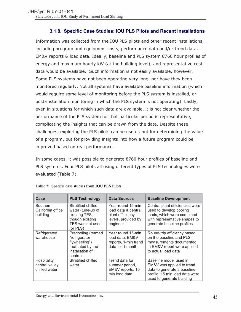
Statewide Joint IOU Study of Permanent Load Shifting
Energy and Environmental Economics, Inc Page 45 45
3.1.8. Specific Case Studies: IOU PLS Pilots and Recent Installations
Information was collected from the IOU PLS pilots and other recent installations,
including program and equipment costs, performance data and/or trend data,
EM&V reports & load data. Ideally, baseline and PLS system 8760 hour profiles of
energy and maximum hourly kW (at the building level), and representative cost
data would be available. Such information is not easily available, however.
Some PLS systems have not been operating very long, nor have they been
monitored regularly. Not all systems have available baseline information (which
would require some level of monitoring before the PLS system is installed, or
post-installation monitoring in which the PLS system is not operating). Lastly,
even in situations for which such data are available, it is not clear whether the
performance of the PLS system for that particular period is representative,
complicating the insights that can be drawn from the data. Despite these
challenges, exploring the PLS pilots can be useful, not for determining the value
of a program, but for providing insights into how a future program could be
improved based on real performance.
In some cases, it was possible to generate 8760 hour profiles of baseline and
PLS systems. Four PLS pilots all using different types of PLS technologies were
evaluated (Table 7).
Table 7: Specific case studies from IOU PLS Pilots
Case PLS Technology Data Sources Baseline Development
Southern California office building
Stratified chilled water (tune-up of existing TES, though existing TES was not used for PLS)
Year round 15-min load data & central plant efficiency levels, provided by engineer
Central plant efficiencies were used to develop cooling loads, which were combined with representative shapes to generate baseline profiles
Refrigerated warehouse
Precooling (termed “refrigerator flywheeling”) facilitated by the installation of controls
Year round 15-min load data, EM&V reports, 1-min trend data for 1 month
Round-trip efficiency based on the baseline and PLS measurements documented in EM&V report were applied to actual load data
Hospitality central valley, chilled water
Stratified chilled water
Trend data for summer period, EM&V reports, 15 min load data
Baseline model used in EM&V was applied to trend data to generate a baseline profile. 15 min load data were used to generate building
JHE/jyc R.07-01-041
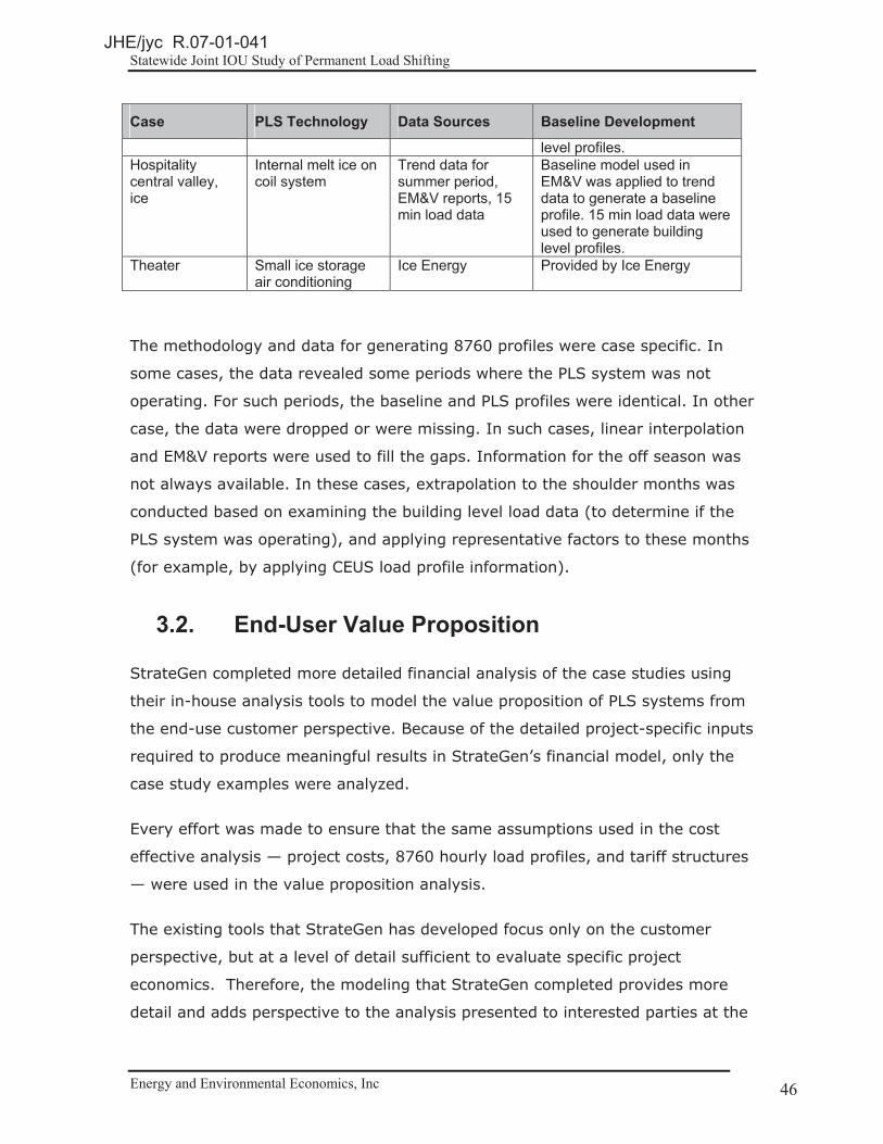
Statewide Joint IOU Study of Permanent Load Shifting
Energy and Environmental Economics, Inc Page 46 46
Case PLS Technology Data Sources Baseline Development
level profiles. Hospitality central valley, ice
Internal melt ice on coil system
Trend data for summer period, EM&V reports, 15 min load data
Baseline model used in EM&V was applied to trend data to generate a baseline profile. 15 min load data were used to generate building level profiles.
Theater Small ice storage air conditioning
Ice Energy Provided by Ice Energy
The methodology and data for generating 8760 profiles were case specific. In
some cases, the data revealed some periods where the PLS system was not
operating. For such periods, the baseline and PLS profiles were identical. In other
case, the data were dropped or were missing. In such cases, linear interpolation
and EM&V reports were used to fill the gaps. Information for the off season was
not always available. In these cases, extrapolation to the shoulder months was
conducted based on examining the building level load data (to determine if the
PLS system was operating), and applying representative factors to these months
(for example, by applying CEUS load profile information).
3.2. End-User Value Proposition
StrateGen completed more detailed financial analysis of the case studies using
their in-house analysis tools to model the value proposition of PLS systems from
the end-use customer perspective. Because of the detailed project-specific inputs
required to produce meaningful results in StrateGen’s financial model, only the
case study examples were analyzed.
Every effort was made to ensure that the same assumptions used in the cost
effective analysis — project costs, 8760 hourly load profiles, and tariff structures
— were used in the value proposition analysis.
The existing tools that StrateGen has developed focus only on the customer
perspective, but at a level of detail sufficient to evaluate specific project
economics. Therefore, the modeling that StrateGen completed provides more
detail and adds perspective to the analysis presented to interested parties at the
JHE/jyc R.07-01-041

Statewide Joint IOU Study of Permanent Load Shifting
Energy and Environmental Economics, Inc Page 47 47
end-user level. Project specific details include the PLS equipment’s CAPEX,
OPEX, performance specifications, 8760 hourly electric bill savings, incentive
levels, tax effects, and other financial considerations for the entire lifecycle of the
project.
StrateGen’s analysis tools can also generate optimal sizing and dispatch of
certain categories of PLS technologies, such as batteries. Optimal dispatch
includes load leveling to maximize end-customer bill savings. The optimization
model uses historical 8760 hourly load data to calculate the optimal set points
for the charge and discharge of a battery system every day. The two battery
technology case examples were utilized to demonstrate what load leveling
dispatchability implies for the end user value proposition.
A detailed flow chart of StrateGen’s modeling approach is shown below:
Figure 8: Flow Chart of StrateGen's Value Proposition Analysis
�
Once each case example was loaded into the model, StrateGen then solved for
the incentive levels that stakeholders indicated would be required to drive
JHE/jyc R.07-01-041

Statewide Joint IOU Study of Permanent Load Shifting
Energy and Environmental Economics, Inc Page 48 48
customer adoption. For this study financial hurdles of three and five year simple
paybacks were utilized based on stakeholder feedback during the course of the
study. In addition to the simple payback hurdles, StrateGen solved for the
required incentive levels to achieve a 15% internal rate of return.
The incentive structures modeled to achieve these financial hurdles include $/kW
peak capacity shifted upfront incentives as well as TOU rate differential
requirements.
3.3. Market Assessment
The Project Team assumed that market size is not the primary limiting factor in
the development of a viable California PLS market. Economic constraints, such as
current system costs and ratepayer neutral incentive levels, will limit market
growth. Therefore, the analysis focuses on evaluating these constraints,
gathering feedback from industry stakeholders on drivers and barriers to
adoption, and assessing trends in existing PLS programs across the U.S.
The U.S. market overview was compiled through utility program websites, the
Database of State Incentives for Renewable Energy (DSIRE), and interviews with
utility program managers. Stakeholder feedback was gathered during interviews
with California IOU program personnel, third party vendors, engineers, PLS
technology suppliers, and others relevant to PLS (Table 8).
JHE/jyc R.07-01-041

Statewide Joint IOU Study of Permanent Load Shifting
Energy and Environmental Economics, Inc Page 49 49
Table 8: Stakeholder interviews
Utilities Program Managers SCE Cypress Ltd.
SDG&E EPS
PG&E Honeywell Utility Solutions Florida Power & Light Trane Glendale Water & Power Southern California Public Power Authority (SCPPA) Engineers OEMs ASW Engineering AIC/East PennCogent Energy Cristopia Ice BallsDavis Energy Group CALMACEnovity Ice EnergyInvensys Group International BatteryKS Engineers Prudent PowerLBNL PVT SolarMoudood Aslam Transphase CompanyRetrofit Originality Inc. Xtreme PowerSchneider Electric UC Davis Energy & Supply Chain Management
JHE/jyc R.07-01-041

Statewide Joint IOU Study of Permanent Load Shifting
Energy and Environmental Economics, Inc Page 50 50
4. Modeling Results
4.1. Cost-effectiveness
4.1.1. Avoided Cost Benefit Matrix
Figure 9 presents the broad scenario avoided cost results in graphical form for
the 66 idealized shift scenarios in climate zone 12. The avoided costs are in
present value benefits for the lifetime of the system, which is assumed to be 15
years unless stated otherwise (a sensitivity for 30 years was also performed),
and are normalized to peak kW capacity reduction. The kW peak capacity
reduction is defined as the maximum hourly change in energy reduction relative
to the profile baseline. We examined other normalization factors such as
average on peak period demand reduction or total kWh shifted per day, but kW
peak capacity reduction is used as the default metric because of its broad
applicability across various shift profiles and also its usefulness for comparison to
other capacity resources such as a combustion turbine.
Figure 9: Broad Scenario Analysis – Avoided Cost Benefits
$0
$500
$1,000
$1,500
$2,000
$2,500
$3,000
7 8 9 10 11 12 13 14 15 16 17
Avoi
ded�
Cost
�Ben
efits
�$/k
W�P
eak�
Capa
city
�Re
duct
ion
Shift�Start�Hour
1�Hour
2�Hours
4�Hours
6�Hours
8�Hours
10�Hours
JHE/jyc R.07-01-041

Statewide Joint IOU Study of Permanent Load Shifting
Energy and Environmental Economics, Inc Page 51 51
The present value of avoided cost benefits represent the total benefits to the
region as a whole (TRC), the utility (PAC) and ratepayers (RIM). The range of
avoided costs is wide and peaks at ~ $2,600/kW (representative of a daily 10
hour discharge from 10 AM to 8 PM). Shifts of 6 hours or more can achieve
avoided cost benefits above $2,000/kW shifted for many scenarios.
From a TRC and PAC perspective, a PLS system that has a total cost less than
the avoided costs will still provide net benefits. IN the RIM test, the bill impacts
of participants are compared to the avoided costs.
The matrix shows the value for a system that provides an identical absolute shift
each day of the year. It represents an upper bound of avoided cost benefits
that is unlikely to be achieved in practice. Because all values are in terms of kW
peak capacity reduction, a constant discharge across hours and days of the year
will show the maximum possible value for a given summer peak shift. Any
reduction of shift below the maximum discharge in certain hours, days or months
would simply lead to lower shift benefit values without changing the
normalization factor (peak capacity reduction). Consider two identical PLS
devices except that one runs year round and one runs only in the summer. Both
could have the same peak capacity reduction based on an hour occurring in the
summer. Both would therefore be normalized using the same factor. However,
the device running year round would have some additional benefits derived from
the shift benefits occurring in winter.
4.1.2. Bill Savings and Rate Payer Neutral Incentive
Figure 10 shows the bill savings for the 66 shift profiles under the generic rate.17
One important factor in the bill savings is that the baseline profile (the CEUS
generic commercial shape) peaks at ~ 12 pm. Therefore, shifts that occur after
12 pm do not accrue benefits for demand charge reductions and have lower total
bill savings.
17 Generic rate characteristics: Summer on peak energy charge $0.20/kWh, off peak charge $0.10/kWh; winter on peak charge is $0.12/kWh, off peak charge is $0.10/kWh; peak period all year is 12-6 pm Mon-Fri, excluding holidays. On peak demand charge is $10/kW all year round.
JHE/jyc R.07-01-041

Statewide Joint IOU Study of Permanent Load Shifting
Energy and Environmental Economics, Inc Page 52 52
Figure 10: Broad Scenario Analysis – Bill Savings Benefits – Generic Rate
$0
$200
$400
$600
$800
$1,000
$1,200
$1,400
$1,600
$1,800
$2,000
7 8 9 10 11 12 13 14 15 16 17
Bill�
Savi
ngs�
Bene
fits�
$/kW
�Pea
k�Ca
paci
ty�R
educ
tion
Shift�Start�Hour
1�Hour
2�Hours
4�Hours
6�Hours
8�Hours
10�Hours
The rate payer neutral incentive is defined to be the maximum incentive such
that the RIM test ratio is set to 1. For each profile in the analysis, the maximum
incentive is equal to the avoided cost benefits (Figure 9) minus the bill savings
benefits (Figure 10).
Figure 11: Broad Scenario Analysis – Rate Payer Neutral Incentive
$0
$200
$400
$600
$800
$1,000
$1,200
$1,400
$1,600
7 8 9 10 11 12 13 14 15 16 17
Equi
vale
nt�R
ate�
Paye
r�Neu
tral
�Ince
ntiv
e�Le
vels
�($/k
W)
Shift�Start�Hour
1�Hour
2�Hours
4�Hours
6�Hours
8�Hours
10�Hours
Figure 11shows that for shifts that begin at 12 pm or earlier, incentives average
~ $450/kW and range from $75 - $800/kW. The higher incentives shown for
JHE/jyc R.07-01-041

Statewide Joint IOU Study of Permanent Load Shifting
Energy and Environmental Economics, Inc Page 53 53
systems that begin after 12 pm are irrelevant as they would represent incenting
a PLS owner with additional money to run the PLS system less effectively.
As shown by Figure 11 under the broad scenario analysis some incentive levels
are possible to keep non-participating ratepayers unaffected. However, incentive
levels are generally lower than the incentives currently offered in pilots and
those cited by stakeholders as necessary incentive levels for spurring
investment. That said, specific rate structures and various rate options for
potential PLS customer can lead to widely differing results.
4.1.3. Sensitivity Analyses �
4.1.3.1. Sensitivity to Bill Savings and Rate Payer ���������Neutral Incentive
This section explores the sensitivity of rate payer neutral incentive levels to retail
rates. We repeated the previous broad scenario analysis with five California IOU
rates that span customer class and rate type (i.e., TOU with and without demand
charge, non-coincident and peak-time only demand charges). The customer is
assumed to be on the respective rate before installing the PLS system. Table 9
shows the upper bounds of rate payer neutral incentives.
Table 9: Upper Bound on Ratepayer Neutral Incentive Level Using Broad Scenario Analysis*
Minimum, Median and Maximum of Incentive ($/Peak kW reduction) +
2 Hours 4 Hours 6 Hours 8 Hours 10 Hours Generic Rate $210 $280 $360 $590 $645
$300 $460 $540 $630 $766 $370 $570 $570 $660 $805
PG&E A6 ($80) ($190) ($680) ($730) ($830)($20) ($60) ($250) ($680) ($810)
$90 ($20) ($150) ($460) ($790)PG&E A10 TOU S
$200 $560 $780 $1,020 $1,550 $350 $810 $1,220 $1,380 $1,600 $580 $1,160 $1,390 $1,560 $1,610
PG&E E20 P $190 $260 $100 $140 $500 $270 $370 $370 $430 $630 $310 $400 $490 $620 $660
SDG&E $200 $450 $250 $390 $840
JHE/jyc R.07-01-041

Statewide Joint IOU Study of Permanent Load Shifting
Energy and Environmental Economics, Inc Page 54 54
Minimum, Median and Maximum of Incentive ($/Peak kW reduction) +
2 Hours 4 Hours 6 Hours 8 Hours 10 Hours ALTOU $350 $520 $700 $760 $960
$580 $1,220 $1,400 $1,400 $1,450 SCE TOU-8B $350 $660 $840 $1,080 $1,920
$410 $860 $1,340 $1,650 $1,980 $590 $1,290 $1,710 $1,980 $2,010
* Assumes maximum shift on a daily basis, minimum cost period charging, and best discharge period. Does not include potential value in regulation or other ancillary services. For the PG&E tariffs, avoided costs were taken from climate zone 12; for the SDG&E tariff, avoided costs were taken from climate zone 10; and for the SCE tariff, avoided costs were taken from climate zone 14. Customer is assumed to be on the respective rate before implementing PLS. + Baseline profile is a general all commercial CEUS.
4.1.3.2. Seasonal Sensitivity
The subsequent figures explore the sensitivity of the avoided costs to two broad
seasons, the summer (May to October) and winter (November to April).
Figure 12: Broad Scenario Analysis – Avoided Costs Seasonal Sensitivity – May to October
$0
$500
$1,000
$1,500
$2,000
$2,500
7 8 9 10 11 12 13 14 15 16 17
Avoi
ded�
Cost
�Ben
efits
�$/k
W�P
eak�
Capa
city
�Re
duct
ion
Shift�Start�Hour
1�Hour
2�Hours
4�Hours
6�Hours
8�Hours
10�Hours
JHE/jyc R.07-01-041
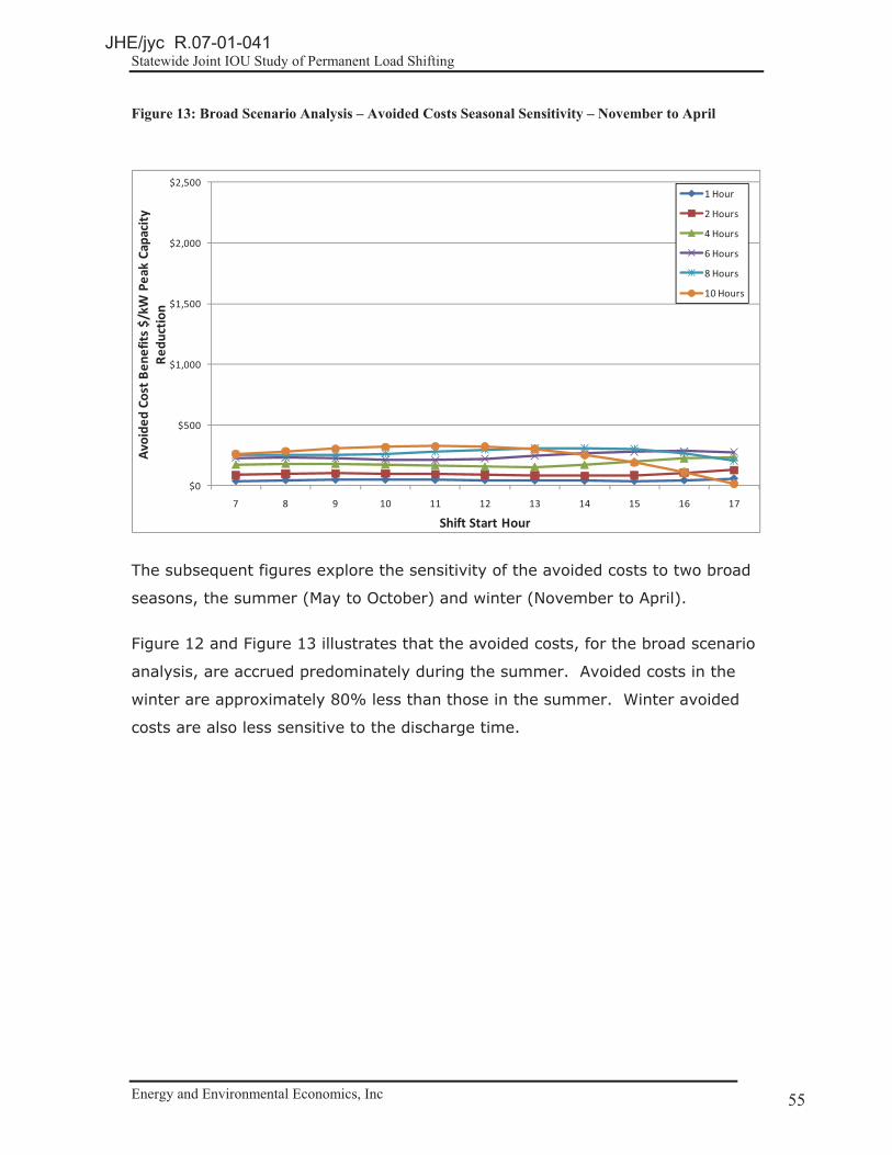
Statewide Joint IOU Study of Permanent Load Shifting
Energy and Environmental Economics, Inc Page 55 55
Figure 13: Broad Scenario Analysis – Avoided Costs Seasonal Sensitivity – November to April
$0
$500
$1,000
$1,500
$2,000
$2,500
7 8 9 10 11 12 13 14 15 16 17
Avoi
ded�
Cost
�Ben
efits
�$/k
W�P
eak�
Capa
city
�Re
duct
ion
Shift�Start�Hour
1�Hour
2�Hours
4�Hours
6�Hours
8�Hours
10�Hours
The subsequent figures explore the sensitivity of the avoided costs to two broad
seasons, the summer (May to October) and winter (November to April).
Figure 12 and Figure 13 illustrates that the avoided costs, for the broad scenario
analysis, are accrued predominately during the summer. Avoided costs in the
winter are approximately 80% less than those in the summer. Winter avoided
costs are also less sensitive to the discharge time.
JHE/jyc R.07-01-041

Statewide Joint IOU Study of Permanent Load Shifting
Energy and Environmental Economics, Inc Page 56 56
Figure 14: Broad Scenario Analysis – Bill Savings Seasonal Sensitivity – May to October
$0
$200
$400
$600
$800
$1,000
$1,200
$1,400
$1,600
$1,800
$2,000
7 8 9 10 11 12 13 14 15 16 17
Bill�
Savi
ngs�
Bene
fits�
$/kW
�Pea
k�Ca
paci
ty�
Redu
ctio
n
Shift�Start�Hour
1�Hour
2�Hours
4�Hours
6�Hours
8�Hours
10�Hours
Figure 15: Broad Scenario Analysis – Avoided Costs Seasonal Sensitivity – November to April
$0
$200
$400
$600
$800
$1,000
$1,200
$1,400
$1,600
$1,800
$2,000
7 8 9 10 11 12 13 14 15 16 17
Bill�
Savi
ngs�
Bene
fits�
$/kW
�Pea
k�Ca
paci
ty�
Redu
ctio
n
Shift�Start�Hour
1�Hour
2�Hours
4�Hours
6�Hours
8�Hours
10�Hours
Figure 14 and Figure 15 show that the difference in summer and winter bill
savings is not as great as the difference in avoided costs savings. Bill savings
are roughly 60% less in winter than in summer but are still significant. These
broad scenario comparisons are made based on the generic rate. The
comparisons suggest that winter PLS operation is likely to impact bill savings
more than avoided costs.
JHE/jyc R.07-01-041

Statewide Joint IOU Study of Permanent Load Shifting
Energy and Environmental Economics, Inc Page 57 57
4.1.3.3. Sensitivity to Energy Efficiency
All previously shown results are based on a round-trip efficiency of 100%. The
next set of sensitivities varies the assumptions of energy efficiency for the broad
scenario analysis and looks at the avoided cost and bill savings impacts.
Figure 16: Broad Scenario Analysis – Avoided Costs Sensitivity to Energy Efficiency – 80%
�$100
$0
$100
$200
$300
$400
$500
$600
$700
$800
Avoi
ded�
Cost
�Ben
efits
�PV�
$/kW
�Pea
k�Ca
pacit
y�Re
duct
ion
Wind�Overgen
RPS�Adder
T&D
Capacity�Residual
Emissions
A/S
Losses
Energy�
JHE/jyc R.07-01-041

Statewide Joint IOU Study of Permanent Load Shifting
Energy and Environmental Economics, Inc Page 58 58
Figure 17: Broad Scenario Analysis – Avoided Costs Sensitivity to Energy Efficiency – 100%
�$100
$0
$100
$200
$300
$400
$500
$600
$700
$800Av
oide
d�Co
st�B
enef
its�P
V�$/
kW�P
eak�
Capa
city�
Redu
ctio
n
Wind�Overgen
RPS�Adder
T&D
Capacity�Residual
Emissions
A/S
Losses
Energy�
Figure 18: Broad Scenario Analysis – Avoided Costs Sensitivity to Energy Efficiency – 120%
�$100
$0
$100
$200
$300
$400
$500
$600
$700
$800
$900
Avoi
ded�
Cost
�Ben
efits
�PV�
$/kW
�Pea
k�Ca
pacit
y�Re
duct
ion
Wind�Overgen
RPS�Adder
T&D
Capacity�Residual
Emissions
A/S
Losses
Energy�
Figure 16, Figure 17, and Figure 18 show the monthly avoided cost benefits
broken out by avoided cost components for a single shift profile among the 66
included in the broad scenario analysis. The shift profile examined here is a 10
JHE/jyc R.07-01-041
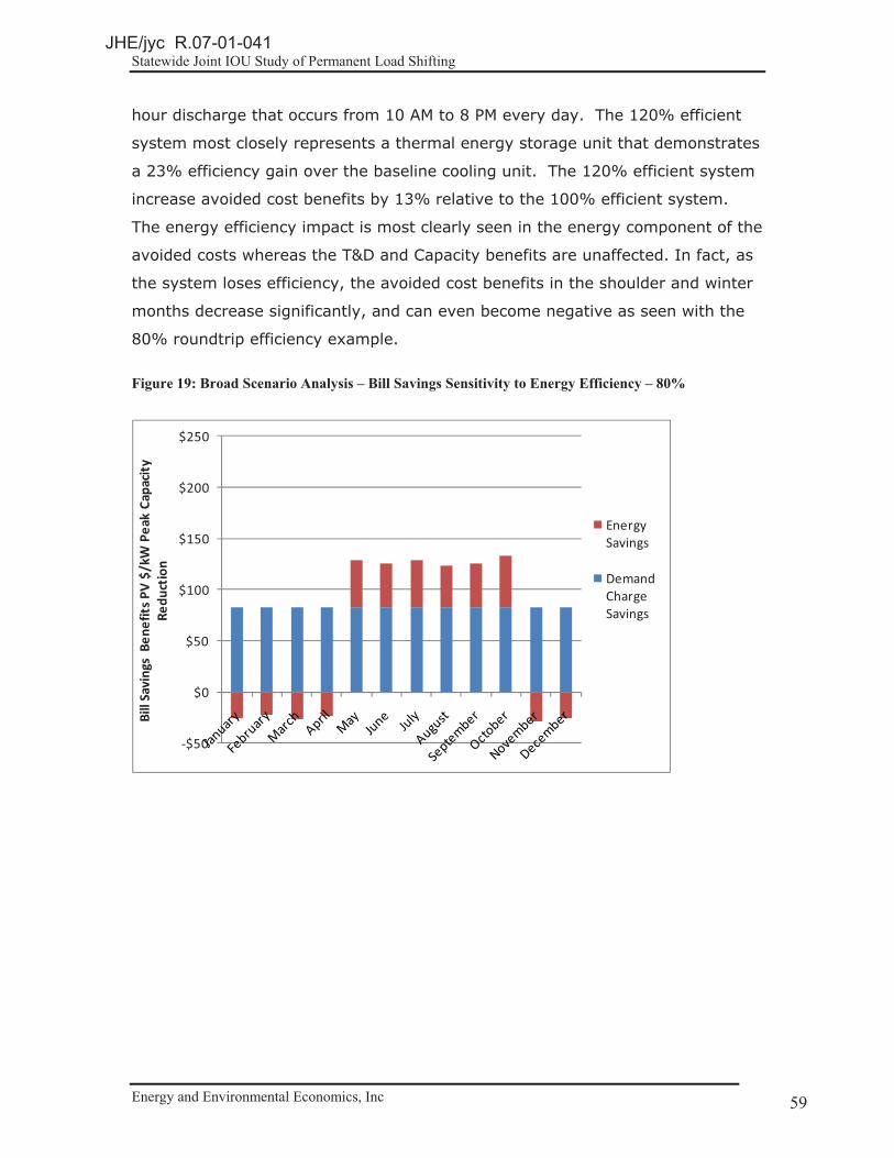
Statewide Joint IOU Study of Permanent Load Shifting
Energy and Environmental Economics, Inc Page 59 59
hour discharge that occurs from 10 AM to 8 PM every day. The 120% efficient
system most closely represents a thermal energy storage unit that demonstrates
a 23% efficiency gain over the baseline cooling unit. The 120% efficient system
increase avoided cost benefits by 13% relative to the 100% efficient system.
The energy efficiency impact is most clearly seen in the energy component of the
avoided costs whereas the T&D and Capacity benefits are unaffected. In fact, as
the system loses efficiency, the avoided cost benefits in the shoulder and winter
months decrease significantly, and can even become negative as seen with the
80% roundtrip efficiency example.
Figure 19: Broad Scenario Analysis – Bill Savings Sensitivity to Energy Efficiency – 80%
�$50
$0
$50
$100
$150
$200
$250
Bill�
Savi
ngs�
Bene
fits�P
V�$/
kW�P
eak�
Capa
city�
Redu
ctio
n
Energy�Savings
Demand�Charge�Savings
JHE/jyc R.07-01-041

Statewide Joint IOU Study of Permanent Load Shifting
Energy and Environmental Economics, Inc Page 60 60
Figure 20: Broad Scenario Analysis – Bill Savings Sensitivity to Energy Efficiency – 100%
�$50
$0
$50
$100
$150
$200
$250
Bill�
Savi
ngs�
Bene
fits�P
V�$/
kW�P
eak�
Capa
city�
Redu
ctio
n
Energy�Savings
Demand�Charge�Savings
Figure 21: Broad Scenario Analysis – Bill Savings Sensitivity to Energy Efficiency – 120%
�$50
$0
$50
$100
$150
$200
$250
Bill�
Savi
ngs�
Bene
fits�P
V�$/
kW�P
eak�
Capa
city�
Redu
ctio
n
Energy�Savings
Demand�Charge�Savings
Figure 19, Figure 20, and Figure 21 show the monthly bill savings benefits
broken out by bill savings components for the three energy efficiency scenarios,
using the generic tariff. Energy efficiency has more impact on bills than on
JHE/jyc R.07-01-041

Statewide Joint IOU Study of Permanent Load Shifting
Energy and Environmental Economics, Inc Page 61 61
avoided cost benefits. The 120% efficient system increases bill savings benefits
by 27% as compared to 16% for avoided costs. The 80% efficient system
reduces benefits by ~40% as opposed to ~30% for avoided costs.
4.1.3.1. Sensitivity to T&D Avoided Costs
Some stakeholders have suggested that PLS systems should not accrue avoided
cost benefits from deferring T&D investments. Figure 22 shows a 10 hour
idealized shift with and without T&D avoided costs. The total lifecycle avoided
costs are 22% lower without T&D avoided costs.
Figure 22: Broad Scenario Analysis – Sensitivity to T&D Avoided Costs – 2010
�$100
$0
$100
$200
$300
$400
$500
$600
$700
$800
Avoi
ded�
Cost
�Ben
efits
�PV�
$/kW
�Pea
k�Ca
pacit
y�Re
duct
ion
�$100
$0
$100
$200
$300
$400
$500
$600
$700
$800
Wind�Overgen
RPS�Adder
T&D
Capacity�Residual
Emissions
A/S
Losses
Energy�
4.1.3.2. Sensitivity to Resource Balance Year
A sensitivity to resource balance year was explored. Currently there is sufficient
energy capacity to meet demand in California. The resource balance year is the
year in which energy demand is projected to increase such that new capacity
additions will be required. These additions are most likely to come in the form of
a combustion turbine. However, as detailed in The Avoided Cost Appendix A, the
resource balance year affects the value of capacity provided by a PLS system
that is expected to operate for 15 years or more from today. The default
resource balance year in the current avoided costs is 2015. Figure 23 shows
that if the resource balance year is set to 2010, meaning a new CT is required
for capacity today, then there is approximately a 7% in the total present value
avoided cost savings.
JHE/jyc R.07-01-041
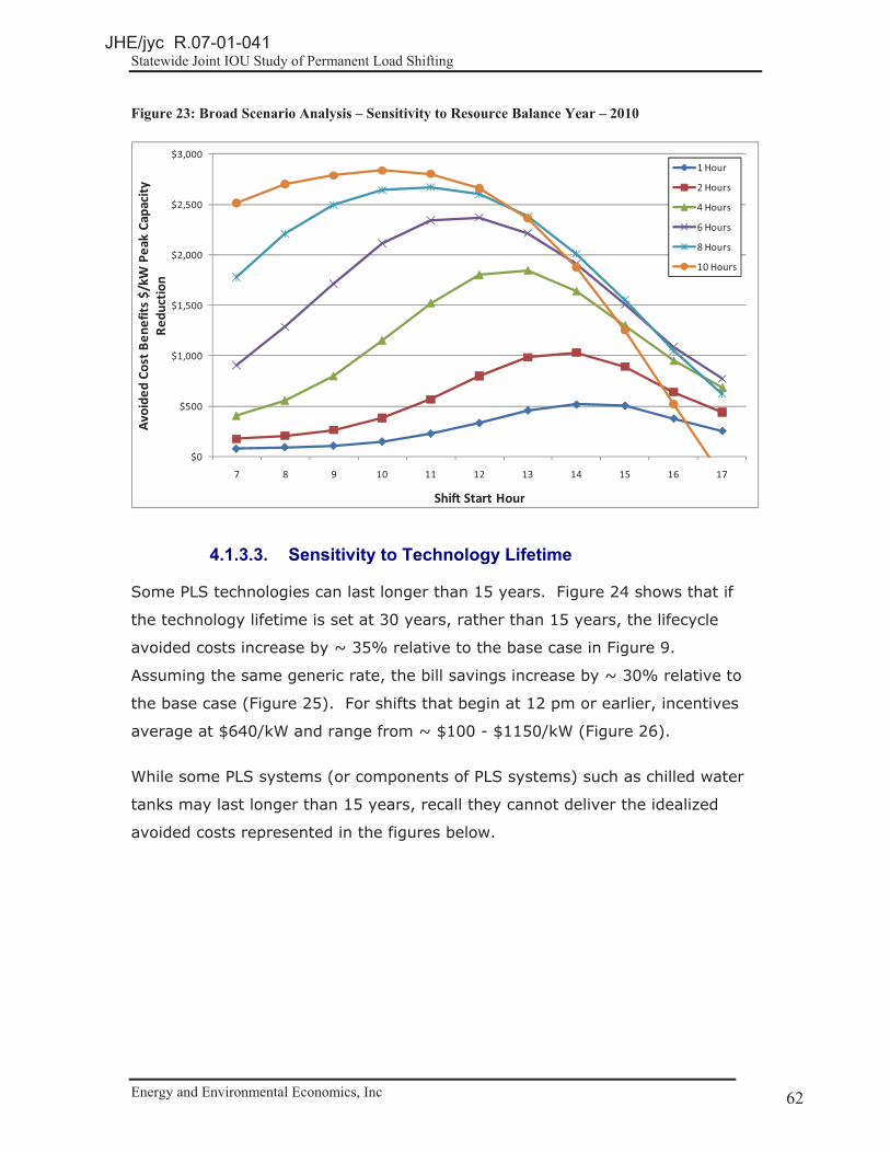
Statewide Joint IOU Study of Permanent Load Shifting
Energy and Environmental Economics, Inc Page 62 62
Figure 23: Broad Scenario Analysis – Sensitivity to Resource Balance Year – 2010
$0
$500
$1,000
$1,500
$2,000
$2,500
$3,000
7 8 9 10 11 12 13 14 15 16 17
Avoi
ded�
Cost
�Ben
efits
�$/k
W�P
eak�
Capa
city
�Re
duct
ion
Shift�Start�Hour
1�Hour
2�Hours
4�Hours
6�Hours
8�Hours
10�Hours
4.1.3.3. Sensitivity to Technology Lifetime
Some PLS technologies can last longer than 15 years. Figure 24 shows that if
the technology lifetime is set at 30 years, rather than 15 years, the lifecycle
avoided costs increase by ~ 35% relative to the base case in Figure 9.
Assuming the same generic rate, the bill savings increase by ~ 30% relative to
the base case (Figure 25). For shifts that begin at 12 pm or earlier, incentives
average at $640/kW and range from ~ $100 - $1150/kW (Figure 26).
While some PLS systems (or components of PLS systems) such as chilled water
tanks may last longer than 15 years, recall they cannot deliver the idealized
avoided costs represented in the figures below.
JHE/jyc R.07-01-041
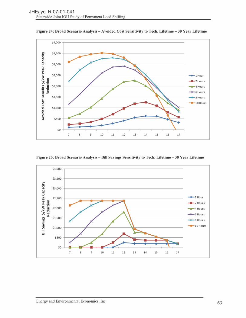
Statewide Joint IOU Study of Permanent Load Shifting
Energy and Environmental Economics, Inc Page 63 63
Figure 24: Broad Scenario Analysis – Avoided Cost Sensitivity to Tech. Lifetime – 30 Year Lifetime
$0
$500
$1,000
$1,500
$2,000
$2,500
$3,000
$3,500
$4,000
7 8 9 10 11 12 13 14 15 16 17
Avoi
ded�
Cost
�Ben
efits
�$/k
W�P
eak�
Capa
city
�Re
duct
ion
1�Hour
2�Hours
4�Hours
6�Hours
8�Hours
10�Hours
Figure 25: Broad Scenario Analysis – Bill Savings Sensitivity to Tech. Lifetime – 30 Year Lifetime
$0
$500
$1,000
$1,500
$2,000
$2,500
$3,000
$3,500
$4,000
7 8 9 10 11 12 13 14 15 16 17
Bill�
Savi
ngs�
$/kW
�Pea
k�Ca
paci
ty�
Redu
ctio
n
1�Hour
2�Hours
4�Hours
6�Hours
8�Hours
10�Hours
JHE/jyc R.07-01-041

Statewide Joint IOU Study of Permanent Load Shifting
Energy and Environmental Economics, Inc Page 64 64
Figure 26: Broad Scenario Analysis – Rate Payer Neutral Incentive Sensitivity for Assumed Technology Lifetime of 30 Years
$0
$500
$1,000
$1,500
$2,000
$2,500
7 8 9 10 11 12 13 14 15 16 17
1�Hour
2�Hours
4�Hours
6�Hours
8�Hours
10�Hours
4.1.3.4. Energy Basis Sensitivity
The results shown, thus so far, have been in units of $/kW Peak Capacity
Reduction. The value, on an energy basis, offers some insight. For example,
when using $/kW as a metric, the 10 hour duration batteries typically result in a
higher value because they shift more total energy throughout the day. For some
technologies, however, the cost of installed energy is a constraint. Therefore, it
is useful to see when energy is most valuable to discharge.
Figure 27 represents the same set of scenarios as presented in Figure 9 but with
the avoided costs normalized to the average daily kWh shifted. By using this
metric, the highest value duration and start hour profiles are not the 10 hour
durations, but rather the 1 and 2 hour durations. A 1- or 2-hour duration
starting a 2 pm provides the highest avoided cost benefit on an equivalent
energy basis. For battery technologies with limited installed energy and
customizable discharge power, a short duration output in the afternoon provides
the most grid value.
JHE/jyc R.07-01-041

Statewide Joint IOU Study of Permanent Load Shifting
Energy and Environmental Economics, Inc Page 65 65
Figure 27: Broad Scenario Analysis – Avoided Cost on an Energy Basis
$0.00
$0.02
$0.04
$0.06
$0.08
$0.10
$0.12
$0.14
$0.16
$0.18
7 8 9 10 11 12 13 14 15 16 17
Dai
ly�A
void
ed�C
ost�B
enef
its�$
/kW
h�D
eliv
ered
Shift�Start�Hour
1�Hour
2�Hours
4�Hours
6�Hours
8�Hours
10�Hours
4.1.3.5. Sensitivity to Additional Ancillary Services Revenues
Ancillary services are additional benefit values that some PLS technologies may
be able to accrue, though this capability has yet to be demonstrated. Regulation
and Spinning Reserve are modeled as values that a PLS technology could accrue
in addition to the permanent load shift product. As theoretical values we chose
to model these values as an upper bound for what a PLS technology might be
able to accrue in the ancillary services markets. For our modeling of regulation,
the PLS technology bids into the regulation up market whenever it is charging or
full and bids into the regulation down market whenever it is discharging or
empty. For spinning reserve, the technology bids into the spinning reserve
market whenever it is fully charged. In practice, there are factors such as an
energy-biased regulation signal and imperfect foresight which would reduce the
value of the ancillary services benefits shown in Figure 28 and Figure 29.
The ancillary service benefits used are 15 year projections of ancillary services
values which have the same hourly shape as the 2009-2010 CAISO historical
values corresponding to our avoided cost energy price period. These historical
JHE/jyc R.07-01-041

Statewide Joint IOU Study of Permanent Load Shifting
Energy and Environmental Economics, Inc Page 66 66
values were then escalated into the future at the same rate as our projected
escalation of energy prices in the avoided cost model.
Figure 28: Broad Scenario Analysis – Sensitivity to Ancillary Services – 6 Hour Duration
Energy
A/S
Capacity
T&D
Wind�Overgen
RegulationSpinning�Reserve$0
$500
$1,000
$1,500
$2,000
$2,500
$3,000
Pres
ent�V
alue
�$/k
W�cu
stom
er�p
eak�
redu
ctio
n
+23%
+5%
Figure 29: Broad Scenario Analysis – Sensitivity to Ancillary Services – 1 Hour Duration
EnergyA/S
Capacity
T&D
Wind�Overgen
Regulation
Spinning�Reserve
�$100
$0
$100
$200
$300
$400
$500
$600
$700
Pres
ent�V
alue
�$/k
W�cu
stom
er�p
eak�
redu
ctio
n
+130%
+41%
JHE/jyc R.07-01-041

Statewide Joint IOU Study of Permanent Load Shifting
Energy and Environmental Economics, Inc Page 67 67
Figure 28 shows the additional values that regulation or spinning reserve could
provide to a PLS system that is able to participate in those markets. Figure 28
represents a 6 hour shift every day starting at 12 PM. Figure 29 represents a 1
hour shift everyday starting at 2 PM. Regulation and spinning reserve represent
greater incremental values to the avoided costs of the permanent load shift
product for the shorter duration discharge.
4.1.3.6. Summary of Avoided Cost Sensitivities�
Table 10 shows the sensitivities we ran to look at the avoided cost values. All
the sensitivities shown were carried out on idealized shift profiles. Table 10
shows the directionally impact of the sensitivities on avoided costs, as well as the
relative magnitude of each sensitivity.
Table 10: Summary of Avoided Cost Sensitivities
Avoided Cost
Sensitivities
Directional Impact Relative Magnitude in Terms of Lifecycle Avoided Costs
T&D The elimination of T&D avoided costs reduces total avoided costs.
For a 10 hour idealized shift, removing T&D avoided costs reduces total avoided cost benefits by ~20%.
Seasonal Shift
A shift for only part of the year reduces avoided costs
Compared to a year-round shift, a shift from May to October reduces the broad scenario analysis avoided costs on average ~ 15%.
Energy Efficiency
A decrease in roundtrip efficiency reduces avoided costs
Compared to a 100% round-trip efficient system, an 80% round-trip efficient system reduces avoided costs by ~ 15% for a 10 hour idealized shift.
Technology Lifetime
A longer technology lifetime increases avoided costs.
A technology lifetime of 30 years increases the avoided costs by ~ 35%.compared to a 15 year lifetime.
Ancillary Services
Additional ancillary services capabilities increases avoided costs.
For a 6 hour idealized system, regulation benefits could supplement the avoided costs by ~25% and spinning reserve could increase value by ~5%.
Resource Balance Year
An earlier resource balance year increases avoided costs
A resource balance year of 2010 relative to the baseline resource balance year of 2015 increased avoided costs benefits by 7%.
JHE/jyc R.07-01-041

Statewide Joint IOU Study of Permanent Load Shifting
Energy and Environmental Economics, Inc Page 68 68
4.1.4. Specific Case Results: Simulated Scenarios
The cost effectiveness results for the simulated case studies are summarized in
Figure 30. The simulated thermal storage examples generally pass the TRC test,
while the simulated battery scenarios do not. The thermal storage examples
marginally fail the RIM test under the specific tariff (PG&E A10 TOU18), while
some battery examples pass the RIM test, depending on the load profile. The
battery examples were modeled using a TOU rate that included summer and
winter demand charges, as well as a noncoincident demand charge19.
Figure 31 summarizes the incentive levels for these same case studies based on
the RIM and PAC tests. Since the thermal storage examples do not pass the RIM
test, a negative rate payer neutral incentive level is estimated. This result
implies that the rate itself provides an incentive to the participant that is in
excess of the value of the PLS system. The PAC test incentive is roughly
$2000/kW (the avoided cost benefits) for these examples. The RIM test results
are mixed for the battery profiles. In some cases, the rate provides the incentive
— specifically for the load leveling examples. This result is not surprising, since
the battery operation was optimized for bill savings. The battery incentive, based
on the PAC test, is roughly $500-700/kW.
18 The PG&E A-10 TOU, as of November, 2010: on-peak to off-peak TOU energy differential of $.03/kWh in the summer and $.01/kWh in the winter. It also has peak day pricing rate of $.90/kWh which was modeled as being called on 15 days (the maximum allowable). In addition, there is an all-hours demand charge of $10.88/kW in summer and $6.53/kW in winter. 19 Characteristics of rate used to model battery scenarios: summer on peak energy charge of $0.11/kWh, off peak $0.07/kWh; winter on peak energy charge of $011/kWh, off peak $0.08/kWh; summer demand charge of $13/kW, winter demand charge of $5/kW; noncoincident demand charge of $13/kW.
JHE/jyc R.07-01-041

Statewide Joint IOU Study of Permanent Load Shifting
Energy and Environmental Economics, Inc Page 69 69
Figure 30: Summary of Simulated Example Cost Effectiveness
0.0
0.5
1.0
1.5
2.0
2.5
3.0
3.5
4.0
4.5
5.0
Sim�Office�CZ�3
Sim�Retail�CZ�3
Sim�Office�CZ�4
Sim�Retail�CZ�4
Sim�Office�CZ�12
Sim�Retail�CZ�12
Sim�Office�CZ�13
Sim�Retail�CZ�13
Manf�Facility,�
Lead�Acid�Battery,�Southern�
CA
Manf�Facility,�
Lead�Acid�Battery�
Load�Leveling,�Southern�
CA
Manf�Facility,�
Flow�Battery,�Southern�
CA
Manf�Facility,�
Flow�Battery�
Load�Leveling,�Southern�
CA
Thermal�Storage�Simulation Battery�Simulation
Bene
fit�to
�Cos
t�Rat
io
Cost�Effectiveness�Test�RatiosTRC�Test
RIM�Test
Figure 31: Summary of Simulated Examples Incentive Levels
�$1,000
$0
$1,000
$2,000
$3,000
$4,000
$5,000
$6,000
Sim�OfficeCZ�3
Sim�RetailCZ�3
Sim�OfficeCZ�4
Sim�RetailCZ�4
Sim�OfficeCZ�12
Sim�RetailCZ�12
Sim�OfficeCZ�13
Sim�RetailCZ�13
ManfFacility,
Lead�AcidBattery,
SouthernCA
ManfFacility,
Lead�AcidBattery
LoadLeveling,Southern
CA
ManfFacility,
FlowBattery,
SouthernCA
ManfFacility,
FlowBattery
LoadLeveling,Southern
CA
Thermal�Storage�Simulation Battery�Simulation
Upf
ront
�Ince
ntiv
e�in
�$/k
W�M
axim
um�P
eak�
Redu
ctio
n
Lifecycle�Benefit
3�year�Payback�Incentive
5�year�Payback�Incentive
Ratepayer�Neutral�Incentive�Levels
JHE/jyc R.07-01-041

Statewide Joint IOU Study of Permanent Load Shifting
Energy and Environmental Economics, Inc Page 70 70
Recall that eight partial shift chilled water scenarios were evaluated for two
building types (office & retail) for climate zones (3, 4, 12, and 13). The office
simulation in climate zone 3 is shown in Figure 32.
Figure 32: Specific Case Results – Simulation Office CZ 3
Energy
A/S
RPS�Adder TOU�EnergyCharge�Benefits
Capacity
T&D
DemandChargeBenefits
Wind�Overgen
IncrementalPLS�System
Costs$0
$500
$1,000
$1,500
$2,000
$2,500
$3,000
$3,500
Pres
ent�V
alue
�$/k
W�cu
stom
er�p
eak�r
educ
tion
Avoided�Costs
Bill�Savings
PLS�System�Costs
In this example, the PLS installation passes the TRC test, but fails the RIM test.
Based on a ratepayer neutral incentive cap, the system does not merit an
incentive. The RIM test result, however, is specific to the underlying tariff and
holds true only so long as the utility tariff stays consistent. The PLS system
costs are generally less than the bill savings, indicating a positive participant cost
test for the range of costs assumed20. This results imply that over the lifetime of
the project, the bill savings offset the cost of the PLS system.
The thermal storage examples are based on hourly outputs from an energy
simulation program. Because the eight sets of load shapes resulted in similar
cost-effectiveness results, individual figures for all cases are not shown.
20 As noted in Chapter 3, the system costs are estimated assuming $150-$400/ton-hr unit costs.
JHE/jyc R.07-01-041

Statewide Joint IOU Study of Permanent Load Shifting
Energy and Environmental Economics, Inc Page 71 71
4.1.5. Specific Case Results: PLS Pilots and Recent Installations
The Project Team performed a “retrospective” cost-effectiveness analysis of
recent installations. While it is not appropriate to make a policy decision on the
value of a program using cost effectiveness results of individual installations, real
data can provide some insight into how programs may be improved.
There are a number of caveats to interpreting the results presented:
� The results are based on historical performance, not “ideal” operation of
the PLS system.
� In some cases, PLS systems are designed with a certain load in mind. For
a variety of reasons, the historical data may not reflect that intended load
(such as due to weather or changes in operating conditions)
� All costs and benefits are normalized to the observed maximum peak
reduction, which may less than or greater than the design peak reduction,
a common metric used by manufacturers.
Figure 33 summarizes the cost-effectiveness test results from recent
installations. Most of the installations pass the RIM Test, which implies that the
current rate does not provide benefits to the participant at the rate at which the
PLS system provides grid level benefits. Some systems pass the TRC test, while
others do not.
The refrigerated warehouse shows the highest TRC test and highest RIM test,
which means that this type of system, based on the monitored period of
operation, provides greater societal level benefits than the cost of the system,
and at no cost to non-participating ratepayers. The relative low TRC test for
some of the other thermal systems does not mean that these systems cannot
provide benefits comparable to the cost of the system, but rather, they did not
over the monitored period.
JHE/jyc R.07-01-041

Statewide Joint IOU Study of Permanent Load Shifting
Energy and Environmental Economics, Inc Page 72 72
Figure 33: Summary of Case Results Cost Effectiveness
0.0
0.5
1.0
1.5
2.0
2.5
3.0
3.5
4.0
4.5
5.0
Office,�ChilledWater,�Southern
CA
Hospitality,�ChilledWater,�Central
Valley
Hospitality,�Med.Ice�System,�Central
Valley
RefrigeratedWarehouse,Southern�CA
Theater,�Small�IceSystem,�Southern
CA
Bene
fit�to
�Cos
t�Rat
io
Cost�Effectiveness�Test�RatiosTRC�Test
RIM�Test
Figure 34: Summary of Case Studies Incentive Levels
�$1,000
�$500
$0
$500
$1,000
$1,500
$2,000
$2,500
$3,000
$3,500
$4,000
$4,500
Office,�Chilled�Water,Southern�CA
Hospitality,�ChilledWater,�Central�Valley
Hospitality,�Med.�IceSystem,�Central
Valley
RefrigeratedWarehouse,�Southern
CA
Theater,�Small�IceSystem,�Southern�CA
Thermal�Storage�Installations
Upf
ront
�Ince
ntiv
e�in
�$/k
W�M
axim
um�P
eak�
Redu
ctio
n
Lifecycle�Benefit
3�year�Payback�Incentive
5�year�Payback�Incentive
Ratepayer�Neutral�Incentive�Levels
Actual�Incentive
Figure 34 provides estimates of the upfront incentive level that could be justified
based on the monitored data, using the PAC and the RIM tests. The actual
incentives provided by the IOUs, on a $/kW basis, are provided as well.
JHE/jyc R.07-01-041

Statewide Joint IOU Study of Permanent Load Shifting
Energy and Environmental Economics, Inc Page 73 73
For three of the scenarios (office, southern CA, refrigerated warehouse,
hospitality-chilled water), the equivalent ratepayer neutral incentive is positive,
with a maximum level of ~$1200/kW (the office building with chilled water). The
refrigerated warehouse example results in a ratepayer neutral incentive of ~
$800/kW. For both these examples, the actual incentive is less than the RIM and
PAC based incentives.
The hospitality examples both show PAC based incentives to be ~ $1000/kW and
ratepayer neutral incentives to be small. In these cases, the actual incentive is
roughly double the PAC incentive, although the incentive is applied to a
contracted kW reduction, not the “observed” peak reduction that is the
normalizing factor for the PAC and RIM test incentives.
The remainder of this section describes additional features of the examples.
Figure 35: Specific Case Results – Refrigerated Warehouse
Energy
A/SRPS�Adder
TOU�EnergyCharge�Benefits
Capacity
T&D
DemandChargeBenefits
IncrementalPLS�System
Costs
$0
$200
$400
$600
$800
$1,000
$1,200
$1,400
$1,600
Pres
ent�V
alue
�$/k
W�cu
stom
er�p
eak�r
educ
tion
Avoided�Costs
Bill�Savings
PLS�System�Costs
Figure 35 shows the cost effectiveness results of a refrigerated warehouse. The
tariff of the warehouse customer has a small ($0.03-$0.04/kWh) on-peak to off-
peak TOU energy differential. In addition, there are additive demand charges for
all-hours demand and on-peak demand. The demand charge for this example is
JHE/jyc R.07-01-041

Statewide Joint IOU Study of Permanent Load Shifting
Energy and Environmental Economics, Inc Page 74 74
based on 15 minute data. This system passes the TRC and RIM tests but does
not pass the participant test. The maximum ratepayer neutral incentive for this
system would be ~$1130/kW.
This system is a hybrid thermal – process shifting PLS technology. The
warehouse is precooled where the product within the warehouse serves as the
thermal storage entity. This PLS technology is infrastructure “light” in that the
load shifting was enabled through the installation of controls. Three key features
rendered this example to be an appropriate candidate for this technology.
� The unloading schedule of the warehouse was modified to facilitate
maintaining product temperature requirements during the peak period.
This process-shifting element was a key enabler and without it, the
warehouse would have been unable to load shift.
� The products held in this particular warehouse did not have FDA
regulations or other food regulations that prevented the use of this
technology.
� The climate is favorable to warehouse precooling.
This example was one of the most cost effective among the case studies;
however, this example has unique attributes and it’s not clear how many more
such opportunities exist.
JHE/jyc R.07-01-041

Statewide Joint IOU Study of Permanent Load Shifting
Energy and Environmental Economics, Inc Page 75 75
Figure 36: Specific Case Results – Office Chilled Water System – Historical Operation
Avoided�Costs
Bill�Savings
PLS�System�Costs
EnergyA/S TOU�Energy
Charge�Benefits
Capacity
T&D DemandCharge
Benefits
IncrementalPLS�System
Costs
$0
$500
$1,000
$1,500
$2,000
$2,500
$3,000
$3,500Pr
esen
t�Val
ue�$
/kW
�cus
tom
er�p
eak�
redu
ctio
n
Figure 36 shows historic data for an office chilled water system in Southern
California. This customer’s rate includes a TOU energy charge differential of
$0.07/kWh and $0.02/kWh in the summer and winter, respectively. The
demand charge is based on all hours demand. The office chilled water system
does not pass the TRC or participant tests but passes the RIM test. The
maximum ratepayer neutral incentive is estimated at ~ $690/kW.
JHE/jyc R.07-01-041

Statewide Joint IOU Study of Permanent Load Shifting
Energy and Environmental Economics, Inc Page 76 76
Figure 37: Specific Case Results – Office Chilled Water System –Improved Operation
Figure 37 shows an improved scenario for the same office chilled water system.
This scenario deviates from the historical operation in three distinct ways: the
energy efficiency upgrades that were in process during the monitored period are
assumed to be complete, the charging of the TES is assumed to begin at 11 pm
rather than 6 pm, and the TES operates all year round (the actual data showed
large periods where the TES did not operate). The lifecycle avoided costs are
~15% higher, relative to the historic profile (on an absolute basis) and bill
savings are nominally higher. The system passes the RIM test, with an estimated
maximum ratepayer neutral incentive of $840/kW. The example does not pass
the TRC or participant tests.
The office building example has some unique characteristics. While the facility
had a TES tank in place, it was not used for shifting, but as an additional chiller
when the existing chiller capacity could not maintain load; however, due to poor
engineering, the TES was not effective as a “third” chiller. The incremental PLS
system cost includes the engineering and controls improvements which provided
JHE/jyc R.07-01-041

Statewide Joint IOU Study of Permanent Load Shifting
Energy and Environmental Economics, Inc Page 77 77
energy efficiency improvements (~ 40%) and the cost to engineer and install a
TES tank of comparable size. The actual cost of this system (less the tank cost)
is less than the incremental cost shown above, but this comparison is not
appropriate for comparing with the estimated avoided costs. An additional
distinction is that the TES achieves a 30 °F temperature differential (“Delta T”)
rather than a typical 15 °F, which serves to reduce the all-in estimated cost.21
The modeled baseline reflects a conventional plant that met the full load with an
energy performance equivalent to the preretrofit cooling plant performance.
Figure 38: Specific Case Results – Hospitality, Chilled Water System, Central Valley
EnergyA/S
TOU�EnergyCharge�Benefits
Capacity
T&DDemandChargeBenefits
Wind�Overgen
IncrementalPLS�System
Costs
$0
$500
$1,000
$1,500
$2,000
$2,500
Pres
ent�V
alue
�$/k
W�cu
stom
er�p
eak�
redu
ctio
n
Avoided�Costs
Bill�Savings
PLS�System�Costs
Figure 38 shows data for a hospitality facility chilled water system in the Central
Valley. The tariff of this customer has an all-hours demand charge and a
summer on-peak demand charge, and a $0.06/kWh TOU energy charge
differential in summer and a $0.01/kWh TOU energy charge differential in winter.
21 The estimated cost is ~$2,700/kW for a 30 °F “Delta T” system (on a design-peak-reduction basis), but for a 15 °F Delta T, the cost would have been ~$4000/kW.
JHE/jyc R.07-01-041

Statewide Joint IOU Study of Permanent Load Shifting
Energy and Environmental Economics, Inc Page 78 78
The demand charges are calculated using 15 minute data. The chilled water
system does not pass the TRC or participant test but passes the RIM test. The
maximum ratepayer neutral incentive would be $560/kW.
Figure 39: Specific Case Results – Hospitality, Medium Ice System, Central Valley
Energy
A/SRPS�Adder TOU�Energy
Charge�Benefits
Capacity
T&D
DemandChargeBenefits
Wind�Overgen
IncrementalPLS�System
Costs
$0
$200
$400
$600
$800
$1,000
$1,200
$1,400
Pres
ent�V
alue
�$/k
W�cu
stom
er�p
eak�
redu
ctio
n
Avoided�Costs
Bill�Savings
PLS�System�Costs
Figure 39 shows data for a hospitality facility medium ice system in the Central
Valley. The tariff of this customer has an all-hours demand charge and a
summer on-peak demand charge, a $0.06/kWh TOU energy charge differential in
summer and a $0.01/kWh TOU energy charge differential in winter. The demand
charges for this example are calculated using 15 minute data. The chilled water
system does not pass the TRC or participant test but passes the RIM test. The
rate payer neutral incentive would be $380/kW.
In general, the thermal storage systems did not provide avoided cost benefits
that matched either the broad scenario modeling results or the simulated chilled
water examples. Sub-optimal charging, round-trip efficiencies (inefficiencies),
and variable shifts throughout the year reduce the avoided costs.
JHE/jyc R.07-01-041

Statewide Joint IOU Study of Permanent Load Shifting
Energy and Environmental Economics, Inc Page 79 79
Figure 40: Specific Case Results – Theater, Small Ice System, Southern California
Avoided�Costs
Bill�Savings
PLS�System�Costs
EnergyA/S
RPS�Adder
TOU�EnergyCharge�BenefitsCapacity
T&DIncrementalPLS�System
Costs
Wind�Overgen
$0
$500
$1,000
$1,500
$2,000
$2,500
$3,000Pr
esen
t�Val
ue�$
/kW
�cust
omer
�pea
k�red
ucti
on
Figure 40 shows data for a theater facility small ice storage air conditioning
system in Southern California. The tariff has $0.33/kWh and $0.04/kWh TOU
energy charge differentials in summer and winter, respectively. This tariff has no
demand charge. The small ice system does not pass any of the CE tests.
Two caveats are important to viewing these results. First, the rate that was
applied is not reflective of the actual rate, but was selected because it represents
a TOU rate without demand charge, and can thus be applied to evaluate savings
where building level load data are not available. The actual savings to the
customer may be greater or lower, depending on the real rate. Second, Ice
Energy’s current business model is utility ownership22. Because the participant
does not pay for the installation, viewing the results from the participant cost
22 Per communication with Ice Energy, Ice Energy’s business model has changed significantly since the start of the PLS pilot program. Today, Ice Energy provides specific offset capacity (MWs) and offset energy (MWHs) under contract to a utility expressed as a $/kW offset, for a contract term typically 20 to 25 years. Ice Bear energy storage units are installed at no cost to customers, and these assets are aggregated and managed via a real-time control network in accordance with the utility’s business objectives.
JHE/jyc R.07-01-041

Statewide Joint IOU Study of Permanent Load Shifting
Energy and Environmental Economics, Inc Page 80 80
test under the new business model may not be significant because it will always
be positive (assuming positive bill savings).
Figure 41: Specific Case Results – Batteries
�$500
$0
$500
$1,000
$1,500
$2,000
$2,500
$3,000
$3,500
$4,000
$4,500
Pres
ent�V
alue
�$/kW
�cust
omer
�peak
�redu
ctio
n
Wind�Overgen T&D Capacity
RPS�Adder Energy IncrementalPLS�SystemCosts
TOU�EnergyCharge�Benefits
DemandChargeBenefits
Avoided�Costs
Bill�Savings
PLS�System�Costs
Avoided�Costs
Bill�Savings
PLS�System�Costs
Avoided�Costs
Bill�Savings
PLS�System�Costs
Avoided�Costs
Bill�Savings
PLS�System�Costs
Lead�Acid
Lead�Acid�Load�Level
Flow�Battery
Flow�Battery�Load�Level
Figure 41 shows the cost-effectiveness test for four battery examples. None of
the battery systems pass the TRC or the participant cost test, although the non-
load level scenarios for both batteries passes the RIM test because the demand
charge savings are lower. For non-load leveling outputs, the ratepayer neutral
incentive is $660/kW for the lead acid battery and $850/kW for the flow battery.
The tariff of the customer for all the batteries is the same. The tariff has an all-
hours demand charge and an on-peak demand charge year-round. The tariff
also has a $0.04/kWh TOU energy charge differential in summer and a
$0.03/kWh TOU energy charge differential in winter. The demand charge for this
example is calculated using hourly kWh data.
4.1.6. Case Studies: Generation Capacity Value�Sensitivities
The Project Team performed sensitivity analysis to the generation capacity value
to explore the effect of misalignment between the load data and avoided costs.
JHE/jyc R.07-01-041

Statewide Joint IOU Study of Permanent Load Shifting
Energy and Environmental Economics, Inc Page 81 81
For each simulated and real example, the idealized capacity value was
estimated. The idealized value is based on aligning the maximum daily
reductions with the capacity avoided costs in a way that maximizes their value.
Table 11 shows the relative increase in capacity value that result from assuming
idealized alignment between the avoided costs and load data. Figure 42 shows
the idealized capacity value alongside the estimated capacity value.
Table 11: Capacity value sensitivity
Example Idealized Value Increase over Base Capacity Value (%)
Sim Retail CZ 3 60% Sim Office CZ 3 35% Sim Retail CZ 4 35% Sim Office CZ 4 50% Sim Retail CZ 12 45% Sim Office CZ 12 65% Sim Retail CZ 13 45% Sim Office CZ 13 65% Hospitality, Med. Ice System, Central Valley 25% Hospitality, Chilled Water, Central Valley 15% Office, Chilled Water, Southern CA 30% Refrigerated Warehouse, Southern CA 15% Theater, Small Ice System, Southern CA 5%
The simulated chilled water scenarios show the greatest sensitivity to realigning
the data. The real installations would see at most a 30% increase in generation
capacity value, with some examples showing good alignment (e.g., theater small
ice system). These margins do not alter the main observations from the analysis.
JHE/jyc R.07-01-041

Statewide Joint IOU Study of Permanent Load Shifting
Energy and Environmental Economics, Inc Page 82 82
Figure 42: Case study analysis of ideal capacity value
4.2. End User Impacts
The purpose of the end user analysis is to estimate incentive levels that will drive
customer adoption of PLS technologies. This analysis looks exclusively at the
simulated and example case studies because project-specific details are required
to produce meaningful project-level value proposition results.
For each of the simulations and examples in the end user analysis, the same
load data, tariff structure, and system specification and costs were utilized as in
the cost effectiveness analysis section described in the sections above.
4.2.1. Project Paybacks before Incentives
Nearly all of the simulations and examples had paybacks periods to the end user
that were greater than 5 years (stakeholder feedback indicated that 5 year
payback periods are the current hurdle to drive commercial customer adoption of
JHE/jyc R.07-01-041

Statewide Joint IOU Study of Permanent Load Shifting
Energy and Environmental Economics, Inc Page 83 83
PLS equipment). In fact, only the “low cost” simulated stratified chilled water
scenarios demonstrated paybacks of less than 5 years without incentives. The
following chart lists the specific payback periods before the introduction of
incentives:
Table 12: Simulation and Example Payback Periods Before Incentives
Simple Payback Period (Years) Simulation/Example High Cost Average
Cost23Low Cost
Sim Office CZ 3 6.8 5.2 3.3 Sim Retail CZ 3 8.6 6.4 4.2 Sim Office CZ 4 12.2 8.7 5.6 Sim Retail CZ 4 7.2 5.5 3.5 Sim Office CZ 12 9.7 7.1 4.6 Sim Retail CZ 12 10.6 7.6 4.9 Sim Office CZ 13 10.9 7.8 5.0 Sim Retail CZ 13 11.7 8.3 5.4 Sim PLS 4h PLS Mfg Flow Batt N/A24 Sim PLS 4h Mfg Lead Acid Batt N/A Sim Load Leveling 4h Mfg Flow Batt N/A Sim Load Leveling 4h Mfg Lead Acid Batt
9.5
Ex Office Building, Chilled Water, Southern California
N/A
Ex Hospitality, Chilled Water System, Central Valley
N/A
Ex Hospitality, Medium Ice System, Central Valley
9.5
Ex Refrigerated Warehouse, Southern California
8.5
23 Average cost data available for all examples, but only chilled water simulations include high and low cost estimates 24 N/A indicates that the project did not have a year in which cumulative cash flows become positive without incentives
JHE/jyc R.07-01-041

Statewide Joint IOU Study of Permanent Load Shifting
Energy and Environmental Economics, Inc Page 84 84
4.2.2. Incentive Level Requirements�
Based on the results of the section above before incentives are introduced for
PLS projects, these example projects would require some level of incentives to
drive customer adoption. Based on stakeholder feedback, payback periods of
three to five years are required to drive customer adoption. In order to calculate
what these incentive levels must be, StrateGen began the analysis with a simple
up front incentive payment in units of $/max kW shifted to off-peak. Then the
end user value proposition model solved for the $/max kW shifted incentive
levels required to achieve simple payback periods of three and five years. The
following graph overlays the simulations results of the required incentive levels
with the PAC and RIM Test rate-payer neutral incentive levels for comparison:
Figure 43: Simulation Required Incentive Levels vs. PAC & RIM Tests
�$1,000
$0
$1,000
$2,000
$3,000
$4,000
$5,000
$6,000
Sim�OfficeCZ�3
Sim�RetailCZ�3
Sim�OfficeCZ�4
Sim�RetailCZ�4
Sim�OfficeCZ�12
Sim�RetailCZ�12
Sim�OfficeCZ�13
Sim�RetailCZ�13
ManfFacility,
Lead�AcidBattery,
SouthernCA
ManfFacility,
Lead�AcidBattery
LoadLeveling,Southern
CA
ManfFacility,
FlowBattery,
SouthernCA
ManfFacility,
FlowBattery
LoadLeveling,Southern
CA
Thermal�Storage�Simulation Battery�Simulation
Upf
ront
�Ince
ntiv
e�in
�$/k
W�M
axim
um�P
eak�
Redu
ctio
n
Lifecycle�Benefit
3�year�Payback�Incentive
5�year�Payback�Incentive
Ratepayer�Neutral�Incentive�Levels
Figure 43 indicates that required incentive levels for the thermal storage
simulations range from about $100 to 1,000/kW to achieve a 5 year payback for
the end user and approximately $860 to $1,800/kW to achieve a 3 year
payback. The battery simulations’ required incentive levels range from $1,100 to
over $5,000 to achieve required payback levels. Several of the 3 and 5 year
payback incentive levels for the simulated examples are less than the PAC based
incentives but greater than the RIM based incentive levels.
JHE/jyc R.07-01-041

Statewide Joint IOU Study of Permanent Load Shifting
Energy and Environmental Economics, Inc Page 85 85
Figure 44 overlays the IOU pilot project results of the required incentive levels
with the PAC and RIM Test rate-payer neutral incentive levels for comparison:
Figure 44: IOU Pilot Project Required Incentive Levels vs. PAC & RIM Tests
�$1,000
�$500
$0
$500
$1,000
$1,500
$2,000
$2,500
$3,000
$3,500
$4,000
$4,500
Office,�Chilled�Water,Southern�CA
Hospitality,�ChilledWater,�Central�Valley
Hospitality,�Med.�IceSystem,�Central
Valley
RefrigeratedWarehouse,�Southern
CA
Theater,�Small�IceSystem,�Southern�CA
Thermal�Storage�Installations
Upf
ront
�Ince
ntiv
e�in
�$/k
W�M
axim
um�P
eak�
Redu
ctio
n
Lifecycle�Benefit
Ratepayer�Neutral�Incentive�Levels
Actual�Incentive
3�year�Payback�Incentive
5�year�Payback�Incentive
This graph of the IOU pilot projects above indicates that required incentive levels
for the thermal storage projects range from about $400 to 3,560/kW to achieve
a 5 year payback for the end user and approximately $700 to $1,800/kW to
achieve a 3 year payback. With the exception of the Refrigerated Warehouse
example, nearly all of the required incentive levels for the other examples are
greater than the RIM and PAC test levels. Also, as indicated by the black dot data
points, the office building and chilled water example actual pilot incentive levels
were less than the required incentive levels to achieve three or five year
paybacks. The medium ice and refrigerated warehouse actual pilot incentive
levels were much closer to the required incentive levels to achieve three or five
year paybacks.
JHE/jyc R.07-01-041

Statewide Joint IOU Study of Permanent Load Shifting
Energy and Environmental Economics, Inc Page 86 86
4.2.3. Sensitivities to Incentive Level Requirements�
In addition to running required $/kW upfront incentive levels for three and five
year paybacks, StrateGen conducted the following sensitivities:
� Required $/kW upfront incentive to achieve a 15% internal rate of return
(IRR)
� On to off peak-peak TOU rate differential required to achieve a five year
payback
Table 13 compares the different required incentive levels to achieve a 15% IRR
versus a three and five year payback period:
Table 13: Comparison of incentive levels for three and five year paybacks
Required Upfront Incentive Level ($/kW) Simulation/Example 15% IRR
Hurdle 5yr Payback
Hurdle 3yr Payback
Hurdle Office, Chilled Water, Southern CA 3680 3030 3850 Hospitality, Chilled Water, Central Valley 2980 2410 2810 Hospitality, Med. Ice System, Central Valley 760 660 1040 Refrigerated Warehouse, Southern CA 500 440 740 Theater, Small Ice System, Southern CA 2900 2400 3110 Sim Office CZ 3 -50 80 860 Sim Retail CZ 3 560 570 1410 Sim Office CZ 4 1470 1290 2120 Sim Retail CZ 4 80 160 840 Sim Office CZ 12 730 690 1400 Sim Retail CZ 12 1010 920 1690 Sim Office CZ 13 950 850 1540 Sim Retail CZ 13 1200 1070 1810 Manf Facility, Lead Acid Battery, Southern CA 2440 1980 2290 Manf Facility, Lead Acid Battery Load Leveling, Southern CA 1330 1150 1790 Manf Facility, Flow Battery, Southern CA 6000 4820 5350
For most of the simulations and example cases, the 15% IRR hurdle equates to
required incentive levels between the three to five year payback hurdles. The
JHE/jyc R.07-01-041
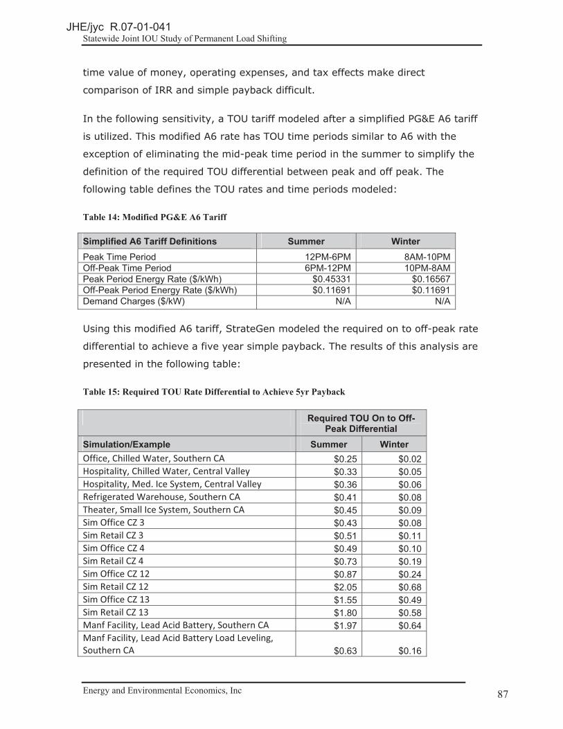
Statewide Joint IOU Study of Permanent Load Shifting
Energy and Environmental Economics, Inc Page 87 87
time value of money, operating expenses, and tax effects make direct
comparison of IRR and simple payback difficult.
In the following sensitivity, a TOU tariff modeled after a simplified PG&E A6 tariff
is utilized. This modified A6 rate has TOU time periods similar to A6 with the
exception of eliminating the mid-peak time period in the summer to simplify the
definition of the required TOU differential between peak and off peak. The
following table defines the TOU rates and time periods modeled:
Table 14: Modified PG&E A6 Tariff
Simplified A6 Tariff Definitions Summer Winter Peak Time Period 12PM-6PM 8AM-10PM Off-Peak Time Period 6PM-12PM 10PM-8AM Peak Period Energy Rate ($/kWh) $0.45331 $0.16567 Off-Peak Period Energy Rate ($/kWh) $0.11691 $0.11691 Demand Charges ($/kW) N/A N/A
Using this modified A6 tariff, StrateGen modeled the required on to off-peak rate
differential to achieve a five year simple payback. The results of this analysis are
presented in the following table:
Table 15: Required TOU Rate Differential to Achieve 5yr Payback
Required TOU On to Off-Peak Differential
Simulation/Example Summer Winter Office,�Chilled�Water,�Southern�CA� $0.25 $0.02 Hospitality,�Chilled�Water,�Central�Valley� $0.33 $0.05 Hospitality,�Med.�Ice�System,�Central�Valley� $0.36 $0.06 Refrigerated�Warehouse,�Southern�CA� $0.41 $0.08 Theater,�Small�Ice�System,�Southern�CA� $0.45 $0.09 Sim�Office�CZ�3� $0.43 $0.08 Sim�Retail�CZ�3� $0.51 $0.11 Sim�Office�CZ�4� $0.49 $0.10 Sim�Retail�CZ�4� $0.73 $0.19 Sim�Office�CZ�12� $0.87 $0.24 Sim�Retail�CZ�12� $2.05 $0.68 Sim�Office�CZ�13� $1.55 $0.49 Sim�Retail�CZ�13� $1.80 $0.58 Manf�Facility,�Lead�Acid�Battery,�Southern�CA� $1.97 $0.64 Manf�Facility,�Lead�Acid�Battery�Load�Leveling,�Southern�CA� $0.63 $0.16
JHE/jyc R.07-01-041

Statewide Joint IOU Study of Permanent Load Shifting
Energy and Environmental Economics, Inc Page 88 88
Manf�Facility,�Flow�Battery,�Southern�CA� $0.33 $0.05
From the required TOU differential table above, the spreads required to achieve
a five year payback vary significantly depending on the simulation or example
pilot project. The required spread varies from $0.25/kWh to over $2.00/kWh in
the summer months and from $0.02/kWh to $0.67/kWh in the winter months.
This is primarily due to PLS system efficiency and total project cost.
JHE/jyc R.07-01-041

Statewide Joint IOU Study of Permanent Load Shifting
Energy and Environmental Economics, Inc Page 89 89
5. Market Issues and Stakeholder Feedback
5.1. State of the Industry
This section first provides an overview of other programs around the country,
highlighting different program types, incentive levels and key takeaways. A
summary of stakeholder input gathered during interviews or feedback submitted
after workshop sessions follows.
5.1.1. Permanent Load Shifting Programs
The following list represents an overview of load shifting programs around the
country, followed by a discussion of takeaways. The majority of the programs
presented here are utility-sponsored thermal energy storage incentive programs.
Other program types include special TOU rate structures or technology-neutral
load shifting programs. This information was compiled through utility program
websites, the DSIRE website, and interviews with utility program managers and
other industry stakeholders.
5.1.1.1. Program Overview
Anaheim Public Utilities (California)25
Program: TES and TOU
Anaheim Public Utilities offers business and industrial customers a thermal
energy storage incentive of up to $21,000. The program objectives emphasize
financial savings, peak energy shifting, and energy savings. Eligible systems
include refrigerant-based thermal energy storage air conditioning systems and
ice storage units approved under Title 24; central plant, chilled water circulation
cooling systems are not eligible. Participating customers may also qualify for a
new time-of-use thermal energy storage rate. Eligible customers include those
25 Anaheim Public Utilities program details can be found here: http://www.anaheim.net/article.asp?id=4132
JHE/jyc R.07-01-041

Statewide Joint IOU Study of Permanent Load Shifting
Energy and Environmental Economics, Inc Page 90 90
shifting a minimum of 20% of the monthly maximum on-peak demand to off-
peak as a result of thermal energy storage installations. If the customer fails to
shift 20% of demand, or exceeds 500 kW for a given meter for any 3 months
over a 12 month period, they are deemed ineligible for this special
developmental rate.
This program is currently fully subscribed and will not accept new applications for
funding until July 1, 2011.
Austin Energy (Texas)26
Program: TES, TOU, and Feasibility Incentive
Austin Energy's Power Saver™ program offers incentives for thermal energy
storage projects. In order to make smaller installations more attractive, rebates
are tiered based on system size: $300/kW for 0-100 kW shift; $150/kW for 100-
500 kW shift; $50/kW for >500 kW shift or higher. Participating customers are
required to shift between 20% and 50% of on-peak summer demand or 2,500
kW (whichever is less). Austin Energy requires a feasibility study for projects
with anticipated demand shift of 100kW or greater, and offers a 50% feasibility
study incentive, up to $7000. Participants must be billed for electricity on any
demand rate and use the TES TOU rider.
According to a Summit Blue report commissioned by SCE, “since incentives are
very low, interest in this product is minimal.”27
26 Austin Energy program details can be found here: http://www.austinenergy.com/Energy%20Efficiency/Programs/Rebates/Commercial/Commercial%20Energy/thermalEnergyStorage.htm27 Summit Blue, 2009, pg. 24
JHE/jyc R.07-01-041

Statewide Joint IOU Study of Permanent Load Shifting
Energy and Environmental Economics, Inc Page 91 91
Burbank Water and Power (BWP) (California)28
Program: TES
BWP's Energy Solutions program provides businesses with thermal energy
storage rebates of $800/kW of peak demand saved. Incentives are capped at
25% of the installed cost of the measure, and range from $4728 to $8544,
depending on the size and age of the unit installed. Additionally, the annual
customer rebate total may not exceed $100,000.
Connecticut Light and Power (CL&P)29
Program: Peak Demand Reduction
CL&P's Demand Reduction program offers commercial and industrial customers
guidance regarding customer electricity usage, including strategies to reschedule
usage to off-peak. In the first stage, a CL&P representative will analyze the
facility's electricity usage patterns and develop a proposal for installing or
implementing measures based on these findings. Incentives are available to
offset the cost of recommended upgrades. Eligible projects include reset
temperature controls, lighting controls, water cooler controls, vending machine
controls, water heater controls, process controls, HVAC controls, and
miscellaneous load controls. However, all projects are approved on a case-by-
case basis, so additional measures that perform load rescheduling or curtailment
may be eligible for incentives. After the measures are completed and the
demand reduction and energy savings have been verified, the customer receives
the incentive payment.
28 BWP program details can be found here: http://www.burbankwaterandpower.com/index.php/incentives-for-businesses/energy-solutions-business-rebate-programs29 CL&P program details can be found here: http://www.cl-p.com/Business/SaveEnergy/LoadManagement/DemandReduction.aspx
JHE/jyc R.07-01-041

Statewide Joint IOU Study of Permanent Load Shifting
Energy and Environmental Economics, Inc Page 92 92
Duke Energy (Ohio30, North Carolina31, South Carolina32)
Program: TES
Duke Energy's Smart $aver® Incentive Program offers thermal energy storage
incentives in Ohio, North Carolina, and South Carolina. Businesses can receive
$190/kW shifted for thermal energy storage systems with less than a MW shift.
For larger systems, businesses can apply for custom incentives. Used equipment
is not eligible for incentives, nor is equipment that is already receiving an
incentive from a different Duke Energy program.
Florida Power and Light (FPL)33
Program: TES, TOU and Feasibility Incentive
FPL provides incentives for businesses, schools and colleges to install thermal
energy storage systems. Participating customers receive $2500 toward a pre-
approved feasibility study conducted by a professional engineer, as well as $464-
$580 per ton of cooling load removed from the summer on peak period. The
actual incentive level depends on the equipment installed. FPL provides an
additional $16 to $20 per ton for initial commissioning. A TOU rate is available to
all Florida IOUs, which improves system payback. FPL has incorporated a
seasonal demand rate which significantly shortens the peak period window (from
9 to 3 hours), which has allowed customers to design systems based on a much
smaller window, and thus reduce costs.
The program is technology neutral, but technologies typically installed include
static ice and chilled water systems. Marketing for the program involves a two-
fold approach: a direct sales model targeting large customers, and an indirect
30 Duke Energy Ohio program details can be found here: http://www.duke-energy.com/ohio-large-business/energy-efficiency/chillers-thermal-storage.asp31 Duke Energy North Carolina program details can be found here: http://www.duke-energy.com/north-carolina-large-business/energy-efficiency/nclb-smart-saver-incentives.asp32 Duke Energy South Carolina program details can be found here: http://www.duke-energy.com/south-carolina-large-business/energy-efficiency/sclb-smart-saver-incentives.asp33 FPL program details were gathered during an interview with FPL and from here: http://www.fpl.com/business/energy_saving/programs/interior/thermal.shtml
JHE/jyc R.07-01-041

Statewide Joint IOU Study of Permanent Load Shifting
Energy and Environmental Economics, Inc Page 93 93
sales modeling targeting the design community. According to FPL, working with
the design community has been a very effective approach, as it allows them to
indirectly market to a number of customers through one design firm. FPL also
offers workshops and seminars throughout the state to outline program
incentives and guidelines.
Gulf Power (Florida)34
Program: Residential TOU
Gulf Energy's Energy Select program offers residential customers a special
“Residential Service Variable Pricing” (RSVP) rate. The RSVP rate features four
different prices based on time of day, day of week, and season. Customers who
opt in are required to purchase an Energy Select thermostat in order to
reschedule central heating and cooling, electric water heating, and pool heating
to run more in the lower price periods and less in peak periods. The program
also includes opportunities to participate in demand response events via remote
communication with the Energy Select thermostat.
Longmont Power and Communications (LPC) (Colorado)35
Program: TES
As a part of Longmont's Commercial Energy Efficiency Program, businesses can
receive up to $500/kW for thermal energy storage systems (as well as a number
of other technologies that perform energy efficiency measures such as lighting,
heating, and controls). Only commercial rate customers by LPC and Platte River
Power Authority are eligible.
34 Gulf Power program details can be found here: http://www.gulfpower.com/energyselect/the_rate.asp35 LPC program details can be found here: http://www.ci.longmont.co.us/lpc/bus/eep_homepage.htm
JHE/jyc R.07-01-041

Statewide Joint IOU Study of Permanent Load Shifting
Energy and Environmental Economics, Inc Page 94 94
MidAmerican Energy (Iowa36, Illinois37, South Dakota38)
Program: TES
As a part of MidAmerican's Energy Advantage program, non-residential
customers can receive incentives to purchase and install high-efficiency building
systems equipment. The program focuses primarily on space heating and cooling
systems, and provides incentives for eligible thermal energy storage systems.
The specific rebate level is customized based on incremental cost, peak demand
reduction, annual energy use reduction and annual energy cost savings. Other
equipment types that qualify include (but are not limited to) boilers over 2.5
million Btu input capacity; ground-source heat pump systems 135 million Btu/hr
or greater; premium-efficiency motors over 200 HP; process boiler, chiller and
refrigeration improvements; energy management systems; direct-fired heating
systems; thermal energy storage; variable air volume conversions; waste-
recovery systems; process and heat-recovery heat pumps; new and replacement
window systems; and insulation upgrade projects.
As of March 2009, there were only two customers participating in the program.39
Minnesota Power40
Program: TOU
Minnesota Power offers a Controlled Access/Storage Heating rate for residential
and commercial space heating and water heating in off-peak periods. Eligible
storage includes storage room units, a central storage furnace, a central hot
water system, or slab heat. Off-peak is defined as 11pm to 7am. Residential off-
36 MidAmerican Energy Iowa program details can be found here: http://www.midamericanenergy.com/ee/ia_bus_custom_systems.aspx37 MidAmerican Energy Illinois program details can be found here: http://www.midamericanenergy.com/ee/il_bus_custom_systems.aspx38 MidAmerican Energy South Dakota program details can be found here: http://www.midamericanenergy.com/ee/sd_bus_custom_systems.aspx39 Summit Blue, 2009, pg. 22. 40 Minnesota Power program details can be found here: http://www.mnpower.com/customer_service/cost_savings/commercial_storage_offpeak_heating.htm
JHE/jyc R.07-01-041

Statewide Joint IOU Study of Permanent Load Shifting
Energy and Environmental Economics, Inc Page 95 95
peak rates are 3.943 cents per kWh, and require an $8 monthly service charge.
Commercial rates are divided into two rates: primary service is 3.643 cents per
kWh with a $10.50 monthly service charge; secondary service is 3.943 cents per
kWh and a $10.50 monthly service charge.
Minnesota Power also has a residential and commercial “Dual Fuel” program,
which incentivizes buildings with a non-electric back-up heating system to switch
away from electric heat during periods of high demand. However, this is an
event-based program, not a scheduled shift.
NYSERDA (New York)41
Program: TES
NYSERDA's Existing Facilities program provides performance-based incentives for
energy efficiency and peak demand reductions, including energy or thermal
storage systems. Eligible energy storage projects can receive rebates based on
geographic location: the “Upstate” rebate is $300/kW and the “Downstate”
rebate is $600/kW. The total incentive amount cannot exceed the lesser of
$2,000,000 or 50% of the project cost. In addition, performance-based projects
must qualify for an incentive of at least $10,000.
Otter Tail Power (Minnesota, North Dakota, South Dakota)42
Program: TES
Otter Tail Power provides rebates of $10 to $60 per kW for new thermal storage
systems. The incentive level varies based on the rate on which the system is
installed, and requires a minimum installation of 9 kW. The RDC rate provides
$20/kW and applies to systems up to 100 kW. The Deferred-load rate offers
$30/kW up to 200 kW, then $10/kW up to 1,000 additional kW. The Fixed-time-
41 NYSERDA program details can be found here: http://www.nyserda.org/programs/Existing_facilities/default.html42 Otter Tail Power program details can be found here: http://www.otpco.com/SaveEnergyMoney/Rebates.asp
JHE/jyc R.07-01-041

Statewide Joint IOU Study of Permanent Load Shifting
Energy and Environmental Economics, Inc Page 96 96
of-delivery rate provides rebates of $60/kW up to 200 kW, then $20/kW for up
to 1,000 additional kW. Qualified systems include thermal storage central
furnaces, room units, underfloor cable or panel systems, or electric boilers
installed to serve underfloor systems.
Progress Energy Florida (PEF)43
Program: TES
PEF provides business customers incentives for installing thermal energy storage
systems. Eligible customers can receive up to $300/kW of reduced cooling load
during peak hours, and also have the option of taking advantage of a time-of-
use rate to improve savings. PEF provides a free “business energy check” as an
initial step, which will determine eligibility and provide guidance. Only new
equipment is eligible, and customers must perform a preliminary feasibility study
in order to receive any incentives.
Southern California Public Power Authority (SCPPA)44
Program: Utility-Owned TES
In January 2010, SCPPA announced a 53 MW distributed energy storage
program, with a goal of “reducing exposure to costly peak power and improving
the reliability of the electrical grid.”45 SCPPA has partnered with Ice Energy in
order to offer a utility-owned, cafeteria-style program to member utilities. In
terms of compensation, SCPPA has contracted to pay Ice Energy a set per-
project payment, and has budgeted for an annual “health check” and minor
maintenance. The program has currently subscribed 8 MW, with Glendale Water
and Power as the first utility to get approved and move forward. Glendale is
currently installing approximately ten Ice Energy units a week, and anticipates
43 PEF's program details can be found here: http://www.progress-energy.com/custservice/flacig/efficiency/index.asp44 SCPPA program details were gathered during an interview with SCPPA and from here: http://www.scppa.org/pages/misc/press.html45 SCPPA Press Release: http://www.scppa.org/pages/misc/press.html
JHE/jyc R.07-01-041

Statewide Joint IOU Study of Permanent Load Shifting
Energy and Environmental Economics, Inc Page 97 97
installing over 250 units by the end of this year. Utilities can hire local
contractors or work with Ice Energy installers.
According to SCPPA, a utility-owned business model is advantageous due to the
aggregate cost savings achieved through mass installations. In order to manage
the challenge of customer O&M issues, SCPPA has contracted with Ice Energy to
provide a 24 hour call center to handle initial calls from customers experiencing
problems.
TVA46
Program Type: TOU
Effective April 2011, Tennessee Valley Authority (TVA) will implement new
wholesale rates that will more accurately reflect the cost of power based on time
of use. The stated objectives of the change are “to reduce peak power demand
and find alternatives to building more expensive power plants.”47 Distributors
within TVA territory currently define rates based on general TVA guidelines, but
retain the authority to determine individual rate structures based on customer
needs. Under the new system, distributors will have the choice of two options:
the “Seasonal Demand or Energy Rate” or the “Time-of-Use Rate.” The Seasonal
Demand and Energy rate structure applies seasonal demand charges, with the
highest demand charges in summer. The Time-of-Use rate structure varies
pricing based on the season and time of day, with the highest rates in summer
afternoons.
TVA has offered TOU pricing to some large commercial and industrial customers
for several years, and reports significant benefits. Peak demand has been
reduced by several hundred MWs, and some participants have enjoyed up to
30% reductions on their bill. Starting in the fall, distributors will be allowed to
offer new TOU rates to commercial and industrial customers with over a MW of
demand. Customers with demand of over 5 MW will have the option of the
46 TVA rate details can be found here: www.tva.gov/news/releases/julsep10/Rate_Change.pdf47 www.tva.gov/news/releases/julsep10/Rate_Change.pdf
JHE/jyc R.07-01-041

Statewide Joint IOU Study of Permanent Load Shifting
Energy and Environmental Economics, Inc Page 98 98
existing firm rate, the new Time-of-Use rate, or a new Seasonal Demand and
Energy rate. These rate changes are designed to be revenue neutral for TVA.
5.1.1.2. Program Takeaways
Feasibility Studies
Funding feasibility studies improves outcomes and customer commitment, and is
a core part of many programs' incentive structure. FPL, which provides up to
$2500 for a pre-approved study conducted by a professional engineer, considers
the feasibility study requirement a key piece in program success. Austin Energy
also requires a feasibility study for projects with anticipated demand shift of
greater than 100 kW, and will fund up to 50% of the cost up to $7000. Progress
Energy also requires a feasibility study.
A feasibility study could potentially provide additional value by ensuring ongoing
monitoring. One suggestion by an industry stakeholder, in order to improve
monitoring, is to integrate monitoring into the feasibility study. For example, the
program could require engineers to commit to a specific level of monitoring as a
part of the feasibility study.
Special Rates
A number of programs offer special TES/PLS rates that accompany incentives,
which not only improve payback but encourage efficient system operation. For
example, Anaheim Public Utilities recently instituted a new “developmental” TOU
TES rate. Customers who fail to shift a minimum percentage of peak demand or
kW (whichever is less), are ineligible for the special rate. The program is
currently subscribed. FPL created a special seasonal demand rate, which shrinks
the peak period window from nine to three hours. A shorter peak period window
has allowed customers to design less costly systems, increasing the
attractiveness of the program. Other programs with special rates include Gulf
Power, Minnesota Power, and TVA.
JHE/jyc R.07-01-041

Statewide Joint IOU Study of Permanent Load Shifting
Energy and Environmental Economics, Inc Page 99 99
Adequate Incentives
Programs that do not provide an adequate up front incentive will struggle to
attract customers. Incentive levels vary widely, from $10/kW to $800/kW, with a
number of additional incentives, such as commissioning incentives or free
training programs, adding to the overall value. Some programs have struggled to
fully subscribe due to low incentives, such as Austin Energy, who offers tiered
rebates from $50-$300/kW based on program size.48 The available rates also
impact the success of an incentive. For example, interest in MidAmerican
Energy's program is limited due to relatively low on-peak rates.49 One option for
improving overall program success is offering a variety of incentives that address
different barriers. For example, FPL provides an incentive of $464-$580 per ton
for the equipment, with an additional $16-$20 per ton for initial commissioning
(performance testing), and $2500 to fund a feasibility study.
Ownership Models
Utility-ownership reduces costs through increased purchase volume. Focused
customer targeting, marketing, and capture can be more efficient and cost
effective given a utility’s knowledge base of its own customers. Utility-ownership
also eliminates the capital investment hurdle and TOU rate change risks
compared with customer-owned business models. However, utility ownership can
increase administrative costs and impose burdens on the utility. In order to avoid
issues with ongoing operations and maintenance, SCPPA contracted with Ice
Energy to provide a 24 hour call center to manage initial customer calls.
5.1.2. Stakeholder Feedback
While the following categories are not comprehensive, they represent highlights
from the most commonly expressed perspectives and observations throughout
the interview process. Feedback related to specific technologies has been taken
into account, but may not be explicitly stated in the summary feedback below.
48 Summit Blue, 2009, pg 24 49 Summit Blue, 2009, pg 22
JHE/jyc R.07-01-041
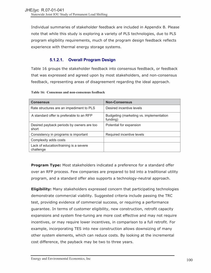
Statewide Joint IOU Study of Permanent Load Shifting
Energy and Environmental Economics, Inc Page 100 100
Individual summaries of stakeholder feedback are included in Appendix B. Please
note that while this study is exploring a variety of PLS technologies, due to PLS
program eligibility requirements, much of the program design feedback reflects
experience with thermal energy storage systems.
5.1.2.1. Overall Program Design
Table 16 groups the stakeholder feedback into consensus feedback, or feedback
that was expressed and agreed upon by most stakeholders, and non-consensus
feedback, representing areas of disagreement regarding the ideal approach.
Table 16: Consensus and non-consensus feedback
Consensus Non-Consensus Rate structures are an impediment to PLS Desired incentive levels
A standard offer is preferable to an RFP Budgeting (marketing vs. implementation funding)
Desired payback periods by owners are too short
Potential for expansion
Consistency in programs is important Required incentive levels Complexity adds costs Lack of education/training is a severe challenge
Program Type: Most stakeholders indicated a preference for a standard offer
over an RFP process. Few companies are prepared to bid into a traditional utility
program, and a standard offer also supports a technology-neutral approach.
Eligibility: Many stakeholders expressed concern that participating technologies
demonstrate commercial viability. Suggested criteria include passing the TRC
test, providing evidence of commercial success, or requiring a performance
guarantee. In terms of customer eligibility, new construction, retrofit capacity
expansions and system fine-tuning are more cost effective and may not require
incentives, or may require lower incentives, in comparison to a full retrofit. For
example, incorporating TES into new construction allows downsizing of many
other system elements, which can reduce costs. By looking at the incremental
cost difference, the payback may be two to three years.
JHE/jyc R.07-01-041

Statewide Joint IOU Study of Permanent Load Shifting
Energy and Environmental Economics, Inc Page 101 101
In terms of customer class, many respondents did not indicate a preference
based on a specific customer type (for example, commercial versus residential),
but instead based on cost and size. Larger systems are often more cost effective
than smaller systems. However, this observation led to differing conclusions,
with many stakeholders preferring a least-cost approach and thus large
commercial or industrial systems, and others indicating support for residential
systems because they were typically more expensive and thus more in need of
incentives.
Program Structure: Program structure preferences, such as the incentive level
or payment system, differed. One suggested option involved a single standard
offer paid directly to the end-customer (versus third party vendors). However,
technologies target different customer classes; a tiered standard offer may offer
more opportunities for additional technologies and customers to participate.
Program Consistency: Maintaining consistency in program requirements gives
rise to a number of benefits. For example, consistent, straightforward EM&V
requirements for each IOU could streamline the process, making participation
more attractive, increasing transparency, and potentially lowering costs.
Additionally, a consistent statewide standard offer would encourage commercial
customers, who may control multiple facilities, to participate throughout
California.
Program Complexity: As with consistency, while many requirements exist to
ensure outcomes, overly complex or burdensome requirements add to costs and
discourage participation. For example, rebate structures with complex
persistence payments can deter customers and increase the cost of program
administration.
Marketing: Challenges sourcing customers varied widely based on technology
and customer class. Demonstrating an attractive payback was the strongest
indicator of success, and there is also a category of customers who respond to
“green” marketing, and will opt in based on environmental attributes of a
system. In addition, targeting customers in the ideal rate class is challenging.
Marketing would be much more efficient if IOUS and third party vendors worked
JHE/jyc R.07-01-041

Statewide Joint IOU Study of Permanent Load Shifting
Energy and Environmental Economics, Inc Page 102 102
together to source customers: IOUs have access to confidential customer
information, including rate classes, and could initially screen and contact eligible
customers. Stakeholders also indicated that placing limitations on the type of
customer that can participate introduces significant barriers to program
subscription. Beyond utility-vendor collaboration, one option for improving
marketing efficiency is to work with the design community. Instead of targeting
individual customers, designers are often aware of multiple eligible projects,
which reduces marketing costs and also increases buy-in.
Training and Education: Lack of education and training for thermal energy
storage is a significant barrier, and needs to be taken into account when
estimating costs and potentially integrated into program design. Program
duration also limited training opportunities, and more established PLS programs
indicate a multiple year “learning curve,” leading to efficiency and lower costs in
the long term.
5.1.2.2. Incentives and Costs
Payback: Incentives need to align with acceptable payback periods for each
sector in order to drive demand. For the commercial sector, a two to three year
payback is generally necessary, although the economic downtown has placed
downward pressure on required payback periods. The public sector, along with
institutions such as college campuses, will accept longer payback periods of five
to seven years or more.
Comprehensive Approach: All market entry costs need to be taken into
account when determining incentive levels and cost effectiveness. Unexpected
costs, such as unanticipated structural engineering issues, architectural
requirements, or a limited number of contractors trained to do install, can all add
to overall program costs. In addition, each technology may require a different
skill set for installation, which should be considered in program design.
However, while private operating cost savings may not offset the cost of
implementing TES to the end-user, social benefits often do. In addition, building
power plants is extremely difficult and expensive, and may be subject to
additional regulations in the future which increase costs. Coal plant retirement
JHE/jyc R.07-01-041

Statewide Joint IOU Study of Permanent Load Shifting
Energy and Environmental Economics, Inc Page 103 103
will also place additional pressure on the system, and anticipating these needs
may be beneficial.
Rate Structure: The majority of respondents expressed interest in a more
favorable rate structure. Suggestions include creating a special PLS-specific
tariff, which could eliminate the need for any additional incentives in the form of
rebates or a standard offer. Eliminating off-peak demand charges will encourage
PLS, and on-peak demand charges could be increased to meet revenue neutrality
requirements.
“Tariff risk” is a significant concern, and many customers are unwilling to install
systems due to fear that the rate structure will change. Moreover, systems are
subject to the classic split incentive issue: the building engineer does not pay the
utility bills and thus is not motivated to reduce costs. Beyond guaranteeing more
favorable rates, allowing a shorter PLS peak period is another option for lowering
initial costs. In Florida Power and Light's TES program, customers requested a
shorter window for shifting, and were able to decrease system size and thus
overall cost. In addition, current rate schedules are too complicated, creating
additional challenges in system operation such as control sequences. However,
the tariff structure may need to be utility-specific.
Feasibility Studies: Many PLS programs provide funding for an initial feasibility
study, which can improve outcomes and customer commitment. See Program
Takeaways (Section 5.1.1.2) for additional background on the role of feasibility
studies in PLS programs.
Utility Financial Incentives: Utilities have a fiduciary responsibility to their
shareholders to provide a return on their investment, and installing PLS
technologies can be counter to this responsibility. If the utilities were able to
include properly designed and deployed PLS systems in their asset base, there
would be a large demand by utilities to deploy these technologies.
5.1.2.3. Performance
Baseline Data: For TES systems, it can be challenging to acquire baseline data
because the practice of monitoring, even of existing EMCS systems, is not typical
JHE/jyc R.07-01-041

Statewide Joint IOU Study of Permanent Load Shifting
Energy and Environmental Economics, Inc Page 104 104
practice. Sometimes, the expense of monitoring (if no instrumentation exists)
can be a challenge. This makes it difficult to measure the relative performance of
PLS systems. Establishing baseline for some processes – such as batch processes
– will be more challenging for industrial facilities than in buildings. For other PLS
technologies, such as batteries, monitoring is less challenging.
Additional Value Streams: Most PLS systems are not taking advantage of
additional value streams such as energy efficiency or demand response.
However, combining PLS and energy efficiency may lead to better overall system
design. For example, TES systems can range from energy neutral at the site to
site energy efficiency improvements of over 45%. At the same time, round trip
energy efficiency neutrality requirements may lead to additional complexity and
costs.
Operations and Maintenance: For the most part, ongoing operation and
maintenance costs were not a concern to respondents, although requirements
vary depending on customer class. For example, a residential or small
commercial system needs to be designed to limit ongoing maintenance.
Ongoing Performance and Monitoring: Energy efficiency and performance
monitoring is very important for existing facilities when upgrading an existing
TES or upgrading a non-TES to a TES system. Without monitoring, it is
impossible to identify poor operating strategies, and substantial energy waste
occurs. Specific measurement and verification requirements will differ based on
technology, such as installing a thermal meter on TES systems (for example, a
flow meter and temperature sensors entering and leaving the storage tank). A
monitoring requirement could be a part of the feasibility study. For example, the
program could require engineers to commit to a specific level of monitoring as a
part of the feasibility study. Alternatively, additional incentives could be provided
for monitoring, similar to FPL's current program, or incentives could be paid only
after a customer has demonstrated shift through system metering.
Existing Systems: A number of PLS systems were installed during previous
programs, or outside of any incentive structure. Many of these existing systems
are not run optimally, and there may be potential to “fine-tune” for less money
JHE/jyc R.07-01-041

Statewide Joint IOU Study of Permanent Load Shifting
Energy and Environmental Economics, Inc Page 105 105
than a full retrofit or a new install. For example, improving the temperature
differential for chilled water is essential for optimal operations, but many of
these systems are running at a very low differential.
JHE/jyc R.07-01-041

Statewide Joint IOU Study of Permanent Load Shifting
Energy and Environmental Economics, Inc Page 106 106
6. Program Design Recommendations
6.1. Overall Cost-effectiveness of PLS
6.1.1. Total Resource Cost Test
The Total Resource Cost test (Section 3.1.2.1) is typically used to evaluate
whether or not the CPUC should pursue a particular program. The test is used in
the evaluation of energy efficiency, distributed generation, demand response
programs and we use the same approach to evaluate PLS. The TRC compares
the avoided cost benefits to the region with the incremental50 cost of installing
and operating the PLS system, and the PLS program marketing and overhead
costs.
TRC = Avoided Cost Benefits –(Incremental PLS System Cost + PLS Program Admin Costs)
TRC perspective shows that the installed incremental cost of PLS technologies
must be in the range of $950/kW, $2,190/kW, and $2,640/kW to be cost-
effective for 2-hour, 6-hour, and 10-hour systems respectively ($475/kWh,
$365/kWh, $264/kWh).
Table 17: Upper Bound on Avoided Cost Benefits by Dispatch Type
Shift Duration Maximum Lifecycle Avoided Costs ($/peak kW reduction)
Maximum Average Daily Avoided Costs ($/kWh delivered/ day)
2 Hours $950 $0.17
4 Hours $1,700 $0.15
6 Hours $2,190 $0.13
8 Hours $2,480 $0.11
50 The term “incremental” refers to the “additional” cost of the PLS system. For example, in new construction, the PLS system may add some cost but achieve some cost savings in other places. The incremental cost incorporates the cost of the PLS system, minus the cost savings achieved elsewhere. For a retrofit application, the incremental cost is typically the entire cost of the PLS system.
JHE/jyc R.07-01-041

Statewide Joint IOU Study of Permanent Load Shifting
Energy and Environmental Economics, Inc Page 107 107
Shift Duration Maximum Lifecycle Avoided Costs ($/peak kW reduction)
Maximum Average Daily Avoided Costs ($/kWh delivered/ day)
10 Hours $2,640 $0.09
Assumptions: Assumes load reduction occurs during the highest value hours,
charging during the lowest cost hours (mainly 2am to 5am), and maximum shift
on all days of the year.
The results from the simulated and actual utility pilot data show lifecycle benefits
somewhat less than the best case shown in the table above. This is due to less
than ideal shifts on some days. However, the data from the actual systems we
evaluated is not a good predictor of maximum possible value since the systems
were operating to optimize local utility retail rates and not maximizing total
avoided costs. For example, a system might charge beginning at 8pm based on
the utility tariff, but this would be a higher cost time from an avoided cost
perspective than charging beginning at midnight or 2am.
Incremental system costs vary widely across different PLS technologies.
Thermal systems in the utility pilot programs are in the range ~ $1,000/kW to
$3,300/kW (normalized to the peak “observed” reduction, not design peak
reduction). Industry provided estimates that range from below $500/kW to as
high as $4,000/kW (where the costs are normalized to estimated peak
reductions). The dramatic range is due to differences between the costs for new
construction or expansion applications vs. retrofit applications, above ground vs.
below ground installations, and size of the application. For example, large chilled
water installations (such as those greater than 50,000 ton-hours) for new
construction and expansion applications that are above ground were cited to be
significantly less expensive than chilled water retrofit applications with the tanks
installed underground. Total installed battery storage costs are estimated to be
in the range of $1,800/kW to $4,030/kW for a discharge duration of 4-6 hours
($300-$1,010/kWh installed). Process shifting costs are expected to be broad,
ranging from very low to high.
JHE/jyc R.07-01-041

Statewide Joint IOU Study of Permanent Load Shifting
Energy and Environmental Economics, Inc Page 108 108
Table 18: Range of TRC Costs and Benefits by Technology Type Based on Case Studies
Technology Type Lifecycle TRC Benefit ($/kW)
Lifecycle TRC Cost* ($/kW)
Net Lifecycle TRC Benefits ($/kW)
‘Medium’ to ‘large’ thermal storage
$1,360-$2,670 $1,140-$3,310 ($1,950)- $1,020
Process shifting applications: Based on refrigerated warehouse
$1,315-$1,610 $750-$915 $570-$695
‘Small’ thermal storage systems: Based on Ice Energy Example
$1,380-$1,685 $2,460-$3,000 ($1,320)-($1,080)
Battery storage systems
$620-$880 $1,800-$4,030 ($3,400)-($924)
* Lifecycle cost does not include admin or other program costs; Costs for the examples are based on the capital costs normalized to the observed peak reduction, rather than a design peak reduction. + These categories included one example each; the range shown is based on assuming an uncertainty of ± 10% around the point estimate.
Comparison of the lifecycle benefits and the lifecycle costs indicates that well-
designed ‘medium’ and ‘large’ thermal systems pass the TRC test given current
costs and performance. While the range of costs for process shifting is large,
there are also undoubtedly applications that also pass the TRC. Potential
process shifting applications include timing the charging of electric batteries in
pallet jacks and forklifts, or shifting usage on electrical end uses such as
operation of pool pumps, or pumping load, or also specific industry processes
that can be designed to operate off-peak. Some applications such as pre-cooling
in refrigerated warehouses also pass the TRC test.
However, there are a number of emerging PLS technologies that do not pass the
TRC cost test given their current costs. The investor-owned utilities and CPUC
will have to decide whether to encourage these technology types. These include
most if not all of the technologies in the battery storage space providing PLS, as
well as ‘small’ thermal storage systems even assuming an idealized operating
profile.
Given this difference, it makes sense to divide the PLS market into mature and
emerging categories and have different program designs that are appropriate for
each.
JHE/jyc R.07-01-041
Statewide Joint IOU Study of Permanent Load Shifting
Energy and Environmental Economics, Inc Page 109 109
6.1.2. Considerations for a Market Transforming PLS Program
Whether to encourage the technologies that do not pass the TRC test today
depends on a wide range of factors. In particular, three key considerations of
whether PLS is a useful element in managing loads in the future should be
considered in rough order of importance.
Renewable Integration. PLS provides a high value use of electricity in low
load periods, reducing expected ‘overgeneration’ in the night time, particular in
Southern California as the state adds wind resources to meet the 33% RES
standard. Reducing overgeneration adds x% to the total value of PLS in the
modeling. Some PLS technologies also provide a ‘dynamic’ response that may
be able to provide regulations services or other system integration benefits.
Renewable integration will become an increasing concern as California adds
significant intermittent renewable generation capacity to meet the 33% RES.
Energy Efficiency. Some PLS designs have the potential to save not just cost,
but energy overall at the system level. Reducing energy use in California will
remain a priority in the long term. From this perspective, energy efficiency
should be considered from a ‘system’ perspective including reduction of higher
on-peak losses and generally worse efficiency of gas fired generation on peak.
Capacity Needs. PLS provides capacity by shifting loads from the peak period
to the off-peak thereby avoiding the need to build new generation capacity.
However, current reserve margins in California are extremely high (>30%) and
are forecasted to be above the planning reserve margin (PRM) beyond 2020.
There may be local capacity constraints, particularly if once-through-cooling
generation is retired, but capacity should not be a driving need for investing in
new technology development. As described in Section 3.1.4.1), however, some
parties argue that capacity incentives to demand-side resources should not
necessarily be limited to the short-run generation capacity value. They argue
that the priority placed on EE and DR in the loading order, and the need for
consistency in program offerings to attract and retain customers should support
higher incentives even in times of excess capacity.
JHE/jyc R.07-01-041
Statewide Joint IOU Study of Permanent Load Shifting
Energy and Environmental Economics, Inc Page 110 110
Given this outlook, the technologies that provide opportunity for renewable
integration, particularly dispatchable technologies, and overall system energy
efficiency seem particularly attractive technologies for California to encourage.
Technologies in this category include most electric storage (battery) technologies
as well as ‘small’ thermal storage systems.
To encourage these technologies, a ‘market transformation’ program could be
developed, geared toward creating manufacturing scale in the industry, as well
as local capability for PLS implementation; including design, construction, and
maintenance which will lead to lower costs and higher performance over time.
Today, California currently has a number of programs with market
transformation goals for other technologies including the California Solar
Initiative (CSI), and the Self-generation Incentive Program (SGIP).
6.1.3. Conclusions Based on the TRC Test
Create a ‘mature’ PLS program with the goal of maximizing the adopted MW of
cost-effective PLS technologies. The program should be available for all PLS
(‘technology neutral’) but will most likely encourage ‘medium’ and ‘large’ thermal
shifting technology (particularly for expansion and new construction
applications), as well as low cost process shifting and precooling. The emphasis
of the ‘mature’ PLS program category would be on achieving a high penetration
of economical, high performance systems.
Create a separate track for ‘emerging’ PLS technologies that provide renewable
integration and/or energy efficiency benefits with promise of long term cost
reductions with an emphasis on market transformation. Only select technologies
would be eligible for the higher ‘emerging’ PLS category including ‘small’ thermal
shifting devices (<10kW peak load shift) with dispatchable capability, and
electrical battery storage. The emphasis of the ‘emerging’ PLS program category
would be to develop a greater number of ‘load responsive’ technologies.
JHE/jyc R.07-01-041

Statewide Joint IOU Study of Permanent Load Shifting
Energy and Environmental Economics, Inc Page 111 111
6.2. PLS Program Design Framework – Standard Offer
There are a number of dimensions by which the CPUC can consider standard
offers for PLS program design. Perhaps the most fundamental dimensions have
to do with the basics of program structure and $ value of the incentive itself.
The following chart illustrates these dimensions, each with its own respective
continuum. For example, a PLS program at one end of the spectrum can have
no impact to ratepayers. In this case, the incentive would be essentially
‘ratepayer neutral’. At the other end of the spectrum would be incentives whose
level are set to ensure commercial adoption at the technology specific level,
perhaps based on achieving certain payback or internal rate of return
requirements by targeted end users. In this case, the incentive would be
focused on ‘market transformation’ similar to the California Solar Initiative (CSI)
or the California Self Generation Incentive Program (SGIP).
The other axis represents the PLS program structure – it can be geared toward
incentivizing energy shifting on peak, or, at the other end of the spectrum, be
more focused on pure capacity. The former, if paid on a “$/kWh of actual energy
shifted on-peak” would be purely performance based. The latter, if paid on a
$/kW capacity basis would require additional minimum requirements for
duration. The capacity-based incentive, for example, could be translated into a
$/kWh shifting capacity. Additional monitoring/verification would likely be
necessary with capacity based incentives to ensure performance compliance.
The CPUC’s goals with respect to PLS and any potential program will influence
where the program falls on these continuums, as well as the form of the
incentive itself. The chart below includes several examples of different
incentives that could be created – they are presented along the continuum of
energy/performance based vs. capacity based only, as the overall $ value of the
incentive can vary tremendously depending on the CPUC’s priorities with respect
to market transformation. Each will be described further below.
JHE/jyc R.07-01-041

Statewide Joint IOU Study of Permanent Load Shifting
Energy and Environmental Economics, Inc Page 112 112
Figure 45: Standard Offer Program Design Framework
PLS Tariff. PLS tariff could establish a fixed differential between peak and off
peak on an energy or $/kWh shifted on peak basis. Similarly, a PLS tariff that
shifted more cost from energy to on peak demand charges would provide a
financial incentive to shift demand from peak to off peak. A number of
stakeholders voiced strong support for establishing simple transparent tariffs
that would maintain their differentials between peak and off peak over many
years would be quite effective in stimulating development of PLS. A ‘PLS’ tariff
with TOU rate differentials provides some incentive to operate the PLS system
well, and does not require a specific baseline development. This approach is
more suitable for thermal storage. Specific PLS tariffs were also noted as a key
success criteria in many of the programs researched out of state, provided the
tariff was persistent for a number of years to help ensure project economic
viability.
Standard Offer. An alternative to creating a PLS specific tariff would be to pay
for kWh shifted on peak. A standard offer model based on an energy payment
($/kWh shifted) provides a direct performance-based incentive, but would
require strict guidelines for calculating baselines for thermal or process shifting
JHE/jyc R.07-01-041

Statewide Joint IOU Study of Permanent Load Shifting
Energy and Environmental Economics, Inc Page 113 113
PLS technologies. Therefore, this approach is easier to provide to electrical
battery systems. Shifted kWh could be metered/measured on site, and remotely
tracked. As stated earlier, measuring the kWh shift for thermal systems and
process shifting is more challenging than for battery systems, given their
baseline measurement requirements. It would be critical that such payments
would be of sufficient duration to provide economic certainty for any PLS project.
A comparable example to this form of incentive would be the current California
Solar Initiative, which pays an incentive pre-kWh generated.
Hybrid Standard offer. A combination of $/kWh shifted on peak as well as a
$/kW capacity based incentive could be used. PLS has a value for energy as well
as capacity – creating a hybrid incentive program could incentivize and reward
both.
Capacity Based Standard offer. Such a program could provide incentives
based on capacity shifted from peak to off peak. If a pure capacity incentive
were to be used, further clarification would need to be provided as to the
duration of the capacity shifting required to be eligible. As mentioned above,
capacity can be stated both in terms of kW and well as kWh. The kWh method
would automatically factor in the duration of shifting capability of the specific
technology. For capacity based standard offers, the performance that would
need to be verified would be the system’s ‘availability’. Because the incentive is
paid up front and not directly tied to performance (e.g., Actual kWh shifted on
peak), additional methods of ensuring accountability and performance would
need to be developed. The PG&E pilot, for example, requires detailed reporting
of energy shift and savings through its EM&V requirements.
One key advantage of standard offer program options is that they would
encourage technology development and innovation … provided they are
technology neutral. Further, a transparent standard offer would also enable a
diverse group of stakeholders to participate. An RFP approach, in contrast,
would likely need to specify the technology solution in advance, and qualified
bidders would be limited primarily to large firms capable of managing utility-
scale programs.
JHE/jyc R.07-01-041

Statewide Joint IOU Study of Permanent Load Shifting
Energy and Environmental Economics, Inc Page 114 114
Regardless of the form of the standard offer, simplicity, accountability and
persistence are key. Simplicity in that the program should be easily
communicated, implemented and monitored. Accountability in that the
incentives provided should be as closely tied to actual value delivered as
possible. Persistence in that the fundamental drivers of project economics need
to be in place for many years – sufficient for participants to realize economic
return from their investment.
The market transformation goals of the PLS program would similarly benefit from
adhering to these three core tenets. Simplicity, accountability and persistence
will facilitate the entry of new investors and other financial stakeholders, and
thus fuel the evolution of alternative ownership models to PLS deployment,
namely, third party owned systems and the availability of third party debt
financing for PLS projects. The availability of capital, both equity and debt are
critical to expanded implementation of PLS.
6.3. PLS Program Design Characteristics
Whether mature or emerging technology, the review of best practices
nationwide, and other data collected from technology providers leads to some
common recommendations for PLS program design, regardless of the PLS
technology or the ultimate incentive structure chosen.
Three stages of project execution are important to overall PLS success, including
system design, build and commission, and operations. Poor execution at any
stage can result in less than ideal benefits. The following diagram provides a
template program design that focuses on each stage.
JHE/jyc R.07-01-041

Statewide Joint IOU Study of Permanent Load Shifting
Energy and Environmental Economics, Inc Page 115 115
Figure 46: Recommended Characteristics of a PLS Program
While the details of design, performance testing51, and operations will be specific
to the type of technology and technology class, and more detailed for thermal
storage systems for example, all elements are applicable — and important — for
any type of PLS technology.
51 Functional performance testing is an important component of what is known as the commissioning process in the HVAC industry. The commissioning process is a process that ensures the building performs as per the owner’s intent. The functional performance testing component of commissioning is sometimes simply referred to as commissioning, such as in the Chapter 5 review of PLS markets where commissioning incentives are included.
JHE/jyc R.07-01-041

Statewide Joint IOU Study of Permanent Load Shifting
Energy and Environmental Economics, Inc Page 116 116
6.3.1. System Design
Provide Clear Incentive / Rate Signal for System Design
One of the key lessons learned from reviewing the PLS Pilot data and conversing
with stakeholders is that the PLS control algorithms are established to maximize
bill savings. Therefore, the PLS rate designs and / or other incentives associated
with performance must be clearly articulated and available during the system
design phase. There may be limited flexibility for some PLS technologies to
adjust the operations schedule significantly after the system is designed (such as
for process shifting and thermal systems). As discussed under incentives, there
are several choices to indicate preferred periods of performance including the
time schedule on time-of-use energy charges, time schedule on demand
charges, or a performance payment based on time of day.
The Joint Utilities should also consider defining ‘super off-peak’ periods to
indicate the relative value of charging during the middle of the night, rather than
at the beginning of the off-peak period. For example, in one real-world example
charging began at 8pm, which was the start of the off-peak period, although a
lower cost societal PLS system would charge beginning at midnight or 2am.
Require Technical and Economic Feasibility Study
The other ‘best practices’ lesson based on interviews around the country is that it
is important to require a technical feasibility study to ensure that the application
is engineered appropriately, and also establish a baseline against which to
measure performance during initial commissioning and ongoing operations. The
requirements of a technical feasibility study could vary by technology. The
process shifting and thermal storage PLS applications, by their nature, are
integrated into the overall operations of the host site and therefore warrant more
extensive technical feasibility approaches than electrical battery storage.
Smaller, ‘standard package’ systems might also have different technical
feasibility requirements. The requirements of the technical feasibility study that
should be considered include;
� System design and specifications
JHE/jyc R.07-01-041

Statewide Joint IOU Study of Permanent Load Shifting
Energy and Environmental Economics, Inc Page 117 117
� Forecasted baseline and modified cooling / process load shape as well as
expected whole building baseline and modified consumption profiles.
o Characterization of expected load modification: peak kW reduction,
expected shifted energy, system efficiency
o Minimum expected performance for use in EM&V studies(% shifted,
# days shifted, minimum efficiency)
� Financial/economic feasibility based on anticipated application, pre and
post load shape and applicable tariff
� Commissioning plan after project construction
� Monitoring plan for routine operations
6.3.2. Build and Test Performance
Require functional performance testing of the installation to verify that the PLS
system provides the load reduction identified in the technical feasibility study.
Good construction / installation and performance testing of the PLS systems is
also important to ensure the PLS system is working well. Therefore, the PLS
technologies should conduct a commissioning study and be required to provide a
commissioning report. Requirements of commissioning report may include;
o Verification that the system is installed and operating correctly and
as planned in the feasibility study and engineering drawings
o Verification that expected operation profile can be achieved
o Verification that the load modification metrics can be achieved
o Verification that the anticipated economic returns can be achieved
JHE/jyc R.07-01-041

Statewide Joint IOU Study of Permanent Load Shifting
Energy and Environmental Economics, Inc Page 118 118
6.3.3. Operations
Require regular reporting of operational data to verify persistence of good
performance.
A well designed system, if not operated well, will not provide anticipated system
benefits. Some of the PLS Pilot projects did not perform well in the field. The
need for an incentive to maintain excellent operations over time is the primary
driver behind the overall recommendation to provide to the extent possible a
performance based incentive based on kWh of energy actually shifted on peak.
Operational reports should be required to see if the PLS systems are performing
well, as expected in the project viability and commissioning studies, and are still
in service. Particularly with very flexible technologies such as electrical battery
storage, there may be significant opportunities to collect a PLS incentive and
operate in an alternative mode (such as an Uninterruptable Power Supply - UPS)
Along with the operational report, there should be some approach developed for
removing a customer from the PLS program when the facility is abandoned, is
not meeting performance levels or is no longer operational.
6.4. Establishing Incentive Levels for Standard Offer
To illustrate the range of possibilities with respect to the $ value of any incentive
(x axis of our framework, above), our study used two approaches. The first
approach is to calculate the ‘ratepayer neutral’ incentive level that could be
provided without a cross-subsidy from non-participating ratepayers. The second
approach is to calculate the incentive level required to attract reasonable
participation in the program. The balance of these two factors; ratepayer
subsidy on the one hand, and participation on the other, will be an important
part of overall program design, and highly dependent on CPUC goals/objectives
for PLS.
JHE/jyc R.07-01-041

Statewide Joint IOU Study of Permanent Load Shifting
Energy and Environmental Economics, Inc Page 119 119
6.4.1. Ratepayer Neutral Incentive Levels
The ratepayer neutral incentive level is predominantly driven by an expectation
of avoided cost benefits on the one hand, and the portion of those benefits that
are provided to the customer through the retail rate design on the other. If the
retail rate does not pass on all of the system benefits to the PLS customer, an
additional incentive can be provided without a subsidy.
As shown in the cost-effectiveness sections, the range of incentive level depends
on the amount of shift, and timing. The following table shows the range of
ratepayer neutral incentive levels.
Table 19: Upper Bound on Ratepayer Neutral Incentive Level Using Broad Scenario Analysis*
Minimum Median and Maximum of Incentive ($/Peak kW reduction) +
2 Hours 4 Hours 6 Hours 8 Hours 10 Hours Generic Rate $210 $280 $360 $590 $645
$300 $460 $540 $630 $766 $370 $570 $570 $660 $805
PG&E A6 ($80) ($190) ($680) ($730) ($830)($20) ($60) ($250) ($680) ($810)
$90 ($20) ($150) ($460) ($790)PG&E A10 TOU S
$200 $560 $780 $1,020 $1,550 $350 $810 $1,220 $1,380 $1,600 $580 $1,160 $1,390 $1,560 $1,610
PG&E E20 P $190 $260 $100 $140 $500 $270 $370 $370 $430 $630 $310 $400 $490 $620 $660
SDG&E ALTOU
$200 $450 $250 $390 $840 $350 $520 $700 $760 $960 $580 $1,220 $1,400 $1,400 $1,450
SCE TOU-8B $350 $660 $840 $1,080 $1,920 $410 $860 $1,340 $1,650 $1,980 $590 $1,290 $1,710 $1,980 $2,010
* Assumes maximum shift on a daily basis, minimum cost period charging, and best discharge period. Does not include potential value in regulation or other ancillary services. For the PG&E tariffs, avoided costs were taken from climate zone 12; for the SDG&E tariff, avoided costs were taken from climate zone 10; and for the SCE tariff, avoided costs were taken from climate zone 14. Customer is assumed to be on the respective rate before implementing PLS. + Baseline profile is a general all commercial CEUS.
JHE/jyc R.07-01-041
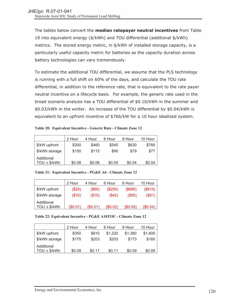
Statewide Joint IOU Study of Permanent Load Shifting
Energy and Environmental Economics, Inc Page 120 120
The tables below convert the median ratepayer neutral incentives from Table
19 into equivalent energy ($/kWh) and TOU differential (additional $/kWh)
metrics. The stored energy metric, in $/kWh of installed storage capacity, is a
particularly useful capacity metric for batteries as the capacity duration across
battery technologies can vary tremendously.
To estimate the additional TOU differential, we assume that the PLS technology
is running with a full shift on 60% of the days, and calculate the TOU rate
differential, in addition to the reference rate, that is equivalent to the rate payer
neutral incentive on a lifecycle basis. For example, the generic rate used in the
broad scenario analysis has a TOU differential of $0.10/kWh in the summer and
$0.03/kWh in the winter. An increase of the TOU differential by $0.04/kWh is
equivalent to an upfront incentive of $766/kW for a 10 hour idealized system.
Table 20: Equivalent Incentive - Generic Rate - Climate Zone 12
2 Hour 4 Hour 6 Hour 8 Hour 10 Hour $/kW upfront $300 $460 $540 $630 $766 $/kWh storage $150 $115 $90 $79 $77
Additional TOU � $/kWh $0.08 $0.06 $0.05 $0.04 $0.04
Table 21: Equivalent Incentive - PG&E A6 - Climate Zone 12
2 Hour 4 Hour 6 Hour 8 Hour 10 Hour $/kW upfront ($20) ($60) ($250) ($680) ($810)$/kWh storage ($10) ($15) ($42) ($85) ($81)
Additional TOU � $/kWh ($0.01) ($0.01) ($0.02) ($0.05) ($0.04)
Table 22: Equivalent Incentive - PG&E A10TOU - Climate Zone 12
2 Hour 4 Hour 6 Hour 8 Hour 10 Hour $/kW upfront $350 $810 $1,220 $1,380 $1,600 $/kWh storage $175 $203 $203 $173 $160
Additional TOU � $/kWh $0.09 $0.11 $0.11 $0.09 $0.09
JHE/jyc R.07-01-041

Statewide Joint IOU Study of Permanent Load Shifting
Energy and Environmental Economics, Inc Page 121 121
Table 23: Equivalent Incentive - PG&E E20P - Climate Zone 12
2 Hour 4 Hour 6 Hour 8 Hour 10 Hour $/kW upfront $270 $370 $370 $430 $630 $/kWh storage $135 $93 $62 $54 $63
Additional TOU � $/kWh $0.07 $0.05 $0.03 $0.03 $0.03
Table 24: Equivalent Incentive - SDG&E ALTOU - Climate Zone 10
2 Hour 4 Hour 6 Hour 8 Hour 10 Hour $/kW upfront $350 $520 $700 $760 $960 $/kWh storage $175 $130 $117 $95 $96
Additional TOU � $/kWh $0.09 $0.07 $0.06 $0.05 $0.05
Table 25: Equivalent Incentive - SCE TOU8B - Climate Zone 14
2 Hour 4 Hour 6 Hour 8 Hour 10 Hour $/kW upfront $410 $860 $1,340 $1,650 $1,980 $/kWh storage $205 $215 $223 $206 $198
Additional TOU � $/kWh $0.11 $0.11 $0.12 $0.11 $0.11
Assuming good system design, successful construction and operation, incentives
in this range can be provided to any PLS system without a cross-subsidy. Since
there is no subsidy, program caps and limits can be eliminated or established
loosely to encourage a broader market. Using the same economic framework on
the broad scenario analysis, these incentive levels can be customized based on
the specific utility tariff, or for a specific PLS tariff if designed.
The table above provides the total incentive levels. These incentives can be paid
in installments across the project development and operational phases, entirely
as upfront capital payments, or entirely as performance based incentives (per
kWh actually shifted on peak). If the incentive is entirely performance based or
paid out over time it is critical that the time value of money be taken into
consideration in program design.
JHE/jyc R.07-01-041

Statewide Joint IOU Study of Permanent Load Shifting
Energy and Environmental Economics, Inc Page 122 122
These incentives can be calculated for a specific PLS rate and then combined
together. Alternatively, these incentive levels can be combined with ‘grand-
fathered’ rates, if offered.
6.4.2. Incentive Levels based on Expected Payback
Given the installation costs of different technologies, we do not expect that a
ratepayer-neutral incentive level will be sufficient to encourage all of the PLS
technologies that IOUs and CPUC may wish to promote. The project team
evaluated a range of technologies and then identified the incentive level
necessary to achieve three and five year payback levels for the installations.
These three and five year hurdles are based on stakeholder feedback that PLS
projects require to drive customer adoption.
The following table is based on the limited number of project data points that the
study team was able to collect through the stakeholder process. Therefore, these
estimates of required incentive levels to meet end customer payback periods are
limited in terms of technology performance and cost data, customer load
profiles, and tariff options. More sample data would likely produce a broader
range of end customer required incentive levels.
Table 26: Range of Required Incentive Levels by Technology Type for Case Studies
Technology Type 5-Year Payback ($/kW)
3-Year Payback ($/kW)
Stakeholder Suggested Incentives ($/kW)
‘Medium’ to ‘large’ thermal storage
$660 to $3,030 $1,000 to $3,800 $500 to $1,500
Process shifting based on refrigerated warehouse precooling *
$360 to $440 $680 to $830 N/A
‘Small’ thermal storage systems *
$2,160 to $2,640 $2,800 to $3,420 > $2,000
Battery storage systems
$1,150 to $4,820 ($330 to 1,100/kWh52)
$1,790 to $5,350 ($560 to 1,340/kWh)
N/A53
52 Assumes four hour duration battery
JHE/jyc R.07-01-041

Statewide Joint IOU Study of Permanent Load Shifting
Energy and Environmental Economics, Inc Page 123 123
* These categories included one example each; the range shown is based on assuming an uncertainty of ± 10% around the point estimate.
Technology specific incentive levels based on expected payback may have a
number of limitations, including:
� Difficulty establishing a true cost of installation across a diverse range of
technologies, specific use-cases, variations in engineering & design
approaches and quality, varying cost of materials, labor and other factors.
This becomes a bigger challenge when “systems” design and integration is
necessary (rather than working with discrete widgets that integrate in a
“plug and play” fashion).
� Updating required incentive levels over time, potentially leading to ‘boom’
and ‘bust’ cycles if the incentive is set either too high or too low
By providing technology specific incentives, the principle of technology neutrality
is not maintained. This is an ideological decision that must be made by the
CPUC. There is no single incentive that will provide the “perfect” incentive level
for all technology classes, or even types of technologies with a class. A single
incentive would likely result in two scenarios: (1) the incentive is so low that
very few installations are deployed and (2) the incentive is too high, such that
many installations occur where some technologies are incented beyond the level
that otherwise would have been sufficient to make the installation happen. Even
with technology-class or technology specific incentives, it will be difficult to avoid
the above scenarios altogether.
6.4.3. Considerations for RFP- based Program Designs
The RFP approach used by the IOUs during the pilots had many merits.
However, using the same approach for future program design has some
limitations. . RFP processes can exclude many players in the market, such as
small technology and engineering firms, from participating. RFPs do bring some
53 No existing PLS battery storage installations were included in stakeholder feedback, but current SGIP incentive levels for battery storage systems are $2,000/kW
JHE/jyc R.07-01-041

Statewide Joint IOU Study of Permanent Load Shifting
Energy and Environmental Economics, Inc Page 124 124
economies of scale to program administration; however, those efficiencies are
entirely dependent on the details of the program. Further, a number of
stakeholders cited the limitation that RFPs often pre-specify eligible technologies,
thus further limiting participation.
6.4.4. Considerations on Retail Rate Design
Review of the existing system data from utility pilots and technology vendors
indicates that the PLS charge / discharge periods are set to maximize bill savings
based on the retail rates. Therefore, the default signal on when to charge or
discharge is provided by the retail rate. In addition, stakeholders
overwhelmingly supported the concept of a mechanism to reduce or eliminate
risk of tariff modifications that reduce the savings from PLS such as narrowing
the time-of-use price differentials or extending the customer demand charge to
off-peak periods after the capital investment is made. Therefore, retail rate
design is very important for PLS and capturing the most grid benefits.
In particular, existing rate structures do not have a ‘super off-peak’ rate that
would provide lower energy costs for increased energy usage in the middle of the
night. The broad scenario analysis benefits are in part driven by the low energy
cost and overgeneration benefits of overnight charging. The charging period
matters for cost-effectiveness at a system level.
Certainty, the rate design can be accomplished in at least two ways;
PLS Rate. Provide a voluntary PLS rate for qualifying projects that meet set
performance standards. Update the PLS rate in a way that preserves the TOU
differentials and demand charge periods but allows for the same overall
fluctuation as the otherwise applicable tariff schedule. The PLS rate also
provides the opportunity to provide a ‘super off-peak’ rate to encourage charging
at very low cost periods.
Grand-fathering. Allow ‘grand-fathering’ existing customer TOU rates when
specific conditions occur that jeopardize the economics of the PLS system.
Stakeholders were very supportive of this approach in comments and the
workshop.
JHE/jyc R.07-01-041

Statewide Joint IOU Study of Permanent Load Shifting
Energy and Environmental Economics, Inc Page 125 125
While grand-fathering rates is attractive from a conceptual standpoint, it is likely
to be more difficult to implement than providing a separate PLS tariff because
rates will need to update over time as to their overall level and it will be difficult
to define what changes are allowable and which are not in a ‘grand-fathering’
application.
6.4.5. Performance Based Incentives
Performance based incentives by definition, are only paid when the load shifting
actually occurs and in the quantity they occurred. This incentive structure can
be accomplished a couple of ways.
The first is to use the retail rate itself as the ‘performance based incentive’. The
better the PLS system performs, the lower the bill will become. This includes
both overall energy efficiency (because using less energy will reduce bills), as
well as shifting and timing of energy consumption given the time-of-use rate
structure. This form of incentive would encourage PLS, as mentioned above, if
greater certainty in future tariff rate changes was established.
Another approach to performance based incentives would be to pay an incentive
per kWh shifted on peak. By directly monitoring and metering and paying for the
actual energy shifted on peak, the incentive would be directly tied to
performance. Measuring the actual kWh shift for thermal systems and process
shifting is more challenging than for battery systems, given their baseline
measurement requirements. However, there is less opportunity for “gaming”
with thermal systems than with battery systems, which have many other non-
PLS uses (such as for providing uninterruptible power supply), so it may be more
important to implement a performance based kWh incentive for battery systems
than others.
Capacity based PLS incentives could potentially also be performance based (i.e.,
to measure availability), but the performance might be more difficult to
measure/monitor, especially if the goal is to shift demand from peak to off peak
periods.
JHE/jyc R.07-01-041

Statewide Joint IOU Study of Permanent Load Shifting
Energy and Environmental Economics, Inc Page 126 126
7. Bibliography
CPUC. “A. 08-06-001: Transphase Sponsored Testimony of Douglas A. Ames, Victor J. Ott, P.E., Klaus J. Schiess, P.E., Mark M. MacCracken, P.E. and Freeman Ford in Support of a California Thermal Storage Standard Offer.” Filed November 24, 2008.
CPUC. “D.06-11-049: Order Adopting Changes to 2007 Utility Demand Response Programs.” Filed Nov. 30, 2006 in response to PG&E Application 05-06-006, SCE Application 05-06-008 and SDG&E Application 05-06-017. http://docs.cpuc.ca.gov/word_pdf/FINAL_DECISION/62281.pdf.�
CPUC. “D.09-08-027: Decision Adopting Demand Response Activities and Budgets for 2009 through 2011.” Filed Aug. 20, 2009 in response to SCE Applications 08-06-002 and 08-06-003. http://docs.cpuc.ca.gov/word_pdf/FINAL_DECISION/106008.pdf.
CPUC. “Administrative Law Judge’s Ruling Providing Guidance for the 2012-2014 Demand Response Applications.” Filed Aug. 27, 2010 in response to Rulemaking 07-01-041.
CPUC. “R. 07-07-041:
CPUC. “ D. 09-08-026: Decision Adoption Cost Benefit Methodology for Distributed Generation.” Issued Aug. 21, 2009
CPUC. “ Proposed Decision Adopting a Method for Estimating the Cost-effectiveness of Demand Response Activities.: Mailed Oct. 18, 2010 by ALJ Hecht. In Rulemaking 07-01-041.
Summit Blue Consulting, LLC. “Southern California Edison Permanent Load Shifting Pilot Program: Interim Process Evaluation.” Submitted to Southern California Edison on March 17, 2009.
JHE/jyc R.07-01-041
APPENDIX A:
AVOIDED COSTS
��
�
JHE/jyc R.07-01-041

PageA-2
Appendix A: Methodology for Determining Utility Avoided Cost
Overview
This appendix describes the avoided cost methodology developed pursuant to
the Distributed Generation (DG) Cost-effectiveness Framework adopted by
the Commission in D. 09-08-026. The avoided cost methodology described
herein below provides a transparent method to value net energy production
from distributed generation using a time-differentiated cost-basis. This
appendix provides the background and methodology used to evaluate the
benefits of distributed generation technologies. The utility avoided costs
represent one of the primary the societal benefit streams for distributed
energy resources (DER) such as energy efficiency, demand response and
distributed generation. This appendix describes the general avoided cost
methodology develop pursuant to the DG Cost-effectiveness Framework.
The electricity produced by distributed generation has significantly different
avoided cost value depending on the time (and location) of delivery to the
grid. The value of electricity production varies considerably between day and
night and across seasons. Furthermore, because of the regional climate
differences and overall energy usage patterns, the relative value of producing
energy at different times varies for different regions of the California. The
time- and location-based avoided cost methodology reflects this complexity.
By using a cost-based approach, valuation of net energy production will
reflect the underlying marginal utility costs. The avoided costs evaluate the
total hourly marginal cost of delivering electricity to the grid by adding
together the individual components that contribute to cost. The cost
components include Generation Energy, Losses, Ancillary Services, System
(Generation) Capacity, T&D Capacity, Environmental costs, and Avoided
JHE/jyc R.07-01-041

PageA-3
Renewable Purchases. The utility avoided cost value is calculated as the sum
in each hour of the six individual components.
Methodology
Climate Zones
In each hour, the value of electricity delivered to the grid depends on the point
of delivery. The DG Cost-effectiveness Framework adopts the sixteen California
climate zones defined by the Title 24 building standards in order to differentiate
between the value of electricity in different regions in the California. These
climate zones group together areas with similar climates, temperature profiles,
and energy use patterns in order to differentiate regions in a manner that
captures the effects of weather on energy use. Figure 1 is a map of the climate
zones in California.
JHE/jyc R.07-01-041

PageA-4
Figure 1. California Climate Zones
Each climate zone has a single representative city, which is specified by the
California Energy Commission. These cities are listed in Table 1. Hourly avoided
costs are calculated for each climate zone.
JHE/jyc R.07-01-041

PageA-5
Table 1. Representative cities and utilities for the California climate zones. Climate Zone Utility Territory Representative CityCEC Zone 1 PG&E ArcataCEC Zone 2 PG&E Santa RosaCEC Zone 3 PG&E OaklandCEC Zone 4 PG&E SunnyvaleCEC Zone 5 PG&E/SCE Santa MariaCEC Zone 6 SCE Los AngelesCEC Zone 7 SDG&E San DiegoCEC Zone 8 SCE El ToroCEC Zone 9 SCE PasadenaCEC Zone 10 SCE/SDG&E RiversideCEC Zone 11 PG&E Red BluffCEC Zone 12 PG&E SacramentoCEC Zone 13 PG&E FresnoCEC Zone 14 SCE/SDG&E China LakeCEC Zone 15 SCE/SDG&E El CentroCEC Zone 16 PG&E/SCE Mount Shasta
Overview of Avoided Cost Components
For each climate zone, the avoided cost is calculated as the sum of six
components, each of which is summarized in the table below.
Table 2. Components of marginal energy cost Component Description
Generation Energy Estimate of hourly wholesale value of energy adjusted for losses between the point of the wholesale transaction and the point of delivery
System Capacity The costs of building new generation capacity to meet system peak loads
Ancillary Services The marginal costs of providing system operations and reserves for electricity grid reliability
T&D Capacity The costs of expanding transmission and distribution capacity to meet peak loads
Environment The cost of carbon dioxide emissionsCO2 associated with the marginal generating resource
Avoided RPS The avoided net cost of purchasing procuring renewable resources to meet an RPS Portfolio that is a percentage of total retail salesdue to a reduction in retail loads
In the value calculation, each of these components is estimated for each hour in
a typical year and forecasted into the future for 30 years. The hourly granularity
JHE/jyc R.07-01-041
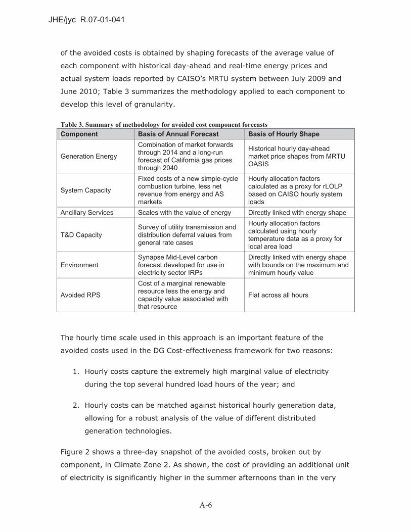
PageA-6
of the avoided costs is obtained by shaping forecasts of the average value of
each component with historical day-ahead and real-time energy prices and
actual system loads reported by CAISO’s MRTU system between July 2009 and
June 2010; Table 3 summarizes the methodology applied to each component to
develop this level of granularity.
Table 3. Summary of methodology for avoided cost component forecasts Component Basis of Annual Forecast Basis of Hourly Shape
Generation Energy
Combination of market forwards through 2014 and a long-run forecast of California gas prices through 2040
Historical hourly day-ahead market price shapes from MRTU OASIS
System Capacity
Fixed costs of a new simple-cycle combustion turbine, less net revenue from energy and AS markets
Hourly allocation factors calculated as a proxy for rLOLP based on CAISO hourly system loads
Ancillary Services Scales with the value of energy Directly linked with energy shape
T&D Capacity Survey of utility transmission and distribution deferral values from general rate cases
Hourly allocation factors calculated using hourly temperature data as a proxy for local area load
Environment Synapse Mid-Level carbon forecast developed for use in electricity sector IRPs
Directly linked with energy shape with bounds on the maximum and minimum hourly value
Avoided RPS
Cost of a marginal renewable resource less the energy and capacity value associated with that resource
Flat across all hours
The hourly time scale used in this approach is an important feature of the
avoided costs used in the DG Cost-effectiveness framework for two reasons:
1. Hourly costs capture the extremely high marginal value of electricity
during the top several hundred load hours of the year; and
2. Hourly costs can be matched against historical hourly generation data,
allowing for a robust analysis of the value of different distributed
generation technologies.
Figure 2 shows a three-day snapshot of the avoided costs, broken out by
component, in Climate Zone 2. As shown, the cost of providing an additional unit
of electricity is significantly higher in the summer afternoons than in the very
JHE/jyc R.07-01-041

PageA-7
early morning hours. This chart also shows the relative magnitude of different
components in this region in the summer for these days. The highest peaks of
total cost (over $1,000/MWh) are driven primarily by the allocation of generation
and T&D capacity to the highest load hours, but also by higher wholesale energy
prices during the middle of the day.
Figure 2. Three-day snapshot of energy values in CZ2
$0
$200
$400
$600
$800
$1,000
$1,200
$1,400
$1,600
Thu,�Aug13
Fri,�Aug�14 Sat,�Aug�15
Avoi
ded�
Cost
�($/M
Wh) T&D
Capacity
Emissions
Ancillary�Services
Losses
Avoided�RPS
Energy
Figure 3 shows average monthly value of load reductions, revealing the seasonal
characteristics of the avoided costs. The energy component dips in the spring,
reflecting increased hydro supplies and imports from the Northwest; and peaks
in the summer months when demand for electricity is highest. The value of
capacity—both generation and T&D—is concentrated in the summer months and
results in significantly more value on average in these months.
JHE/jyc R.07-01-041

PageA-8
Figure 3. Average monthly avoided cost (levelized value over 30-yr horizon)
$0
$50
$100
$150
$200
$250
Jan Feb Mar Apr May Jun Jul Aug Sep Oct Nov Dec
Aver
age�
Mon
thly
�Val
ue�o
f�Ene
rgy�
($/M
Wh)
T&D
Capacity
Emissions
Ancillary�Services
Losses
Energy
Avoided�RPS
Figure 4 shows the components of value for the highest value hours in sorted
order of cost. This chart shows the relative contribution to the highest hours of
the year by component. Note that most of the high cost hours occur in
approximately the top 200 to 400 hours—this is because most of the value
associated with capacity is concentrated in a limited number of hours. While the
timing and magnitude of these high costs differ by climate zone, the
concentration of value in the high load hours is a characteristic of the avoided
costs in all of California.
JHE/jyc R.07-01-041

PageA-9
Figure 4. Price duration curve showing top 1,000 hours for CZ2
$0
$500
$1,000
$1,500
$2,000
$2,500
$3,000
0 100 200 300 400 500 600 700 800 900 1000
Avoi
ded�
Cost
��($/
MW
h)
Top�1000�Hours
T&D
Capacity
Emissions
Ancillary�Services
Losses
Energy
Avoided�RPS
Generation Energy
The avoided cost of energy reflects the marginal cost of generation needed to
meet load in each hour. The forecast values of energy include short and long-run
components. The wholesale value of energy through 2014 is based on market
forwards for NP15 and SP15. The long-run value of energy is calculated based on
the assumption that the average market heat rate will remain stable; the implied
market heat rate based on 2014 forwards is extended through 2040. The long-
run value of energy is calculated by multiplying the monthly forecast of gas
prices in California by this market heat rate. The combined forecast is shown in
Figure 5.
Figure 5. Forecast of average wholesale energy price based on market forwards and gas forecast.
Market�Forwards Long�Run�Forecast
$0
$20
$40
$60
$80
$100
$120
$140
2010 2015 2020 2025 2030 2035 2040
Aver
age�
Who
lesa
le�E
nerg
y�Va
lue�
($/M
Wh)
JHE/jyc R.07-01-041
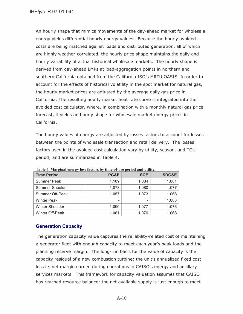
PageA-10
An hourly shape that mimics movements of the day-ahead market for wholesale
energy yields differential hourly energy values. Because the hourly avoided
costs are being matched against loads and distributed generation, all of which
are highly weather-correlated, the hourly price shape maintains the daily and
hourly variability of actual historical wholesale markets. The hourly shape is
derived from day-ahead LMPs at load-aggregation points in northern and
southern California obtained from the California ISO’s MRTU OASIS. In order to
account for the effects of historical volatility in the spot market for natural gas,
the hourly market prices are adjusted by the average daily gas price in
California. The resulting hourly market heat rate curve is integrated into the
avoided cost calculator, where, in combination with a monthly natural gas price
forecast, it yields an hourly shape for wholesale market energy prices in
California.
The hourly values of energy are adjusted by losses factors to account for losses
between the points of wholesale transaction and retail delivery. The losses
factors used in the avoided cost calculation vary by utility, season, and TOU
period; and are summarized in Table 4.
Table 4. Marginal energy loss factors by time-of-use period and utility. Time Period PG&E SCE SDG&E Summer Peak 1.109 1.084 1.081 Summer Shoulder 1.073 1.080 1.077 Summer Off-Peak 1.057 1.073 1.068 Winter Peak - - 1.083 Winter Shoulder 1.090 1.077 1.076 Winter Off-Peak 1.061 1.070 1.068
Generation Capacity
The generation capacity value captures the reliability-related cost of maintaining
a generator fleet with enough capacity to meet each year’s peak loads and the
planning reserve margin. The long-run basis for the value of capacity is the
capacity residual of a new combustion turbine: the unit’s annualized fixed cost
less its net margin earned during operations in CAISO’s energy and ancillary
services markets. This framework for capacity valuation assumes that CAISO
has reached resource balance: the net available supply is just enough to meet
JHE/jyc R.07-01-041
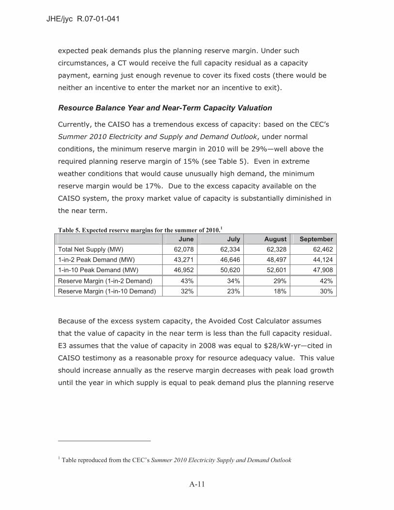
PageA-11
expected peak demands plus the planning reserve margin. Under such
circumstances, a CT would receive the full capacity residual as a capacity
payment, earning just enough revenue to cover its fixed costs (there would be
neither an incentive to enter the market nor an incentive to exit).
Resource Balance Year and Near-Term Capacity Valuation
Currently, the CAISO has a tremendous excess of capacity: based on the CEC’s
Summer 2010 Electricity and Supply and Demand Outlook, under normal
conditions, the minimum reserve margin in 2010 will be 29%—well above the
required planning reserve margin of 15% (see Table 5). Even in extreme
weather conditions that would cause unusually high demand, the minimum
reserve margin would be 17%. Due to the excess capacity available on the
CAISO system, the proxy market value of capacity is substantially diminished in
the near term.
Table 5. Expected reserve margins for the summer of 2010.1
June July August SeptemberTotal Net Supply (MW) 62,078 62,334 62,328 62,4621-in-2 Peak Demand (MW) 43,271 46,646 48,497 44,1241-in-10 Peak Demand (MW) 46,952 50,620 52,601 47,908
Reserve Margin (1-in-2 Demand) 43% 34% 29% 42%Reserve Margin (1-in-10 Demand) 32% 23% 18% 30%
Because of the excess system capacity, the Avoided Cost Calculator assumes
that the value of capacity in the near term is less than the full capacity residual.
E3 assumes that the value of capacity in 2008 was equal to $28/kW-yr—cited in
CAISO testimony as a reasonable proxy for resource adequacy value. This value
should increase annually as the reserve margin decreases with peak load growth
until the year in which supply is equal to peak demand plus the planning reserve
1 Table reproduced from the CEC’s Summer 2010 Electricity Supply and Demand Outlook
JHE/jyc R.07-01-041

PageA-12
margin—this is known as the resource balance year and is calculated to be 2015
(see Figure 6).2
Figure 6. Evaluation of resource balance year. Resource�Balance�
Year
0
10,000
20,000
30,000
40,000
50,000
60,000
70,000
80,000
90,000
2008 2012 2016 2020
Load
/Net
�Sup
ply
Non�OTC�Existing�Fleet OTC�Existing�Fleet
Dependable�Renewables Planned�Fossil�Additions
In the resource balance year and each year thereafter, the value of capacity is
equal to the full capacity residual. Between 2008 and the resource balance year,
E3 uses a linear interpolation to calculate the annual increases in capacity value.
The final forecast of capacity value is shown in Figure 7.
2 The resource balance year is evaluated by comparing the CEC's forecast of peak loads in California with California's expected committed capacity resources. The forecast for expected capacity includes several components: 1) existing system capacity as of 2008, net of expected plant retirements; 2) fossil plants included in the CEC's list of planned projects with statuses of "Operational," "Partially Operational," or " Under Construction"; and 3) a forecast of renewable capacity additions to the system that would be necessary to achieve California's 33% Renewable Portfolio Standard by 2020 based on E3's 33% Model.
JHE/jyc R.07-01-041

PageA-13
Figure 7. Forecast of capacity value included in avoided costs.
Short�Run�Value
Long�Run�Value�(Capacity�Residual)
$0
$20
$40
$60
$80
$100
$120
$140
$160
$180
$200
2010 2015 2020 2025 2030 2035 2040
Capa
city
�Val
ue�($
/kW
�yr)
Calculation of the Capacity Residual
The DG Cost-Effectiveness Framework calculates the capacity residual of the CT
for each year of the avoided cost series by dispatching a representative unit
against an hourly real-time market price curve and subtracting the net margin
from the unit’s annualized fixed costs. The hourly shape of the real-time market
is based on historical real-time data gathered from CAISO’s MRTU system; in
each year, the level of the real-time market price curve is adjusted to match the
average wholesale market price for that year. The CT’s net margin is calculated
assuming that the unit dispatches at full capacity in each hour that the real-time
price exceeds its operating cost (the sum of fuel costs and variable O&M) plus a
bid adder of 10%; in each hour that it operates, the unit earns the difference
between the market price and its operating costs. In each hour where the
market prices are below the operating cost, the unit is assumed to shut down.
The revenues earned through this economic dispatch are grossed up by 11% to
account for profits earned through participation in CAISO’s ancillary services
markets.3 The final figure is subtracted from the CT’s annualized fixed cost—
calculated using a pro-forma tool to amortize capital and fixed operations and
maintenance costs—to determine the CT residual in that year.
3 This figure is based on an analysis of new combustion turbine operations presented in the CAISO’s 2009 Market Report on Market Issues and Performance.
JHE/jyc R.07-01-041

PageA-14
CT Performance Adjustments
The CT’s rated heat rate and nameplate capacity characterize the unit’s
performance at ISO conditions,4 but the unit’s actual performance deviates
substantially from these ratings throughout the year. In California, deviations
from rated performance are due primarily to hourly variations in temperature.
Figure 8 shows the relationship between temperature and performance for a GE
LM6000 SPRINT gas turbine, a reasonable proxy for current CT technology.
Figure 8. Temperature-performance curve for a GE LM6000 SPRINT combustion turbine.
60%
70%
80%
90%
100%
110%
120%
0 20 40 60 80 100
Perc
ent�D
esig
n
Temperature�(°F)
Heat�Rate
Output
The effect of temperature on performance is incorporated into the calculation of
the CT residual; several performance corrections are considered:
� In the calculation of the CT’s dispatch, the heat rate is assumed to
vary on a monthly basis. In each month, E3 calculates an average
day-time temperature based on hourly temperature data throughout
the state and uses this value to adjust the heat rate—and thereby the
operating cost—within that month.
� Plant output is also assumed to vary on a monthly basis; the same
average day-time temperature is used to determine the correct
4 ISO conditions assume 59ºF, 60% relative humidity, and elevation at sea level.
JHE/jyc R.07-01-041

PageA-15
adjustment. This adjustment affects the revenue collected by the
plant in the real-time market. For instance, if the plant’s output is
90% of nameplate capacity in a given month, its net revenues will
equal 90% of what it would have received had it been able to operate
at nameplate capacity.
� The resulting capacity residual is originally calculated as the value per
nameplate kilowatt—however, during the peak periods during which a
CT is necessary for resource adequacy, high temperatures will result in
a significant capacity derate. Consequently, the value of capacity is
increased by approximately 9% to reflect the plant’s reduced output
during the top 250 load hours of the year as shown in Figure 9.
Figure 9. Adjustment of capacity value to account for temperature derating during periods of peak load.
$0
$20
$40
$60
$80
$100
$120
$140
$160
$180
$200
2008
2010
2015
2020
2025
2030
2035
2040
Capa
city
�Val
ue�($
/kW
�yr)
Based�on�Rated�Output
Based�on�Temperature�Corrected�Output
Other Adjustments to the Capacity Residual
The valuation of capacity includes an adjustment for losses between point of
generation and delivery similar to energy. In order to account for losses, the
annual capacity value is multiplied by the utility-specific losses factor applicable
to the summer peak period, as this is the period during which system capacity is
likely to be constrained.
Additionally, the Avoided Cost Calculator includes a discretionary adjustment for
reductions in the planning reserve margin. Resources that are used to meet the
planning reserve margin receive 100% of the value of capacity; resources that
JHE/jyc R.07-01-041

PageA-16
reduce the forecast of peak load and the planning reserve margin receive 115%
of the value of capacity. Whether this adjustment should be included varies on a
resource-by-resource basis and should be carefully considered.
Hourly Allocation of Capacity Value
The Avoided Cost Calculator bases its allocation of capacity value to a subset of
hours upon hourly system load data collected from January 2006 through June
2010. In each full calendar year, hourly allocators are calculated for that year’s
top 250 load hours; the allocators, which sum to 100% within each year, are
inversely proportional to the difference between the annual peak plus operating
reserves and the loads in each hour. This allocation methodology, which serves
as a simplified and transparent proxy for models of relative loss-of-load
probability (rLOLP), results in allocators that increase with the load level.
The annual series of allocators for each of the full calendar years are used to
develop reasonable estimates of the relative fraction of capacity value that is
captured within each month as shown in Figure 10. By considering loads within
the four-year period from 2006-2009, the Avoided Cost Calculator captures the
potential diversity of peak loads across different years.
Figure 10. Calculation of monthly capacity allocation based on historical data from 2006-2009.
0%
10%
20%
30%
40%
50%
60%
70%
80%
Jan Feb Mar Apr May Jun Jul Aug Sep Oct Nov Dec
Mon
thly
�Allo
catio
n�of
�Cap
acity
�Val
ue
Average2006200720082009
JHE/jyc R.07-01-041

PageA-17
Table 6. Summary of monthly capacity allocation based on historical load data from 2006-2009.
Month Capacity
Allocation(%)
Number of Constrained
Hours January 0.0% 0 February 0.0% 0 March 0.0% 0 April 0.0% 0 May 0.9% 2 June 8.8% 22 July 40.2% 100 August 31.8% 80 September 17.8% 45 October 0.5% 1 November 0.0% 0 December 0.0% 0 Total 100.0% 250
Hourly allocators based on CAISO system loads from July 2009 through June
2010 are calculated using the historical monthly allocation of capacity. The
algorithm used to allocate the value of capacity to hours within this calendar
year parallels the process used for the historical analysis but shifts the time scale
from allocation across an entire year to allocation within single months. Thus,
for each month between July 2009 and June 2010, the value of capacity is
allocated to the number of constrained hours in that month so that the allocators
sum to the total monthly allocation shown in Table 6. As with the historical
analysis, the allocators are inversely proportional to the difference between the
month’s peak load plus operating reserves and the load in the relevant hour.
JHE/jyc R.07-01-041

PageA-18
Figure 11. Hourly allocation of generation capacity based on loads from July 2009 through June 2010.
Ancillary Services (A/S)
Besides reducing the cost of wholesale purchases, reductions in demand at
the meter result in additional value from the associated reduction in required
procurement of ancillary services. The CAISO MRTU markets include four
types of ancillary services: regulation up and down, spinning reserves, and
non-spinning reserves. The procurement of regulation services is generally
independent of load; consequently, behind-the-meter load reductions and
distributed generation exports will not affect their procurement. However,
both spinning and non-spinning reserves are directly linked to load—in
accordance with WECC reliability standards, the California ISO must maintain
an operating reserve equal to 5% of load served by hydro generators and
7% of load served by thermal generators.
As a result, load reductions do result in a reduction in the procurement of
reserves; the value of this reduced procurement is included as a value
stream in the Avoided Cost Calculator. It is assumed that the value of
avoided reserves procurement scales with the value of energy in each hour
throughout the year. According to the CAISO’s 2009 Annual Report on
Market Issues and Performance, total spending on reserves in 2009
JHE/jyc R.07-01-041

PageA-19
amounted to 1.0% of the value of total wholesale purchases. E3 uses this
figure to assess the value of avoided reserves procurement in each hour.
T&D Capacity
The avoided costs include the value of the potential deferral of transmission and
distribution network upgrades that could result from reductions in local peak
loads. The marginal value of T&D deferral is highly location-specific; E3 has
gathered utility data on utility T&D investment plans and computed the cost of
planned T&D investments on a $/kW-yr basis. Synthesizing data gathered from
general rate cases of the three major IOUs, E3 has calculated statewide average
deferral values for both transmission and distribution infrastructure. As with
generation energy and capacity, the value of deferring transmission and
distribution investments is adjusted for losses during the peak period using the
factors shown in Table 7. These factors are lower than the energy and capacity
adjustments because they represent losses from transmission and distribution
voltage levels to the retail delivery point.
Table 7. Losses factors for transmission and distribution capacity. PG&E SCE SDG&E
Distribution 1.048 1.022 1.043 Transmission 1.083 1.054 1.071 The network constraints of a distribution system must be satisfactory to
accommodate the area’s local peaks; accordingly, the Avoided Cost Calculator
allocates the deferral value in each zone to the hours of the year during which
the system is most likely to be constrained and require upgrades—the hours of
highest local load. Because local loads were not readily available for this
analysis, hourly temperatures were used as a proxy to develop allocation factors
for T&D value, a methodology that has been benchmarked against actual local
load data and was originally developed for the E3 Calculator used to evaluate the
benefits of utility energy efficiency programs. This approach results in an
allocation of T&D value to several hundred of the hottest — and likely highest
local load — hours of the year (Figure 12). Figure 13 shows the total allocation of
T&D within each month for each of the climate zones. Different weather patterns
throughout the state result in unique allocators for T&D capacity.
JHE/jyc R.07-01-041
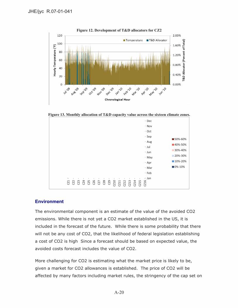
PageA-20
Figure 12. Development of T&D allocators for CZ2
Figure 13. Monthly allocation of T&D capacity value across the sixteen climate zones.
Jan
Feb
Mar
Apr
May
Jun
Jul
Aug
Sep
Oct
Nov
Dec
CZ1
CZ2
CZ3
CZ4
CZ5
CZ6
CZ7
CZ8
CZ9
CZ10
CZ11
CZ12
CZ13
CZ14
CZ15
CZ16
50%�60%
40%�50%
30%�40%
20%�30%
10%�20%
0%�10%
Environment
The environmental component is an estimate of the value of the avoided CO2
emissions. While there is not yet a CO2 market established in the US, it is
included in the forecast of the future. While there is some probability that there
will not be any cost of CO2, that the likelihood of federal legislation establishing
a cost of CO2 is high Since a forecast should be based on expected value, the
avoided costs forecast includes the value of CO2.
More challenging for CO2 is estimating what the market price is likely to be,
given a market for CO2 allowances is established. The price of CO2 will be
affected by many factors including market rules, the stringency of the cap set on
JHE/jyc R.07-01-041

PageA-21
CO2 allowances, and other elements. The DG Cost-effectiveness Framework
uses a forecast developed by Synapse Consulting through a meta-analysis of
various studies of proposed climate legislation. The mid-level forecast included
in this report was developed explicitly for use in electricity sector integrated
resource planning and so serves as an appropriate applied value for the cost of
carbon dioxide emissions in the future.
Assuming that natural gas is the marginal fuel in all hours, the hourly emissions
rate of the marginal generator is calculated based on the day-ahead market price
curve. The link between higher market prices and higher emissions rates is
intuitive: higher market prices enable lower-efficiency generators to operate,
resulting in increased rates of emissions at the margin. Of course, this
relationship holds for a reasonable range of prices but breaks down when prices
are extremely high or low. For this reason, the avoided cost methodology
bounds the maximum and minimum emissions rates based on the range of heat
rates of gas turbine technologies. The maximum and minimum emissions rates
are bounded by a range of heat rates for proxy natural gas plants shown in Table
8; the hourly emissions rates derived from this process are shown in Figure 14.
Table 8. Bounds on electric sector carbon emissions.
Proxy Low Efficiency Plant
Proxy High Efficiency Plant
Heat Rate (Btu/kWh) 12,500 6,900 Emissions Rate (tons/MWh) 0.731 0.404
JHE/jyc R.07-01-041

PageA-22
Figure 14. Hourly emissions rates derived from market prices (hourly values shown in descending order).
Market�Heat�Rate Implied�Emissions�Rate
0.00
0.23
0.47
0.70
0.94
1.17
0
4,000
8,000
12,000
16,000
20,000
tons
/MW
h
kBtu
/MW
h
Hour�(Descending�Order)
Avoided Renewable Purchases
The DG Cost-effectiveness Framework also includes the value of avoided
renewable purchases. Because of California's commitment to reach a RPS
portfolio of 33% of total retail sales by 2020, any reductions to total retail sales
will result in an additional benefit by reducing the required procurement of
renewable energy to achieve RPS compliance. This benefit is captured in the
avoided costs through the RPS Adder.
The calculation of benefits resulting from avoided purchases of renewables
begins in 2020. Because of the large gap between existing renewable resources
and the 33% target in 2020, the rate of renewable procurement up until this
year is unlikely to change with small reductions to the total retail load. However,
after 2020, any reduction to retail sales will reduce requirements to obtain
additional resources to continue compliance with the 33% case. As a result, the
value of avoided renewable purchases is considered a benefit associated with
load reductions beyond 2020.
The RPS Adder is a function of the Renewable Premium, the incremental cost of
the marginal renewable resource above the cost of conventional generation. The
JHE/jyc R.07-01-041

PageA-23
marginal renewable resource is based upon the Fairmont CREZ, the most
expensive resource bundle that is included in the renewable portfolio in E3's 33%
Model 33% Reference Case. The Renewable Premium is calculated by subtracting
the market energy and capacity value associated with this bundle, as well as the
average CO2 emissions from a CCGT, from its levelized cost of energy as shown
below. The RPS Adder is calculated directly from the Renewable Premium by
multiplying by 33%, as, for each 1 kWh of avoided retail sales, 0.33 kWh of
renewable purchases are avoided.
Figure 15. Evaluation of the Renewable Premium
$0
$50
$100
$150
$200
$250
2020 2024 2028 2032 2036 2040
$/M
Wh
Energy�ValueEmissions�ValueCapacity�ValueRenewable�PremiumRenewable�Cost
Key Data Sources and Specific Methodology
This section provides further discussion of data sources and methods used in the
calculation of the hourly avoided costs.
Natural gas forecast
The natural gas price forecast, which is the basis for the calculation of the CCGT
all-in cost, is based upon from the CPUC MPR 2009 Update. This forecast is
based upon NYMEX Henry Hub futures, average basis differentials, and delivery
charges to utilities. The forecast is shown in Figure 16. The MPR’s forecast
methodology has been expanded to incorporate expected monthly trends in gas
prices—commodity prices tend to rise in the winter when demand for gas as a
JHE/jyc R.07-01-041
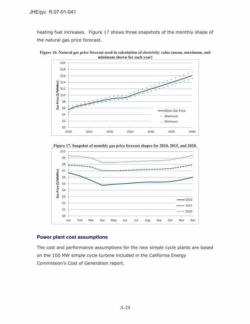
PageA-24
heating fuel increases. Figure 17 shows three snapshots of the monthly shape of
the natural gas price forecast.
Figure 16. Natural gas price forecast used in calculation of electricity value (mean, maximum, and minimum shown for each year)
$0
$2
$4
$6
$8
$10
$12
$14
$16
$18
$20
2010 2015 2020 2025 2030 2035 2040
Gas
�Pric
e�($
/MM
Btu)
Mean�Gas�Price
Maximum
Minimum
Figure 17. Snapshot of monthly gas price forecast shapes for 2010, 2015, and 2020.
$0
$1
$2
$3
$4
$5
$6
$7
$8
$9
$10
Jan Feb Mar Apr May Jun Jul Aug Sep Oct Nov Dec
Gas
�Pric
e�($
/MM
Btu)
2010
2015
2020
Power plant cost assumptions
The cost and performance assumptions for the new simple cycle plants are based
on the 100 MW simple cycle turbine included in the California Energy
Commission’s Cost of Generation report.
JHE/jyc R.07-01-041

PageA-25
Table 9. Power plant cost and performance assumptions (all costs in 2009 $) Simple Cycle Gas
Turbine Heat Rate (Btu/kWh) 9,300 Plant Lifetime (yrs) 20 Instant Cost ($/kW) $1,230 Fixed O&M ($/kW-yr) $17.40 Variable O&M ($/kW-yr) $4.17 Debt-Equity Ratio 60% Debt Cost 7.70% Equity Cost 11.96%
Cost of CO2 Emissions
The CO2 cost projection is taken from a meta-analysis of CO2 price forecasts.
Figure 18 summarizes the Synapse price forecasts; the mid-level forecast is used
in the calculation of avoided costs.
Figure 18. The CO2 price series embedded in the avoided cost values
$0
$20
$40
$60
$80
$100
$120
2010 2015 2020 2025 2030 2035 2040
Carb
on�P
rice�
(nom
inal
�$/t
onne
)
Synapse�Low�Forecast
Synapse High�Forecast
Synapse Mid�Forecast�(Used�in�Avoided�Costs)
The marginal rate of carbon emissions is interpolated from the hourly value of
energy assuming that the marginal generator burns natural gas in all hours.
JHE/jyc R.07-01-041

PageA-26
Calculation of the System Capacity Allocators
The following calculation sequence is used to compute a capacity cost allocation
factor in each of the top 250 system load hours. This methodology is applied in
the calculation of the hourly avoided cost of electricity:
1. Compute the system capacity that provides 7% operating reserves = peak
load * 1.07
2. Compute a relative weight in each hour as the reciprocal of the difference
between the load in each of the top 250 hours and the planned system
capacity
3. Normalize the weights in each hour to sum to 100%
Calculation of the T&D Capacity Allocators
The following is a brief description of the algorithm used to allocated T&D
capacity value. T&D capacity value is allocated to all hours with temperatures
within 15ºF of the peak annual temperature.
1. Select all hours with temperatures within 15ºF of the peak annual
temperature (excluding hours on Sundays and holidays) and order them
in descending order
2. Assign each hour an initial weight using a triangular algorithm, such that
the first hour (with the highest temperature) has a weight of 2/(n+1) and
the weight assigned to each subsequent hour decreases by 2/[n*(n+1)],
where n is the number of hours that have a temperature above the
threshold established in the first step
3. Average the initial weights among all hours with identical temperatures so
that hours with the same temperature receive the same weight
JHE/jyc R.07-01-041
APPENDIX B:
STAKEHOLDER FEEDBACK
��
�
JHE/jyc R.07-01-041

PageB-2
Appendix B: Stakeholder Feedback
Please note that the following views are those of the interviewees or industry
stakeholders who submitted feedback, and not necessarily views of E3 or
StrateGen. In addition, they are summaries, and are not an exhaustive list of all
feedback provided.
Interview Summary Notes
IOUs
SDG&E
� Would have liked less money for marketing and more for implementation
� Like the idea of payment milestones, but they need to be simple to reduce
administrative costs
� Refrigeration is tricky: some customers had to change their business
model because of the economy (i.e., what they store), at which point PLS
is no longer a viable option
� Currently a large part of the program is fuel switching, which may not be
an option in the current definition
SCE
� Need a rate that provides a sustainable payback, and a guarantee that the
rate structure will stay in place. One option might include a 10 year PLS
tariff, or a guarantee for as long as the standard offer is available.
� However, a rate is not enough – only a handful of engineers understand
the market, which is a big issue
� A lot of challenges with Honeywell because of technology expense and
engineering challenges
JHE/jyc R.07-01-041

PageB-3
PG&E
� Smaller systems seemed more difficult to sell, even with higher
incentives. As a result, Cypress has experienced challenges selling the
smaller capacity systems it was limited to in its original contract, which is
why the Cypress contract was recently expanded to include additional
technologies.
� It has been an onerous process for both sides to track performance for
incentive payments.
Pilot Vendors:
Honeywell
� Significant implementation challenges: weight of unit led to structural
engineering costs, which were not covered in the incentives; schools had
DSA requirements; limited # of contractors to do install
� Existing customers seem very satisfied with unit, and actual is close to
estimated shift, and no maintenance issues
� Targeting customers was a big issue: would be helpful to work with SCE
to target customers with the correct rate structure
� Tried to run education/training for contractors, but payback wasn't good
enough and most lost interest
� Either need a very high incentive (the current incentive is just not good
enough), or a lower incentive and new rate
Cypress
� PG&E direct access requirement was very challenging; would want all
customers allowed to participate
� Significant implementation issues: weight/structural engineering, DSA
requirements, expense
JHE/jyc R.07-01-041

PageB-4
� PG&E monitoring requirements were very complex and added to cost;
energy neutrality requirements made the program even more complex,
and seems out of scope of PLS
� PG&E rebate structure with persistence payments made it too complex
and a deterrent to customers – need to focus more on customer education
� With SCE, no problem getting fully subscribed, but had to bundle because
of low rebate – need a higher rebate to truly drive demand
� Refurbishment of TES units is cost effective, potential for a lot of projects
� TES and gas cooling is too complex for a standard offer
� For incentives, $500/kW is bottom limit, $750 is “sweet spot.” Also, need
certainty in rates. Would recommend a traditional utility program, then
when market grows go to standard offer + TOU.
� Lack of education/training in design community is a huge issue.
Trane
� Implementation challenges: weight, DSA, expensive (even at $2000/kW,
15 year payback)
� Generally targeted old units that needed replacement and new
construction, to get around above issues
� Could probably get by with a $1000-$1200/kW incentive without energy
neutrality (~$200 more with energy neutrality)
� RFP process seemed to work well. A standard offer would be challenging
because of the range in technologies. Rate needs more certainty.
� interested in a voluntary special tariff for PLS customers
� Challenges getting baseline data
JHE/jyc R.07-01-041

PageB-5
Retrofit Originality Inc.
� Should focus on PLS and EE; otherwise allows for poor design. With CAC,
very successful in doing EE and PLS.
� A lot of units that aren't running optimally. Would be cost effective to go
and fine tune these systems.
� Would recommend combination of utility rates, tax incentives, and
rebates, because a program needs some owner incentive
� Needs to be a 3 year payback for commercial ($1300/kW won't get you
far because its a 10 year payback)
� Likes idea of a graduated incentive that incorporates EE
� Training is a huge deal...need more training, performance-based
commissioning.
EPS
� Joint vendor-IOU effort in targeting customers would be much more
effective
� Many more potential customers than served in the program – potential for
expansion
� Some challenges in customer scheduling or customer equipment issues
(not related to EPS technology)
� In a future program, would need additional funds for marketing
� Challenges because of economy: baseline dropped (so didn't get projected
demand savings) and some installations were no longer able to load shift
due to changing product profile
� Additional flexibility in terms of shifting window would lead to additional
benefits
JHE/jyc R.07-01-041

PageB-6
� Facility related off-peak demand charge could be a big deterrent.
� Ice manufacturing is an ideal candidate for EPS technology: a perfect fit in
terms of climate, product type, ability to process shift unloading of
product
Other:
Klaus Schiess (KS Engineering)
� A guaranteed rate is essential...need better rate structure to incent, at
which point there is no need for a rebate.
� Training and educational tools are also essential
� A lot of existing systems could be fine tuned
� Need more quality control in feasibility studies
� Wants to expand COOLAID
Cogent
� Minimum threshold for incentive level: 5-7 year for public, 2-3 private
� For incentive, 50% at application and 50% at the completion would be
ideal. Combined TOU differential and demand charge would also be good.
� For technologies, ice is “more forgiving” but investment is not as good.
Chilled water is challenging because of operating differential
ASW
� Very challenging to get baseline data in order to measure performance
� No one will buy unless it's less than a 5 year payback, so batteries are
very challenging (have found 20+ year payback)
� Ice storage seems to require more knowledge than the typical operator
has. Also, smaller ice systems seem very challenging and too expensive.
JHE/jyc R.07-01-041

PageB-7
� Have to have certainty in rates, and incentive should be paid out over 5
years and based on performance
� Majority of systems not working at full capacity – a lot of potential to fix
systems
Ken Gillespie (PG&E)
� Key benefit is reducing ampacity at the meter
� Improving delta T for chilled water is essential
� Smaller ice systems can be challenging due to maintenance issues. Fr
example, the facility owner might not understand how to maintain glycol
levels.
� Lack of training/education is a huge issue
Transphase
� Technology neutral is a good thing
� EM&V was overly complex...added a lot of additional costs/effort ($40-
50k)
� Any program should be heavily performance-based
� With a more favorable rate schedule, a standard offer might be
unnecessary
� Prefers market value oriented approach, where the value of shifting a kW
should be the same and thus receive the same incentive
� There would be challenges in a residential market – no economies of
scale, and the education aspect would be a huge burden
� Maintenance costs were negligible – found customers using systems after
20 years w/ few problems
JHE/jyc R.07-01-041

PageB-8
� For energy efficiency, should look at site vs. source energy, including heat
rates of the power plants. In theory, avoided costs should reflect heat
rates and cost of production, rates should reflect avoided costs.
Schneider Electric
� Generally a 2 year payback is necessary. Some industries, such as
pharmaceuticals, might tolerate longer paybacks like 7 years. At 10+
years, this is definitely too much risk.
� Waste water treatment plants may be a good target
� Has encountered a lot of rate change fear
� Equipment: most facilities will not want to purchase bigger equipment
that would allow them to shut off during the day and turn on at night
Cristopia
� Feasibility studies were not done well, due to engineer lack of tracking
� Challenge in marketing – building owners don't care about load shift
because the savings are passed on. Better in buildings where owner is
tied to costs.
� Need a sustainable business model, which means changing rate structure
� There are opportunities to process shift across the system, but no one
would bother because of rate structure
SCPPA
� Customers are unwilling to make investment because of TOU risk
� Huge cost advantages to doing high volume – primary incentive for utility-
owned model, but also good for society
� Equipment maintenance responsibilities vary widely, so can be complex
JHE/jyc R.07-01-041

PageB-9
� Utility doesn't want to deal with O&M call, so set up a call center
� Pre and post-installation analysis is very challenging
Invensys
� Establishing baseline for some processes – such as batch processes – will
be more challenging for industrial facilities than in buildings
� Liquid processes (water utilities, etc.) may be good candidates for process
shifting, as well as paper mills
� 2-3 year payback (1 in the recession) necessary, although “green” focus
can shift this somewhat
Enovity
� Need customized sequences to get value, which should be done building
by building
� At low loads, it is better to run the tank because the chiller does not run
very efficiently at low load and one can also avoid start and stop problems
from an under-loaded chiller.
� Big issue – some customers opt out of energy purchasing, with a fixed
$/kWh rate 24/7 from provider. With the inefficiencies of running a TES
system (compared to chilled water plant), this becomes more expensive,
and the customer would save money by not using the system
Davis Energy Group
� Precooling – need an efficient envelope in order to store cooling
� If a building can tolerate 8-10 degree float, can do a lot with precooling
(but many people are unwilling to tolerate any change in service)
JHE/jyc R.07-01-041

PageB-10
� Much easier to work with new construction, as you can plan for space and
existing construction tends to be poor
� Rate structures don't reflect the peak load problems
� “Green” marketing might be effective
� Good to see how people are going to interact with the system before
going in
Glendale
� Targeting government buildings
� People tend to assume that the PLS technology is to blame when
something goes wrong, but typically it has been an issue with some other
equipment
� Biggest challenge has been dealing with building owners. Need to sit down
and educate them, which can be time consuming but effective
� Utility-ownership seems to be working very well
FPL
� Very cost effective to work with the design community...then you don't
need to target specific projects, as they will often know of a number of
eligible projects. Cuts down on marketing costs.
� Their program targets a 4-6 year payback, which is not enough for many
customers, who want a 2-3 year payback
� A lot of efficiencies in dealing with government/schools. For example,
there may be a number of buildings that can all be done at once.
� Had some customers who wanted to participate for environmental
reasons, but most are interested in saving money
JHE/jyc R.07-01-041

PageB-11
� TES has worked really well under current rate design (summer window:
12pm-9pm), but many customers have requested to shorten that window,
so created seasonal demand rate from 3-6. Now can design smaller
systems to shift for 3 hours – much more economical.
� Very important to shorten this window, and to create a rate just for TES.
� Need bill analysis, engineer sign off...feasibility study is very important
� 5 year learning curve (but may be quicker with technology today) – just
need to stick with it in terms of training
� Recommend: want to deal with customers that have qualified technician –
not just a lightbulb changer. Also – need to reach out to the customers
who are cutting edge. Though it is proven technology, it is a new
application for them.
Ice Energy
� Rate structure is a huge issue
� Limited to direct access customers – very challenging to subscribe
program
� Utility ownership models work well
� Standardization/consistency is extremely valuable in any program
structure
Workshop Feedback Summary Notes
Complete versions of feedback received are available at this link:
http://www.ethree.com/public_projects/sce1.html. Please note the feedback has
been edited to remove confidential information or specific company names where
necessary.
JHE/jyc R.07-01-041

PageB-12
Klaus Schiess, KSEngineers
� The report would benefit from a deadline extension and an additional
workshop
� The only way to achieve PLS goals is a rate that reflects real time pricing
or a TOU rate. If the rates alone do not achieve these goals, then other
incentives have to be offered.
� The analysis uses examples from the pilot projects, but these projects do
not represent the experience of TES as a whole
� TRC evaluation should not have any influence on the decision to have a
PLS program or not
� The concept that California has sufficient capacity until 2015 should not
have any influence on the decision making process
Paul Valenta/Mark MacCracken/Terry Andrews, Calmac
� Properly designed partial storage systems (vs. full storage) using ice
operate more efficiently, require less space, require fewer incremental
costs, while having better life cycle values, a lower connected load and
requiring less ratepayer funding.
� More information is necessary on how projects were selected for the
analysis
� Incremental costs in the report may not be accurate, and a 15 year life-
cycle is not accurate for a Calmac system
� Other PLS programs should be studied to determine specifically why they
do or do not work
JHE/jyc R.07-01-041

PageB-13
C. Clark, BG&E
� BG&E, along with several TES equipment manufacturers, presented
several educational seminars with large customers and consulting
engineers. Results were positive.
� If projects are designed to take advantage of all the tools that ice offers,
the initial system cost is often less than a conventional system of the
same capacity, and can result in a two to three year payback.
� Designs that take a conventional chiller system and add ice storage can
result in a six to eight year payback.
� When ice storage systems are compared to conventional systems,
generally only the cost of the ice and chiller are compared to the chiller
cost of a conventional system, which does not include other relevant cost
savings such as overall downsizing.
Scot Duncan, Retrofit Originality Inc.
� Utilities have a fiduciary responsibility to their shareholders to provide a
return on their investment, and installing PLS technologies can be counter
to this responsibility. If the utilities were able to include properly designed
and deployed PLS systems in their asset base, there would be a large
demand by utilities to deploy these technologies.
� Energy efficiency and performance monitoring are very important when
upgrading an existing TES or upgrading a non-TES to a TES system.
Otherwise poor operating strategies go unknown, and substantial energy
waste occurs.
� The monitoring requirement could be a part of the feasibility study.
� Adequate rate structures are needed not only to get TES in place but to
maintain optimal operation.
JHE/jyc R.07-01-041

PageB-14
� TES tanks in a chilled water storage application last far longer than 15
years
� Building power plants is extremely difficult and expensive, due to
regulations. It is unrealistic to estimate the actual cost of building
something that may not be able to get permitted or built in the actual
quantities that will need to get built for future growth and replacement of
existing capacity that may get retired.
� TES systems can range from energy neutral at the site to site energy
efficiency improvements of over 45%
John Andrepont, The Cool Solutions Company
� The analysis should be employing lower installed capital costs for medium
to large-scale TES installations
� New construction or retrofit capacity expansions can often be
economically justified without utility cash incentives.
� To capture a larger market penetration by TES, utility incentives would
play a major role in providing the necessary economic incentive to the
owners.
Stephen Clarke, AIC and East Penn Manufacturing
� TES is over represented in the analysis, which may bias program design.
Immediate availability of cost effective battery based systems appears to
be poorly understood by those involved in the generation, distribution and
regulation of electricity.
� The biggest barriers are 1) the lack of TOU pricing at the customer side of
the meter and 2) certainty that PLS system deployment will not be
hindered directly or indirectly by service providers.
� Incentives other than meaningful TOU price signals are not required and
should be a low priority.
JHE/jyc R.07-01-041

PageB-15
� Any PLS program must be technology-neutral
� Process Shifting requires nothing other than TOU pricing differentials
� If anything, residential customer based storage should be prioritized since
a) the other classes represent systems of a scale that could be provided
under other programs and initiatives, and b) domestic scale storage, if
implemented cost effectively, would potentially have the largest beneficial
impact.
� A standard offer matched with TOU pricing based incentives will drive
broad adoption of standardized packaged systems, maximizing cost,
reliability and service utility
� RFP based systems tend to become dominated by players with existing
RFP departments, and are typically not those organizations who exist to
develop viable PLS systems and technologies.
� We should be looking to incentivize standardized and packaged systems,
which do not require a feasibility study.
Doug Ames, Transphase
� Total capital cost from the utilities’ pilots were exaggerated compared to
normal installation costs
� Each installation should include a feasibility study, as well as pass a TRC
test
� A cost-based approach conflicts with a technology-neutral approach, and
provides impetus for manufacturers' costs to remain high. It also may be
unconstitutional.
SDG&E
� TES and non-TES categories should not be split any further without
compelling reason
JHE/jyc R.07-01-041

PageB-16
� Process shifting should be included in a standard offer or RFP
� Commercial, industrial, and public sector should be prioritized over
residential customer classes for now
� A standard offer is preferred, perhaps with 3-5 year contracts
� TOU energy benefits are modest and therefore persistence may be an
issue
� Operational savings are somewhat customer specific based on their load
profile. The ability to mitigate customer inconvenience will be what drives
adoption, with greater inconvenience requiring greater incentives.
� TOU operational savings combined with a one-time (or short term)
incentive to cover technology upgrades should be sufficient.
� The tariff structure should be utility specific
� A feasibility study seems reasonable, and could be included in a
Technology Audit (TA).
AES
� PLS provides social and private benefits, yet often private operating cost
savings do not offset the cost of implementing TES to the end-user.
� Social benefits often offset the implementation costs, especially for larger
projects. Thus, incentives are necessary and desirable to promote TES.
� AES supports a program that seeks to exploit the less costly projects first
and consider the usefulness and effectiveness of smaller projects
thereafter, which will naturally occur if incentive levels are equal.
� Standard offer is superior to RFP. The combination of higher transaction
costs for an RFP process and the timing mismatch with building owners
would result in higher costs for projects that are implemented.
JHE/jyc R.07-01-041

PageB-17
� An RFP is limiting: a host of other technologies, vendors, and
opportunities are eliminated from the field for the duration of the RFP.
� End-users focus on three issues: economic viability, managing
uncertainty, and ongoing involvement through monitoring and verification.
The cost/benefit equation must overcome the sum of these factors.
� In order to simplify an incentive program, shift calculations could be
based on efficiencies according to existing chiller age, in three categories:
older than 20 years, 11 to 20 years, and younger than 11 years.
� AES would support incentive levels between $1500 and $2000/kW given
current tariff structures
� It may be appropriate to eliminate off-peak demand charges for all
customers, rather than single out TES. On-peak demand charges could be
increased to meet revenue neutrality requirements.
� Rate certainty is important (perhaps 5 years for private sector and 10
years for public sector)
� A feasibility study would be a low-cost, effective tool for a PLS program
� The RIM test needs to be either modified or de-emphasized.
� Even if California has excess capacity through 2015, this should not stall
program implementation
� If separate financing were available for TES projects, they would not need
to compete with other projects for limited capital. Attempts to use utility
rate base financing would probably entail complications that would make
it unappealing.
JHE/jyc R.07-01-041

PageB-18
Feedback on Costs Following Workshop
Three stakeholders provided formal feedback on costs of thermal systems,
following the workshop: Doug Ames (Transphase), Cool Solutions and CB&I.
Due to the length of the Transphase response, we refer the reader to the full
document on the website, which is named “Install Costs Per kW Transphase-SCE
PSA.pdf”. (see this link: http://www.ethree.com/public_projects/sce1.html)
The Cool Solutions and CB&I feedback is provided below.
JHE/jyc R.07-01-041

PageB-19
TES�Project�Data�and�Capital�CostJ.S.�Andrepont���The�Cool�Solutions�Company���15��Nov���10
Approx.TES TES Peak Peak TES�Tank TES�ProjectInitial Load�Shift TES Cooling Electric Installed InstalledOperation Amount Capacity Load�Shift Load�Shift Cost Total�Cost(year) Application�Type State TES�Type (%�of�peak) (ton�hrs) (tons) (kW) ($�x�10^6) ($�x�10^6)
2003 District�Cooling FL chilled�water near�100% 160,000����� 20,000������� 15,000�������� 2.782���������� 8.0��������������1990 Corporate�R&D MI chilled�water 38% 68,000�������� 7,000���������� 5,250���������� 2.566���������� 5.2��������������2011 University�Campus IL chilled�water 29% 50,000�������� 9,750���������� 7,508���������� 3.767���������� 5.6��������������1993 University�Campus WA chilled�water partial 17,750�������� 2,536���������� 2,092���������� 1.200���������� 2.5��������������2002 Airport TX LoTempFluid near�100% 90,000�������� 30,000������� 21,000�������� 2.800���������� 10.0������������2004�2007 University�Campus AZ Ice partial 24,000�������� 3,000���������� 2,250���������� n.a. 4.2��������������
Net�CapitalSavings
TES Total�cost Total� Utility after�CreditInitial per�ton�hr TES�Project DSM for�SmallerOperation Unit�Cost Incentive Chiller�Plt(year) Application�Type State $/ton�hr ($/kW) ($/kW) ($�x�10^6)
2003 District�Cooling FL 50.0������������ 533�������������� none over�5.01990 Corporate�R&D MI 76.8������������ 994�������������� none 3.6���������������2011 University�Campus IL 111.8���������� 745�������������� none 2.4���������������1993 University�Campus WA 140.8���������� 1,195���������� none 1.5���������������2002 Airport TX 111.1���������� 476�������������� none 6.0���������������2004�2007 University�Campus AZ 176.0���������� 1,878���������� n.a. n.a.
Additional�Notes�on�Costs,�per�correspondence�with�Cool�Solutions�Co.:�����Above�are�for�above�grade�tanks.�The�"TES�Tank�Installated�cost"�would�be�roughly�double�for�an�undeground�tank.�����(Based�on�this�assumption,�the�$/ton�hour�costs�range�from�~�$70/Ton�hr�to�$200/Ton�hr�and�~�$600/kW�to�$1500/kW)��� As�projects�get�bigger,�economies�of�scale�result.�Smaller�systems�tend�(such�as�for�a�1,000�ton�hr�application)�are�more�typically�ice.��� Chilled�water�systems�especially�get�economies�of�scale�because�there�are�a�number�of�fixed�costs,�independent�of�size.����Costs�vary�greatly�due�to�a�number�of�factors,�such�as�union/non�union,�above/below�ground�.�� Ice�systems�tend�to�be�more�modular,�so�the�$/ton�hr�do�not�vary�as�much�
Additional�feedback�on�costs�and�program�design:�New�construction/�expansion�vs.�pure�retrofit:��� New�construction�and�expansions�do�not�often�need�rebates.�With�expansions,�existing�chiller�capacity�can�be�used�for����������the�expansion�(instead�of�installing�new�chillers)��� It is�hard�to�tap�into�pure�retrofit�market�without�DSM�incentivesOn�operational�challenges:���� With�larger�systems,�they�have�not�encountered�problems�with�engineering�and�operational�support.�District�cooling�systems,��������especially,�have�good�dedicated�staff.�
JHE/jyc R.07-01-041

PageB-20
23�Nov�10
Initial�Operation�Date
Owner�Type Region State TES�Capacity(ton�hrs)
Peak�Discharge
(tons)
Sales�Value $�/�ton�hr�(see�footnote�
for�$/kW)
2001 Private�Owner Southern CA 16,100 2,670 $585,646 $36.38
2001 University/College Northern CA 40,000 8,170 $1,815,300 $45.38
2002 Private�Owner Southern CA 6,000 2,580 $413,500 $68.92
2002 University/College Northern CA 20,500 5,000 $1,173,938 $57.27
2002 Hospital Southern CA 10,700 1,200 $721,400 $67.42
2003 Hospital Southern CA 8,235 1,080 $667,928 $81.11
2003 Government Central CA 3,000 400 $325,030 $108.34
2003 Government Central CA 4,000 500 $433,370 $108.34
2003 Government Central CA 3,500 500 $379,200 $108.34
2006 University/College Central CA 30,000 3,000 $1,312,100 $43.74
2007 University/College Southern CA 7,200 1,570 $780,000 $108.33
2007 University/College Southern CA 15,000 3,910 $1,150,750 $76.72
2008 University/College Southern CA 40,000 5,000 $4,200,000 $105.00
2009 Government Northern CA 52,000 11,680 $4,117,965 $79.19
2009 School Southern CA 7,700 1,100 $924,000 $120.00
2009 University/College Northern CA 2,650 440 $523,360 $197.49
2009 Private�Owner Southern CA 8,500 1,180 $854,630 $100.54
2009 Hospital Northern CA 3,880 2,700 $791,600 $204.02
2010 School Southern CA 1,000 250 $377,900 $377.90
2010 Private�Owner Southern CA 12,000 3,030 $1,879,736 $156.64
$/kW�Cost�Estimate:����Information�on�the�efficiencies�of�the�central�plant�for�each�example�are�not�known.�Assuming�a�1�kW/ton�efficiency,����the�Total�Sales�Value�in�$/kW�is�~�$160/kW�to�~�$1500/kW�with�a�median�of�$610/kW.�
Additional�notes�based�on�correspondence�with�Brian�Clark,�CBI:��1.�The�projects�are�a�mix�of�expansions�and�new�construction.�Costs�are�variable,�so�projects�should�be�looked�at�individually.��2.�The�retrofits�are�a�tough�sell�because�the�system�already�has�what�is�needed�to�meet�capacity�and�it�is�difficult�to������justify�costs�to�add�to�that�system.��3.�"Total�Sales":�These�are�all�in�quoted�cost�that�includes�engineering,�materials,�construction�and�are�only�for�the�tank�portion.�4.�The�scope(s)�among�projects�may�differ�slightly.�The�total�sales�numbers�make�a�good�reference�for�a�budget�estimate.������It�would�be�in�the�interest�of�a�prospective�tank�owner�to�come�to�CBI�with�a�request�for�a�budget�estimate.�����With�a�few�pieces�of�information,�CBI�can�give�better�budget�estimates.��5.�These�tanks�are�not�considered�a�commodity�and�cannot�be�corralled�into�distinct�price�brackets�based�on�size�alone,������although,�as�can�be�seen�from�the�table,�you�tend�to�get�more�for�your�dollar�with�a�larger�tank.
CB&I Historical Data for Above Ground, Welded Steel, Chilled Water
Thermal Energy Storage Tanks in California
JHE/jyc R.07-01-041
(END OF ATTACHMENT 1)