J.G. Taylor- Neural `bubble' dynamics in two dimensions: foundations

8/3/2019 J.G. Taylor- Neural `bubble' dynamics in two dimensions: foundations

http://slidepdf.com/reader/full/jg-taylor-neural-bubble-dynamics-in-two-dimensions-foundations 1/17

Abstract. An extension to two dimensions of recentresults in continuum neural ®eld theory (CNFT) in one

dimension is presented here. Focus is placed on thetreatment of receptive ®elds and of learning on aerentsynapses to obtain topographic maps.

1 Introduction

There was considerable progress in the 1970s and 1980sin the development of a model of neural dynamics interms of a one-dimensional continuum neural ®eldtheory (CNFT) [1±5]. This was based on a considerablebody of earlier and related work in the late 1950s and

1960s in which the nature of activity of sheets of neuronswas investigated both experimentally (in cortical slabs)[6], by simulation and through related mathematicalanalysis [7, 8]. For example, there is the powerfulanalysis of bifurcation of spatially periodic solutionsfrom zero neural activity in the seminal work of [9]; thishas led to interesting speculations about the manner inwhich instability in the cortical sheet can be the origin of hallucinations under drugs [10]. At the same time theexistence of `bubbles of neural activity', which arecompact regions of autonomous neural ®ring, wereshown to exist in a number of these earlier works [1±3].

The results from this program of work are of great

interest in showing the possibility of the creation of autonomous activity in the cortex and of the formationof topographic maps due to suitable inputs. However,the mathematical analysis was only performed for thecase of one-dimensional neural ®elds. More recentlyinterest in this model, now considered as a two-dimen-sional neural ®eld theory, has been resurgent, and inparticular, it has been applied to modelling saccadiccontrol by the superior colliculus [11], the formation of orientation detectors in the early visual cortex [12, 13],the representation of spatial orientation [14], and

changes in somatosensory cortical receptive ®elds withtraining [15]. However, these studies and others about

the formation of various forms of autonomous activity[10, 16] have involved simulation and not mathematicalanalysis to allow a possibly deeper understanding of theprinciples involved.

It is the purpose of this paper to develop an under-standing of the mathematical nature of the activationand learning processes of two- dimensional CNFT. Thiswill then allow for application to various problems of sensory processing, culminating in associative corticalregions, as well as provide a mathematical framework forthe increasingly numerous applications referred to ear-lier. The problems of the transformation of visual inputsinto various codes of shape, colour, motion, and textureare then possible to consider mathematically in the terms

of two-dimensional CNFT applied to modules suitablyadapted to these codes. Some examples of the manner inwhich this approach sheds light on various types of eects, in particular observed in stabilised images andapparent motion, will be discussed in the second part of this paper. This ®rst part is devoted to setting out themathematical framework and proving some of the basictheorems both extending the one-dimensional results of earlier work [1±9] and providing new results on someaspects of the temporal dynamics of bubbles.

There are two parts to the development of a two-dimensional CNFT. One involves solely the dynamics of the neurons, assuming that the synaptic weights are

®xed. The other is concerned with learning on the af-ferent inputs, and is based on the earlier analysis of theon-going neural activity to allow the learning to takeplace in terms of the correct dynamical responses of theneurons to their total inputs, both aerent and lateral.

The analysis of the dynamics of the neurons has beenperformed mainly for time-independent activity. Thiscorresponds to assuming that only activity in anasymptotic state needs to be considered. However, thereare considerable data on the temporal development of activity in various cortical areas, especially from singlecell recordings [17]; there is also increasing data arisingfrom non-invasive instruments, such as magnetoence-

phalography (MEG) and electroencephalograph (EEG)

Biol. Cybern. 80, 393±409 (1999)

Neural `bubble' dynamics in two dimensions: foundations

J.G. Taylor

Institut fu È r Medizin, Forschungszentrum-Juelich, Germany and Centre for Neural Networks, King's College, London, UK

Received: 26 March 1997 / Accepted in revised form: 16 December 1998

Correspondence to: J.G. Taylor



recordings, as well as from invasive cortical analysis asobtained by the use of optical dyes [18]. Thus, it isnecessary to consider non-stationary dynamical aspectsof CNFT in order to relate to such experimental details.That will be discussed in Sects. 3 and 4, after an initialconstruction of the framework of two-dimensionalCNFT and a consideration of autonomous activity.

In section 3 the temporal features of CNFT will beanalysed in order to understand the time course of activity in the neural sheet M. It will be related to someexperimental data on neural activity traces observed inthe cortex [19, 20].

It is crucial to understand learning dynamics in orderto build up the codes used for processing early sensorydata so that they may then be eciently processed at alater stage. This aspect of CNFT will be discussed inSect. 4, where the extension of the notions of receptive®eld and region of in¯uence will be given for the two-dimensional case. This will be used to develop a theoryof learning, culminating in discussion of topographic

maps for a certain class of inputs. The manner in whichthe receptive ®eld structure changes with input class isconsidered in a further section.

This paper continues, in its second part, with appli-cations of these ideas to a set of visual phenomena, andends with a conclusion.

Before launching into the detailed mathematics of CNFT in two dimensions, I would like to state the moregeneral fundamental assumptions of the theory. Inparticular:

(a) The activity of the neurons is approximated by theirmean ®ring rates; the neurons do not spike. Thismay remove very important temporal information

contained in the timing of the emission and receiptof spikes that occurs in real neurons, so that results,such as those in [21], will not be available. Thus,coherence of neuronal activity cannot be discussedin such a framework. The analysis extending thepresent discussion to that case will be presentedelsewhere, using the results of the present analysisregarded as a temporally averaged limit for singleneuron activity.There are several justi®cations for this simpli®cation: the mathematical problems met in the analysis

of two- dimensional CNFT are non-trivial; interesting results with relevance to living neural

systems have already been shown to arise fromit, as the earlier references indicate [10±15].Thus, certain of the underlying principles of in-formation processing in the cortex can begleaned by the use of mean ®ring rate neurons incontinuum neural models;

the majority of the cells in the cortex ®re repet-itive spike trains [22], and for these standardarguments allow the response to be reduced tothat for which the mean ®ring rate is a sigmoidalfunction of the summed activity arriving at thecell at a given time;

there is a considerable body of ongoing work onmean-®ring rate neurons (reviewed, for example,

in [23]) which indicates the usefulness of thisapproach in developing understanding of thenature of pattern formation in excitable media.

(b) The neural system is approximated by a continuousneural sheet. There is considerable support for thisapproximation, although it is one which will have tobe extended by consideration of intermixed popu-

lations (to take account of dierent sorts of celltypes) and of boundary conditions (for ®niteness of the sheet), as well as to look at how well large butdiscrete populations of cells behave in the limit astheir number tend to in®nity.

(c) The refractory period and time delays arising from®nite transmission time are neglected. However,these are eects that can be included in a later, moreextensive analysis.

In any case the mathematical problems are of sucientdiculty that they need to be resolved without the addedcomplications of spiking, discreteness and time delaysnoted above.

2 Two-dimensional continuum neural ®eld theory

The basic equations for the CNFT are well known butwill be repeated here for completeness and to set up ourconventions. The case of two dimensions will beconsidered in detail, but much of the analysis will beextendable to higher dimensions. It was not feltappropriate to dwell on higher dimensions than twosince that may be hoped to give a good approximationto a given cortical layer, such as layer 2/3 or layer 4. Inany case many of the results obtained here can beextended to the higher-dimensional case.

2.1 The two-dimensional equation

The neuronal positions will be labelled by the vector x asa two-component quantity which will be assumed to betaken from the two-dimensional manifold M . We canthink of M as 2. It would be possible to consider moredetailed two-dimensional manifolds, such as the two-dimensional torus or sphere (possibly with handles), butquestions of compactness or homology will not be at thecentre of attention here, unless otherwise explicitlystated.

The membrane potential of a neuron at the point xand time t will be denoted by u(x, t). It will be assumedthat there is lateral connectivity on M de®ned by thelateral connection weight function w(x A xH) between thetwo neurons at the relevant points x and xH. The con-nection weight will usually be of Mexican hat form as afunction of the Euclidean distance jx À xHj. There is alsoan aerent connection weight function sxY y from thethalamic position y to the cortical point x. The responsefunction of a neuron will be taken to be determined byits mean ®ring rate, which is given as some function of the membrane potential of the relevant cell.

The membrane potential xY t will satisfy the CNFTequation [1±3]

394



sd xY t ad t À xY t

d xH x À xH xHY t

d y xY y s yY t 1

where s yY t is the input to the thalamic position y attime t , is the neuron threshold, and the integration

over the lateral connection weight is over the manifold w of neurons.

2.2 The one-dimensional case

There are well-known autonomous solutions to (1) inthe case when w is one-dimensional [3]. It is the purposeof the rest of this section to extend the results of thatpaper to the two-dimensional case. Let us ®rst restatesome of the results obtained for the one-dimensionalcase in [3] (where similar results were also obtained in [1]and [2]).

In that case (1), for a static solution and with noinput, becomes:

x

x À xH xH dxH 2

It is simplest to consider the case of a sharp thresholdresponse function h (the step function) so that (2)becomes

x

x À xH h xH dxH 3

A `bubble' is de®ned to have a positive membranepotential over an interval, independent of input. Let us

consider the bubble from x 0 to x :

x b 0Y 0 ` x ` Y 0 0 4

and otherwise ` 0. Then from (3), is obtainedexplicitly as

x

0

x À xH dxH

x À x À 5

where the function is de®ned by

x x

0 xH

dxH

6

Necessary conditions for the bubble to exist are that themembrane potential vanishes at the ends of the interval[0, a], so

0 0 7

It is then possible to show that

x b 0 for 0 ` x ` if ` 0Y x ` 0 otherwiseX

Stability of the resulting solution then requires [3]

d

ad

`0

Yor

`0

8

Thus, the one-dimensional bubble exists under theconditions (7) and (8).

There are a number of further important results de-rived in [3] concerning the nature of bubble solutionsand their extension to input dependence which will bebrie¯y summarised here:

(a) The parameter ranges for and for the parametersin can be determined so as to allow for autono-mous solutions of various types ( or the trivialone, I or the constant non-zero one, an -solutionas the bubble of ®nite length described above, and aspatially periodic solution);

(b) Complete determination of those patterns which arestable and those which are unstable, from amongstthe stationary solutions described above;

(c) Response to input stimulus patterns: a bubble of ®nite length moves to a position of maximum input;

(d) Two bubbles interact, with attraction if close (fromthe Mexican hat connection weight function), withrepulsion if more distant, and with no eect on each

other if very distant;(e) Spatially homogeneous temporal oscillations can

occur (between a layer of excitatory and one of in-hibitory cells);

(f) Travelling waves can persist.

2.3 The two-dimensional extension

It is now necessary to determine which of these featuresextend to the two-dimensional situation. In that case thelateral connection strength between two neurons isassumed to be of Mexican hat form in the Cartesian

distance between the two. An example of this is thedierence of two Gaussians (DOG):

xY xH jx À xHj

e expÀd 2a22 À f expÀd 2a22 9

where d d xY xH jx À xHj is the Euclidean distancebetween x and xH and eY fY Y and are all taken aspositive constants independent of the position on thetwo-dimensional surface w . To have a Mexican hatform for the lateral connections, it is required that e b f, ` . More generally, the function will betaken solely as a function of jx À xHj, with a Mexican hatshape in its single variable. The general conditions forcentral excitation and lateral fall-o connectionstrengths de®ned by the lateral connection strengthfunction is that:

0 b 0Y H0 ` 0 10

If there is a bubble of ®nite extent, then by symmetry itmust be circular. Let it have radius ; it will be called an 2-solution ( n-solution will be the correspondingspherical one in n-dimensional space). The origin will betaken to be the centre of the disc h X fx X jxj ` g. Thenthe condition on the stationary membrane potential xfor the existence of an 2-solution equal to the disc h

is, from (1),

395



x

h

x À xH d xH 11

with the necessary condition:

x 0Y x P d h the boundary of hY

x b 0 inside hY

x ` 0 outside h 12

It is possible to evaluate certain properties of the integral

jxjY

h

x À xH d xH 13

By manipulation of (13) it can be shown that

H0 0Y HH0 pH ` 0Y HI 0 14

where the dashed sux on H denotes dierentiationwith respect to its ®rst variable jxj. Moreover, it is clearfrom the fact that the integration region of , in termsof its variable jx À xHj, progressively covers the region of negative values of as jxj increases, that the condition

jxjY 0 15

only has one solution for jxj, say the value H, providedthat ` 0. Moreover, x de®ned by (11) will bepositive for jxj ` H and negative outside that region.This detailed form of argument is an attempt to give thesimplest extension of that of Amari [3]. However, it failsto show that and H are identical; if they are not, thenthe bubble size assumed, that is the value , is dierentthan that ensuing from the above analysis of (11), thatbeing the value H. This contradicts the basic assumption

of solution (11).It is necessary to proceed slightly dierently, byconsidering (15) only to be valid for the vector x on theboundary of h. In that case the function to be consid-ered has the form jxjY only for such restrictedpositions of x. Let us denote this restricted function asq x, with

q Y

h

x À xH d xH 16

where now x is only allowed to be on the boundary of h,which has radius jxj . When is chosen only to be afunction of the squared length of its vector variable, it is

possible to evaluate the derivatives of q with respect to and to prove (see Appendix A) that

dq 0adj 0 0

d 2q ad2j 0 2p0 b 0 17

on further use of (10).It is now possible to apply the methods of [3] to de-

duce the same results as in the one-dimensional case forsome of the questions (a) to (f) raised in Sect. 2.2. Beforediscussing the full two-dimensional extensions of thoseresults, we should note that there are semi-in®nite so-lutions obtained by neglecting the dependence of x in

(1) on one or other of its variables. Thus, if there is

independence of on its second variable, the lateralinteraction becomes `marginalised' to reduce to a func-tion of the remaining variable, and so is replaced by

x

xY d 18

where x xY . All of the results of [3] apply to this

reduced one-dimensional case, with conditions nowbeing on the marginalised lateral interaction of (18).We will not consider these cases any further here.

Returning to the full two-dimensional situation, wede®ne

I lim 3I xY lim 3Iq 19

where the middle term in (19) is independent of the value x in the limit. In terms of the above limit, it is possible toshow that:

(a) Theorem 1. In the absence of input:

1. There exists a solution (which is zero everywhere)i ` 0.

2. There exists a I-solution (which extends to in®nityin both directions) i I b À.

3. There exists a [2]-solution (of ®nite size) i ` 0and b 0 satis®es

q 0 20

The proof of theorem 1 is given in Appendix B.It is possible to extend the classi®cation of the solu-

tions for varying levels of the stimulus . Letq m max xq x.

Theorem 2. The nature of the various solutions fordierent parameter ranges is as in Fig. 1.

The proof of theorem 2 is given in Appendix B.(b) To determine which of these solutions is stable, it

is necessary to extend the one-dimensional discussion of [3] to two (or higher) dimensions. From (12) the boun-dary of h, de®ned by the radius t at time t , satis®esthe constraint

t Y t 0 21

On dierentiation of (21) with respect to t and use of (1),we obtain

dadt Àq t as 22

where is the gradient of normal to d h and is negative.Then the equilibrium case of (20) results on setting theright-hand side of (22) to zero. The stability of thissolution is determined, following the argument in [3], bythe sign of dq ad:

dq ad ` 0 D stability 23

This leads to the stability classi®cation of the solutions

as given in theorem 2.

396



(c) The response to stationary inputs of an 2-so-lution can also to treated as in [3]. Consider a smallstationary input e s x, which is not assumed to be cir-cularly symmetric so that the asymptotic bubble will notbe circularly symmetric either. The equation of con-straint is, following (22),

d xadt Á ru d ad t 0 on d ht 24

Replacing the time derivatives of on the left-hand sideof (24) by (1), it is now possible to derive the condition,for xt on the boundary of ht ,

d xadt Á ru 1as e s q jxt j 25

On expanding in a perturbation series in the smallquantity e, with

xt x0 lt 26

where the length of lt is of order e, the constraintarises

d eadt Á ru 1ase s rq jxt jl 27

where the derivatives are evaluated at l 0, so xt x0.

The result from the constraint (27) is that the net

radial movement of the boundary of ht is towards the

region of largest input. There will be a movement of regions of d ht towards lower values of the input, if these are positive, but there will be a larger velocity of movement towards those regions of the boundary nearerthe maxima of s . This is similar to the one-dimensionalresult of [3]. However, it is necessary now to deal withthe whole boundary of ht , treated as a continuum and

not as separate end-points. This aspect will become moreimportant to control and quantify when we turn tolearning later in the paper.

(d) The result (d) of [3] can also be extended in thesame way, where the eect of one region (say D1) onanother (say D2) is given, in terms of the lateral inter-action term in (2), as the eective input to a neuron in h2 at the point x of amount

x

h1

jx À xHj d xH 28

This will have the same eect as in the one-dimensionalcase, with attraction between the bubbles at h1 and h2 if

they are close enough (as determined by x), repulsionif the two regions are further separated, and ultimatelyno interaction between the bubbles at all if they arebeyond the range of the lateral interaction term (if thatis ®nite).

(e) The case of spatially homogeneous oscillationsextends immediately to the two-dimensional case, sinceonly I-solutions are being considered.

(f) This case involves temporal structure and will beconsidered more fully in the next section.

It is also of interest to consider possible time-depen-dent instabilites of the above two-dimensional bubblesolutions with respect to time-dependent perturbations,

in order to determine, for example, if a Hopf bifurcationmight occur. This has been investigated in the one-dimensional case in [23] and [24], and only Hopf bifur-cations to unstable ®nite oscillating modes discovered.The method is immediately extendable to the two-di-mensional case using (25); we leave it to the reader toperform the corresponding extension in detail.

3 Temporal analysis

There are various temporal features which need to beconsidered as part of the analysis of bubbles, and whichhave not been treated previously by Amari or other

authors. Amongst these are: (i) the temporal details of the formation of bubbles by external stimuli, (ii) thedecay characteristics of bubbles after their initialformation, (iii) the temporal history of the interactionbetween two bubbles.

For the ®rst of these, it is of interest to determine thedependence of the speed of bubble formation on thevarious parameters of the continuum neural ®eld. Thiswould allow predictions to be made which may ultimatelybe checked by the use of measuring devices with fast re-sponse, such as by MEG or optical dye techniques [18].

The second question above, that of the determinationof the dependence of the lifetimes of bubbles on the

CNFT parameters, depends on further structure being

Fig. 1. The variation of the range of the stationary `bubble' solutionsto the two-dimensional continuum neural ®eld theory (CNFT)equations as the parameters (running along the x-axis) of thethreshold of the neurons varies. The solution denotes the trivial onewhich is equal to (so negative) everywhere; I denotes the solutionwhich is a positive constant everywhere, while f g denotes anon-trivial circularly symmetric solution whose region of positivityis of ®nite extent . Cases I and II correspond to I b 0 and I ` 0 respectively.

Case I

f[g f[g f[g fIg

fR1g fIg

fR2g fRg

ÀGm ÀWI 0 hc

Case II

f[g f[g fIg

fIg Annuli

fR1gfR2g

ÀGm 0 ÀWI hc

397



added to the CNFT than that present so far. In partic-ular, it is necessary to include decay terms for themembrane potentials, as would be brought about byadapting or habituating currents, so that the bubbles donot have an in®nite lifetime. Such terms are necessary tobe able to relate the presence of bubbles to actuallyobserved activity in cortex; as noted explicitly in [25],

there is no observed stimulus-led continued activity inthe cortex (at least in the primary visual cortex). Theremust be a decay mechanism for bubbles once they areformed. Adaptation is a natural mechanism for this. Itwill be explored later in this section.

The third question is of relevance in relating bubblephenomena to observed features of visual processing,such as in the possible occurrence of bubble fusion orsplitting so as to explain apparent motion (AM) [26].Bubble formation may help clarify some of the puzzlingaspects of the observed phenomena of AM.

3.1 The temporal aspects of bubble formation

The purpose of this subsection is to analyse thebehaviour in time of the development of a bubble as it®rst forms and as it develops into its asymptoticstationary state, as brought about by an external input xY t . This will be done initially for one dimension, andalso only for ®xed aerent synaptic weights. Theappropriate equation, from (1), is then

sd xY t ad t À xY t

dxH x À xHh xHY t

xY t 29

It will be assumed that a bubble of activity is created bythe input xY t , which is itself turned on a time t 0.For simplicity we will take xY t to have the separableform

xY t xgt 30

where x is a symmetric function about the origin witha peak at the origin and ®nite support, whilst gt istaken to be a sigmoidal function of time which is zerobefore t 0.

The resulting bubble will then have supportÀlt Y lt , and our task is to determine the time de-

pendence of lt . From (30) the equation satis®ed by t is

xY t x u t f1 À expÀt asg

t 0

expÀt À t Has dt H lt

Àl

x À d 31

where u t is de®ned as

u t

t 0

expÀt À t Hasgt H dt H 32

and it has been assumed that 0 0 as the initial

condition. It might be thought more natural to choose

the initial condition 0 À, so that the bubble wouldthen take longer to grow (for b 0). However, this latterchoice can be modi®ed to our boundary condition0 0 by shifting the time origin to the point when vanishes (which is possible for either sign of ). Thus, weproceed with the boundary condition 0 0.

The requirement for the bubble to exist is that

lt Y t 0Y V t b 0 33

which leads to the integral equation for the function lt as

0 lt u t f1 À expÀt asg

t 0

expÀt À t Hasdt H 2lt H 34

in terms of the integral x of x de®ned by (6).In general, it is not possible to solve the integral

equation (34) in explicit terms for the function lt .However, it is possible to deduce certain properties of its

solution, both for short and long times.In order to be speci®c about how the external input is

turned on, we will ®rst assume that

gt 1 À expÀt aa 35

for some positive constant a, which is the time taken toturn on the input xY t . Then for small t ,

u t yt 2 36

Let us consider the initial time development of lt from(31). There is a value t 0 of t at which bubble creation cancommence, this value being de®ned as that for which thebubble has zero size at t t 0, and then starts to grow.

The value of t 0 is positive, as seen from (31), sinceinitially (at t 0) the ®rst and third terms on the right-hand side of (31) are zero to yt , both being of orderyt 2, so the second term, which is negative and yt ,dominates. Thus, is negative everywhere for very shorttime (to yt ), and only begins to acquire a positivevalue, at x 0, at some non-zero time t 0, as thecontribution from the external input begins to dominatethe negative value of .

At that time the value of lt is required to be zero, sothat from (34) the condition on t 0 is

0 0 u t 0 f1 À expÀt 0asg 37

The ®rst-order coecient l1 in the development of lt ,

lt lt 0 e el1 38

can now be calculated from (34) as

l1 u Ht 0 0 expÀt 0asasa H0 u t 0 39

provided H0 T 0. If H0 0, then an expansion of lt in powers of t À t 0 would not appear possible.

If, alternatively, gt is the step function at t 0,

gt ht 1 t b 0Y 0t ` 0 40

then a bubble is created at t 0, and the initial size l0

of the bubble must satisfy

398



l0 2l0 0 41

The bubble will then develop in time according to thesolution of the equation

0 lt 1 À expÀt as

t

0

expÀt À t Has dt H 2lt H 42

This equation can be solved to the second order in t , forsmall t , in terms of the expansion

lt l0 tl1 1a2t 2l2 43

to give

l1 0 provided H0 s2l0 T 0

l2 À3 Hl0a4s2l0 44

Higher-order terms in t extending (43), (44) can also beobtained in a similar manner. Note the quadratictemporal expansion of l

t

due to the absence of the®rst-order term in (43), as in agreement with the resultsof the simulation in Fig. 2.

One may also consider the asymptotic behaviour of lt for large t . Using that for large t ,

t 0

expÀt À t Has dt H p t H s p t yt À2 45

one arrives again at (41), but now with l0 replaced bythe limiting value lI of lt , for large t ; this modi®edequation is also valid to yt À2. Hence the asymptoticexpansion of lt about lI is

lt lI yt À2

46If the input is turned o at some ®nite time, then theasymptotic size of the bubble now satis®es the originalequations (7) or (20).

The above discussion can also be extended to the two-dimensional case, when (31) becomes

xY t x u t f1 À expÀt asg

t 0

expÀt À t Has dt H ht H

x À y d y 47

where ht is the support of the bubble at time t . For aradially symmetric input, x jxj, and for an 2bubble of radius t at time t , (47) becomes

0 t u t f1 À expÀt asg

t 0

expÀt À t Has dt Hq t H 48

where q is de®ned in (16).Analysis for the cases that the input is turned on in

time according to (35) or (40) lead to the initial temporaldevelopment of t given by (39) or (43), (44), where l isreplaced by Y by q and by q H in those formulae.The large time development of t is also given by (46),where I satis®es (41), now written as

I q I 0 49

3.2 The decay of bubbles

In order to consider bubble decay, an adaptation termproportional to a summation of past neuron activity,exponentially weighted, will be subtracted from themembrane activity. Such a term is to be seen as anapproximation to the long-lasting after-hyperpolarisa-tion current observed in [27]. The resulting expressionreplacing (1) is then

sd xY t ad t ÀxY t

d xHx À xHhxHY t

d y xY y s yY t

À k

expÀt À t HasH xY t H dt H 50

Fig. 2. The emergence of a one-dimensionalbubble in time from position 50 along the lineat time zero due to a non-zero input im-pressed on the neurons at time zero, and thenbeing removed. Vertical axis denotes theoutput activity of the neurons at a particularplace (only a measure of positive values of themembrane potential). The Mexican hat later-al connection weight function is the dierence

of the Gaussians of (9)

399



where sH is a measure of the lifetime of the adaptationcurrent, and k denotes its strength; the range of integration in the last term on the right-hand side of (50) is the interval 0Y t . It is now necessary to calculatethe lifetime of a bubble created using (50). Let us ®rstconsider the one-dimensional case; that for two dimen-sions will follow straightforwardly.

A particular case of interest is when a bubble hasinitially been created by an input which is then removed.That could be due, for example, to the neural moduleacting as the source of the input having a shorter lifetimefor the persistence of bubbles than the one under con-sideration. It would also occur if the bubble is created ina primary sensory module and the input itself has beenmodi®ed.

To discuss this case, it is appropriate to ®rst reduceeven further to a single recurrent neuron. For that casethe membrane potential equation, from (50), is:

sd t ad t À t ht

À k

expÀt À t HasHht H dt H 51

where a step function response has been taken for theneuron. From (51)

t 0 1 À expÀt as

À k

t 0

expÀt À t Hasdt H

Â

t H0

expÀt H À t HHasH dt HH 52

From (52), with 0 b 0Y t will remain positive

initially in time. Moreover, (52) reduces to the expres-sion

t 0 1 À expÀt as À kssH

kssH2expÀt asH À expÀt asasH À s 53

where the last term on the right-hand side of (53) isreplaced, for s sH, by the expression

kssH expÀt as

The last term in (53) may be neglected if sH `` s, sothat if

kssH b 0 54

then for suitably large t Y t will become negative, andthe ®ring of the neuron will then cease. If no new inputarrives, then no further activity will ensue from theneuron.

The initial lifetime of the bubble is given by equatingthe right-hand side of (53) to zero. Using the assumptionthat sH bb s in (53) gives the approximate value for thelifetime as

ÀsH ln1 À 0askssH À À 55

where the factor kssH À À is positive by (54).Equation (55) is the formula we wish to extend to the

case of a one- and then a two-dimensional CNFT.

Firstly, the case of an I-solution in either dimensionreduces to the above analysis with the constant in thesingle neuron case being replaced by the quantities

x dxY

x d x

in the one- and two-dimensional cases, respectively.

The relevant equation in one dimension for the-solution is (34) with the added adaptation term

ÀkssH 56

[dropping the term of ysH in (53)] and the added initialvalue lt Y 0; the input term involving also has to bedropped. The bubble will have a ®nite lifetime if theadaptation term is so negative that a solution exists tothe resulting equation for the asymptotic size of thebubble

À kssH 2lI 0 57

This could arise if

kssH À b m 58

as discussed in theorem 2. Thus, if (58) is true, then thebubble will have a ®nite lifetime given, under the sameapproximation as for the single neuron, by

sH lnÀakssH À À m 59

This approximation should hold for both the one- andtwo-dimensional cases, when in the latter m is replacedby q m. In both cases we note that as m or q m isincreased, say by increase of cell density, the corre-

sponding lifetime increases.For the other extreme sH bb s, then s and sH must beinterchanged in the lifetime formulae (55) and (59).

In conclusion, for the case sH bb s the bubble lifetimeis eectively proportional to s, and thus dependent onwhatever mechanism produces the bubble itself. In theopposite case s bb sH the bubble lifetime is proportionalto sH. The later quantity is expected to be an intrinsiccharacteristic of the single (pyramidal) neuron, and thusvery likely constant throughout the cortex.

Experimental data on lifetimes of such trace activityin cortical sites is presently only indirect; the alterationof peak responses (say 100 ms after stimulus onset) torepetitive auditory [19] and visual [20] stimuli has beenfound to vary in a manner consistent with our aboveresult on the lifetime of recurrent activity. Thus, themain results of [19] and [20] are that the peak amplitudescan be ®tted as a function of the interstimulus interval(ISI) by an expression of the form

Amplitude G 1 À expÀt as 59a

where s is the decay time for the peak activity and t is theISI. It is possible, from the above results, to obtain (59a),with the decay time s being the decay of adaptation sH

in the extended CNFT equation (50) above. This isseen to arise for the approximation that the time

constant of the neuron is neglected so that the inhibitory

400



adaptation term is most important in the dependence of the cell activity on the ISI. The resulting term, assumingthe membrane potential is positive throughout the ISI, istherefore

constant À k expÀt ISIasH

where t is the peak time chosen, say at 100 ms. Since at

ISI=0 there will be no amplitude peak, then theconstant is ®xed, and the resulting expression for theamplitude at the peak time t is

e1 À expÀISIasH 59b

for a suitable constant e. It is exactly this dependence onISI which was observed in the experiments of [19] and[20].

In the experiments of [19], a subject listened to a se-quence of tones at a given frequency delivered with an ISIwhich varied from one series of runs (each about 50±100repetitions, which were then averaged) to another, withISI values of 1,2, 4, 10 s being used. The value of the peak

at about 100 ms after stimulus onset (the so-called N100peak) in dierent regions of the cortex was then deter-mined by using an equivalent current dipole ®t to theN100 peak data averaged over the repetitions. In theexperiment reported in [20], a checkerboard pattern wasshown repetitively, for 70 ms for each exposure, to eachsubject with an ISI varying over dierent trials from150 ms to 40 s. Again, the peak value of the response atdiering cortical positions was ®tted with a current di-pole. In both cases the data were found to ®t (59a) well,with values of time constant of the order of seconds.

A variability of the time constant of (59a) was ob-served experimentally in its dependence on the region of

the brain being analysed [19, 20]; this is in partial supportof the adaptive explanation given above of the formula(59b) and its understanding as the production of a bubbleof lifetime given, in its dependence on the other para-meters of the model, by (59). For, as more fully discussedin Part II, the bubble lifetime (59) will be larger thegreater the cell density in the region of the creation of thebubble. Such regions of great cell density are those atthe highest level of the cortical processing hierarchy, suchas areas 46/9 in the prefrontal cortex, 39/40 in the parietallobe or 37 in the temporal lobe [28, 29]. However, thisinterpretation is still premature, and further experimentsneed to be performed to explore the nature of the ex-

perimental results of [19, 20] more fully, and in particularto investigate the data at the single trial level.

4 Receptive ®elds in two dimensions

4.1 The learning equations

The extension to two dimensions of the one-dimensionallearning equations of [4] is straightforward, and only thebarest explanation will be given here, together with theequations. An important feature is the spread of inputsfrom presynaptic ®eld points y to laterally positioned

points yH

on the same presynaptic sheet Y , with induced

®ring rate y À yH. As in Sect. 2 the aerent synapticweight to the position x on the cortical ®eld from thepresynaptic ®eld position y is xY y. For any presynaptic®eld input s yY t equation (1) results, modi®ed by thepresynaptic spread of the input by the function y À yH:

sd xY t ad t À xY t d xHx À xH xHY t

d y xY yHy À yH s yHY t 60

The Hebbian learning equation for the aerent synapticweights is the immediate two-dimensional extension of the one-dimensional case of [4]:

sd xY t ad t À xY t ey À yHhxY yHY t 61

where xY yY t is the membrane potential at the corticalpoint x due to a presynaptic input at the point y and e isa learning rate constant. As in [4] it is assumed that thetime to achieve relaxation to the asymptotic solution to

(60) is much less than that for solving (61), with theresulting solution xY yY brought about by an input atthe presynaptic ®eld point y with input synapse . It istherefore legitimate to insert this asymptotic solutioninto the second term on the right-hand side of (61).Choosing a distribution y of such presynaptic inputsallows, for suitably long s, for averaging to be perform-ed over yH in (61), to give

sd xY t ad t

À xY t e

yH d yHy À yHhxY yHY 62

As in [4] this equation may be rewritten in terms of the

total stimulus xY yY t received at the point x due to thestimulus applied at y:

xY yY t

d yH xY yHY t yH À y 63

as

sd xY yY t ad t À xY yY t e

yH d yHk y À yHh

Â xY yHY 64a

where

k y À yH

yHH

À yyHH

À yH

d yHH

64b

Finally, we note the equation for :

xY yY xY y

d xHx À xHhxY yHY

65

4.2 Receptive ®elds in two dimensions

The receptive ®eld (RF) x of a neuron at the cortical

point x is the subset of the presynaptic ®eld such that

401



the neuron at x is excited when a stimulus is applied to apoint of the RF:

xt y X xY yY t b 0Y y P 66

We will consider the case when the RF is a connectedregion on the cortical sheet . Moreover, the RF will beassumed to be topologically isomorphic to the disc

jxj ` 1 in the plane; the boundary of the RF is thus an 1. We can therefore write

d xt fyxY kY t gY k P 1 67

with the periodicity conditions

yxY 0Y t yxY 1Y t

This generalises the one-dimensional interval, for whichthe parameter k in (67) is reduced to the discrete setf0Y 1g and x reduces to an interval with end-points xY kY t , with k P f0Y 1g. The higher-dimensional exten-sion of (67) is that the boundary of x is an n, which canbe parametrised by an extension of the case (67).

Eective use was made in [4] of the end points xY kfor k 0Y 1, of the interval x in the one-dimensionalcase, which were denoted 1 xY 2 x. The generalisationto two dimensions of this is thus to the function on Â 1Y xY k, which maps the cortical point x onto the 1 xY k of d x. In addition, the distances

2 x À 1 x x

À11 À À1

2 l 68

were an important and simplifying tool in the analysis of [4]. It is now useful to develop the two-dimensionalversion of those concepts.

The two-dimensional analogue of x seems mostnatural to de®ne as the diameter of x

x max krxY k À rxY kHk 69

where the maximum is taken over all possible choices of k and kH. This is to be seen as the maximum of the two-parameter family of distances

xY kY kH krxY k À rxY kHk 70

(which reduces immediately to x in the one-dimen-sional case).

For a stimulus at the presynaptic point y, the excitedregion in , or the so-called projective ®eld of y, is the

set of points

v fx X y P xg 71

The boundary of this region is easily seen to be given by

d v fxY k X y rxY kg 72

In particular, if y rxY k then

d v t

rÀ1t rxY k 72a

where rt x denotes rxY t , and is clearly an 1, as shownin Fig. 3. There is a similar analogue to the length

function l of (68) to the de®nition (69) above, as

ly diam d v max krxY k À rxY kHk 73

where the maximum is taken over the pairs xY k andxY kH P d v . A two-parameter set of translations,together with their associated lengths, can be de®nedas extending those in one dimension, which were

l1 x x À À12 1 xY l2 x À1

1 2 x À x

to the form

lx x À rÀ1 r xY l x rÀ1

r x À x 74

The geometry of this system is shown in more detail inFig. 4.

Similar extensions can be given to higher dimensions.

4.3 Dynamical equations for receptive ®elds

Following [4] dierentiation of (65) and use of (64) leadsto the dynamical equation

sd xY yY t ad t À sd ad t

d xHx À xHhxHY yY t

ÀxY yY t

d xHx À xHhxHY yY t

d yH yHk y À yHhxY yHY t 75

The conditions on on the boundary of x are

xY yY t 0Y V y P d x 76

This equation has already been used in Sect. 2.3 todeduce the dierentiated constraint (24), leading to (25).However, time in (76) now enters implicitly through thevariable y as

y r xY t 77

for each P 0Y 1. Thus, we arrive at the 1-fold in®nityof equations by dierentiating (76) with respect to time:

d xY r Y t ad yY d r xY t ad t d xY r Y t ad t 0 78

By symmetry, each x will be a circular disc at eachinstant of time, so conjugate pairs , H P 0Y 1 (with H 1) will exist, so that r xY t and r H xY t will be atopposite ends of the diameter of x and the diameters of vr and vr H ) are l and l H respectively, equal to the

lengths of the vectorsl x x À rÀ1

H r xY l H x rÀ1 r H x À x

l kl xkY l H kl H xk 79

Then the argument of [4] proceeds in this case, on use of the constant input probability distribution y constant. One obtains successively

d yHk r x À yHhxY yHY t

d yHk r x À yH

u t 80

where the integral in the middle term in (80) is over x,

where t is de®ned by (69), and

402



d xHx À xHhxHY r xY t l t 81

with l de®ned by (73), so that from (75)

sd xY r xY t ad t sd ad l Á d l ad t l t

u t 82

Following the methods of [4], and using (79), (80), (81)and (82), (78) can be reduced to the form

sa1xY t Á d r ad t 1 À l t u t 83

sa2xY t Á d r H ad t 2 À l H t u t 84

where

a1xY t d xY r xY t ad yY a2xY t d xY r H xY t ad y

1 lÀ1 l x Á A1

A1 LÀ11 B1Y B1 d r H x À l xY t ad t

À d r xY t ad t 85

v1ij d Hix À l xY t ad x j

2 lÀ1 A2

A2 LÀ12 B2Y B2 Àd r x l H xY t ad t

d r H xY t ad t 86

v2ij d ix l H xY t ad x j

Note that the extension (83), (84) of (24) and (25) of [4]are still linear in the time derivatives d r xY t ad t ,d r H xY t ad t . It is to be expected that a correspondingextension of the stability analysis of [4] can be achieved.We will return to that after discussing the equilibrium

solutions to these equations.

4.4 Equilibrium solutions

The equations of temporal equilibrium resulting from(83) and (84) are

l t u t 0 87

Again, as in [4], only the solution

l x lx 88

where lx is independent of is possible. Since also

Fig. 3. a The nature of the receptive ®eld x on thethalamic ®eld of the neuron at the position x on thecortical sheet . b De®nition of the boundary of x bymeans of the parameterised function r x and theboundary of the resulting projective ®eld of r x,denoted by v x

403



l H x l x l H xY l x l H l x À x 89then from (88) it follows that

lx lx l H x ll x À x 90

A simple solution to (90) is the constant one:

lx l0 91

so from (87) and (88), since u t is continuous in t ,then also t is constant

t 0 92

with

u 0 l0 0 93

A solution of the above uniform distribution of receptive®elds is

r x x r

r H x x r H

r H 1a2 0cos sHY sinsH

r À1a2 0cos sY sin s 94

where is the cortical magni®cation factor 0al0.It is also possible to generalise solution (94) to the

periodic solution

r x x g x

r H x x g x l H x 95

where g x is periodic in x with period l x, where from(94) we obtain

l x 1a r À r H Àl H x 96

and both l x and l H x are independent of x. Thus,g x is periodic under translations in two dimensions

along the direction given by the angle .

4.5 Stability of the equilibrium solutions

It is possible to extend the treatment of [4] to the two-dimensional case by considering small variations aboutthe equilibrium solutions (94), (95); we will only considerthe constant solution (94). For the small variations

r xY t r ev xY t 97

for all P 0Y 2p, then

r H xY t À r xY t 2r ev H xY t À v xY t 98

Let

l xY t l elH xY t ye2 99

From (79) it follows that

r H x À lH xY t À l Y t r x ev xY t 100

so that one can show that

lH i LÀ1Ai

where

v ji d H jx À l Y t ad xiY

e j e H jx À l xY t À jxY t 101

Moreover, B1 and B2 of (85) and (86) are already of ye, so that only the constant solutions for r x needbe used in calculating L1 and L2, resulting in

L1 L2 I 102

and so

A1 d v H x À l Y t ad t À d v xY t ad t a

A2 d v xY t ad t À d v H x l H Y t ad t a 103

and from (101)

L I

so that

lH i e H jx À l xY t À jxY t a 104

Collecting together (103) and the expansions

u t u 0 ea 0 u H 0v H xY t À v xY t r

l l0 ea 0v H xY t À v xY t Á l 105

leads to the ®rst-order equation

sa b Á d v xY t ad t À sb Á d v x À l Y t ad t

Àb1 Á d v xY t ad t À d v H x À l Y t ad t

À u H 0v H xY t À v xY t Á r 1a 0 106

where a is equal to a1 of (85), but now has itsdependence on the parameter emphasised, and

b À

l a

l0

106a

Fig. 4. More complete delineation of the relation between theparametrised boundary of x and the mappings which generalisethose in the one-dimensional case of [3] and [4]

404



Equation (106) and its companion with and H

interchanged throughout are identical in form to theone-dimensional variational equation of [4].

The stability of the soluble solutions can now be in-vestigated further by the use of Fourier expansions, as in[4]. Thus, with the expansion

v xY t

nV nY t expimn Á x 107

with m 2pa v x where v x is the length of the cortical ®eld,assumed to be a square, then (106) becomes

sAn Á d W ad t sBn Á W 108

where W is the 4-component column vector with rowcomponents V

xY t V H xY t and An, Bn are the 2 Â 4

matrices

An a b À b

z Ã

Àb z a b

109a

Bn k À b

b z

Ã À k

b z À k

k À b 109b

with z expimn Á l Y k u H 0r . As usual, we searchfor the time development of W as

W expkt asw 110

where w is assumed to be time-independent. We obtainthe usual eigenvalue condition on k, from (108) and(110), that

kAn À Bnw 0 111

As in [4], the coecients a and b are independent of position and time, a from the homogeneity of thesolution being considered (the translation-invariant one)and b from (106a).

A more detailed analysis of these vector-valued con-stants a and b indicates that they are all proportionalto the vector r . This is immediately so for the latter,from (96) and (106a). For the former it follows from thede®nition of (85), the translation invariance of the so-lution xY r x, and the fact that the gradient of ,for an input translated by the vector r , will be along the

direction of the translate. Finally, the vector k liesalong r as well. Thus, in total results the vectordecomposition

An r a b À b z Ã

Àb z a b

Bn r k À b b z

Ã À k

b z À k k À b 112

where the 2 Â 2 matrices in (112) are identical to thosearising in the one-dimensional analysis of [4] (with the

change that k 0 in the one-dimensional case has now

become u H 0. The small perturbations w can now beexpressed as

w r Y 113

and the resulting equation for the two-component vectorY from (111), (112) and (113) is identical to the one-

dimensional case of [4] (given the dierence notedabove). The following theorem extending that of theone-dimensional case then results, using the samearguments as in [4]:

Theorem 3

The constant equilibrium solution is stable when u H 0 ` 0 and unstable when u H 0 b 0.

It is still to be shown that theorem 3 holds for theperiodic solutions; the theorem is expected to be true inthat case also, following the lines of [4].

5 Learning a general pattern set

5.1 General formalism

The above discussion was only for point inputs to thepresynaptic ®eld Y . However, there are more generalclasses of inputs which need to be discussed. Let usconsider a pattern set P composed of patterns inspace. These could be of the form of bars at variousorientations, oriented edges or other shapes distributedin the plane. The elements of P have a set of parameters

associated with them, say the centres of the bars andtheir orientations, their lengths and so on. This set of parameters for the pattern of the set P will be denotedby p, and their associated probability density for thechoice of the pattern with those parameters by p. Theinput xY p to the cortical sheet will therefore have thevalue obtained by extending (63) to the speci®c visualinput corresponding to the pattern ,

xY p

xY yHyH À y s yY p d yH d y 114

The learning equation for the aerent synapses, replac-

ing (61), becomes (including summation over the patternset P):

sd xY yad t À xY y e

pyH À y s yHY p

Â hxY p d yH d p 115

where xY p is the extension of the asymptotic value of the membrane potential of (65) to the case when inputsare chosen from the pattern set P with probabilitydistribution p:

xY p xY p x À xHhxHY p d xH 116

405



Using the asymptotic state of the aerent synapses fromthe learning equation (115), then the asymptotic state of the membrane potential satis®ed the condition

xY p

e

qk y À yH s yY p s yHY qhxY q d y d yH d q

x À xH hxHY p d xH 117

This can be simpli®ed by de®ning the kernel

u pY q e

k y À yH s yY p s yHY q d y d yH 118

and then (117) may be written more compactly as

xY p

p x

q u pY q d q

p

x À xH d xH

119

where RF(x) is the receptive ®eld of cortical neural site xand PF(p) is the projective ®eld of the pattern p asde®ned earlier:

RFx fq X xY q b 0g

PFp fxHX xHY p b 0g 120

Equation (119) has to be solved for a given pattern set Pand is extremely complicated in general in spite of itsdeceptively simple appearance.

5.2 A ®nite pattern set

It is possible to analyse (119), as in [3], by reduction of Pto a ®nite set. This approach will be considered brie¯ynow. For the ®nite set of patterns f ig (for 1 i ),we obtain from (119) the system of equations

xY pi j

u ijhxY p j

x À xHhxHY pi d xH

121

or, more compactly,

ix j

u ijh jx

x À xHhixHd xH 122

where ix xY p j and u ij u piY p j. As argued in[5], when 0 there is no coupling between dierentneurons on the cortical sheet, and the pattern excited forthe neuron at x will be i if

u ii b 0Y k s Àa u ii ` 1 123

Then the set of patterns which excite the neuron at x will

be

x fp X u pY pi b k s k ii 124

Equation (124) gives the approximate resolution of themap, so extending theorem 3 of [5].

It is also possible to obtain an approximate value forthe boundary of the projective ®eld of a pattern by in-cluding the lateral connection term in (123), so thatwhen the projective ®elds of two patterns have a negli-gible overlap, we obtain

ix u ij

x À xHh jxH d xH 125

The boundary of the projective ®eld of the pattern iY d PF i, is therefore de®ned by setting (125) to zero,so leading to

ix À u ij 126

so that

d PF i À1i ÀIY À u ij 127

where

ix

x À xHh jxH d xH 128

The result (128) extends theorem 4 of [5].

6 Discussion

The paper has given for the ®rst time an extension of theCNFT theory of [4] and [5] to two dimensions. Inparticular, a two-dimensional theory has been developedof the following:

1. A complete catalogue of the form of circularlysymmetric bubbles, and the corresponding thresholdparameter range under which they exist and arestable.

2. The detailed temporal evolution of the size of a two-dimensional bubble of ®nite size.

3. The lifetime for the decay of bubbles due to thepresence of habituating ionic currents, in terms of the parameters entering the habituation term,

4. De®nition of receptive and projective ®elds in twodimensions,

5. Extension of the detailed analysis of learning lawsfrom one to two dimensions, with development of the system of equations for the dynamics of the re-ceptive ®elds, the nature of their equilibrium solu-tions, and their stability analysis,

6. Formulation of the learning equations for a generalpattern set.

There are still many unanswered aspects of this area, butthe most important concern, what the theory developedso far is good for in cortical modelling.

Various applications of CNFT were described in theintroduction. These included analysis and learning of visual orientation sensitivity, of bubbles on the superiorcolliculus guiding saccades and of changes of somato-

sensory receptive ®elds due to training experience. The

406



following topics are presently accessible to an approachby means of CNFT [30]: binocularity, orientation sen-sitivity, bubbles in coupled networks, learning in cou-pled networks, apparent motion, colour stabilisation,stabilised objects, higher level visual processing, bubblesin auditory processing, a general CNFT framework forsensory processing.

The above list indicates that the approach of CNFTcan provide a general framework to incorporate some of the principles of sensory processing. That is not sur-prising since the approximation of the cortical sheet as acontinuum should be able to be used to construct a

neural approach to sensory processing. What is unclearfrom the beginning is that this approach can provide amathematically tractable analytic framework. In par-ticular, it will lead into dicult non-linear problemsarising from the analysis of interacting CNFT modules.

The development of mathematical solutions to thevarious topics in the above list, including some of thosearising from coupled CNFT modules, shows this possi-bility to be feasible. There will be many dicult math-ematical problems still left unanswered at the end of thenext part of my series, but at least the framework willhave been erected and various insights gained into themanner in which the coupled sensory CNFT networkscombine together to solve the problem of making sense

of the visual world.There is also the question as to the nature of the

`bubbles' of neural activity which have been consideredat some length here and which will be further consideredin the next paper of my series. Let me attempt to sum-marise here the nature of these bubbles and their im-portance for the whole approach to learning. The basicthesis is that there are activity bubbles created by aninput, which may or may not remain after input hasbeen turned o, depending on the parameters of thenetwork. Whatever the ®nal status of the bubbles, dur-ing the learning process in the presence of inputs, theactivity bubbles so formed allow Hebbian learning to

proceed. The bubbles themselves can be analysedmathematically to determine the in¯uence of the spatialstimulus correlations on the resulting receptive ®elds of the neurons. One can thereby proceed to develop acomplete theory for the formation of a topographic mapand compare this to other approaches; this has beenespecially emphasised in [31], where a detailed relationwas made to the considerable body of work on thiselaborated in the review in [32].

There is one particular approach which has beenconsiderably successful in its explanation of aconsiderable body of experimental data, that of Millerand his colleagues [33]. The relation of this work to our

approach using CNFT can only be considered at the

level of assumptions, not of results. At that level we seethat both use a continuum cortical ®eld, with the moredetailed comparisons given in Table 1.

It is clear from the table that the two approaches aresomewhat dierent in their basic assumptions. Yet botharrive at topographic maps and binocular disparity maps.However, an important dierence between the two ap-proaches is that for the model of [33] the cortical neuronalresponse is linear, and thus is not restricted in its spatialextent. For CNFT the activity is in a limited spatialregion only, and the analysis is in terms of the boundaryregions at the edges of bubbles and their dynamics. It is in

any case necessary to wait to be able to compare the twomodels until the results of detailed analysis is presented of the CNFT approach for this speci®c problem.

There is ®nally the question of how good is the basicCNFT framework, with mean ®ring rate neurons and nodelay times, refractory times or synaptic noise. This willbe considered elsewhere.

Acknowledgement. I would like to thank the Director of the Insti-tute of Medicine, Research Centre Juelich for hospitality during theperformance of this work, and the stimulating atmosphere he hascreated there.

Appendix A

Rewriting as an explicit function of its squared variable, x2 leads to the explicit formulae for the ®rst and secondderivatives of q of (16), when written in radial co-ordinates Y h as

q

0

xdx

2p

0

d h 2 x2 À 2 x cos h 129

dq ad

2p

0

d h2 21 À cos h

0

xdx

2p

0

d h 2 À x cos hH 2 x2 À 2 x cos h

130

where H is the derivative of with respect to its variable as writtenin (129). Furthermore

d 2q ad2

2p

0

d h 2 21 À cos h

6 2

2p

0

d h1 À cos hH2 21 À cos h

2

0

xdx

2p

0

d h H 2 x2 À 2 x cos h

0

xdx

2p

0

d h 4 À x cos hHH 2 x2 À 2 x cos h

131

Table 1. Comparison between Miller's [33] and the CNFT models

Miller et al. CNFT

Nature of cortical neurons Linear Threshold responseMechanism for limitation of synaptic strength Clipping and normalisation by subtraction Inhibitory and adaptive thresholdNature of lateral cortical connectivity Either purely excitatory or of Mexican hat form Mexican hat

407



On setting 0 in equation (130) and (131), the results of (17)immediately ensue.

Appendix B

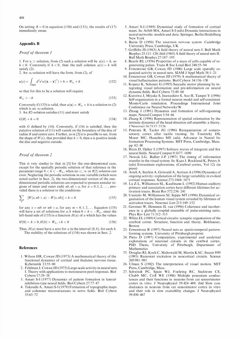
Proof of theorem 1

1. For a solution, from (2) such a solution will be x , so ` 0. Conversely if ` 0, then the null solution x willsatisfy (2).2. An I-solution will have the form, from (2), of

x

x

d 2 xHjx À xHj2 I 132

so that for this to be a solution will require

I b À 133

Conversely if (133) is valid, then x I is a solution to (2)which is an I-solution.3. An 2-solution satis®es (11) and must satisfy

q 0 134

with q de®ned by (16). Conversely, if (16) is satis®ed, then theputative solution of (11) will vanish on the boundary of the disc of radius and centre zero. Further, as in [3] it is possible to see, fromthe shape of x, that provided that ` 0, then is positive insidethe disc and negative outside.

Proof of theorem 2

This is very similar to that in [3] for the one-dimensional case,except for the spatially periodic solution of that reference in theparameter range 0 ` ` À I, when no , I or 2 solution canexist. Neglecting the periodic solutions in one variable (which were

noted earlier in Sect. 2), the two-dimensional version of the one-dimensional periodic solutions are expected to possess annular re-gions of inner and outer radii nY n , for n 0Y 1Y 2Y F F F Y pro-vided there is a solution to the conditions

n

xY n À xY n 0 135

for any x m or m , for any m 0Y 1Y 2Y F F F Equation (135)will have a set of solutions for Y when 0 ` ` À I, since theleft-hand side of (135) is a function r of which has the values

r 0 b 0Y r IY ` 0 136

Thus, r must have a zero for in the interval 0Y , for each .The stability of the solutions of (134) was shown in Sect. 2.

References

1. Wilson HR, Cowan JD (1973) A mathematical theory of thefunctional dynamics of cortical and thalamic nervous tissue.Kybernetik 13:55±80

2. Feldman J, Cowan JD (1975) Large-scale activity in neural netsI. Theory with applications to motoneuron pool responses. BiolCybern 17:29±38

3. Amari S-I (1977) Dynamics of pattern formation in lateral-inhibition type neural ®elds. Biol Cybern 27:77±87

4. Takeuchi A, Amari S-I (1979) Formation of topographic mapsand columnar microstructures in nerve ®elds. Biol Cybern

35:63±72

5. Amari S-I (1989) Dynamical study of formation of corticalmaps. In: Arbib MA, Amari S-I (eds) Dynamic interactions inneural networks: models and data. Springer, Berlin HeidelbergNew York

6. Burns D (1950) The uncertain nervous system. CambridgeUniversity Press, Cambridge, UK

7. Griths JS (1963) A ®eld theory of neural nets I. Bull MathBiophys 25:111±120; ibid (1965) A ®eld theory of neural nets II.

Bull Math Biophys 27:187±1958. Beurle RL (1956) Properties of a mass of cells capable of re-generating pulses. Trans R Soc Lond Biol 240:55±94

9. Ermentrout GB, Cowan JD (1980) Large scale spatially or-ganized activity in neural nets. SIAM J Appl Math 38:1±21

10. Ermentrout GB, Cowan JD (1979) A mathematical theory of visual hallucination patterns. Biol Cybern 34:136±150

11. Kopecz K, Schoner G (1995) Saccadic motor planning by in-tegrating visual information and pre-information on neuraldynamic ®elds. Biol Cybern 73:49±60

12. Kuroiwa J, Miyake S, Inawashiro S, Aso H, Tampri Y (1996)Self-organization in a formal neuron model and self-consistentMonte-Carlo simulation. Proceedings International JointConference on Neural Networks'96

13. Zhang J (1991) Dynamics and formation of self-organisingmaps. Neural Comput 3:54±66

14. Zhang K (1996) Representation of spatial orientation by theintrinsic dynamics of the head-direction cell ensemble: a theory.J Neurosci 16:2112±2126

15. Petersen R, Taylor JG (1996) Reorganisation of somato-sensory cortex after tactile training. In: Touretzky DS,Mozer MC, Hasselmo ME (eds). Advances in Neural In-formation Processing Systems. MIT Press, Cambridge, Mass.pp 82±88

16. Horn D, Opher I (1997) Solitary waves of integrate and ®reneural ®elds. Neural Comput 9:1677±1690

17. Nowak LG, Bullier J-P (1997) The timing of informationtransfer in the visual system. In: Kaas J, Rockland K, Peters A(eds) Extrastriate explorations. (Cerebral cortex, Vol 12) (inpress)

18. Arieli A, Sterkin A, Grinvald A, Aertsen A (1996) Dynamics of

ongoing activity: explanation of the large variability in evokedcortical responses. Science 273:1868±187119. Lu Z-L, Williamson SL, Kaufmann L (1992) Human auditory

primary and association cortex have dierent lifetimes for ac-tivation traces. Brain Res 572:236±241

20. Uusitalo M, Williamson SJ, Seppa MT (1996) Dynamical or-ganisation of the human visual system revealed by lifetimes of activation traces. Neurosci Lett 213:149±152

21. Gerstner W, Hemmen JL van (1996) Coherence and incoher-ence in a globally coupled ensemble of pulse-emitting units.Phys Rev Lett 71:312±315

22. White EL (1989) Cortical circuits: synaptic organisation of thecerebral cortex. Structure, function and theory. Birkhauser,Boston

23. Ermentrout B (1997) Neural nets as spatio-temporal pattern-forming systems. University of Pittsburgh preprint

24. Pinto D (1997) Computation, experimental and analyticalexplorations of neuronal circuits in the cerebral cortex.PhD Thesis, University of Pittsburgh, Department of Mathematics

25. Douglas RJ, Koch C, Mahowald M, Martin KAC, Suarez HH(1995) Recurrent excitation in neocortical circuits. Science269:981±985

26. Ulman S (1982) The interpretation of visual motion. MITPress, Cambridge, Mass.

27. Schwindt PC, Spain WJ, Foehring RC, Stafstrom CE,Chubb MC, Crill WE (1988) Multiple potassium conduc-tances and their functions in neurons from cat sensorimotorcortex in vitro. J Neurophysiol 59:424±449; ibid Slow con-ductances in neurons from cat sensorimotor cortex in vitroand their role in slow excitability changes. J Neurophysiol

59:450±467

408



28. Barbas H, Pandya DN (1992) Patterns of connections of theprefrontal cortex in the rhesus monkey associated with corticalarchitecture. In: Levin HS, Eisenberg HM, Benton AL (eds)Frontal function and dysfunction. Oxford University Press,Oxford

29. Mesulam MM (1981) Patterns of behavioural anatomy: asso-ciation areas, the limbic system and hemispheric specialisation.Ann Neurol 10:309±325

30. Taylor JG (1997) Invited talk. World Joint Conference onNeural Networks, Washington, DC

31. Petersen RS (1997) The neural ®eld theory approach to corticalself organisation. PhD Thesis, University of London, King'sCollege, Department of Mathematics

32. Swindale NV (1996) The development of topography in thevisual cortex: a review of models. Network: computation inneural systems 7:161±247

33. Miller KD, Keller JB, Stryker MP (1989) Ocular dominancecolumn development: analysis and simulation. Science245:605±615

409

J.G. Taylor- Neural `bubble' dynamics in two dimensions: foundations

Documents

Transcript of J.G. Taylor- Neural `bubble' dynamics in two dimensions: foundations