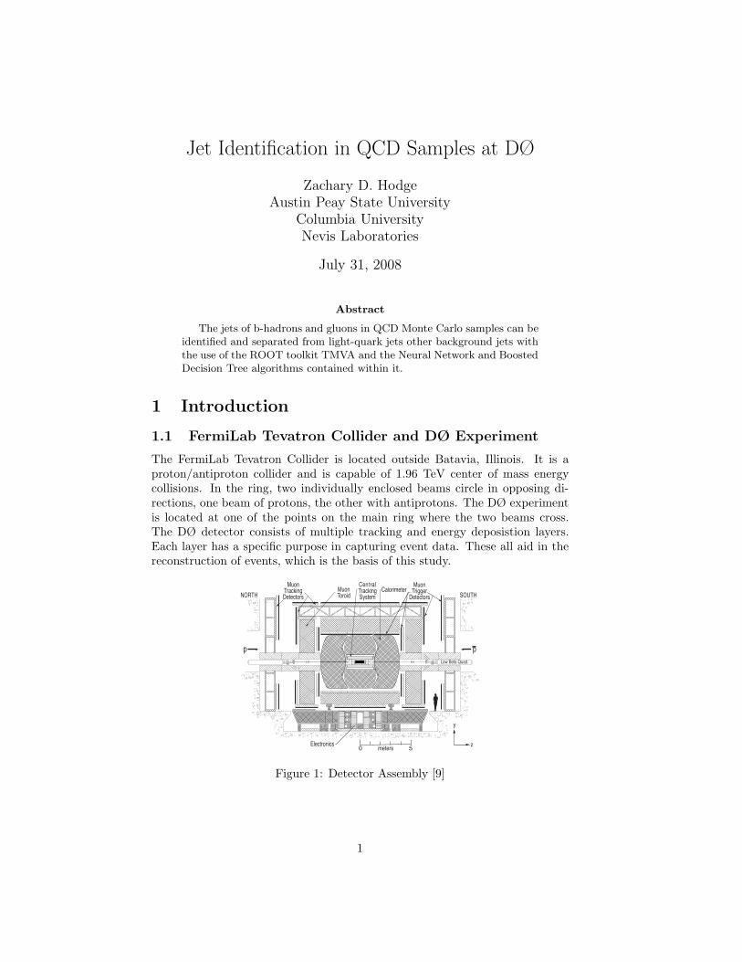
Jet Identification in QCD Samples at DØ

Zachary D. Hodge

Austin Peay State University

Columbia University

Nevis Laboratories

July 31, 2008

Abstract

The jets of b-hadrons and gluons in QCD Monte Carlo samples can be

identified and separated from light-quark jets other background jets with

the use of the ROOT toolkit TMVA and the Neural Network and Boosted

Decision Tree algorithms contained within it.

1 Introduction

1.1 FermiLab Tevatron Collider and DØ Experiment

The FermiLab Tevatron Collider is located outside Batavia, Illinois. It is aproton/antiproton collider and is capable of 1.96 TeV center of mass energycollisions. In the ring, two individually enclosed beams circle in opposing di-rections, one beam of protons, the other with antiprotons. The DØ experimentis located at one of the points on the main ring where the two beams cross.The DØ detector consists of multiple tracking and energy deposistion layers.Each layer has a specific purpose in capturing event data. These all aid in thereconstruction of events, which is the basis of this study.

Figure 1: Detector Assembly [9]

1

1.1.1 Silicon Detector and Fiber Tracker

The central tracking detectors provides the capability of measuring chargedparticles originating from the point where the initial interaction of the protonand antiproton collide (primary vertex). The silicon microstrip tracker (SMT)and central fiber trackers (CFT) surround the beam pipe, the inner most partof the detector. The SMT helps determine the position of charged particles nearthe location of the primary vertex and the CFT determines a charged particle’smomentum and charge. Directly outside of the fiber tracker is a solenoid capableof producing a 2T magnetic field. A charged particle’s path will bend while inthe presence of a magnetic field, this allows the trackers determine charge andmomentum.

Figure 2: Inner Tracking Chamber [9]

1.1.2 Liquid Argon Calorimeter

Outside of these trackers is the liquid Argon (LArg) and depleted Uraniumelectomagetic and hadroninic calorimeter. The calorimeter provides the abilityto measure the energy of electromagnetically and strongly interacting particles.The calorimeter is divided into 3 regions and each are fully enclosed to helpmaintain the liquid Argon at a constant 90K . The electromagnetic calorimeteruses sheets of depleted uranium as the absorber material, where as the hadroniccalorimeter uses copper. The absorber material is very dense and causes aparticle to radiate as it passes through it. This subsequently causes a shower ofparticles to be produced which ionize the liquid argon and allow for a signal tobe collected. This provides the ability to determine a particle’s energy as it iscompletely deposited in the detector.

1.1.3 Muon Tracking System

Surrounding all of these detectors is the muon tracking system. The muontracking system uses a magnetic field and drift chambers to track muons. A 2Ttorodial magnetic field is used to bend muon paths and determine momentum.Drift chambers provide the ability to track a muons position.

2

Figure 3: LArg E&M and Hadronic Calorimeter [9]

1.2 Bottom quarks, Hardronization, and Jets

At the FermiLab Tevatron Collider protons and antiprotons are accelerated inopposite directions and then crossed to produce collisions with center of massenergies of 1.96 Tev. During one of these collisions, many different particlesare produced. Many of these particles can be tracked and measured throughthe use of the detector described previously. Some processes cannot be measuredirectly, such as the top quark and Higgs boson production (Figure 5). Theseprocesses are very interesting, and can be evaluated through the existence ofbottom quarks in thier decays.

1.2.1 Bottom quarks

Bottom quarks are a third generation fermion and have a significantly highermass (4.2 GeV) than all the other quarks, excluding the top. The third genera-tion is named this because it was the last grouping to be discovered. Fermionsare particles with 1/2 integer spins (obey Pauli Exclusion Principle)and con-tained within this family are quarks and leptons. Bottom quarks carry a frac-tional electric charge of -1/3e. Bottom quarks are produced in many differentways. Some processes which can create bottom quarks are a top quark whichwill deacy into atleast two and possibly six bottom quarks. Also the decay ofthe theoretical Higgs boson is expected to decay in a similar way, producingbottom quarks.

1.2.2 Hadronization and Jets

Color charged particles (parton) do not exist freely, and will immediately forma bound state with another parton that is created from the vacuum. This is dueto color confinement, which is where a parton is stretched in its bound state,and finds a more energetically appealing situation if another parton is createdto bind to. This process is known as hadronization. Quarks will hadronize intoeither a meson or baryon. Mesons are a two quark configurations and Baryonsare three quark configurations. B-hadrons have a relatively longer lifetime thanother light-quark hadrons, of approximately 10−12 s, and therefore travel a fewmillimeters before decaying. The created hadron will then procede to decay andproduce even more particles, forming a collimated spray of paticles known as

3

Figure 4: Standard Model of Elementary Particles [11]

a jet.This jet can be detected in the elecromagnetic and hadronic calorimeter.The data collected on the jet can be reconstructed to infer the existence of theparton and further study its characteristics.

Figure 5: gg → Htt̄ Feynman Diagram [10]

2 Variables, selection and KS Test

2.1 Algorithms and Variables

There a currently four separate b-tagging algorithms used at DØ. Three ofwhich rely on charged particle tracks to differentiate between b-jets and light-jets, while the fourth uses the presence of a muon. Particles hits in the detectorthat leave a straight line are known at tracks. The DØ Neural Network (NN)

4

uses a list of predefined variables from the tagging algorithms to determinewhether a jet presents the charateristics of a b-jet or that of other light-quarkjets. The neural network connects many different, seemingly uncorrelated datainto a single variable.

2.1.1 Jet Tagging Algorithms

The Counting Signed Impact Parameters (CSIP) algorithm counts thetracks contained within a jet that have an large impact parameter significanceto the primary vertex. The Jet Lifetime Probability Tagger (JLIP) uses theimpact parameters from all tracks within a jet and combines it to one variable,the Jet Lifetime Probability (JLIP Prob). The Secondary Vertex Tagging

(SVT) uses the tracks from a jet that are displaced from the primary vertex,then reconstruct a displaced vertex based on those tracks. The Soft Lepton

Tagging (SLT) uses the presence of muon in the jet to tag it.

2.2 Selection of Variables based on a KS Test

Each of the algorithms produce sets of variables that can help in further dis-crimination of b-jets from light jets. The Kolmogorov-Smirnov goodness of fittest is used to determine which of the variables provide the greatest separationpower between b-jets and light jets.

2.2.1 Kolmogorov-Smirnov Test

A Kolmogorov-Smirnov (KS) Test is a goodness of fit test, used to determinethe difference between two one-dimensional distributions.

Dn,n′ = sup |Fn(x) − Fn′(x)| (1)

The KS test compares the locations of two empirical cumulative distributionfunctions to determine the greatest distance between the two. Variables witha higher KS value have distributions that differ significantly and thus providegreater separation power between the two distributions. The KS test is calcu-lated over all variables to determine which have the greatest separation power.

2.2.2 KS Test results and Variable Selection

The final variables are selected by choosing those with the greastest separationbetween b-jet and light jet samples. The variables are ranked from greatestseparation to least, and the top 24 variables were chosen to be used. See Table1 for the list of selected variables and corresponding KS values. The table is alist of variables created by its corresponding jet tagging algorithms. For examplesvt dlsig is the decay length significance (dlsig) as calcutated by the SecondaryVertex Tagging (svt) algorithm.

3 MLP and BDT

3.1 ROOT and TMVA

This entire study was done using ROOT and the TMVA program containedwithin it. The ROOT framework provides the platform to do data set on the

5

Variable KS Valuesvt dlsig 0.5570nn all out 0.5376svt dl 0.5178svt dlsig z 0.5048svt dl 3d 0.4717svt dlsig 3d 0.4601svt dl z 0.3927jlip prob 0.3076nn all csip comb 0.2912svt lifetime 0.2501svt svtrkpt 0.2127svt svpt 0.2126svt mass 0.1999svt ptcormass 0.1997svt ptrel 0.1985svt ntracks 0.1985svt ntracks sv 0.1980svt trkpt 0.1902svt ntracks pv 0.1828svt chisq 0.1627jlip ntracks 0.1365svt chisqndof 0.1318jet numtracks 0.1127jet ntracks cpf0 0.1034

Table 1: Komogorov-Smirnov Test Results

order of gigabytes or larger. The ROOT integrated TMVA package allows forhigher level data analysis through the use of the assorted classifier algorithms.

3.1.1 ROOT

The ROOT system is based on an object oreiented framework that providesthe capability of processing and analyzing significatly large amounts of data.ROOT has a large library of predefined functions that aid in histogrammingand assorted data analysis. The main feature of ROOT is the tree system, thatallows the access of specific parts of the data, rather than the whole.

3.1.2 TMVA

The Toolkit for MultiVariate Analysis (TMVA) is a ROOT integrated data pro-cessing and analysis package. TMVA uses mulitiple variable data sets to train,test and do performance evaluation on different classifier algorithms. Classifiersare prewritten data analysis algorithms that is contained in the TMVA package.

3.2 Multi-layer Perceptron Neural Network

Within the TMVA package is the artificial neural network (ANN) event classi-fier known as the multi-layer perceptron (MLP). Data is fed to the MLP at the

6

input layer, then sent to the first hidden layer where the data is analyzed anddetermined whether it presents background or signal like qualities. The MLPcontains hidden layers that each do analysis on the data to further separatesignal from background. Each hidden layer calculates some linear combinationof the input variables, compares its results to known signal and backgroundevents, calculates the error, and then reweights and repeats the process. MLPsare known as a feedforward architecture, meaning it sends information learnedon one hidden layer to the next hidden layer. The output of the MLP ANNsrequire training to be effective at differentiating between a signal event and abackground event and are therefore trained on 3000 known signal and back-ground events.

3.3 Boosted Decision Tree

Boosted decision trees (BDT) are a form of binary decision tree that operate ona yes/no decision as to what the variable should be classified as. BDTs oper-ate over one variable at a time, performing individual decisions that culminatein either classifiying that variable as signal or background. Figure 5 shows aschematic of a decision tree. Once passing through each layer of the tree, thevariable will reach a terminal node (leaf) that classifies it as either signal orbackground as a result of the path it took to reach that leaf. Statistical fluctua-tion in a sample can lead to a misclassification on a variable. Misclassification iswhere a known signal event lands on a background terminal node or vice versa.To account for these misclassifications, the decision tree undergoes a processknown as boosting. The act of boosting is training a variable several timesusing a boosted (reweighted) sample. Each time a variable is misclassified, it isrewieghted to make it signal like, then is repeated in the BDT. This helps todecrease statistical fluctuation in the response as a result of the training sample.

Figure 6: Decision Tree

7

3.4 Comparison of MLP and BDT

The background rejection versus signal effeciency curves of the MLP and BDTclassifiers were compared to determine which provided better feedback at sep-arating b-jets from light-quark jets. Both the BDT and decorrelated BDT(BDTD) showed a greater perfomance over the MLP of appoximately 3%. (SeeFigure 6) Because of the performance boost in the BDT classifier, it was chosento carry out the remainder of the study. Futher investigation was put into de-termining what the best setting were for the BDT. Figure 7 shows multiple testson the different BDT settings, with BDT5 exhibiting the greatest performancecurve(another 3% perfomance gain). The settings to achieve this (BDT5) areas follows:

• NTrees=1000

• BoostType=AdaBoost

• SeparationType=GiniIndex

• NCuts=20

• PruneMethod=ExpectedError

• PruneStrength=5

Signal efficiency0 0.1 0.2 0.3 0.4 0.5 0.6 0.7 0.8 0.9 1

Bac

kgro

un

d r

ejec

tio

n

0.2

0.3

0.4

0.5

0.6

0.7

0.8

0.9

1

Signal efficiency0 0.1 0.2 0.3 0.4 0.5 0.6 0.7 0.8 0.9 1

Bac

kgro

un

d r

ejec

tio

n

0.2

0.3

0.4

0.5

0.6

0.7

0.8

0.9

1

MVA Method:BDTBDTDMLP

Background rejection versus Signal efficiency

Figure 7: Background Rejection vs. Signal Effciency of MLP, BDT, and BDTD

4 Boosted Decision Tree with Variables

4.1 BDT on Z → bb Monte Carlo Sample

The BDT was trained and tested using Z → bb Monte Carlo samples to deter-mine the ability of the BDT to separate b-jets from light-quark jets. Predefined

8

signal eff0 0.1 0.2 0.3 0.4 0.5 0.6 0.7 0.8 0.9 1

bac

kgr

reje

ctio

n (

1-ef

f)

0.2

0.4

0.6

0.8

1

MVA_BDT

BDTBDT2BDT3BDT4BDT5BDTFULL

MVA_BDT

Figure 8: Background Rejection vs. Signal Effeciency on Multiple BDT Settings

Z → bb trees were input as signal events and Z → qq were input as backgroundevents.

4.1.1 Results of BDT with b-jets and light-quark jets

It is fairly obvious that the BDT was capable of separating b-jets from light-quark jets (See Figure 8). The background and signal distributions show aconsiderable difference. Background events are shifted toward a -1 value, whereas the signal events are shifted to a +1 value. There is a little crossing betweenthe two distribution around 0 but this is small compared to where the bulk islocated.

4.2 BDT on quark/gluon/other jets Monte Carlo Sample

The BDT was trained and tested using quark jets, gluon jets, and backgroundother jets Monte Carlo Samples to determine the ability of the BDT to separatequark jets from gluon jets and other jets in the event. An event sample waspreprocessed with cuts to artificially separate the quark jets, gluon jets andother jets from the MC sample.

4.2.1 Results of BDT with quark jets and other jets

The first BDT test was operated over all quark jets as signal and other jetsas the background.Other jets are are jets produce from some interaction thatis not directly related to a quark or gluon event. The BDT shows fairly goodcapability of separating the two jet types (See Figure 9). The Backgroundrejection vs signal efficiency curve shows a decrease efficiency, but this can be

9

BDT response-0.8 -0.6 -0.4 -0.2 0 0.2 0.4 0.6

No

rmal

ized

0

0.5

1

1.5

2

2.5

3SignalBackground

BDT response-0.8 -0.6 -0.4 -0.2 0 0.2 0.4 0.6

No

rmal

ized

0

0.5

1

1.5

2

2.5

3

U/O

-flo

w (

S,B

): (

0.0,

0.0

)% /

(0.0

, 0.0

)%

TMVA response for classifier: BDT

Figure 9: BDT Classifier Response: Signal = b-jets Background = light-quarkjets

attributed to the way cuts were applied in preprocessing to separate the jets.All jets were required to have atleast two tracks, which consequently makes theother jets have characteristics like that of quark jets. With this considered theBDT still shows good ability in separating the two.

4.2.2 Results of BDT with quark jets and gluon jets

The second test using the BDT classifier was on quark jets set as signal andgluon jets set as background. This test showed a significatly lower performancethan all previous tests. The BDT had difficulty separating quark and gluon jets.The output distributions are nearly overlapping (See Figure 12) and has a verylow efficiency curve (See Figure 13). These results are not unexpected though,as many of the variables for quark and gluon jets have similar distributions andvalues.

5 Conclusion

This study showed that through the use of TMVA and the Boosted DecisionTree (BDT) classifier algorithm, assorted high energy jets can be separated inMonte Carlo samples. The BDT classifier showed a ~3% efficiency gains overthe Multi-layer Perceptron (MLP) in separating b-jets. The BDT classifier alsoshowed ability in separating all quark jets from other background jets. TheBDT’s separation power was supressed in quark and gluon jets but this can beattributed to the similiar variable characteristics in the two jets. The BoostedDecision Tree has proven to be a capable classifier algorithm in jet separation.

10

Signal efficiency0 0.1 0.2 0.3 0.4 0.5 0.6 0.7 0.8 0.9 1

Bac

kgro

un

d r

ejec

tio

n

0.2

0.3

0.4

0.5

0.6

0.7

0.8

0.9

1

Signal efficiency0 0.1 0.2 0.3 0.4 0.5 0.6 0.7 0.8 0.9 1

Bac

kgro

un

d r

ejec

tio

n

0.2

0.3

0.4

0.5

0.6

0.7

0.8

0.9

1

MVA Method:BDT

Background rejection versus Signal efficiency

Figure 10: Background Rejection vs Signal Efficiency b-jets and light-quark jets

BDT response-0.8 -0.6 -0.4 -0.2 0 0.2 0.4 0.6 0.8

No

rmal

ized

0

1

2

3

4

5 SignalBackground

BDT response-0.8 -0.6 -0.4 -0.2 0 0.2 0.4 0.6 0.8

No

rmal

ized

0

1

2

3

4

5U

/O-f

low

(S

,B):

(0.

0, 0

.0)%

/ (0

.0, 0

.0)%

TMVA response for classifier: BDT

Figure 11: BDT Classifier Respones: Signal = quark jets Background = otherjets

11

Signal efficiency0 0.1 0.2 0.3 0.4 0.5 0.6 0.7 0.8 0.9 1

Bac

kgro

un

d r

ejec

tio

n

0.2

0.3

0.4

0.5

0.6

0.7

0.8

0.9

1

Signal efficiency0 0.1 0.2 0.3 0.4 0.5 0.6 0.7 0.8 0.9 1

Bac

kgro

un

d r

ejec

tio

n

0.2

0.3

0.4

0.5

0.6

0.7

0.8

0.9

1

MVA Method:BDT

Background rejection versus Signal efficiency

Figure 12: Background Rejection vs Signal Efficiency quark jets and other jets

BDT response-0.4 -0.3 -0.2 -0.1 0 0.1 0.2

No

rmal

ized

0

1

2

3

4

5

6 SignalBackground

BDT response-0.4 -0.3 -0.2 -0.1 0 0.1 0.2

No

rmal

ized

0

1

2

3

4

5

6U

/O-f

low

(S

,B):

(0.

0, 0

.0)%

/ (0

.0, 0

.0)%

TMVA response for classifier: BDT

Figure 13: BDT Classifier Response: Signal = quark jets Background = gluonjets

12

Signal efficiency0 0.1 0.2 0.3 0.4 0.5 0.6 0.7 0.8 0.9 1

Bac

kgro

un

d r

ejec

tio

n

0.2

0.3

0.4

0.5

0.6

0.7

0.8

0.9

1

Signal efficiency0 0.1 0.2 0.3 0.4 0.5 0.6 0.7 0.8 0.9 1

Bac

kgro

un

d r

ejec

tio

n

0.2

0.3

0.4

0.5

0.6

0.7

0.8

0.9

1

MVA Method:BDT

Background rejection versus Signal efficiency

Figure 14: Background Rejection vs Signal Effiency BDT quark jets and gluonjets

13

References

[1] Ay, C. Bernius, C., Hohlfeld, H., Kuhl, T., Meder-Marouelli, D., Tap-progge, S., Trefzger, T., Weber, G., Zeitnitz, C., “The DØ Experiment atthe Tevatron Accelerator,” 2004.

[2] Bachacou, H., Feligioni, L., “b-tagging at the Tevatron,” May 2007.

[3] Dutt, S., Gustavo, O.,“Taggability Studies in p20,” May 2008.

[4] Gadfort, T., “Evidence for Electroweak Top Quark Production in Proton-Antiproton Collisions at sqrt(s) = 1.96 TeV,” 2007.

[5] Hocker, A., Speckmayer, P., Stelzer, J., Tegenfeldt, F., Voss, H., Voss,K.,“TMVA Users Guide,” Toolkit for Multivariate Analysis with ROOT,June 2007.

[6] Roe, B., Yang, H., and Zho, J., “Boosted Decision Trees, A PowerfulEvent Classifier,”

[7] Scanlon, T., “A Neural Network b-tagging Tool,” August 2007.

[8] http://www-d0.fnal.gov/Run2Physics/displays/presentations

[9] http://www-d0.fnal.gov/Run2Physics/WWW/drawings/run2 nim

[10] http://www.physics.ndsu.nodak.edu/people/pilling/feynman.jpg

[11] http://en.wikipedia.org

14