
Jere R. Behrman, Yingmei Cheng, and Petra E. Todd*
25
EVALUATING PRESCHOOL PROGRAMS WHEN LENGTH OF EXPOSURE TO THE PROGRAM VARIES: A NONPARAMETRIC APPROACH Jere R. Behrman, Yingmei Cheng, and Petra E. Todd* Abstract—Nonexperimental data are used to evaluate impacts of a Boliv- ian preschool program on cognitive, psychosocial, and anthropometric outcomes. Impacts are shown to be highly dependent on age and exposure duration. To minimize the effect of distributional assumptions, program impacts are estimated as nonparametric functions of age and duration. A generalized matching estimator is developed and used to control for nonrandom selectivity into the program and into exposure durations. Comparisons with three groups—children in the feeder area not in the program, children in the program for 1 month, and children living in similar areas without the program—indicate that estimates are robust for significant positive effects of the program on cognitive and psychosocial outcomes with 7 months’ exposure, although the age patterns of effects differ slightly by comparison group. I. Introduction T here is growing recognition that human capital invest- ments made in early childhood are important determi- nants of school performance and lifetime productivity. 1 Previous studies suggest strong associations between (1) cognitive and psychosocial skills measured at young ages and (2) educational attainment, earnings, and employment outcomes. 2 In developing countries, low levels of investment in human capital are seen as a major barrier to growth as well as a source of poverty. Lower levels than in developed countries reflect the facts that children enroll later in ele- mentary school, repeat grades more frequently, and drop out of school at earlier ages. Recent research demonstrates that nutrition is an important factor in explaining delayed school enrollments and lower educational attainment levels. 3 To combat such problems, governments in several developing countries, often supported by international agencies, have introduced subsidized preschool programs with the twofold goals of improving child nutrition and providing environ- ments that are conducive to learning (Myers, 1995). In this paper, we evaluate the effectiveness of one such program, an early childhood development program in Bolivia called PIDI (Proyecto Integral de Desarrollo Infantil). There has been little research on preschool interventions in developing-country settings. However, a large literature evaluates the effects of preschool programs in the United States that are targeted at children from impoverished fam- ilies. 4 The Perry Preschool Program is perhaps the best known of the U.S. programs in the evaluation literature. An experimental evaluation of this program found that children who participated in it scored higher on cognitive tests, although the gains tended to disappear within a few years. Long-lasting effects were found on other outcome mea- sures, such as educational attainment, earnings, welfare participation rates, out-of-wedlock birth rates, and crime rates. 5 Evaluations of two other early intervention programs, the Milwaukee and Abecedarian projects, document long- lasting effects on test scores (Ramey, Campbell, and Blair, 1998). The positive impacts consistently found for interven- tions aimed at very young children are in sharp contrast to the relatively weak impacts often found in evaluations of U.S. job training programs targeted at adolescent youth or adults (for example, Bloom et al., 1993). Although the promising results from U.S. preschool pro- gram evaluations might lead to high expectations about similar programs in other settings, the results from U.S. experience may not be generalizable to developing coun- tries. Both the preschool programs and the families and children they aim to help differ in some possibly important respects. For example, program expenditure per child in developing countries is usually lower, although as a fraction of the family’s income it may be higher. Lower levels of expenditure do not necessarily imply low impacts, however, because diminishing marginal returns to investment could lead to higher impact per unit of investment. Another difference in developing countries is that preschool provid- ers are often less well trained. Lastly, in terms of the target population, children frequently suffer from protein and energy malnutrition and micronutrient deficiencies, which is why preschool programs in developing countries tend to put greater emphasis on nutrition. Such differences in program Received for publication November 19, 2002. Revision accepted for publication September 4, 2003. * University of Pennsylvania; Florida State University; and University of Pennsylvania and NBER, respectively. This research is sponsored by the World Bank Research Foundation Project on “Evaluation of the Impact of Investments in Early Childhood Development on Nutrition and Cognitive Development” (P. I. Harold Alderman). This paper was presented at the 2000 World Congress meet- ings of the Econometric Society. We thank Harold Alderman, Alfonso Flores-Lagunes, Judith McGuire, John Newman, Steven Stern, Edward Vytlacil, and participants at seminars at the University of Minnesota, Lehigh University, University of Delaware, University of Virginia, Uni- versity of Pennsylvania, Hebrew University, Ohio State University, and the NBER for helpful comments. We are also grateful to Elizabeth Pen ˜aranda of the PAN staff in La Paz, Bolivia, for help in understanding the details of the program being evaluated and of the data. We thank an anonymous referee and the editor Robert Moffit for many useful sugges- tions. Todd thanks the NSF for support under SBR-9730688. 1 This view is expressed, for example, in the United States Congress’s 1994 stated goal to send every child to school “ready to learn.” Goals 2000: Education America Act. 2 See for example Currie and Thomas (1999), Neal and Johnson (1996). 3 See Glewwe and Jacoby (1995), Alderman et al. (2001), Glewwe, Jacoby, and King (2001), and Martorell (1999) for evidence for Ghana, Pakistan, the Philippines, and Guatemala. 4 See Barnett (1992) for a survey of the findings from evaluations of many different U.S. programs. 5 The Perry Preschool Program spent significantly more per pupil than is typically spent on preschool interventions ($7252/year, over a third more than the Head Start program, for example). Most of this expenditure went to teacher pay; the teachers tended to be highly trained professionals (Sweinhart & Weikart, 1998). The Review of Economics and Statistics, February 2004, 86(1): 108–132 © 2004 by the President and Fellows of Harvard College and the Massachusetts Institute of Technology
Transcript of Jere R. Behrman, Yingmei Cheng, and Petra E. Todd*
EVALUATING PRESCHOOL PROGRAMS WHEN LENGTH OF EXPOSURETO THE PROGRAM VARIES: A NONPARAMETRIC APPROACH
Jere R. Behrman, Yingmei Cheng, and Petra E. Todd*
Abstract—Nonexperimental data are used to evaluate impacts of a Boliv-ian preschool program on cognitive, psychosocial, and anthropometricoutcomes. Impacts are shown to be highly dependent on age and exposureduration. To minimize the effect of distributional assumptions, programimpacts are estimated as nonparametric functions of age and duration. Ageneralized matching estimator is developed and used to control fornonrandom selectivity into the program and into exposure durations.Comparisons with three groups—children in the feeder area not in theprogram, children in the program for�1 month, and children living insimilar areas without the program—indicate that estimates are robust forsignificant positive effects of the program on cognitive and psychosocialoutcomes with�7 months’ exposure, although the age patterns of effectsdiffer slightly by comparison group.
I. Introduction
There is growing recognition that human capital invest-ments made in early childhood are important determi-
nants of school performance and lifetime productivity.1
Previous studies suggest strong associations between (1)cognitive and psychosocial skills measured at young agesand (2) educational attainment, earnings, and employmentoutcomes.2
In developing countries, low levels of investment inhuman capital are seen as a major barrier to growth as wellas a source of poverty. Lower levels than in developedcountries reflect the facts that children enroll later in ele-mentary school, repeat grades more frequently, and drop outof school at earlier ages. Recent research demonstrates thatnutrition is an important factor in explaining delayed schoolenrollments and lower educational attainment levels.3 Tocombat such problems, governments in several developingcountries, often supported by international agencies, haveintroduced subsidized preschool programs with the twofold
goals of improving child nutrition and providing environ-ments that are conducive to learning (Myers, 1995). In thispaper, we evaluate the effectiveness of one such program,an early childhood development program in Bolivia calledPIDI (Proyecto Integral de Desarrollo Infantil).
There has been little research on preschool interventionsin developing-country settings. However, a large literatureevaluates the effects of preschool programs in the UnitedStates that are targeted at children from impoverished fam-ilies.4 The Perry Preschool Program is perhaps the bestknown of the U.S. programs in the evaluation literature. Anexperimental evaluation of this program found that childrenwho participated in it scored higher on cognitive tests,although the gains tended to disappear within a few years.Long-lasting effects were found on other outcome mea-sures, such as educational attainment, earnings, welfareparticipation rates, out-of-wedlock birth rates, and crimerates.5 Evaluations of two other early intervention programs,the Milwaukee and Abecedarian projects, document long-lasting effects on test scores (Ramey, Campbell, and Blair,1998). The positive impacts consistently found for interven-tions aimed at very young children are in sharp contrast tothe relatively weak impacts often found in evaluations ofU.S. job training programs targeted at adolescent youth oradults (for example, Bloom et al., 1993).
Although the promising results from U.S. preschool pro-gram evaluations might lead to high expectations aboutsimilar programs in other settings, the results from U.S.experience may not be generalizable to developing coun-tries. Both the preschool programs and the families andchildren they aim to help differ in some possibly importantrespects. For example, program expenditure per child indeveloping countries is usually lower, although as a fractionof the family’s income it may be higher. Lower levels ofexpenditure do not necessarily imply low impacts, however,because diminishing marginal returns to investment couldlead to higher impact per unit of investment. Anotherdifference in developing countries is that preschool provid-ers are often less well trained. Lastly, in terms of the targetpopulation, children frequently suffer from protein andenergy malnutrition and micronutrient deficiencies, which iswhy preschool programs in developing countries tend to putgreater emphasis on nutrition. Such differences in program
Received for publication November 19, 2002. Revision accepted forpublication September 4, 2003.
* University of Pennsylvania; Florida State University; and Universityof Pennsylvania and NBER, respectively.
This research is sponsored by the World Bank Research FoundationProject on “Evaluation of the Impact of Investments in Early ChildhoodDevelopment on Nutrition and Cognitive Development” (P. I. HaroldAlderman). This paper was presented at the 2000 World Congress meet-ings of the Econometric Society. We thank Harold Alderman, AlfonsoFlores-Lagunes, Judith McGuire, John Newman, Steven Stern, EdwardVytlacil, and participants at seminars at the University of Minnesota,Lehigh University, University of Delaware, University of Virginia, Uni-versity of Pennsylvania, Hebrew University, Ohio State University, andthe NBER for helpful comments. We are also grateful to ElizabethPenaranda of the PAN staff in La Paz, Bolivia, for help in understandingthe details of the program being evaluated and of the data. We thank ananonymous referee and the editor Robert Moffit for many useful sugges-tions. Todd thanks the NSF for support under SBR-9730688.
1 This view is expressed, for example, in the United States Congress’s1994 stated goal to send every child to school “ready to learn.”Goals2000: Education America Act.
2 See for example Currie and Thomas (1999), Neal and Johnson (1996).3 See Glewwe and Jacoby (1995), Alderman et al. (2001), Glewwe,
Jacoby, and King (2001), and Martorell (1999) for evidence for Ghana,Pakistan, the Philippines, and Guatemala.
4 See Barnett (1992) for a survey of the findings from evaluations ofmany different U.S. programs.
5 The Perry Preschool Program spent significantly more per pupil than istypically spent on preschool interventions ($7252/year, over a third morethan the Head Start program, for example). Most of this expenditure wentto teacher pay; the teachers tended to be highly trained professionals(Sweinhart & Weikart, 1998).
The Review of Economics and Statistics, February 2004, 86(1): 108–132© 2004 by the President and Fellows of Harvard College and the Massachusetts Institute of Technology
characteristics and the contexts in which they operate couldaffect the extent and type of benefit from the intervention.
The PIDI program analyzed in this paper provides day-care, nutritional, and educational services to children betweenthe ages of 6 months and 72 months who live in poor,predominantly urban areas. The goals are to improve healthand early cognitive/social development by providing childrenwith better nutrition, adequate supervision, and stimulatingenvironments. It is hoped that the program will also ease thetransition to elementary school, improve progression throughelementary grades, and raise school performance, all of whichare expected to increase postschool productivity.
Through PIDI, children attend full-time child care centerslocated in the homes of women living in low-income areastargeted by the program. These women are given training inchild care and loans and grants (up to $500) to upgradefacilities in their homes. Each PIDI center has up to 15children and approximately one staff member per five chil-dren, with additional staff provided when there is a largerproportion of infants. The program provides food to supply70% of the children’s nutritional needs as well as health andnutrition monitoring and educational activity programs. Theprogram cost has been estimated by Ruiz (1996) to beapproximately $43 per beneficiary per month, which issubstantial in a country where per capita annual GDP is$800 in exchange-rate-converted pesos, or $2540 in pur-chasing power parity terms. Approximately 40% of theexpenditure goes to the nutritional component of the pro-gram (World Bank, 1997).
This paper uses a large nonexperimental data set to assessthe impact of the PIDI program on multiple child outcomemeasures related to health, cognitive development, andpsychosocial skill development. As measures of health, weconsider standard anthropometric measures: height for ageand weight for age. To measure cognitive and psychosocialdevelopment, we use children’s scores on a battery of testsof bulk motor skills, fine motor skills, language and auditoryskills, and psychosocial skills.
For our study of the PIDI program, the sample size isapproximately 10 times larger than the sizes typically ob-served in experimental evaluations, and the data set isrepresentative of the entire population of program recipi-ents. However, there is self-selection among eligible chil-dren into the program, which poses a threat to the validity ofthe results. Although the comparison group data sets that weuse were chosen by a sampling scheme designed to increasecomparability with the families in the program, we still findsome important differences between the treatment and com-parison group families. For example, families with childrenin the program tend to have lower parental education levelsand incomes, a difference that would likely bias the esti-mated program impacts downward if not taken into account.This source of bias is partly offset by the fact that programparticipants tend to be older than nonparticipants, whichincreases their average test scores and anthropometric out-
comes. Our analysis shows the importance of carefullytaking into account age and family background differencesin analyzing the effects of the program.
We use matching methods to control for potential biasdue to nonrandom selectivity into the program. One meth-odological contribution this paper makes to the previousliterature on matching is to allow for a continuous dose oftreatment (corresponding to the number of months spent inthe program), whereas most of the existing literature as-sumes that treatment is binary or belongs to a discrete set oftreatment types. Two of the matching estimators that we useare justified under the assumption that selection into theprogram is on observables, that is, that it can be taken intoaccount by conditioning on observed family and childcharacteristics. We also develop an alternative marginalmatching estimator that allows selection into the program tobe based on unobservables, but assumes that conditionalupon having selected into the program, selection into alter-native program durations is on observables. An advantage ofthe marginal estimator is that it only requires data on thetreatment group and is thus implementable when no com-parison group data are available.
The results show that the program significantly increasescognitive achievement and psychosocial test scores, espe-cially for children who participated in the program for atleast 7 months. The impact estimates are fairly robust to theuse of alternative comparison groups and estimators. Esti-mates obtained by the marginal matching estimator tend tobe larger, particularly at longer durations and for childrenaged 6–36 months, than those obtained using traditionaleconometric estimators that impose stronger functional-form assumptions. Cost-benefit analysis based on our esti-mates and on evidence from wage studies for developingcountries indicates that the PIDI program may have fairlyhigh rates of return.
In section II of the paper, we develop a model of enroll-ment in preschool that gives an economic interpretation forthe average treatment effects that we estimate. Section IIIdescribes how we generalize existing matching estimatorsto accommodate a varying treatment dose as well as impactheterogeneity with respect to children’s ages, and introducesthe marginal effect estimators. Section IV provides addi-tional information about the PIDI program and data sets,analyzes the determinants of program participation, andpresents the impact estimates obtained by matching and, forcomparison, by more standard regression methods. SectionV performs a cost-benefit analysis based on our preferredmarginal effect estimates and other explicit assumptionsregarding subsequent schooling and wage effects. SectionVI concludes.
II. A Model of the Preschool Participation Decisionand Treatment Effects
We develop a model of the mother’s decision to enroll herchild in preschool, which provides a way of interpreting the
EVALUATING PRESCHOOL PROGRAMS 109
treatment effects that will be estimated later in the paper andgives some insight into which conditioning variables shouldbe used in the matching procedure. Our framework assumesthat the mother maximizes a time-separable utility functionthat depends on her own consumption (Ct
m) and leisure (stl)
and on the quality of her child (qt). There is a child qualityproduction function that depends on the mother’s timeallocated to child production (st
c), on the child’s consump-tion of household monetary resources (Ct
c), on whether thechild is in preschool, and on stochastic elements. Time notspent in leisure or child quality production is assumed to bespent working at wage wt
m.To focus only on the most relevant aspects, we abstract
from certain considerations. We assume that the father’sonly role is to contribute to the asset income At of thefamily, which is consumed in full every time period, andthat there is only one child of age at for whom the motheris making decisions. D*p,t is an indicator that takes a value 1if the mother would choose to enroll the child in thepreschool program were the child eligible, et is an indicatorthat equals 1 if the child is eligible. Dp,t is an indicator forwhether the child is actually enrolled. We assume a fixedcost K to the mother of enrolling in the preschool programand transporting the child to the program site.
The mother’s problem can be expressed as a dynamicprogramming problem, where the choices at any point intime are whether to enroll the child in preschool, how muchtime to invest in the child, how much time to spend inleisure, and how much consumption to allocate to the child.The set of period t state variables, denoted by �t, consistsof the child’s age, previous-period child quality, mother’swage, father’s income, and program participation cost.6 Therandom shocks in the model (εt
t, εtl, εt
q) are shocks to thevalue of mother’s consumption and leisure and to the childquality production function. The mother solves
Vt��t� � max�Ct
m,stc,D*P,t,st
l�
U�C tm, qt, st
l; εtt, εt
l, εtt�
� �E�Vt�1��t�1�C tm, st
c, D*P,t, stl, �t��
subject to constraints
qt � q�stc, Ct
c, DP,t, at, qt�1� � εtq, (1)
Ctm � Ct
c � Dp,tK � �1 � stc � st
l�wtm � At, (2)
DP,t � etD*P,t. (3)
Equation (1) describes the production technology for childquality, where we are assuming that previous-period qualityis a sufficient statistic for prior inputs,7 that εt
q represents a
shock realized after input decisions, and that the productiv-ity of inputs may depend on the child’s age. For example,preschool could be highly productive for a toddler but notfor a six-month-old infant. Equation (2) is the budgetconstraint, and (3) describes the constraint that preschool isonly an option for eligible families. We assume that mothersdo not try to influence their children’s eligibility (for exam-ple, by changing their labor force participation or by makingtheir children appear undernourished).
The total effect on child quality from participating inpreschool from time period t to t (the treatment effect ofswitching from state DP,t 0 to DP,t 1 for t � {t, t})can be expressed in terms of the model. It includes the directeffect that participation has on quality in the current periodas well as indirect effects that could occur, for example, ifthe mother reduces the child’s consumption at home know-ing that he/she receives meals at school. Let s1,t
c , s1,tl , C1,t
c
denote the values that solve the dynamic programmingproblem when DP,t 1, and let s0,t
c , s0,tl , C0,t
c denote thecorresponding values when DP,t 0.
The total effect of preschool participation on current-period quality for a particular child of age at who starts offat quality level qt�1 q� is given by
�qt
�DP,t� q�s1,t
c , C1,tc , 1, at, q� � � q�s0,t
c , C0,tc , 0, at, q� �.
The total program effect is inclusive of any compensatingchanges in the mother’s allocation of time and consumptionto the child. In addition, a change in current-period qualitylevels potentially affects future quality levels. For example,if a child starts off period t � 1 at a high quality level, heor she may be better able to take advantage of consumptionand time investments. The effect of increasing quality due toprogram enrollment at time t on future quality levels (attime t � t) is given by
�qt
�qt�1
�qt�1
�qt�2· · ·
�qt�1
�qt
�qt
�Dp,t.
Thus, the cumulative effect of being enrolled in preschool inperiods t through t is
�t,T � �vt
t � �qv
�DP,v� �
wv�1
T �qw
�qw�1· · ·
�qv�1
�qv
�qv
�DP,v�, (4)
where the first term captures the current-period impact andthe second term the impact on future quality levels up untilsome end period T.8
In the data analyzed in sections IV and V, we do notobserve children over the entire time period of their
6 For simplicity, there is no uncertainty about the wage, father’s income,or participation cost.
7 We make this assumption for simplicity. The assumption that previous-period quality is a sufficient statistic could be relaxed to allow quality todepend on the history of inputs over the child’s lifetime.
8 In writing the treatment effect solely as a function of effects on currentand future quality, we are also assuming that there are no effects ofanticipation of the program on quality levels prior to the program entrydate.
THE REVIEW OF ECONOMICS AND STATISTICS110
participation in the program (up to T), so we can onlyestimate the cumulative effect of the preschool treatment upuntil the time of observation, to. We assume that the empir-ical test scores and anthropometric measures available in thedata set capture aspects of child quality.9 The mean treat-ment effect we estimate (conditional on age and duration oftime in the program) using the matching estimators de-scribed in section III is equal to E(�t,to�age a, to � t l, DP 1), where DP 1 denotes participating in theprogram. The treatment effect depends on the productionfunction for quality, on the utility function determiningother input levels, and on the distribution of asset and wageincome among families.10
Next, we consider the question of how to choose the setof conditioning variables used in matching. Let q0t be thequality level when the child does not participate in theprogram at time t, and q1t the quality level when the childdoes participate. The decision to enroll the child at any timeperiod (which is only relevant for eligible families) impliesthat at that date, the current utility plus the expected futureutility from participating is higher than from not partic-ipating:
U�C0,tm , q0,t, s0,t
l ; εtl, εt
t�
� �E�Vt�1��t�1�C0,tm , s0,t
c , s0,tl , D*P,t, �t��
� U�C1,tm , q1,t, s1,t
l ; εtl, εt
t�
� �E�Vt�1��t�1�C1,tm , s1,t
c , s1,tl , D*P,t, �t��.
Define the outcomes in the no-program state and in theprogram participation state as
Yt�a, 0� � qt�DP,t0 for all t�t and
Yt�a, l � � Yt�a, 0� � �t,t�l,
and suppose that there is available a set of conditioningvariables Zt. The cumulative matching estimator describedin the next section assumes that
E�Yt�a, 0��Zt, D*P,t � 1, t � t0 · · · t�
� E�Yt�a, 0��Zt, et � 1, D*P,t � 0, t � t0 · · · t�.
The estimator also requires that Pr(D*P,t 0�Zt, et 1) �0, so that there is a positive probability of observing bothprogram participants and nonparticipants with the same
characteristics Zt. This requirement implies that, conditionalon Zt, there must be other variables affecting programparticipation and that these variables not be correlated withchild outcomes in the no-treatment state. For example,suppose that distance to the program site is a determinant ofparticipation and that the placement of program sites can beconsidered random with respect to child outcomes in theno-treatment state conditional on Zt. If Zt contains all theelements of the state space except distance, then the aboveexogeneity condition can be satisfied.
For reasons described later in the paper, it is importantnot to match on variables that themselves are affected by theprogram, such as the mother’s labor supply in the model.This is because the matching estimator (described below insection III) integrates over f(Zt�D*P,t 1). To estimatecorrectly the mean no-treatment outcomes, we require thatthe density of the matching variables do not change withtreatment. For this reason, we match on the following: (a)variables observed prior to the enrollment decision (underthe assumption that the density of these variables does notchange due to anticipation of the program), (b) variablesthat we expect to be stable over the time period of obser-vation (such as the mother’s and father’s education, thefamily structure, and the characteristics of the household),and (c) variables that are deterministic with respect to time(such as the child’s age). We do not include variables thatdirectly relate to children’s physical, mental, and socialdevelopment.
III. Cumulative and Marginal Matching Estimators
As discussed in the previous section, we are interested inestimating the treatment effect �t,t0 [defined in equation(4)], which gives the total effect of the preschool programon child quality for a child that participates in the programfor a duration l t � t0. We next describe the estimatorswe use and the assumptions required to justify their appli-cation. We go beyond the previous literature on matching byallowing for a continuous dose of treatment (given by theduration of time spent in the program), by permitting im-pacts to depend in a flexible way on children’s ages, and bydeveloping a marginal matching estimator that can be im-plemented if data on program participants are the only dataavailable.
Let Y(a, l ) denote the outcome measure intended tocapture an aspect of child quality (test score or anthropo-metric measure) for a child of age a who participated in theprogram for length of time l.11 For nonparticipants, l 0.Also define DP 1 if l � 0, DP 0 otherwise. For a childof age a, the cumulative impact of participating in theprogram l time periods relative to not participating is givenby �(a, l, 0) Y(a, l ) � Y(a, 0). Also of interest is themarginal effect of participating in the program l1 time
9 Preschool investments could increase the amount learned in school andlead to higher quality in elementary school years, but these benefits willnot be captured by our estimation approach, due to the data limitationposed by not observing children at these later ages. In the cost-benefitanalysis of section V, we will briefly consider these other sources ofbenefits.
10 Knowing the treatment effect of the program does not allow recoveryof the parameters of the production technology. Only under the strongassumption that parents do not alter their time or resource allocationswhen their child participates in the program would the treatment effectcorrespond to a feature of the production technology (see related discus-sion in Todd & Wolpin, 2003).
11 We assume participation takes place in consecutive time periods, as itdoes in our data.
EVALUATING PRESCHOOL PROGRAMS 111
periods relative to l0 time periods: �(a, l1, l0) Y(a, l1) �Y(a, l0). Neither of these program impacts is directlyobservable, because every child in the program is observedfor a single duration at each age and no child is observedsimultaneously in and out of the program at the same age.Because of this missing data problem, we do not attempt toestimate the full distribution of treatment impacts. We focusinstead, firstly, on the problem of estimating average treat-ment impacts, and secondly, on the problem of estimatingmarginal treatment impacts—in both cases, conditional onage and duration of exposure to the program. The averageprogram impact for children of age a � A who participatedl1 time periods as opposed to l0 (where l0 could equal 0) isgiven by
�� �A, l1, l0� � a�A �Y�a, l1� � Y�a, l0�� fa�a�l � l1�da
a�A fa�a�l � l1�da,
where fa(a�l l1) is the conditional density of ages and Acan be a singleton set or a range of ages.
Integrating over the joint density of observed ages andprogram durations gives the overall impact of the programrelative to the counterfactual of participating for length oftime equal to l0:
�� �A, L, l0� � l�L a�A �Y�a, l � � Y�a, l0�� fa,l�a, l �da
l�L a�A fa,l�a, l �da,
where L {l : l � 0}. Thus �� ( A, L, 0) gives the averageimpact of participating in the program relative to not par-ticipating for the DP 1 group, commonly known as theaverage impact of treatment on the treated. A comparison ofa monetary valuation of this impact with average programcosts is informative on whether the program has a positivenet benefit (see section V).
A. Estimators
We now give the identifying conditions that justify themethod of matching as a way of imputing the missing datarequired to estimate the average treatment effects definedabove, which relate to the treatment impacts defined interms of the economic model of section II.12
Estimating Program Impacts When the Counterfactual isNo Treatment: The matching method estimates no-program outcomes for program participants by takingweighted averages over outcomes for observably similarpersons who did not participate in the program. The degreeof similarity between two persons is determined by thedistance, according to some metric, between a set of theircharacteristics that constitute the matching variables. By
matching on the characteristics of the treatment group, themethod effectively aligns the distribution of observables ofthe comparison group with that of the treated group.13
The identifying assumption that justifies the matchingestimator that we use to estimate �� ( A, l, 0) is that thereexist a set of conditioning variables x such that
E�Y�a, 0��a, li � l, x� � E�Y�a, 0��a, li � 0, x� (5)
and
0 � f�a, x�DP � 0�. (6)
As discussed in section II, the first condition implies thatafter conditioning on a set of observed characteristics {a,x}, no-treatment outcomes for children who have partici-pated for duration l will be on average the same as thoseobserved for children who have not participated (DP 0).The second condition ensures that for each child in theparticipant group there is positive probability of finding amatch from the nonparticipant group.14 Let SP {(a, x) :f(a, x�DP 1) � 0 and f(a, x�DP 0) � 0} denote theregion of the support of (a, x) that satisfies equation (6),called the region of overlapping support.15
Under the above conditions, �� ( A, L, 0) can be estimatedby
�� �A, L, 0� �1
n�
i��DP1���ai�A���li�L����ai,li��SP�
�E�Y�ai, li��xi, DPi � 1� � E�Y�ai, 0��xi, DPi � 0��,
(7)
where n is the cardinality of the set {DP 1} � {ai � A} �{li � L} � {(ai, li) � SP}, and E(Y(ai, li)�xi, DPi 1)and E(Y(a, 0)�xi, DPi 0) are consistent estimators of theconditional expectations.
We estimate the conditional expectations using localnonparametric regression methods. The estimator E(Y(ai,0)�xi, DP 0) can be written compactly as
�k��DP0�
n0
Yk�ak, 0�Wk��ak � ai�, �Xk � Xi��, (8)
where Wk(�ak � ai�, � xk � xi�) are weights that sum to 1and that depend on the Euclidean distance between (ai, xi)and (ak, xk). For standard kernel weighting functions,
12 Matching methods have been developed and applied to the evaluationof training programs by Heckman, Ichimura, and Todd (1997), Heckman,Ichimura, Smith, and Todd (1998), Dehejia and Wahba (1999), Smith andTodd (2001, 2004), and others.
13 In performing this alignment, it emulates a feature of a randomizedexperiment in which the characteristics of the treatment and comparisongroups are aligned by virtue of randomization.
14 See Rosenbaum and Rubin (1983). Under both conditions, treatmentis termed strictly ignorable. If there are some (a, X) values for which thesecond support condition fails, then treatment impacts cannot be estimatedby the method of matching for individuals with those characteristics.
15 See Heckman, Ichimura, and Todd (1997) for discussion of supportconditions required in matching.
THE REVIEW OF ECONOMICS AND STATISTICS112

observations that are close according to the distance metricreceive greater weight. The nonparametric estimators weuse are local linear regression estimators that have beendeveloped and studied in Cleveland (1979) and Fan (1992).The details of local linear regression estimators are de-scribed in appendix B.16
The analogous nonparametric estimator for E(Y(ai, li)�xi,DPi 1) in equation (7) is
E�Y�a, l �� � �k��DP1�
Yk�ak, lk�Wk��lk � li�,
�ak � ai�, � xk � xi��,(9)
where the weights now additionally depend on the distancebetween lk and li (allowing the impact of the program todepend on the duration of time in the program).17 Note thatin equation (7) averaging is performed in two stages, oncein obtaining the nonparametric estimates and again in aver-aging over the set {DP 1} � {ai � A} � {li � L} �{(ai, li) � SP}. Because of the second averaging, theaverage impact estimators over ranges of age and durationvalues converge at a faster rate than the pointwise (in a andl ) estimators. The asymptotic theory of Heckman, Ichimura,and Todd (1998) is general enough to accommodate theestimators. In the empirical work, however, we evaluate thevariation of the estimators using bootstrap methods ratherthan variance estimators based on asymptotic formulas.
Estimating Marginal Program Impacts: Instead of (orin addition to) the impact of the program against the bench-mark of no program, we may be interested in the marginaltreatment effect of increasing duration in the program froml0 to l1: �� (a, l1, l0) E(Y(a, l1)�DP 1, x) � E(Y(a,l0)�DP 1, x), where l1, l0 � 0. There are two differentways of estimating marginal effects. One is to first estimatecumulative effects at different duration levels and then takethe difference. The other way is to use only data on programparticipants, drawing comparisons between program partic-ipants who have taken part in the program for differentlengths of time.
1. Marginal impact estimator based on difference incumulative effects. An estimator of the marginal effectfrom participating in the program for l1 time periodsas opposed to l0 time periods (l1 � l0) can beobtained as the difference between the two cumulativeprogram effects: �� (a, l1, l0) �(a, l1, 0) � �(a, l0,0). Estimating marginal effects in this way assumes
that the group of children observed participating in theprogram l0 periods provide an appropriate comparisongroup for the children observed participating l1 peri-ods—an assumption that may not be justified if chil-dren are systematically entering or dropping out fromthe program at different ages. Partly for this reason,we prefer the approach described next, which is theone we take in our empirical work.
2. Marginal impact estimator that only uses data onprogram participants. An alternative estimation strat-egy only uses data on program participants and com-pares outcomes for children of similar ages withdifferent durations. An advantage of this approachover the previous one is that it does not requireassumptions on the process governing selection intothe program and allows for the possibility that selec-tion into the program is based on unobserved charac-teristics. However, here we are faced with a differentpotential source of nonrandom selection—the processgoverning selection into alternative program dura-tions. For example, four-year-olds who have takenpart in the program for three years may be systemat-ically different from four-year-olds who just recentlyentered the program. Again, matching methods can beused to solve the selection problem relating to thechoice of program duration—under the assumptionthat children who have taken part in the program fordifferent lengths of time can be made comparable byconditioning on observed child and parental charac-teristics.
In our empirical application to the analysis of the PIDIprogram, a major determinant of duration in the program isthe time at which the program first became available tochildren, which differs across children depending on thechild’s place of residence and child’s age at the time thelocal PIDI site began its operation. Two-thirds of the chil-dren in the PIDI evaluation sample began participating inthe program as soon as it became available; on average, thedelay between the time the local PIDI site opens and thetime children begin participating is 3.2 months. The varia-tion in duration of time spent in the program that arises fromvariation in when the program became available to childrenis therefore arguably exogenous with respect to programoutcomes, conditional on observed child and parent charac-teristics.
Formally, the identifying assumption the marginal esti-mator invokes is that there exists a set of conditioningvariables x such that
E�Y�a, l0��l � l1, x, a� � E�Y�a, l0��l � l0, x, a�
and 0 � f(a, x�l l0). Under these assumptions, anestimator for �� (a, l1, l0) is given by
16 The numbers of observations used in constructing the averages aredetermined by the choice of bandwidth or smoothing parameter. We useleast squares cross-validation to choose these parameters as described insection IV.
17 An alternative approach would be to construct the weighted averagesin equation (8) over the set of observations k � {DP 1} � {l li}.Instead, we do local averaging over durations l because there may not bemany observations at any individual duration value.
EVALUATING PRESCHOOL PROGRAMS 113
�� �a, l1, l0� �1
n�
i��lil1�
�E�Y�a, l1��xi� � E�Y�a, l0��xi��.
The conditional expectations are estimated by the samelocal regression method as described in relation to equation(9).
�� �a, l1, l0� gives the effect of increasing the duration inthe program from l1 time periods to l0 time periods for theset of children who participated for length of time l1.Obtaining the effect of increasing the duration from l0 to l1
for the set of children who participated l0 time periodswould require summing over i � {li l0}.
Reducing the Dimension of the Conditioning Problem:The above estimation strategy is difficult to implement for alarge set of conditioning variables x. To reduce the dimen-sionality of the conditioning problem, we can use theinsights of Rosenbaum and Rubin (1983), who observedthat for random variables y and x and a discrete randomvariable D denoting assignment to a binary treatment,
E�D�y, P�D � 1�x�� � E�E�D�y, x��y, Pr�D � 1�x��,
so that E(D�y, x) E(D�x) implies E(D�Y, Pr(D 1�x)) E(D�Pr(D 1�x)). This shows that when no-treatment outcomes are independent of program participa-tion conditional on x, they are also independent of partici-pation conditional on P( x) Pr(D 1�x). Matching onthe probability of participation instead of on X directlyprovides a way of reducing the dimensionality of the con-ditioning problem when P( x) can be estimated parametri-cally or semiparametrically at a rate faster than the nonpara-metric rate.
In our context, by imposing strong conditional indepen-dence assumptions, we could apply the above reasoning toY(a, 0). However, for the purpose of estimating averageeffects of treatment, the assumption of conditional indepen-dence of outcomes and participation status is stronger thannecessary (see Heckman, Ichimura, & Todd, 1997). Instead,we assume directly that equation (5) holds when we replacex by P( x) Pr(DP 1�a, x). The conditional expecta-tions can then be estimated by three- and two-dimensionalnonparametric regressions:
E�Y�a, l ��P� x�, DP � 1� � �k��DP1�
Yk�ak, lk�
� Wk��lk � l�, �ak � a�, �P� xk� � P� x���,(10)
E�Y�a, 0��P� x�, DP � 0� � �k��DP0�
Yk�ak, 0�
� Wk���ak � a�, �P� xk� � P� x���.
In our empirical work, we estimate the conditional proba-bilities P( x) by logistic regression.18
Modifications Required to Accommodate Choice-basedSampled Data: In evaluation settings, data are oftenchoice-based sampled, meaning that program participantsare oversampled relative to their frequency in a randompopulation and weights are required to consistently estimatethe probabilities of program participation. However, therequired weights are often unknown. Heckman and Todd(1995) show that with a slight modification, matching meth-ods can still be applied to choice-based sampled data withunknown weights. They show that the odds ratio P( x)/[1 �P( x)] that is estimated using the wrong weights (ignoringthe fact that the data are choice-based sampled) is a scalarmultiple of the true odds ratio, which is a monotonictransformation of the propensity scores. Therefore, match-ing can proceed on the (misweighted) estimate of the oddsratio (or on the log odds ratio). In our empirical work, thedata are choice-based sampled and the sampling weights areunknown, so we match on the odds ratio.
Comparison with Regression-based Methods: In manyevaluations, some matching is carried out implicitly prior toapplying regression methods in selecting the comparisongroup to have certain features in common with the treatmentgroup. Individuals may be required to meet age, race,geographic location, income, or other criteria for inclusionin the sample. Matching methods aim to increase the com-parability between the treatment and comparison groupsamples by aligning the distribution of observed covariatesof comparison group members with that of the treatmentgroup. To see how realignment occurs, write the meanno-treatment outcome for program participants E(Y(a,0)�DP 1) Ex�DP1{EY(Y(a, 0)�DP 1, x)} as
�x�X
EY�Y�a, 0��DP � 1, x� f � x�DP � 1� dx
� �x�X
EY�Y�a, 0��DP � 0, x� f� x�DP � 1� dx
��x�X
EY�Y�a, 0��DP � 0, x� f�x�DP � 0�� f�x�DP � 1�
f�x�DP � 0��dx,
where the second equality follows under the assumptionsthat would justify the application of matching. The last line
18 Heckman, Ichimura, and Todd (1998) and Hahn (1998) considerwhether it is better in terms of efficiency to match on P(X) or on Xdirectly. For the treatment on the treated parameter, Heckman, Ichimura,and Todd (1998) show that neither is necessarily more efficient than theother. If the treatment effect is constant, then it is more efficient tocondition on the propensity score; but in the general case the answerdepends on the mean of the conditional variance relative to the varianceof the conditional mean.
THE REVIEW OF ECONOMICS AND STATISTICS114
shows that matching can be seen as a reweighting method,where comparison group observations are reweighted byf�x�D � 1�
f�x�D � 0�. The reweighting accomplished through match-
ing (or through a weighted regression) balances observedcharacteristics of the treatment and comparison groups.Such a balancing would also occur in a randomized exper-iment. Traditional regression-based estimators do not at-tempt to emulate the balancing feature of randomized ex-periments, but instead control for observable differencesbetween groups by assuming the conditional mean functionis correctly specified by the regression equation.19
Selection on Unobservables: The estimators for cumu-lative program effects described above assume that out-comes are mean-independent of program participation con-ditional on a set of observables. If the program participationequation can be described by the index model DP 1(�(Z) � V � 0), then the matching estimator assumesthat E(Y(a, 0)�x, V � �(Z)) E(Y(a, 0)�x). Thisassumption is not likely to be satisfied if unobservables thatare related to program outcomes are important determinantsof program selection. One option in this case is to use adifference-in-difference (DID) matching strategy that al-lows for time-invariant unobservable differences in theoutcomes between participants and nonparticipants (seeHeckman, Ichimura, and Todd, 1997). However, our data donot allow application of this estimator, because programparticipants are only observed after they already entered theprogram. As we show below, lack of preprogram (baseline)data is a limitation in the data for our study and makes itdifficult to estimate reliably the cumulative effects of theprogram. However, we can estimate the marginal impact ofshort versus long durations using the estimators, describedearlier in this subsection under “Estimating Marginal Pro-gram Impacts,” that allow selection into the program to bebased on unobservables.
IV. Empirical Results
A. The Data
The PIDI evaluation data sets consist of repeated cross-section data collected in two rounds on three differentsubsamples: (i) a participating subsample (P) of childrenselected randomly from children in the PIDI program, (ii) anonparticipant subsample (B) selected from a stratifiedrandom sample of households with at least one child in theage range served by PIDI living within a 3-block radius of
a PIDI site but without any children attending PIDI, and (iii)a comparison group subsample ( A) selected from a strati-fied random sample of households with children in the agerange served by PIDI living in poor urban communitiescomparable to those in which PIDI had been established, butin which PIDI programs had not yet been established at thetime of the survey.20 As noted above in section IIIA under“Reducing the Dimension of the Conditioning Problem,”the data are choice-based sampled with unknown populationweights. For this reason, we do not know the participationrate among all eligibles. Fortunately, this information is notneeded for our estimation strategy, but it would be requiredto implement some other common evaluation approaches.21
We estimate program impacts using both the comparisongroup samples A and B. Sample B has an advantage over Ain being drawn from the same area as the participant sampleP, which controls for unobserved local community effectsthat may affect children’s outcomes. However, sample Bfamilies elected not to participate in the program, so theoutcomes observed for B children may not be directlycomparable with those for P children. Sample A combinesdata on families that would have participated in the programhad the program been available as well as data on familiesthat would not have participated. Finally, to estimate mar-ginal program impacts, we compare children in the partic-ipating sample P who had been in PIDI for two or moremonths with children in P who had been in PIDI for onemonth or less.
All the children in sample P meet the eligibility criteriathat are summarized below in section IVB, but children inthe comparison samples A and B do not necessarily meet thecriteria. In our application of the matching estimators, weonly use subsamples of children from the samples A and Bwho satisfy the eligibility criteria.22 As described below,there was a change in the eligibility criteria over time. Weuse the later criteria rather than the earlier ones, because theearlier ones included subjective aspects, the application ofwhich we cannot duplicate with much confidence. The firstand most important (at least in the lexicographical orderingsense) of the original criteria is a child characteristic—beingmalnourished—that the program is attempting to affectdirectly. Because we do not have baseline data on children
19 Another difference between matching and regression estimators ishow they deal with the problem of nonoverlapping support. The matchingestimator is only defined over the support of x where f( x�DP 1) � 0and f( x�DP 0) � 0, and it assigns zero weight in estimation tocomparison group observations for which f( x�DP 1) 0 but f( x�DP 0) � 0. In contrast, regression estimators typically use all the observa-tions in estimation and use functional-form assumptions to extrapolateover any regions of x where the supports do not overlap.
20 Stratification is based on information given in the 1992 BolivianCensus.
21 For example, one alternative approach would be to compare sites thatreceived the program with sites where the program was unavailable,viewing program placement as exogenous. The matching strategy weadopt takes into account differences in family and locality characteristicsand therefore does not assume that program placement is exogenous. Fora discussion of the implication of endogenous program placement, seeRosenzweig and Wolpin (1986) and Pitt, Rosenzweig, and Gibbons(1993).
22 Equivalently, one could refrain from imposing eligibility on thesample and include everybody in the program participation model, with anindicator variable for whether persons are eligible for the program.Ineligible persons would have a predicted probability of participating inthe program equal to 0 and would therefore be excluded in the matchinganalysis by the support restriction.
EVALUATING PRESCHOOL PROGRAMS 115
in P, we cannot infer their preprogram nutritional statusand, in particular, whether they were malnourished at thetime of entry into the program. Thus, we are aware of atleast one important omitted variable that likely affects bothprogram entry and program outcomes, particularly the an-thropometric outcomes.
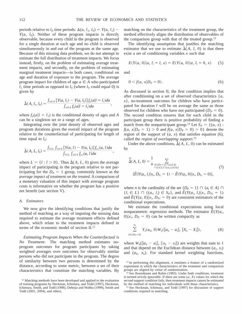
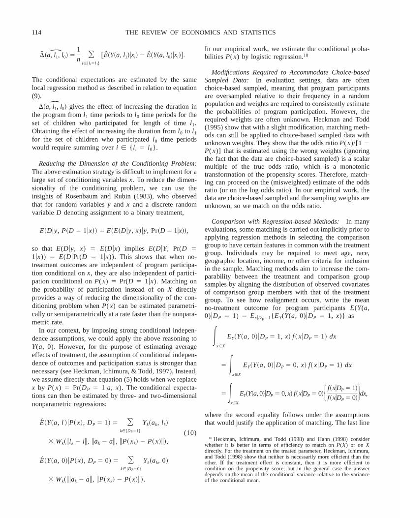
Table 1 shows the sample sizes in groups P, A, and B forthe first and second rounds with and without imposingeligibility on the samples. The first round of data consists of1198 participant (P) children, 1227 A children, and 628 Bchildren interviewed between November 1995 and May1996.23 The second round consists of a follow-up samplefrom the first round and, in addition, a larger sample of newhouseholds that were not visited in the first round. Thesecond round includes 2420 participant children, 2205group A children, and 1732 group B children who wereinterviewed between November 1997 and May 1998. Im-posing the eligibility criteria on the comparison groupsamples leads to a substantial reduction in the samplesizes—roughly cutting them in half. The numbers of chil-dren observed in both rounds are 364 participants in groupP, and 745 group A and 392 group B children.24
B. Eligibility Criteria
To participate in PIDI, families are required to meeteligibility criteria.25 The initial eligibility requirements werethat candidates would be taken who were 6–72 months ofage living in the poor urban communities selected by theprogram according to whether they met the following cri-teria (in order): (1) malnourished children, (2) children withworking parents at risk of lack of supervision, (3) childrenwho had been maltreated, (4) children who lived with onlyone parent or another relative, (5) children with four or moresiblings, and (6) younger children. These criteria were
supposed to be applied lexicographically and were in partsubjective (particularly the first and third), which introducesa random element in who participates in the program, evenafter conditioning on observed characteristics. The initialcriteria subsequently were replaced by a more objectiveeligibility index that awards one point if the family has (a)no running water in the household, (b) no sewer system, (c)no more than two rooms in addition to the bathroom andkitchen in the house, (d) no bathroom or latrine in thehousehold, (e) no separate kitchen, (f) more than fourchildren, (g) a mother with five grades or less of schooling,and (h) an unemployed father. Two points are awarded if (a)the family has only a mother or a father or (b) the mother ofthe family works outside the household. A total of six pointsare required to be eligible for the program. The secondindex has fixed weights rather than the lexicographical oneused initially. It also focuses more on household character-istics and does not include the more subjective aspects ofthe previous one—such as children being malnourished ormaltreated. Nevertheless, in some general sense both theoriginal and the current criteria attempt to identify childrenfrom poor socioeconomic families with limited provision ofhome child care.26
C. Variables
The PIDI data sets provide detailed information on pa-rental, household, and child characteristics. There is infor-mation, for example, on income sources, educational attain-ment, parental occupations, fertility and reproductivehistories, family structure, and possession of durable goods.For all children in the sample households between 6 and 72months of age, there are data on cognitive, psychosocial,and anthropometric test score measures. The outcome mea-sures that we examine in this paper are the following: (i)bulk motor skills, (ii) fine motor skills, (iii) language-auditory skills, (iv) psychosocial skills, (v) height-for-agepercentile, and (vi) weight-for-age percentile.27
23 The sampling frame was a stratified random sample. First PIDI siteswere randomly sampled, and then children within the sites were selectedrandomly.
24 In the first round, there are 1198 children in PIDI. Because ofdifficulties in relocating some of the families, only 739 of these childrenwere followed up in the second round. Of these children, 364 were stillparticipating in PIDI at the time of the second-round data collection, 268were too old for PIDI (had graduated from the program), and 104 were nolonger participating in the program. Thus, we estimate the programdropout rate among the children who were followed in the second roundto be approximately 23%.
25 Once they were determined to be eligible, they could not becomeineligible for the program even if some of their characteristics changedover time.
26 Because of the concern about home supervision, children are morelikely to become eligible for the program if their mothers work, even ifthat implies more family income, ceteris paribus.
27 We also explore whether these are effects on the lower tails of theanthropometric distributions—explicitly, on a height Z score below athreshold of 3 and a weight Z score below a threshold of 2, where thedifferent thresholds reflect the relative severity of the nutritional problemsin this population. (Z scores give the number of standard deviations fromthe mean. They are widely used in the nutrition literature to characterize
TABLE 1.—SAMPLE SIZES OF GROUPS P, A, AND B: ROUNDS 1 AND 2
RoundParticipantSample (P)
Comparison Sample (A) Comparison Sample (B)Participants with Duration*
Without ImposingEligibility
ImposingEligibility
Without ImposingEligibility
ImposingEligibility 0, 1 mo. �2 mo.
1 1198 1227 558 628 333 472 7082 2420 2205 987 1732 963 237 1252Both 364 745 415 392 247 0 268
* The numbers in the last two columns do not sum to the number in the first column, because some observations are missing duration data.
THE REVIEW OF ECONOMICS AND STATISTICS116
The first three are measures of cognitive skills, the fourthis a psychosocial outcome, and the last two are anthropo-metric measures.28 The test score outcomes (i), (ii), (iii), and(iv) are highly significantly correlated with each other, witha statistically significant Kendall tau coefficient of 0.8–0.9for each of the pairwise correlations. Height and weightpercentile measures are less strongly positively correlated(Kendall tau 0.43). Height-for-age percentile is only slightlypositively correlated with the test score outcome measures(with a Kendall tau coefficient equal to 0.06 for each of thetest score measures). The pairwise correlations between theweight-for-age percentile and the test score outcomes are allinsignificantly different from 0.
D. Comparison of Group Mean Characteristics
In table 2, we compare the characteristics of the parentsand of the households for children participating in PIDI(group P) with those of nonparticipating children (in groupsA and B), with and without imposing eligibility on the Aand B samples and with group P subdivided by duration ofprogram participation between 1 month or less and 2months or more.
Panel A of the table compares characteristics of themothers. Approximately 8% of mothers in the PIDI grouphave no education and cannot read or write, which is similarto the rate for mothers in the B sample (eligible and total)but slightly higher than for the A sample (eligible andtotal).29 PIDI mothers are also more likely to participate inthe labor force, but much of this difference is eliminated byimposing program eligibility criteria on samples A and B. Acomparison of the incomes shows that PIDI mothers havelower incomes even though they work on average morehours per day. Among PIDI mothers in the two durationsubsamples (shown in the last two columns) there are nosignificant differences.
Panel B compares characteristics for the fathers. Fathers’educational levels are also lower in the PIDI group than ingroup A (24% with basic or no education, compared to16%) but about the same as in group B (26%). Fathers inthe PIDI group have less stable employment and are morelikely to be employed in occasional work than are fathers inthe other groups; but if the eligibility criteria are applied,there is a reversal in these comparisons. Imposing eligibility
also makes the average income levels similar across groups.Within the P group there are no significant differences forthe two subsamples defined by program duration (last twocolumns).
Panel C compares other characteristics of the householdand reveals differences in family structure across groups:PIDI households are less likely to have both parents residingin the household, and they have lower total household andper capita income. Group differences are reduced substan-tially when the eligibility criteria are imposed.
In summary, in terms of the observed mothers’ , fathers’ ,and other household characteristics, the total A and Bsamples tend to be economically better off than the Psample.30 Applying the eligibility criteria makes the com-parison samples based on A and B much more similar togroup P, though groups A and B still probably on the wholehave more resources. Subdividing the P sample into sub-samples for 1 month and less versus 2 months or greaterduration leads to no significant differences in the subsamplemeans, with the single exception of greater participation inoutside organizations by households with greater duration.
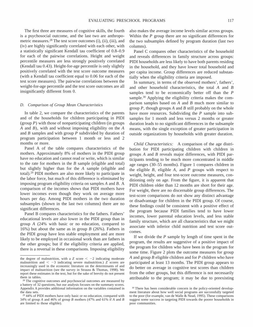
Child Characteristics: A comparison of the age distri-bution for PIDI participating children with children ingroups A and B reveals major differences, with PIDI par-ticipants tending to be much more concentrated in middleage ranges (30–55 months). Figure 1 compares children inthe eligible B, eligible A, and P groups with respect toweight, height, and four test-score outcome measures, con-ditioning only on age. From the figure, it is apparent thatPIDI children older than 12 months are short for their age.For weight, there are no discernable group differences. Thetest-score comparisons do not show any distinct advantageor disadvantage for children in the PIDI group. Of course,these findings could be consistent with a positive effect ofthe program because PIDI families tend to have lowerincomes, lower parental education levels, and less stablefamily structure, which are all characteristics that we mightassociate with inferior child nutrition and test score out-comes.
If we divide the P sample by length of time spent in theprogram, the results are suggestive of a positive impact ofthe program for children who have been in the program forsome time. Figure 2 plots the outcome measures for groupA and group B eligible children and for P children who haveparticipated at least 13 months. The PIDI group appears todo better on average in cognitive test scores than childrenfrom the other groups, but this difference is not necessarilyattributable to the program; it may be due to preexisting
the degree of malnutrition, with a Z score � �2 indicating moderatemalnutrition and � �3 indicating severe malnutrition.) Z scores areincreasingly used in the economic literature on the determinants of andimpact of malnutrition (see the survey in Strauss & Thomas, 1998). Wereport these estimates in the text, but for the sake of brevity do not presentthem in tables.
28 The cognitive outcomes and psychosocial outcomes are measured bya battery of 32 questions, but our analysis focuses on the summary scores.Appendix A provides additional information on the variables contained inthe data sets.
29 44% of PIDI mothers have only basic or no education, compared with34% of group A and 46% of group B mothers (47% and 61% if A and Bare limited to those eligible).
30 There has been considerable concern in the policy-oriented develop-ment literature about how well social programs are successfully targetedto the poor (for example, van de Walle & Nead, 1995). These comparisonssuggest some success in targeting PIDI towards the poorer households inpoor communities.
EVALUATING PRESCHOOL PROGRAMS 117

TABLE 2.—COMPARISON OF GROUP MEAN CHARACTERISTICS
CharacteristicParticipants’Sample (P)
Eligible Nonpart. Sample Eligibility Not Imposed Participants with Duration
A B A B �1 mo. �1 mo.
A. Comparison of Mothers’ Characteristics in Participant and Eligible Nonparticipant Samples*
Education:None 8.48 5.49 8.17 0.88 1.60 8.37 8.81Preschool 0.04 0.00 0.00 0.04 0.25 0 0.15Basic 35.53 41.45 52.99 15.45 24.37 35.74 34.93Middle school 21.48 24.25 20.13 18.89 21.08 21.11 22.54Secondary 28.40 22.23 14.15 42.89 37.44 29.63 24.93Normal school 1.56 1.83 2.20 2.34 3.88 1.42 1.94University 1.98 2.56 1.57 13.55 6.66 1.68 2.84Technical 2.53 2.10 0.79 4.28 3.20 2.05 3.88Other or no ans. 0.00 0.09 0.00 1.68 1.52 0.00 0.00
Age:Mean 29.04 30.28 30.97 33.17 33.84 29.16 28.71(s.d.) (6.34) (6.92) (7.34) (7.80) (8.86) (6.43) (6.07)
Literacy:Can read/write 92.02 94.78 91.82 99.34 98.40 92.00 92.09Cannot read/write 7.98 5.22 8.18 0.66 1.60 8.00 7.91
Type of work:Permanent 67.16 59.10 59.91 77.05 75.97 67.47 66.27Occasional 19.65 22.14 20.44 19.68 11.98 19.95 18.81No job 13.19 18.76 19.65 3.27 4.05 12.58 14.92
Kind of job:Worker 7.04 5.74 7.63 24.95 27.77 6.98 7.19Clerical 55.45 23.76 19.77 41.01 35.68 57.19 50.35Self-employed 34.33 61.60 65.95 29.65 33.22 32.81 38.77Employer 0.09 0.79 0.78 4.01 2.90 0.07 0.35Family business 2.82 8.11 5.68 0.27 0.44 2.71 3.16Other 0.27 0.00 0.20 0.09 0.00 0.30 0.18
Hours worked/day:Mean 8.70 7.70 7.88 9.19 9.28 8.72 8.63(s.d.) (2.62) (3.18) (3.29) (2.43) (2.51) (2.56) (2.79)
Income/month:Mean 328.50 443.14 496.20 907.26 858.29 329.78 324.73(s.d.) (427.32) (518.02) (689.96) (948.54) (934.46) (461.15) (306.77)
B. Comparison of Fathers’ Characteristics in Participant and Eligible Nonparticipant Samples*
Education:None 1.97 1.45 1.94 0.88 1.60 2.14 1.48Preschool 0.00 1.21 0.39 0.04 0.25 0.00 0.00Basic 21.91 21.23 33.33 15.45 24.37 21.18 23.99Middle school 22.44 27.14 25.19 18.89 21.08 22.47 22.32Secondary 42.81 41.74 31.59 42.89 37.44 43.65 40.41Normal school 1.77 1.45 2.91 2.34 3.88 1.94 1.29University 5.13 3.38 2.71 13.55 6.66 4.47 7.01Technical 3.02 2.29 1.74 4.28 3.20 3.11 2.77Other or no ans. 0.96 1.33 0.20 1.68 1.52 1.04 0.74
Literacy:Can read/write 98.32 99.03 98.06 99.34 98.40 98.12 98.89Cannot read/write 1.68 0.97 1.94 0.66 1.60 1.88 1.11
Age:Mean 32.52 33.78 34.78 33.17 33.84 32.56 32.39(s.d.) (7.79) (8.01) (8.93) (7.80) (8.86) (7.80) (7.76)
Type of work:Permanent 71.33 72.50 73.06 77.05 75.97 71.05 72.14Occasional 25.36 23.28 20.35 19.68 11.98 25.91 23.80No job 3.31 4.22 6.59 3.27 4.05 3.04 4.06
Kind of job:Worker 37.48 29.97 28.63 24.95 27.77 36.41 40.58Clerical 33.52 32.49 27.80 41.01 35.68 34.74 30.00Self-employed 26.18 33.75 40.25 29.65 33.22 26.25 25.96Employer 2.58 3.78 2.28 4.01 2.90 2.34 3.27Family business 0.10 0.00 1.04 0.27 0.44 0.13 0.00Other 0.15 0.00 0.00 0.09 0.00 0.13 0.19
Hours worked/day:Mean 9.51 9.57 9.54 9.19 9.28 9.51 9.52(s.d.) (2.35) (2.47) (2.62) (2.43) (2.51) (2.36) (2.31)
Income/month:Mean 713.40 745.21 737.95 907.26 858.29 711.82 717.99(s.d.) (906.67) (662.84) (556.31) (948.54) (934.46) (1011.26) (490.96)
C. Comparison of Households’ Characteristics in Participant and Eligible Nonparticipant Samples*
Family structure:Only father resides in house 1.74 0.27 0.77 0.19 0.37 1.59 2.15Only mother resides in house 20.02 24.16 19.20 15.30 11.38 19.84 20.52Neither parent resides in house 1.21 0.81 1.54 0.57 0.96 1.03 1.72Both parents reside in house 77.04 74.75 78.49 86.13 87.29 77.55 75.61
Household income:Mean 902.65 1019.65 1070.33 1189.61 1131.65 900.91 907.87(s.d.) (994.37) (1028.33) (1025.64) (1429.10) (1239.67) (1083.12) (685.25)
Per person income:Mean 185.18 200.77 201.22 242.00 217.75 183.49 190.25(s.d.) (233.10) (299.72) (206.34) (346.42) (251.58) (256.71) (147.67)
Number of persons in household:Mean 5.23 5.68 5.75 5.39 5.53 5.23 5.24(s.d.) (1.92) (2.26) (2.06) (2.05) (2.03) (1.91) (1.93)
Number of rooms in household:Mean 1.61 1.68 1.66 1.95 1.94 1.62 1.56(s.d.) (1.08) (0.99) (0.93) (1.27) (1.27) (1.07) (1.09)
Household ownership:Own house 35.24 30.23 44.24 30.78 42.35 35.29 35.07Rented house 33.67 30.68 24.58 27.66 24.39 34.10 32.46Paid in kind or relative’s house 27.69 34.57 28.88 35.47 29.93 27.28 28.84Other 3.41 4.52 2.31 6.09 3.33 3.33 3.6
Household has a TVMean 0.31 0.37 0.31 0.50 0.42 0.31 0.32(s.d.) (0.46) (0.48) (0.46) (0.50) (0.49) (0.47) (0.45)
Participation in outside org.† 58.41 25.15 36.80 27.71 31.89 61.98 48.06
* Includes both rounds of data, but excludes observations from second round who were also included in first round.† Someone in household participates in neighborhood organizations.
THE REVIEW OF ECONOMICS AND STATISTICS118
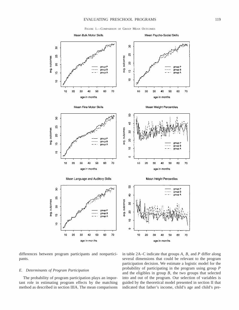
differences between program participants and nonpartici-pants.
E. Determinants of Program Participation
The probability of program participation plays an impor-tant role in estimating program effects by the matchingmethod as described in section IIIA. The mean comparisons
in table 2A–C indicate that groups A, B, and P differ alongseveral dimensions that could be relevant to the programparticipation decision. We estimate a logistic model for theprobability of participating in the program using group Pand the eligibles in group B, the two groups that selectedinto and out of the program. Our selection of variables isguided by the theoretical model presented in section II thatindicated that father’s income, child’s age and child’s pre-
FIGURE 1.—COMPARISON OF GROUP MEAN OUTCOMES
EVALUATING PRESCHOOL PROGRAMS 119
program quality status are potential determinants of partic-ipation.31 Information is available on all these variables,except preprogram quality (see discussion below). We selectthe particular set of included regressors for the logistic
model from those shown in table 2 to maximize the per-centage correctly classified by the hit-or-miss criterion.Under the resulting model, 79% of the observations arecorrectly classified.32 The included regressors are listed inappendix C. The most useful predictors of participation are
31 Mother’s labor force participation was not included in the participa-tion model out of concern that it might change in response to treatment.The model of section II assumes that the mother’s labor force participationis jointly determined with the participation decision.
32 77% of the participants and 84% of the controls are correctly classi-fied.
FIGURE 2.—COMPARISON OF GROUP MEAN OUTCOMES, DURATION AT LEAST 13 MONTHS
THE REVIEW OF ECONOMICS AND STATISTICS120
(i) presence of a mother in the household, (ii) educationlevel of the mother, (iii) number of children, (iv) educa-tion level of the father, and (v) monthly income of thefather.
For group A, it is impossible to know which familieswould have elected to participate in the program had theprogram been available to them. However, under the as-sumption that the same participation process governs deci-sions for group A as for group B, we can impute probabil-ities of participation for group A families using the
coefficients from the participation model that was estimatedon groups P and B.33
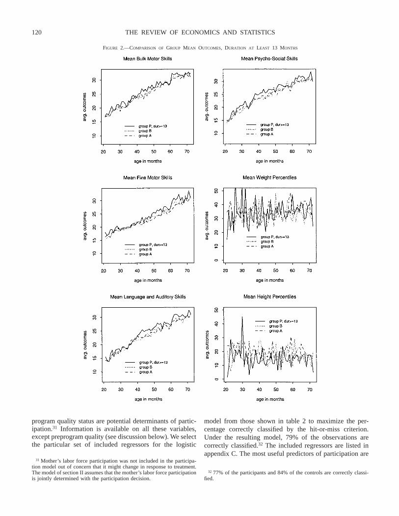
The first column of figure 3 plots the log odds ratio forparticipating children and for eligible children in the B andA groups. For groups P and B the supports of the log oddsratios overlap, but if group A is used as a comparison group,
33 This requires assuming that there are no significant unobservedlocality characteristics affecting outcomes, so that a similar model forparticipation for groups P and B can also be applied to group A.
FIGURE 3.—DISTRIBUTION OF ESTIMATED LOG ODDS RATIO
EVALUATING PRESCHOOL PROGRAMS 121
some high values of the log odds ratio are observed forprogram participants for which no matching values can befound for children in the A group. This limits the range ofvalues over which treatment impacts can be estimated.
Our estimates of the marginal effects of longer durationsin the program are based on the survival probability corre-sponding to the probability that duration in the program is 2months or more.34 Appendix C lists of set of regressors weused for this model (chosen using the hit-or-miss criterionwith a correct classification rate of 76%). The log odds ratioof the survival probabilities is plotted in the second columnof figure 3.35
F. Impacts Estimated by Traditional Regression Methods
Before presenting impact estimates based on the match-ing estimators, we first report for comparison estimates thatare obtained by simple regression estimators. First, weestimate a simple cross-sectional regression model for thethree cognitive development tests, the psychosocial abilitytest, and the two anthropometric indicators, based on thecombined P and eligible B samples. Our specification in-cludes as independent variables a dichotomous variable forparticipation in PIDI, a cubic in duration in PIDI, a cubic inthe child’s age, the child’s sex, and a set of conditioningvariables that is the same as used in estimating the proba-bility of program participation, as described in the previoussection.36 Figure 4 plots the estimated program impact as afunction of duration in the program.
The figure shows that estimated program impacts on testscores are mostly positive and on the order of one additionalanswer correct (out of a possible 32). For the anthropomet-ric outcomes, we find the counterintuitive result of a nega-tive impact of the program on weight and on height. We donot find these estimates to be credible, because large nega-tive impacts of the program on anthropometrics immedi-ately upon program entry (as indicated by the estimatednegative impact of PIDI participation on the intercept) areextremely unlikely, which suggests that the regression mod-els may be misspecified. One potential source of misspeci-fication is that program impacts may depend in a nonaddi-tive way on age and program duration. The matchingestimators described below nonparametrically estimate thenature of the dependence.
We also consider estimates based on a DID estimator forthe much smaller subset of children who are observed inboth sample rounds in P and in eligible group B (see table2 for sample sizes, and appendix E, table E2, for thecoefficient estimates). The estimates are imprecise due tothe substantially reduced sample sizes. In this case, theestimates suggest that the effects of the program are nega-tive for all outcomes except the height-for-age percentile(see figure 5).
G. Cumulative Impacts Estimated by the Method ofMatching
We next describe estimated cumulative program impactsbased on the matching estimators developed in section III,first conditional on age only and then conditional on bothage and duration in the program. We also present results onthe marginal impacts. In implementing the matching esti-mators, we choose bandwidth values by the least squarescross-validation (LSCV) method, which searches over agrid of possible bandwidth values and chooses the valuesthat minimize the integrated squared error of the nonpara-metric estimators.37
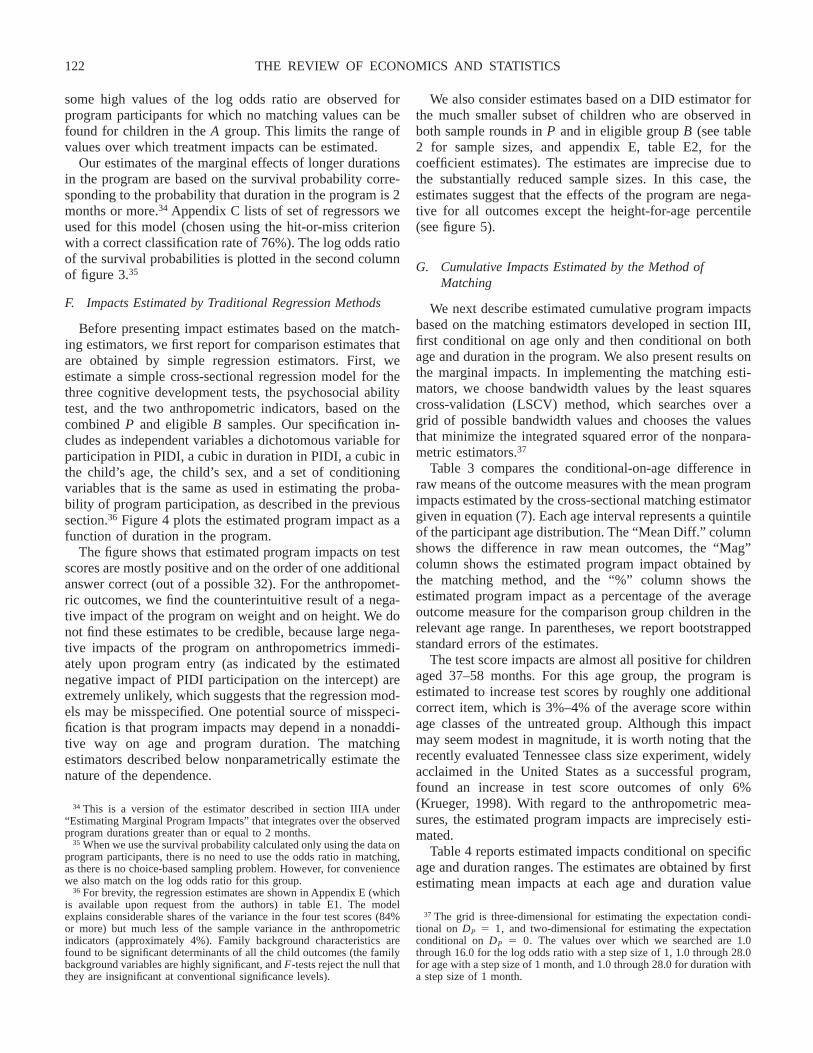
Table 3 compares the conditional-on-age difference inraw means of the outcome measures with the mean programimpacts estimated by the cross-sectional matching estimatorgiven in equation (7). Each age interval represents a quintileof the participant age distribution. The “Mean Diff.” columnshows the difference in raw mean outcomes, the “Mag”column shows the estimated program impact obtained bythe matching method, and the “%” column shows theestimated program impact as a percentage of the averageoutcome measure for the comparison group children in therelevant age range. In parentheses, we report bootstrappedstandard errors of the estimates.
The test score impacts are almost all positive for childrenaged 37–58 months. For this age group, the program isestimated to increase test scores by roughly one additionalcorrect item, which is 3%–4% of the average score withinage classes of the untreated group. Although this impactmay seem modest in magnitude, it is worth noting that therecently evaluated Tennessee class size experiment, widelyacclaimed in the United States as a successful program,found an increase in test score outcomes of only 6%(Krueger, 1998). With regard to the anthropometric mea-sures, the estimated program impacts are imprecisely esti-mated.
Table 4 reports estimated impacts conditional on specificage and duration ranges. The estimates are obtained by firstestimating mean impacts at each age and duration value
34 This is a version of the estimator described in section IIIA under“Estimating Marginal Program Impacts” that integrates over the observedprogram durations greater than or equal to 2 months.
35 When we use the survival probability calculated only using the data onprogram participants, there is no need to use the odds ratio in matching,as there is no choice-based sampling problem. However, for conveniencewe also match on the log odds ratio for this group.
36 For brevity, the regression estimates are shown in Appendix E (whichis available upon request from the authors) in table E1. The modelexplains considerable shares of the variance in the four test scores (84%or more) but much less of the sample variance in the anthropometricindicators (approximately 4%). Family background characteristics arefound to be significant determinants of all the child outcomes (the familybackground variables are highly significant, and F-tests reject the null thatthey are insignificant at conventional significance levels).
37 The grid is three-dimensional for estimating the expectation condi-tional on DP 1, and two-dimensional for estimating the expectationconditional on DP 0. The values over which we searched are 1.0through 16.0 for the log odds ratio with a step size of 1, 1.0 through 28.0for age with a step size of 1 month, and 1.0 through 28.0 for duration witha step size of 1 month.
THE REVIEW OF ECONOMICS AND STATISTICS122

observed in the data and then taking averages over theindividual impacts within each age-duration class.38 Theresults indicate that average impacts increase as length ofexposure to treatment increases. Impacts are almost alwayspositive for children who have participated in the programfor at least 13 months (with only two exceptions, both forchildren under 36 months old who have participated 25�months) and roughly twice the order of magnitude of theoverall average impacts reported in table 3. They tend to belarger than those found under the cubic specification of
section IV C. The bottom two panels of table 4 show resultsfor the anthropometric measures, which are insignificantlydifferent from 0.
We carried out a similar analysis using as a source ofcomparison group data the sample of children living in ageographic area not served by the program (group A de-scribed in section II). Tables 5 and 6 report the estimatedprogram impacts in a format identical to the previous twotables. The impact estimates on test scores are generallypositive over all age ranges for durations of exposure of atleast 7 months. The estimates are more widely statisticallysignificant for the A comparison group than for the B group;
38 Averages are therefore self-weighting by the joint duration and agedensity.
FIGURE 4.—ESTIMATED PROGRAM IMPACTS FROM CROSS-SECTIONAL, CUBIC-IN-DURATION MODEL, SAMPLES P AND B
EVALUATING PRESCHOOL PROGRAMS 123

they are significant over half the time for children aged 36months or less, and almost always for children aged 59�months. With regard to the anthropometric measures, wefind statistically significant negative impacts on weight forshort durations of exposure. We think it unlikely that theprogram could decrease children’s weight over a short timeinterval by as much as estimated. Rather, the estimatednegative impacts on weight are probably evidence of biasarising from selection into the program on unobservablesthat is not taken into account by matching. An importantunobservable is preprogram nutritional status, on which, asnoted in section IV B, the initial program eligibility criteriaplaced primary emphasis.
H. Marginal Program Impacts Estimated by the Methodof Matching
Because preprogram nutritional status represents an im-portant unobservable, our preferred estimates are those forthe marginal impact of the program for different durationsof participation obtained using only data for program par-ticipants (P). These estimates use participants with shorterdurations as the comparison group for participants withlonger durations and use matching to control for differencesin child characteristics that affect the program durationrather than the participation decision. As described insection IIIA, the marginal estimator allows selectivity into
FIGURE 5.—ESTIMATED PROGRAM IMPACTS BASED ON DIFFERENCE-IN-DIFFERENCES MODEL, SAMPLES P AND B
THE REVIEW OF ECONOMICS AND STATISTICS124

TABLE 3.—COMPARISON OF DIFFERENCE IN RAW MEANS AND CUMULATIVE MEAN PROGRAM IMPACTS AFTER ADJUSTING FOR SELECTIVITY
INTO THE PROGRAM USING MATCHING METHOD—SAMPLES P AND B
Outcome
Age: 6–24 25–36 37–41 42–58 59� mo.
MeanDiff.
ImpactMeanDiff.
ImpactMeanDiff.
ImpactMeanDiff.
ImpactMeanDiff.
Impact
Mag. % Mag. % Mag. % Mag. % Mag. %
Bulk motor skills 2.17 �0.03 �0 0.33 �0.04 �0 0.60 0.80 3 0.56 0.85 3 0.09 0.00 0(0.21) (0.29) (0.24) (0.22) (0.29)
Fine motor skills 2.43 0.34 3 0.23 0.12 1 0.12 0.33 2 0.76 0.52 2 0.23 �0.05 �0(0.17) (0.27) (0.11) (0.22) (0.40)
Language 1.56 �0.02 �0 0.16 �0.19 �1 1.00 0.73 3 0.78 0.76 3 0.28 0.16 1(0.17) (0.33) (0.24) (0.30) (0.29)
Psychosocial 1.85 �0.40 �4 0.68 0.03 0 1.10 1.35 6 0.74 0.53 2 0.24 �0.30 �1(0.28) (0.41) (0.34) (0.23) (0.35)
Weight perc. �3.8 �3.2 �10 �2.9 �0.36 �1 �5.3 0.40 1 0.41 0.74 2 2.20 �1.6 �5(3.99) (2.03) (1.64) (1.40) (1.97)
Height perc. �2.7 2.55 13 �2.5 1.22 7 �4.6 �0.59 �3 �0.36 �0.85 �5 �3.6 0.38 2(3.12) (1.72) (1.76) (1.39) (2.28)
Bootstrapped standard errors in parentheses.
TABLE 4.—ESTIMATED CUMULATIVE IMPACTS BY DURATION AND AGE CLASSES—SAMPLES P AND B
Age inMonths Duration 1–6 7–12 13–18 19–24 25� mo.
Bulk Motor Skills
6–24 �0.05 (�0%) 0.04 (0%) 0.09 (1%) � �25–36 �0.43 (�2%) �0.06 (�0%) 0.72 (4%)* 0.99 (5%)* 0.36 (2%)37–41 0.40 (2%) 0.82 (3%)* 1.32 (6%)* 1.41 (6%)* 1.20 (5%)*42–58 0.31 (1%) 1.02 (4%)* 1.39 (5%)* 1.12 (4%)* 1.54 (6%)*59� �0.49 (�2%) 0.38 (1%) 0.32 (1%) 0.35 (1%) 0.43 (1%)
Fine Motor Skills
6–24 0.27 (2%) 0.45 (4%) 0.87 (7%)* � �25–36 0.02 (0%) 0.10 (1%) 0.40 (2%) 0.35 (2%) �0.24 (�1%)37–41 0.29 (1%) 0.34 (2%)* 0.53 (2%)* 0.40 (2%)* 0.09 (0%)42–58 0.03 (0%) 0.81 (3%)* 1.05 (4%)* 0.73 (3%)* 0.98 (4%)*59� �0.80 (�3%) 0.38 (1%) 0.59 (2%) 0.53 (2%) 0.57 (2%)
Language and Auditory Skills
6–24 �0.11 (�1%) 0.27 (2%) 0.22 (2%) � �25–36 �0.48 (�3%) 0.01 (0%) 0.25 (1%) 0.34 (2%) �0.71 (�4%)37–41 0.36 (2%) 1.19 (6%)* 1.42 (7%)* 0.95 (4%)* 0.42 (2%)42–58 �0.09 (�0%) 1.12 (5%)* 1.65 (7%)* 1.38 (6%)* 1.54 (6%)*59� �0.76 (�3%)* 0.77 (3%)* 0.69 (2%)* 1.26 (4%)* 0.68 (2%)
Psychosocial Skills
6–24 �0.49 (�4%)* �0.18 (�2%) 0.01 (0%) � �25–36 �0.57 (�3%) 0.11 (1%) 0.83 (4%)* 1.72 (9%)* 1.51 (8%)*37–41 0.59 (3%) 1.43 (6%)* 2.09 (9%)* 2.51 (11%)* 2.35 (10%)*42–58 0.00 (0%) 0.75 (3%)* 1.05 (4%)* 0.81 (3%)* 1.15 (4%)*59� �1.11 (�4%)* 0.10 (0%) 0.15 (1%) 0.56 (2%) 0.53 (2%)
Weight Percentile
6–12 �4.10 (�13%) �1.58 (�5%) 0.13 (0%) � �13–18 �1.72 (�5%) 0.20 (1%) 1.02 (3%) 2.38 (7%) 3.61 (11%)19–24 �0.84 (�2%) 0.65 (2%) 1.38 (4%) 2.00 (5%) 2.87 (8%)25–30 �0.84 (�3%) 1.13 (3%) 1.57 (5%) 1.73 (5%) 3.43 (10%)31–36 �3.56 (�11%) �0.66 (�2%) �0.18 (�1%) 0.28 (1%) �0.17 (�1%)
Height Percentile
6–12 2.63 (13%) 2.68 (14%) 1.59 (8%) � �13–18 1.80 (10%) 1.36 (8%) 0.76 (4%) 0.24 (1%) �0.93 (�5%)19–24 �0.02 (�0%) �0.33 (�2%) �1.04 (�5%) �1.15 (�5%) �1.52 (�7%)25–30 �0.37 (�2%) �0.63 (�4%) �1.08 (�7%) �1.46 (�9%) �1.35 (�9%)31–36 �0.31 (�2%) 0.92 (5%) 1.09 (6%) 0.86 (5%) �0.20 (�1%)
* Significant at the 10% level.Percentage impact shown in parentheses.
EVALUATING PRESCHOOL PROGRAMS 125
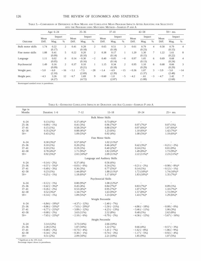
TABLE 5.—COMPARISON OF DIFFERENCE IN RAW MEANS AND CUMULATIVE MEAN PROGRAM IMPACTS AFTER ADJUSTING FOR SELECTIVITY
INTO THE PROGRAM USING MATCHING METHOD—SAMPLES P AND A
Outcome
Age: 6–24 25–36 37–41 42–58 59� mo.
MeanDiff.
ImpactMeanDiff.
ImpactMeanDiff.
ImpactMeanDiff.
ImpactMeanDiff.
Impact
Mag. % Mag. % Mag. % Mag. % Mag. %
Bulk motor skills 1.74 0.22 2 0.41 0.28 2 0.65 0.51 3 0.61 0.79 4 0.58 0.79 4(0.17) (0.18) (0.18) (0.23) (0.15)
Fine motor skills 1.88 0.41 5 0.22 0.20 2 0.38 0.17 1 1.20 1.30 7 1.22 1.61 8(0.09) (0.10) (0.14) (0.15) (0.22)
Language 1.11 0.02 0 0.14 �0.30 �2 0.40 �0.05 �0 0.97 1.05 6 0.69 0.68 4(0.05) (0.16) (0.14) (0.13) (0.24)
Psychosocial 1.49 0.16 2 0.37 0.10 1 1.15 0.34 2 0.95 1.10 6 0.68 0.66 3(0.09) (0.21) (0.18) (0.29) (0.29)
Weight perc. �5.0 �6.0 �16 �5.1 �7.5 �28 �1.4 �4.9 �15 �0.36 1.07 3 �3.9 �5.0 �14(2.10) (2.69) (2.39) (1.37) (2.48)
Height perc. �4.3 3.26 12 �6.7 1.69 9 �0.60 �1.0 �5 �4.2 �.61 �3 �4.7 1.42 7(4.27) (4.72) (2.87) (1.88) (2.68)
Bootstrapped standard errors in parentheses.
TABLE 6.—ESTIMATED CUMULATIVE IMPACTS BY DURATION AND AGE CLASSES—SAMPLES P AND A
Age inMonths Duration: 1–6 7–12 13–18 19–24 25� mo.
Bulk Motor Skills
6–24 0.13 (1%) 0.37 (4%)* 0.73 (8%)* � �25–36 �0.09 (�1%) 0.41 (3%) 0.96 (7%)* 0.97 (7%)* 0.07 (1%)37–41 0.15 (1%) 0.58 (3%)* 0.88 (5%)* 0.97 (6%)* 1.07 (6%)*42–58 0.35 (2%)* 0.88 (4%)* 1.23 (6%) 1.10 (6%)* 1.42 (7%)*59� 0.43 (2%) 1.09 (5%)* 0.92 (4%) 1.08 (5%)* 1.19 (6%)*
Fine Motor Skills
6–24 0.30 (3%)* 0.57 (6%)* 1.02 (11%)* � �25–36 0.10 (1%) 0.20 (2%) 0.46 (4%)* 0.42 (3%)* �0.21 (�2%)37–41 0.10 (1%) 0.19 (1%) 0.40 (2%)* 0.24 (1%) 0.01 (0%)42–58 0.78 (4%)* 1.71 (9%)* 1.82 (10%)* 1.49 (8%)* 1.73 (9%)*59� 0.92 (5%)* 2.02 (10%)* 2.09 (11%)* 2.22 (11%)* 2.23 (11%)*
Language and Auditory Skills
6–24 �0.14 (�2%) 0.37 (4%) 0.56 (6%) � �25–36 �0.57 (�5%)* �0.03 (�0%) 0.24 (2%) �0.21 (�2%) �0.98 (�8%)*37–41 �0.49 (�3%) 0.36 (3%) 0.77 (5%)* 0.14 (1%) �0.12 (�1%)42–58 0.23 (1%) 1.44 (8%)* 1.88 (11%)* 1.72 (10%)* 1.74 (10%)*59� �0.25 (�1%) 1.18 (6%)* 1.17 (6%)* 1.83 (10%)* 1.35 (7%)*
Psychosocial Skills
6–24 �0.12 (�1%) 0.80 (9%)* 1.08 (12%)* � �25–36 �0.42 (�3%)* 0.45 (4%) 0.84 (7%)* 0.83 (7%)* 0.09 (1%)37–41 �0.26 (�2%) 0.53 (4%)* 0.95 (7%)* 1.07 (7%)* 1.10 (7%)*42–58 0.52 (3%)* 1.34 (7%)* 1.63 (9%)* 1.57 (8%)* 1.72 (9%)*59� �0.14 (�1%) 1.09 (5%)* 1.23 (6%)* 1.43 (7%)* 1.29 (6%)*
Weight Percentile
6–24 �6.84 (�19%)* �4.37 (�12%) �2.40 (�7%) � �25–36 �8.86 (�33%)* �7.63 (�29%)* �5.50 (�21%) �4.86 (�18%) �0.08 (�0%)37–41 �6.77 (�21%)* �3.89 (�12%) �4.23 (�13%) �3.46 (�11%) 1.06 (3%)42–58 �0.68 (�2%) 3.63 (11%) 2.52 (8%) 0.48 (1%) 2.62 (8%)59� �7.65 (�22%)* �2.10 (�6%) �0.79 (�2%) �4.36 (�12%) �5.67 (�16%)
Height Percentile
6–24 3.14 (12%) 3.73 (14%) 2.66 (10%) � �25–36 2.28 (12%) 1.87 (10%) 1.22 (7%) 0.66 (4%) �0.57 (�3%)37–41 �0.48 (�2%) �0.73 (�4%) �1.41 (�7%) �1.62 (�8%) �1.86 (�9%)42–58 �0.34 (�2%) �0.30 (�1%) �0.74 (�3%) �1.17 (�5%) �0.92 (�4%)59� 0.51 (2%) 2.09 (10%) 2.21 (10%) 1.85 (9%) 1.07 (5%)
* Significant at the 10% level.Percentage impact shown in parentheses.
THE REVIEW OF ECONOMICS AND STATISTICS126
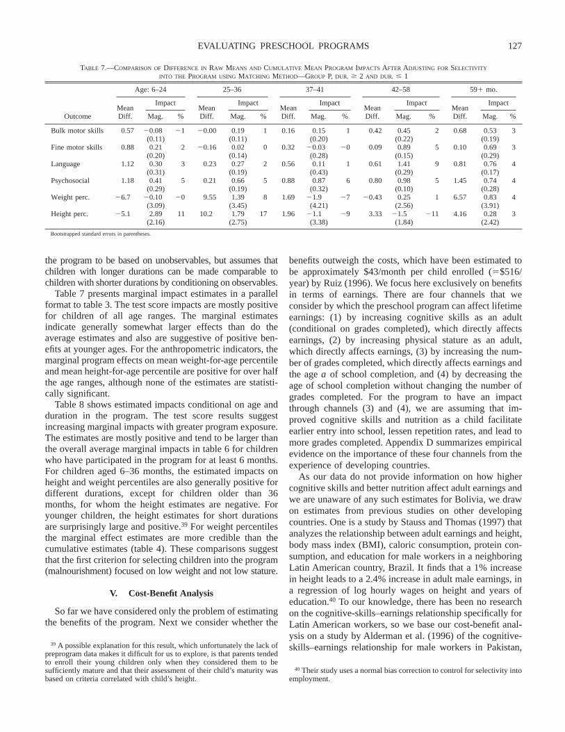
the program to be based on unobservables, but assumes thatchildren with longer durations can be made comparable tochildren with shorter durations by conditioning on observables.
Table 7 presents marginal impact estimates in a parallelformat to table 3. The test score impacts are mostly positivefor children of all age ranges. The marginal estimatesindicate generally somewhat larger effects than do theaverage estimates and also are suggestive of positive ben-efits at younger ages. For the anthropometric indicators, themarginal program effects on mean weight-for-age percentileand mean height-for-age percentile are positive for over halfthe age ranges, although none of the estimates are statisti-cally significant.
Table 8 shows estimated impacts conditional on age andduration in the program. The test score results suggestincreasing marginal impacts with greater program exposure.The estimates are mostly positive and tend to be larger thanthe overall average marginal impacts in table 6 for childrenwho have participated in the program for at least 6 months.For children aged 6–36 months, the estimated impacts onheight and weight percentiles are also generally positive fordifferent durations, except for children older than 36months, for whom the height estimates are negative. Foryounger children, the height estimates for short durationsare surprisingly large and positive.39 For weight percentilesthe marginal effect estimates are more credible than thecumulative estimates (table 4). These comparisons suggestthat the first criterion for selecting children into the program(malnourishment) focused on low weight and not low stature.
V. Cost-Benefit Analysis
So far we have considered only the problem of estimatingthe benefits of the program. Next we consider whether the
benefits outweigh the costs, which have been estimated tobe approximately $43/month per child enrolled ($516/year) by Ruiz (1996). We focus here exclusively on benefitsin terms of earnings. There are four channels that weconsider by which the preschool program can affect lifetimeearnings: (1) by increasing cognitive skills as an adult(conditional on grades completed), which directly affectsearnings, (2) by increasing physical stature as an adult,which directly affects earnings, (3) by increasing the num-ber of grades completed, which directly affects earnings andthe age a of school completion, and (4) by decreasing theage of school completion without changing the number ofgrades completed. For the program to have an impactthrough channels (3) and (4), we are assuming that im-proved cognitive skills and nutrition as a child facilitateearlier entry into school, lessen repetition rates, and lead tomore grades completed. Appendix D summarizes empiricalevidence on the importance of these four channels from theexperience of developing countries.
As our data do not provide information on how highercognitive skills and better nutrition affect adult earnings andwe are unaware of any such estimates for Bolivia, we drawon estimates from previous studies on other developingcountries. One is a study by Stauss and Thomas (1997) thatanalyzes the relationship between adult earnings and height,body mass index (BMI), caloric consumption, protein con-sumption, and education for male workers in a neighboringLatin American country, Brazil. It finds that a 1% increasein height leads to a 2.4% increase in adult male earnings, ina regression of log hourly wages on height and years ofeducation.40 To our knowledge, there has been no researchon the cognitive-skills–earnings relationship specifically forLatin American workers, so we base our cost-benefit anal-ysis on a study by Alderman et al. (1996) of the cognitive-skills–earnings relationship for male workers in Pakistan,39 A possible explanation for this result, which unfortunately the lack of
preprogram data makes it difficult for us to explore, is that parents tendedto enroll their young children only when they considered them to besufficiently mature and that their assessment of their child’s maturity wasbased on criteria correlated with child’s height.
40 Their study uses a normal bias correction to control for selectivity intoemployment.
TABLE 7.—COMPARISON OF DIFFERENCE IN RAW MEANS AND CUMULATIVE MEAN PROGRAM IMPACTS AFTER ADJUSTING FOR SELECTIVITY
INTO THE PROGRAM USING MATCHING METHOD—GROUP P, DUR. � 2 AND DUR. � 1
Outcome
Age: 6–24 25–36 37–41 42–58 59� mo.
MeanDiff.
ImpactMeanDiff.
ImpactMeanDiff.
ImpactMeanDiff.
ImpactMeanDiff.
Impact
Mag. % Mag. % Mag. % Mag. % Mag. %
Bulk motor skills 0.57 �0.08 �1 �0.00 0.19 1 0.16 0.15 1 0.42 0.45 2 0.68 0.53 3(0.11) (0.11) (0.20) (0.22) (0.19)
Fine motor skills 0.88 0.21 2 �0.16 0.02 0 0.32 �0.03 �0 0.09 0.89 5 0.10 0.69 3(0.20) (0.14) (0.28) (0.15) (0.29)
Language 1.12 0.30 3 0.23 0.27 2 0.56 0.11 1 0.61 1.41 9 0.81 0.76 4(0.31) (0.19) (0.43) (0.29) (0.17)
Psychosocial 1.18 0.41 5 0.21 0.66 5 0.88 0.87 6 0.80 0.98 5 1.45 0.74 4(0.29) (0.19) (0.32) (0.10) (0.28)
Weight perc. �6.7 �0.10 �0 9.55 1.39 8 1.69 �1.9 �7 �0.43 0.25 1 6.57 0.83 4(3.09) (3.45) (4.21) (2.56) (3.91)
Height perc. �5.1 2.89 11 10.2 1.79 17 1.96 �1.1 �9 3.33 �1.5 �11 4.16 0.28 3(2.16) (2.75) (3.38) (1.84) (2.42)
Bootstrapped standard errors in parentheses.
EVALUATING PRESCHOOL PROGRAMS 127
which finds that a 1% increase in cognitive skills increasesearnings by 0.23%.41 Their study has an advantage oversome other studies in the literature in that it controls for thepotential endogeneity of cognitive ability in the wage equa-tion. As we only observe the children in our study at a veryyoung age, we assume for the cost-benefit analysis thatincreases in height and cognitive ability as a child have apersistent effect and translate into equiproportional in-creases as an adult.42,43
The present discounted value of earnings associated witha 1% increase in height is calculated as follows. Let y(s, c,h) be the annual earnings of individuals with s gradescompleted, cognitive ability c, and height h, and let a be theage of completing school. We draw a distinction betweengrades completed and rate of progression through grades,because a number of students in Bolivia both start schoollate and repeat grades. Estimates from the 1990 third roundof the Encuesta Integrada de Hogares (Integrated House-hold Survey), which covers the ten most populous urbanareas in Bolivia, indicate that for 16-year-olds in urbanBolivia the gap in grades completed due to factors such aslate starting and grade repetition was 10%–16% of thegrades actually completed, or between 0.9 and 1.4 grades, incomparison with a mean of 8.6 grades actually completed.
41 Their study finds that a 7.3% increase in cognitive skills, evaluated atthe mean, leads to a 1.3% increase in earnings, conditional on years ofschooling. We have converted their estimates to the gain expected from a1% increase in skills.
42 Measures of intelligence have been found to be highly correlated acrossages. For example, the Berkeley Growth Study found a correlation of 0.71between test scores measured at ages 4 and 17 (Currie & Thomas, 1999).
43 We use height for our illustration rather than BMI because thisassumption is more dubious for BMI than for height. But, as noted below,we consider a small percentage increase in height in comparison withthose obtained for some of the estimators in section IV, because we expect
that parents may have selected taller children for consideration for theprogram.
TABLE 8.—ESTIMATED MARGINAL IMPACTS BY DURATION AND AGE CLASSES—SAMPLE P, DUR. � 2 AND DUR. � 1
Age inMonths Duration 2–6 7–12 13–18 19–24 25� mo.
Bulk Motor Skills
6–24 �0.20 (�1%) �0.12 (�1%) 0.80 (6%)* � �25–36 �0.14 (�1%) 0.32 (2%) 0.65 (3%)* 0.56 (3%) �0.86 (�4%)37–41 �0.04 (�0%) 0.15 (1%) 0.20 (1%) 0.34 (1%) 0.37 (2%)42–58 �0.24 (�1%) 0.44 (2%) 0.93 (3%)* 0.77 (3%)* 1.09 (4%)*59� 0.23 (1%) 0.59 (2%) 0.69 (2%)* 0.46 (2%) 0.94 (3%)*
Fine Motor Skills
6–24 0.05 (0%) 0.32 (2%) 0.93 (7%)* � �25–36 �0.09 (�0%) 0.08 (0%) 0.28 (1%) 0.10 (1%) �0.83 (�4%)*37–41 �0.06 (�0%) �0.08 (�0%) 0.19 (1%) �0.01 (�0%) �0.26 (�1%)42–58 0.34 (1%)* 0.98 (4%) 1.33 (6%)* 1.08 (5%)* 1.24 (5%)*59� 0.11 (0%) 0.76 (3%) 0.90 (3%) 1.04 (4%)* 1.20 (4%)*
Language and Auditory Skills
6–24 0.10 (1%) 0.51 (4%) 0.95 (8%)* � �25–36 0.07 (0%) 0.42 (2%)* 0.54 (3%)* 0.46 (3%) �0.62 (�4%)37–41 �0.18 (�1%) 0.28 (1%) 0.51 (2%) 0.27 (1%) �0.13 (�1%)42–58 0.31 (1%) 1.59 (6%)* 2.16 (9%)* 1.95 (8%)* 2.18 (9%)*59� �0.06 (�0%) 0.94 (3%)* 1.01 (4%)* 1.37 (5%)* 1.27 (5%)*
Psychosocial Skills
6–24 0.15 (1%) 0.69 (6%) 1.21 (10%)* � �25–36 0.13 (1%) 0.75 (4%)* 1.07 (6%)* 1.62 (9%)* 0.88 (5%)37–41 0.64 (3%)* 0.70 (3%)* 1.01 (4%)* 1.19 (5%)* 1.25 (5%)*42–58 0.35 (1%) 0.95 (4%)* 1.44 (6%)* 1.31 (5%)* 1.54 (6%)*59� �0.00 (�0%) 0.82 (3%)* 1.05 (4%)* 1.26 (4%)* 1.26 (4%)*
Weight Percentile
6–24 �0.71 (�3%) 0.22 (1%) 3.36 (12%) � �25–36 0.74 (3%) 0.75 (3%) 1.89 (7%) 3.30 (13%) 5.22 (20%)37–41 �1.60 (�5%) �3.03 (�9%) �3.54 (�11%) �0.92 (�3%) 1.06 (3%)42–58 �1.08 (�3%) 1.05 (3%) 1.14 (4%) �0.21 (�1%) 1.51 (5%)59� �2.35 (�7%) 2.93 (9%) 4.27 (13%) 1.27 (4%) 0.34 (1%)
Height Percentile
6–24 3.10 (19%) 2.78 (17%) 1.63 (10%) � �25–36 2.28 (19%) 1.94 (16%) 1.44 (12%) 0.98 (8%) �0.50 (�4%)37–41 �0.55 (�3%) �0.54 (�3%) �1.52 (�9%) �1.92 (�11%) �1.94 (�11%)42–58 �1.22 (�8%) �1.16 (�7%) �1.48 (�9%) �2.05 (�13%) �1.86 (�12%)59� �1.04 (�9%) 1.25 (10%) 1.57 (13%) 0.68 (6%) �0.18 (�1%)
* Significant at the 10% level.
THE REVIEW OF ECONOMICS AND STATISTICS128
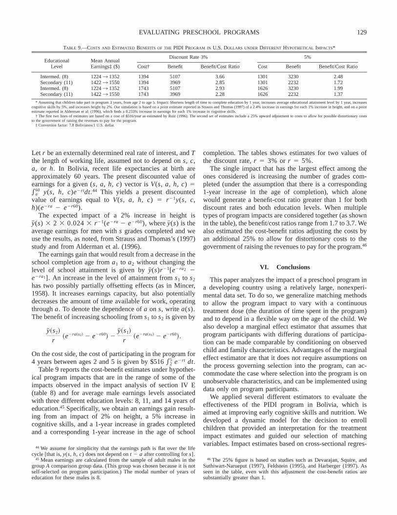
Let r be an externally determined real rate of interest, and Tthe length of working life, assumed not to depend on s, c,a, or h. In Bolivia, recent life expectancies at birth areapproximately 60 years. The present discounted value ofearnings for a given (s, a, h, c) vector is V(s, a, h, c) a
60 y(s, h, c)e�rtdt.44 This yields a present discountedvalue of earnings equal to V(s, a, h, c) r�1y(s, c,h)(e�ra � e�r60).
The expected impact of a 2% increase in height isy� (s) � 2 � 0.024 � r�1(e�ra � e�r60), where y� (s) is theaverage earnings for men with s grades completed and weuse the results, as noted, from Strauss and Thomas’s (1997)study and from Alderman et al. (1996).
The earnings gain that would result from a decrease in theschool completion age from a1 to a2 without changing thelevel of school attainment is given by y� (s)r�1[e�ra2 �e�ra1]. An increase in the level of attainment from s1 to s2
has two possibly partially offsetting effects (as in Mincer,1958). It increases earnings capacity, but also potentiallydecreases the amount of time available for work, operatingthrough a. To denote the dependence of a on s, write a(s).The benefit of increasing schooling from s1 to s2 is given by
y� �s2�
r�e�ra�s2� � e�r60� �
y� �s1�
r�e�ra�s1� � e�r60�.
On the cost side, the cost of participating in the program for4 years between ages 2 and 5 is given by $516 2
5 e�rt dt.Table 9 reports the cost-benefit estimates under hypothet-
ical program impacts that are in the range of some of theimpacts observed in the impact analysis of section IV E(table 8) and for average male earnings levels associatedwith three different education levels: 8, 11, and 14 years ofeducation.45 Specifically, we obtain an earnings gain result-ing from an impact of 2% on height, a 5% increase incognitive skills, and a 1-year increase in grades completedand a corresponding 1-year increase in the age of school
completion. The tables shows estimates for two values ofthe discount rate, r 3% or r 5%.
The single impact that has the largest effect among theones considered is increasing the number of grades com-pleted (under the assumption that there is a corresponding1-year increase in the age of completion), which alonewould generate a benefit-cost ratio greater than 1 for bothdiscount rates and both education levels. When multipletypes of program impacts are considered together (as shownin the table), the benefit/cost ratios range from 1.7 to 3.7. Wealso estimated the cost-benefit ratios adjusting the costs byan additional 25% to allow for distortionary costs to thegovernment of raising the revenues to pay for the program.46
VI. Conclusions
This paper analyzes the impact of a preschool program ina developing country using a relatively large, nonexperi-mental data set. To do so, we generalize matching methodsto allow the program impact to vary with a continuoustreatment dose (the duration of time spent in the program)and to depend in a flexible way on the age of the child. Wealso develop a marginal effect estimator that assumes thatprogram participants with differing durations of participa-tion can be made comparable by conditioning on observedchild and family characteristics. Advantages of the marginaleffect estimator are that it does not require assumptions onthe process governing selection into the program, can ac-commodate the case where selection into the program is onunobservable characteristics, and can be implemented usingdata only on program participants.
We applied several different estimators to evaluate theeffectiveness of the PIDI program in Bolivia, which isaimed at improving early cognitive skills and nutrition. Wedeveloped a dynamic model for the decision to enrollchildren that provided an interpretation for the treatmentimpact estimates and guided our selection of matchingvariables. Impact estimates based on cross-sectional regres-
44 We assume for simplicity that the earnings path is flat over the lifecycle [that is, y(s, h, c) does not depend on t � a after controlling for s].
45 Mean earnings are calculated from the sample of adult males in thegroup A comparison group data. (This group was chosen because it is notself-selected on program participation.) The modal number of years ofeducation for these males is 8.
46 The 25% figure is based on studies such as Devarajan, Squire, andSuthiwart-Narueput (1997), Feldstein (1995), and Harberger (1997). Asseen in the table, even with this adjustment the cost-benefit ratios aresubstantially greater than 1.
TABLE 9.—COSTS AND ESTIMATED BENEFITS OF THE PIDI PROGRAM IN U.S. DOLLARS UNDER DIFFERENT HYPOTHETICAL IMPACTS*
EducationalLevel
Mean AnnualEarnings‡ ($)
Discount Rate 3% 5%
Cost† Benefit Benefit/Cost Ratio Cost Benefit Benefit/Cost Ratio
Intermed. (8) 12243 1352 1394 5107 3.66 1301 3230 2.48Secondary (11) 14223 1550 1394 3969 2.85 1301 2232 1.72Intermed. (8) 12243 1352 1743 5107 2.93 1626 3230 1.99Secondary (11) 14223 1550 1743 3969 2.28 1626 2232 1.37
* Assuming that children take part in program 3 years, from age 2 to age 5. Impact: Shortens length of time to complete education by 1 year, increases average educational attainment level by 1 year, increasescognitive skills by 5%, and increases height by 2%. Our simulation is based on a point estimate reported in Strauss and Thomas (1997) of a 2.4% increase in earnings for each 1% increase in height, and on a pointestimate reported in Alderman et al. (1996), which finds a 0.233% increase in earnings for each 1% increase in cognitive skills.
† The first two lines of estimates are based on a cost of $516/year as estimated by Ruiz (1996). The second set of estimates include a 25% upward adjustment to costs to allow for possible distortionary coststo the government of raising the revenues to pay for the program.
‡ Conversion factor: 7.8 Bolivianos/1 U.S. dollar.
EVALUATING PRESCHOOL PROGRAMS 129
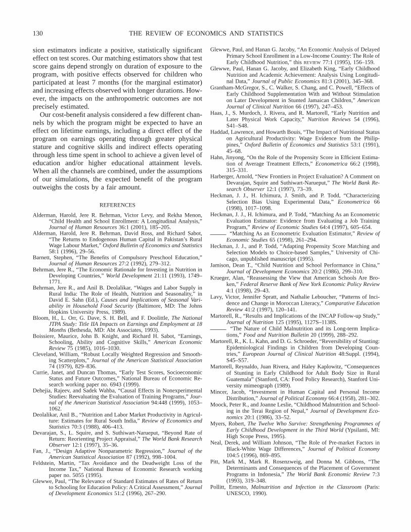
sion estimators indicate a positive, statistically significanteffect on test scores. Our matching estimators show that testscore gains depend strongly on duration of exposure to theprogram, with positive effects observed for children whoparticipated at least 7 months (for the marginal estimator)and increasing effects observed with longer durations. How-ever, the impacts on the anthropometric outcomes are notprecisely estimated.
Our cost-benefit analysis considered a few different chan-nels by which the program might be expected to have aneffect on lifetime earnings, including a direct effect of theprogram on earnings operating through greater physicalstature and cognitive skills and indirect effects operatingthrough less time spent in school to achieve a given level ofeducation and/or higher educational attainment levels.When all the channels are combined, under the assumptionsof our simulations, the expected benefit of the programoutweighs the costs by a fair amount.
REFERENCES
Alderman, Harold, Jere R. Behrman, Victor Levy, and Rekha Menon,“Child Health and School Enrollment: A Longitudinal Analysis,”Journal of Human Resources 36:1 (2001), 185–205.
Alderman, Harold, Jere R. Behrman, David Ross, and Richard Sabot,“The Returns to Endogenous Human Capital in Pakistan’s RuralWage Labour Market,” Oxford Bulletin of Economics and Statistics58:1 (1996), 29–56.
Barnett, Stephen, “The Benefits of Compulsory Preschool Education,”Journal of Human Resources 27:2 (1992), 279–312.
Behrman, Jere R., “The Economic Rationale for Investing in Nutrition inDeveloping Countries,” World Development 21:11 (1993), 1749–1771.
Behrman, Jere R., and Anil B. Deolalikar, “Wages and Labor Supply inRural India: The Role of Health, Nutrition and Seasonality,” inDavid E. Sahn (Ed.), Causes and Implications of Seasonal Vari-ability in Household Food Security (Baltimore, MD: The JohnsHopkins University Press, 1989).
Bloom, H., L. Orr, G. Dave, S. H. Bell, and F. Doolittle, The NationalJTPA Study: Title IIA Impacts on Earnings and Employment at 18Months (Bethesda, MD: Abt Associates, 1993).
Boissiere, Maurice, John B. Knight, and Richard H. Sabot, “Earnings,Schooling, Ability and Cognitive Skills,” American EconomicReview 75 (1985), 1016–1030.
Cleveland, William, “Robust Locally Weighted Regression and Smooth-ing Scatterplots,” Journal of the American Statistical Association74 (1979), 829–836.
Currie, Janet, and Duncan Thomas, “Early Test Scores, SocioeconomicStatus and Future Outcomes,” National Bureau of Economic Re-search working paper no. 6943 (1999).
Dehejia, Rajeev, and Sadek Wahba, “Causal Effects in NonexperimentalStudies: Reevaluating the Evaluation of Training Programs,” Jour-nal of the American Statistical Association 94:448 (1999), 1053–1062.
Deolalikar, Anil B., “Nutrition and Labor Market Productivity in Agricul-ture: Estimates for Rural South India,” Review of Economics andStatistics 70:3 (1988), 406–413.
Devarajan, S., L. Squire, and S. Suthiwart-Narueput, “Beyond Rate ofReturn: Reorienting Project Appraisal,” The World Bank ResearchObserver 12:1 (1997), 35–36.
Fan, J., “Design Adaptive Nonparametric Regression,” Journal of theAmerican Statistical Association 87 (1992), 998–1004.
Feldstein, Martin, “Tax Avoidance and the Deadweight Loss of theIncome Tax,” National Bureau of Economic Research workingpaper no. 5055 (1995).
Glewwe, Paul, “The Relevance of Standard Estimates of Rates of Returnto Schooling for Education Policy: A Critical Assessment,” Journalof Development Economics 51:2 (1996), 267–290.
Glewwe, Paul, and Hanan G. Jacoby, “An Economic Analysis of DelayedPrimary School Enrollment in a Low-Income Country: The Role ofEarly Childhood Nutrition,” this REVIEW 77:1 (1995), 156–159.
Glewwe, Paul, Hanan G. Jacoby, and Elizabeth King, “Early ChildhoodNutrition and Academic Achievement: Analysis Using Longitudi-nal Data,” Journal of Public Economics 81:3 (2001), 345–368.
Grantham-McGregor, S., C. Walker, S. Chang, and C. Powell, “Effects ofEarly Childhood Supplementation With and Without Stimulationon Later Development in Stunted Jamaican Children,” AmericanJournal of Clinical Nutrition 66 (1997), 247–453.
Haas, J., S. Murdoch, J. Rivera, and R. Martorell, “Early Nutrition andLater Physical Work Capacity,” Nutrition Reviews 54 (1996),S41–S48.
Haddad, Lawrence, and Howarth Bouis, “The Impact of Nutritional Statuson Agricultural Productivity: Wage Evidence from the Philip-pines,” Oxford Bulletin of Economics and Statistics 53:1 (1991),45–68.
Hahn, Jinyong, “On the Role of the Propensity Score in Efficient Estima-tion of Average Treatment Effects,” Econometrica 66:2 (1998),315–331.
Harberger, Arnold, “New Frontiers in Project Evaluation? A Comment onDevarajan, Squire and Suthiwart-Narueput,” The World Bank Re-search Observer 12:1 (1997), 73–39.
Heckman, J. J., H. Ichimura, J. Smith, and P. Todd, “CharacterizingSelection Bias Using Experimental Data,” Econometrica 66(1998), 1017–1098.
Heckman, J. J., H. Ichimura, and P. Todd, “Matching As an EconometricEvaluation Estimator: Evidence from Evaluating a Job TrainingProgram,” Review of Economic Studies 64:4 (1997), 605–654.
“Matching As an Econometric Evaluation Estimator,” Review ofEconomic Studies 65 (1998), 261–294.
Heckman, J. J., and P. Todd, “Adapting Propensity Score Matching andSelection Models to Choice-based Samples,” University of Chi-cago, unpublished manuscript (1995).
Jamison, Dean T., “Child Nutrition and School Performance in China,”Journal of Development Economics 20:2 (1986), 299–310.
Krueger, Alan, “Reassessing the View that American Schools Are Bro-ken,” Federal Reserve Bank of New York Economic Policy Review4:1 (1998), 29–43.
Lavy, Victor, Jennifer Spratt, and Nathalie Leboucher, “Patterns of Inci-dence and Change in Moroccan Literacy,” Comparative EducationReview 41:2 (1997), 120–141.
Martorell, R., “Results and Implications of the INCAP Follow-up Study,”Journal of Nutrition 125 (1995), 1127S–1138S.
“The Nature of Child Malnutrition and its Long-term Implica-tions,” Food and Nutrition Bulletin 20 (1999), 288–292.
Martorell, R., K. L. Kahn, and D. G. Schroeder, “Reversibility of Stunting:Epidemiological Findings in Children from Developing Coun-tries,” European Journal of Clinical Nutrition 48:Suppl. (1994),S45–S57.
Martorell, Reynaldo, Juan Rivera, and Haley Kaplowitz, “Consequencesof Stunting in Early Childhood for Adult Body Size in RuralGuatemala” (Stanford, CA: Food Policy Research), Stanford Uni-versity mimeograph (1989).
Mincer, Jacob, “ Investment in Human Capital and Personal IncomeDistribution,” Journal of Political Economy 66:4 (1958), 281–302.
Moock, Peter R., and Joanne Leslie, “Childhood Malnutrition and School-ing in the Terai Region of Nepal,” Journal of Development Eco-nomics 20:1 (1986), 33–52.
Myers, Robert, The Twelve Who Survive: Strengthening Programmes ofEarly Childhood Development in the Third World (Ypsilanti, MI:High Scope Press, 1995).
Neal, Derek, and William Johnson, “The Role of Pre-market Factors inBlack-White Wage Differences,” Journal of Political Economy104:5 (1996), 869–895.
Pitt, Mark M., Mark R. Rosenzweig, and Donna M. Gibbons, “TheDeterminants and Consequences of the Placement of GovernmentPrograms in Indonesia,” The World Bank Economic Review 7:3(1993), 319–348.
Pollitt, Ernesto, Malnutrition and Infection in the Classroom (Paris:UNESCO, 1990).
THE REVIEW OF ECONOMICS AND STATISTICS130
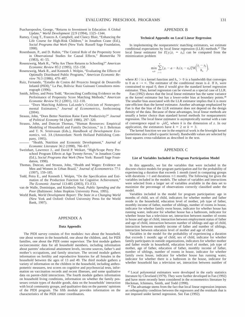
Psacharopoulos, George, “Returns to Investment in Education: A GlobalUpdate,” World Development 22:9 (1994), 1325–1344.
Ramey, Craig T., Frances A. Campbell, and Clancy Blair, “Enhancing theLife Course for High-Risk Children,” in Jonathon Crane (Ed.),Social Programs that Work (New York: Russell Sage Foundation,1998).
Rosenbaum, P., and D. Rubin, “The Central Role of the Propensity Scorein Observational Studies for Causal Effects,” Biometrika 70(1983), 41–55.
Rosenzweig, Mark R., “Why Are There Returns to Schooling?” AmericanEconomic Review 85:2 (1995), 153–158.
Rosenzweig, Mark R., and Kenneth J. Wolpin, “Evaluating the Effects ofOptimally Distributed Public Programs,” American Economic Re-view 76:3 (1986), 470–487.
Ruiz, Fernando, “Estudio de Costos del Proyecto Integral de DesarrolloInfantil (PIDI),” La Paz, Bolivia: Ruiz Guissani Consultores mim-eograph (1996).
Smith, Jeffrey, and Petra Todd, “Reconciling Conflicting Evidence on thePerformance of Propensity Score Matching Methods,” AmericanEconomic Review 91:2 (2001), 112–118.
“Does Matching Address LaLonde’s Criticism of Nonexperi-mental Estimators,” Journal of Econometrics, forthcoming(2004).
Strauss, John, “Does Better Nutrition Raise Farm Productivity?” Journalof Political Economy 94 (April 1986), 297–320.
Strauss, John, and Duncan Thomas, “Human Resources: EmpiricalModeling of Household and Family Decisions,” in J. Behrmanand T. N. Srinivasan (Eds.), Handbook of Development Eco-nomics, vol. 3A (Amsterdam: North Holland Publishing Com-pany, 1995).
“Health, Nutrition and Economic Development,” Journal ofEconomic Literature 36:2 (1998), 766–817.
Sweinhart, Lawrence J., and David P. Weikart, “High/Scope Perry Pre-school Program Effects at Age Twenty-Seven,” in Jonathon Crane(Ed.), Social Programs that Work (New York: Russell Sage Foun-dation, 1998).
Thomas, Duncan, and Strauss, John, “Health and Wages: Evidence onMen and Women in Urban Brazil,” Journal of Econometrics 77:1(1997), 159–185.
Todd, Petra E., and Kenneth I. Wolpin, “On the Specification and Esti-mation of the Production Function for Cognitive Achievement,”The Economic Journal 113:485 (2003), F3–F33.
van de Walle, Dominique, and Kimberly Nead, Public Spending and thePoor (Baltimore: Johns Hopkins University Press, 1995).
World Bank, World Development Report: The State in a Changing World(New York and Oxford: Oxford University Press for the WorldBank, 1997).
APPENDIX A
Data Appendix
The PIDI survey consists of five modules: two about the household,one about women in the household, one about the children, and, for PIDIfamilies, one about the PIDI center supervisor. The first module gatherssocioeconomic data for all household members, including informationabout parents’ educational attainment levels, income sources, father’s andmother’s occupations, and family structure. The second module gathersinformation on fertility and reproductive histories for all females in thehousehold between the ages of 13 and 49. The third module gathers avariety of information on the children in the household, including anthro-pometric measures, test scores on cognitive and psychosocial tests, infor-mation on vaccination records and recent illnesses, and some qualitativedata on parent-child interactions. The fourth module gathers informationon household living conditions, information on whether the family pos-sesses certain types of durable goods, data on the households’ interactionwith local community groups, and qualitative data on the parents’ opinionsof the PIDI program. The fifth module provides information on thecharacteristics of the PIDI center coordinators.
APPENDIX B
Technical Appendix on Local Linear Regression
In implementing the nonparametric matching estimators, we estimateconditional expectations by local linear regression (LLR) methods.47 Thelocal linear estimator for E[ yi�zi z0] can be computed from theminimization problem
mina,b
�i1
n
�yi � a � b1�zi � z0��2K�zi � z0
hn�,
where K� is a kernel function and hn � 0 is a bandwidth that convergesto 0 as n 3 �. The estimator of the conditional mean is a. If b1 wereconstrained to equal 0, then a would give the standard kernel regressionestimator. Thus, kernel regression can be viewed as a special case of LLR.
Fan (1992) shows that the local linear estimator has the same varianceas the kernel estimator but has a lower-order bias at boundary points.48
The smaller bias associated with the LLR estimator implies that it is morerate-efficient than the kernel estimator. Another advantage emphasized byFan is that the bias of the LLR estimator does not depend on the designdensity of the data. Because of these advantages, local linear methods areusually a better choice than standard kernel methods for nonparametricregression. The local linear estimator is asymptotically normal with a rateof convergence equal to nhn
k, where k is the dimension of z. In ourapplication, the estimators have k 2 or k 3.
The kernel function we use in the empirical work is the biweight kernel(sometimes also called a quartic kernel). Bandwidth values are selected byleast squares cross-validation as described in the text.
APPENDIX C
List of Variables Included in Program Participation Model
In this appendix, we list the variables that were included in thediscrete-choice models for program participation and for the probability ofexperiencing a duration that exceeds 1 month (used in comparing groupswith durations �1 and durations �1 month). The following list gives thevariables included in the models. The subset of variables and interactionswere selected from a larger set of variables available in the data set tomaximize the percentage of observations correctly classified under themodel.
Variables included in the model for program participation: age inmonths of child, sex of child, indicators for whether mother and fatherreside in the household, education level of mother, job type of father,monthly income of father, number of siblings, number of rooms in house,indicator for whether family owns house, indicator for whether house hasrunning water, indicator for whether house has a bathroom, indicator forwhether house has a television set, interaction between number of roomsin house and age of child, interaction between employment status of fatherand age of child, interaction between number of siblings and age of child,interaction between monthly income of father and number of siblings,interaction between education level of mother and age of child.
Variables in the model for the probability of experiencing a durationthat exceeds 1 month: age of child, sex of child, indicator for whetherfamily participates in outside organizations, indicators for whether motherand father reside in household, education level of mother, job type ofmother, age of father, education of father, monthly income of father,number of siblings, number of rooms in house, indicator for whetherfamily owns house, indicator for whether house has running water,indicator for whether there is a bathroom in the house, indicator forwhether household has a television set, interaction between number of
47 Local polynomial estimators were developed in the early statisticsliterature by Cleveland (1979). They were further developed in Fan (1992)and have more recently been considered in the econometrics literature byHeckman, Ichimura, Smith, and Todd (1998).
48 The advantage stems from the fact that local linear regression imposesan orthogonality condition between the regressors and the residuals that isnot imposed under kernel regression. See Fan (1992).
EVALUATING PRESCHOOL PROGRAMS 131
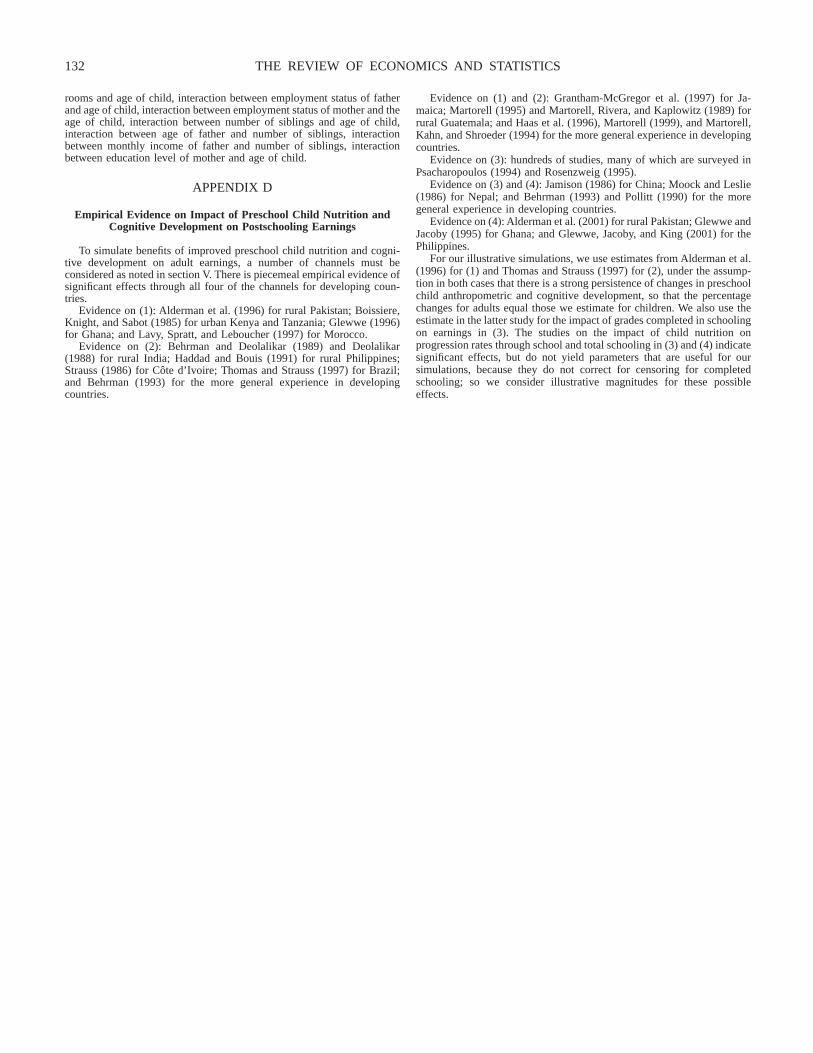
rooms and age of child, interaction between employment status of fatherand age of child, interaction between employment status of mother and theage of child, interaction between number of siblings and age of child,interaction between age of father and number of siblings, interactionbetween monthly income of father and number of siblings, interactionbetween education level of mother and age of child.
APPENDIX D
Empirical Evidence on Impact of Preschool Child Nutrition andCognitive Development on Postschooling Earnings
To simulate benefits of improved preschool child nutrition and cogni-tive development on adult earnings, a number of channels must beconsidered as noted in section V. There is piecemeal empirical evidence ofsignificant effects through all four of the channels for developing coun-tries.
Evidence on (1): Alderman et al. (1996) for rural Pakistan; Boissiere,Knight, and Sabot (1985) for urban Kenya and Tanzania; Glewwe (1996)for Ghana; and Lavy, Spratt, and Leboucher (1997) for Morocco.
Evidence on (2): Behrman and Deolalikar (1989) and Deolalikar(1988) for rural India; Haddad and Bouis (1991) for rural Philippines;Strauss (1986) for Cote d’ Ivoire; Thomas and Strauss (1997) for Brazil;and Behrman (1993) for the more general experience in developingcountries.
Evidence on (1) and (2): Grantham-McGregor et al. (1997) for Ja-maica; Martorell (1995) and Martorell, Rivera, and Kaplowitz (1989) forrural Guatemala; and Haas et al. (1996), Martorell (1999), and Martorell,Kahn, and Shroeder (1994) for the more general experience in developingcountries.
Evidence on (3): hundreds of studies, many of which are surveyed inPsacharopoulos (1994) and Rosenzweig (1995).
Evidence on (3) and (4): Jamison (1986) for China; Moock and Leslie(1986) for Nepal; and Behrman (1993) and Pollitt (1990) for the moregeneral experience in developing countries.
Evidence on (4): Alderman et al. (2001) for rural Pakistan; Glewwe andJacoby (1995) for Ghana; and Glewwe, Jacoby, and King (2001) for thePhilippines.
For our illustrative simulations, we use estimates from Alderman et al.(1996) for (1) and Thomas and Strauss (1997) for (2), under the assump-tion in both cases that there is a strong persistence of changes in preschoolchild anthropometric and cognitive development, so that the percentagechanges for adults equal those we estimate for children. We also use theestimate in the latter study for the impact of grades completed in schoolingon earnings in (3). The studies on the impact of child nutrition onprogression rates through school and total schooling in (3) and (4) indicatesignificant effects, but do not yield parameters that are useful for oursimulations, because they do not correct for censoring for completedschooling; so we consider illustrative magnitudes for these possibleeffects.
THE REVIEW OF ECONOMICS AND STATISTICS132